Full-Stack FP4: Stable LLM Pretraining with Quantized Projections, Optimizers, and Attention
July 05, 2026
Abstract
Recent NVFP4 pretraining works have primarily focused on transformer linear layers, while optimizer states, optimizer computation, and attention operators remain only partially explored in 4-bit pretraining. This gap makes stable full-stack 4-bit pretraining unattainable, because the three modules suffer from distinct numerical failure modes: linear projections face a fundamental quantization noise ceiling and dimension-scaled error amplification; AdamW second moments are non-negative, heavy-tailed, and denominator-sensitive to quantization; attention involves error-sensitive paths and requires strict forward-backward quantization consistency. We present Full-Stack FP4, the first end-to-end NVFP4 pretraining recipe that addresses all three stability bottlenecks with module-specific precision policies. For linear projections, we introduce LoRA-SVD, a light-weight structural decomposition that systematically dilutes quantization noise and escapes the error ceiling of direct quantization, reducing the linear-only loss gap from 1.40% to 0.61%. For optimizers, we design a transformation pipeline to reshape AdamW’s second moment for stable NVFP4 storage, and enable Newton–Schulz iterations of the arising Root (Muon) optimizer to run natively in NVFP4. For attention, we use a mixed-precision design that quantizes Q/K/V and backward \(dS\) while protecting sensitive paths in BF16, with consistent tensor reuse to preserve forward-backward alignment. We additionally provide lightweight analyses showing why quantization error grows rapidly with scale in direct low-bit matrix products and why the \(PV\) and \(dOV^\top\) attention paths are particularly sensitive. All components are modular with stability and additive efficiency gains. Experiments on 3B/64B-tokens pretraining show that our full-stack FP4 training maintains tight alignment with BF16 baselines, with only a 1.47% loss gap, demonstrating that stable, full-stack NVFP4 LLM pretraining is achievable. 1
Figure 1:  .
.
1 Introduction↩︎
The computational cost of LLM pretraining has driven precision down from FP32 to BF16 and FP8, with major gains in memory efficiency and throughput. Blackwell GPUs further enable native NVFP4 Tensor Core support, making 4-bit pretraining practical rather than merely theoretical. Recent work has demonstrated stable 4-bit pretraining for transformer linear layers [1]–[7], and as Muon[8] has been adopted in top models including Kimi Moonlight [9] and Deepseek-V4 [10], researchers have begun to explore low-bit Muon updates [11]. Yet the full training stack including optimizer states, optimizer computation, and attention remains uncovered.
The core question thus becomes: can we extend NVFP4 to the full pretraining stack while maintaining stability?
The challenge is that naive uniform quantization fails, because the three core modules suffer from distinct numerical failure modes: (1) Quantization Error Accumulation: Linear projections with direct NVFP4 quantization hit a fundamental quantization noise ceiling that recent works have progressively approached but cannot further reduce, with error growing linearly with hidden dimension and overwhelming optimization signals; (2) Numerical Instability: Optimizer states such as AdamW’s second moment \(v_t\) are non-negative, heavy-tailed, and denominator-sensitive, while Root’s Newton–Schulz iterations are numerically fragile in low precision; (3) Forward-Backward Path Sensitivity: Attention contains highly error-sensitive paths and requires strict forward-backward consistency to avoid divergence.
To resolve these issues, we present the first stable full-stack NVFP4 pretraining recipe that unifies quantization across linear projections, optimizer states/computation, and attention. For linear layers, we introduce LoRA-SVD, a structural decomposition that dilutes quantization noise and escapes the inherent error floor of direct 4-bit quantization; a simple error analysis explains why direct quantized matrix products become increasingly fragile as scale grows (Appendix 7). For optimizers, we design a pipeline to stabilize NVFP4 storage of AdamW’s second moment and enable NVFP4-native Newton–Schulz iterations for Root (Muon) without extra mixed-precision auxiliary operations. For attention, we propose a mixed-precision scheme that quantizes \(Q\)/\(K\)/\(V\) and \(dS\) while preserving sensitive paths in BF16, with Appendix 10 explaining why the \(PV\) and \(dOV^\top\) paths should remain in higher precision.
Our contributions are threefold: (1) We identify and formalize the three stability bottlenecks that block end-to-end FP4 pretraining, and provide lightweight analyses for the scaling of direct quantization error and the sensitivity of key attention matmuls; (2) We present, to our knowledge, the first full-stack NVFP4 recipe with module-specific policies tailored to each failure mode; (3) We validate strong alignment with BF16 baselines on 3B/64B-token pretraining, achieving only a 1.47% loss gap, while LoRA-SVD reduces the linear-only gap from 1.40% to 0.61%.
Table 1 summarizes scope. The closest full-stack pretraining works [1]–[7] present end-to-end FP4 pretraining stacks but leave optimizer states in FP32 and attention in BF16, while recent low-bit Muon work [11] focuses on optimizer quantization rather than the full pretraining stack. Ours is, to our knowledge, the first recipe that jointly compresses linear projection, optimizer(states and computation) and attention to NVFP4 within a single pretraining stack.
| Method | Prec. | Wt/Act | Opt. | Opt. | Attn | Pre- |
| State | Comp. | Quant | train | |||
| COAT [12] | FP8 | ✔ | ✔ | — | — | ✔ |
| NVFP4 [1] | FP4 | ✔ | — | — | — | ✔ |
| FP4-all-the-way [2] | FP4 | ✔ | — | — | — | ✔ |
| Quartet [3] | FP4 | ✔ | — | — | — | ✔ |
| CHON [4] | FP4 | ✔ | — | — | — | ✔ |
| 4/6 [5] | FP4 | ✔ | — | — | — | ✔ |
| TetraJet-v2 [7] | FP4 | ✔ | — | — | — | ✔ |
| Metis [13] | FP4 | ✔ | — | — | — | ✔ |
| Low-bit Muon [11] | FP4 | — | ✔ | ✔ | — | — |
| Attn-QAT [14] | FP4 | — | — | — | ✔ | \(\circ\) |
| SageAttn3 [15] | FP4 | — | — | — | ✔ | \(\circ\) |
| Ours | FP4 | ✔ | ✔ | ✔ | ✔ | ✔ |
2 Preliminaries↩︎
This section establishes the notation and background for the main computation primitives in our recipe.
NVFP4 format. NVFP4 format [1] uses E2M1 encoding (1 sign, 2 exponent, 1 mantissa) together with block-wise scaling: each block of 16x16 or 1x16 elements shares an FP8 E4M3 scale factor \(s\), and an additional FP32 global scale \(s_g\): \(\hat{x} = x_\mathrm{E2M1} \times s \times s_g\). This finer granularity yields lower quantization error [1] compared to MXFP4’s block-32 with E8M0 scale [16].
Linear projection. A transformer linear layer computes \(Y = XW^\top\) where \(W\) is the weight and \(X\) is the input activation. Training involves three GEMMs: forward, activation-gradient (\(\nabla_X = \nabla_Y W\)), and weight-gradient (\(\nabla_W = \nabla_Y^\top X\)).
AdamW optimizer. AdamW maintains two state tensors per parameter: the first-order momentum \(m_t = \beta_1 m_{t-1} + g_t\) and the second-order momentum \(v_t = \beta_2 v_{t-1} + (1{-}\beta_2)g_t^2\). The update rule requires storing both \(m_t\) and \(v_t\) at sufficient precision throughout training, occupying a substantial fraction of memory.
Root optimizer. Root [17] improves Muon [8] with soft-thresholding for first-order momentum outlier removal and robust Newton–Schulz (NS) orthogonalization iteration:\(X_{k+1} = a X_k + b X_k (X_k^\top X_k) + c X_k (X_k^\top X_k)^2\) with optimized coefficients \(a\), \(b\) and \(c\). However, Root(Muon) is not suitable for all parameters, embeddings, lm_head, norm weights, bias, and LoRA parameters still need AdamW for better performance. The dense matmuls per iteration (typically \(5\) cycles) dominate Root’s compute cost.
Attention operator. Standard multi-head attention computes \(S = QK^\top/\sqrt{d}\), \(P = \mathrm{softmax}(S)\), \(O = PV\) for each head, where \(Q, K, V \in \mathbb{R}^{N \times d}\). The most commonly used operator, FlashAttention [18], [19], implements attention in a tiled, IO-aware manner that avoids materializing the full \(N \times N\) matrix. The backward pass recomputes \(S = QK^\top/\sqrt{d}\) and \(P\), and computes \(dV = P^\top dO\), \(dP = dO \cdot V^\top\), \(dS = P \odot (dP - \mathrm{rowsum}(dO \odot O))\), \(dQ = dS \cdot K / \sqrt{d}\), \(dK = dS^\top \cdot Q / \sqrt{d}\). Overall, there are 2 matmuls in the forward pass and 5 in the backward pass, and the activation tensors (\(Q\), \(K\), \(V\)) dominate the memory and I/O cost.
Others. We use two rounding strategies. Round-to-nearest (RTN) is deterministic and maps values to the closest representable number, but introduces systematic bias. Stochastic rounding (SR) is unbiased, at the cost of added randomness. Hadamard Transformation (HT) effectively redistribute outliers at small scales such as \(16\times16\) with negligible overhead. RTN is typically used in the forward pass, while SR and HT are applied to backward gradients [1], [5], [20]. FP4-All-the-Way [2] further identified a gradient-norm threshold \(\|\mathbf{g}\| < \sqrt{3}\sigma_q\) for quantized pretraining, below which the optimization signal falls beneath quantization noise and FP4 training becomes progressively less efficient.
3 Method↩︎
3.1 Recipe Overview↩︎
| Module | Bottleneck | Precision |
|---|---|---|
| Linear proj (§3.2) | noise ceiling + dimension scaling | FP4 + BF16 LoRA-SVD |
| Optimizer (§3.3–3.4) | \(v_t\) distribution | FP4 states + FP4 matmuls |
| Attention (§3.5) | path sensitivity; fwd.-bwd. consistency | FP4 \(Q\)/\(K\)/\(V\)/\(dS\) + BF16 \(P\)/\(dO\) |
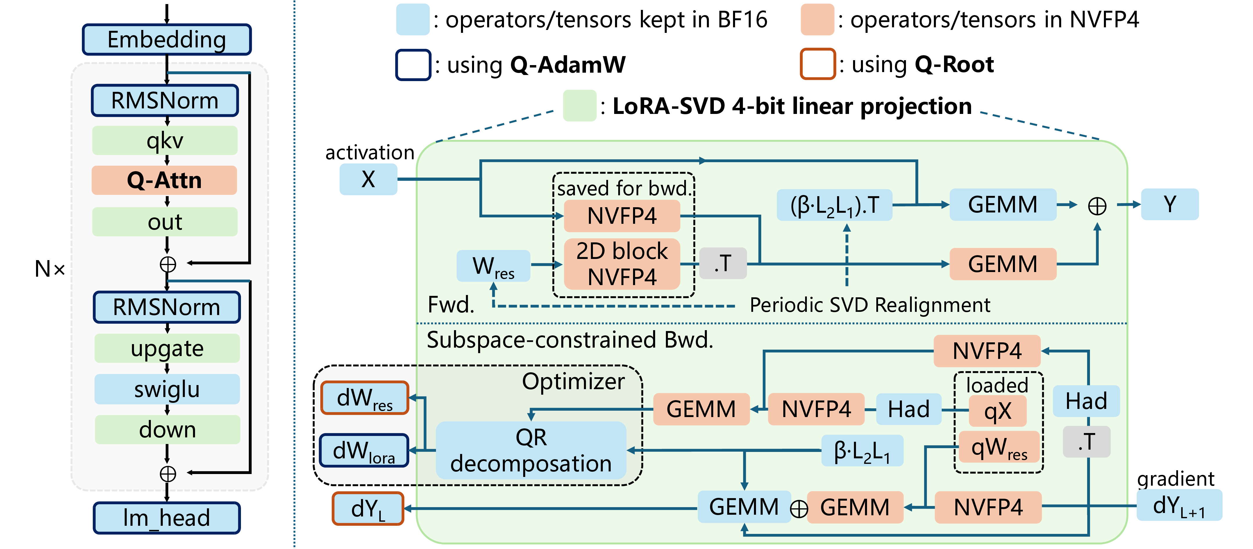
As summarized above, each component is modular and targets a distinct numerical bottleneck that limits stable full-stack FP4 pretraining. All strategies build on standard quantization primitives (RTN, SR, RHT, 4/6 scaling) while extending stable NVFP4 support to full-stack training. Figure 2 illustrates how the modules interact in a single training step.
3.2 LoRA-SVD Linear Projections↩︎
Stability Challenge: Direct NVFP4 quantization hits a fundamental noise ceiling that recent state-of-the-art scaling and rounding schemes have progressively approached but cannot further reduce. Furthermore, quantization error grows linearly with hidden dimension(Appendix 7), progressively overwhelming the optimization signal, especially in late training [2]. Purely numerical improvements can no longer push accuracy higher— a structural mechanism is needed to systematically dilute quantization noise.
To address this, we introduce LoRA-SVD, a structural decomposition that preserves a low-rank principal subspace along with the activation in BF16 while computing the residual in NVFP4. This design systematically dilutes quantization noise and bypasses the inherent error ceiling of direct 4-bit quantization. Inspired by the core idea of SVDQuant [21], such an additional branch can incur negligible overhead with proper optimization. Detailed discussions are provided in Appendix 9.
Subspace-Constrained Backward Pass. To maintain alignment with the principal subspace during training (initially guaranteed), we apply a subspace constraint using fast Cholesky-QR decomposition, the full forward and backward computations write: \[\begin{gather} Y = \underbrace{Q_\mathrm{1x16}(X)\,Q_\mathrm{16x16}(W_\mathrm{res})^\top}_{\text{NVFP4 GEMM}} + \,\beta \cdot \underbrace{(XL_1^\top)L_2^\top}_{\text{BF16}} \nonumber\\ \mathrm{d} X = Q_{\mathrm{1x16}}(\mathrm{d} Y)\,\underbrace{Q_{\mathrm{16x16}}(W_{\mathrm{res}})}_{\text{reused from fwd.}} + \beta \cdot (\mathrm{d} Y\,L_2)\,L_1 \tag{1} \\ \mathrm{d} W = Q_{\mathrm{1x16}}(\mathrm{d} Y^\top H_{16}^r) \, Q_{\mathrm{16x1}}\left({H_{16}^r}^\top Q_{\mathrm{1x16}}(X)\right) \tag{2} \\ Q_{L_2} R_{L_2} = L_2, \quad Q_{L_1} R_{L_1} = L_1^\top \tag{3} \\ \Lambda \in \mathbb{R}^{r \times r} := Q_{L_2}^\top dW Q_{L_1} \nonumber \\ dW_{\text{LoRA}} = Q_{L_2} \Lambda Q_{L_1}^\top \nonumber \\ dW_{\text{res}} = dW - dW_{\text{LoRA}} \nonumber \\ \mathrm{d} L_1 = \beta\cdot L_2^\top \mathrm{d} W_{LoRA} ,\quad \mathrm{d} L_2 = \beta \cdot \mathrm{d} W_{LoRA} L_1^\top \tag{4} \end{gather}\]
\(H_{16}^r\) denotes a \(16\times16\) random Hadamard Transformation matrix drawn fresh for each backward pass. This decomposition acts as a structural filter: components aligned with the principal subspace are routed to the BF16 LoRA branch, while quantization noise and residual components are assigned to the NVFP4 residual weight.
To avoid redundant computation during gradient accumulation, Eqs. 3 to Eqs. 4 are deferred to the optimizer, while only Eqs. 1 –2 remain inside the backward pass.Figure 3 shows that LoRA-SVD reduces relative MSE (Rel. MSE:= \(\text{MSE}(x - \hat{x}) / \text{mean}(x^2)\)) by 10% compared to direct NVFP4 quantization.
Direct LoRA gradients requires high-precision \(X\) and one more large-scale GEMM, the formulation above avoids this redundancy by using quantized activations \(Q_\mathrm{1x16}(X)\) as an approximation to improve efficiency, with full details provided in Appendix 8.
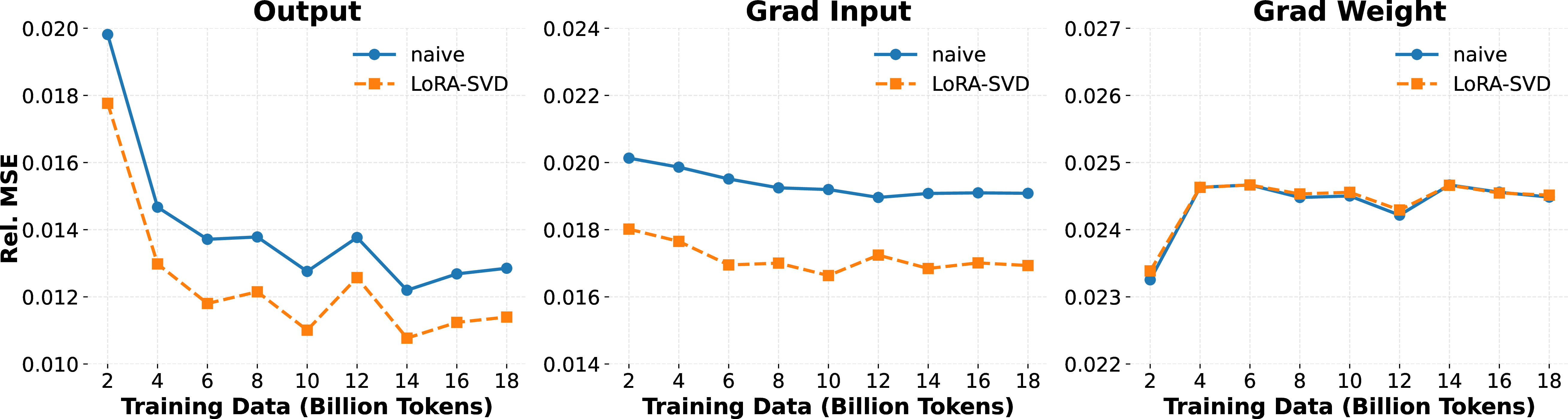
Periodic Realignment via Randomized SVD. While the subspace constraint maintains branch consistency locally during training, the total weight’s principal components inevitably evolve over time (subspace drift). To prevent this, we perform a periodic global realignment every 4k steps using fast randomized SVD [22] and reset \(W_{res},L_2, L_1\) with top-\(r\) singular components. Given that this operation is only performed every 4k steps, its computational overhead is negligible.
3.3 Quantized-State AdamW↩︎
Stability Challenge: The second moment \(v_t\) is non-negative, heavy-tailed, and acts as a denominator, thus direct NVFP4 quantization introduces large relative error and destabilizes updates, making dedicated transformations for \(v_t\) essential, consistent with the findings in [12].
While the first momentum \(m_t\) is quantized via fast Hadamard rotation, stochastic rounding (SR), and 4/6 adaptive scaling, we propose a 4-step transformed-state pipeline to reshape \(v_t\) into a distribution compatible with stable NVFP4 storage: 1) Square root: \(\tilde{v}^{(b)} = \sqrt{v^{(b)}}\) to smoothen the distribution; 2) Mean subtraction: \(\mu^{(tile)} = \text{mean}(\tilde{v}^{(tile)})\), \(\tilde{v}^{(b)} = \tilde{v}^{(b)} - \mu^{(tile)}\) to center each block. For stability and efficiency concerns, the mean is computed tile-wise; 3) Fast Hadamard Transform: \(\tilde{v}^{(b)} = \tilde{v}^{(b)}H_{16}\) to spread outlier energy with negligible \(O(16\log 16)\) overhead; 4) NVFP4 quantization: obtain \(s^{(b)}\), \(s_g\), and \(\hat{v}^{(b)}\). Reconstruction inverts the pipeline via: \(v^{(b)} \approx \left((s_g s^{(b)}\hat{v}^{(b)})H_{16} + \mu^{(b)}\right)^2\). This pipeline is critical to the viability of low-precision training, its absence would result in immediate training failure.
Figure 4 (a) shows that directly quantizing the second-order momentum leads to larger errors, while our method can significantly mitigate the compression error by around 60%. This optimization significantly improves training stability and final loss.
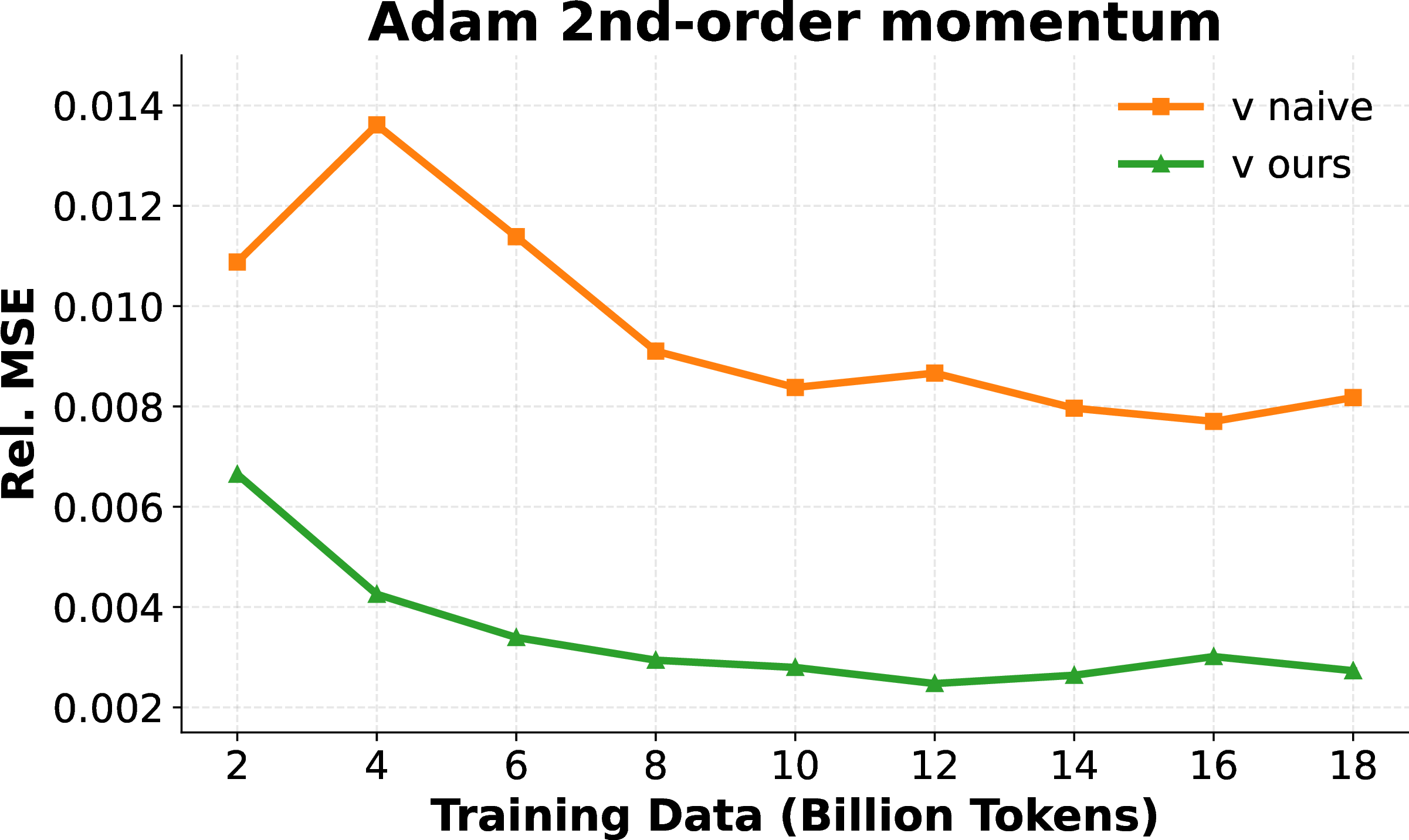

Figure 4: Optimizer quantization errors analysis. (a) Our transformed-state pipeline reduces AdamW second-moment error by \(\sim\)60%. (b) Optimized coefficients further stabilize Newton–Schulz iterations in NVFP4. Overall, the trends remain stable throughout training.. a — Quantized AdamW, b — Quantized NS iteration
3.4 NVFP4 Root Optimizer↩︎
Stability Challenge: Root’s Newton–Schulz (NS) iterations rely on repeated matmuls that are numerically sensitive to low-precision computation. This issue is particularly important in light of recent low-bit Muon results [11], which show that 4-bit Muon is feasible but require additional mixed-precision stabilization.
We enable NS iterations to run natively in NVFP4 with shape-optimized coefficients, preserving orthogonality and stability. The first order momentum or Root is the same quantization as AdamW’s. For narrow-shaped parameters, we fall back to quantized-state AdamW described in §3.3. All hyperparameters and settings follow [17].Quantized NS iteration can be described as follows:
\[\begin{gather} qX_k = Q_{\mathrm{1x16}}(XH_{16}^r),\, A_k = qX_k\,{qX_k}^\top \nonumber\\ qA_k = Q_{\mathrm{1x16}}(A_kH_{16}^r),\, qA_k^\mathrm{16x1} = Q_{\mathrm{16x1}}({H_{16}^r}^\top A_k),\, B_k = b\cdot A_k + c\cdot qA_k\,qA_k^\mathrm{16x1} \nonumber\\ qB_k = Q_{\mathrm{1x16}}(B_kH_{16}^r),\, qX_k^\mathrm{16x1} = Q_{\mathrm{16x1}}({H_{16}^r}^\top X_k),\, X_{k+1} = a\cdot X_k + qB_k\,qX_k^\mathrm{16x1} \nonumber \end{gather}\] where all NVFP4 quantizations adopt RTN and 4/6 scaling. Figure 4 (b) shows that the optimized coefficients \((a,b,c)\) for Root are critical to reducing the error of the quantized NS iteration, compared with quantization using the standard Muon coefficients [11]. Beyond their original optimization role, these shape-specialized coefficients also act as an implicit error-control mechanism under quantization: by better matching the parameter aspect ratio, they reduce the amplification of rounding noise across successive NS steps. This property is central to why our NVFP4 NS path remains fully 4-bit, without introducing extra mixed-precision auxiliary operations.
3.5 Mixed-Precision FP4 Attention↩︎
| Matmul | Pass | Operand Precision | |
|---|---|---|---|
| \(\hat{Q}\hat{K}^\top\) | Fwd | 16x16 NVFP4 \(\times\) 16x16 NVFP4 | |
| \(P\hat{V}\) | Fwd | BF16 | |
| \(\hat{Q}\hat{K}^\top\) | Bwd | 16x16 NVFP4 \(\times\) 16x16 NVFP4 | |
| \(P^\top dO\) | Bwd | BF16 | |
| \(dO \,\hat{V}^\top\) | Bwd | BF16 | |
| \(\hat{dS}\,\hat{K}\) | Bwd | 1x16 NVFP4 \(\times\) 16x16 NVFP4 | |
| \(\hat{dS}^\top\hat{Q}\) | Bwd | 1x16 NVFP4 \(\times\) 16x16 NVFP4 |
r0.55
Stability Challenge: for practical IO and memory efficiency, quantizing \(Q\)/\(K\)/\(V\) is nearly unavoidable, yet naively extending low precision to additional paths leads to severe error amplification and training instability. These critical paths are thus inherently sensitive to quantization and must remain in high precision to maintain stability. In addition, naive low-precision attention breaks forward-backward tensor consistency, as identified in [14], leading to mismatch and divergence.
We design a mixed-precision attention scheme that preserves sensitive paths in BF16 while quantizing IO‑heavy and compute‑heavy tensors, and enforces consistent quantized \(Q\)/\(K\)/\(V\) reuse between forward and backward passes, as summarized in Table 2. Under this policy, \(4\) out of \(7\) attention matmuls already involve NVFP4 operands and IO cost is largely reduced since \(Q\), \(K\), \(V\) will be loaded multiple times in both forward and backward passes.
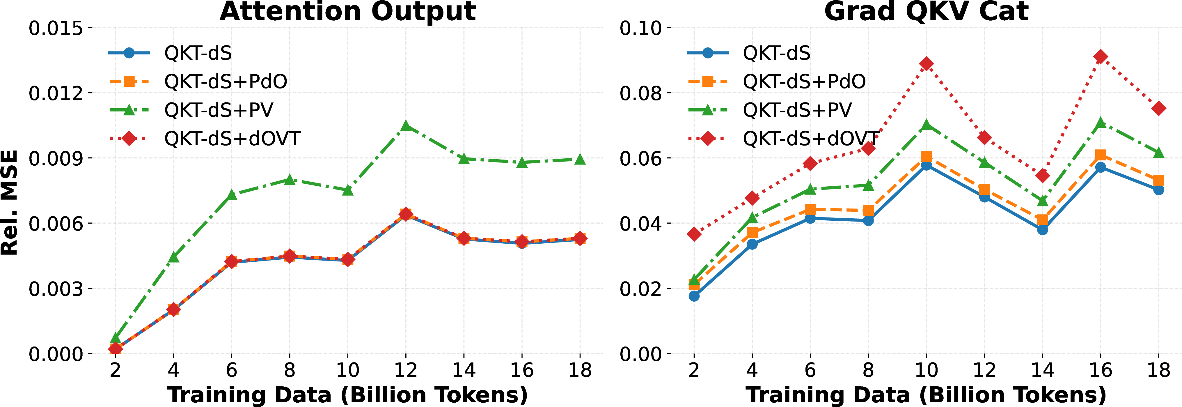
Figure 5 compares this precision split with other variants and suggest that further pushing the \(PV\) or \(dOV^\top\) paths into lower precision yields noticeably worse accuracy for only minor efficiency gains. Appendix 10 theoretically derives the numerical origins of this sensitivity, justifying our necessity to preserve these paths in BF16. \(P^\top dO\) is additionally kept in BF16 for forward-backward tensor consistency of \(P\) and stability. The fake quantization implementation follows a tiled kernel styled in FlashAttention (Appendix 11 Algorithm 8).
4 Full-Stack NVFP4 Pretraining↩︎
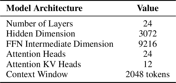
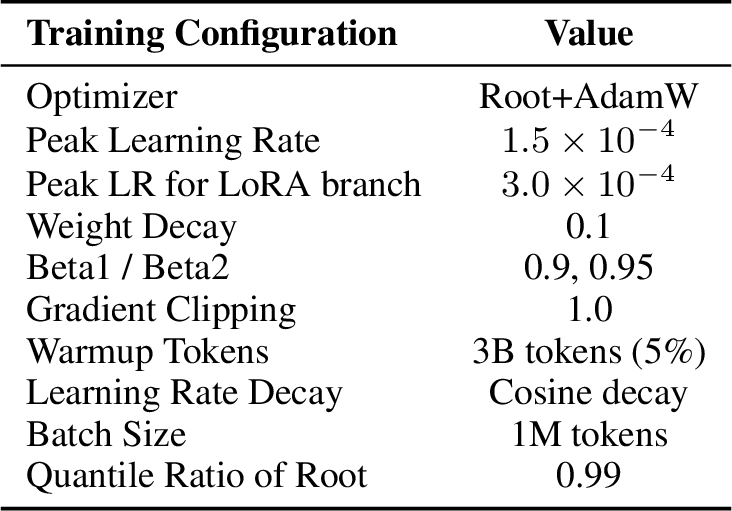
We evaluate a transformer architecture with SwiGLU and GQA at 3B scale trained on high-quality subset from Nemotron-CC v2 [23] for 64B tokens. Detailed hyperparameters are provided in Appendix 14. All experiments run on 8\(\times\)A800 80GB GPUs using fake-quantization simulation for NVFP4 training, and for quantized model, all blocks are quantized into NVFP4 with no BF16 blocks reserved like [1] does.
4.1 Main Results↩︎
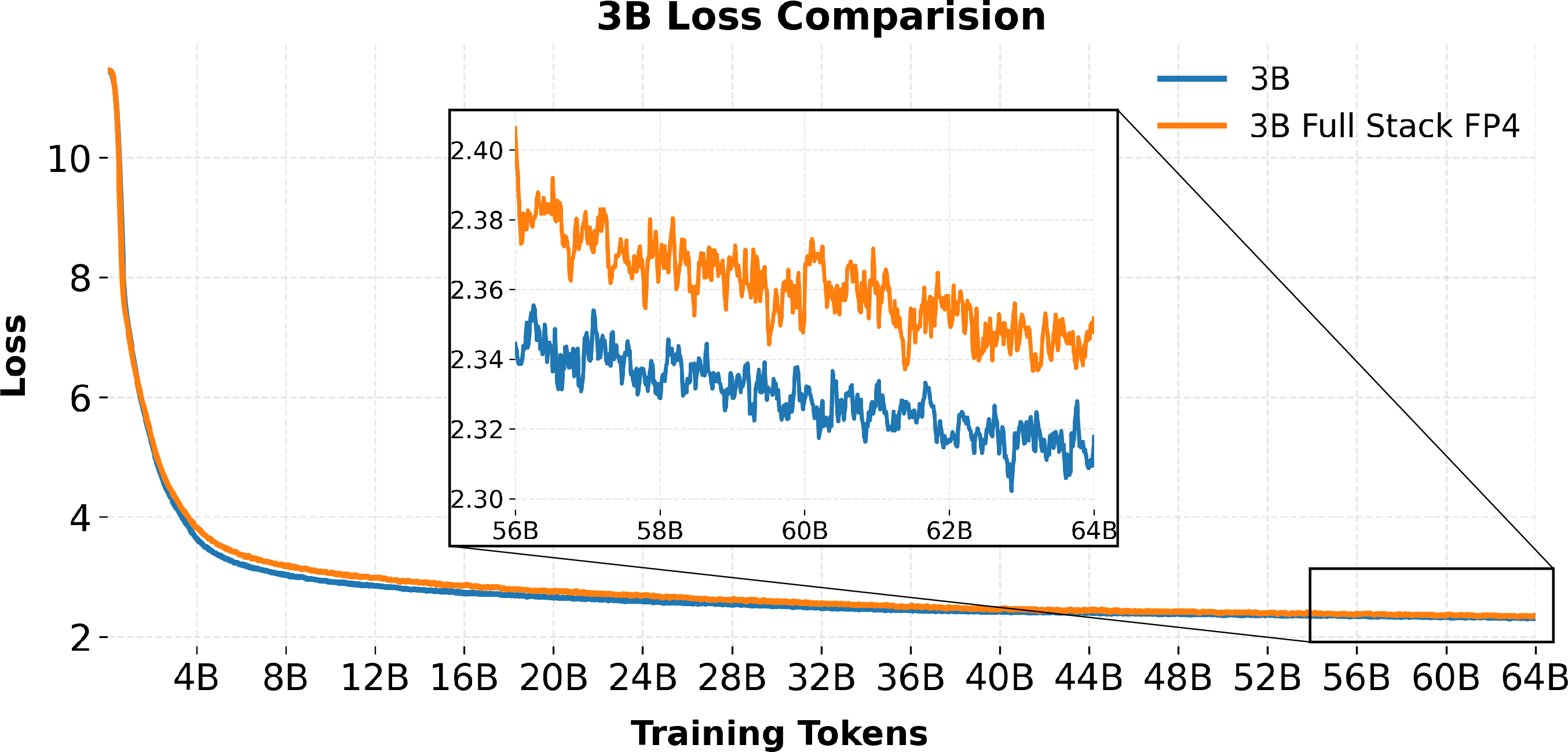
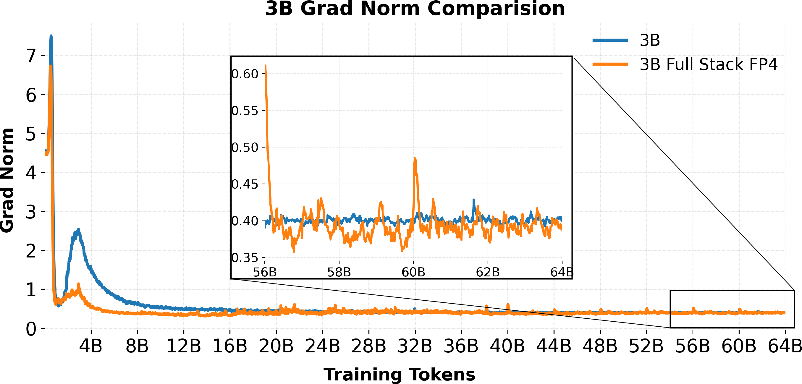
Figure 6 reports the training-loss trajectories at 3B with 64B tokens, as illustrated, our full-stack NVFP4 approach maintains tight alignment of only 1.47% loss gap with the BF16 (Root+AdamW) baseline throughout the entire pretraining process. This result demonstrates that our quantization pipeline effectively preserves optimization stability in low precision. The minimal loss gap confirms that NVFP4 quantization can be applied to full-stack Transformer pretraining without compromising core performance. The grad norm during training is reported in Appendix 12
4.2 Ablation Study↩︎
We next isolate each parts of the recipe and check for the performance in 1B model trained with 20B tokens using AdamW and Root optimizer respectively. We reimplement NVFP4+4/6 [5] using fake quantization as the state-of-the-art baseline for linear-only 4-bit pretraining. Consistent with the main experiments, all ablation studies use NVFP4 for every block with no BF16 blocks reserved.
| Configuration | Train Loss \(\downarrow\) | \(\Delta\)BF16 \(\downarrow\) |
|---|---|---|
| BF16 | 2.6415 | — |
| 4/6 | 2.6785 | +1.40% |
| 4/6 + LoRA | 2.6711 | +1.12% |
| 4/6 + LoRA-SVD | 2.6575 | +0.61% |
| 4/6 + QAdamW | 2.6674 | +0.98% |
| 4/6 + QAttn | 2.6539 | +0.47% |
| Full-stack w/o Root | 2.6563 | +0.56% |
| BF16+Root | 2.4819 | — |
| Full-stack | 2.4973 | +0.62% |
r0.55
The ablation results in Table 3 show that LoRA-SVD yields a stronger linear-only performance, narrowing the performance gap to BF16 from \(+1.40\%\) of vanilla NVFP4 4/6 [5] to \(+0.61\%\). A naive LoRA branch also brings marginal improvements, yet remains less effective than our method, as it lacks the mechanism to mitigate quantization errors. Our full-stack training recipe achieves strong alignment with the BF16 baseline, yielding a loss gap below 1% for both AdamW and Root optimizers. Appendix 13 also shows the loss landscape evolution of a toy model across training steps, verifying our full-stack design’s ability to preserve a favorable topology and avoid collapse compared to the naive NVFP4 setup.
5 Related Work↩︎
5.0.0.1 FP8/FP4 pretraining.
[24] provided an early demonstration of low-bit integer training and inference through WAGE quantization. [25] introduced FP8 training with E4M3/E5M2 per-tensor scaling, while [26] enabled stable 8-bit training for vision-language models. Extending FP8 to full pipeline, [27] and COAT [12] included optimizer states and activations, with DeepSeek-V3 [28] demonstrating 671B-scale FP8 training.For FP4/4-bit pretraining: [16] proposed the MXFP4 format and first FP4 LLM pretraining paradigm; NVFP4’s foundational methodology was established by [1], incorporating per-block quantization, stochastic rounding, and Hadamard rotation [29] for 12B-model training (10T tokens). Subsequent works improved NVFP4: [2] achieved fully quantized (weights+activations+gradients) 7B-model training (200B tokens); Quartet [3] derived FP4 scaling laws and optimized Blackwell kernels; 4/6 [5] added MSE-optimal adaptive block scaling; TetraJet [6] and its successor TetraJet-v2 [7] addressed weight oscillation via EMA quantization, outlier clipping, and adaptive updates; CHON [4] analyzed outlier dynamics and proposed hot-channel compensation.Complementary efforts include [30] (FP4 QAT with differentiable gradient estimation), [20] (MXFP4 gradient quantization with randomized Hadamard rotation), and Metis [13] (dynamic spectral decomposition for anisotropic distributions). Notably, all these works focus on linear-layer quantization—–none compress optimizer states to FP4 or quantize the attention operator for pretraining.
5.0.0.2 Low-bit optimizers.
[31] introduce INT8 block-wise Adam states. COAT [12] extends to FP8 with dynamic range expansion. [32] push Adam states to 4-bit using rank-1 normalization. [33] study INT8 quantization of Muon momentum. [11] study 4-bit Muon with subspace-preserving and grid-quantized mixed-precision stabilization.
5.0.0.3 Low-bit attention.
The SageAttention series [15], [34], [35] progressively pushes attention precision from INT8 to FP4 for inference, however, SageAttention3’s frontier training kernel is limited to INT8. Attn-QAT [14] targets FP4 attention for inference via quantization-aware training, identifying backward-pass recomputation mismatch as the key stability challenge. All these approaches build on the IO-aware tiling paradigm of FlashAttention [18], [19]; [36] study hybrid FP8 (HFP8) formatattention in earlier work. Our work differs in targeting pretraining from scratch with a mixed-precision design that reduces memory and computation cost in pretraining stage.
6 Conclusion and Limitations↩︎
We present Full-Stack FP4, the first stable end-to-end NVFP4 pretraining recipe that covers linear projections, optimizer states & computation, and attention operators. A key insight of this work is that full-stack 4-bit stability requires treating each module’s unique failure mode separately: LoRA-SVD systematically dilutes quantization noise and breaks through the error ceiling of direct 4-bit linear layers; a transformed-state pipeline stabilizes quantization of optimizer states and Root’s Newton–Schulz iterations are made NVFP4-native; mixed-precision attention protects sensitive paths and enforces forward-backward consistency. Two lightweight analyses further support these design choices by explaining the rapid growth of direct quantization error with scale and the sensitivity of the \(PV\) and \(dOV^\top\) attention paths. Our recipe is modular and additive: LoRA-SVD reduces the linear-only loss gap from 1.40% to 0.61%, and the full-stack system maintains nearly identical convergence with only a 1.47% loss gap to BF16 baselines at 3B/64B tokens with all blocks in NVFP4, proving that practical, stable full-stack FP4 LLM pretraining is feasible.
Outlook on the Ideal 4-Bit Full-Stack Pretraining Paradigm. We envision full-stack 4-bit pretraining’s core value as boosting efficiency and cutting resource overhead during LLM pretraining. However, the inherent quantization errors and noises makes full 4-bit pretraining naturally unsustainable for the entire lifecycle. LoRA-SVD provides a natural solution: it stabilizes low-precision training and supports flexible transition paths—–either merging back to full-precision weights or acting as adapters for cpt or fine-tuning. A practical workflow could use dynamic precision switching: full 4-bit early training, incremental high-precision restoration in later stages (first gradients, then forward propagation if needed), and final post-training quantization for deployment. This workflow unifies low-cost training, stable convergence, and efficient deployment for large-scale LLM development, and thus might be the reasonable solution for industrial usage.
Limitations. Given hardware resource constraints, our evaluation focuses on 3B-scale pretraining with a 64B-token budget (below the Chinchilla scaling law). While the performance alignment with BF16 stabilizes early in training, the generalization of the proposed approach to longer training horizons and larger model scales remains an important direction for further exploration. Additionally, the SVD and QR operations leveraged in our framework could benefit from specialized CUDA kernel optimizations to unlock greater efficiency. Future work may also extend to optimized end-to-end CUDA implementations of the full-stack pipeline, alongside comprehensive speed benchmarks on advanced hardware platforms such as Blackwell GPUs.
7 Appendix: Quantization Noise in Matrix Products↩︎
We derive the variance of the output error for a quantized inner product, accounting for the non-uniform NVFP4 quantization grid.
7.0.0.1 Setup.
Let \(Y = \sum_{i=1}^N x_i w_i\) be a true inner product, and \(\hat{Y} = \sum_{i=1}^N \hat{x}_i \hat{w}_i\) its quantized version, where \(\hat{x}_i = x_i + \delta_{x,i}\), \(\hat{w}_i = w_i + \delta_{w,i}\). Assume (all conditional on fixed block scales): (A1) \(\delta_{x,i}\) and \(\delta_{w,j}\) are mutually independent for all \(i,j\); (A2) \(\delta_{x,i}\) is independent of \(w_j\) for all \(j\), and vice versa; (A3) \(\mathbb{E}[\delta_{x,i}] = \mathbb{E}[\delta_{w,i}] = 0\) (stochastic rounding).
Note: Assumptions (A1) and (A3) hold exactly for SR with independent rounding draws. For shared block scales, errors within the same block are weakly coupled through the common scale; we treat Eq. 5 as an approximation in this regime. For RTN, (A3) fails (RTN has signal-dependent deterministic error), and (A1) fails across time steps; the variance formula below applies only to the SR case.
7.0.0.2 Error decomposition.
\[\begin{align} \delta Y &= \hat{Y} - Y = \sum_{i=1}^N (x_i \delta_{w,i} + w_i \delta_{x,i} + \delta_{x,i}\delta_{w,i}) \nonumber \end{align}\] Under (A3), \(\mathbb{E}[\delta Y] = 0\). For the variance, cross-terms between different indices \(i \neq j\) vanish by (A1): \[\begin{align} \mathrm{Var}(\delta Y) &= \sum_{i=1}^N \mathrm{Var}(x_i \delta_{w,i} + w_i \delta_{x,i} + \delta_{x,i}\delta_{w,i}) \nonumber \end{align}\] Expanding each term (using independence between \(\delta_x\) and \(\delta_w\)): \[\begin{align} \mathrm{Var}(\delta Y) &= \sum_{i=1}^N \bigl(x_i^2 \sigma_{w,i}^2 + w_i^2 \sigma_{x,i}^2 + \sigma_{x,i}^2 \sigma_{w,i}^2\bigr), \label{eq:app-var} \end{align}\tag{5}\] where \(\sigma_{x,i}^2 = \mathrm{Var}(\delta_{x,i})\) and \(\sigma_{w,i}^2 = \mathrm{Var}(\delta_{w,i})\).
7.0.0.3 Per-element quantization variance.
For NVFP4 E2M1 with non-uniform steps \(\Delta \in \{0.5, 0.5, 0.5, 0.5, 1.0, 1.0, 2.0\}\) across the intervals \([0, 2]\), \([2, 4]\), \([4, 6]\):
NVFP4 quantization bins. After dividing by the block scale, values are quantized to the E2M1 grid. The non-negative interior bins are: \([0, 0.25)\), \([0.25, 0.75)\), \([0.75, 1.25)\), \([1.25, 1.75)\), \([1.75, 2.5)\), \([2.5, 3.5)\), \([3.5, 5.0), [5.0, \infty)\), with step sizes \(\Delta_k \in \{0.5, 0.5, 0.5, 0.5, 1.0, 1.0, 2.0\}\). Negative values are handled symmetrically. The \(\Delta^2/12\) (RTN) and \(\Delta^2/6\) (SR) formulas below apply only to interior bins; the saturation cell requires separate treatment (in practice, per-block scaling keeps most values within the representable range, so saturation affects a small fraction of elements).
Round-to-nearest (RTN): For a fixed input \(u\) in bin \([c_k, c_{k+1}]\), RTN produces a deterministic error \(\delta = Q_\mathrm{RTN}(u) - u\) with \(|\delta| \leq \Delta_k/2\). The mean squared error averaged over inputs uniformly distributed within the bin is: \[\mathrm{MSE}_{\mathrm{RTN},k} = \frac{1}{\Delta_k}\int_0^{\Delta_k} \min(d, \Delta_k - d)^2\,dd = \frac{\Delta_k^2}{12} \nonumber\] We emphasize that this is an input-averaged MSE, not a “variance” from rounding randomness (RTN has no randomness). For non-uniform input distributions (e.g., Gaussian), the MSE may differ.
Stochastic rounding (SR): For \(u \in [c_k, c_{k+1}]\) with \(d = u - c_k\), SR rounds to \(c_{k+1}\) with probability \(d/\Delta_k\) and to \(c_k\) otherwise. The conditional variance (which is genuine rounding randomness) is: \[\sigma_{\mathrm{SR},k}^2(u) = d(\Delta_k - d) \leq \frac{\Delta_k^2}{4} \nonumber\] Averaging over \(u\) uniformly distributed in the bin: \[\mathbb{E}_u[\sigma_{\mathrm{SR}}^2] = \frac{1}{\Delta_k} \int_0^{\Delta_k} d(\Delta_k - d)\,dd = \frac{\Delta_k^2}{6} \nonumber\] For non-uniform input distributions, the effective average \(\mathbb{E}[d(\Delta_k - d)]\) depends on how mass is distributed within the bin; it may be above or below \(\Delta_k^2/6\). SR satisfies (A1)–(A3) approximately (exactly for independent rounding draws with fixed block scales).
7.0.0.4 Scaling with hidden dimension.
If inputs are drawn such that \(\mathbb{E}[x_i^2] = \bar{x}^2\) for all \(i\), and quantization variance is approximately homogeneous \(\sigma_{x,i}^2 \approx \sigma_x^2\), then: \[\mathrm{Var}(\delta Y) \approx N\bigl(\bar{x}^2 \sigma_w^2 + \bar{w}^2 \sigma_x^2 + \sigma_x^2 \sigma_w^2\bigr) = \Theta(N) \nonumber\] confirming linear growth with hidden dimension. For a full matrix product \(\hat{Y} = \hat{X}\hat{W}^\top\) where \(X \in \mathbb{R}^{B \times N}\) and \(W \in \mathbb{R}^{M \times N}\), each output element \(\hat{Y}_{ij}\) has variance \(\Theta(N)\), and the total Frobenius error \(\|\hat{Y} - Y\|_F^2\) scales as \(\Theta(BMN)\).
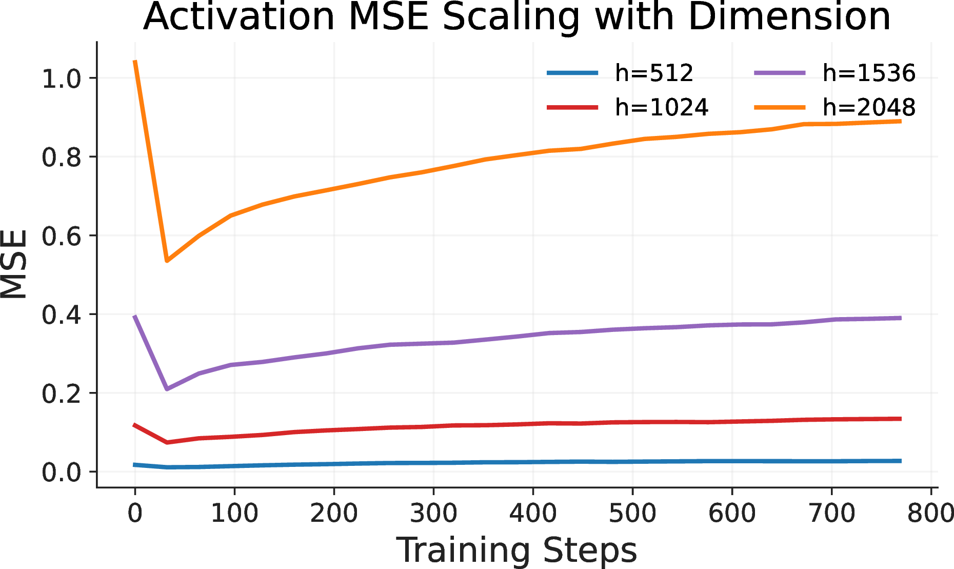
In fact, due to layer-wise error accumulation, the MSE error introduced by quantization grows faster than linearly with increasing dimension size. Figure 7 plots the final-block output activation quantization MSE from a small-scale toy training setup with 6 network layers, where the hidden dimension expands from 512 to 2048 (corresponding to a parameter growth from 50M to 400M). As observed, quantization MSE rises markedly as the dimension increases. Moreover, such error is well suppressed in the early training stage and gradually increases as training proceeds.
8 Appendix: Full Derivation of LoRA-SVD↩︎
The aligned forward and naive backward computations are: \[\begin{gather} Y = \underbrace{Q_\mathrm{1x16}(X)\,Q_\mathrm{16x16}(W_\mathrm{res})^\top}_{\text{NVFP4 GEMM}} + \,\beta \cdot \underbrace{(XL_1^\top)L_2^\top}_{\text{BF16}} \nonumber\\ \mathrm{d} X = Q_{\mathrm{1x16}}(\mathrm{d} Y)\,\underbrace{Q_{\mathrm{16x16}}(W_{\mathrm{res}})}_{\text{reused from fwd.}} + \beta \cdot (\mathrm{d} Y\,L_2)\,L_1 \nonumber \\ \mathrm{d} W = Q_{\mathrm{1x16}}(\mathrm{d} Y^\top H_{16}^r) \, Q_{\mathrm{16x1}}\left({H_{16}^r}^\top Q_{\mathrm{1x16}}(X)\right) \nonumber \\ \mathrm{d} W_{\mathrm{res}} = \mathrm{d} W \nonumber \\ \mathrm{d} L_1 = \beta\cdot L_2^\top (\mathrm{d} Y^\top \,X) \nonumber \\ \mathrm{d} L_2 = \beta \cdot (\mathrm{d} Y^\top \,X) L_1^\top \nonumber \end{gather}\]
The forward pass uses RTN and the backward pass adopts SR, while both use 4/6 scaling. \(H_{16}^r\) denotes a \(16\times16\) random Hadamard Transformation matrix drawn fresh for each backward pass. Notably, computing \(dL_1\) and \(dL_2\) separately entails the same dominant large-scale GEMM as \(dW_{\mathrm{res}}\). To avoid duplicating this cost, we reuse the already-formed \(\mathrm{d}W\) and rewrite: \[\mathrm{d} L_1 = \beta\cdot L_2^\top \mathrm{d} W ,\quad \mathrm{d} L_2 = \beta \cdot \mathrm{d} W L_1^\top \nonumber\] This change is motivated by efficiency since these gradients require full-precision X to align with the forward pass mathematically, but eventually it works well.
To ensure the LoRA branch consistently captures the principal components of the SVD during training (initially guaranteed), we thus introduce a subspace constraint based on fast Cholesky-QR decomposition: \[Q_{L_2} R_{L_2} = L_2, \qquad Q_{L_1} R_{L_1} = L_1^\top, \nonumber\] where Cholesky-QR computes \(R = \mathrm{chol}(A^\top A)^\top \in \mathbb{R}^{r \times r}\) and \(Q = A R^{-1} \in \mathbb{R}^{d \times r}\), which is faster than Householder QR for tall-thin matrices (\(r \ll d,d_o\)). Then: \[\begin{gather} \Lambda = Q_{L_2}^\top\,dW\,Q_{L_1},\quad \Lambda \in \mathbb{R}^{r \times r} \nonumber\\ \mathrm{d}W_{LoRA} = Q_{L_2}\,\Lambda\,Q_{L_1}^\top \nonumber\\ \mathrm{d}W_{res} = \mathrm{d}W - \mathrm{d}W_{LoRA} \nonumber\\ \mathrm{d} L_1 = \beta\cdot L_2^\top \mathrm{d} W_{LoRA} ,\qquad \mathrm{d} L_2 = \beta \cdot \mathrm{d} W_{LoRA} L_1^\top, \nonumber \end{gather}\]
9 Appendix: Kernel Fusion Discussion of LoRA-SVD↩︎
We focus on the \(Y\) and \(\mathrm{d}X\) computation of the LoRA-SVD branch, as both involve heavy I/O of high-precision large-scale \(X\), \(\mathrm{d}Y\), and their corresponding output tensors. In this section, we discuss and analyze the possibility of integrating its computation and memory access efficiently into existing quantization kernels.
In low-precision training pipelines, the quantization kernel for activation \(X\) can be fused with preceding operations such as layer normalization or SwiGLU. Even when full end-to-end fusion is not enabled, the quantization of \(X\) still serves as a standalone dedicated kernel for the output projection after self-attention. Similarly, a separate quantization kernel is always required for \(\mathrm{d}Y\).
The tiling layout of these quantization kernels can adopt row-wise partitioning inherited from normalization modules, or block-wise partitioning as commonly used in SwiGLU and standalone quantization kernels.
A key insight from SVDQuant [21]—originally designed for post-training quantization and inference—is that naively deploying an independent low-rank branch incurs substantial latency overhead in low-bit inference, with up to 57% slowdown caused by redundant movement of 16-bit activations and repeated DRAM access. To mitigate this issue, SVDQuant develops the Nunchaku inference engine to fuse low-rank branch computations with quantization and 4-bit compute kernels. This design eliminates intermediate DRAM read/write traffic and reduces redundant kernel launches.
Specifically, SVDQuant fuses down-projection (\(L_1\)) with quantization by reusing the same input tensor, and fuses up-projection (\(L_2\)) with 4-bit GEMM by sharing the same output tensor. Such kernel fusion halves memory traffic and constrains the overhead of the low-rank branch to merely 5–10% in latency. Since our LoRA-SVD branch also adopts a small-rank design and shares a highly similar computation scenario, the kernel fusion paradigm can be directly reused for both \(Y\) and \(\mathrm{d}X\) calculation. With appropriate hardware-aware tiling and kernel fusion, the additional overhead introduced by our LoRA-SVD branch can be made nearly negligible.
10 Theoretical Analysis of Quantization Sensitivity in Attention↩︎
In this section, we theoretically formalize why the forward matmul \(PV\) and the backward matmul \(dO V^\top\) are inherently sensitive to ultra-low precision, necessitating their computation in BF16 as empirically demonstrated in Section 3.5. Our analysis models the interaction between the non-linear truncation of NVFP4’s 1x16 fine-grained scaling and the highly skewed numerical characteristics of the Softmax distribution.
10.1 Sensitivity of \(PV\): Block-wise Simplex Violation↩︎
In the forward pass, the exact attention matrix \(P \in \mathbb{R}^{N \times N}\) represents a convex combination satisfying the probability simplex constraint: \(\sum_{j} P_{i,j} = 1\) and \(P_{i,j} \ge 0\). The Softmax operation dictates that \(P\) is highly skewed, dominated by a few probability peaks alongside a dense, heavy tail of near-zero values.
When \(P\) is quantized to \(\hat{P}\) using NVFP4 with a 1x16 block size, the scale factor for each block \(b\) is dictated by its local maximum: \(s_b = \max_{j \in \text{block}_b} |P_{i,j}| / 6.0\). Within a 16-element block containing a probability peak, \(s_b\) is exceedingly large. Consequently, the sub-maximum probabilities fall below the representable FP4 dynamic range and are irreversibly truncated to zero.
This block-wise truncation induces a critical Simplex Violation. The row sums of the quantized matrix strictly deviate from unity (\(\sum_j \hat{P}_{i,j} \neq 1\)). Since the convex combination property is mathematically broken, the quantized output \(\hat{O} = \hat{P}V\) inherently suffers a structured, compounding norm shift proportional to \(|1 - \sum_j \hat{P}_{i,j}| \lVert V \rVert\). This systematic bias propagates exponentially across deep transformer layers, inevitably degrading forward pass stability.
10.2 Sensitivity of \(dO V^\top\): Distribution Misalignment and Spurious Gradients↩︎
In memory-efficient, FlashAttention-style backward kernels, the exact gradient w.r.t. the pre-softmax scores is formulated as: \[dS_{i,j} = P_{i,j} \left( dP_{i,j} - D_i \right) \nonumber\] where \(dP_{i,j} = \langle dO_i, V_j \rangle\). The baseline \(D_i = \sum_k P_{i,k} dP_{i,k}\) is computed natively in high precision via the identity \(D_i \equiv \langle O_i, dO_i \rangle\).
When the \(dO V^\top\) matmul is quantized to NVFP4, it introduces a truncation noise \(\Delta dP_{i,j}\). Since the baseline \(D_i\) remains exact and decoupled from this GEMM, the perturbed gradient inherently isolates this noise, scaled by the attention probability: \[\label{eq:spurious95grad} \widehat{dS}_{i,j} = P_{i,j} \left( dP_{i,j} + \Delta dP_{i,j} - D_i \right) = dS_{i,j} + P_{i,j} \Delta dP_{i,j}\tag{6}\]
The sensitivity of this path arises from the Distribution Misalignment between the Softmax probabilities \(P\) and the gradient magnitudes \(dP\). In the 1x16 per-group quantization of NVFP4, the scale factor is determined by the absolute maximum gradient within the block. While this maximum value is preserved with high fidelity (\(\Delta dP_{\text{max}} \approx 0\)), the sub-maximum gradients within the same block suffer from severe quantization noise (\(\Delta dP_{\text{sub}} \gg 0\)).
Crucially, the magnitude of a token’s gradient \(dP_{i,j}\) does not strictly correlate with its probability mass \(P_{i,j}\). Consider a token at index \(c\) that represents a significant probability peak in the Softmax distribution (\(P_{i,c} \gg 0\)). If its corresponding gradient \(dP_{i,c}\) happens to be a sub-maximum within its hardware quantization block, it incurs massive truncation noise \(\Delta dP_{i,c}\).
According to Equation 6 , this noise is directly scaled by the substantial probability mass \(P_{i,c}\). For a token at a probability peak, its exact mathematical gradient \(dS_{i,c}\) is inherently near-zero (since \(dP_{i,c} \approx D_i\)). Consequently, the injected truncation noise fundamentally dominates the true signal: \[\widehat{dS}_{i,c} \approx dS_{i,c} + P_{i,c} \cdot \Delta dP_{i,c} \nonumber\] where the magnitude of the noise may completely overshadows the signal (\(|P_{i,c} \cdot \Delta dP_{i,c}| \gg |dS_{i,c}|\)).
This dynamic causes a catastrophic degradation in the Signal-to-Noise Ratio (SNR). For tokens in the dense tail (\(P \to 0\)), the noise term \(P \cdot \Delta dP\) is safely attenuated. However, for primary or secondary probability peaks, the unmitigated truncation noise completely replaces the vanishing true gradient. This spurious gradient artificially corrupts the updates for the most critical queries and keys, destroying the attention formulation in subsequent iterations. Retaining \(dO V^\top\) in BF16 bypasses this misalignment-induced SNR degradation, ensuring stable optimization.
11 Appendix: Mixed-Precision Attention Algorithm↩︎
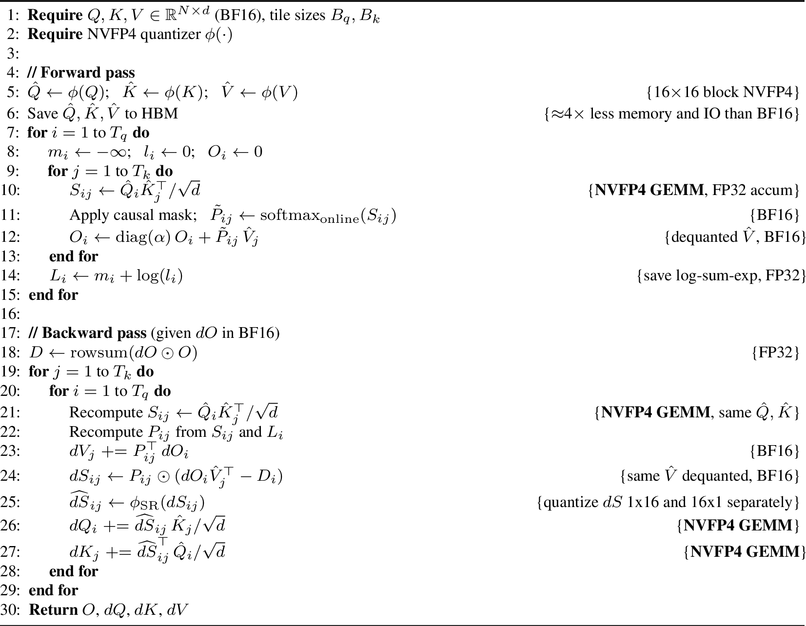
Algorithm 8 presents the FlashAttention-style forward and backward pass with NVFP4 quantization of \(Q\), \(K\), \(V\) and \(dS\).
11.0.0.1 Distinction from Attn-QAT.
Attn-QAT [14] targets inference efficiency and quantizes all attention tensors in the forward pass (including \(P\)) using fake-quantization with QAT fine-tuning, but no matmuls in backward. Our design targets on pretraining efficiency and stability and quantizes \(Q\), \(K\), \(V\) in forward and \(dS\) in backward, keeping \(P\) and \(dO\) in BF16.
12 Appendix: Gradient Norm in 3B Pretraining↩︎
Our full-stack FP4 training yields gradient norms that are both comparable and stable when compared with full-precision training, as visualized in Figure 9.
13 Appendix: Loss Landscape of a Toy Model Pretraining↩︎
To further validate the stability of our full-stack framework, we visualize the loss landscape evolution during the small-scale pretraining of a toy model (150M parameters, 6 layers, hidden dimension = 1024). We present loss landscapes at four key training steps (32, 384, 512, and 672) in Figure 10, where the four subfigures are arranged vertically in chronological order of training steps.
Each subfigure follows a consistent three-column layout for direct comparison: - Column 1: Loss landscape of the high-precision baseline; - Column 2: Loss landscape of our proposed full-stack framework; - Column 3: Loss landscape of a naive NVFP4 baseline, which adopts direct NVFP4 precision for all linear layers, all attention matrix multiplications, and AdamW optimizer.
Notably, the naive NVFP4 baseline in Column 3 suffers from training collapse after a certain step. For the final step (672 steps), the corresponding subplot in Column 3 is left blank and marked as derived to indicate the invalid state.
As observed from the vertical sequence of landscapes: - The high-precision baseline maintains a smooth optimization path throughout training, while our full-stack framework exhibits a relatively steeper yet equally smooth loss landscape—this reflects efficient gradient propagation and enables stable convergence; - In contrast, the naive NVFP4 baseline gradually develops a rugged loss landscape with an increasing number of local minima. This structural degradation exacerbates optimization difficulties and ultimately leads to training collapse at later steps.
These visualizations quantitatively confirm that our full-stack design not only mitigates quantization errors but also preserves a favorable loss landscape topology, which is critical for stable low-precision pretraining. With the steeper landscape observation, we suggest a smaller learning rate might be suitable for NVFP4 pretraining.
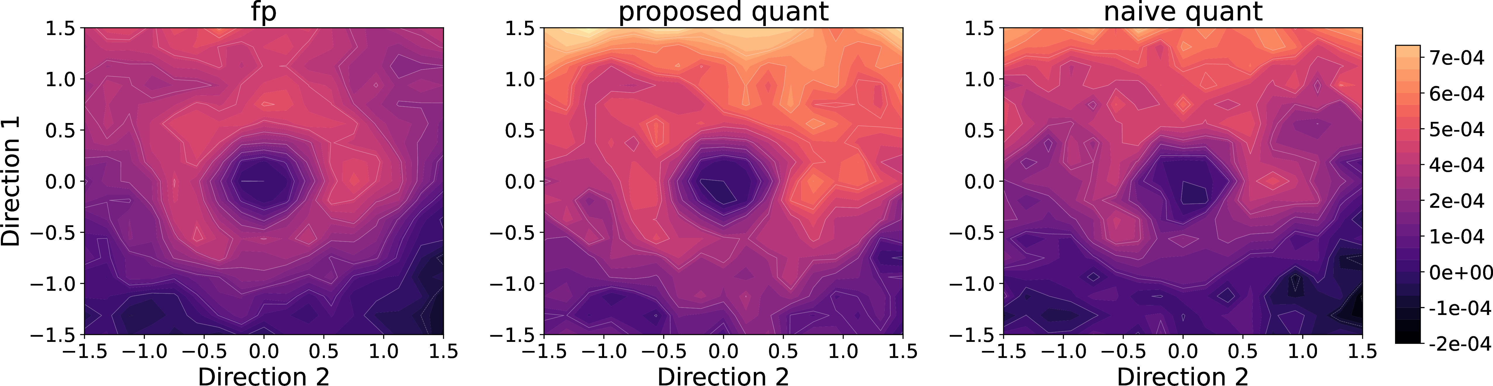
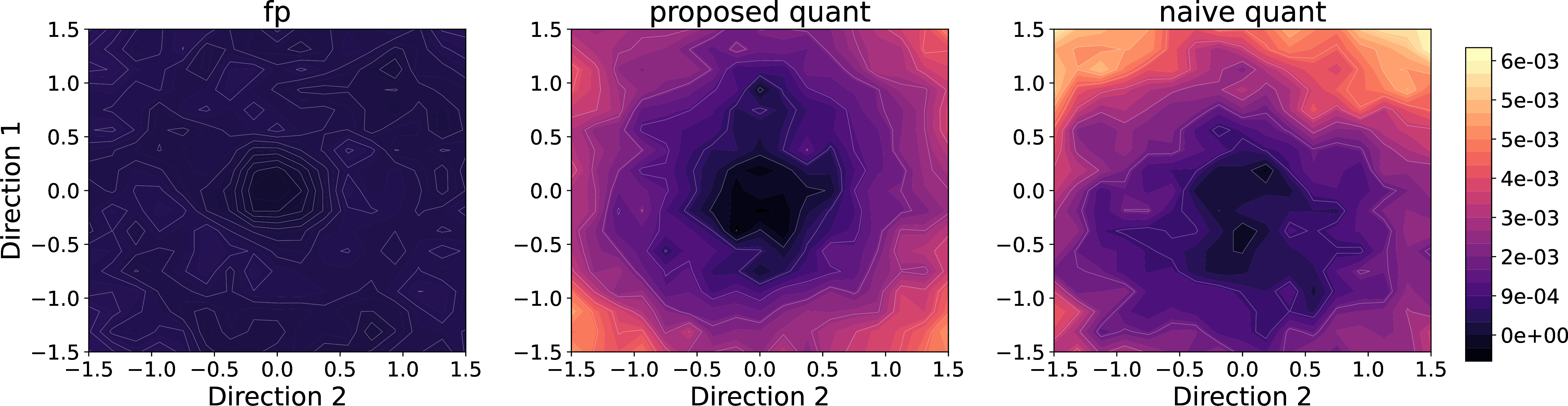
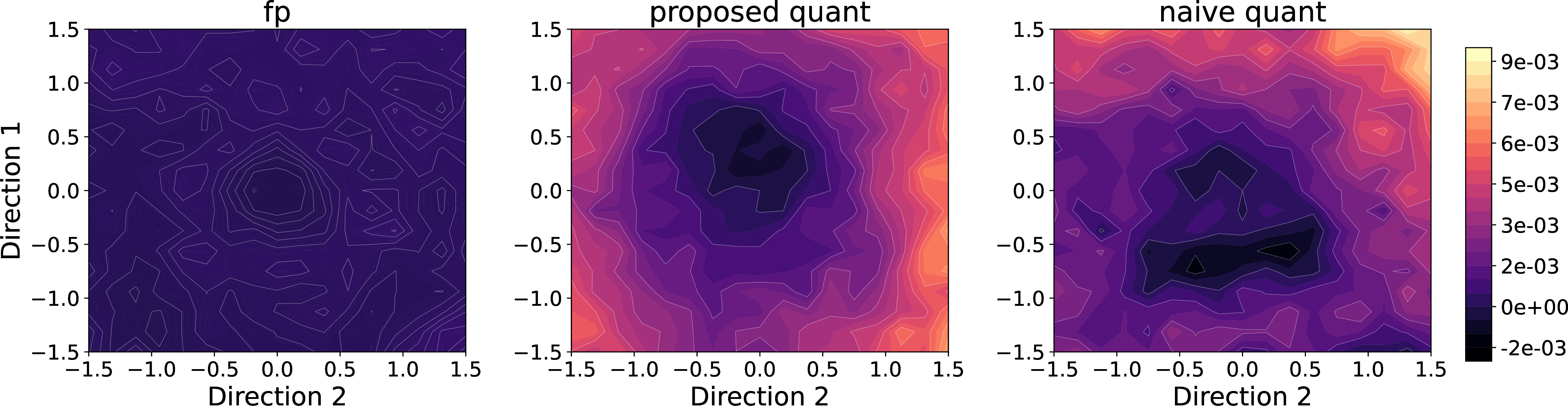
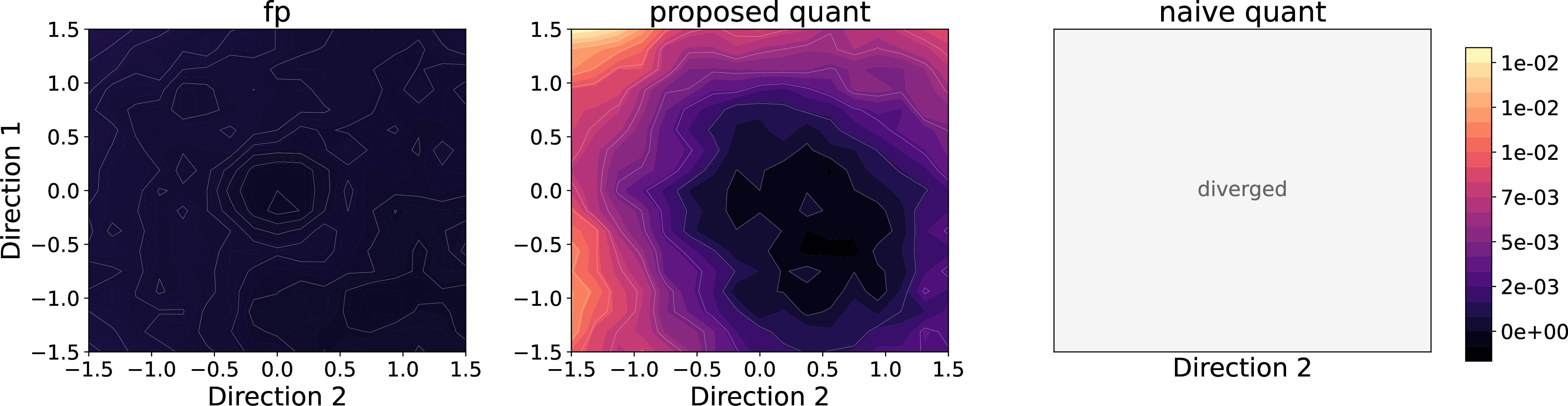
Figure 10: Loss landscape comparison across four training steps (arranged vertically from top to bottom: 32, 384, 512, 672). Each subfigure follows a three-column layout: Column 1 = High-precision baseline; Column 2 = Our full-stack framework; Column 3 = Naive NVFP4 baseline. For the 672-step subfigure (bottommost), Column 3 is marked as derived due to training collapse..
14 Appendix: Model Architecture and Training Configuration Details↩︎
Table ¿tbl:tab:model95arch? and Table [tbl:tab:training95hparams] provide supplementary details on the model architecture and training hyperparameters used in the experiments described in Section 4.