WPG-MoE: Weak-Prior-Guided Dense Mixture-of-Experts for User-Level Social Media Depression Detection
July 05, 2026
Abstract
Online social media posts provide scalable signals for early depression screening, and recent studies mainly improve pre-classification evidence through risk-post selection, symptom grounding, and clinically informed feature construction. However, these screening-stage designs often leave final decisions to a single detector, overlooking how users heterogeneously express depressive risk after screening. A monolithic classifier must average across heterogeneous users, which may dilute localized evidence and cause misclassification, especially for non-self-disclosing users. To address this issue, we propose WPG-MoE, a weak-prior-guided dense mixture-of-experts framework built on a shared large language model (LLM) backbone. WPG-MoE derives user-level weak semantic priors to softly route users to experts matched to different evidence layouts. We formulate this process as learning using privileged information (LUPI): rich LLM-extracted structured evidence guides training-time routing, while inference retains only Patient Health Questionnaire-9 (PHQ-9) template screening and the deployable backbone. Experiments on Chinese and English datasets show that WPG-MoE outperforms strong baselines with interpretable routing behavior.
1 Introduction↩︎
Depression affects an estimated 332 million people worldwide, yet treatment coverage and minimally adequate care remain limited [1], [2]. Social media histories therefore provide scalable early-identification signals, as [3] showed for depression detection from naturalistic user traces [4]–[11].

Recent work improves user-level social media depression detection with complete-history modeling and clinically structured evidence: multimodal fusion, user-post summarization, symptom-aware temporal modeling, capsule-style aggregation [5], [12]–[16], Patient Health Questionnaire-9 (PHQ-9) or psychiatric-scale guidance [17]–[19], and large language model (LLM)-based annotation, summarization, retrieval, or explanation for clinical evidence [20]–[23]. Yet final predictors across pretrained language models (PLMs), sentence-embedding pipelines, capsule models, tree classifiers, and retrieval-augmented LLM agents still make one decision after screening.
The bottleneck is post-screening heterogeneity, not evidence retrieval. Depressed users reveal risk through overlapping structures: diagnoses or medication, sustained symptoms, or a few high-intensity posts amid otherwise irrelevant histories [24]. These are evidence structures, not hard clinical subtypes. Figure 1 illustrates the mismatch: after screening, a flat detector compresses heterogeneous signals into one representation and boundary. This averaging can dilute localized evidence and obscure weaker non-self-disclosure patterns, motivating dense conditional specialization with soft routing, not hard partitioning.
Mixture-of-experts (MoE) naturally supports this specialization, but task-loss-driven routing can be fragile in noisy mental-health settings. It can favor generic correlations over clinically meaningful evidence patterns [25]–[28]. We guide routing with weak priors from clinical cues, encouraging specialization around self-disclosure, episode-supported evidence, and sparse high-risk evidence.
We instantiate this as WPG-MoE, a Weak-Prior- Guided dense Mixture-of-Experts framework for user-level social media depression detection. WPG-MoE softly routes users to evidence-matched experts over a shared LLM backbone. Because the strongest priors come from external LLM-extracted structure useful in training but costly at deployment, we cast WPG-MoE as learning using privileged information (LUPI) [29]: privileged evidence constructs training-time priors and evidence blocks, while inference keeps only deployable PHQ-9 screening, the shared backbone, and history-level signals. Experiments on Chinese and English datasets show improved prediction and interpretable routing. In summary, our contributions follow:
We identify post-screening evidence heterogeneity as a failure mode in user-level social media depression detection.
We introduce WPG-MoE, which softly routes users to experts with clinically grounded weak priors instead of hard subtype labels.
We cast weak-prior-guided routing as LUPI: LLM-derived structure is training-only, while inference stays deployable through shared backbone, not external annotation pipelines.
2 The Approach↩︎
2.1 Problem Definition↩︎
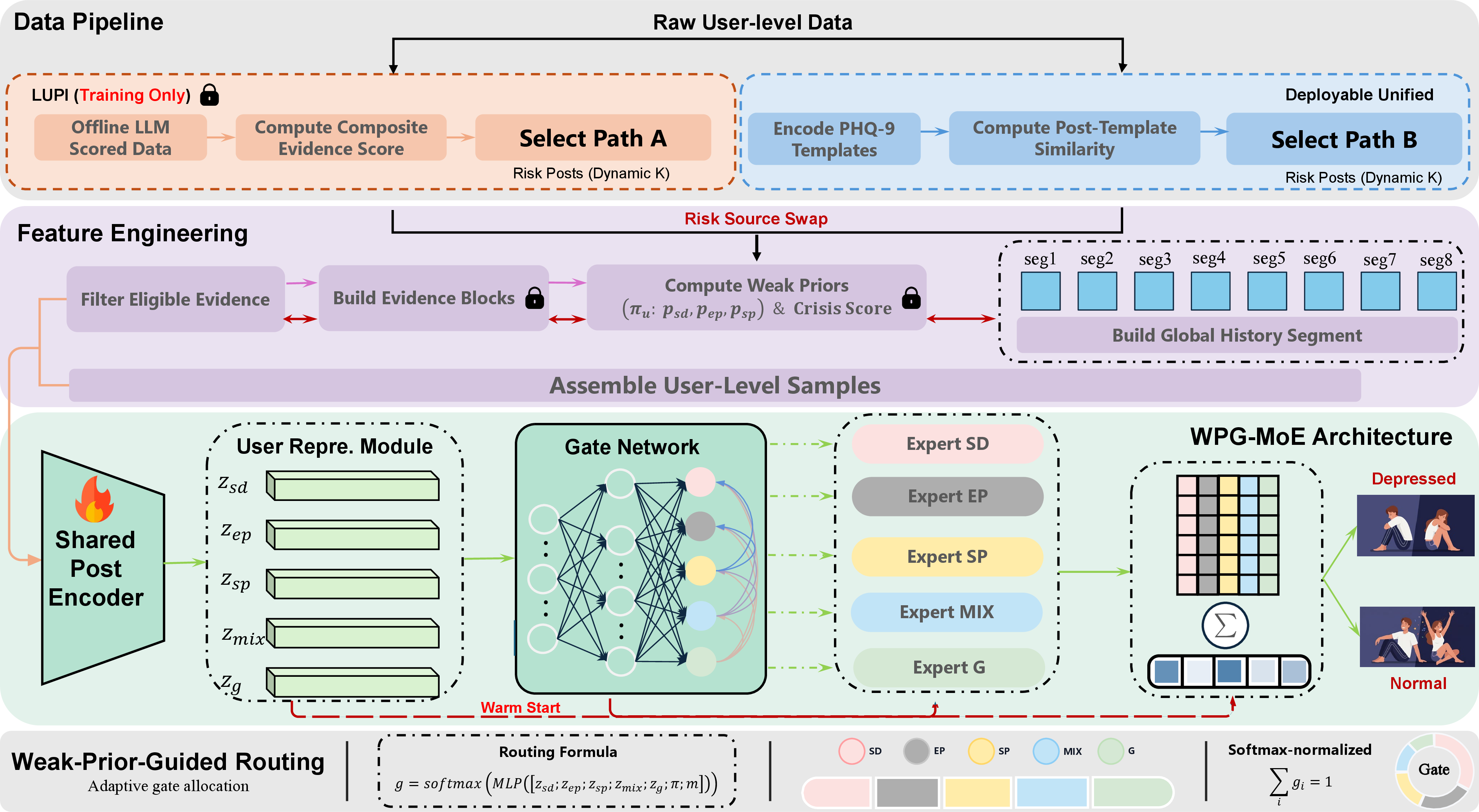
We study user-level textual depression detection. Given a user’s chronological posts \(P=\{p_1,\ldots,p_n\}\) and binary label \(y \in \{0,1\}\), the task is to learn a predictor outputting a user-level decision \(\widehat{y}\): \[\widehat{y} = \mathcal{F}(P).\] WPG-MoE uses privileged training and deployable inference: structured evidence supervises training and routing; inference uses deployable textual signals. Figure 2 summarizes this pipeline.
2.2 Dual-Path Evidence Construction↩︎
Construction follows the training–deployment gap: privileged structure guides learning; PHQ-9 screening remains the inference interface.
We use two text-only risk-post paths: training-only Path A from offline evidence scores and deployable Path B from PHQ-9 screening. Both produce candidate set \(R\), combined with history \(H\) for evidence-centric prediction \(\widehat{y}=f(R,H)\). Privileged training uses \(R^{A}\), whereas deployable inference uses \(R^{B}\). Figure 2 links both to prior induction, routing, and prediction.
2.2.0.1 Path A:
Path A uses training-only structured signals from an offline LLM [30]. The Qwen3-max API scores 909,794 posts from SWDD [15], Twitter [5], and eRisk25 [31]. Each post receives symptom, crisis, anchor, duration, confidence, and self-evidence attributes, then privileged post score \(c_i\): \[\begin{align} c_i = \mathrm{Score}_A\big(&\phi_{\mathrm{sym}}(p_i), \phi_{\mathrm{crisis}}(p_i), \phi_{\mathrm{anchor}}(p_i), \\ &\phi_{\mathrm{dur}}(p_i), \phi_{\mathrm{conf}}(p_i), \phi_{\mathrm{self}}(p_i)\big). \end{align}\] The \(\phi\) terms denote six LLM-derived attributes. \(\mathrm{Score}_A(\cdot)\) maps them to a \([0,1]\) scalar from symptom strength/coverage, crisis severity, anchor presence, duration support, confidence, and explicit self-evidence. Ranking by \(c_i\) yields \(R^{A}\) for auxiliary supervision/weak priors; the external scorer remains separate from the deployable backbone. A blinded human audit validates these fields: A/B agreement is substantial (\(\kappa=0.671\)–\(0.709\)), Qwen-to-adjudicated F1 exceeds 0.80 on main fields, and user-level layout reaches \(\kappa=0.654\) against adjudicated labels (Appendix 7.1).
2.2.0.2 Path B:
At inference, posts are scored against symptom templates. Let \(d \in \{1,\ldots,D\}\) index the \(D\) PHQ-9 symptom dimensions, and \(\mathcal{T}_d\) be the template set for dimension \(d\); Appendix 7.2 lists the templates. The template screener computes \[\begin{align} s_{i,d} &= \max_{q \in \mathcal{T}_d} \cos(\mathrm{Enc}_s(p_i), \mathrm{Enc}_s(q)), \\ r_i &= \mathrm{Score}_B(\{s_{i,d}\}_{d=1}^{D}), \end{align}\] where \(s_{i,d}\) is the maximum similarity between \(p_i\) and dimension \(d\)’s templates, and \(\mathrm{Score}_B(\cdot)\) pools dimension-wise similarities into deployable risk score \(r_i\). Candidates are selected dynamically: \[\begin{align} K &= \mathrm{Budget}(|P|), \\ R^{B} &= \mathrm{TopK}_{K}(\{r_i\}_{i=1}^{n}). \end{align}\] \(K\) is the candidate budget, and \(\mathrm{Budget}(\cdot)\) is history-length-aware. Following E2-LPS [19], the nominal evidence-post screening ratio is 12.5%, with a floor for short histories. The shared backbone encodes candidates for user-level routing and prediction.
During training, routing and evidence scoring see Path-B signals alongside privileged Path A. Table 1 summarizes four perturbations.
| Mechanism | Rate | Meaning / role |
|---|---|---|
| Risk Source Swap | 0.5 | Swaps Path-A and Path-B candidate sources so training also sees deployable risk-post quality. |
| META Dropout | 0.5 | Masks privileged [META] cues so post encoding does not depend on LLM-side annotations. |
| Episode Block Dropout | 0.4 | Removes privileged evidence blocks so the episode view can fall back to deployable risk-post evidence. |
| Prior Dropout | 0.3 | Zeros weak priors so routing remains usable when prior cues are absent at test time. |
3pt
2.3 Weak-Prior-Guided User Modeling↩︎
Weak-prior modeling links screened evidence to conditional specialization, mapping privileged layouts to routing tendencies and views.
2.3.0.1 Weak priors from coarse evidence tendencies and blocks.
Post-screening heterogeneity has three soft layouts: explicit self-disclosure, episode-supported evidence, and sparse high-risk evidence. Explicit self-disclosure, common in mental-health self-reports, is modeled separately [32]–[35]. Episode-supported evidence follows PHQ-9-style screening, but social media histories are too sparse/irregular for rigid two-week rules [36]–[41]; we keep eligible first-person evidence posts above a composite-score threshold and merge adjacent ones into temporal blocks \(B\). Sparse high-risk evidence captures users with only a few isolated but intense signals, observed in post-level monitoring and symptom-detection work [42]–[44]. From privileged posts \(R^{A}\) and blocks \(B\), we derive \(\pi=[\pi_{\mathrm{self}}, \pi_{\mathrm{epis}}, \pi_{\mathrm{sparse}}]\), whose entries summarize self-disclosure, episode-supported evidence, and sparse high-risk evidence: \[\pi = [\pi_{\mathrm{self}},\, \pi_{\mathrm{epis}},\, \pi_{\mathrm{sparse}}] = \mathrm{Prior}(R^{A}, B).\] \(\mathrm{Prior}(\cdot)\) scores self-disclosure from self-claims, anchors, and confidence in \(R^{A}\); episode support from the strongest block in \(B\); and sparse evidence when neither tendency dominates and few high-scoring posts remain. The audited cues support soft routing, not hard labels.2 In parallel, history is partitioned into eight chronological segments \(\{P^{(j)}\}_{j=1}^{8}\). Segment encoder \(\mathrm{SegEnc}(\cdot)\) mean-pools shared post encodings into \(u^{(j)}\); the temporal aggregator \(\mathrm{TAgg}(\cdot)\) applies self-attention over the eight segment vectors to produce global history representation \(H\): \[\begin{align} u^{(j)} &= \mathrm{SegEnc}(P^{(j)}), \qquad j=1,\ldots,8, \\ H &= \mathrm{TAgg}\!\big(u^{(1)}, \ldots, u^{(8)}\big), \end{align}\] This branch retains broad mood evolution more cheaply than encoding all posts [15], [41].
2.3.0.2 Multi-view user representation.
We use five views: three tendency-specific channels for self-disclosure, episode-supported evidence, and sparse high-risk evidence; a mixed cross-channel view; and a global residual-history view. The shared LLM encoder represents each candidate post with its last non-padding token’s final-layer hidden state. The user module builds \(\{z_1, z_2, z_3, z_4, z_5\}\): three attention-pooled channel views, a mean-pooled mixed risk-post view, and a global view combining temporal self-attention and projected summary statistics. We collect crisis and history statistics into metadata vector \(m\). A five-expert dense MoE predicts gate weights \(g=[g_1,\ldots,g_5]\), where \(e_k\) is the \(k\)-th expert output and \(h\) the fused state: \[\begin{align} g &= \mathrm{softmax}\Big(\mathrm{MLP}([z_1; z_2; z_3; z_4; z_5; \pi; m])\Big), \\ e_k &= \mathrm{Expert}_k([z_k; m]), \\ h &= \sum_{k=1}^{5} g_k\, e_k, \end{align}\] Weak priors act as soft routing hints rather than hard subtype labels.
2.4 Prediction and Learning↩︎
Learning preserves the LUPI boundary: privileged evidence supervises training, while deployable posts define the routed state used at inference.
Evidence scoring. Given candidate post representation \(x_i\), the fused user state \(h\), and the gate vector \(g\), the auxiliary scoring head computes training-time post score: \[a_i = \sigma\Big(\mathrm{MLP}([x_i; h; g])\Big).\] Here \(a_i \in (0,1)\) supervises training-time evidence.
Training objective. We jointly optimize user prediction, routing, and evidence supervision: \[\mathcal{L} = \mathcal{L}_{\mathrm{cls}} + \alpha \mathcal{L}_{\mathrm{route}} + \beta \mathcal{L}_{\mathrm{evi}} + \gamma \mathcal{L}_{\mathrm{bal}} + \delta_t \mathcal{L}_{\mathrm{ent}}.\] Here \(\delta_t\) is the training-step-dependent entropy coefficient. \(\mathcal{L}_{\mathrm{cls}}\) is the user-level classification loss, \(\mathcal{L}_{\mathrm{route}}\) aligns the first three expert gates with confident weak priors, \(\mathcal{L}_{\mathrm{evi}}\) supervises evidence scores on depressed users with silver labels, \(\mathcal{L}_{\mathrm{bal}}\) discourages expert imbalance, and \(\mathcal{L}_{\mathrm{ent}}\) controls routing sharpness through decayed entropy.
Inference. Training applies risk-source swap/dropout to metadata, evidence blocks, weak priors, and candidate posts, exposing gates to privileged and deployable inputs. At inference, removing Path A/privileged annotations leaves only template-screened posts, shared backbone, eight-segment summaries, and user statistics. Appendix 7.5 reports rules and hyperparameters for candidate construction, weak-prior induction, routing, and training.
3 Experimental Settings↩︎
3.1 Datasets, Label Audit, and Controlled Protocol↩︎
We use three text-only user-level depression-detection datasets: SWDD (Chinese; [15]), the Twitter depression dataset (English; [5]), and eRisk25 (English; [31]). All runs use a unified stratified \(80/10/10\) holdout for within- and cross-dataset comparison, following recent user-level depression-detection practice with consistent partitions [16], [17], [19], [45]; the protocol supports controlled, not leaderboard, comparison.
3.1.0.1 SWDD label audit.
SWDD’s raw self-report flag (self_reported) contains label errors, so all SWDD experiments use the corrected split unless otherwise noted. Candidate corrections from mismatch screens were manually reviewed per user before finalizing
corrected counts. The audit procedure, corrected class distribution, and representative cases appear in Appendix 7.7 and Table 11. Table 2 summarizes the final dataset versions.
| Statistic | SWDD | eRisk25 | |
|---|---|---|---|
| No. of users (Dep.) | 3,711 | 1,218 | 102 |
| No. of users (Ctrl.) | 19,526 | 1,273 | 807 |
| No. of posts (Dep.) | 643,139 | 196,268 | 70,387 |
| No. of posts (Ctrl.) | 3,357,273 | 700,320 | 348,803 |
| Avg. posts per user (Dep.) | 173.3 | 161.1 | 690.1 |
| Avg. posts per user (Ctrl.) | 171.9 | 550.1 | 432.2 |
| Users split | 18,588 / 2,324 / 2,325 | 1,992 / 249 / 250 | 726 / 91 / 92 |
2pt

3.2 Experimental Protocols↩︎
All experiments use unified holdout splits in Table 2. Models train on one source and test in-domain or transfer without changes. We report five-run mean recall, F1, area under the receiver operating characteristic curve (AUROC), and area under the precision-recall curve (AUPRC). Recall and F1 measure thresholded detection, AUROC measures threshold-free ranking, and AUPRC targets imbalanced settings such as SWDD and eRisk25.
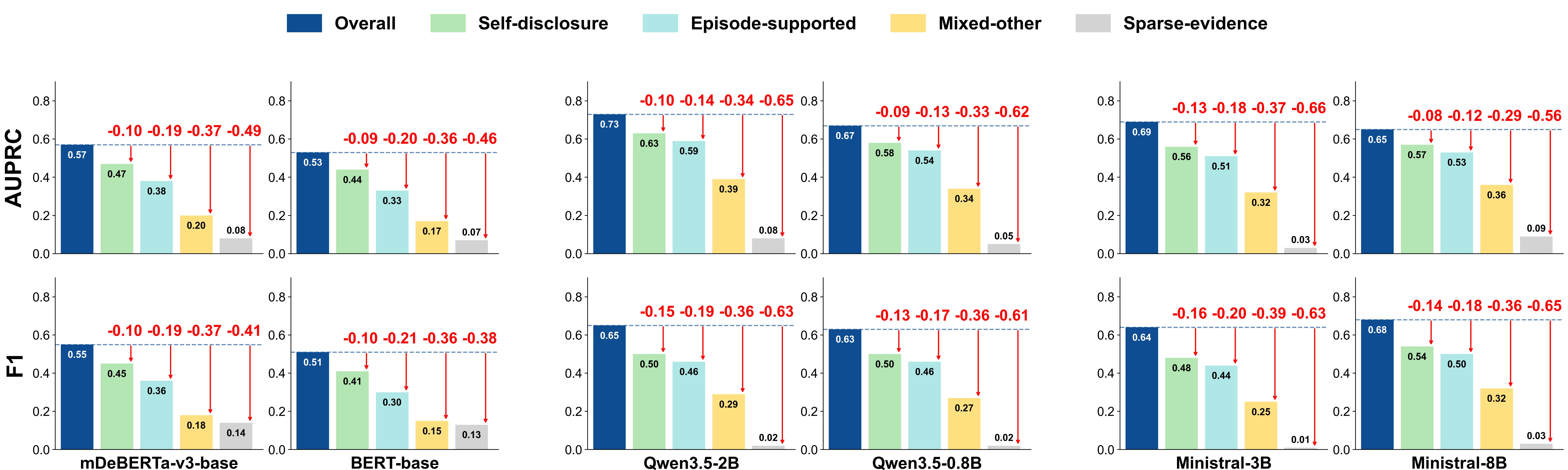
We also test whether post-screening evidence layouts yield stable differences without weak-prior-rule slice sources. The diagnostic uses blinded human evidence-layout labels: 360 depressed users from SWDD, Twitter, and eRisk25 paired with 1,800 fixed same-dataset controls. Because sparse/mixed layouts are rare within datasets, we pool three datasets and omit per-dataset layout-prevalence estimates. Appendix 7.8 reports complementary large-scale rule-derived SWDD diagnostic and controlled-mixing counts. For backbone replacement, Base is a raw backbone classifier and Ours denotes same-backbone WPG-MoE. We report mDeBERTa-v3-base [46], Qwen3.5-2B [47], and Ministral-3B [48]; Appendix 7.9 adds BERT-base [49], Qwen3.5-0.8B [47], and Ministral-8B [48]. Unless replaced, WPG-MoE uses Qwen3.5-2B as shared encoder; Path A is separate and used only for source-train depressed users, while dev/test and transfer targets use raw histories and Path B.
3.3 Baselines and Metrics↩︎
We compare WPG-MoE with seven baselines in four families: PHQ-9-grounded pattern matching [17], psychiatric-scale-guided risky-post screening [18], [19], symptom-structured representation learning [16], and LLM-assisted clinically informed detection [21]. Detailed baseline notes are given in Appendix 7.11.
4 Results and Analyses↩︎
4.1 Slice-Level Heterogeneity↩︎
| Scope | Users | Raw agr. | \(\kappa\) | \(\alpha\) | Adj. |
|---|---|---|---|---|---|
| SWDD | 180 | 0.817 | 0.735 | 0.738 | 33 |
| 120 | 0.792 | 0.690 | 0.694 | 25 | |
| eRisk25 | 60 | 0.767 | 0.641 | 0.650 | 14 |
| Overall | 360 | 0.800 | 0.707 | 0.708 | 72 |
2pt
To test whether screened data contains evidence heterogeneity affecting detector performance before WPG-MoE, we evaluate six flat detectors from three model families (two variants each) on a blinded human evidence-layout diagnostic. Slices are assigned from raw, unscored packets under pre-specified annotation guidelines, rather than rule-derived categories. The diagnostic pools 360 depressed users from SWDD, Twitter, and eRisk25 with the same 1,800 controls and validation-set thresholding per slice; sparse/mixed cases are rare, motivating cross-dataset pooling. Table 3 reports raw agreement 0.800, Cohen’s \(\kappa=0.707\), and Krippendorff’s \(\alpha=0.708\); Appendix 7.8 gives sampling, packet visibility, labels, guidelines, and the larger corrected-SWDD tendency/block diagnostic. Figure 3 shows stable degradation across model families: self-disclosure and episode-supported users are easier, whereas mixed/other and sparse-evidence users are more difficult. The same ordering in the larger diagnostic further indicates evidence layout is tied to detection difficulty.
4.2 Overall Results and Generalization↩︎
We evaluate within-dataset detection and transfer under identical partitions. Table ¿tbl:tab:cross-dataset-target-tuned? compares WPG-MoE with seven baselines under the unified holdout for method comparability, not leaderboard claims. WPG-MoE gives the strongest in-domain results and keeps advantages on most cross-dataset Recall, F1, and AUPRC cells. Transfer gains are clearest when SWDD is source, consistent with its larger supervision scale. Twitter-trained models remain competitive, while eRisk25-trained models leave a few off-diagonal AUROC cells matched or slightly exceeded by clinically guided baselines, suggesting robust transfer needs enough source supervision under shift. Appendix 7.12 reports Ours across five seeds; F1 and AUPRC standard deviations stay within 0.0063–0.0083 and 0.0088–0.0113 across the nine train\(\rightarrow\)test cells.
3pt width=,center

These results use Qwen3.5-2B as the default deployable backbone. To separate architecture effects from backbone choice, Table [tab:backbone-replacement] compares each Base classifier with matched-backbone WPG-MoE on in-domain cells; Appendix 7.9 gives the complete train\(\rightarrow\)test matrix and compact-LLM variants. Ours improves over the corresponding Base setting for mDeBERTa-v3-base, Qwen3.5-2B, and Ministral-3B, tying the gain to WPG-MoE rather than selecting one stronger pretrained model.
4.3 Controlled Mixing and Routing Analyses↩︎
Routing analysis tests whether layouts act as compatible tendencies, not isolated classes, via slice mixing and train\(\rightarrow\)test gate allocation.
4.3.0.1 Controlled mixing and dense routing.
Slice analysis shows stable layout differences, but layouts need not be isolated classes. To test shared depressive signal, we start from one target slice and add positives from other slices during training. Figure 4 shows target-slice AUPRC and F1 usually hold or improve, most clearly when self-disclosure users enter episode-supported training. This supports dense MoE: overlapping evidence tendencies enable expert-signal sharing while retaining tendency-aware specialization.
4.3.0.2 Gate allocation analysis.
Figure 5 reports average training gates for five WPG-MoE expert views on SWDD, Twitter, and eRisk25: self-disclosure receives the largest weight, reflecting strong weak-prior self-report cues, while episode, mixed, and global experts remain active, avoiding reliance only on explicit diagnosis or medication mentions. Figure [fig:test-gate-allocations] reports test-time allocations; train\(\rightarrow\)test variation suggests gates adapt evidence mixtures to target users rather than follow fixed patterns. Dense-MoE weights describe expert-view contributions, not evidence-type assignments.
4.4 Ablation Analysis↩︎
Table [tab:cross-dataset-ablation] ablates links among privileged evidence, deployable screening, and routing on in-domain cells; the complete train\(\rightarrow\)test ablation matrix appears in Appendix 7.10. Removing dense MoE gives the largest loss, confirming one shared state is too coarse. Path A and DP dropout are next most important, while weak priors and route loss yield smaller but stable drops, indicating that they shape expert allocation rather than act as standalone predictors.
Figure 6:  .
.
4.5 Case Study↩︎
To examine whether WPG-MoE better handles difficult evidence layouts than previous screening-based detectors, Figure 6 compares two anonymized SWDD cases. For privacy, posts are paraphrased to preserve core meaning while removing identifiers, user details, timestamps, original sentence structure, and exact identifiable wording. The sparse-evidence user shows ordinary posts with few isolated, intense depressive cues; user-level DeCapsNet weakens them, yielding a missed/weak output. WPG-MoE detects them by keeping sparse, mixed, and global views active. For the episode-supported user, sleep disturbance, low mood, and withdrawal recur without a decisive post. DeCapsNet fragments this pattern; WPG-MoE emphasizes episode-supported/global experts for correct output. These cases show WPG-MoE preserves evidence-layout heterogeneity single-path screeners tend to blur.
5 Related Work↩︎
User-level depression detection from social media has moved from holistic profile modeling to evidence-oriented user representation [3], [5], [13], [50], [51]. One line of work reduces noisy posting histories by selecting or summarizing indicator posts, modeling temporal symptom signals, or fusing heterogeneous modalities [12]–[15], [52]–[54]. Another line grounds prediction in clinically meaningful structures, including PHQ-9 questionnaires, psychiatric-scale screening, and symptom capsules [16]–[19], [55], [56]. Recent LLM-based systems further extract DSM-style symptoms, mood courses, clinical evidence, or questionnaire responses for interpretable screening [20]–[23], [30], [57]–[63]. These methods improve evidence selection and interpretability, but most still compress the selected evidence into a single user representation or pass it to a single detector, which can blur sparse cues and episode-level patterns across heterogeneous users.
Our work is also related to conditional computation. Mixture-of-experts (MoE) models support specialization across examples, tasks, or modalities [25], [26], [64]–[66], and have recently been explored for mental-health prediction from textual and non-textual social-media signals [27], [28]. However, existing mental-health MoE methods mainly treat experts as representation, language, or modality specialists rather than routing them with clinically structured evidence layouts. Learning using privileged information (LUPI) provides a complementary view: richer signals can guide training even when they are unavailable at deployment [29], [67], [68]. WPG-MoE combines these threads by using LLM-derived Path-A fields as training-only, layout-aware weak routing priors, while inference keeps PHQ-9 screening and a shared backbone without external LLM processing.
6 Conclusion↩︎
We study user-level depression detection with post-screening heterogeneity. WPG-MoE combines dual-path evidence, weak-prior routing, and dense experts to reduce shared-detector averaging under LUPI, with PHQ-9 screening retained at inference. Chinese/English experiments show gains over strong baselines with interpretable routing. Slice and case analyses further show this gain comes from preserving sparse and episode-supported cues under PHQ-9-only inference.
7 Appendix↩︎
7.1 Weak-Prior Scoring Audit↩︎
We conduct a blinded human audit to assess whether the Qwen-derived structured fields used by Path A provide reliable weak-prior signals. Three trained computer-science student annotators participated after guideline training and a qualification test. Annotators A and B independently labeled anonymized samples, while Annotator C adjudicated only their disagreements. The annotators had access to the anonymized text and annotation guideline, but not to Qwen scores, model predictions, or experimental outcomes. Table 4 summarizes the stratified audit sample.
7.1.0.1 Annotator recruitment and project participation.
The three annotators were recruited from computer-science graduate students with prior coursework or research experience in NLP annotation. Before annotation, they completed guideline training and a qualification test. Annotation was conducted as part of a supervised research project. The task did not require annotators to make clinical judgments; they labeled only predefined textual evidence categories from anonymized packets. Annotators were allowed to pause or stop annotation if they felt uncomfortable with mental-health-related content.
The audit sample is designed to cover both frequent and difficult evidence patterns rather than only high-confidence self-disclosure posts. Because the three datasets differ substantially in user count and history length, we keep all 102 eRisk25 depressed users and sample larger but still tractable subsets from Twitter and SWDD. Twitter and SWDD users are stratified by posting volume, maximum Path-A composite score, and preliminary evidence layout. Within each selected user, posts are chosen to include top-ranked evidence, self-disclosure or clinical-anchor posts, symptom/crisis/duration cues, low-score controls, and time-random context posts; eRisk25 additionally includes early- and late-history random posts because its user histories are much longer. The three tables below separate sample coverage, binary post-level reliability, and non-binary/user-level reliability, so the audit design and the scorer quality are inspected independently.
| Dataset | Users | Posts | Posts/User |
|---|---|---|---|
| eRisk25 | 102 | 1,020 | 10 |
| 200 | 1,600 | 8 | |
| SWDD | 400 | 3,200 | 8 |
| Total | 702 | 5,820 | – |
0pt
| Field | Agr. | \(\kappa\) | P | R | F1 |
|---|---|---|---|---|---|
| First-person | 0.885 | 0.671 | 0.780 | 0.880 | 0.827 |
| Literal self-evidence | 0.893 | 0.689 | 0.765 | 0.875 | 0.816 |
| Any symptom | 0.901 | 0.693 | 0.770 | 0.890 | 0.826 |
| Clinical anchor | 0.913 | 0.709 | 0.750 | 0.860 | 0.801 |
| Duration/frequency | 0.888 | 0.676 | 0.780 | 0.880 | 0.827 |
| Crisis any | – | – | 0.780 | 0.870 | 0.822 |
| Valid evidence | 0.890 | 0.681 | 0.760 | 0.900 | 0.824 |
0pt
| Target | Metric | A/B | Qwen vs. Human |
|---|---|---|---|
| Symptom dimensions | micro/macro-F1 | 0.781 / 0.675 | 0.806 / 0.691 |
| Symptom strength | weighted \(\kappa\) | 0.692 | 0.701 |
| Crisis level | weighted \(\kappa\) | 0.672 | 0.685 |
| Functional impairment | weighted \(\kappa\) | 0.684 | 0.664 |
| User evidence layout | exact/\(\kappa\)/macro-F1 | 0.754 / 0.683 / 0.692 | 0.713 / 0.654 / 0.665 |
5.5pt
For the PHQ-9-aligned symptom_vector, we evaluate three derived targets: whether any symptom evidence is present (P/R/F1), which PHQ-9 dimensions are expressed (micro/macro-F1), and the overall ordinal symptom strength (weighted \(\kappa\)). Cohen’s \(\kappa\) is chance-corrected agreement; weighted \(\kappa\) additionally penalizes larger 0–3 disagreements. Across the audited fields, A/B
agreement is substantial but not perfect, which is expected for short, informal, and sometimes ambiguous social-media text. Qwen-to-human scores remain consistently high for the binary fields and moderate-to-strong for multi-label or ordinal targets,
supporting their use as reliable training-time weak-prior signals rather than as clinical labels or deploy-time inputs.
7.2 PHQ-9 Symptom Template Inventory↩︎
Path B groups template queries by the nine PHQ-9 symptom dimensions: anhedonia, depressed mood, sleep disturbance, fatigue, appetite change, guilt or worthlessness, concentration difficulty, psychomotor change, and self-harm or suicidal ideation. Each template is a short natural-language query used for semantic-similarity screening, not a diagnostic questionnaire score. This inventory links the deployable screening branch to the same symptom vocabulary used by Path A, while avoiding any training-only structured scorer at inference time.
7.3 User-Type Reference Audit↩︎
We next audit the user-level evidence-layout labels induced from the weak-prior pipeline. This audit differs from the post-level scoring audit above: annotators inspect a complete sampled user packet and assign the dominant evidence layout among self-disclosure, episode-supported, sparse-evidence, and mixed/other. Annotators A and B label each packet independently, and Annotator C adjudicates only A/B disagreements. The resulting labels are used as adjudicated reference categories for checking the weak-prior assignment rule; they are not clinical diagnoses.
| Data | Slice | Avail. | Audit | Bndry. | Posts/U | Rule |
|---|---|---|---|---|---|---|
| SWDD | self-disclosure | 1,815 | 40 | 10 | 173.3 | stratified |
| SWDD | episode-supported | 1,223 | 40 | 10 | 173.3 | stratified |
| SWDD | mixed/other | 650 | 35 | 10 | 173.3 | stratified |
| SWDD | sparse-evidence | 21 | 21 | – | 173.3 | all |
| self-disclosure | 7 | 7 | – | 161.1 | all | |
| episode-supported | 484 | 40 | 10 | 161.1 | stratified | |
| sparse-evidence | 271 | 35 | 10 | 161.1 | stratified | |
| mixed/other | 212 | 35 | 10 | 161.1 | stratified | |
| eRisk25 | episode-supported | 71 | 71 | – | 690.1 | all |
| eRisk25 | sparse-evidence | 5 | 5 | – | 690.1 | all |
| eRisk25 | mixed/other | 5 | 5 | – | 690.1 | all |
1pt
Table 7 shows that the audit covers both high-prevalence slices and rare slices. For rare categories, such as sparse-evidence users in SWDD and eRisk25, we audit all available users; for larger categories, stratified sampling retains boundary cases to avoid overstating reliability on easy high-margin examples. This design makes the reference set suitable for assessing whether weak-prior grouping remains stable under realistic ambiguity.
| Scope | \(N\) users | Raw agr. | Cohen’s \(\kappa\) | Kripp. \(\alpha\) | Adj. by C |
|---|---|---|---|---|---|
| Overall | 334 | 0.802 | 0.705 | 0.754 | 66 |
| SWDD | 136 | 0.801 | 0.703 | 0.752 | 27 |
| 117 | 0.803 | 0.708 | 0.757 | 23 | |
| eRisk25 | 81 | 0.803 | 0.701 | 0.751 | 16 |
1.8pt
The agreement results in Table 8 are consistent across datasets despite differences in language, platform, and history length. Overall A/B agreement reaches 0.802, with Cohen’s \(\kappa=0.705\) and Krippendorff’s \(\alpha=0.754\), indicating substantial chance-corrected reliability for a four-way evidence-layout judgment. The 66 adjudicated disagreements are concentrated in boundary cases, where direct self-disclosure, repeated episode evidence, and mixed evidence can overlap; this is precisely why WPG-MoE uses these categories as soft routing tendencies rather than fixed clinical subtypes.
3pt
@lrrrrr@ Ref. slice & Sup. & P & R & F1 & Confusion
self-disclosure & 47 & 0.609 & 0.596 & 0.602 & episode-supported
episode-supported & 151 & 0.861 & 0.861 & 0.861 & mixed/other
sparse-evidence & 61 & 0.613 & 0.623 & 0.618 & mixed/other
mixed/other & 75 & 0.827 & 0.827 & 0.827 & episode-supported
Overall & 334 &
Table ¿tbl:tab:appendix-user-type-assignment? indicates that the deterministic weak-prior assignment rule recovers the adjudicated reference labels with 0.772 accuracy and 0.727 macro-F1. The strongest alignment appears for episode-supported and mixed/other users, while self-disclosure and sparse-evidence are more often confused with neighboring layouts. These errors are interpretable: self-disclosure posts can also occur inside repeated episodes, and sparse high-risk users often border on mixed evidence when a few additional moderate posts are present. The audit therefore supports the quality of the weak-prior grouping while reinforcing the paper’s design choice to use it as soft privileged supervision rather than as a hard target at inference time.
7.4 User-Type Examples↩︎
Table 9 shows one representative eRisk user for each coarse evidence tendency. To avoid surfacing raw user handles, we replace the original identifiers with E1–E3 while keeping the underlying post excerpts and derived weak-prior patterns unchanged. The purpose of these examples is to make the routing targets in Section 2 inspectable: the same depressed label can be supported by a direct self-report, a temporally repeated episode, or a small number of intense posts. The rows therefore illustrate evidence layouts rather than clinical subtypes, and they explain why WPG-MoE uses soft tendency-specific views together with a global fallback expert.
| Type | Representative excerpts | Why it matches the channel |
|---|---|---|
| Self-disclosure (E1) | “I am finally taking a firm decision to get help after 10 years of major depression …” | This user contains direct first-person disclosure of diagnosis and treatment seeking. The self-disclosure prior is therefore high, while the user has only a short supporting block, so the key signal is explicit self-report rather than long-range aggregation. |
| Episode-supported evidence (E2) | “My PHQ-9 is down to a 20 …it was 25+ for the last two years”; “2 Day migraine …Depression x10 …I just want to die.” | This user has three evidence blocks spanning 29, 48, and 24 days. The decision is supported by repeated symptoms across temporally linked posts rather than by a single disclosure post, which is exactly the pattern targeted by the episode-supported channel. |
| Sparse high-risk evidence (E3) | “I just feel like vanishing right now”; “My mother doesn’t believe that I’m depressed despite having been diagnosed with it …” | This user has only one short evidence block and relatively few risk posts, but several of them are intense enough to raise the sparse-evidence prior. The key signal is concentrated in a small number of high-impact posts rather than in a dense episode-like cluster. |
5pt
7.5 Implementation Details and Hyperparameters↩︎
This subsection records the code-level choices that instantiate the operators in Section 2. We include only settings that affect reproducibility; the external Path-A annotation schema is shown separately in Appendix 7.6.
7.5.0.1 Model size and compute budget.
The default WPG-MoE configuration uses Qwen3.5-2B as the deployable backbone (approximately 2B parameters). Across backbone-replacement and baseline experiments, we also evaluate BERT-base (approximately 110M parameters), mDeBERTa-v3-base (approximately 278M parameters), Qwen3.5-0.8B, Ministral-3B, and Ministral-8B. The measured training time below refers to the default Qwen3.5-2B WPG-MoE runs. Training uses data parallelism on four NVIDIA A100 GPUs. One source-dataset run takes about 4 hours for SWDD and about 2 hours for Twitter or eRisk25.
| Component | Implementation setting |
|---|---|
| Template encoder | gte-small-zh for SWDD; all-MiniLM-L6-v2 for Twitter/eRisk; normalized embeddings. |
| Backbone | Qwen3.5-2B in the main runs; automatic pooling uses the last token. |
| Candidate/history caps | risk candidates; eight chronological history segments; 60% history coverage; 12 posts per segment in full-parameter Qwen configs. |
| Training perturbations | Risk-source swap 0.5, metadata drop 0.5, block drop 0.4, prior drop 0.3, post drop 0.3; Twitter/eRisk configs use template-source swap 1.0. |
| Optimizer | AdamW; head learning rate \(10^{-4}\); encoder learning rate \(10^{-5}\) in full-parameter Qwen configs; weight decay 0.01; gradient clipping 1.0. |
| Training schedule | Stage-D expert warm start for 3 epochs; Stage-E joint training for up to 3 epochs with validation-F1 early stopping; effective Stage-E batch size 8 in full-parameter Qwen configs. |
| Loss weights | \(\alpha=0.3\), \(\beta=0.2\), \(\gamma=0.15\); entropy weight decays from 0.1 to 0.02 with a cosine schedule. |
| Routing loss | Applied only when the largest weak prior is at least 0.6 and exceeds the second largest by at least 0.1; KL aligns the first three gate weights with normalized weak priors. |
| Balance/entropy losses | Balance uses batch-level importance and sharpened load with temperature 0.1; entropy is added as negative gate entropy to encourage early routing diversity. |
2pt
7.5.0.2 Candidate scores and budgets.
For a user with \(n\) posts, both Path A and Path B keep the top \(K(n)\) posts, where \[K(n)= \begin{cases} \lceil 0.125n \rceil, & n\geq 160,\\ 20, & 20\leq n<160,\\ n, & n<20. \end{cases}\] Path A maps structured LLM fields to a weak evidence ranker, not a tuned post-level classifier. Let \(e_i^A=[q_i,c_i,a_i,d_i,r_i,u_i]\in[0,1]^6\) collect normalized symptom, crisis, clinical-anchor, duration, confidence, and literal self-disclosure cues, where \(q_i\) summarizes PHQ-9 symptom intensity and coverage from \(v_i\in\{0,1,2,3\}^{9}\). We compute \[\begin{align} s_i^A&=\mathrm{clip}_{[0,1]}\!\left((w^A)^\top e_i^A\right),\\ w^A&\geq 0,\qquad \|w^A\|_1=1 . \end{align}\] where \(w^A\) is a fixed symptom-heavy vector, not selected on validation or test targets. The score only constructs training-time weak priors and is removed at inference. Path B embeds each post and the PHQ-9 template inventory with normalized sentence embeddings. For dimension \(d\), the dimension score is the maximum cosine similarity to that dimension’s three templates. The template risk score uses a fixed pooling rule over the strongest PHQ-9 dimensions, \(s_i^B=\mathrm{Pool}_{\mathrm{PHQ}}(\{b_{i,d}\}_{d=1}^{D})\); matched dimensions are retained as lightweight metadata. The final model input uses at most 32 candidate posts in the Qwen full-parameter configurations.
7.5.0.3 Evidence blocks and weak priors.
Evidence blocks are built only for depressed training users with Path-A scores. A post is eligible when it is first-person, literal self-evidence, and passes a fixed weak-evidence threshold. Eligible posts are ordered by timestamp and adjacent posts within a short temporal window are merged. Blocks are scored by monotone pooling over normalized block evidence: \[B=\mathrm{Pool}_{\mathrm{blk}} \bigl(\tilde{n}_b,\tilde{\ell}_b,\tilde{m}_b,d_b,\tilde{f}_b,\bar r_b\bigr),\] where the tilded variables normalize block post count, span, symptom coverage, and impairment; \(d_b\) indicates duration and \(\bar r_b\) is average confidence. Each block stores representative posts, and each user keeps only top-ranked blocks.
The implemented weak prior vector is \(\pi=[\pi_{\mathrm{sd}},\pi_{\mathrm{ep}},\pi_{\mathrm{sp}}]\). The self-disclosure prior averages per-post evidence from current self-claims, clinical anchors, current literal self-evidence, and confidence. The episode-supported prior is computed from the best block using its post count, span, symptom coverage, duration support, and functional impairment. The sparse evidence prior is activated when neither self-disclosure nor episode evidence dominates and the user has only a few high-scoring posts; it combines the top composite scores and average confidence. The crisis score is the maximum Path-A crisis level and is normalized before being passed to the model. At inference time, Path A, episode blocks, weak priors, and crisis annotations are removed; Path B candidates and lightweight statistics remain.
7.5.0.4 Representation and routing.
The shared encoder produces post representations that are aggregated into five views: \(z_{\mathrm{sd}}\) attends over all risk candidates, \(z_{\mathrm{ep}}\) attends over block posts and falls back to risk candidates when blocks are absent, \(z_{\mathrm{sp}}\) attends over the first three risk candidates, \(z_{\mathrm{mix}}\) mean-pools risk candidates, and \(z_g\) applies temporal self-attention to eight global-history segments plus a statistics projection. The attention-pooling modules are separate linear scoring heads, so the three evidence-oriented views learn different pooling weights. The gate is a two-layer MLP with hidden size 256 and dropout 0.1 over \([z_{\mathrm{sd}};z_{\mathrm{ep}};z_{\mathrm{sp}};z_{\mathrm{mix}};z_g;\pi;c;\mathrm{stats}]\). All five experts are evaluated for every user. Each expert receives one view concatenated with a 10-dimensional projected metadata vector and uses Linear\((d+10,512)\), GELU, dropout 0.1, and Linear\((512,256)\), where \(d\) is the encoder hidden size; the MoE state is the dense weighted sum of expert outputs. The auxiliary scoring head maps \([x_i;h;g]\) through an MLP and sigmoid for training-time evidence supervision.
7.6 Training-Time External LLM Scoring Prompt↩︎
Path A is built by an offline single-post scoring script that feeds tweet_index, posting_time, and text into a schema-constrained LLM annotation interface. The repository prompt is written in Chinese; for
readability, we show a faithful English translation below. The structured output is then used for composite post scoring, evidence-block construction, and weak-prior induction. This external prompt defines the training-time privileged scorer only; it is
distinct from the deployable Qwen3.5-2B backbone used in the main model.
System prompt (English translation). You are a data annotation assistant for mental-health research. Your task is post-level evidence extraction, not clinical diagnosis, not PHQ-9 total-score calculation, and not counseling. Judge only from the given post text and rely strictly on explicit textual evidence rather than speculation.
Return the following fields.
first_person(boolean): whether the post is written from the author’s own perspective.literal_self_evidence(boolean): whether the post is a direct self-report rather than quotation, news, jokes, lyrics, metaphor, or third-person discussion.symptom_vector: a 9-dimensional PHQ-9-aligned symptom evidence vector with values in {0,1,2,3}.crisis_level(0/1/2/3): suicide, self-harm, or acute collapse risk.duration: whether the post contains a duration or frequency cue; if a day span is explicit, return it ashint_span_days, otherwisenull.functional_impairment(0/1/2/3): whether the post indicates functional impairment.clinical_context: includesdisease_mention_type={none, generic_topic, self_history, current_self_claim} and a subset ofanchor_types={diagnosis, doctor_visit, psychiatry, hospitalization, medication, follow_up, therapy}.temporality={current, past, recovery, unclear}.confidence(0.0–1.0): confidence that the post contains genuine mental-health evidence rather than quotation, humor, or hearsay.
Constraints. This is single-post evidence extraction rather than user-level diagnosis. The values in symptom_vector denote textual evidence strength rather than PHQ-9 two-week frequency. Absence of evidence means
lack of information, not counter-evidence. The posting_time string must be copied verbatim into the output. Return valid JSON only, with no extra text.
Structured output template.
{
"tweet_index": <int>,
"posting_time": "<original string>",
"first_person": <bool>,
"literal_self_evidence": <bool>,
"symptom_vector": {
"depressed_mood": 0/1/2/3,
"anhedonia": 0/1/2/3,
"sleep": 0/1/2/3,
"fatigue": 0/1/2/3,
"appetite_or_weight": 0/1/2/3,
"worthlessness_or_guilt": 0/1/2/3,
"concentration": 0/1/2/3,
"psychomotor": 0/1/2/3,
"suicidal_ideation": 0/1/2/3
},
"crisis_level": 0/1/2/3,
"duration": {"has_hint": <bool>, "hint_span_days": <int|null>},
"functional_impairment": 0/1/2/3,
"clinical_context": {
"disease_mention_type":
"<one of: none, generic_topic,",
"self_history, current_self_claim>",
"anchor_types": ["diagnosis", "..."]
},
"temporality": "current|past|recovery|unclear",
"confidence": <float>
}
Illustrative scored example.
{
"tweet_index": 17,
"posting_time": "2024-03-12 21:14:05",
"first_person": true,
"literal_self_evidence": true,
"symptom_vector": {
"depressed_mood": 3, "anhedonia": 2, "sleep": 2,
"fatigue": 2, "appetite_or_weight": 0,
"worthlessness_or_guilt": 2, "concentration": 1,
"psychomotor": 0, "suicidal_ideation": 1
},
"crisis_level": 1,
"duration": {"has_hint": true, "hint_span_days": 14},
"functional_impairment": 2,
"clinical_context": {
"disease_mention_type": "current_self_claim",
"anchor_types": ["doctor_visit", "medication"]
},
"temporality": "current",
"confidence": 0.94
}
7.7 SWDD Label-Noise Cases↩︎
| Stage | Interpretation | \(n\) | Note |
|---|---|---|---|
| Raw | Self-reported (raw 1) | 1,434 | 38.6% |
| Raw | Non-self (raw 0) | 2,277 | 61.4% |
| Audit | Raw 0 \(\rightarrow\) corr. 1 | 399 | 17.5% |
| Audit | Raw 1 \(\rightarrow\) corr. 0 | 16 | 1.1% |
| Corrected | Self-reported (corr. 1) | 1,817 | 49.0% |
| Corrected | Non-self (corr. 0) | 1,894 | 51.0% |
2.5pt
Our audit distinguishes two failure modes in the raw SWDD self_reported flag: missed self-disclosure among raw negatives, and raw positives whose retained posts do not provide clear first-person self-disclosure evidence. Table 11 summarizes the final corrected counts. Starting from 1,434 raw positives and 2,277 raw negatives, the forward mismatch screen moves 399 raw negatives with direct first-person self-disclosure evidence to corrected
self-reported, while the reverse screen moves the conservative Category-A subset of 16 raw positives, whose retained posts contain no depression, anxiety, medication, or treatment keywords, to corrected non-self. The final audit yields 1,817 corrected
self-reported users and 1,894 corrected non-self users. Table 12 gives representative audit patterns behind these two correction directions.
| Case | Raw flag | Representative evidence | Audit rationale |
|---|---|---|---|
| S1 | self_reported=False | “I thought I had already passed the worst stage …until I was diagnosed with depression two days ago …I do not know whether staying on medication will help, or whether stopping it will make me relapse.” | This post contains direct first-person diagnosis, medication, and treatment markers. It therefore contradicts the raw negative self-report flag and is reassigned to the self-disclosure slice under our audit protocol. |
| S2 | self_reported=True | Category A retained histories contain no depression, anxiety, medication, or treatment keywords after de-identification. | This conservative raw-positive pattern provides no retained textual evidence for mental-health self-disclosure. Such users motivate reverse screening of raw positives rather than blind acceptance of the original self_reported flag. |
3pt
7.8 Diagnostic Split Details↩︎
7.8.0.1 Human-labeled diagnostic.
The main slice-level diagnostic uses human evidence-layout labels assigned from raw user packets. During annotation, each packet exposes only an anonymous user ID, original post text, relative temporal order, and necessary context posts. Annotators do not see Path-A scores, weak-prior values, model predictions, expert weights, original rule-derived labels, dataset names, raw account IDs, or train/validation/test splits.
Table 13 gives the full diagnostic pool. Positive users are sampled from all three datasets to obtain enough rare sparse-evidence and mixed/other cases; controls are fixed across evidence-layout slices and stratified by history length.
| Data | Group | Total | Short | Med. | Long |
|---|---|---|---|---|---|
| SWDD | Dep. | 180 | 45 | 90 | 45 |
| SWDD | Ctrl. | 900 | 225 | 450 | 225 |
| Dep. | 120 | 30 | 60 | 30 | |
| Ctrl. | 600 | 150 | 300 | 150 | |
| eRisk25 | Dep. | 60 | 15 | 30 | 15 |
| eRisk25 | Ctrl. | 300 | 75 | 150 | 75 |
| Total | Dep. | 360 | 90 | 180 | 90 |
| Total | Ctrl. | 1,800 | 450 | 900 | 450 |
2pt
Table 14 reports the adjudicated evidence-layout distribution. Disputes count users for which Annotators A and B assigned different primary labels before Annotator C adjudication.
| Layout | A | B | Final | % | Disp. | Disp. % | Main confusion |
|---|---|---|---|---|---|---|---|
| self-disclosure | 173 | 164 | 170 | 47.2 | 24 | 14.1 | episode-supported |
| episode-supported | 94 | 101 | 96 | 26.7 | 22 | 22.9 | self-disclosure |
| sparse-evidence | 22 | 26 | 23 | 6.4 | 8 | 34.8 | mixed/other |
| mixed/other | 46 | 43 | 45 | 12.5 | 14 | 31.1 | episode-supported |
| unable-to-judge | 25 | 26 | 26 | 7.2 | 4 | 15.4 | mixed/other |
| Overall | 360 | 360 | 360 | 100.0 | 72 | 20.0 | – |
1.2pt
7.8.0.2 Human annotation guideline excerpt.
We write a dedicated user-level annotation guideline before the annotation. The excerpt below preserves the decision rules used by the annotators.
Purpose. The annotation unit is a user, not a single post. Annotators do not re-diagnose whether the user is depressed; they judge the dominant form in which depression-risk evidence appears across the user’s social-media history.
Visible and prohibited information. Annotators only see an anonymous user ID, the original post text in the packet, relative temporal order (early, middle, late, or single), and necessary context posts. They must not see or infer Path-A LLM scores, weak-prior values, model predictions, expert or gate weights, original rule-derived labels, structured fields generated by Path A, dataset names, raw account IDs, or split membership.
General principles. The primary label is the most stable evidence layout that explains the user’s risk evidence. A secondary label records a clear but non-dominant second layout; otherwise it is none. Annotators should not
treat ordinary complaints, jokes, lyrics, reposts, film lines, or other people’s experiences as the user’s own depression evidence. First-person evidence, sustained repetition, cross-time recurrence, functional impairment, treatment information, and crisis
intensity are the main decision cues. If the evidence is insufficient, annotators may choose unable-to-judge instead of forcing a category.
Label definitions. Self-disclosure applies when the user explicitly says in the first person that they have depression, have been diagnosed, receive psychiatric or psychological treatment, are hospitalized or followed up, or take antidepressant or related psychiatric medication. Mere phrases such as “I feel depressed today,” public information, lyrics, reposts, or descriptions of others are excluded. Episode-supported applies when there is no clear diagnostic or treatment self-disclosure, but depressive symptoms recur across multiple posts and time points. Typical cues include persistent low mood, anhedonia, sleep or appetite change, fatigue, guilt or worthlessness, impaired concentration, social withdrawal, work or study impairment, and long-lasting hopelessness. Sparse-evidence applies when most of the history is unrelated or weak, but a few posts contain high-intensity crisis evidence such as self-harm, suicidal ideation, extreme despair, or severe collapse, without a sustained cross-time symptom chain or dominant treatment self-disclosure. Mixed/other applies when several layouts are present with similar strength, or when the boundary is unclear because self-disclosure, sustained symptoms, and high-risk posts overlap. It also covers evidence that is related to depression risk but does not stably match the previous three layouts. Unable-to-judge applies when the packet lacks reliable user-owned evidence, contains too little text, is dominated by unreadable noise, links, lyrics, reposts, advertisements, or third-person descriptions, or only contains ordinary negative emotion without duration, crisis strength, treatment context, or first-person evidence.
Conflict rules. Explicit first-person diagnosis, treatment, or medication self-disclosure takes priority as the primary label; sustained symptoms may become the secondary label. Without self-disclosure, repeated multi-time symptoms lead to episode-supported. A few isolated high-intensity crisis posts lead to sparse-evidence. If two or three patterns are similarly strong, the primary label is mixed/other. Lyrics, jokes, sarcasm, reposts, and third-person statements should not support a high-confidence primary label unless context clearly points to the user.
Output and quality control. Each user receives annotation_user_id, primary_label, secondary_label, confidence, evidence_post_indices, evidence_summary, and
decision_rationale. Annotators A and B label independently. Annotator C adjudicates only A/B disagreements and does not alter A/B agreements. The reported audit includes raw agreement, chance-corrected agreement, per-layout counts, dispute
rates, and the adjudicated label distribution.
7.8.0.3 Large-scale rule-derived diagnostic.
Figure 7 reports a larger corrected-SWDD diagnostic. Corrected positive users are partitioned into self-disclosure, episode-supported, sparse-evidence, and mixed/other layouts with the tendency and block rules in Section 2, while controls are held fixed under the same train/validation/test protocol. This analysis runs the same difficulty check on a larger rule-derived SWDD split. The ordering is consistent: self-disclosure and episode-supported are easier, mixed/other is harder, and sparse-evidence is the most difficult.
Tables 15 and 16 give the corrected-SWDD split counts and controlled-mixing construction used in Figure 4. The sparse slice is retained for diagnostic evaluation but not used as a primary controlled-mixing target because its training count is too small for stable mixing curves.

The controlled-mixing table isolates whether adding non-target positive users helps or dilutes a target evidence layout. For each target, validation and test sets remain fixed, controls remain fixed at 7,500 training users, and only the number of additional positive users from other layouts is varied. This construction separates evidence-layout compatibility from simple changes in test composition.
| Split | Pos. | Ctrl. | Self | Epis. | Sparse | Mixed | Total |
|---|---|---|---|---|---|---|---|
| Train | 1,500 | 7,500 | 734 | 494 | 9 | 263 | 9,000 |
| Val. | 300 | 1,500 | 147 | 99 | 2 | 52 | 1,800 |
| Test | 1,000 | 5,000 | 489 | 330 | 5 | 176 | 6,000 |
0pt
| Ratio | Self-disclosure target | Episode target | ||||
|---|---|---|---|---|---|---|
| 2-4(lr)5-7 | Extra | Train pos. | Total | Extra | Train pos. | Total |
| 0% | 0 | 734 | 8,234 | 0 | 494 | 7,994 |
| 10% | 77 | 811 | 8,311 | 73 | 567 | 8,067 |
| 20% | 153 | 887 | 8,387 | 147 | 641 | 8,141 |
| 30% | 230 | 964 | 8,464 | 220 | 714 | 8,214 |
| 40% | 306 | 1,040 | 8,540 | 294 | 788 | 8,288 |
| 50% | 383 | 1,117 | 8,617 | 367 | 861 | 8,361 |
| 60% | 460 | 1,194 | 8,694 | 440 | 934 | 8,434 |
| 70% | 536 | 1,270 | 8,770 | 514 | 1,008 | 8,508 |
| 80% | 613 | 1,347 | 8,847 | 587 | 1,081 | 8,581 |
| 100% | 766 | 1,500 | 9,000 | 734 | 1,228 | 8,728 |
0pt
7.9 Full Backbone Replacement Results↩︎
Table 17 gives the full train\(\rightarrow\)test matrix corresponding to Table [tab:backbone-replacement]. The main paper keeps only the diagonal in-domain cells to reserve space, while the complete matrix shows that the same matched-backbone comparison also holds under cross-dataset transfer. Across mDeBERTa-v3-base, Qwen3.5-2B, and Ministral-3B, WPG-MoE improves over the corresponding Base classifier in every train\(\rightarrow\)test cell, indicating that the gains come from the weak-prior-guided routing design rather than from a specific pretrained backbone.
| Train on | Method | Test on SWDD | Test on Twitter | Test on eRisk25 | |||||||||
|---|---|---|---|---|---|---|---|---|---|---|---|---|---|
| 3-6(lr)7-10(lr)11-14 | Rec. | F1 | AUROC | AUPRC | Rec. | F1 | AUROC | AUPRC | Rec. | F1 | AUROC | AUPRC | |
| SWDD | mDeBERTa-v3-base (Base) | 0.6415 | 0.5781 | 0.7304 | 0.5955 | 0.5842 | 0.4815 | 0.5921 | 0.4208 | 0.6055 | 0.5126 | 0.6384 | 0.3891 |
| mDeBERTa-v3-base (Ours) | 0.7612 | 0.7104 | 0.8631 | 0.7392 | 0.7245 | 0.6087 | 0.7188 | 0.5524 | 0.7369 | 0.6432 | 0.7701 | 0.5175 | |
| Qwen3.5-2B (Base) | 0.7391 | 0.6745 | 0.8705 | 0.7521 | 0.7165 | 0.5932 | 0.7495 | 0.5824 | 0.7284 | 0.6351 | 0.8021 | 0.5532 | |
| Qwen3.5-2B (Ours) | 0.8050 | 0.7490 | 0.9490 | 0.8300 | 0.7860 | 0.6680 | 0.8270 | 0.6610 | 0.8040 | 0.7110 | 0.8830 | 0.6310 | |
| Ministral-3B (Base) | 0.7145 | 0.6665 | 0.8342 | 0.7165 | 0.6842 | 0.5795 | 0.7065 | 0.5442 | 0.7025 | 0.6225 | 0.7645 | 0.5165 | |
| Ministral-3B (Ours) | 0.7945 | 0.7365 | 0.9145 | 0.7942 | 0.7665 | 0.6475 | 0.7845 | 0.6265 | 0.7825 | 0.6925 | 0.8442 | 0.5945 | |
| mDeBERTa-v3-base (Base) | 0.5971 | 0.4682 | 0.6325 | 0.5074 | 0.6582 | 0.5721 | 0.6915 | 0.6112 | 0.6175 | 0.4963 | 0.6721 | 0.4435 | |
| mDeBERTa-v3-base (Ours) | 0.7358 | 0.5991 | 0.7615 | 0.6380 | 0.7891 | 0.7055 | 0.8214 | 0.7443 | 0.7508 | 0.6289 | 0.7985 | 0.5732 | |
| Qwen3.5-2B (Base) | 0.7135 | 0.5762 | 0.7712 | 0.6615 | 0.7721 | 0.6875 | 0.8482 | 0.7745 | 0.7425 | 0.6105 | 0.8285 | 0.6134 | |
| Qwen3.5-2B (Ours) | 0.7890 | 0.6530 | 0.8520 | 0.7420 | 0.8440 | 0.7630 | 0.9290 | 0.8520 | 0.8140 | 0.6890 | 0.9090 | 0.6880 | |
| Ministral-3B (Base) | 0.6925 | 0.5645 | 0.7465 | 0.6342 | 0.7465 | 0.6745 | 0.8142 | 0.7365 | 0.7165 | 0.5942 | 0.7845 | 0.5645 | |
| Ministral-3B (Ours) | 0.7725 | 0.6345 | 0.8265 | 0.7145 | 0.8245 | 0.7465 | 0.8945 | 0.8165 | 0.7965 | 0.6645 | 0.8645 | 0.6442 | |
| eRisk25 | mDeBERTa-v3-base (Base) | 0.5621 | 0.3982 | 0.6315 | 0.3941 | 0.5912 | 0.4865 | 0.5882 | 0.4805 | 0.6358 | 0.5542 | 0.6934 | 0.4988 |
| mDeBERTa-v3-base (Ours) | 0.6944 | 0.5263 | 0.7652 | 0.5291 | 0.7221 | 0.6185 | 0.7196 | 0.6098 | 0.7695 | 0.6861 | 0.8234 | 0.6287 | |
| Qwen3.5-2B (Base) | 0.6512 | 0.4925 | 0.7741 | 0.5365 | 0.6852 | 0.5821 | 0.7305 | 0.6195 | 0.7415 | 0.6642 | 0.8475 | 0.6561 | |
| Qwen3.5-2B (Ours) | 0.7340 | 0.5690 | 0.8550 | 0.6180 | 0.7590 | 0.6580 | 0.8120 | 0.7020 | 0.8210 | 0.7440 | 0.9260 | 0.7350 | |
| Ministral-3B (Base) | 0.6445 | 0.4865 | 0.7442 | 0.5065 | 0.6665 | 0.5745 | 0.7045 | 0.5942 | 0.7245 | 0.6565 | 0.8165 | 0.6245 | |
| Ministral-3B (Ours) | 0.7245 | 0.5565 | 0.8242 | 0.5865 | 0.7445 | 0.6465 | 0.7865 | 0.6745 | 0.8065 | 0.7245 | 0.8965 | 0.7042 | |
3pt
Table 18 reports matched-backbone replacement results for compact LLM variants. Each Base/Ours pair uses the same train source, test source, and deployable backbone, so the comparison isolates the effect of weak-prior-guided routing and evidence supervision from the capacity of the underlying encoder. WPG-MoE consistently improves over the corresponding raw-backbone classifier across in-domain and transfer settings, extending the main-paper backbone replacement result beyond the default Qwen3.5-2B backbone.
| Train on | Method | Test on SWDD | Test on Twitter | Test on eRisk25 | |||||||||
|---|---|---|---|---|---|---|---|---|---|---|---|---|---|
| 3-6(lr)7-10(lr)11-14 | Rec. | F1 | AUROC | AUPRC | Rec. | F1 | AUROC | AUPRC | Rec. | F1 | AUROC | AUPRC | |
| SWDD | Qwen3.5-0.8B (Base) | 0.7025 | 0.6521 | 0.8115 | 0.6925 | 0.6645 | 0.5625 | 0.6821 | 0.5125 | 0.6821 | 0.6025 | 0.7315 | 0.4835 |
| Qwen3.5-0.8B (Ours) | 0.7825 | 0.7221 | 0.8915 | 0.7725 | 0.7465 | 0.6325 | 0.7621 | 0.5925 | 0.7625 | 0.6721 | 0.8115 | 0.5635 | |
| Qwen3.5-2B (Base) | 0.7391 | 0.6745 | 0.8705 | 0.7521 | 0.7165 | 0.5932 | 0.7495 | 0.5824 | 0.7284 | 0.6351 | 0.8021 | 0.5532 | |
| Qwen3.5-2B (Ours) | 0.8050 | 0.7490 | 0.9490 | 0.8300 | 0.7860 | 0.6680 | 0.8270 | 0.6610 | 0.8040 | 0.7110 | 0.8830 | 0.6310 | |
| Ministral-3B (Base) | 0.7145 | 0.6665 | 0.8342 | 0.7165 | 0.6842 | 0.5795 | 0.7065 | 0.5442 | 0.7025 | 0.6225 | 0.7645 | 0.5165 | |
| Ministral-3B (Ours) | 0.7945 | 0.7365 | 0.9145 | 0.7942 | 0.7665 | 0.6475 | 0.7845 | 0.6265 | 0.7825 | 0.6925 | 0.8442 | 0.5945 | |
| Ministral-8B (Base) | 0.7565 | 0.7045 | 0.8942 | 0.7865 | 0.7345 | 0.6265 | 0.7865 | 0.6142 | 0.7545 | 0.6765 | 0.8345 | 0.5965 | |
| Ministral-8B (Ours) | 0.8265 | 0.7645 | 0.9642 | 0.8565 | 0.8065 | 0.6845 | 0.8545 | 0.6842 | 0.8245 | 0.7365 | 0.9065 | 0.6645 | |
| Qwen3.5-0.8B (Base) | 0.6745 | 0.5515 | 0.7225 | 0.6021 | 0.7265 | 0.6542 | 0.7845 | 0.7025 | 0.6925 | 0.5795 | 0.7542 | 0.5365 | |
| Qwen3.5-0.8B (Ours) | 0.7545 | 0.6215 | 0.8025 | 0.6821 | 0.8045 | 0.7265 | 0.8642 | 0.7825 | 0.7725 | 0.6495 | 0.8345 | 0.6145 | |
| Qwen3.5-2B (Base) | 0.7135 | 0.5762 | 0.7712 | 0.6615 | 0.7721 | 0.6875 | 0.8482 | 0.7745 | 0.7425 | 0.6105 | 0.8285 | 0.6134 | |
| Qwen3.5-2B (Ours) | 0.7890 | 0.6530 | 0.8520 | 0.7420 | 0.8440 | 0.7630 | 0.9290 | 0.8520 | 0.8140 | 0.6890 | 0.9090 | 0.6880 | |
| Ministral-3B (Base) | 0.6925 | 0.5645 | 0.7465 | 0.6342 | 0.7465 | 0.6745 | 0.8142 | 0.7365 | 0.7165 | 0.5942 | 0.7845 | 0.5645 | |
| Ministral-3B (Ours) | 0.7725 | 0.6345 | 0.8265 | 0.7145 | 0.8245 | 0.7465 | 0.8945 | 0.8165 | 0.7965 | 0.6645 | 0.8645 | 0.6442 | |
| Ministral-8B (Base) | 0.7465 | 0.6145 | 0.8165 | 0.7045 | 0.7965 | 0.7265 | 0.8842 | 0.8165 | 0.7645 | 0.6565 | 0.8645 | 0.6465 | |
| Ministral-8B (Ours) | 0.8165 | 0.6745 | 0.8845 | 0.7765 | 0.8645 | 0.7865 | 0.9542 | 0.8845 | 0.8365 | 0.7145 | 0.9365 | 0.7165 | |
| eRisk25 | Qwen3.5-0.8B (Base) | 0.6321 | 0.4765 | 0.7215 | 0.4825 | 0.6545 | 0.5642 | 0.6825 | 0.5642 | 0.7065 | 0.6345 | 0.7821 | 0.5925 |
| Qwen3.5-0.8B (Ours) | 0.7125 | 0.5465 | 0.8015 | 0.5625 | 0.7365 | 0.6342 | 0.7625 | 0.6465 | 0.7845 | 0.7065 | 0.8625 | 0.6725 | |
| Qwen3.5-2B (Base) | 0.6512 | 0.4925 | 0.7741 | 0.5365 | 0.6852 | 0.5821 | 0.7305 | 0.6195 | 0.7415 | 0.6642 | 0.8475 | 0.6561 | |
| Qwen3.5-2B (Ours) | 0.7340 | 0.5690 | 0.8550 | 0.6180 | 0.7590 | 0.6580 | 0.8120 | 0.7020 | 0.8210 | 0.7440 | 0.9260 | 0.7350 | |
| Ministral-3B (Base) | 0.6445 | 0.4865 | 0.7442 | 0.5065 | 0.6665 | 0.5745 | 0.7045 | 0.5942 | 0.7245 | 0.6565 | 0.8165 | 0.6245 | |
| Ministral-3B (Ours) | 0.7245 | 0.5565 | 0.8242 | 0.5865 | 0.7445 | 0.6465 | 0.7865 | 0.6745 | 0.8065 | 0.7245 | 0.8965 | 0.7042 | |
| Ministral-8B (Base) | 0.6865 | 0.5245 | 0.8142 | 0.5745 | 0.7065 | 0.6165 | 0.7745 | 0.6542 | 0.7765 | 0.7045 | 0.8865 | 0.6965 | |
| Ministral-8B (Ours) | 0.7545 | 0.5865 | 0.8865 | 0.6442 | 0.7765 | 0.6745 | 0.8465 | 0.7245 | 0.8465 | 0.7665 | 0.9545 | 0.7642 | |
2pt
7.10 Full Cross-Dataset Ablation Results↩︎
Table 19 expands the in-domain ablation table in Table [tab:cross-dataset-ablation] to all train\(\rightarrow\)test settings. The diagonal cells support the main-text ablation conclusions, and the off-diagonal cells show that the same component ordering generally persists under dataset shift. Removing dense MoE causes the largest degradation because all evidence tendencies collapse into one shared state. Removing Path A or dual-path dropout also yields large losses, indicating that privileged evidence and deployable-path robustness are both needed for transfer. Weak priors and route loss produce smaller but stable drops, which is consistent with their role as routing-shaping signals.
| Train on | Method | Test on SWDD | Test on Twitter | Test on eRisk25 | |||||||||
|---|---|---|---|---|---|---|---|---|---|---|---|---|---|
| 3-6(lr)7-10(lr)11-14 | Rec. | F1 | AUROC | AUPRC | Rec. | F1 | AUROC | AUPRC | Rec. | F1 | AUROC | AUPRC | |
| SWDD | Ours | 0.8050 | 0.7490 | 0.9490 | 0.8300 | 0.7860 | 0.6680 | 0.8270 | 0.6610 | 0.8040 | 0.7110 | 0.8830 | 0.6310 |
| w/o Path A | 0.7251 | 0.6723 | 0.9163 | 0.7584 | 0.7023 | 0.5890 | 0.7812 | 0.5754 | 0.7148 | 0.6185 | 0.8426 | 0.5502 | |
| w/o MoE | 0.6532 | 0.6018 | 0.8802 | 0.6934 | 0.6187 | 0.5113 | 0.7385 | 0.5062 | 0.6410 | 0.5496 | 0.8047 | 0.4835 | |
| w/o Weak Priors | 0.7824 | 0.7287 | 0.9359 | 0.8003 | 0.7580 | 0.6389 | 0.8108 | 0.6287 | 0.7775 | 0.6815 | 0.8651 | 0.5964 | |
| w/o Route Loss | 0.7950 | 0.7412 | 0.9427 | 0.8181 | 0.7729 | 0.6543 | 0.8195 | 0.6480 | 0.7902 | 0.6968 | 0.8743 | 0.6179 | |
| w/o DP Dropout | 0.6889 | 0.6394 | 0.8967 | 0.7226 | 0.6561 | 0.5505 | 0.7623 | 0.5413 | 0.6749 | 0.5857 | 0.8250 | 0.5166 | |
| Ours | 0.7890 | 0.6530 | 0.8520 | 0.7420 | 0.8440 | 0.7630 | 0.9290 | 0.8520 | 0.8140 | 0.6890 | 0.9090 | 0.6880 | |
| w/o Path A | 0.7183 | 0.5728 | 0.8021 | 0.6437 | 0.7775 | 0.6933 | 0.8994 | 0.7762 | 0.7428 | 0.6143 | 0.8723 | 0.6034 | |
| w/o MoE | 0.6185 | 0.4785 | 0.7349 | 0.5059 | 0.6800 | 0.5897 | 0.8423 | 0.6689 | 0.6402 | 0.5148 | 0.8215 | 0.4882 | |
| w/o Weak Priors | 0.7582 | 0.6194 | 0.8271 | 0.6952 | 0.8170 | 0.7339 | 0.9148 | 0.8180 | 0.7843 | 0.6557 | 0.8907 | 0.6475 | |
| w/o Route Loss | 0.7729 | 0.6373 | 0.8393 | 0.7205 | 0.8308 | 0.7486 | 0.9215 | 0.8352 | 0.7970 | 0.6723 | 0.8994 | 0.6683 | |
| w/o DP Dropout | 0.6712 | 0.5379 | 0.7684 | 0.5824 | 0.7350 | 0.6475 | 0.8688 | 0.7204 | 0.6975 | 0.5682 | 0.8502 | 0.5567 | |
| eRisk25 | Ours | 0.7340 | 0.5690 | 0.8550 | 0.6180 | 0.7590 | 0.6580 | 0.8120 | 0.7020 | 0.8210 | 0.7440 | 0.9260 | 0.7350 |
| w/o Path A | 0.6613 | 0.4936 | 0.8152 | 0.5478 | 0.6894 | 0.5795 | 0.7638 | 0.6109 | 0.7525 | 0.6694 | 0.8911 | 0.6660 | |
| w/o MoE | 0.5602 | 0.4036 | 0.7507 | 0.4356 | 0.5860 | 0.4762 | 0.7004 | 0.4904 | 0.6598 | 0.5702 | 0.8368 | 0.5495 | |
| w/o Weak Priors | 0.7030 | 0.5363 | 0.8316 | 0.5832 | 0.7275 | 0.6228 | 0.7826 | 0.6561 | 0.7939 | 0.7128 | 0.9087 | 0.7002 | |
| w/o Route Loss | 0.7176 | 0.5538 | 0.8417 | 0.5984 | 0.7413 | 0.6395 | 0.7983 | 0.6792 | 0.8067 | 0.7275 | 0.9164 | 0.7176 | |
| w/o DP Dropout | 0.6173 | 0.4560 | 0.7853 | 0.4969 | 0.6449 | 0.5343 | 0.7341 | 0.5608 | 0.7119 | 0.6253 | 0.8652 | 0.6109 | |
3pt
7.11 Baseline Details↩︎
Pattern variants. Pattern (threshold) and Pattern (CNN) [17] are PHQ-9-grounded baselines built on BERT-based symptom evidence modeling. Both first convert posts into PHQ-9 symptom evidence instead of encoding the full history directly. The threshold variant makes a user-level decision from symptom-count evidence, while the CNN variant learns a compact temporal aggregator over the symptom matrix. These baselines test whether clinically constrained symptom bottlenecks alone are sufficient under the controlled split.
Psychiatric-scale-guided screening. HAN-BERT(Psych) and Bert(Clus+Abs) come from the psychiatric-scale-guided framework of [18]; the former is its main explainable detector, while the latter is a comparison setting based on clustered and abstracted risky posts. Both represent static screening pipelines: psychiatric-scale templates identify candidate risky content, and the downstream detector consumes the screened representation without receiving end-to-end feedback from the final depression loss. They are included to separate the effect of scale-guided screening from the effect of weak-prior expert routing.
End-to-end screening. E2-LPS [19] jointly learns psychiatric-scale-guided post screening and user-level detection, using a Sentence-BERT-style screening model and a BERT-base-uncased detection backbone. It uses a straight-through estimator to optimize the discrete risky-post mask with the downstream detector, addressing the limitation of frozen or isolated screening. This makes E2-LPS the closest risky-post-selection baseline, but its selected posts still feed a single detector rather than a dense mixture of evidence-specific experts.
Symptom-structured capsules. DeCapsNet [16] builds symptom capsules from representative posts selected with Sentence-BERT similarity and combines them with contrastive learning. Its architecture maps PHQ-9-style symptom descriptions to symptom capsules, routes them to class-level depression capsules, and trains with classification, diversity, and user/post-level contrastive objectives. It is a strong interpretable text-only baseline for testing whether explicit symptom-level reasoning and contrastive separation are enough to handle cross-dataset evidence variation.
LLM-assisted detection. DORIS [21] uses LLM-derived symptom annotations and mood-course summaries together with
gte-small representations before a tree-based final predictor. In DORIS, the large language model operationalizes DSM-style symptom evidence and longitudinal mood-course features, while the final decision is made by a gradient-boosted
classifier. This baseline is included because it represents the current LLM-assisted evidence-construction line: the LLM creates clinically meaningful features, but the model does not use those features as training-only privileged routing supervision.
7.12 Seed-Wise Reliability of Main Results↩︎
2.4pt
@llccccccc@
Train & Test & S1 & S2 & S3 & S4 & S5 & Mean\(\pm\)std & 95% CI
SWDD & SWDD & 0.7436 & 0.7521 & 0.7508 & 0.7443 & 0.7482 & 0.7490\(\pm\)0.0063 & [0.7432, 0.7548]
SWDD & Twitter & 0.6615 & 0.6712 & 0.6683 & 0.6639 & 0.6728 & 0.6680\(\pm\)0.0074 & [0.6614, 0.6746]
SWDD & eRisk25 & 0.7038 & 0.7144 & 0.7110 & 0.7069 & 0.7105 & 0.7097\(\pm\)0.0072 & [0.7032, 0.7162]
Twitter & SWDD & 0.6452 & 0.6571 & 0.6518 & 0.6535 & 0.6550 & 0.6526\(\pm\)0.0075 & [0.6457, 0.6595]
Twitter & Twitter & 0.7596 & 0.7671 & 0.7625 & 0.7562 & 0.7664 & 0.7628\(\pm\)0.0073 & [0.7563, 0.7693]
Twitter & eRisk25 & 0.6820 & 0.6921 & 0.6883 & 0.6834 & 0.6937 & 0.6887\(\pm\)0.0080 & [0.6815, 0.6959]
eRisk25 & SWDD & 0.5596 & 0.5712 & 0.5679 & 0.5632 & 0.5658 & 0.5677\(\pm\)0.0083 & [0.5601, 0.5753]
eRisk25 & Twitter & 0.6498 & 0.6615 & 0.6571 & 0.6527 & 0.6513 & 0.6558\(\pm\)0.0075 & [0.6490, 0.6626]
eRisk25 & eRisk25 & 0.7379 & 0.7482 & 0.7445 & 0.7402 & 0.7416 & 0.7430\(\pm\)0.0068 & [0.7368, 0.7492]
@llccccccccc@
Train & Test & Rec. mean\(\pm\)std & AUROC mean\(\pm\)std & S1 & S2 & S3 & S4 & S5 & Mean\(\pm\)std & 95% CI
SWDD & SWDD & 0.8032\(\pm\)0.0104 & 0.9478\(\pm\)0.0058 & 0.8213 & 0.8354 & 0.8328 & 0.8260 & 0.8285 & 0.8300\(\pm\)0.0099 & [0.8209, 0.8391]
SWDD & Twitter & 0.7848\(\pm\)0.0142 & 0.8264\(\pm\)0.0093 & 0.6520 & 0.6657 & 0.6581 & 0.6642 & 0.6618 & 0.6610\(\pm\)0.0094 & [0.6526, 0.6694]
SWDD & eRisk25 & 0.8017\(\pm\)0.0148 & 0.8816\(\pm\)0.0107 & 0.6195 & 0.6357 & 0.6320 & 0.6248 & 0.6273 & 0.6295\(\pm\)0.0111 & [0.6195, 0.6395]
Twitter & SWDD & 0.7869\(\pm\)0.0133 & 0.8512\(\pm\)0.0101 & 0.7352 & 0.7486 & 0.7386 & 0.7450 & 0.7418 & 0.7421\(\pm\)0.0093 & [0.7334, 0.7508]
Twitter & Twitter & 0.8421\(\pm\)0.0110 & 0.9284\(\pm\)0.0072 & 0.8461 & 0.8568 & 0.8479 & 0.8565 & 0.8522 & 0.8519\(\pm\)0.0088 & [0.8438, 0.8600]
Twitter & eRisk25 & 0.8120\(\pm\)0.0153 & 0.9076\(\pm\)0.0116 & 0.6795 & 0.6922 & 0.6870 & 0.6808 & 0.6854 & 0.6868\(\pm\)0.0090 & [0.6784, 0.6952]
eRisk25 & SWDD & 0.7316\(\pm\)0.0162 & 0.8527\(\pm\)0.0132 & 0.6081 & 0.6243 & 0.6190 & 0.6125 & 0.6162 & 0.6176\(\pm\)0.0113 & [0.6073, 0.6279]
eRisk25 & Twitter & 0.7570\(\pm\)0.0146 & 0.8103\(\pm\)0.0116 & 0.6924 & 0.7067 & 0.7013 & 0.6948 & 0.7030 & 0.7010\(\pm\)0.0106 & [0.6914, 0.7106]
eRisk25 & eRisk25 & 0.8190\(\pm\)0.0169 & 0.9240\(\pm\)0.0113 & 0.7263 & 0.7405 & 0.7350 & 0.7308 & 0.7362 & 0.7342\(\pm\)0.0096 & [0.7254, 0.7430]
Table ¿tbl:tab:appendix-seedwise-wpgmoe? expands the WPG-MoE rows in Table ¿tbl:tab:cross-dataset-target-tuned? with seed-wise results. We list the five seed values for F1 and AUPRC and summarize Recall and AUROC with mean\(\pm\)standard deviation to keep the reliability check compact. Across all nine train\(\rightarrow\)test settings, the F1 standard deviation is at most 0.0083 and the AUPRC standard deviation is at most 0.0113; the corresponding 95% confidence intervals remain narrow, suggesting that the main controlled comparison is not driven by a single favorable run.
7.13 Data Construction↩︎
Each dataset is first normalized into a user-level JSONL format in which every entry stores a standardized user_id, the user label, and the full post history with original timestamps. From this normalized history we construct two
candidate-post channels. Path A is the offline structured-scoring branch used only for depressed training users: each post is passed to the LLM scorer, converted into a composite evidence score, and then grouped into risk_posts_llm,
episode_blocks, user-level priors, and crisis_score. Path B is the deployable screening branch applied to all users: PHQ-9 template matching produces risk_posts_template. These screened posts are then
encoded by the deployable Qwen3.5-2B backbone. In parallel, the full history is compressed into eight chronological segments (global_history_posts) together with summary statistics (global_stats). The final user sample therefore
contains the user label, both candidate-post sets when available, the segment- level global history, summary statistics, and weak-prior fields. Depressed source-training users contain Path-A and Path-B evidence, whereas validation, test, control,
transfer-target, and deployment-time users rely on raw histories with Path B together with the shared backbone.
Processed user-sample fields. The user-level files under code/data/user_samples/* expose the fields used in the main paper: risk_posts_llm, risk_posts_template, episode_blocks,
global_history_posts, global_stats, priors, and crisis_score. This is the representation consumed by heterogeneity slicing, controlled mixing, ablation, and the final WPG-MoE training pipeline.
| Dataset | Reference / official protocol | Controlled protocol in this paper | Direct SOTA comparison |
|---|---|---|---|
| SWDD [15] | The released SWDD code builds multivariate symptom time-series datasets and evaluates time-series classifiers from generated train.ts/test.ts files. | Text-only user histories with corrected labels and a stratified 80/10/10 user holdout shared by all methods. | No. The feature representation, label audit, and split construction differ; main results are controlled comparisons. |
| Twitter [5] | The reference study constructs a multimodal Twitter depression dataset and evaluates feature/dictionary-learning classifiers over handcrafted multimodal features; no public leaderboard split is attached to the release. | Text-only histories under the same stratified 80/10/10 user holdout and cross-dataset transfer protocol used for SWDD and eRisk25. | No. The original protocol uses different modalities and feature spaces; results are reported as reproduced controlled baselines. |
| eRisk25 [31] | The official Task 2 protocol is contextualized early detection: test writings are served chronologically, systems may decide after each writing, and evaluation accounts for both correctness and delay. | Static text-only user-level holdout without chronological stopping decisions or conversation context, matched to the other datasets for controlled comparison. | No. Official-style eRisk results should be reported separately from Table [tbl:tab:cross-dataset-target-tuned]. |
3pt
7.14 Original and Official Protocol Complements↩︎
Table 20 clarifies how the controlled holdout used in the main comparison relates to the source or official protocols of the three datasets. The unified holdout is intended to compare methods under the same preprocessing, class balance, validation rule, and transfer setting; it does not replace dataset-specific leaderboards or early-risk evaluation. This separation is important because the original datasets differ not only in language and platform, but also in modality, feature construction, and decision timing; the controlled protocol removes these factors when comparing model families.
7.15 Inference Output Format↩︎
The native inference pipeline emits a compact deployable record with the final decision and gate weights. Table 21 summarizes the fields confirmed in InferencePipeline.predict_batch(), which is the
interface used for prediction analysis after the training-only weak-prior fields have been removed. The table therefore checks the deployed interface directly: prediction analysis uses the decision and dense routing weights, but not Path-A post scores,
episode blocks, or weak-prior labels.
| Field | Meaning |
|---|---|
| user_id | Standardized user identifier used throughout inference. |
| label | Final binary decision. |
| gate_weights | Dense MoE routing weights over the five expert views. |
3pt