1 Introduction↩︎

Control with communication constraints has been widely studied in the past decades. The tradeoff between data rate and control performance is an interesting problem, as it lies at the intersection of information theory and control theory. The solution typically leads to the design of the encoder and the controller, as the goal is to transmit sufficient information so that the controller can output control signals that satisfy the distortion constraints. From this perspective, the problem can be viewed as a causal compression for the function computation problem, which leads to solving the corresponding causal rate-distortion function. For the single encoder and single decoder case, the problem has some nice solutions [1]–[5]. However, this type of problem is generally challenging in a setting with multiple encoders and a single decoder as Figure 1. Even for the i.i.d. binary sources, the rate region of computing the modulo sum [6] is generally unknown. The optimal rate region is only known for some of the source distributions [7].

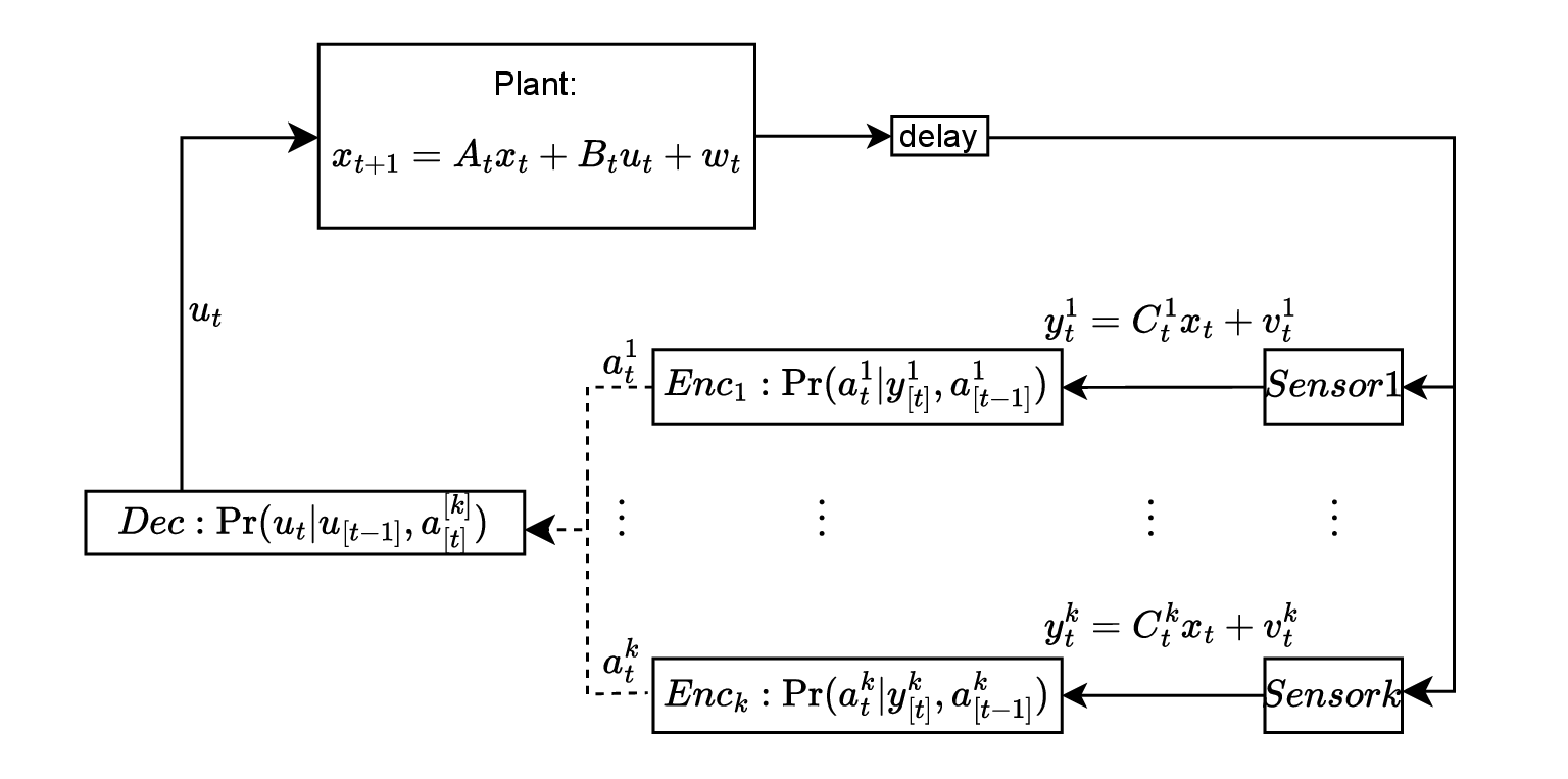
This paper considers a networked control system, as depicted in Figure 1. Specifically, the system has an LQG plant, \(k\) sensors/encoders, and one decoder. The \(k\) encoders receive signals of the plant’s output and transmit a message independently through a lossless channel with the prefix code. The decoder decodes these messages and outputs a control signal to the plant, which evolves with the plant’s output and the control signal. Two critical metrics are rates and the control cost. Rates measure the expected average bit length of the encoders’ codewords, and the control cost measures the price of control signals. The detailed definitions can be found in Section 2.

Characterizing the causal rate-distortion function is a fundamental and intriguing problem. The lower bound and the achievable schemes have been widely studied for cases with one encoder and one decoder [1]–[5], [8]–[11]. Tatikonda et al. [1] consider the scalar LQG plant with the LQR cost function and compute the causal rate distortion function. Kostina and Hassibi [3] extend the result to the vector Gaussian system with partial observation and non-Gaussian noise. [3] applies the entropy power inequality to analyze directed information and prove an analytical lower bound for the problem. [3] also shows that the causal rate distortion function for the LQG plant is essentially the same for the uncontrolled Gaussian-Markov process. The closed-form solution for the vector case is derived through the Semidefinite Programming(SDP) formulation in Tanaka et al. [2] for the LQG plant and in [8] for the Gaussian-Markov source. In [2] and [8], they first show the optimality of the linear policies for the causal rate distortion function of the LQG plant and the Gaussian-Markov source, correspondingly, and then leverage SDP to compute the optimal policies numerically.

Cuvelier and Tanaka [5] and Sabag et al. [4] consider the case with side information at the decoder. [5] considers when part of the plant state is the side information, and [4] considers the side information to be linear noisy signals. These two papers establish the optimality of linear policies and apply the SDP approach to compute the causal rate distortion function. Lev and Khina [9] consider the scalar Gaussian-Markov source with side information. For the achievable scheme, the known results are for the case without side information. Silva et al. [10] present a dithered quantization achievable scheme that is 1.254 bits away from the lower bound. Tanaka et al. [11] generalizes the achievable scheme to the vector case.

Little is known about the tradeoff between data rates and control performance in settings with multiple sensors/encoders and one decoder, as depicted in Figure 1. Stavrou et al. [12] consider optimizing the sum rate with respect to the covariance matrix and mean-square error distortions. Their formulation of the sum rate optimization is essentially the same as the point-to-point case optimization. Jung et al. [13] investigate the same scenario but with the feedback of the control signal sent from the decoder to the encoders. [13] formulates the rates-cost tradeoff as a non-convex optimization problem. However, for the networked case without feedback, the causal rate-distortion function remains an unsolved and longstanding open problem, which we aim to address in this work.

Given the optimality of linear policies for the LQG control problem with a single encoder, it is natural to hypothesize that linear policies might also be optimal in networked scenarios. This intuition is further reinforced by the optimality of linear policies in lossy source coding problems involving Gaussian sources and mean-square error distortion, such as Shannon’s lossy source coding [14], the Wyner-Ziv problem [15], quadratic Gaussian source coding [16], and the Gaussian CEO problem [17]. Yet, establishing the optimality of linear policies for networked LQG cases is highly non-trivial due to the fundamental differences between networked and point-to-point scenarios. Since the two encoders are independent in the networked case, some of the steps in establishing the optimality of linear policies for point-to-point settings would not be easily extended to the networked settings. Specifically, for the point-to-point scenario,  [2] and [4] (a) establish a directed information lower bound optimization problem for the causal rate-distortion function and (b) show that linear encoders are optimal in evaluating the lower bound. To show that linear encoders are optimal, [2] and [4] first show that Gaussian distributions are sufficient for the optimization problem, from which the optimality of linear encoders follows. In contrast, the networked case requires proving the optimality of independent linear encoders, as the encoders do not communicate. The key step of proving linear encoder optimality in [2] and [4] does not directly generalize to networked settings. This limitation necessitates the development of new lower bounds for which we can prove the optimality of independent linear encoders.

1.1 Contributions↩︎

The main contributions of this paper are as follows:

• For the networked setting, we establish a new directed information lower bound for the LQG plant, which, to the best of our knowledge, is the first lower bound derived for the multiple sensors/encoders and one decoder setting.

• For the networked setting, we demonstrate the optimality of linear, independent encoders and linear decoders for the weighted sum lower bound optimization under the full observation condition (Definition 3) for LQG plant and quadratic cost. Additionally, the original infinite-dimensional optimization problem is reduced to a finite-dimensional one, simplifying its analysis, although no convex form is obtained for the optimization problem.

• For the side information setting, our new directed information lower bound can also be used to prove that linear encoders are sufficient in the point-to-point case with linear side information. In particular, our approach provides an alternate proof for the case with side information presented in [4].

• For the side information setting, we provide SDP formulations for the causal rate distortion function for the Gaussian-Markov source with weighted mean-square error distortion and side information. Moreover, we present results for both time-variant systems and time-invariant systems with a singular noise covariance matrix, which is not included in [4].

1.2 Notations↩︎

Lowercase letters are vectors and uppercase letters are matrices. The subscripts represent time steps, and the superscripts represent the encoder index. For example, \(x_{t}\) is a vector at time step \(t\). \(y^{i}_{t}\) is the signal received by Encoder \(i\). We denote \(x_{[T]}^{\mathrm{T}} = (x_{1}^{\mathrm{T}},...,x_{T}^{\mathrm{T}})\) be the transpose of \(x_{[T]}\). Let \((x_{[T]},y_{[T]},z_{[T]})\) be a group of random variables. Define the directed information and conditional directed information as follows: \[\begin{align} I(x_{[T]}\rightarrow y_{[T]}) &=\sum_{t=1}^{T} I(x_{[t]};y_{t}|y_{[t-1]})\\ I(x_{[T]}\rightarrow y_{[T]}\Vert z_{[T]})&=\sum_{t=1}^{T} I(x_{[t]};y_{t}|y_{[t-1]},z_{[t]}) \end{align}\] Let \(S\subseteq \{1,...,k\}\) be a set of indices. We denote \(x^{S}_{t} = [x^{i}_{t}:i\in S ]\). Furthermore, the notation \((x^{S}_{[t]})^{\mathrm{T}}=[ (x^{i}_{[t]})^{\mathrm{T}}:i\in S ]\). For simplicity, we denote \([a,b] = \{a,...,b\}\) and \([t] = \{1,...,t\}\) where \(a\), \(b\) and \(t\) are integers.

1.3 Related Work↩︎

The research on the tradeoff between data rate and control performance begins with the minimum data rate required for a control system to be stabilized. A substantial body of research has been conducted on this topic, with some studies focusing on the single sensor/encoder and single decoder/controller setting, and others on the multiple sensors/encoders and multiple decoders/controllers setting. The first papers regarding the data rate and the control system are Baillieul [18] and Wong and Brockett [19]. They consider the worst-case stabilizability of the linear plant with the point-to-point lossless channel. They show that a fully observed scalar system can be bounded, i.e. \(\limsup_{t\rightarrow \infty}\Vert x_{t} \Vert < \infty\), if and only if the data rate exceeds \(\log |A|\) bits, where \(A\) is the coefficient with \(x_{t}\) in the LQG plant. Tatikonda and Mitter [20] extend the result to the vector case and show that if an LTI system is asymptotically stable, the data rate is at least \(\sum_{|\lambda_{i}(A)|>1} \log|\lambda_{i}(A)|\), where \(\lambda_{i}(A)\) are eigenvalues of \(A\). This implies that only unstable modes of the matrix \(A\) matter for stabilizability, which matches the standard intuition from the definition of stabilizability. Nair and Evans [21] consider the same setting with the mean square stabilizability, i.e. \(\limsup_{t\rightarrow \infty} \mathbb{E}\Vert x_{t} \Vert^{2}<\infty\). Schlotterbeck et al. [22] consider the communication channel with stochastic delay. Su et al. [23] and Xu et al. [24] consider the mean-square stabilizability in the presence of a fading channel.

A few papers investigate the mean-square stabilizability with multiple sensors/encoders and decoders/controllers. Zaidi et al. [25] present sufficient conditions for stabilizing two scalar LTI plants with noisy observation over the multiple access channel and the broadcast channel. Liu and Gupta [26] provide more achievable points on the rate region for the MAC channel. Zaidi et al. [27] consider two LTI plants with the interference channel. In another work [28], they present an achievable scheme, which is an adaptation of the classical Schalkwijk-Kailath scheme, developed for the transmission of reliable information over channels with noiseless feedback. In [29], Zaidi et al. examine a Gaussian relay channel and propose an achievable scheme also based on the Schalkwijk-Kailath scheme. In [30], they consider a Gaussian network relay channel, which consists of a group of relay nodes. Necessary and sufficient conditions for mean-square stabilizability over various network topologies are derived. Kumar et al. [31] consider stabilizing one LTI plant with a Gaussian product channel, in which there are multiple encoders and one decoder, and each codeword passes through an AWGN channel to the decoder. The paper provides necessary and sufficient conditions for mean-square stabilizability. In particular, the achievable scheme is nonlinear, and the condition is related to the total power allocation of the AWGN channels, noise variances, and the unstable eigenvalues.

1.4 Organization↩︎

The rest of the paper is organized as follows. In Section 2, we formulate the problem setting of the networked control system. In 3.1, we present the new directed information lower bound for the multiple sensors/encoders and one decoder setting. In 3.2, we show the optimality of linear policies for optimizing the weighted sum directed information lower bound. In 4.1, we formulate the problem for the Gaussian-Markov source. In 4.2, we apply the first two Theorems to the causal lossy compression of Gaussian-Markov sources with side information and present SDP formulations for solving the corresponding causal rate-distortion function with singular noise covariance matrices.

2 Problem Formulation↩︎

Consider the setting with \(k\) sensors/encoders and one decoder setting as depicted in Figure 1. The plant follows the following evolving process \[x_{t+1} = A_{t}x_{t}+B_{t}u_{t}+w_{t}\] where \(x_{t}\in\mathbb{R}^{n}\) are the plant states, \(u_{t}\in \mathbb{R}^{m}\) are the control signals, \(w_{t}\in\mathbb{R}^{n}\) are independent Gaussian noises following distribution \(\mathcal{N}(0,W_{t})\), \(A_{t}\in\mathbb{R}^{n\times n}\) and \(B_{t}\in\mathbb{R}^{n\times m}\). The sensor \(i\) receives a linear signal \(y^{i}_{t} = C^{i}_{t}x_{t}+v^{i}_{t}\) where \(v^{i}_{t}\) are independent Gaussian noises with distribution \(\mathcal{N}(0,V^{i}_{t})\). Note that the noises \(v^{i}_{t}\) can be correlated i.e. \(\mathbb{E}[v^{i}_{t} (v^{j}_{t})^{\mathrm{T}}]\neq 0\) or \(V^{i}_{t}\) is a singular matrix. The encoder \(i\) encodes independently from the distribution \(\Pr(a^{i}_{t}|y^{i}_{[t]},a^{i}_{[t-1]})\) and then transmits \(a^{i}_{t}\) to the decoder/controller through a lossless channel with a prefix code[32]. The decoder outputs the control signal \(u_{t}\sim\Pr(u_{t}|u_{[t-1]},a^{[k]}_{[t]})\). Let \(l(*)\) be the length of the input in terms of bits, \(\mathbb{P}\) be the measure of \((x_{[T+1]},u_{[T]})\). We are interested in characterizing the tradeoff between the expected input length and the expected control cost, which are defined as follows:

Let \(d^{*}\) be the minimal control cost such that the rates are finite. For the control cost requirement \(d\geq d^{*}\), we are interested in the following weighted sum rate optimization problem: \[\begin{align} \label{eqn:rate-distortion} \inf_{\gamma^{*} \in \Gamma^{*}, J\leq d} \limsup_{T\rightarrow \infty} \;\sum_{i=1}^{k}\lambda_{i}R_{i} \end{align}\tag{1}\] where we assume \(\lambda_{i+1}\geq \lambda_{i}\) for \(i\in [k-1]\) without loss of generality, and \(\Gamma^{*}\) is the set of measurable policies consisting of independent encoders \(\mathbb{P}(a^{[k]}_{[T]}\Vert y^{[k]}_{[T]}) \triangleq \{ \prod_{i=1}^{k}\Pr(a^{i}_{t}|y^{i}_{[t]},a^{i}_{[t-1]})\}_{t\in[T]}\), a decoder \(\mathbb{P}(u_{[T]}\Vert a^{[k]}_{[T]})\triangleq \{\Pr(u_{t}|u_{[t-1]},a^{[k]}_{[t]})\}_{t\in[T]}\).

In this paper, a lower bound on the weighted sum rate to achieve the target distortion requirement is established. We first derive the directed information lower bound for the networked control setting as in Theorem 1. We then show that linear policies are optimal for minimizing the weighted sum lower bound of 1 as in Theorem 2. As a direct application of these two derived Theorems, we establish the SDP forms to solve the causal rate-distortion function for the Gaussian-Markov source and side information with a singular noise matrix as in Theorem 4 and Theorem 5, which are not covered in [4].

3 Directed Information Lower Bound And The Optimal Linear Policy↩︎

In this section, we first derive a new lower bound on the rate \((R_{1},...,R_{k})\) required to achieve the target control cost for the networked control setting. Our bound is expressed in terms of conditional directed information. Then we show that it is sufficient to consider a linear policy set to optimize the derived weighted sum rate lower bound for \(\sum_{t=1}^{k}\lambda_{i}R_{i}\).

3.1 Directed Information Lower Bounds↩︎

For the problem illustrated in Figure 1, we establish the following directed information lower bound for the rate tuple \((R_{1},...R_{k})\) first.

For example, in the three-users case, we have the following inequalities: \[\begin{align} R_{1} &\geq I(y^{1}_{[T]} \rightarrow u_{[T]}\Vert y^{2,3}_{[T]})\\ R_{2} &\geq I(y^{2}_{[T]} \rightarrow u_{[T]}\Vert y^{1,3}_{[T]})\\ R_{3} &\geq I(y^{3}_{[T]} \rightarrow u_{[T]}\Vert y^{1,2}_{[T]})\\ R_{1} + R_{2} &\geq I(y^{1,2}_{[T]} \rightarrow u_{[T]}\Vert y^{3}_{[T]}) \\ R_{1} + R_{3} &\geq I(y^{1,3}_{[T]} \rightarrow u_{[T]}\Vert y^{2}_{[T]})\\ R_{2} + R_{3} &\geq I(y^{2,3}_{[T]} \rightarrow u_{[T]}\Vert y^{1}_{[T]})\\ R_{1} + R_{2} + R_{3} &\geq I(y^{1,2,3}_{[T]} \rightarrow u_{[T]}) \end{align}\]

Theorem 1 can be specialized to the point-to-point scenario with side information involving a single encoder, where \(y^{1}_{t} = x_{t}\) represents the signal sent to the encoder, \(y^{2}_{t} = y_{t}\) serves as the linear side information available at the decoder. Letting \(R\) denote the rate for this scenario, we can readily show the following directed information lower bound:

Theorem 1 provides the first lower bound for the networked control setting with multiple sensors/encoders and one decoder, and Corollary 1 introduces a new lower bound for the point-to-point case with side information [4], [5]. A key strength of our bounds is that we establish the optimality of linear policies for evaluating them. Specifically, we discuss the optimality of linear policies for Theorem 1 and Corollary 1 in Remark 1.

If linear encoders are optimal for the lower bounds in Theorem 1, the certainty equivalence controller, which is a linear controller with feedback control gains from the backward Riccati recursion, is optimal as in [2]. This allows one to transform the optimization problem in 2 into a finite-dimensional optimization problem. In the point-to-point settings [2], [4], [5], the optimization of the lower bound and the control cost with the certainty equivalence controller is convex. Thus, showing the optimality of linear policies is the first step. This is why we derived the lower bound in Theorem 1 even if it is suboptimal – for example, there exists a tighter lower bound, as discussed in the following Remark.

3.2 Linear Policies Are Sufficient↩︎

To characterize the lower bound we established in Theorem 1, we consider the following weighted sum lower bound for \(\sum_{i = 1}^{k}\lambda_{i}R_{i}\) in the rest of the paper: \[\begin{align} \label{eqn:weighted32sum32lower32bound} \inf_{\gamma^{*} \in \Gamma^{*}, J\leq d} &\sum_{i=1}^{k}(\lambda_{i} - \lambda_{i-1}) I(y^{[i,k]}_{[T]}\rightarrow u_{[T]} \Vert y^{[i-1]}_{[T]}) \end{align}\tag{2}\] Here the policy set \(\Gamma^{*}\triangleq \{ \Pr(u_{t}|y^{[k]}_{[t]},u_{[t-1]})\}_{t\in[T]}\) since it includes all the legit \(\{ \Pr(u_{t}|y^{[k]}_{[t]},u_{[t-1]})\}_{t\in[T]}\) induced from the policy set \(\mathbb{P}(a^{[k]}_{[T]}\Vert y^{[k]}_{[T]}) \cdot\mathbb{P}(u_{[T]}\Vert a^{[k]}_{[T]})\).

We demonstrate that a class of linear encoders and decoders is sufficient for optimization 2 under the full observation condition 3, thus reducing the original problem to a finite-dimensional optimization problem. The full observation condition is as follows:

For example, in the two encoders case, let \(x_{t} = [(x^{1}_{t})^{\mathrm{T}},(x^{2}_{t})^{\mathrm{T}}]\), \(y^{1}_{t} = x^{1}_{t}\) and \(y^{2}_{t} = x^{2}_{t}\), or \(y^{1}_{t} = x_{t}\) and \(y^{2}_{t} = x_{t} + v_{t}\). The full observation condition implies that if all the sensors sit together, they can recover the full \(x_{t}\). This condition is needed when proving an important lemma for the following Theorem:

The proof follows some steps from the paper [2]. The key idea is to show that for any policy constructed by a probability measure \(\mathbb{P}\in\Gamma^{*}\), we construct a Gaussian measure \(\mathbb{G}\) that has the same covariance matrix as \(\mathbb{P}\), and the weighted sum directed information lower bound computed by \(\mathbb{G}\) is no bigger than that computed by \(\mathbb{P}\). Next, we construct a linear policy \(\mathbb{Q}\) such that \(\mathbb{G}(y^{[k-1]}_{[t+1]},y^{k}_{t+1},u_{[t]}) = \mathbb{Q}(y^{[k-1]}_{[t+1]},y^{k}_{t+1},u_{[t]})\). Hence, the weighted sum rate lower bound is the same for policy \(\mathbb{G}\) and policy \(\mathbb{Q}\). The control cost is the same since the second moments are the same. Then, we divide the linear function of \(u_{t}\) in \(\mathbb{Q}\) into independent parts. Each part corresponds to the information available to each Encoder. This enables us to show that the optimal policy for the optimization 2 is in \(\Gamma_{1}\). Finally, we show that for any policy in \(\Gamma_{1}\), there is a policy \(\mathbb{P}\in\Gamma^{*}\) that achieves the same weighted sum rate lower bound and the same control cost. This completes the whole proof.

Throughout the proof of Theorem 2, we can show that for the point-to-point case with linear side information, optimizing the lower bound in Theorem 1 is the same as optimizing the lower bound considered in [4], as the following Proposition.

4 Causal Lossy Compression with Side Information↩︎

In this section, we consider the causal lossy compression problem of Gaussian-Markov sources with linear side information at the decoder. The causal lossy compression with the Gaussian-Markov source and the weighted mean-square error distortion is equivalent to the case with the LQG plant and the quadratic costs for the conditional directed information optimization. [3] shows this for the case without side information, and the arguments for the case with side information are similar, thus omitted here. We discuss the problem setting in Section 4.1. We show a lower bound and the optimality of linear policies in Section 4.2. We present the SDP forms for the lower bound with the time-variant system in Section 4.2.1, and with the time-invariant system in Section 4.2.2. The numerical simulations are presented in the Section 4.3.

4.1 Problem Setting↩︎

Consider the problem setting as depicted in Figure 2

with the Gaussian-Markov source given as: \[\label{eqn:csc-sid} m_{t+1} = A_{t}m_{t}+n_{t}\tag{3}\] where \(m_{t}\in\mathbb{R}^{n}\) is the state, \(n_{t}\in\mathbb{R}^{n}\) are independent Gaussian noises with covariance matrix \(N_{t}\). In this problem, there is one encoder and one decoder. The encoder observes the full \(m_{t}\) at each time step and sends the message \(a_{t}\) to the decoder with a measurable encoder \(\Pr(a_{t}|m_{[t]},a_{[t-1]})\) with the prefix code. The decoder receives \(a_{t}\) and a linear side information \(y_{t} = C_{t}m_{t} + v_{t}\), where \(C_{t}\) is a \(l\times n\) matrix and \(v_{t}\sim\mathcal{N}(0,V_{t})\) with dimension \(l\), at each time step. The optimal decoder is known to be the conditional expectation when the distortion function is the weighted mean-square error(WMSE). Let \(\hat{m}_{t}\) be the estimation of \(m_{t}\) at time step \(t\). The WMSE is defined as:

Let \(a_{t}\) be the signal sent to the receiver at time step \(t\). The measurable encoder is \(\mathbb{P}(a_{[T]}\Vert m_{[T]}) = \{\Pr(a_{t}|m_{[t]}, a_{[t-1]})\}_{t\in[T]}\) and the optimal decoder is known to be the conditional expectation \(\{\mathbb{E}[m_{t}|a_{[t]},y_{[t]}]\}_{t\in[T]}\). Let \(\Delta = \mathbb{P}(a_{[T]}\Vert m_{[T]})\cdot \mathbb{P}(\hat{m}_{[T]}\Vert a_{[T]}, y_{[T]})\) be the set of measurable encoders and decoders, \(\delta\) be any policy in \(\Delta\), and \(R^{CSC-SD} = \frac{1}{T}\mathbb{E}[l(a_{t})]\) be the average rate of codewords. We consider the following causal rate-distortion function: \[\inf_{\delta \in \Delta, \text{WMSE}\leq d} \lim_{T\rightarrow \infty} R^{CSC-SD} \label{eqn:causal-source-coding-optimization-form}\tag{5}\]

4.2 Semidefinite Programming Forms↩︎

In this subsection, we present SDP forms to compute a lower bound for the 5 . We start with a direct application of Theorem 1 and Theorem 2, showing that 5 can be lower bounded by optimizing the conditional directed information, and the optimal message is linear, as stated in the following Theorem.

The remaining part of the section applies the Semidefinite Programming(SDP) approach to explicitly compute the optimal encoder with respect to the required WMSE. The SDP formulation for the LQG plant with side information has been discussed in [4]. However, the case with the singular noise covariance matrix \(N_{t}\) is not included. In this paper, we present SDP forms with the singular noise matrix and full-rank matrices \(A_{t}\) for both time-variant and time-invariant systems. For the time-variant system, we consider a finite time step \(T\), and the objective is the directed information term with the WMSE constraint. For the time-invariant system, we consider taking the limit with respect to \(T\) and show the existence of the Ricatti recursion when \(A\) has no eigenvalues on the unit circle with the assumption that \((A,\mathrm{W})\) are detectable. We include results for the time-variant system in Section 4.2.1 and the time-invariant system in Section 4.2.2.

4.2.1 Time-Variant System↩︎

Consider a time-variant system where the system parameters are changing with respect to time, and finite \(T\). Define the lower bound optimization problem for the time-variant system as: \[\begin{align} \label{eqn:time-variant-cs} \mathrm{R}_{CS}^{TV} (d) = \inf_{\delta \in \Delta, \text{WMSE}\leq d} & I(m_{[T]}\rightarrow \hat{m}_{[T]}\Vert y_{[T]}) \end{align}\tag{6}\] Denote \(\text{Cov}\left[m|a,y\right] = \mathbb{E}[(m-\mathbb{E}[m|a,y])(m-\mathbb{E}[m|a,y])^{\mathrm{T}}]\), and define the two covariance matrices as follows: \[\begin{align} P_{t+1|t} &= \text{Cov}\left[m_{t+1}|a_{[t]},y_{[t]}\right]\\ P_{t+1|t}^{+} &= \text{Cov}\left[m_{t+1}|a_{[t]},y_{[t+1]}\right] \end{align}\] Note that \(y_{t} = C_{t}m_{t} + v_{t}\). By the standard Kalman filter equations, we have the following equalities: \[\begin{align} P_{t+1|t} &= A_{t}P_{t|t}A_{t}^{\mathrm{T}} + N_{t} \tag{7}\\ (P_{t+1|t}^{+})^{-1} &= P_{t+1|t}^{-1} + C_{t+1}^{\mathrm{T}}V_{t+1}^{-1}C_{t+1} \tag{8} \end{align}\] We have the following two SDP forms to solve the \(\mathrm{R}_{CS}^{TV}\)

4.2.2 Time-Invariant System↩︎

Consider a time-invariant system where \(A_{t} = A\), \(N_{t} = N\), \(C_{t} = C\), \(V_{t} = V\) and \(\mathrm{W}_{t} = \mathrm{W}\) for all \(t\). Note that we need to characterize the long-term average behavior of the system. We assume that \((A,\mathrm{W})\) is detectable, so that the weight matrix \(\mathrm{W}\) can capture the unstable modes of \(A\). Define the lower bound optimization problem for the time-invariant system as: \[\begin{align} \mathrm{R}_{CS}^{TI}(d) = \lim_{T\rightarrow \infty}\inf_{ \delta \in \Delta, \frac{1}{T}\text{WMSE}\leq d } & \frac{1}{T}I(m_{[T]}\rightarrow \hat{m}_{[T]}\Vert y_{[T]}) \end{align}\]

We have the following two SDP forms to solve \(\mathrm{R}_{CS}^{TI}\) as the time-invariant system.

4.3 Numerical Simulation↩︎

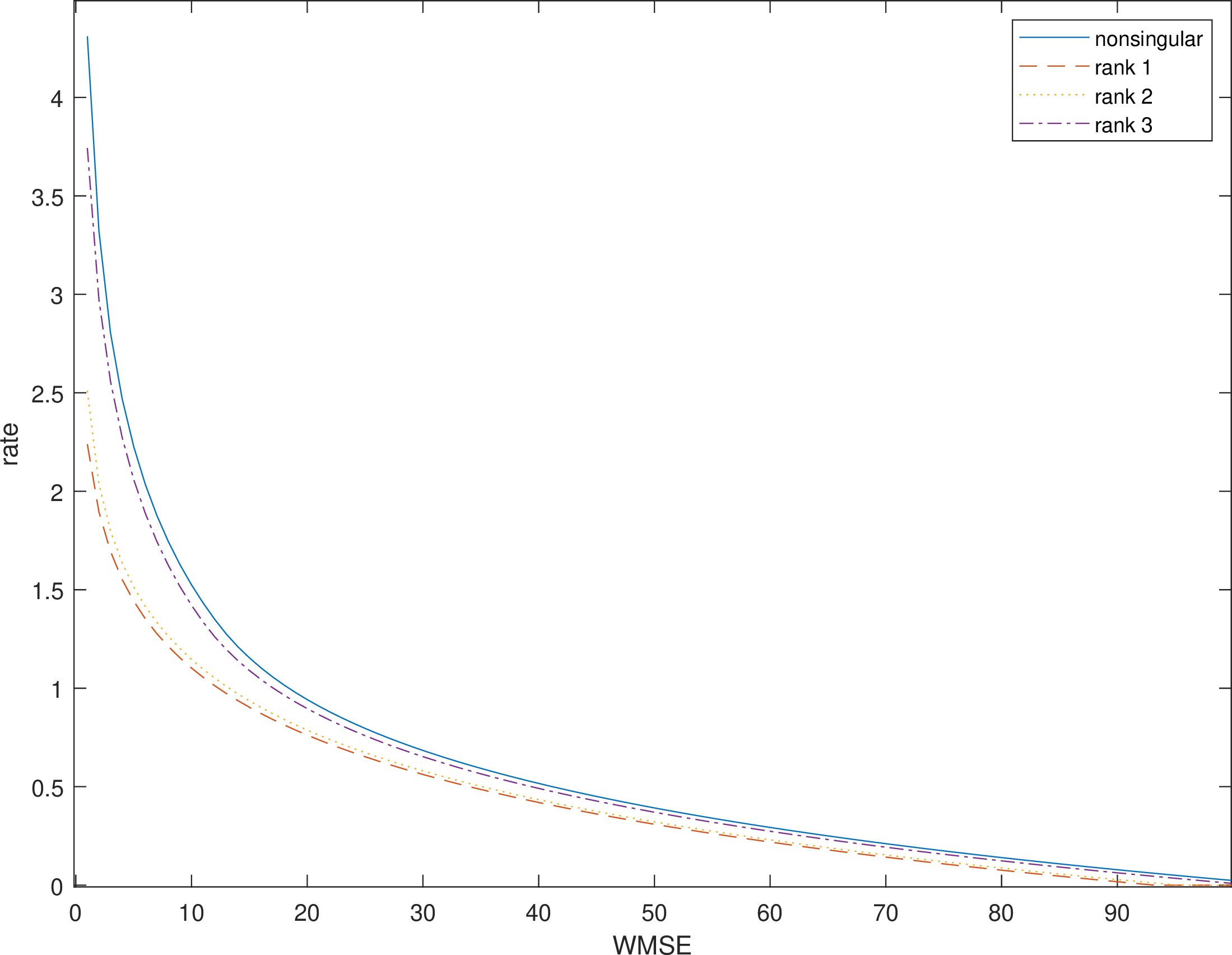
In this subsection, we present numerical simulations of the causal rate distortion function with side information for the Gaussian-Markov sources as Figure 3. We include the case when the noise covariance matrix is singular. The parameters are chosen to be the same as the side information paper [4] to compare with our new result when the noise matrix is singular. \[\begin{align} A &= \begin{bmatrix} 0.12 & 0.63 & -0.52 & 0.33\\ 0.26 & -1.28 & 1.57 & 1.13\\ -1.77 & -0.3 & 0.77 & 0.25\\ -0.16 & 0.2 & -0.58 & 0.56 \end{bmatrix}\\ N &= \begin{bmatrix} 4.94 & -0.1 & 1.29 & 0.35\\ -0.1 & 5.55 & 2.07 & 0.31\\ 1.29 & 2.07 & 2.02 & 1.43\\ 0.35 & 0.31 & 1.43 & 3.1 \end{bmatrix} \end{align}\] The weight matrix for the WMSE is chosen as the control gain computed from the Riccati equation with \(Q = I\), \(R = I\), and \[\begin{align} B &= \begin{bmatrix} 0.66 & -0.58 & 0.03 & -0.2\\ 2.61 & -0.91 & 0.87 & -0.07\\ -0.64 & -1.12 & -0.19 & 0.61\\ 0.93 & 0.58 & -1.18 & -1.21 \end{bmatrix}. \end{align}\] The side information is chosen as \(C = I\) and \(V = 10I\). We apply Cholesky decomposition to the noise matrix \(N\) and use the first \(i\) column to generate the rank \(i\) noise covariance matrix. We simulate the case where the noise covariance matrix has different ranks. The simulations imply that the higher the rank, the higher the rate.

5 Proofs↩︎

This section provides the proofs for Theorems 1, 2, 4, and 5 in Sections 5.1, 5.2, 5.3 and 5.4 respectively. Proof of Lemmas can be found in Section 5.5. Proof of the Proposition 1 is in Section 5.6.

5.1 Proof of Theorem 1↩︎

5.2 Proof of Theorem 2↩︎

Recall the policy set \(\Gamma_{1}\):

• \(c^{i}_{t} = F^{i}_{t}y^{i}_{[t]}\) for \(i \in [k-1]\);

• \(c^{k}_{t} = F^{k}_{t}y^{k}_{t} + h_{t}\) where \(h_{t}\sim \mathcal{N}(0,H_{t})\);

• \(u_{t} = \sum_{i=1}^{k}c^{i}_{t}+N_{t}u_{[t-1]}\).

Consider the policy set \(\Gamma_{2}\): \[\Gamma_{2}: u_{t} = \sum_{i=1}^{k-1}M_{t}^{i}y^{i}_{[t]} + M_{t}^{k} y^{k}_{t} + N_{t} u_{[t-1]} + g_{t} \text{, } g_{t}\sim \mathcal{N}(0,G_{t})\] To prove the Theorem 2, we aim to show the following inequalities: \[\begin{align} &\inf_{\gamma\in\Gamma^{*}:J_{\gamma}\leq D}\sum_{i=1}^{k}(\lambda_{i} - \lambda_{i-1}) I(y^{[i,k]}_{[T]}\rightarrow u_{[T]} \Vert y^{[i-1]}_{[T]}) \nonumber \\ \geq & \inf_{\gamma\in\Gamma^{*}:J_{\gamma}\leq D}\sum_{i=1}^{k}(\lambda_{i} - \lambda_{i-1})\nonumber \\&\sum_{t=1}^{T}I(y^{[i,k-1]}_{[t]},y^{k}_{t};u_{t}|u_{[t-1]},y^{[i-1]}_{[t]})\tag{10}\\ \geq& \inf_{\gamma\in \Gamma_{2}:J_{\gamma}\leq D}\sum_{i=1}^{k}(\lambda_{i} - \lambda_{i-1})\nonumber\\ &\sum_{t=1}^{T}I(y^{[i,k-1]}_{[t]},y^{k}_{t};u_{t}|u_{[t-1]},y^{[i-1]}_{[t]}) \tag{11}\\ \geq& \inf_{\gamma\in \Gamma_{1}:J_{\gamma}\leq D}\sum_{i=1}^{k}(\lambda_{i} - \lambda_{i-1})\nonumber \\ &\sum_{t=1}^{T}I(y^{[i,k-1]}_{[t]},y^{k}_{t};\sum_{j\in[i,k]}c^{j}_{t}|y^{[i-1]}_{[t]},(\sum_{j\in[i,k]}c^{j})_{[t-1]})\tag{12}\\ \geq& \inf_{\gamma\in\Gamma^{*}:J_{\gamma}\leq D}\sum_{i=1}^{k}(\lambda_{i} - \lambda_{i-1}) I(y^{[i,k]}_{[T]}\rightarrow u_{[T]} \Vert y^{[i-1]}_{[T]})\tag{13} \end{align}\]

Our goal is to first show that the policies in \(\Gamma_{2}\) give a lower bound for the optimization 2 . This shows that optimal \(u_{t}\) is a linear function of \((y^{[k-1]}_{[t]},y^{k}_{t},u_{[t-1]})\). Then, by separating the optimal \(u_{t}\) into independent parts, corresponding to each encoder, one can show that linear and independent encoders in \(\Gamma_{1}\) give a lower bound to policies in \(\Gamma_{2}\). Finally, we show that for any policy in \(\Gamma_{1}\), it is lower bounded by the original weighted sum directed information lower bound with \(\gamma\in\Gamma^{*}\) induced from the policy in \(\Gamma_{1}\). This completes our proof.

The first inequality 10 is because mutual information is non-negative. The rest of the proofs are here.

5.2.1 Proof of 11↩︎

Let \(\gamma_{P}\in \Gamma^{*}\) be a feasible policy in \(\Gamma^{*}\) and \(\gamma_{Q}\in \Gamma_{2}\) be a feasible policy in \(\Gamma_{2}\). Denote \(\mathbb{P}(y^{[k]}_{[T+1]},u_{[T]})\) be the measure generated by \(\gamma_{P}\) and similarly for \(\mathbb{Q}(y^{[k]}_{[T+1]},u_{[T]})\) be the measure generated by \(\gamma_{Q}\). We first show that \(\mathbb{P}\) is a zero-mean measure. Assume that \(\mathbb{P}\) is not zero-mean. Then, there exists another policy \(\mathrm{d}\widetilde{\mathbb{P}}(u_{t}|y^{[k]}_{[t]},u_{[t-1]}) = \mathrm{d}\mathbb{P}(u_{t}+\mathbb{E}_{\mathbb{P}}[u_{t}]|y^{[k]}_{[t]}, u_{[t-1]} )\) such that \(I_{\mathbb{P}} = I_{\widetilde{\mathbb{P}}}\) and \(J_{\widetilde{\mathbb{P}}}\leq J_{\mathbb{P}}\).

Let \(\mathbb{G}(y^{[k]}_{[T+1]},u_{[T]})\) be a Gaussian measure with the same covariance matrix as \(\mathbb{P}(y^{[k]}_{[T+1]},u_{[T]})\). The following lemma holds.

We construct \(\gamma_{Q}\in \Gamma_{2}\) by \(\mathbb{G}\). Note that \[\begin{align} \Gamma_{2}: u_{t} = \sum_{i=1}^{k-1}M_{t}^{i}y^{i}_{[t]} + M_{t}^{k} y^{k}_{t} + N_{t} u_{[t-1]} + g_{t} \text{, } g_{t}\sim \mathcal{N}(0,G_{t}) \end{align}\]

Let \(\sum_{i=1}^{k-1}M_{t}^{i}y^{i}_{[t]} + M_{t}^{k} y^{k}_{t} + N_{t} u_{[t-1]}\) be the least-mean-square-error estimation(lmsee) of \(u_{t}\) given \((y^{[k-1]}_{[t]},y^{k}_{t},u_{[t-1]})\) in \(\mathbb{G}(y^{[k]}_{[T+1]},u_{[T]})\) and let \(G_{t}\) be its error covariance matrix. Then we have \[\begin{align} &\mathrm{d}\mathbb{Q}(u_{t}|y^{[k-1]}_{[t]},y^{k}_{t},u_{[t-1]}) \nonumber\\ = &\mathcal{N}(\sum_{i=1}^{k-1}M_{t}^{i}y^{i}_{[t]} + M_{t}^{k} y^{k}_{t} + N_{t} u_{[t-1]}, G_{t}) \end{align}\]

By construction, \[\begin{align} \mathrm{d}\mathbb{G}(y^{[k-1]}_{[t]},y^{k}_{t},u_{[t]}) =& \mathrm{d}\mathbb{Q}(u_{t}|y^{[k-1]}_{[t]},y^{k}_{t},u_{[t-1]})\nonumber \\ &\cdot\mathrm{d}\mathbb{G}(y^{[k-1]}_{[t]},y^{k}_{t},u_{[t-1]}) \label{eqn:Qproperty} \end{align}\tag{14}\] Define \(\mathbb{Q}(y^{[k]}_{[T+1]},u_{[T]})\) with the given start distribution \(\mathbb{Q}(y^{[k]}_{1})\) recursively by \[\begin{align} \mathrm{d}\mathbb{Q}(y^{[k]}_{[t+1]},u_{[t]})&=\mathrm{d}\mathbb{P}(y^{[k]}_{t+1}|y^{[k]}_{t},u_{t})\mathrm{d}\mathbb{Q}(y^{[k]}_{[t]},u_{[t]})\tag{15}\\ \mathrm{d}\mathbb{Q}(y^{[k]}_{[t]},u_{[t]})&=\mathrm{d}\mathbb{Q}(u_{t}|y^{[k-1]}_{[t]},y^{k}_{t},u_{[t-1]})\mathrm{d}\mathbb{Q}(y^{[k]}_{[t]},u_{[t-1]})\tag{16} \end{align}\] where \(\mathrm{d}\mathbb{P}(y^{[k]}_{t+1}|y^{[k]}_{t},u_{t})\) is given by the plant and sensors. Then we have the following identity between \(\mathbb{Q}\) and \(\mathbb{G}\).

By the full observation condition 3, we have that \[\begin{align} J_{\gamma_{\mathbb{P}}}= J_{\gamma_{\mathbb{G}}}=J_{\gamma_{\mathbb{Q}}} \end{align}\]

This completes our proof for inequality 11 .

5.2.2 Proof of 12↩︎

Given a policy \(\gamma_{2}\in \Gamma_{2}\), we construct a policy \(\gamma_{1}\in \Gamma_{1}\) such that \(J_{\gamma_{1}} = J_{\gamma_{2}}\) and the objective functions are equal.

Let \(\gamma_{2}\in\Gamma_{2}\) given by \[u_{t} = \sum_{i=1}^{k-1}M_{t}^{i}y^{i}_{[t]} + M_{t}^{k} y^{k}_{t} + N_{t} u_{[t-1]} + g_{t}\]

Let \(c^{i}_{t} = M_{t}^{i}y^{i}_{[t]}\) for \(i\in[k-1]\) and \(c^{k}_{t} = M_{t}^{k} y^{k}_{t} + g_{t}\). So we have \(\sum_{i=1}^{t}c^{i}_{t} = u_{t} - N_{t} u_{[t-1]}\). Let \(N_{t} u_{[t-1]} = N_{t,t-1}u_{t-1} + ... + N_{t,1} u_{1}\), we have \[\sum_{i=1}^{k} \begin{bmatrix} c^{i}_{1}\\ \vdots\\ c^{i}_{t} \end{bmatrix} = \begin{bmatrix} I &\dots &0 \\ \vdots & \ddots &\vdots\\ -N_{t,1} & \dots & I \end{bmatrix} \begin{bmatrix} u_{1}\\ \vdots \\ u_{t} \end{bmatrix}\] where \(\begin{bmatrix} I &\dots &0 \\ \vdots & \ddots &\vdots\\ -N_{t,1} & \dots & I \end{bmatrix}\) is a left triangular matrix with identity matrices on the diagonal.

Hence, we have that \[\begin{align} &I(y^{[i,k-1]}_{[t]},y^{k}_{t};u_{t}|u^{t-1},y^{[i-1]}_{[t]})\\ =& I(y^{[i,k-1]}_{[t]},y^{k}_{t};\sum_{j=1}^{t}c^{j}_{t}+N_{t}u_{[t-1]}|(\sum_{j=1}^{k}c^{j})_{[t-1]},y^{[i-1]}_{[t]})\\ =& I(y^{[i,k-1]}_{[t]},y^{k}_{t};\sum_{j=i}^{t}c^{j}_{t}|(\sum_{j=i}^{k}c^{j})_{[t-1]},y^{[i-1]}_{[t]}) \end{align}\]

Since the distribution of \((y^{[k]}_{[T+1]},u_{[T]})\) is the same for \(\gamma_{1}\) and \(\gamma_{2}\), we have the same control cost. This completes our proof for inequality 12 .

5.2.3 Proof of 13↩︎

Note the \(u_{t}\) in policy set \(\Gamma_{1}\) is \(u_{t} = \sum_{i=1}^{k}c^{i}_{t}+N_{t}u_{[t-1]}\). Let \(\gamma_{1}\in\Gamma_{1}\) and construct \(\gamma\in\Gamma^{*}\) by borrowing the \(u_{t}\) of \(\gamma_{1}\), then the distribution of \((y^{[k]}_{[T+1]},u_{[T]})\) is the same for the two policies. We have the same control cost. For the objective function, we have: \[\begin{align} &I(y^{[i,k-1]}_{[t]},y^{k}_{t};\sum_{j=i}^{t}c^{j}_{t}|(\sum_{j=i}^{k}c^{j})_{[t-1]},y^{[i-1]}_{[t]})\\ = &I(y^{[i,k-1]}_{[t]},y^{k}_{t};u_{t}|u_{[t-1]},y^{[i-1]}_{[t]})\\ =&I(y^{[i,k]}_{[t]};u_{t}|u_{[t-1]},y^{[i-1]}_{[t]}) \end{align}\] The second equality is due to that \(u_{t}-(u_{[t-1]},y^{[k-1]}_{[t]},y^{k}_{t})-y^{k}_{[t-1]}\) is Markov. This completes our proof for inequality 13 .

5.3 Proof of Theorem 4↩︎

Note that \[\begin{align} \mathrm{R}_{CS}^{TV} (d) = \inf_{\delta \in \Delta, \text{WMSE}\leq d} & I(m_{[T]}\rightarrow \hat{m}_{[T]}\Vert y_{[T]}) \end{align}\] By Theorem 3, the optimal policy is in the policy set \(\Delta_{1}\). And by Proposition 1, we can rewrite \(\mathrm{R}_{CS}^{TV} (d)\) as follows: \[\begin{align} \inf_{\delta \in \Delta_{1}, \text{WMSE}\leq d}& \sum_{t=1}^{T}I(m_{t}; a_{t}|a_{[t-1]},y_{[t]}) \end{align}\]

Note that \[\begin{align} &\sum_{t=1}^{T}I(m_{t}; a_{t}|a_{[t-1]},y_{[t]})\\ =&\frac{1}{2}\log|P_{1|0}^{+}|-\frac{1}{2}\log|P_{T|T}|\\ &+\sum_{t=1}^{T-1}\frac{1}{2}\log|P_{t+1|t}^{+}| - \frac{1}{2}\log|P_{t|t}| \end{align}\]

Next, we have \[\begin{align} &\frac{1}{2}\log|P_{t+1|t}^{+}| - \frac{1}{2}\log|P_{t|t}|\\ \stackrel{(a)}{=}&-\frac{1}{2}\log|P_{t+1|t}^{-1}+C_{t+1}^{\mathrm{T}}V_{t+1}^{-1}C_{t+1}|-\frac{1}{2}\log|P_{t|t}|\\ \stackrel{(b)}{=}&\frac{1}{2}\log|V_{t+1}| - \frac{1}{2}\log|V_{t+1}+C_{t+1}P_{t+1|t}C_{t+1}^{\mathrm{T}}| \\ &+\frac{1}{2}\log|P_{t+1|t}|-\frac{1}{2}\log|P_{t|t}| \end{align}\] where \((a)\) is due to Equation 8 ; \((b)\) is due to [33].

Since \(\frac{1}{2}\log|V_{t+1}| - \frac{1}{2}\log|V_{t+1}+C_{t+1}P_{t+1|t}C_{t+1}^{\mathrm{T}}|\) is a convex function in \(P_{t|t}\), we proceed \(\frac{1}{2}\log|P_{t+1|t}|-\frac{1}{2}\log|P_{t|t}|\) next.

When \(N_{t} = L_{t}L_{t}^{\mathrm{T}}\) and \(A_{t}\) is a full rank matrix, we have \[\begin{align} &\frac{1}{2}\log|P_{t+1|t}|-\frac{1}{2}\log|P_{t|t}| \\ \stackrel{(a)}{=}& \frac{1}{2}\log|A_{t}P_{t|t}A_{t}^{\mathrm{T}}+L_{t}L_{t}^{\mathrm{T}}| - \frac{1}{2}\log|P_{t|t}|\\ \stackrel{(b)}{=}&\log|A_{t}|+\frac{1}{2}\log|P_{t|t}+A_{t}^{-1}L_{t}L_{t}^{\mathrm{T}}A^{-\mathrm{T}_{t}}|- \frac{1}{2}\log|P_{t|t}|\\ \stackrel{(c)}{=}&\log|A_{t}|+\min_{0\prec\Pi_{t}\preceq (I+L_{t}^{\mathrm{T}}A^{-\mathrm{T}}_{t}P_{t|t}^{-1}A^{-1}_{t}L_{t})^{-1}}-\frac{1}{2}\log|\Pi_{t}|\\ \stackrel{(d)}{=}&\min \log|A_{t}|-\frac{1}{2}\log|\Pi_{t}|\\ &\text{s.t. }\Pi_{t}\succ 0, \begin{bmatrix} I-\Pi_{t} & L_{t}^{\mathrm{T}}\\ L_{t} & A_{t}P_{t|t}A_{t}^{\mathrm{T}}+L_{t}L_{t}^{\mathrm{T}} \end{bmatrix}\succeq 0 \end{align}\] where \((a)\) is due to Kalman filter update Equation 7 ; \((b)\) is due to \(A_{t}\) is a full rank matrix; \((c)\) is due to that \(|I+MM^{\mathrm{T}}| = |I+M^{\mathrm{T}}M|\); \((d)\) is by matrix inversion lemma.

For constraint ?? , note we have \(P_{t+1|t+1}\preceq P_{t+1|t}^{+}\) and \((P_{t+1|t}^{+})^{-1} = P_{t+1|t}^{-1}+C_{t+1}^{\mathrm{T}}V_{t+1}^{-1}C_{t+1}\), by the matrix inversion lemma, we can write \(P_{t+1|t+1}\preceq P_{t+1|t}^{+}\) as \[\begin{align} \begin{matrix} \begin{bmatrix} P_{t+1|t}-P_{t+1|t+1} & P_{t+1|t}C_{t+1}^{\mathrm{T}}\\ C_{t+1}P_{t+1|t} & C_{t+1}P_{t+1|t}C_{t+1}^{\mathrm{T}} + V_{t+1} \end{bmatrix}\succeq 0 \end{matrix} \end{align}\]

The remaining constraints for Theorem 4 are derived from the WMSE and the Kalman filter update equation 7 .

5.4 Proof of Theorem 5↩︎

The \(\mathrm{R}_{CS}^{TI}(d)\) can be written as \[\begin{align} \inf_{\{P_{t|t}\}} &\lim_{T\rightarrow \infty}\frac{1}{T}\sum_{t=1}^{T}\frac{1}{2}(\log|AP_{t-1|t-1}A^{\mathrm{T}}+N|+\log|V|\nonumber \\ &\qquad -\log|V+C(AP_{t-1|t-1}A^{\mathrm{T}}+N)C^{\mathrm{T}}|-\log|P_{t|t}|)\tag{17}\\ \text{s.t.}&\qquad \lim_{T\rightarrow \infty} \frac{1}{T}\sum_{t=1}^{T} \text{Tr}(P_{t|t}W)\leq d \tag{18}\\ &\qquad \begin{bmatrix} P_{t|t-1} -P_{t|t} & P_{t|t-1}C^{\mathrm{T}}\\ CP_{t|t-1} & CP_{t|t-1}C^{\mathrm{T}} + V \end{bmatrix}\succeq 0 \tag{19}\\ &\qquad P_{t|t-1} = AP_{t-1|t-1}A^{\mathrm{T}} + N \end{align}\]

Define the following set \(\mathcal{D}_{0}\): \[\begin{align} \mathcal{D}_{0} = \{&P\succeq 0|\text{Tr}(P\mathrm{W})\leq d \\ &\begin{bmatrix} APA^{\mathrm{T}} + N -P & (APA^{\mathrm{T}} + N )C^{\mathrm{T}}\\ C(APA^{\mathrm{T}} + N ) & C(APA^{\mathrm{T}} + N )C^{\mathrm{T}} + V \end{bmatrix}\succeq 0 \} \end{align}\] By [34], we have that \(\mathcal{D}_{0}\) is bounded. Let \(\{P_{t|t}\}_{t\in\mathbb{N}}\) be a sequence of covariance matrices that attain the minimum in 17 . Define \(\bar{P}_{T} = \frac{1}{T}\sum_{t=1}^{T}P_{t|t}\). Following the arguments in [34], we can show that there exists a subsequence \(\{T_{i}\}_{i\in[\mathbb{N}]}\) such that \[\begin{align} \lim_{i\rightarrow \infty}\bar{P}_{T_{i}} = \bar{P}_{\infty}\in\mathcal{D}_{0}. \end{align}\]

Define \[\begin{align} f_{r,T} \triangleq& \log|A| + \frac{1}{2}\log|V| \\ &+ \frac{1}{T}\sum_{t=1}^{T} (\frac{1}{2}\log|I+L^{\mathrm{T}}A^{-\mathrm{T}}P_{t|t}^{-1}A^{-1}L|\\ &-\frac{1}{2}\log|V+C(AP_{t|t}A^{\mathrm{T}}+LL^{\mathrm{T}})C^{\mathrm{T}}|)\\ f_{s,T} \triangleq& \log|A| + \frac{1}{2}\log|V|+\frac{1}{2}\log|I+L^{\mathrm{T}}A^{-\mathrm{T}}\bar{P}_{T}^{-1}A^{-1}L| \\ &-\frac{1}{2}\log|V+C(A\bar{P}_{T}A^{\mathrm{T}}+LL^{\mathrm{T}})C^{\mathrm{T}}| \end{align}\] Since \(f_{s,T}\) is a convex function, by Jensen’s inequality we have that \[\begin{align} f_{s,T_{i}}\leq f_{r,T_{i}} \end{align}\] Let \(f_{r}\) be the objective value of 17 . We have the following lemma.

Consider the following optimization problem \[\begin{align} \inf_{P} &\frac{1}{2}(\log|\tilde{P}|+\log|V| -\log|P| \nonumber \\ &\qquad -\log|V+C\tilde{P}C^{\mathrm{T}}|)\label{eqn:TI-CS-nolimit}\\ \text{s.t.}&\qquad \text{Tr}(PW)\leq d \\ &\qquad \begin{bmatrix} \tilde{P} -P & \tilde{P}C^{\mathrm{T}}\\ C\tilde{P} & C\tilde{P}C^{\mathrm{T}} + V \end{bmatrix}\succeq 0 \\ &\qquad \tilde{P} = APA^{\mathrm{T}} + LL^{\mathrm{T}} \end{align}\tag{20}\] We have shown that there exists a feasible point in \(\mathcal{D}_{0}\) such that the objective 20 is no greater than the objective 17 . Next we show that for any feasible \(P\in \mathcal{D}_{0}\) such that the objective 20 is obtained, there exists \(\{P_{t|t}\}_{t\in[\mathbb{N}]}\) such that \(P_{t|t}\) converges to \(P\) and for this set of \(\{P_{t|t}\}_{t\in[\mathbb{N}]}\), the objective 17 is no greater than 20 .

Set \(\tilde{P} = APA^{\mathrm{T}}+N\) and \(P^{-1}-\tilde{P}^{-1} = F^{\mathrm{T}}H^{-1}F\).

Since \((A,F)\) is a detectable pair. By [35], there is a sequence of \(\{P_{t|t},P_{t|t-1}\}\) that satisfies the following recursion: \[\begin{align} P_{t|t-1} &= AP_{t-1|t-1}A^{\mathrm{T}} + N \\ P_{t|t} &= P_{t|t-1}-P_{t|t-1}F^{\mathrm{T}}(FP_{t|t-1}F^{\mathrm{T}}+H)^{-1}FP_{t|t-1} \end{align}\] with given initial \(P_{1|0}\) and converges to \((P,\tilde{P})\). For the objective 17 , we have \[\begin{align} &\lim_{t\rightarrow \infty}I(m_{t};a_{t}|a_{[t-1]},y_{t})\\ =&\lim_{t\rightarrow \infty}\frac{1}{2}\log|P_{t|t-1}^{+}| - \frac{1}{2}\log|P_{t|t}|\\ =&\lim_{t\rightarrow \infty} \frac{1}{2}(\log| P_{t|t-1}|+\log|V|\nonumber \\ &\qquad -\log|V+C P_{t|t-1}C^{\mathrm{T}}|-\log|P_{t|t}|)\\ =& \frac{1}{2}(\log|\tilde{P}|+\log|V|-\log|V+C\tilde{P}C^{\mathrm{T}}|-\log|P|)\nonumber \\ \end{align}\] And \(\lim_{t\rightarrow \infty}\text{Tr}(P_{t|t}\mathrm{W}) =\text{Tr}(P\mathrm{W}) \leq d\). Therefore, by the Cesàro mean, we have that \[\begin{align} \lim_{T\rightarrow \infty}\frac{1}{T}\sum_{t=1}^{T}I(m_{t};a_{t}|a_{[t-1]},y_{t}) &= \text{value of \eqref{eqn:TI-CS-nolimit}}\\ \lim_{T\rightarrow \infty}\frac{1}{T}\sum_{t=1}^{T}\text{Tr}(P_{t|t}\mathrm{W}) \leq d \end{align}\] This implies that the objective 17 is upper bounded by the objective 20 .

5.5 Proof of Lemmas↩︎

In this subsection, we present several useful lemmas.

5.6 Proof of Proposition 1↩︎

5.7 Proof of Lemma 1↩︎

We aim to show \[\begin{align} &\sum_{t=1}^{T}I_{\mathbb{P}}(y^{[i,k-1]}_{[t]},y^{k}_{t};u_{t}|u_{[t-1]},y^{[i-1]}_{[t]}) \\ \geq &\sum_{t=1}^{T}I_{\mathbb{G}}(y^{[i,k-1]}_{[t]},y^{k}_{t};u_{t}|u_{[t-1]},y^{[i-1]}_{[t]}) \end{align}\] Denote \(\mathrm{d}\mathbb{P} = \mathrm{d}\mathbb{P}(y^{[k]}_{[T+1]},u_{[T]})\) and \(\mathrm{d}\mathbb{G} =\mathrm{d}\mathbb{G}(y^{[k]}_{[T+1]},u_{[T]})\). Firstly, we have \[\begin{align} &\sum_{t=1}^{T} I_{\mathbb{P}}(y^{[i,k-1]}_{[t]},y^{k}_{t};u_{t}|u_{[t-1]},y^{[i-1]}_{[t]})\\ = &\sum_{t=1}^{T} \int\log(\frac{\mathrm{d}\mathbb{P}(y^{[i,k-1]}_{[t]},y^{k}_{t}|u_{[t]},y^{[i-1]}_{[t]})}{\mathrm{d}\mathbb{P}(y^{[i,k-1]}_{[t]},y^{k}_{t}|u_{[t-1]},y^{[i-1]}_{[t]})})\mathrm{d}\mathbb{P}\\ = &\sum_{t=1}^{T} \int\log( \frac{\mathrm{d}\mathbb{P}(y^{[i,k-1]}_{[t]},y^{k}_{t}|u_{[t]},y^{[i-1]}_{[t]})}{\mathrm{d}\mathbb{P}(y^{[i,k-1]}_{[t]},y^{k}_{t}|u_{[t-1]},y^{[i-1]}_{[t]}}\\ &\cdot \frac{\mathrm{d}\mathbb{P}(y^{[k]}_{t+1}|u_{[t]},y^{[k-1]}_{[t]},y^{k}_{t})}{\mathrm{d}\mathbb{P}(y^{[k]}_{t+1}|u_{[t]},y^{[k-1]}_{[t]},y^{k}_{t})})\mathrm{d}\mathbb{P}\\ =&\sum_{t=1}^{T}\int\log(\frac{\mathrm{d}\mathbb{P}(y^{[i,k-1]}_{[t+1]},y^{k}_{t+1}|u_{[t]},y^{[i-1]}_{[t+1]})}{\mathrm{d}\mathbb{P}(y^{[i,k-1]}_{[t]},y^{k}_{t}|u_{[t-1]},y^{[i-1]}_{[t]})} \\ &\cdot \frac{\mathrm{d}\mathbb{P}(y^{[i-1]}_{t+1}|u_{[t]},y^{[i-1]}_{[t]})\cdot \mathrm{d}\mathbb{P}(y^{k}_{t}|u_{[t]},y^{[k-1]}_{[t+1]},y^{k}_{t+1})}{\mathrm{d}\mathbb{P}(y^{[k]}_{t+1}|u_{[t]},y^{[k-1]}_{[t]},y^{k}_{t})})\mathrm{d}\mathbb{P}\\ = &\sum_{t=1}^{T}\int\log(\frac{\mathrm{d}\mathbb{P}(y^{[i-1]}_{t+1}|u_{[t]},y^{[i-1]}_{[t]})\mathrm{d}\mathbb{P}(y^{k}_{t}|u_{[t]},y^{[k-1]}_{[t+1]},y^{k}_{t+1})}{\mathrm{d}\mathbb{P}(y^{[k]}_{t+1}|u_{[t]},y^{[k-1]}_{[t]},y^{k}_{t})})\mathrm{d}\mathbb{P}\\ &+ \int\log(\frac{\mathrm{d}\mathbb{P}(y^{[i,k-1]]}_{T+1},y^{k}_{T+1}|u_{[T]},y^{[i-1]}_{[T+1]})}{\mathrm{d}\mathbb{P}(y^{[i,k-1]}_{1},y^{k}_{1}|y^{[i-1]}_{1})}\mathrm{d}\mathbb{P} \end{align}\] The second equality is by lemma 6 that \(\mathrm{d}\mathbb{P}(y^{[k]}_{t+1}|u_{[t]},y^{[k-1]}_{[t]},y^{k}_{t})\) is a non-degenarate Gaussian distribution, the third is by Bayes rule and rewriting the terms, and the last equality is by cancelling repeated terms.

Here, we show the proof of the first term in the last equality. The proof for the second term is similar. Consider the following:

\[\begin{align} &\sum_{t=1}^{T}\int\log(\frac{\mathrm{d}\mathbb{P}(y^{[i-1]}_{t+1}|u_{[t]},y^{[i-1]}_{[t]})\mathrm{d}\mathbb{P}(y^{k}_{t}|u_{[t]},y^{[k-1]}_{[t+1]},y^{k}_{t+1})}{\mathrm{d}\mathbb{P}(y^{[k]}_{t+1}|u_{[t]},y^{[k-1]}_{[t]},y^{k}_{t})})\mathrm{d}\mathbb{P}\\ -&\sum_{t=1}^{T}\int\log(\frac{\mathrm{d}\mathbb{G}(y^{[i-1]}_{t+1}|u_{[t]},y^{[i-1]}_{[t]})\mathrm{d}\mathbb{G}(y^{k}_{t}|u_{[t]},y^{[k-1]}_{[t+1]},y^{k}_{t+1})}{\mathrm{d}\mathbb{G}(y^{[k]}_{t+1}|u_{[t]},y^{[k-1]}_{[t]},y^{k}_{t})})\mathrm{d}\mathbb{G}\\ = &\sum_{t=1}^{T}\int\log(\frac{\mathrm{d}\mathbb{G}(y^{[k]}_{t+1}|u_{[t]},y^{[k-1]}_{[t]},y^{k}_{t})}{\mathrm{d}\mathbb{P}(y^{[k]}_{t+1}|u_{[t]},y^{[k-1]}_{[t]},y^{k}_{t})} \\ &\cdot\frac{\mathrm{d}\mathbb{P}(y^{[i-1]}_{t+1}|u_{[t]},y^{[i-1]}_{[t]})\mathrm{d}\mathbb{P}(y^{k}_{t}|u_{[t]},y^{[k-1]}_{[t+1]},y^{k}_{t+1})}{\mathrm{d}\mathbb{G}(y^{[i-1]}_{t+1}|u_{[t]},y^{[i-1]}_{[t]})\mathrm{d}\mathbb{G}(y^{k}_{t}|u_{[t]},y^{[k-1]}_{[t+1]},y^{k}_{t+1})})\mathrm{d}\mathbb{P}\\ = &\sum_{t=1}^{T}\int\log(\frac{\mathrm{d}\mathbb{P}(y^{[i-1]}_{t+1}|u_{[t]},y^{[i-1]}_{[t]})\mathrm{d}\mathbb{P}(y^{k}_{t}|u_{[t]},y^{[k-1]}_{[t+1]},y^{k}_{t+1})}{\mathrm{d}\mathbb{G}(y^{[i-1]}_{t+1}|u_{[t]},y^{[i-1]}_{[t]})\mathrm{d}\mathbb{G}(y^{k}_{t}|u_{[t]},y^{[k-1]}_{[t+1]},y^{k}_{t+1})})\mathrm{d}\mathbb{P}\\ \geq &0 \end{align}\] The first equality is by \(\mathbb{P}\) and \(\mathbb{G}\) having the same covariance matrix, and \(\mathbb{G}\) is a Gaussian measure. The second equality is by Lemma 6. The last inequality is due to the non-negativity of the KL divergence. This completes our proof for Lemma 1.

5.8 Proof of Lemma 2↩︎

We prove by induction. For the base case, \(\mathbb{G} (y^{[k]}_{1}) = \mathbb{Q} (y^{[k]}_{1})\) by input Gaussian distribution. We assume that for time step \(t-1\), the identity holds. Then we show for time step \(t\):

\[\begin{align} &\mathbb{Q}(y^{[k-1]}_{[t+1]},y^{k}_{t+1},u_{[t]}) \\ =& \int_{y^{k}_{t}}\mathrm{d}\mathbb{Q}(y^{[k-1]}_{[t+1]},y^{k}_{t+1},u_{[t]},y^{k}_{t})\\ \stackrel{(a)}{=}& \int_{y^{k}_{t}}\mathrm{d}\mathbb{P}(y^{[k]}_{t+1}|y^{[k]}_{t},u_{t}) \mathrm{d}\mathbb{Q}(y^{k}_{t},y^{[k-1]}_{[t]},u_{[t]})\\ =& \int_{y^{k}_{t}}\mathrm{d}\mathbb{P}(y^{[k]}_{t+1}|y^{[k]}_{t},u_{t}) \mathrm{d}\mathbb{Q}(u_{t}|y^{[k-1]}_{[t]},y^{k}_{t},u_{[t-1]})\nonumber\\ &\mathrm{d}\mathbb{Q}(y^{[k-1]}_{[t]},y^{k}_{t},u_{[t-1]})\\ \stackrel{(b)}{=}&\int_{y^{k}_{t}}\mathrm{d}\mathbb{P}(y^{[k]}_{t+1}|y^{[k]}_{t},u_{t}) \mathrm{d}\mathbb{Q}(u_{t}|y^{[k-1]}_{[t]},y^{k}_{t},u_{[t-1]})\nonumber\\ &\mathrm{d}\mathbb{G}(y^{[k-1]}_{[t]},y^{k}_{t},u_{[t-1]})\\ \stackrel{(c)}{=}&\int_{y^{k}_{t}}\mathrm{d}\mathbb{P}(y^{[k]}_{t+1}|y^{[k]}_{t},u_{t}) \mathrm{d}\mathbb{G}(y^{[k-1]}_{[t]},y^{k}_{t},u_{[t]})\\ =&\int_{y^{k}_{t}} \mathrm{d}\mathbb{G}(y^{[k-1]}_{[t+1]},y^{k}_{t+1},u_{[t]},y^{k}_{t})\\ =&\mathbb{G}(y^{[k-1]}_{[t+1]},y^{k}_{t+1},u_{[t]}) \end{align}\]

where (a) is by Lemma 6, (b) applies the hypothesis assumption, and (c) applies equation 14 . This completes our proof for Lemma 2.

5.9 Proof of Lemma 4↩︎

5.10 Proof of Lemma 3↩︎

6 Conclusion↩︎

We studied the tradeoff between the communication rate and the control cost in the multiple sensors/encoders and one decoder setting. We established a new directed information lower bound and proved that linear policies are optimal for optimizing the weighted sum rate lower bound. We applied the results to the causal lossy compression of Gaussian-Markov sources with linear side information and present SDP formulations to solve the causal rate distortion function with a singular noise covariance matrix. For future research direction, one direction is to try to show the optimality of the linear policy for the tighter directed information lower bound as stated in Remark 2.

References↩︎

---

1. Funding ackowledgement↩︎

2. Sijie Li and Hyeji Kim are with the University of Texas at Austin, Austin, TX 78712 USA (email: sijieli@utexas.edu; hyeji@utexas.edu).↩︎

3. Takashi Tanaka is with the Purdue University, West Lafayette, IN 47907 USA (e-mail: tanaka16@purdue.edu).↩︎