MDL Meets Latent Confounders: LNML-based Causal Discovery
July 05, 2026
Abstract
Causal discovery with nonlinear mechanisms and latent confounders remains challenging. Existing methods often rely on either linear assumptions or causal sufficiency, limiting their applicability. We propose an MDL-based causal discovery framework that explicitly accounts for latent confounders while allowing flexible nonlinear mechanisms by minimizing the luckiness normalized maximum likelihood (LNML) code-length. The causal relationship between each variable pair is determined by selecting the shortest code-length of the causal model, and we introduce the notion of \(\Delta\)-pseudo-collinearity to identify dependencies induced by latent confounders. Based on these ideas, we develop a greedy algorithm, termed Pseudo-Collinearity Guided Causal Discovery (PCG-CD). Experiments on synthetic and real-world datasets demonstrate that the proposed method accurately recovers directed causal relationships and effectively detects latent confounders.
1 Introduction↩︎
1.1 Motivation↩︎
Understanding causation is a fundamental problem in science, as it enables the identification of underlying relationships among variables in complex systems.
Most existing causal discovery methods assume causal sufficiency, meaning that all relevant variables are observed and no latent confounders exist. However, confounding factors are ubiquitous in real-world systems and pose major challenges for causal estimation. When analyzing the relationship between two variables \(X\) and \(Y\), the observed dependence may arise from a direct causal effect, or from a latent confounder \(Z\) acting as a common cause. Only a limited number of approaches relax the causal sufficiency assumption, yet failing to account for confounders can introduce substantial bias and lead to incorrect conclusions.
In addition, causal mechanisms in practical applications, such as biology, neuroscience, economics, and climate science, are rarely linear. Restricting models to linear relationships risks model misspecification and may further obscure causal structure, particularly in the presence of latent factors. Incorporating nonlinear mechanisms is therefore essential for improving identifiability and robustness in causal discovery.
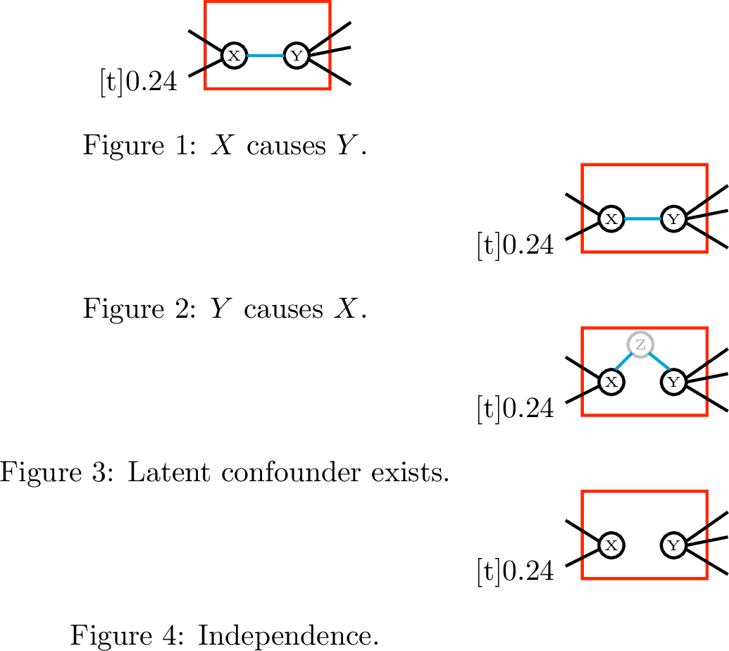
Kaltenpoth and Vreeken [1] suggested that an information-theoretic approach can help mitigate overfitting when estimating causal models with confounders. For example, suppose \(X \not\perp\!\!\!\perp Y\) is observed. If \(X\) causes \(Y\) and no confounder is present, the joint distribution follows \(P(X,Y) = P(X)P(Y|X)\). Alternatively, if a confounder \(Z\) influences both \(X\) and \(Y\), the joint distribution becomes \(P(X,Y,Z) = P(Z)P(X|Z)P(Y|Z)\). A straightforward method to identify a confounder is to check whether we can construct \(\hat{Z}\) such that \(X \perp\!\!\!\perp Y \mid Z\). A trivial solution is to set \(\hat{Z} = X\), which ensures conditional independence even in the absence of a true confounder. Therefore, it is necessary to consider both the complexity of \(\hat{Z}\) and its effect on \(X\) and \(Y\).
Motivated by this observation, we adopt the minimum description length (MDL) principle [2]–[4] for causal discovery. Under this framework, the causal relationship between any two variables, whether \(X \rightarrow Y\), \(X \leftarrow Y\), \(X \leftarrow Z \rightarrow Y\), or independence, is determined by selecting the model with the shortest code-length, as illustrated in Figure 1. We employ the luckiness normalized maximum likelihood (LNML) code-length [3], [5], which avoids explicit parameter priors and naturally incorporates sparsity through the luckiness function.
In this work, we address causal discovery with latent confounders by estimating nonlinear causal models through LNML-based model selection under the MDL principle.
1.2 Related Work↩︎
Classical causal discovery methods include constraint-based and score-based approaches. Constraint-based methods such as PC [6] infer a causal graph by testing conditional independencies and applying orientation rules, while FCI extends PC to allow latent confounders. Score-based methods, such as GES [7] and its variants [8], employ greedy search with penalized likelihood criteria but may converge to local optima.
To achieve identifiability beyond Markov Equivalence Classes (MECs), functional causal models (FCMs) impose assumptions on structural equations and noise distributions, including LiNGAM [9] with linear non-Gaussian mechanisms and ANM [10] with nonlinear relationships. Within the LiNGAM framework, ICA-LiNGAM [9] and DirectLiNGAM [11] recover full causal orderings under causal sufficiency, while ParceLiNGAM [12] and RCD [13] address unmeasured confounding by identifying variable pairs influenced by latent common causes and producing partially directed graphs with bidirected edges. Other extensions consider post-nonlinear assumptions [14] or address latent confounding in restricted settings, including CoCa [1] for nonlinear pairwise relations, CLOUD [15] for discrete data, and NOCADILAC [16], which models latent factors under a post-nonlinear assumption.
Information-theoretic approaches formulate causal discovery as a model selection problem under the MDL principle. Early methods such as SLOPE [17] and ORIGO [18] focus on bivariate or local causal direction, while GLOBE [19] extends MDL-based scoring to multivariate graphs under causal sufficiency. To relax the causal sufficiency assumption, latent-variable extensions based on MDL have been explored in model selection and causal discovery. For example, the decomposed normalized maximum likelihood (DNML) code-length criterion was proposed for hierarchical latent variable models [20], while methods such as CDHC [21] introduce hidden variables when doing so reduces the overall description length, though existing results mainly focus on linear Gaussian mechanisms.
Unlike existing MDL-based approaches that primarily assume linear Gaussian mechanisms or focus on limited settings, our method performs multivariate causal graph discovery with latent confounders under nonlinear mechanisms in continuous data, using LNML code-lengths for principled model selection.
1.3 Significance and Novelty↩︎
LNML-based code-length for causal models with latent confounders. We introduce an LNML-based code-length formulation for estimating causal graphs in the presence of latent confounders. By adopting a tractable approximation under mild assumptions on the causal equations, the proposed framework enables efficient model selection without restricting the form of the causal mechanisms. To the best of our knowledge, this is the first MDL-based method that estimates causal graphs with latent confounders in a mechanism-agnostic manner.
Identification of latent confounders via pseudo-collinearity. We propose the notion of \(\Delta\)-pseudo-collinearity to identify latent confounders through differences in code-length. We establish a theoretical result showing that this gap grows at most linearly with the sample size in linear settings, with the coefficient determined by the noise level and the similarity of the causal mechanisms. We also discuss extensions to nonlinear cases.
PCG-CD: an efficient causal discovery algorithm. We develop the PCG-CD algorithm, a greedy causal discovery algorithm that explicitly handles latent confounders. Compared to GES and related score-based methods with \(O(|V|^3)\) complexity, PCG-CD reduces edge evaluation to \(O(|V|^2)\).
Empirical validation. Extensive experiments on both synthetic and real-world datasets demonstrate that PCG-CD accurately recovers directed causal relationships and effectively detects latent confounders.
Code and supplementary material are available at: https://github.com/ZYQue/PCG-CD.
2 Notation and Preliminaries↩︎
We introduce the notation and assumptions for causal models, first under causal sufficiency and then extending to settings with latent confounders. We also summarize the MDL-based code-length formulation used throughout the paper.
2.1 Causal Model↩︎
We begin with a setting with causal sufficiency. A causal model is defined as \(M=(G,F)\), where \(G=(\boldsymbol{V},\boldsymbol{E})\) is a directed acyclic graph (DAG) over continuous variables \(\boldsymbol{V}=\boldsymbol{X}\in\mathbb{R}^d\), and \(F=\{f_i\}_{i=1}^d\) denotes the causal mechanisms. An edge \(X_{(i)}\to X_{(j)}\) indicates that \(X_{(i)}\) is a parent of \(X_{(j)}\).
The causal relationships between variables are described by structural equation models (SEMs) [22]: \[\nonumber X_{(i)} = f_i(\text{pa}_i) + \varepsilon_i, \quad \varepsilon_i \perp\!\!\!\perp \text{pa}_i,\] where \(\text{pa}_i\) denotes the parents of \(X_{(i)}\) in \(G\), \(f_i\) is the causal function, and \(\varepsilon_i\) represents noise.
We then relax causal sufficiency by allowing latent confounders. Let \(\boldsymbol{Z}\) denote unobserved variables that may jointly influence observed variables. The DAG including the confounders is then represented as \(G = (\boldsymbol{V}, \boldsymbol{E})\), where \(\boldsymbol{V} = (\boldsymbol{X}, \boldsymbol{Z})\). The causal relationship for variable \(X_{(i)}\) becomes: \[\nonumber X_{(i)} = f_i(\text{pa}_i, \text{pa}_i^Z) + \varepsilon_i, \quad \varepsilon_i \perp\!\!\!\perp (\text{pa}_i, \text{pa}_i^Z),\] where \(\text{pa}_i\) denotes the set of observed parents of \(X^{(i)}\) in \(G\), and \(\text{pa}_i^Z\) denotes the set of latent parents of \(X^{(i)}\).
2.2 Minimum Description Length Principle↩︎
According to the MDL principle, the optimal model is the one with the minimum normalized maximum likelihood (NML) code-length [23]. In this work, we adopt the luckiness normalized maximum likelihood (LNML) code-length [3] for causal model selection. LNML extends the original NML formulation by incorporating prior knowledge through a penalty term. This allows us to enforce sparsity in the causal DAG and to control the complexity of the causal mechanisms. In our framework, the LNML code-length is computed from the normalized maximum posterior distribution, incorporating a sparsity constraint.
The LNML distribution is defined over a model class \(\mathcal{M}\), where \(p(\boldsymbol{X};M)\) denotes the probability density of data \(X\) under model \(M\), and \(g(M)\) is a penalty function that controls model complexity. It is given by \[p_{\text{LNML}} (\boldsymbol{X}) := \frac{\max_{M \in \;\mathcal{M}} p(\boldsymbol{X};M) e^{-g(M)}}{C_n}, \label{eq:LNML95prim}\tag{1}\] where \[C_n := \int \max_{M \in \mathcal{M}} p(\boldsymbol{X};M) e^{-g(M)} d \boldsymbol{X}, \nonumber\] also referred to as the parametric complexity, is evaluated over all possible data \(\boldsymbol{X}\) of length \(n\).
The LNML code-length is defined as the negative log-likelihood of 1 : \[\begin{align} \mathcal{L}_{\text{LNML}}(\boldsymbol{X}) &= -\log p_{\text{LNML}}(\boldsymbol{X}) \nonumber\\ &= \underset{M \in \mathcal{M}}{\min} \{ -\log p(\boldsymbol{X};M) + g(M) \} + \log C_n. \label{eq:LNML95codelength} \end{align}\tag{2}\] When the penalty term \(g(\cdot)\) is omitted, 2 reduces to the original NML code-length. Computing the LNML code-length is intractable due to the parametric complexity term \(C_n\), so an approximation is used. To preserve MDL properties, the approximation is constructed as an upper bound on \(C_n\), whose form depends on the probability model \(p(\cdot)\), the penalty function \(g(\cdot)\), and the data assumptions.
3 Luckiness Normalized Maximum Likelihood Code-length for Causal Model Discovery↩︎
To flexibly model nonlinear causal mechanisms and enable principled model selection in the presence of latent confounders, we assume Gaussian process models and develop an LNML-based code-length for scoring causal models.
3.1 Assumptions on the Causal Mechanism↩︎
We model causal mechanisms using Gaussian processes (GPs) [24]. A GP is a collection of random variables such that any finite subset follows a multivariate normal distribution, and the associated function satisfies \[f(x) \sim \mathcal{GP}(m(x), \kappa(x,x')),\] where \(m(x)=\mathbb{E}[f(x)]\) is the mean function, with the expectation taken with respect to the Gaussian process prior over functions, and \(\kappa(x,x')\) is the covariance (kernel) function.
Assuming GP mechanisms removes the restrictive linearity assumption between a variable and its parents. A GP can also be represented as a linear model in a (possibly infinite-dimensional) feature space: \(f=\sum_i \alpha_i \phi_i\).
Given data \(\{(x_i,y_i)\}_{i=1}^n\), we assume \[y_i = f(x_i) + \varepsilon_i,\quad \varepsilon_i \sim \mathcal{N}(0,\sigma^2),\] so that the outputs \(\boldsymbol{y}\) follow a joint Gaussian distribution: \[\boldsymbol{y} \sim \mathcal{N}(\boldsymbol{m}, \boldsymbol{K} + \sigma^2 \boldsymbol{I}),\] where \(\boldsymbol{m}=[m(x_1),\ldots,m(x_n)]^T\) and \(\boldsymbol{K}_{ij}=\kappa(x_i,x_j)\).
For a given \(x\), the mechanism can be estimated as: \[\begin{align} f(x) &= [\kappa(x_1,x),\ldots,\kappa(x_n,x)]^T(\boldsymbol{K}+\sigma^2\boldsymbol{I})^{-1}\boldsymbol{y} \nonumber\\ &= \sum_{i=1}^n \alpha_i \kappa(x_i,x), \label{eq:f40x41} \end{align}\tag{3}\] where \(\boldsymbol{\alpha}=(\boldsymbol{K}+\sigma^2\boldsymbol{I})^{-1}\boldsymbol{y}\) and \(\alpha_i\) is the \(i\)th value of this vector.
GPs are adopted for two reasons. First, the induced reproducing kernel Hilbert space (RKHS) \(\mathcal{H}\) may be infinite-dimensional, enabling a nonparametric representation of causal mechanisms and their code-lengths. Second, as shown by Kakade et al. [25], GP-based learning minimizes penalized regret, which aligns with the minimax formulation underlying NML code-length [23]. Note that not all model classes admit a valid NML distribution.
We use the radial basis function (RBF) kernel \[\kappa(x,x') = \sigma_f^2 \exp\!\left(-\tfrac{1}{2l}\|x-x'\|_2^2\right), \label{eq:kernel}\tag{4}\] as it is widely used in practice.
3.2 Luckiness Normalized Maximum Likelihood Code-length↩︎
We first define the MDL score without confounders based on Gaussian process (GP) mechanisms. For a target variable \(X_{(i)}\) with parents \(\text{pa}_i(G)\) in a causal graph \(G\), we fit a GP regression \(f_i:\text{pa}_i(G)\to X_{(i)}\). Let \(p(X_{(i)}|\text{pa}_i(G))\) denote the conditional probability of \(X_{(i)}\) given its parent variables \(\text{pa}_i(G)\), as induced by the Gaussian process regression model. The corresponding Bayesian score is given by [25], [26] \[\begin{align} L(X_{(i)}|\text{pa}_i(G)) := & \underset{f_i \in \mathcal{H}_\kappa}{\min} \big( -\log p(X_{(i)} | \text{pa}_i(G)) \nonumber\\ & \qquad\qquad + \|f_i\|_\kappa^2 \big)+ \tfrac{1}{2} \log \det \left( \sigma^{-2} \boldsymbol{K}_{\text{pa}_i(G)} + \boldsymbol{I} \right),\label{eq:mdl95score} \end{align}\tag{5}\] where \(\|f_i\|_\kappa^2\) penalizes the complexity of the mechanism. For GP models learned from finite data, this term can be computed as \[\|f_i\|_\kappa^2 = \boldsymbol{\alpha}^T \boldsymbol{K}_{\text{pa}_i(G)} \boldsymbol{\alpha},\] with kernel matrix \(\boldsymbol{K}_{\text{pa}_i(G)}\) constructed using the kernel function defined in 4 and vector \(\boldsymbol{\alpha}\) defined in 3 .
The score in 5 can be viewed as an upper bound on the negative log-likelihood under a Bayesian prior, assuming the model follows a Gaussian process [26]. As shown by Kakade et al. [25], this Bayesian prior distribution and the penalized NML density correspond to the same underlying distribution, where \(\|f_i\|_\kappa^2\) acts as a luckiness function in the LNML framework [3].
The overall description length of a causal graph \(G\) is defined as \[\begin{align} \nonumber L(\boldsymbol{X}|G) := \sum_{i=1}^d L(X_{(i)}|\text{pa}_i(G)), \end{align}\] and the optimal causal model \(\hat{M}=(\hat{G},\hat{F})\), where \(\hat{G}\) denotes the estimated causal graph and \(\hat{F}\) denotes the corresponding estimated causal mechanisms, is obtained by first solving \[\hat{G}=\arg\min_G L(X|G), \nonumber\] after which \(\hat{F}\) is estimated by Gaussian process regression.
We now extend this formulation to settings with latent confounders. Consider two variables \(X\) and \(Y\) and a confounder \(Z\). Given a causal graph \(G\) with known relationships, we can infer the unknown relationship between \(X\) and \(Y\) by comparing the description lengths of four candidate models: \[X\to Y,\quad Y\to X,\quad X\leftarrow Z\rightarrow Y,\quad X\nleftrightarrow Y .\] The MDL score for this reduced system is \[\begin{align} L(X,Y|\text{pa}_X,\text{pa}_Y,Z) := \min \bigl\{ &L(X \rightarrow Y), L(Y \rightarrow X),\nonumber\\ &L(X \leftarrow Z \rightarrow Y), L(X\nleftrightarrow Y) \bigr\}, \label{eq:mdl95XYZ} \end{align}\tag{6}\] where \[\begin{align} &L(X \rightarrow Y) := L(Y|\text{pa}_Y,X) + L(X|\text{pa}_X), \nonumber\\ &L(Y \rightarrow X) := L(X|\text{pa}_X,Y) + L(Y|\text{pa}_Y), \nonumber \\ &L(X \leftarrow Z \rightarrow Y) := L(X|\text{pa}_X,Z) + L(Y|\text{pa}_Y,Z), \nonumber \\ &L(X\nleftrightarrow Y) := L(X|\text{pa}_X) + L(Y|\text{pa}_Y). \label{eq:4types95origin} \end{align}\tag{7}\] Since the MDL score in 5 penalizes the complexity of \(f\), setting \(\hat{Z} = X\) would maximize the likelihood but would fail to minimize the description length. This approach avoids the overfitting issue discussed by Kaltenpoth and Vreeken [1].
Finally, for a causal model \(M=(G,F)\) with observed variables and latent confounders, the resulting computable LNML objective is \[\begin{align} \bar{\mathcal{L}}_{\text{LNML}}(\boldsymbol{X}) := & \sum_{i=1}^d \biggl\{ -\log p(X_{(i)}|\text{pa}_i(G)) \nonumber \\ & \qquad \qquad \qquad + \|f_i\|_\kappa^2 + \tfrac{1}{2} \log \det \left( \sigma^{-2} \boldsymbol{K}_{\text{pa}_i(G)} + \boldsymbol{I} \right) \biggr\}. \label{eq:computable95LNML} \end{align}\tag{8}\] The optimal graph is obtained by minimizing \(\bar{\mathcal{L}}_{\text{LNML}}(\boldsymbol{X}|G)\) over \(G\).
4 Algorithm for Solving a Causal Model with Latent Confounders↩︎
While LNML code-length can be defined with latent confounders, its direct computation is challenging due to reliance on sampling over unobservable variables. To address this issue, we introduce a computable approximation of the latent-confounder-aware code-length that removes sampling dependence. Based on this approximation, we propose the notion of pseudo-collinearity to theoretically characterize and identify latent confounding. These ideas lead to a novel causal discovery algorithm, Pseudo-Collinearity Guided Causal Discovery (PCG-CD), which departs from conventional score-based methods by explicitly incorporating latent confounder detection into model selection.
4.1 Reformulation of Code-length↩︎
In this work, we assume the presence of latent confounders, under which statistical dependencies may need to be jointly explained by observable variables and unobservable variables (latent confounders). To simplify the exposition, we henceforth focus on the residual components of variables when considering a pair of nodes \(A\) and \(B\).
The residual component of a node is defined as the original variable minus the part explained by its known parents in the causal graph \(G\). We denote the residual component of \(A\) by \(A_{\text{res}}\). Under this formulation, the causal relationship between \(A\) and \(B\) can be identified by examining \(A_{\text{res}}\) and \(B_{\text{res}}\), without reference to other observed nodes in \(G\).
Under this setting, we consider a reduced system consisting of \(A_{\text{res}}\), \(B_{\text{res}}\), and an unobserved variable \(Z\). The four candidate models differ only in the assumed causal structure among these variables, while \(Z\) is treated as present in all candidate models. The corresponding code-lengths 7 can be rewritten as follows: \[\begin{align} & L(A_{\text{res}}|\text{pa}_{A_{\text{res}}}=\emptyset)+L(B_{\text{res}}|\text{pa}_{B_{\text{res}}}=A_{\text{res}}) + L(Z),\nonumber\\ & L(A_{\text{res}}|\text{pa}_{A_{\text{res}}}=B_{\text{res}})+L(B_{\text{res}}|\text{pa}_{B_{\text{res}}}=\emptyset) + L(Z), \nonumber\\ & L(A_{\text{res}}|\text{pa}_{A_{\text{res}}}=Z)+L(B_{\text{res}}|\text{pa}_{B_{\text{res}}}=Z) + L(Z),\nonumber\\ &L(A_{\text{res}}|\text{pa}_{A_{\text{res}}}=\emptyset)+L(B_{\text{res}}|\text{pa}_{B_{\text{res}}}=\emptyset) + L(Z). \nonumber \end{align}\] Since \(L(Z)\) can be treated as constant, we can ignore it when comparing the code-lengths of the four cases.
We can also reformulate the code-lengths of the four cases as follows: \[\begin{align} &L(A_{\text{res}} \rightarrow B_{\text{res}}) = L(A_{\text{res}}|\text{pa}_{A_{\text{res}}}=\emptyset)+L(B_{\text{res}}|\text{pa}_{B_{\text{res}}}=A_{\text{res}}) ,\nonumber\\ &L(A_{\text{res}} \leftarrow B_{\text{res}}) = L(A_{\text{res}}|\text{pa}_{A_{\text{res}}}=B_{\text{res}})+L(B_{\text{res}}|\text{pa}_{B_{\text{res}}}=\emptyset) ,\nonumber\\ &L(A_{\text{res}} \leftrightarrow B_{\text{res}}) = L(A_{\text{res}}|\text{pa}_{A_{\text{res}}}=B_{\text{res}})+L(B_{\text{res}}|\text{pa}_{B_{\text{res}}}=A_{\text{res}}) ,\nonumber\\ &L(A_{\text{res}} \nleftrightarrow B_{\text{res}}) = L(A_{\text{res}}|\text{pa}_{A_{\text{res}}}=\emptyset)+L(B_{\text{res}}|\text{pa}_{B_{\text{res}}}=\emptyset) \nonumber, \end{align}\]where \(A_{\text{res}} \leftrightarrow B_{\text{res}}\) denotes the case where a latent confounder causes both \(A\) and \(B\), and \(A_{\text{res}} \nleftrightarrow B_{\text{res}}\) denotes the case where no causal relationship exists between \(A\) and \(B\). The code-length of the case with latent confounder \(L(A_{\text{res}} \leftrightarrow B_{\text{res}})\) serves as an approximation to \(L(A_{\text{res}}|\text{pa}_{A_{\text{res}}}=Z)+L(B_{\text{res}}|\text{pa}_{B_{\text{res}}}=Z)\) by replacing \(Z\) with \(A_{\text{res}}\) and \(B_{\text{res}}\). This approximation is heuristic in nature. Intuitively, one may expect \(L(A_{\text{res}}|\text{pa}_{A_{\text{res}}}=B_{\text{res}})\) to approach \(L(A_{\text{res}}|\text{pa}_{A_{\text{res}}}=Z)\) when \(B = f(Z) + \varepsilon_B\), provided that the function \(f(\cdot)\) is simple and the noise term \(\varepsilon_B\) is small (e.g., \(B = Z + \mathcal{N}(0, 0.0001)\)).
Since the quality of this approximation may vary with the complexity of the causal mechanisms, we do not use it to determine causal relationship types under the MDL principle. Instead, it is introduced solely to make the overall code-length of causal graphs with latent confounders computable, eliminating the need for explicit sampling of latent confounder values. This intuition extends naturally to the original nodes \(A\) and \(B\) in the causal graph \(G\).
4.2 Pseudo-collinearity↩︎
After accounting for observable influences, if residuals of two nodes remain similarly dependent in both directions, we infer a shared latent confounder. We call this property pseudo-collinearity.
Pseudo-collinearity holds if: \[\begin{align} & L(A_{\text{res}}|\text{pa}_{A_{\text{res}}}=B_{\text{res}})+L(B_{\text{res}}|\text{pa}_{B_{\text{res}}}=\emptyset)\nonumber\\ & \qquad \qquad \approx L(A_{\text{res}}|\text{pa}_{A_{\text{res}}}=\emptyset)+L(B_{\text{res}}|\text{pa}_{B_{\text{res}}}=A_{\text{res}}). \label{eq:pcl} \end{align}\tag{9}\] If the difference between the left-hand side and right-hand side of 9 is large, meaning that the code-length of either \(A \rightarrow B\) or \(A \leftarrow B\) is significantly smaller, then the causal relationship between \(A\) and \(B\) is unidirectional and no latent factor is present. More specifically, we say that a pair of variables \(A\) and \(B\) exhibits \(\Delta\)-pseudo-collinearity if \[\begin{align} \Delta &= |L(A_{\text{res}}|\text{pa}_{A_{\text{res}}}=\emptyset)+L(B_{\text{res}}|\text{pa}_{B_{\text{res}}}=A_{\text{res}})\label{eq:dpcl} \\ & \qquad \qquad - \Big( L(A_{\text{res}}|\text{pa}_{A_{\text{res}}}=B_{\text{res}})+L(B_{\text{res}}|\text{pa}_{B_{\text{res}}}=\emptyset) \Big)| \leq n\epsilon, \nonumber \end{align}\tag{10}\] where \(n\) denotes the sample size and \(\epsilon\) is a predefined threshold. \(\Delta\) captures the discrepancy between alternative explanatory directions, and we regard \(A\) and \(B\) as \(\Delta\)-pseudo-collinear whenever this discrepancy falls below the threshold \(n\epsilon\).
4.3 A Theoretical Evaluation on Pseudo-collinearity↩︎
The \(\Delta\) in 10 should be small when pseudo-collinearity exists between nodes \(A\) and \(B\). We begin by assuming that the mechanisms between a latent confounder \(Z\) and the observed nodes \(A\) and \(B\) are linear.
Theorem 1 (\(\Delta\)-pseudo-collinearity of Linear Case). Let nodes \(A\) and \(B\) be influenced by a common latent confounder \(Z\), where \(A\) and \(B\) have no additional parents and the mechanisms \(Z\to A\) and \(Z\to B\) are linear. Then \[\Delta = \mathcal{O} \big( n C(|\text{coef}_A-\text{coef}_B|,\sigma_Z,\sigma_A,\sigma_B) \big),\] where \(n\) denotes the sample size, \(|\text{coef}_A-\text{coef}_B|\) denotes the difference between the coefficients of the two mechanisms \(Z\to A\) and \(Z\to B\), \(\sigma_Z\) denotes the noise level of the latent confounder, and \(\sigma_A,\sigma_B\) denote the noise levels of \(A\) and \(B\), respectively. Moreover, \(C(|\text{coef}_A-\text{coef}_B|,\sigma_Z,\sigma_A,\sigma_B)\) decreases as the noise level \(\sigma_Z\) increases and as \(|\text{coef}_A-\text{coef}_B|\) decreases, while the effect of \(\sigma_A\) and \(\sigma_B\) depends on their interaction with the mechanism coefficients and other noise terms.
To prove this theorem, we rewrite the latent linear confounding model as an induced linear dependence between \(A\) and \(B\), compare the corresponding LNML code-lengths, and show that \(\Delta = \mathcal{O} \big( nC(|\text{coef}_A-\text{coef}_B|,\sigma_Z,\sigma_A,\sigma_B)\big)\). This linear scaling motivates the thresholding rule \(\Delta \leq n\epsilon\) used in the algorithm. Due to space limitations, the complete proof is available in the supplementary material.
Theorem 1 establishes that, under linear mechanisms, the pseudo-collinearity gap \(\Delta\) grows at most linearly with the sample size, serving as a reference case for extending the analysis to nonlinear settings. Motivated by this insight, our algorithm uses a threshold on \(\Delta\) as a heuristic signal: values satisfying \(\Delta \leq \text{threshold}\) are suggestive of latent confounding, whereas values of \(\Delta > \text{threshold}\) tend to be more consistent with a directed causal relationship. The practical usefulness of this criterion is empirically demonstrated in Section 5.2.
For nonlinear mechanisms, the evaluation of pseudo-collinearity becomes more complex. However, if the mechanism between observed nodes is approximately linear (e.g., \(a=1+0.005z+z^3+\varepsilon_a\), \(b=-1-2z^3+\varepsilon_b\)), or if the range of values is sufficiently small, the gap \(\Delta\) can still be analyzed in the same manner.
4.4 The PCG-CD Algorithm↩︎
Based on our earlier formulation of code-lengths for the four types of causal relationships and the notion of pseudo-collinearity, we propose a novel greedy causal discovery algorithm, termed Pseudo-Collinearity Guided Causal Discovery (PCG-CD), which differs fundamentally from existing score-based methods. In contrast to GES-based approaches, which have a computational complexity of \(O(|V|^3)\) for edge evaluation, the proposed method operates with a reduced complexity of \(O(|V|^2)\). Our method follows a deletion-based strategy that starts from a complete graph and progressively removes edges according to the MDL principle. An edge is removed only when its contribution to explaining the causal structure or reducing the overall code-length is negligible, and removed edges are never reintroduced. As a result, the overall code-length decreases monotonically throughout the procedure.

PCG-CD proceeds in two stages and is designed to account for latent confounders. It starts from a fully connected graph where all variable pairs are linked by bidirected edges, representing maximal uncertainty and allowing for unobserved common causes.
In the first stage, the algorithm iteratively refines the graph by comparing LNML-based code-lengths under edge configurations for each variable pair. Edges are removed when no direct relation yields a shorter code-length, oriented when one direction is clearly favored, or kept bidirected when the code-length difference is below a threshold. The latter case reflects pseudo-collinearity, suggesting that the association is better explained by a latent confounder rather than a direct causal effect. This stage produces a partially oriented graph that encodes potential latent confounding. In the second stage, the algorithm enforces acyclicity by detecting directed cycles and modifying the edge whose adjustment causes the smallest increase in code-length, either by removal or by converting it to a bidirected edge. The final output is a directed acyclic causal graph balancing model simplicity and goodness of fit. Bidirected edges representing latent confounders are ignored when detecting directed cycles.
In this greedy procedure, the causal mechanisms \(F\) are re-estimated at each iteration by fitting Gaussian process regressions according to the current parent sets in \(G\). Through the iterative refinements in the first stage and the acyclicity adjustments in the second stage, the algorithm progressively reduces the overall code-length and returns the final causal model \(\hat{M}=(\hat{G},\hat{F})\).
Note that the time complexity of edge checking in this algorithm is \(O(|V|^2)\). To capture nonlinear mechanisms, we adopt a Gaussian Process assumption in the code-length definition, making GP regression the main computational cost and increasing runtime with sample size. Nevertheless, the PCG-CD edge-searching framework remains advantageous if alternative code-length definitions are adopted in other scenarios.
5 Experiments↩︎
We use Gaussian process regression with a composite kernel consisting of an RBF kernel and a white-noise kernel. The kernel is initialized with a length scale of 1.0 and a noise level of 1.0, while all hyperparameters are optimized automatically during
training using the scikit-learn implementation. The threshold parameter used in the pseudo-collinearity criterion is set to \(\epsilon = 5\). This value was selected empirically through preliminary experiments
on synthetic graphs with similar sparsity levels and varying sample sizes, and was kept fixed throughout all experiments.
5.1 Performance Metrics↩︎
We first investigate the existence of pseudo-collinearity between pairs of nodes by comparing the MDL-based code-lengths with those derived from the ground-truth causal structure. We then assess the accuracy of the estimated causal graphs in scenarios involving multiple nodes. Although Structural Hamming Distance (SHD) [7] and Structural Intervention Distance (SID) [27] are widely used metrics for evaluating causal discovery methods whose outputs are fully specified DAGs, methods designed to handle latent confounders (e.g., FCI) typically output Partial Ancestral Graphs (PAGs). In such graphs, both edge orientations and interventional effects are generally not uniquely identifiable. Consequently, SHD and SID are not well suited for evaluating these methods. We therefore adopt structure-aware and confounder-aware metrics that more accurately reflect the information encoded in causal graphs containing both directed causal edges and latent confounders.
We use Z-hit, E-hit, Sim1, and Sim2 to evaluate performance in multi-node settings. Z-hit measures whether the algorithm correctly identifies the relationship between the unique confounded pair \(A \leftrightarrow B\) in the causal graph. E-hit evaluates whether the directed relationship between any node pair \(A \rightarrow B\) is correctly identified. Sim1 quantifies the similarity between the ground-truth causal graph and the estimated causal graph in terms of adjacency matrices, where \(A \leftrightarrow B\) is treated as the absence of an edge between nodes \(A\) and \(B\). In contrast, Sim2 measures the similarity between the ground-truth directed graph and the estimated causal graph by treating \(A \leftrightarrow B\) as the presence of both edges \(A \rightarrow B\) and \(A \leftarrow B\).
5.2 Synthetic Data↩︎
First, we conduct experiments on pairwise nodes to verify the presence of pseudo-collinearity. Similar to the circumstances described in Section 4.2, we assume that nodes \(A\) and \(B\) are dependent and that there are no other observable parents of \(A\) or \(B\). Without loss of generality, we randomly generate data for nodes \(A\) and \(B\) under two causal relationships: \(A \rightarrow B\) and \(A \leftrightarrow B\), each occurring with a probability of 50%.
We consider both linear and nonlinear cases. In the linear case, nodes without parents follow the mechanism \[x = U(-5, 5) + \mathcal{N}(0, \sigma^2), \nonumber\] where \(U(\cdot)\) denotes the uniform distribution and the latter term represents additive Gaussian noise. Nodes with parents \(\mathrm{pa}_x\) are generated according to \[x = \alpha_1 + \alpha_2 \mathrm{pa}_x + \mathcal{N}(0, \sigma^2), \nonumber\] where the coefficients \(\alpha_1, \alpha_2\) are drawn from \(U(-10, 10)\).
In the nonlinear case, we adopt a cubic polynomial mechanism. Specifically, nodes without parents follow \[x = U(-3, 3) + \mathcal{N}(0, \sigma^2), \nonumber\] and nodes with parents are generated as \[x = \beta_1 + \beta_2 \mathrm{pa}_x + \beta_3 \mathrm{pa}_x^2 + \beta_4 \mathrm{pa}_x^3 + \mathcal{N}(0, \sigma^2), \nonumber\] where the coefficients \(\beta_1, \beta_2, \beta_3, \beta_4\) are sampled from \(U(-2, 2)\).
To verify that pseudo-collinearity arises in practical scenarios, we compare the gap between the code-lengths of the two causal directions, denoted as \(\Delta\) in 10 , with the ground-truth causal relationships \(A \rightarrow B\) and \(A \leftrightarrow B\). A smaller gap \(\Delta\) indicates a higher probability that \(A\) and \(B\) do not share a direct causal relationship but are instead influenced by a common latent confounder. The experiments are conducted under different settings of data size and noise magnitude \(\sigma\). For each setting, we perform experiments on 20 independently generated datasets and report the area under the ROC curve (AUC) in Table 1.
| Noise level | Linear cases | Nonlinear cases | ||||
|---|---|---|---|---|---|---|
| 2-4 (lr)5-7 \(\sigma\) | 200 | 500 | 1000 | 200 | 500 | 1000 |
| 0.2 | 0.9048 | 0.8462 | 0.5521 | 0.9670 | 0.9792 | 0.7188 |
| 0.5 | 0.8889 | 0.7980 | 0.6146 | 1.0000 | 0.9762 | 0.9167 |
| 1.0 | 0.9688 | 0.9610 | 0.8485 | 1.0000 | 1.0000 | 1.0000 |
| Size | Method | Z-hit | E-hit | Sim1 | Sim2 |
|---|---|---|---|---|---|
| 200 | PCG-CD | 0.90 | 1.00 | 0.83 | 0.73 |
| FCI | 0.15 | 0.11 | 0.90 | 0.84 | |
| FCI (all) | 0.60 | 0.34 | 0.91 | 0.89 | |
| 500 | PCG-CD | 0.80 | 0.95 | 0.84 | 0.60 |
| FCI | 0.00 | 0.15 | 0.92 | 0.84 | |
| FCI (all) | 0.40 | 0.33 | 0.91 | 0.87 | |
| 1000 | PCG-CD | 0.80 | 1.00 | 0.82 | 0.69 |
| FCI | 0.05 | 0.07 | 0.90 | 0.82 | |
| FCI (all) | 0.45 | 0.39 | 0.89 | 0.85 |

From the results shown in Table 1, we make the following observations. Pseudo-collinearity emerges in both the linear and nonlinear cases. Its manifestation becomes more pronounced as \(\sigma\) increases and the data size decreases. A possible explanation is that a higher noise level amplifies the apparent dependency between two directly connected nodes. In contrast, with larger sample sizes, the Gaussian process can fit increasingly fine-scale patterns, causing part of the observational noise to be absorbed into the estimated causal mechanism. This weakens the pseudo-collinearity effect. The results also depend on the range of variable values, or equivalently, on the range of the coefficients. In the experiments presented in Table 1, pseudo-collinearity is more clearly observed in the nonlinear cases than in the linear ones, which can be attributed to the amplification of causal relationships by the higher-order terms of the polynomial mechanisms. If the interval of \(\alpha_2\) is increased, the results for the linear cases are expected to improve accordingly.
For datasets with multiple variables, we generate a random directed acyclic graph (DAG) \(G\) using the Erdős–Rényi model [28], and simulate data following the assumptions in Section 2.1. The graph contains six nodes, with an edge probability of 0.25. One node with at least two children is randomly selected as a latent confounder, and all remaining nodes are treated as observed variables. Nonlinear causal mechanisms are used, consistent with the previous experiment. For each setting, we generate 20 independent datasets.
Table 2 reports the average performance of the proposed PCG-CD method. We compare PCG-CD with FCI, a widely used constraint-based causal discovery algorithm that accommodates latent confounders and nonlinear causal mechanisms. Since FCI outputs a PAG with partially oriented edges, we consider two evaluation protocols: FCI, which evaluates only fully oriented edges (\(\rightarrow\) and \(\leftrightarrow\)); and FCI (all), which resolves partially oriented edges by treating \(\circ\!\!\rightarrow\) as \(\rightarrow\) and \(\circ\!\!-\!\!\circ\) as \(\leftrightarrow\) for the purpose of computing evaluation metrics.
Table 2 summarizes the performance of different methods under varying sample sizes. Overall, PCG-CD consistently outperforms both FCI variants in Z-hit and E-hit, showing superior ability to identify latent-confounded pairs and directed causal relations. In contrast, standard FCI yields near-zero Z-hit and low E-hit across all sample sizes due to its conservative nature, while FCI (all) remains substantially inferior to PCG-CD, highlighting the difficulty of recovering both directed relations and latent confounders. Although FCI and FCI (all) achieve higher Sim1 and Sim2 scores, this mainly results from their preference for false negatives, producing extremely sparse graphs that artificially inflate similarity. Consequently, these higher similarity scores do not reflect accurate recovery of causal directions or latent confounding. Increasing sample size does not significantly improve the Z-hit or E-hit of FCI. In contrast, PCG-CD shows stable performance across all sample sizes, confirming its effectiveness in recovering informative causal structures beyond adjacency-level similarity.
5.3 Real-world Data↩︎
We evaluate the proposed method on the Auto MPG dataset1, a widely used real-world benchmark for regression and causal analysis. After standard preprocessing, we remove six samples with missing values. We select cylinders, displacement, horsepower, weight, and acceleration as observable variables, and treat the remaining attributes (mpg, model year, origin, and car name) as unobservable.
We apply PCG-CD and FCI to the observable variables, and include ICA-LiNGAM as a reference method applied to the full dataset excluding car name. The causal relations and edge strengths inferred by ICA-LiNGAM among the selected variables are extracted for comparison.
Figure 3 compares the causal graphs inferred by different methods. In PCG-CD, each edge is annotated with its \(\Delta\) value. In score-based causal discovery, larger directional differences generally indicate higher confidence in edge orientation. The \(\Delta\) values are almost qualitatively aligned with the edge strengths estimated by ICA-LiNGAM (Figure [fig:LiNGAM]). The displacement–horsepower edge exhibits a \(\Delta\) below the chosen threshold (\(5 \times\) size), suggesting latent confounding, similar to the assessment by FCI (Figure [Fig:FCI]).
6 Conclusion↩︎
In this paper, we proposed an MDL-based framework for causal discovery that accommodates both nonlinear causal mechanisms and latent confounders. By leveraging LNML code-lengths, the proposed method evaluates causal relationships between variable pairs among four possible cases: \(A \rightarrow B\), \(A \leftarrow B\), \(A \leftrightarrow B\), and \(A \nleftrightarrow B\), and reconstructs the causal graph by minimizing the overall description length.
A key component of our approach is the notion of \(\Delta\)-pseudo-collinearity, which provides a principled criterion for identifying dependencies induced by latent confounders and is supported by theoretical analysis in linear settings. Building on these ideas, we developed PCG-CD, a greedy algorithm that achieves lower complexity than conventional score-based methods.
Experimental results on synthetic and real-world datasets demonstrate that PCG-CD consistently recovers informative causal structures, accurately identifies directed causal relationships, and effectively detects latent confounders. These results suggest that MDL-based causal discovery offers a promising direction for learning causal structure from partially observed data.
6.0.1 ↩︎
The research is partially supported by JSPS KAKENHI 24H00703.