GlacierCastAI: Predicting Glacier Retreat from Multi-Modal Satellite Imagery and Climate Signals
July 05, 2026
Abstract
ERA5 seasonal climate variables contain predictive information about future glacier retreat that extends beyond what satellite imagery alone provides — yet existing deep learning methods focus on mapping current boundaries rather than forecasting future ones. This paper presents GlacierCastAI, which reframes glacier boundary prediction as a multi-modal spatiotemporal forecasting problem rather than a mapping problem, fusing multi-temporal Landsat imagery with ERA5 reanalysis climate variables and Copernicus DEM terrain features to forecast glacier boundaries across five study glaciers spanning four climate regimes. The architecture couples a ResNet50 spatial encoder with a ConvLSTM temporal model and a cross-attention climate fusion module. Because forecasting future boundaries from historical sequences is inherently more uncertain than delineating current boundaries from high-quality imagery, the reported IoU values (0.320–0.337) are not directly comparable to those of state-of-the-art mapping models. The relevant comparisons are against traditional baselines and between experimental conditions. Through a pre-registered ablation study, adding ERA5 climate signals is shown to improve image-only IoU from 0.326 to 0.337 (+3.4%), suggesting that atmospheric forcing carries predictive information beyond what imagery alone provides. All deep learning models substantially outperform traditional persistence and linear trend baselines (IoU 0.160 and 0.169 respectively), with improvements of 89–99% relative IoU. A lightweight climate-only MLP baseline (661K parameters) achieves an IoU of 0.320—98% of image-only performance—using 85\(\times\) fewer parameters, suggesting that ERA5 variables encode substantial predictive signal independently of satellite imagery. SHAP attribution analysis suggests that spring solar radiation (MAM) is the dominant climate driver, consistent with the known role of spring insolation in setting melt season trajectories. Code and results are available at https://github.com/Arun-K-Ram/GlacierCastAI.
Glacier retreat forecasting, multi-temporal satellite imagery, ERA5 climate signals, ConvLSTM, spatiotemporal deep learning, multi-modal fusion, remote sensing, Landsat, SHAP attribution
1 Introduction↩︎
Glaciers cover approximately 170,000 km\(^2\) of Earth’s land surface outside the ice sheets and represent critical freshwater reserves for over two billion people [1]. Global glacier mass loss has accelerated markedly since 2000, with Hugonnet et al.reporting an average loss of \(267 \pm 16\) Gt yr\(^{-1}\) between 2000 and 2019 [2]. This retreat threatens water security, raises sea levels, and destabilizes mountain ecosystems. Early warning systems capable of predicting retreat trajectories years in advance are therefore essential for infrastructure planning and climate adaptation.
Existing remote sensing approaches primarily address glacier mapping—delineating current boundaries from optical imagery using spectral indices such as the Normalized Difference Snow Index (NDSI) [3] or deep segmentation models [4]. Although these methods have reached a high level of maturity, their focus remains on characterizing the current glacier extent, rather than addressing the operationally critical challenge of predicting glacier evolution over the next several years.
A key motivation for climate-augmented forecasting is the temporal lag between climate forcing and visible glacier response. Rising summer temperatures drive subsurface melting and dynamic instability months to years before the glacier terminus visibly retreats. Bolibar et al.demonstrated that deep learning captures nonlinear sensitivities of glacier mass balance to temperature and precipitation that linear models miss [5], yet their approach targets scalar mass balance estimates rather than spatially explicit boundary forecasts. Existing work has focused primarily on current boundary delineation or scalar mass balance projection, whereas this work reframes the problem as multi-modal spatiotemporal forecasting and empirically tests whether climate signals provide predictive lead over imagery at the patch level.
The primary research question addressed in this study is whether climate signals can predict glacier retreat before it becomes detectable in satellite imagery.
To address this, GlacierCastAI is introduced, a spatiotemporal forecasting system that fuses three modalities: (i) multi-temporal Landsat surface reflectance sequences spanning 2000–2023; (ii) ERA5 reanalysis seasonal climate variables (temperature, precipitation, snowfall, solar radiation) [6]; and (iii) Copernicus DEM GLO-30 terrain features (elevation, slope, aspect).
The contributions of this work are:
Problem reframing: casting glacier boundary prediction as a multi-modal spatiotemporal forecasting problem rather than a mapping problem, and constructing the first dataset and evaluation protocol for this task across five climatically diverse glaciers.
A pre-registered ablation study isolating the marginal contribution of each modality (imagery, climate, terrain) to forecast accuracy, with traditional persistence and linear trend baselines for reference.
Empirical evidence that a climate-only MLP (661K parameters) achieves 98% of image-only performance, suggesting the predictive sufficiency of ERA5 signals for glacier boundary forecasting.
SHAP attribution analysis identifying spring solar radiation as the dominant climate driver of predicted retreat, providing physically interpretable early warning signals.
A reproducible codebase and per-experiment result registry enabling transparent comparison with future work.
2 Related Work↩︎
2.1 Glacier Mapping from Satellite Imagery↩︎
Automated glacier delineation has been studied extensively using multispectral imagery. Band ratio methods such as NDSI provide reliable ice/snow discrimination under clear-sky conditions [3]. Deep learning approaches including U-Net [7] variants have improved boundary precision, particularly for debris-covered glaciers. Most recently, Maslov et al.proposed GlaViTU, a hybrid convolutional-transformer model achieving IoU above 0.85 on unseen imagery across multiple regions [4]. Importantly, these methods target current boundary delineation; GlacierCastAI targets future boundary forecasting, a fundamentally different task with inherently higher uncertainty that is not directly comparable to mapping benchmarks.
2.2 Glacier Change and Mass Balance Modelling↩︎
Multi-temporal Landsat analysis has quantified global and regional retreat rates over four decades [2], [8]. Physics-based models such as the Open Global Glacier Model (OGGM) [9] simulate glacier evolution using climate forcing and ice flow dynamics, but require detailed calibration data unavailable at scale. Bolibar et al.applied deep learning to glacier mass balance projection, revealing nonlinear sensitivities to temperature and precipitation that linear temperature-index models underestimate [5]. The present work complements theirs by targeting spatially explicit boundary forecasting rather than scalar mass balance.
2.3 Spatiotemporal Deep Learning for Earth Observation↩︎
ConvLSTM [10] introduced recurrent convolutional architectures for spatiotemporal prediction, originally applied to precipitation nowcasting. Spatiotemporal forecasting with satellite sequences has since been applied to sea ice prediction and vegetation change. There is limited prior work applying multi-modal spatiotemporal deep learning to glacier boundary forecasting, and no prior study has empirically quantified the predictive contribution of climate reanalysis signals at the patch level.
2.4 Explainability in Earth Observation↩︎
SHAP (SHapley Additive exPlanations) [11] provides model-agnostic attribution of feature contributions to individual predictions. Applied to climate-driven Earth observation models, SHAP can identify which atmospheric variables and seasons most strongly influence predictions, connecting data-driven results to physical understanding. This work applies SHAP to attribute the contribution of each ERA5 seasonal variable to the predicted glacier boundary.
3 Methodology↩︎
3.1 Study Glaciers↩︎
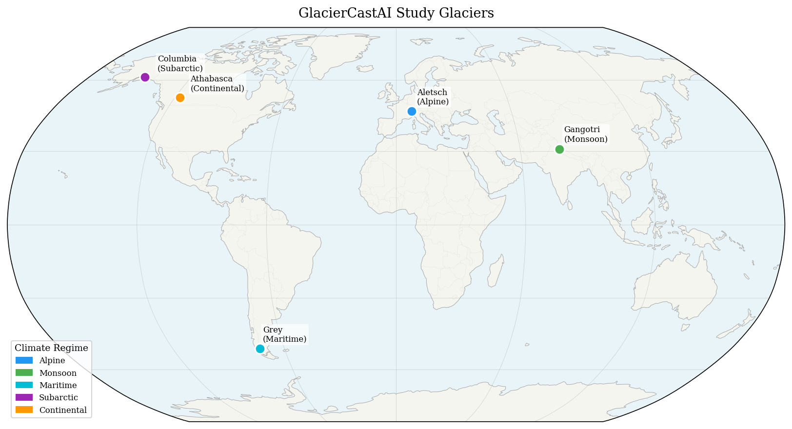
Five glaciers were intentionally selected to span diverse climate regimes rather than maximize dataset size, enabling evaluation of model generalization across Alpine, monsoon-driven, maritime, subarctic, and continental settings (Table 1, Fig. 1).
| Glacier | Region | Climate Regime | Period |
|---|---|---|---|
| Aletsch | Swiss Alps | Alpine | 2002–2023 |
| Gangotri | Himalayas | Monsoon | 2004–2023 |
| Grey | Patagonia | Maritime | 2004–2023 |
| Columbia | Alaska | Maritime/Subarctic | 2001–2023 |
| Athabasca | Canadian Rockies | Continental | 2001–2023 |
3.2 Data Sources↩︎
3.2.1 Satellite Imagery↩︎
Landsat Collection 2 Level-2 surface reflectance products (Landsat 5, 7, 8, and 9) are used, accessed via the USGS Earth Explorer and Microsoft Planetary Computer STAC API. Summer acquisitions (June–September for Northern Hemisphere glaciers; December–March for Grey Glacier, Patagonia) with cloud cover below 20% are selected. Band combinations include Green (Band 3), NIR (Band 5), and SWIR1 (Band 6), from which NDSI is derived as an auxiliary channel (\(\text{NDSI} = (\text{Green} - \text{SWIR1}) / (\text{Green} + \text{SWIR1})\)). The dataset spans 64 scenes across all five glaciers covering 2000–2023.
3.2.2 Climate Data↩︎
ERA5 monthly mean reanalysis data from the Copernicus Climate Data Store [6] provides four variables aggregated to seasonal means: 2m air temperature (t2m), total precipitation (tp), snowfall (sf), and surface net solar radiation (ssr). Four seasons (DJF, MAM, JJA, SON) yield a 16-dimensional climate feature vector per timestep, embedded as a time-varying auxiliary input to the temporal model. Solar radiation values reaching approximately \(18 \times 10^6\) J m\(^{-2}\) are normalized using physical-range standardization to prevent FP16 overflow during mixed-precision training.
3.2.3 Terrain Data↩︎
The Copernicus DEM GLO-30 (30m resolution) provides elevation data from which slope and aspect (decomposed into sine and cosine components to avoid circular discontinuity) are derived. DEM tiles are downloaded via AWS open data, reprojected to UTM, and merged per glacier region.
3.3 Preprocessing Pipeline↩︎
All raster inputs are co-registered to a common UTM grid at 30m resolution. Landsat digital numbers are converted to surface reflectance using Collection 2 scale factors (\(\rho = \text{DN} \times 0.0000275 - 0.2\)). Glacier masks are derived by thresholding NDSI \(> 0.4\).
Patches of \(256 \times 256\) pixels are extracted using a sliding window with 64-pixel overlap, retaining only patches with at least 3% glacier coverage and 70% valid (non-cloud) pixels. This yields 29,810 patches across 64 scenes. Temporal sequences of \(T=4\) consecutive timesteps are constructed per spatial location, paired with target masks at the subsequent timestep. The dataset comprises 40,476 sequences, split temporally to prevent data leakage: test covers 2022–2023, validation covers 2016–2017, and training uses all prior years (train: 27,725; val: 5,861; test: 6,890 sequences).
3.4 Model Architecture↩︎
3.4.1 Spatial Encoder↩︎
A ResNet50 backbone [12] pre-trained on ImageNet encodes each of the \(T=4\) timesteps independently, producing spatial feature maps. The backbone is frozen during the first five epochs (warmup) to prevent randomly-initialized decoder weights from corrupting pretrained representations, then fine-tuned end-to-end.
3.4.2 Temporal Model and Climate Fusion↩︎
Encoded spatial features from all timesteps are passed to a ConvLSTM [10] with three layers (hidden dimension 256, kernel size \(3 \times 3\)). Climate features are provided as a 16-dimensional time-varying input injected at each ConvLSTM step via cross-attention, allowing the model to condition spatial predictions on atmospheric state. The fused spatiotemporal representation is passed to all output heads.
3.4.3 Output Heads↩︎
Three output heads operate on the fused representation: (i) a UNet-style [7] decoder producing per-pixel glacier probability maps (boundary mask head); (ii) an MLP regression head predicting annual area loss at 1, 2, and 3-year horizons (retreat rate head); and (iii) a 3-class MLP classifier for accelerated retreat risk (low/medium/high). In the ablation experiments, the terrain branch (DEM projection layer) is activated or deactivated to isolate its contribution.
3.4.4 Climate-Only MLP Baseline↩︎
To directly test whether climate signals alone carry predictive information, a lightweight climate-only MLP baseline is implemented. This model flattens the \(T \times F = 4 \times 16 = 64\)-dimensional climate sequence and passes it through a three-layer MLP (hidden dimension 256), producing the same three outputs as the full model. The boundary mask is generated at \(64 \times 64\) resolution and bilinearly upsampled to \(256 \times 256\). This model has 661K parameters—approximately 85\(\times\) fewer than the 56.1M-parameter full model—providing a parameter-efficient lower bound for climate-driven forecasting.
3.5 Loss Function↩︎
The combined training objective is: \[\mathcal{L} = \mathcal{L}_{\text{seg}} + \lambda_1 \mathcal{L}_{\text{retreat}} + \lambda_2 \mathcal{L}_{\text{risk}} \label{eq:loss}\tag{1}\] where the segmentation loss combines Dice, binary cross-entropy, and boundary-aware components: \[\mathcal{L}_{\text{seg}} = 0.5\,\mathcal{L}_{\text{Dice}} + 0.3\,\mathcal{L}_{\text{BCE}} + 0.2\,\mathcal{L}_{\text{boundary}}\] The boundary loss upweights pixels within three pixels of the glacier edge by a factor of \(\theta = 19\), penalizing coarse edge predictions. The retreat and risk loss weights are \(\lambda_1 = 0.5\) and \(\lambda_2 = 0.3\).
3.6 Training Details↩︎
All models are trained with AdamW (\(lr = 10^{-4}\), weight decay \(= 10^{-4}\), \(\beta = (0.9, 0.999)\)) with cosine annealing and 5-epoch linear warmup. Mixed-precision training (FP16) is used throughout. Early stopping monitors validation IoU with patience of 15 epochs. Training is performed on an NVIDIA RTX 2060 GPU (6GB VRAM) with batch size 4. All experiments use identical hyperparameters to ensure fair modality comparison. Seeds are fixed at 42 for reproducibility. Results reflect single runs per experimental condition; multi-seed evaluation is an acknowledged limitation and is left for future work.
3.7 SHAP Attribution↩︎
To identify which ERA5 climate variables drive predicted glacier retreat, SHAP KernelExplainer [11] is applied to the exp002 model. Imagery and terrain inputs are held fixed at a reference sample while only the 16-dimensional climate feature vector is perturbed across 50 test patches, using 50 background samples for the explainer and 100 perturbation samples per prediction. SHAP values are averaged over the \(T=4\) timesteps to obtain a single attribution score per climate feature.
4 Experiments↩︎
4.1 Evaluation Metrics↩︎
Two primary metrics are reported:
IoU: Intersection-over-Union of predicted versus ground-truth glacier mask, evaluated at a threshold of 0.5. Measures overall segmentation accuracy.
BF1: Boundary F1, computed as the harmonic mean of precision and recall evaluated exclusively on glacier edge pixels (dilation width of 3 pixels). Captures boundary delineation quality independent of interior accuracy.
4.2 Baselines↩︎
The proposed method is compared against two traditional forecasting baselines computed on the same test set:
B1 — Persistence: predicts the next glacier boundary as identical to the current observed boundary (NDSI threshold \(> 0.4\) on the last input timestep). Represents the null hypothesis that glaciers do not change.
B2 — Linear trend: fits a pixel-wise linear regression over the \(T=4\) input NDSI values and extrapolates one step forward. Represents the assumption of steady linear retreat.
4.3 Ablation Design↩︎
Following the pre-registered protocol, four conditions are compared, varying only the input modalities while holding all other hyperparameters fixed:
exp001 — Image only: imagery branch active; climate and DEM branches disabled.
exp002 — Image + Climate: imagery and ERA5 climate active; DEM disabled.
exp003 — Image + Climate + DEM: all three modalities active.
exp005 — Climate only (MLP): lightweight MLP on ERA5 features only; no imagery or DEM.
Each experiment uses an isolated checkpoint directory to prevent result contamination, verified before training via directory inspection. Climate features are confirmed non-zero via batch-level diagnostic prior to each run.
5 Results↩︎
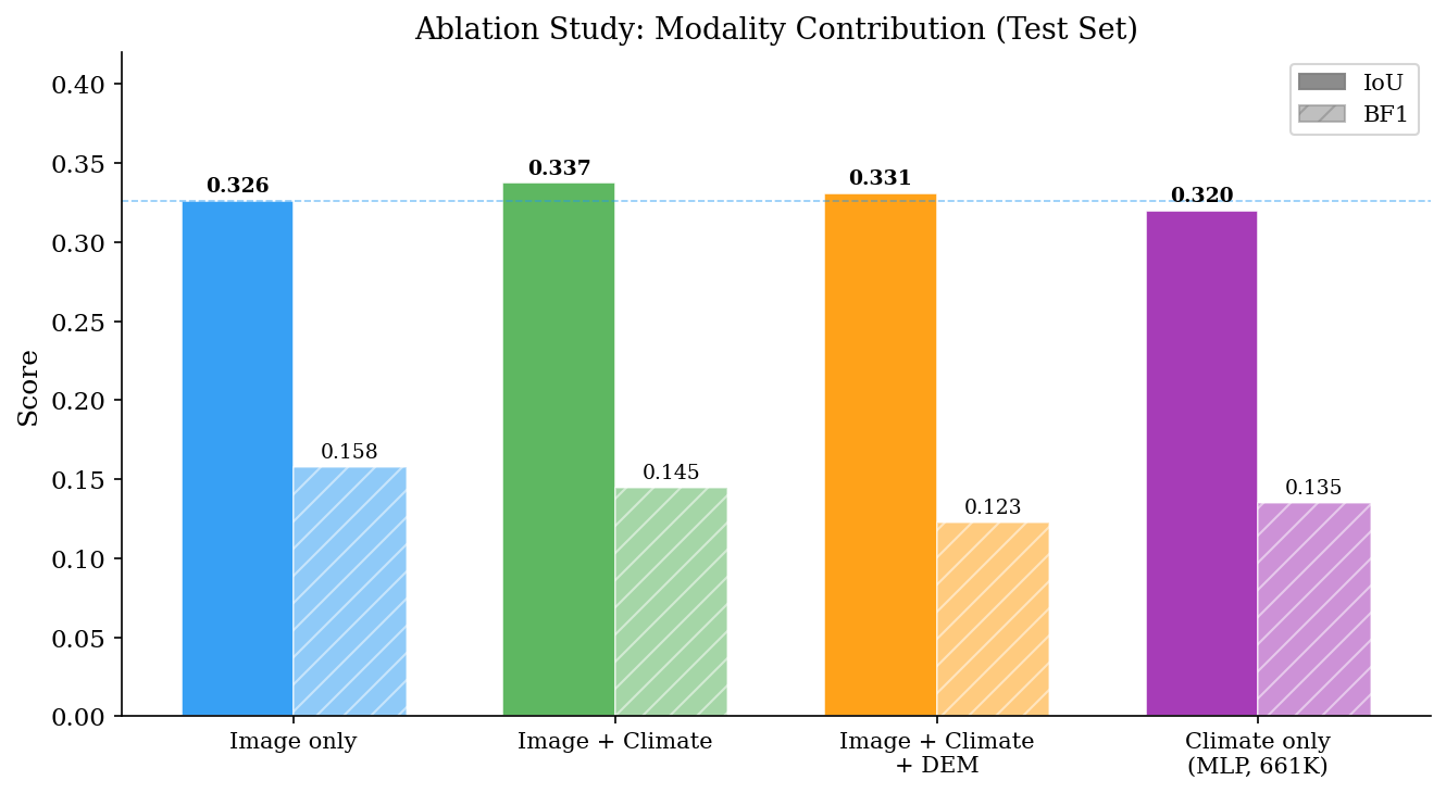
Table 2 presents results on the held-out test set (2022–2023), including traditional baselines. Fig. 2 visualizes the IoU and BF1 comparison across all conditions.
| Model | Params | IoU \(\uparrow\) | BF1 \(\uparrow\) |
|---|---|---|---|
| B1: Persistence | N/A | 0.160 | 0.128 |
| B2: Linear trend | N/A | 0.169 | 0.147 |
| exp001: Image only | 56.1M | 0.326 | 0.158 |
| exp002: + Climate | 56.1M | 0.337 | 0.145 |
| exp003: + Climate + DEM | 56.1M | 0.331 | 0.123 |
| exp005: Climate only | 0.66M | 0.320 | 0.135 |
5.1 Comparison Against Traditional Baselines↩︎
All deep learning models substantially outperform both traditional baselines. The persistence baseline achieves an IoU of 0.160, and the linear trend baseline achieves 0.169. The weakest deep learning model (exp005 climate-only MLP, IoU 0.320) improves over linear trend by 89% relative, and the best model (exp002, IoU 0.337) improves by 99% relative. This is consistent with the models learning meaningful temporal dynamics rather than simply extrapolating static patterns.
5.2 Effect of Climate Signals↩︎
Adding ERA5 climate features (exp002) improves IoU from 0.326 to 0.337 (+3.4% relative) over the image-only baseline, suggesting that atmospheric forcing variables carry predictive information beyond what Landsat imagery alone provides. This improvement is consistent with the hypothesis that climate signals precede visible glacier boundary change.
5.3 Effect of Terrain Features↩︎
Adding DEM features to the climate-augmented model (exp003, IoU 0.331) yields a slight regression compared to exp002. One possible explanation is that static terrain features (slope, aspect) are already implicitly encoded in the spatial patterns of the Landsat imagery, making their explicit inclusion redundant at the patch level. This finding suggests that terrain features may require more careful integration—for example, as conditioning variables for the climate encoder rather than additive spatial features.
5.4 Climate-Only Baseline↩︎
The climate-only MLP (exp005) achieves an IoU of 0.320—98% of the image-only baseline (0.326) while using 85\(\times\) fewer parameters (661K vs.56.1M). ERA5 seasonal climate variables alone, with no access to Landsat imagery, are nearly sufficient to predict glacier boundary positions at the patch level. This result is consistent with the hypothesis that climate signals encode substantial predictive information about glacier retreat that precedes visible imagery change.
5.5 Per-Glacier Analysis↩︎
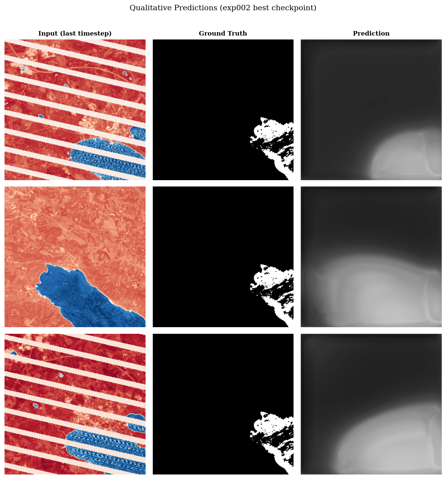
Table 3 reports per-glacier IoU for exp002 on the test set. Fig. 3 shows qualitative predictions for representative test patches. Columbia Glacier (Alaska) achieves the highest IoU (0.500), likely reflecting its large area and strong, consistent retreat signal. Athabasca Glacier (IoU 0.045) performs poorly, consistent with its small area (17.8 km\(^2\)) and the challenge of predicting fine-scale boundaries from coarse ERA5 climate signals ( 31km resolution). Gangotri Glacier has no test sequences due to its scenes falling entirely within the training years under the temporal split.
| Glacier | IoU | Std | \(n\) patches |
|---|---|---|---|
| Columbia | 0.500 | 0.372 | 200 |
| Grey | 0.250 | 0.201 | 200 |
| Aletsch | 0.122 | 0.187 | 200 |
| Athabasca | 0.045 | 0.110 | 200 |
| Gangotri | — | — | 0 (training split) |
5.6 SHAP Climate Attribution↩︎
Table 4 reports mean absolute SHAP values for the 16 ERA5 climate features, computed on 50 test patches using the exp002 model. Figs. 4 and 5 visualize the attribution by feature and by variable group and season.
Spring solar radiation (SolarRad_MAM) is the highest-ranked driver, followed by spring snowfall (Snowfall_MAM) and summer solar radiation (SolarRad_JJA). Aggregated by variable group, solar radiation accounts for the largest share of attribution, followed by snowfall and precipitation. Temperature (T2m) contributes the least, which may reflect its correlation with solar radiation variables from which the model captures a similar signal.
| Feature | Mean \(|\)SHAP\(|\) | Rank |
|---|---|---|
| SolarRad_MAM | 0.0012 | 1 |
| Snowfall_MAM | 0.0004 | 2 |
| SolarRad_JJA | 0.0003 | 3 |
| Snowfall_DJF | 0.0001 | 4 |
| Precip_MAM | 0.0001 | 5 |
| Attribution by variable group (aggregated) | ||
| Solar Radiation | 0.0004 | — |
| Snowfall | 0.0002 | — |
| Precipitation | 0.0001 | — |
| Temperature | 0.0000 | — |
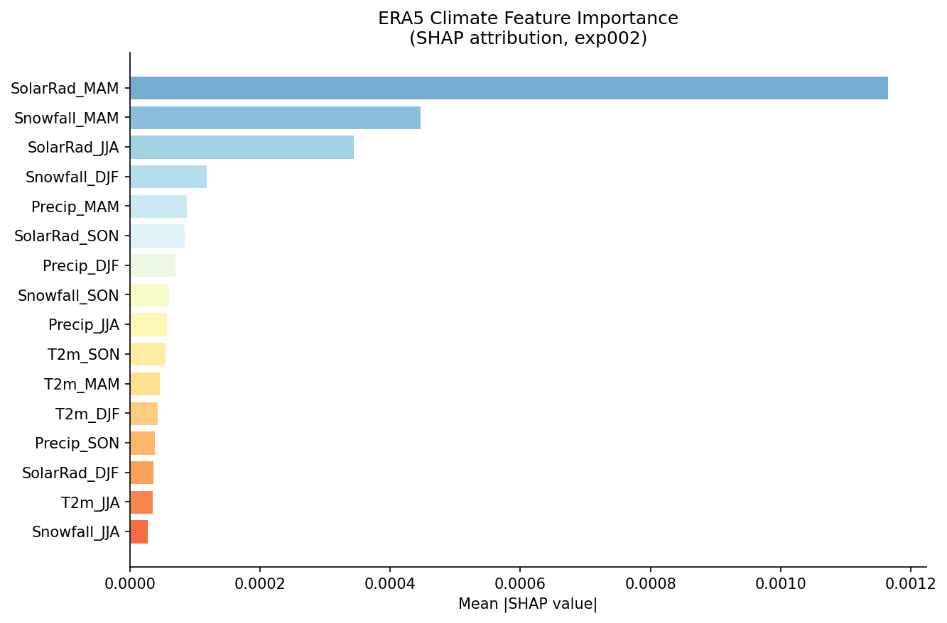

The prominence of spring solar radiation is physically interpretable: the onset and intensity of the melt season is primarily driven by incoming shortwave radiation in spring (MAM), which influences how early and how extensively the seasonal snowpack begins to melt. This signal precedes the visible retreat of the glacier terminus by weeks to months, consistent with the temporal lag hypothesis motivating this work. The secondary importance of spring snowfall reflects its role in replenishing the snowpack and modulating the effective melt season length.
5.7 Discussion↩︎
The absolute IoU values (0.320–0.337) are not directly comparable to state-of-the-art glacier mapping models such as GlaViTU (IoU \(> 0.85\)) [4], because forecasting future boundaries from historical sequences is inherently more uncertain than delineating current boundaries from high-quality imagery. The relevant comparisons are between experimental conditions and traditional baselines, both of which GlacierCastAI substantially exceeds.
The high variance in per-glacier performance (Columbia 0.500 vs.Athabasca 0.045) reveals a likely size dependence: larger glaciers with stronger retreat signals appear better predicted. This is consistent with the spatial resolution mismatch between ERA5 climate data ( 31km) and the 30m Landsat patches — fine-scale climate variability relevant to small glaciers may be smoothed out at ERA5 resolution. Future work should investigate glacier-specific fine-tuning or area-weighted loss functions to address this disparity.
A further limitation is that results reflect single training runs per experimental condition, and multi-seed evaluation has not been performed due to computational constraints. Variance across seeds and bootstrap confidence intervals represent important directions for strengthening the statistical claims of this work.
6 Conclusion↩︎
This paper presented GlacierCastAI, which reframes glacier boundary prediction as a multi-modal spatiotemporal forecasting problem rather than a mapping problem. Through a pre-registered ablation across four experimental conditions, compared against traditional baselines and interpreted via SHAP attribution, the results suggest that:
All deep learning models substantially outperform persistence and linear trend baselines, improving IoU by 89–99% relative, consistent with the models learning meaningful temporal dynamics.
ERA5 climate signals improve glacier retreat forecasting IoU by 3.4% over imagery alone, suggesting that atmospheric forcing provides predictive information not captured by Landsat sequences.
A climate-only MLP with 661K parameters achieves 98% of image-only performance, suggesting that ERA5 seasonal variables are nearly sufficient for patch-level glacier boundary forecasting.
DEM terrain features slightly reduce performance when added to imagery and climate inputs, suggesting redundancy with spatially encoded imagery features at the current patch scale.
SHAP attribution identifies spring solar radiation (MAM) as the highest-ranked climate driver, followed by spring snowfall and summer solar radiation, consistent with the role of spring insolation in setting melt season trajectories.
These results are consistent with the hypothesis that climate signals precede visually detectable glacier boundary change, supporting the feasibility of climate-driven early warning systems for glacier retreat. Future work will address multi-seed evaluation to quantify result variance, per-glacier fine-tuning to reduce the size-dependence of forecast accuracy, integration of higher-resolution regional climate data to improve small-glacier performance, and extension to longer forecast horizons.