Introduction

— Quantum advantage, the outperformance of quantum computers over classical digital computers on certain tasks, is considered one of the most important milestones in quantum computation. Random circuit sampling (RCS) is regarded as a primary benchmark for demonstrating quantum advantage on current noisy intermediate-scale quantum computers. Claims of quantum advantage in RCS have recently been reported using superconducting qubits [1]–[5] and ion-trap qubits [6]–[8]. Operationally, RCS is the task of sampling bitstrings from a Haar-random quantum state, hereafter referred to as a random quantum state, generated by a random quantum circuit [9]. RCS is believed to be classically intractable because a random quantum state is highly entangled [10] and appears too chaotic for a classical algorithm to exploit any pattern or structure [11]–[14]. Statistical properties of output bitstrings such as the exponential distribution, the linear cross-entropy benchmark [1], [9], [15], [16], heavy output generation [17] and anti-concentration [18]–[20] have been proposed as evidence for the quantum advantage of RCS.

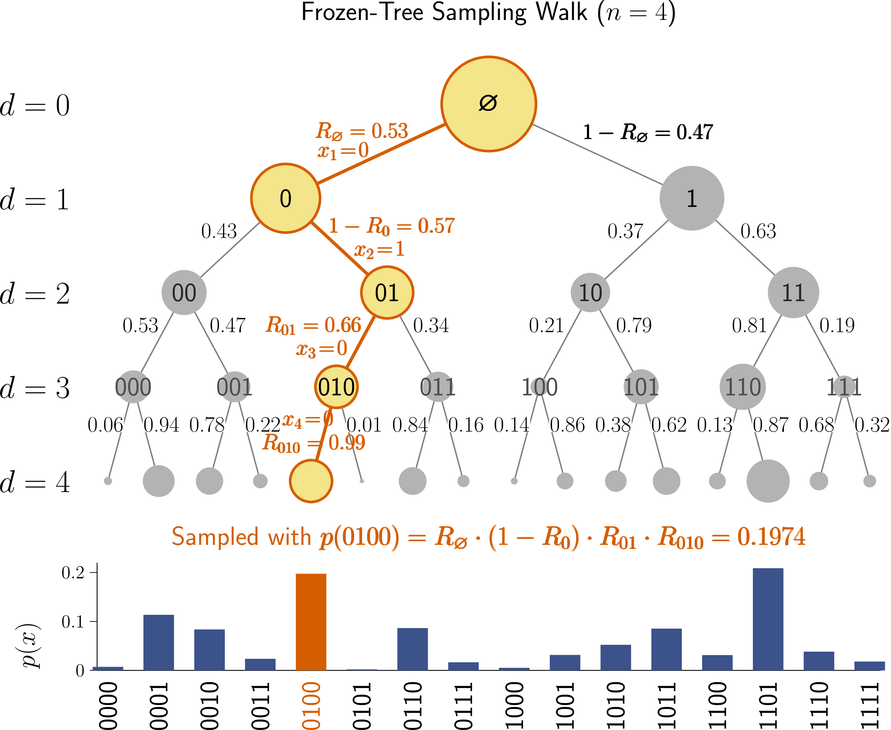
In this paper, we challenge the premise of quantum advantage in RCS by introducing frozen-tree sampling, which exploits the exact conditional scale invariance of a random quantum state [21], [22], as shown in Fig. 1. We prove that the probability of finding bitstrings of a random quantum state can be represented by a binary tree with a precise recursive structure: each bit is drawn from a Beta-distributed conditional probability determined by the preceding bits. We present a frozen-tree sampler that classically samples bitstrings from an \(n\)-qubit random quantum state in \(O(n)\) time per sample. Both the probability \(p_C(x)\) of a random quantum circuit and the probability \(p_F(x)\) of the frozen-tree sampler are independent realizations of the Dirichlet vector characterizing a random quantum state, and are therefore statistically identical. It follows that no statistical verification method can serve as evidence of quantum advantage in RCS.

Dirichlet distribution of a Haar-random quantum state

— A random pure quantum state of \(n\) qubits in an \(N=2^n\) dimensional Hilbert space [23] is written as \[\begin{align} \ket{\psi} = \sum_{x=0}^{N-1} c_x \ket{x}\,, \end{align}\] where the bitstring \(x=x_1\cdots x_n\) with \(x_i\in \{0,1\}\) runs from \(0\) to \(N-1\) and each amplitude \(c_x\) is sampled from the complex normal distribution, \(c_x \sim {\cal CN}(0,1)\). The probability of finding bitstring \(x\) is given by \(p(x) = \abs{c_x}^2/\sum_y \abs{c_y}^2\). The probability vector \(\boldsymbol{p}= (p(x))_{x=0,\dots N-1}\) follows a flat Dirichlet distribution on the \(N-1\) simplex [24] \[\begin{align} \left(p(x)\right) \sim \text{Dir}(1,\dots,1)_{2^n}\,. \end{align}\] The marginal distribution \(p(x)\) follows a Beta distribution, \(p\sim \text{Beta}(1,N-1)\), which becomes an exponential distribution in the rescaled random variable \(Np\) in the limit of large \(N\) [25], [26]. A quantum computer realizes a random quantum state by applying a circuit \(C\), chosen randomly according to the Haar measure, to an input state, \(\ket{\psi} = C\ket{0^{n}}\), and performs a measurement in the computational basis to sample a bitstring \(x\) from the probability distribution \(p_C(x) = \abs{\bra{x}C\ket{0^n}}^2=\abs{c_x}^2/\sum_y|c_y|^2\). Note that a random circuit \(C\) yields a single realization of the Dirichlet distribution, \(\boldsymbol{p}_C = (p_C(x)) \sim \text{Dir}(1,\dots,1)\).

Binary-tree representation of \(p(x)\)

— The output bitstrings of RCS appear so random that no pattern or correlation is readily discernible. Indeed, they pass the NIST statistical test for randomness [27]–[30]. Consider, for example, two \(n=5\) bitstrings, \(01101\) and \(01100\), obtained from RCS. Both share the same four-bit prefix \(u=x_1x_2x_3x_4 = 0110\), but differ in the final bit, \(x_5 \in \{0,1\}\). The central question of this paper is: given the prefix \(u=x_1x_2x_3x_4=0110\), what is the probability of obtaining \(x_5 =0\) or \(x_5=1\)? To answer it, we exploit the conditional scale invariance of a random quantum state established in Refs. [21], [22]. A random quantum state is not disordered but conceals an exact self-similar symmetry, as shown in Fig. 1. This makes it possible to express \(p(x)\) as a binary tree with an analytic split probability at each depth and to sample bitstrings classically in \(O(n)\) per sample.

As shown in Figs. 1 and  2, Theorem 1 represents the probability \(p(x)\) of finding bitstring \(x\) for a random state as a binary tree walk from the root to leaves. The universal statistics of RCS is the Beta distribution. The full leaf probability \(p(x)\) follows \(\text{Beta}(1,N-1)\), which becomes exponential in the limit of large \(N\). More generally, for any prefix \(u\) (with \(x=uw\)), the subtree mass \(P_u\equiv\sum_w p(uw)\), the weight of one subtree relative to the whole tree, follows \(P_u\sim\mathrm{Beta}(S_d,N-S_d)\), where \(S_d=2^{n-d}\) is the number of leaves in the subtree at depth \(d\) [21]. For an internal node \(u\) with children \(u0\) and \(u1\), the mass splits as \(P_u=P_{u0}+P_{u1}\), and the pair satisfies \((P_{u0},P_{u1})\sim\mathrm{Dir}(K,K)\) with \(K=S_2/2 = 2^{n-d-1}\). The split ratio in Eq. (1 ) can then be written as \(R_u \equiv {P_{u0}}/{P_u} \sim \text{Beta}(K,K)\), so that \(P_{u0} = R_uP_u\) and \(P_{u1} = (1-R_u)P_u\). For \(R_u\sim \mathrm{Beta}(K,K)\), the mean and standard deviation are \[\begin{align} \mathbb{E}[R_u] =\frac{1}{2} \,,\quad \sigma_d =\frac{1}{2\sqrt{2K+1}} \,, \label{Variance} \end{align}\tag{2}\] Eq. (2 ) shows that the fluctuation of the split ratio depends only on the depth \(d\) through \(K=2^{n-d-1}\). Near the root \((K\gg 1)\) the branching ratio concentrates at \(1/2\) with vanishing spread, \(\sigma_d\to 0\), whereas near leaves \((K\approx 1)\) it is nearly uniform on \([0,1]\). Because \(\sigma_d\) is a universal, depth-dependent quantity, it distinguishes ideal RCS from noisy RCS. As discussed below, we define the branch-ratio fidelity \(F_\sigma \equiv \sigma_d^{\rm sample}/\sigma_d^{\rm ideal}\) as the ratio of the empirical branch fluctuation of the samples to its ideal value.

Frozen-Tree Sampling Algorithm

— Once all split ratios \(\{R_u\}\) are fixed, the leaf probability \(p(x)\) is uniquely determined and corresponds to a single realization of a Dirichlet vector, that is, the Born probability of a random quantum state. We therefore propose a frozen-tree sampler that draws each split ratio \(R_u\) once, stores it, and reuses it whenever a later sample revisits the same node. As shown in Fig. 2, the sampler performs a random walk of \(n\) steps from the root to a leaf, making one Bernoulli branch decision with probability \(R_u\) and selecting the bit value \(x_k\) at each node. This requires only \(O(n)\) steps per sample, rather than the exponential resources of storing the full amplitude vector. For \(M\) samples the total runtime is \(O(Mn)\). The sampler produces a genuine Dirichlet realization of a random quantum state because the recursive Beta rule is precisely the recursive representation of a symmetric Dirichlet vector, \(p_F(x)=\abs{\braket{x}{\psi}}^2 = \prod_{k=1}^n R_{x<k}^{1-x_k}(1-R_{x<k})^{x_k}\).

As Fig. 2 depicts a random walk from the root to a leaf, the algorithm draws one bitstring as follows: (1) start at the root \(u=\varnothing\) with depth \(d=0\); (2) look up the branch ratio \(R_u\) if the node has not been visited before, draw \(R_u\sim\mathrm{Beta}(K,K)\) and store it; (3) sample \(x_k=0\) with probability \(R_u\) or \(x_k=1\) with probability \(1-R_u\); (4) move to the child node \(u0\) or \(u1\); (5) repeat until depth \(d=n-1\). This yields one sample from the fixed distribution \(p_F(x)\), where the subscript \(F\) denotes a single frozen tree with all branch ratios \(\{R_u\}\) fixed. The \(2^{n}-1\) branch ratios need not be generated in advance. Instead, we use lazy generation: the first time the sampler visits a node \(u\), it draws \(R_u\) and stores it in a dictionary, reusing it on all subsequent visits, so that only the actually visited nodes are ever instantiated.

The frozen tree needs one frozen split ratio \(R_u\) per node, drawn once and identical every time a sample passes through node \(u\). Storing every visited ratio incurs a memory cost that becomes prohibitive for large \(n\). This is resolved by generating \(R_u\) on demand, deterministically, from the node’s identity (its prefix \(u\)) together with a global seed as \[\begin{align} u \;\xrightarrow{\;\mathrm{PRF(seed},u)\;}\; X_u \sim \mathrm{Unif}[0,1) \;\xrightarrow{\;f_K\;}\; R_u\,, \end{align}\] where the pseudo-random function (PRF) is a keyed, deterministic, stateless map from \((\text{seed},u)\) to a uniform word \(X_u\in[0,1)\), implemented with a hash function such as SHA-256 [33] or a counter-based random number generator (CBRNG) [34]. The map \(f_K\) transforms \(X_u\) into a Beta variate \(R_u\sim\mathrm{Beta}(K,K)\), \[\begin{align} f_K(X_u)=\begin{cases} \dfrac{1}{2}, & K>2^{102}\\[6pt] \dfrac{1}{2}+\sigma_K\,\Phi^{-1}(X_u), & 2^{9}\le K\le 2^{102}\\[6pt] \dfrac{\Gamma_K}{\Gamma_K+\Gamma_K'}, & K<2^{9} \end{cases}\,, \end{align}\] where \(\Phi^{-1}\) is the inverse standard-normal CDF, mapping a uniform variate to a Gaussian one. Here \(\Gamma_K,\Gamma_K'\) are independent \(\mathrm{Gamma}(K,1)\) variates. The three regimes exploit the depth dependence of the branch-ratio spread \(\sigma_K=1/\sqrt{4(2K+1)}\). Near the root \((K>2^{102}\), i.e., \(n-d>103\)), \(\sigma_K\) falls below the FP64 machine epsilon, \(\sigma_K<2^{-52}\), so \(R_u=1/2\) to machine precision. No PRF call is needed and the cost is \(O(1)\). In the intermediate regime \((2^{9}\le K\le 2^{102}\), i.e., \(10< n-d\le 103\)), the Beta distribution is Gaussian to high accuracy, and a single inverse-CDF evaluation yields \(R_u\) at \(O(1)\) cost. Near the leaves (\(K<2^{9}\), i.e., \(n-d\le 10\)), \(R_u\) is drawn from the exact Gamma ratio at \(O(K)\) cost, or via Cheng’s acceptance-rejection algorithm [35] at \(O(1)\) cost.

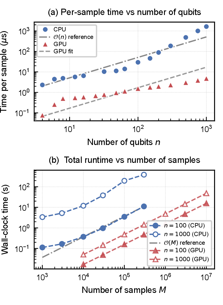
Fig. 3 shows the \(O(n)\) scaling per sample of the frozen-tree sample code [36]. It samples \(M=10^7\) bitstrings of an \(n=1000\)-qubit random state on the GPU in a few seconds. For comparison, the Google Sycamore processor required about 200 seconds to collect \(\sim\!10^6\) samples at \(n=53\) [1], [37]. The frozen-tree sampler is fast, exact, and noiseless. Fig. 3 (a) confirms the predicted \(O(n)\) per-sample time on CPU and GPU. Fig. 3 (b) shows the total runtime scaling as \(O(Mn)\).

The frozen tree samples bitstrings from the probability \(p_F(x)\) of a random state \(\ket{\psi}\) characterized by its branching ratios \(\{R_u\}\), \[\begin{align} p_F(x)=\abs{\braket{x}{\psi}}^2=\prod_{k=1}^n R_{x_{<k}}^{1-x_k}\bigl(1-R_{x_{<k}}\bigr)^{x_k}\,, \end{align}\] while a random circuit \(C\) samples from the probability \(p_C(x)\) of another random state \(\ket{\varphi}=C\ket{0^n}\), \[\begin{align} p_C(x)=\abs{\bra{x}C\ket{0^n}}^2\,. \end{align}\] Both \(p_F(x)\) and \(p_C(x)\) are independent instances of the flat Dirichlet distribution on the \((N-1)\)-simplex that any random state must obey. They are therefore statistically identical, \(p_F(x)\stackrel{d}{=}p_C(x)\), even though \(p_F(x)\ne p_C(x)\) in general. The only remaining unknown is the map between a circuit \(C\) and the branching ratios \(\{R_u\}\). Consequently, insofar as RCS is regarded as the task of drawing bitstrings from the Dirichlet distribution of a random state, the classical frozen-tree sampler, at \(O(n)\) cost per sample, reproduces all statistical properties used to certify RCS. Thus no such statistic can serve as evidence of quantum advantage in RCS.

Noisy Frozen-Tree Sampler

— The frozen-tree sampler readily accommodates various noise channels: global depolarizing noise, local depolarizing noise, amplitude damping, and readout error, at the same \(O(n)\) cost, with each channel modeled at a distinct stage of the tree. Global depolarizing noise is an affine transformation of the Dirichlet vector [21]: the noisy leaf probability is a mixture of the ideal probability and the uniform distribution, \[\begin{align} \widehat{p}(x) = F\,p_{\text{ideal}}(x) + \frac{1-F}{2^n}\,, \end{align}\] where \(F\) is the circuit fidelity. This is exact at any \(n\) and requires no noise-trajectory sampling.

Readout error and amplitude damping act qubit-by-qubit on the completed bitstring, after the tree path is fixed. A true string \(x_k\) is corrupted into an observed string \(y_k\) through per-qubit confusion matrices \({C_k(y_k \mid x_k)}\), so the observed-string probability is \[\begin{align} \widehat{p}(y) = \sum_{x} p_{\text{ideal}}(x)\prod_{k=1}^n C_k(y_k\mid x_k)\,. \label{Eq:noisy95tree} \end{align}\tag{3}\] For readout error, the confusion matrix is \[\begin{align} C_k = \begin{pmatrix} P(0\mid 0) & P(0\mid 1)\\[4pt] P(1\mid 0) & P(1\mid 1) \end{pmatrix} = \begin{pmatrix} 1-\epsilon^{01}_k & \epsilon^{10}_k\\[4pt] \epsilon^{01}_k & 1-\epsilon^{10}_k \end{pmatrix}\,, \end{align}\] where \(P(0\mid 1) =\epsilon^{10}_k\) (\(P(1\mid 0) =\epsilon^{01}_k\)) is the probability that 1 (0) of the \(k\)-th qubit is incorrectly measured as 0 (1). Amplitude damping is a one-sided decay from \(\ket{1}\) to \(\ket{0}\) at rate \(\gamma_k = 1-\exp(-t_{\text{meas}}/T_{1,k})\), where \(T_{1,k}\) is the relaxation time of qubit \(k\) and \(t_\text{meas}\) is the measurement window. Its confusion matrix is \[\begin{align} C_k =\begin{pmatrix} 1 & \gamma_k \\ 0 & 1-\gamma_k \end{pmatrix}\,. \end{align}\] The exact evaluation of Eq. (3 ) is feasible only at enumerable sizes \((n\lesssim 25)\). For larger \(n\), the confusion matrices are instead folded into each conditional branch probability, preserving the \(O(n)\) cost.

Fig. 4 shows how the branch ratio \(R_u\) fluctuates with node depth \(d\) for the frozen tree, the Google Sycamore data [37], and a classical uniform-random-bit sample. Fig. 4 (b) confirms that the frozen-tree spread follows \(\sigma_d=1/(2\sqrt{2K+1})\) exactly, whereas Sycamore lies between ideal RCS and classical random bits, with \(R_u\) fluctuating more strongly toward the leaves. Fig. 4 (c) shows the frozen tree gives \(\hat{F}=1\) across all depths, while Sycamore saturates at \(\hat{F}=0.418\).

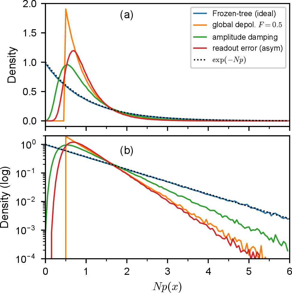
Figure 5 plots the distributions \(\mathrm{Pr}(p)\) of bitstring probabilities, scaled as \(Np\), for \(n=20\) under global depolarizing noise \((F=0.5)\), amplitude damping \((\gamma_k=0.05)\), and readout error (\(\epsilon^{01}=0.02, \epsilon^{10}=0.06)\). A notable feature of the frozen-tree is that these noisy distributions are obtained by enumerating all \(2^n\) leaves and applying each channel operator, without sampling bitstrings. Because \(p(x)\) is given in closed form as a product of branch ratios, the full leaf-probability vector \(\pmb{p}=(p(x))\) is computed exactly, and each physical noise channel acts as a linear map on it. This contrasts with the conventional analysis of RCS, in which the noisy output distribution can only be estimated by drawing many bitstrings and histogramming them with estimation error. Like \(\mathrm{Pr}(p)\), every sample-based verification tool, such as cross-entropy, heavy-output generation, and anticoncentration, is a functional of \(p\) and is therefore exactly determined rather than empirically estimated. As shown in Fig. 5, amplitude damping and readout error suppress the exponential peak and deplete the small \(Np\) region relative to the ideal law \(\exp(-Np)\), whereas global depolarizing noise leaves the exponential shape intact but rescaled and shifted to the right by the fidelity \(F\) [21]. Amplitude damping (green) retains a heavier tail than either depolarizing noise or readout error, remaining well above them and falling off only near \(Np\approx6-7\); this is the signature of a one-sided channel, which concentrates probability and preserves more of the exponential tail. Depolarizing noise (orange) and readout error (red) decay faster, essentially vanishing by \(Np\approx 4-5\), since they move probability mass away from the high \(Np\) leaves. These are the same statistical distortions seen in the Google Sycamore data [21]. The frozen-tree sampler thus reproduces not only the ideal exponential distribution but also its realistic noisy statistics exactly. This implies that no test acting on samples alone can distinguish the frozen-tree sampler from a quantum random circuit.

Summary and Discussion

— We have shown that the probability \(p(x)=\abs{\braket{x}{\psi}}^2\) of finding bitstring \(x\) in a random state \(\ket{\psi}\) is represented by a binary tree whose branching ratios \(R_u\) follow the Beta distribution \(\mathrm{Beta}(K,K)\), a direct consequence of the exact conditional scale invariance of random states [21], [22]. Through random walks from the root to leaves, the frozen-tree sampler draws bitstrings from the Born distribution of an \(n\)-qubit random state in \(O(n)\) time per sample. It generates \(10^7\) samples at \(n=1000\) within seconds on a personal computer. It accommodates depolarizing noise, amplitude damping, and readout error at the same cost.

The probability vector \(\boldsymbol{p}=(p(x))\) of any random state is a flat Dirichlet vector on the simplex. A random circuit produces one such vector and the frozen-tree sampler produces another; the two are independent realizations of the same distribution, and statistically identical \(p_F(x)\stackrel{d}{=}p_C(x)\) while \(p_F(x)\ne p_C(x)\). It follows that any verification method built from the leaf-probability \(p\) such as the exponential distribution, anticoncentration, linear XEB, and heavy-output generation, takes the same value for the frozen-tree sampler as for a random quantum circuit. Since the frozen tree reproduces all of these classically in \(O(n)\) time, none of them can by itself certify quantum advantage. They are necessary features of the Dirichlet ensemble that a classical sampler shares, not sufficient evidence of hardness.

Any surviving quantum advantage of RCS must therefore reside in the circuit-specific realization \(p_C(x)\), the map from a given circuit to its amplitudes, rather than in the sampled statistics. Whether even this residual survives is the subject of our companion work [38], which constructs a Hurwitz–frozen-tree circuit \(C_F\) implementing \(p_{C_F}(x)=\abs{\bra{x}C_F\ket{0^n}}^2=p_F(x)\): a quantum circuit whose output is, by construction, classically sampled in \(O(n)\) time. Such a family shows that a circuit can pass the RCS benchmark while admitting an efficient classical sampler, underscoring that the benchmark’s statistics do not witness advantage. Taken together, these results argue that random circuit sampling, as currently verified, is not a sound stand-alone benchmark for quantum advantage.

1 Appendix: Verification statistics as functionals of the leaf law↩︎

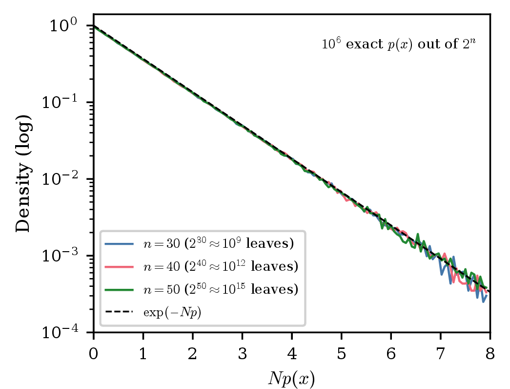
The exact-enumeration results of the main text are limited to \(n\lesssim 25\), where the full \(2^n\) probability vector can be constructed. To confirm that the frozen-tree sampler reproduces the exponential leaf statistics in the regime relevant to hardware experiments, we draw \(10^{6}\) leaves uniformly from the \(2^{n}\) possible bitstrings at \(n=30\), \(40\), and \(50\), and evaluate each leaf probability \(p(x)\) in closed form from its branch ratios. Because \(p(x)\) is computed directly rather than estimated from finite-frequency counts, no sampling error enters the individual probabilities; the only randomness is in which leaves are drawn. As shown in Fig. 6, the histograms of the rescaled variable \(Np(x)\) coincide with the ideal law \(\exp(-Np)\) at every size, even though \(10^{6}\) leaves represent a vanishing fraction—from \(10^{-3}\) at \(n=30\) down to \(10^{-9}\) at \(n=50\)—of the full distribution. The distribution \(\Pr(Np)\) shown here is built from this finite set of \(10^{6}\) computed values of \(p(x)\), far smaller than the total number of leaves \(2^{n}\) (\(10^{6}\ll 2^{50}\approx 10^{15}\) at \(n=50\)), yet the exponential law is fully recovered. The leaf law is therefore a property of the flat Dirichlet ensemble, recovered by the \(O(n)\) sampler at scales where direct enumeration is infeasible.

References↩︎