Directional Curvature from Armijo Backtracking:
A Low-Cost Sharpness Probe and a Calibration-Free
Learning-Rate Safeguard for Adam
July 04, 2026
Abstract
The local sharpness of the loss, the top Hessian eigenvalue \(\lambda_1\), determines the largest stable gradient step, but measuring it normally requires Lanczos or Hessian-vector iterations. We observe that a single Armijo backtracking line search already carries this information at the cost of a few forward passes: the accepted step \(\alpha\) brackets the directional curvature \(q = g^\top H g/\|g\|^2\) within the multiplicative band set by the backtracking factor. Across CIFAR-10, Fashion-MNIST and Imagenette, \(\log\alpha\) tracks \(\log\lambda_1\) at Pearson \(-0.91\) to \(-0.95\), giving a low-cost online Edge-of-Stability reading. Used once at initialisation, this measurement yields a learning-rate cap (a safeguard, not a faster optimiser) that makes Adam robust to a too-large initial learning rate across more than three orders of magnitude (\(10^{-3}\) to \(3.0\)), at about one percent overhead, and it is a no-op when the chosen rate is already safe. One probe is enough: periodic in-training probing adds no robust benefit. The raw-gradient probe exposes the mechanism but needs a safety factor calibrated to the architecture by a one-minute divergence sweep. Probing along Adam’s own update direction removes this calibration: a single fixed safety factor \(\kappa = 2\) avoids divergence on all nine architectures we test and across the full learning-rate grids of all four benchmarks, and the recipe transfers to AdamW unchanged.
1 Introduction↩︎
Adam [1] and its variants (AdamW [2], NAdam [3], AMSGrad [4]) are the workhorses of contemporary deep learning. Their per-parameter adaptive scaling absorbs much of the heterogeneity of neural-network gradients and, in practice, decouples optimisation from the worst aspects of architecture-specific gradient geometry. What they do not absorb is the user’s choice of initial learning rate. An \(\eta\) chosen one order of magnitude too large drives the loss to numerical infinity within a handful of steps, well before Adam’s running estimates of the second moment have accumulated enough mass to dampen the update. The result is a single divergent first step, after which the entire training run is wasted.
The community has developed several pragmatic responses to this problem. The most principled is the explicit learning-rate range test [5], [6], which trains a model for one or more epochs while sweeping the learning rate and inspects the loss–learning-rate curve for the largest still-stable value. A second line of work removes the learning rate from the user interface entirely by inferring it from running estimates of online-convex-optimisation quantities; D-Adaptation [7], Prodigy [8], Mechanic [9] and the Schedule-Free family [10] are the most recent and most visible representatives. A third, far less elegant but in practice ubiquitous approach is for users to manually iterate over a few candidate values and to discard whatever diverges. None of the three provides a low-cost, calibrate-once safety check that a particular chosen \(\eta\) is safe.
We propose a fourth route, designed to coexist with rather than replace any of the above. Before the first Adam update, we run a single Armijo backtracking line search [11] at the randomly initialised parameters: starting from \(\alpha = 1\), we backtrack along the negative initial gradient until the standard sufficient-decrease condition is satisfied. The resulting step size \(\bar\alpha_{\text{init}}\) is a one-batch empirical estimate of the largest stable gradient step at initialisation. If the user’s \(\eta_{\text{init}}\) exceeds \(\kappa\cdot \bar\alpha_{\text{init}}\) for a small safety constant \(\kappa\), the optimiser silently lowers \(\eta_{\text{init}}\) to \(\kappa\cdot \bar\alpha_{\text{init}}\) before its first update; otherwise it leaves the user’s choice untouched. The probe costs approximately one fresh forward-and-backward pass plus a handful of forward-only backtracking evaluations, totalling under fifty milliseconds on a single RTX 6000. The rescue is intentionally minimal: vanilla Adam runs unchanged afterwards. The probe comes in two variants with distinct roles in this paper. The raw-gradient probe admits a clean link to the Hessian spectrum and is our measuring instrument throughout; the direction-matched probe, which searches along Adam’s own update direction, needs no per-architecture calibration and is the variant we recommend as the default safeguard, with a single fixed safety factor \(\kappa = 2\) across every architecture we test (Table 9).
The central claim of this paper is therefore first a measurement claim, and only then a practical one. On a convex quadratic loss, exact line search along the negative gradient gives \(\alpha^\star = 1/q\), where \(q = g^\top H g/\|g\|^2 \le \lambda_1\) is the directional curvature; equivalently \(1/\alpha^\star\) reads curvature along the gradient and is upper-bounded by \(\lambda_1\). We show this textbook relation survives into deep networks in a precise, usable form (Section 3, [sec:results-mechanism]): the Armijo step inverts the directional curvature \(q = g^\top H g/\|g\|^2\) up to the multiplicative backtracking band, and \(q\) in turn tracks \(\lambda_1\), so across CIFAR-10/ResNet-18, Fashion-MNIST/CNN and Imagenette/ResNet-18 (three seeds each, over 2000 step–probe pairs) \(\log\alpha\) and \(\log\lambda_1\) correlate at Pearson \(-0.91\) to \(-0.95\). The line search is thus a low-cost online sharpness sensor (\(\sim 5\) forward passes, no Hessian-vector products), giving an Edge-of-Stability reading [12]–[15] that the literature normally obtains with Lanczos iteration.
We then ask what this measurement buys in practice. Used once at initialisation, the probe caps a too-large learning rate: on CIFAR-10/ResNet-18 vanilla Adam diverges in the first step for any \(\eta \ge 0.1\), whereas the init-probe variant holds test accuracy in \([0.79, 0.83]\) across \(\eta \in [10^{-3}, 3.0]\) (5 seeds) at about one percent overhead. Two more elaborate periodic controllers (watchdog, tracker) match the one-shot probe on CIFAR-10 but do not transfer to other settings and add no robust benefit; we therefore recommend the one-shot probe.
In summary, this paper contributes: (i) the observation, with an exact bracketing of \(q\) and a strong empirical \(\alpha\)–\(\lambda_1\) correlation across three architectures, that the Armijo line-search step is a low-cost, Hessian-free online estimate of local curvature, in effect an Edge-of-Stability reading for the price of a few forward passes (Section [sec:results-mechanism]); (ii) a one-shot init probe built on this measurement that caps Adam’s initial learning rate, a low-overhead, calibrate-once-then-deploy safeguard against learning-rate misspecification (Section 3); and (iii) a controlled delineation of where learning-rate control helps and where it does not, across CIFAR-10, Fashion-MNIST, Imagenette and AG News, and against gradient clipping [16] and warmup [17].
We make two claims. The first is a measurement claim: the Armijo step reads local curvature. Wherever the backtracking constraint binds, \(1/\alpha\) brackets the directional curvature \(q\) within the factor-\(1/\beta\) band, and it tracks the top eigenvalue \(\lambda_1\) both as a static correlation (Table 1) and online over training (Figure 3), at the fidelity characterised in Table 2; this \(\alpha\)–\(\lambda_1\) link is a within-run effect on the tested architectures, not a universal law. The second is a rescue claim: used as a one-shot cap, the measurement makes Adam robust to a too-large initial learning rate where that rate is genuinely unsafe (Tables 3 and 8), and it is a no-op otherwise. Both claims concern safety rather than speed; periodic in-training probing, in particular, adds no robust benefit and can hurt (Table 11).
2 Related work↩︎
The oldest pragmatic response to learning-rate sensitivity is the range test. Smith [5], [6] introduced an explicit range test in which a model is trained for a few epochs while the learning rate is exponentially increased; the inflection point of the loss curve indicates the largest safe learning rate. Range tests are robust and widely adopted, but they require one or more epochs of training as upfront cost. Our probe is structurally similar in spirit but strictly lighter: a single backtracking line search at initialisation, consisting of one forward–backward pass to obtain the direction plus on average five forward-only loss evaluations for backtracking.
A more radical recent line of work removes the learning rate from the interface altogether, proposing optimisers that automatically infer their own learning rate from running estimates of online-convex-optimisation quantities. D-Adaptation [7] maintains a running lower bound on the distance to a minimiser and uses it as the learning rate; the method is hyperparameter-free and provably matches the optimal convergence rate for convex Lipschitz problems. Prodigy [8] extends D-Adaptation by improving its convergence rate by a \(\sqrt{\log(D/d_0)}\) factor. Mechanic [9] tunes the scale factor of any base optimiser online, again grounded in online-convex-optimisation reductions. The Schedule-Free family [10] removes both the learning-rate schedule and the requirement to specify the stopping time. All four methods modify the optimiser’s internal state continuously; in contrast our probe sits next to Adam, runs once at initialisation (optionally every \(K_{\text{probe}}\) steps), and only adjusts a single scalar (Adam’s \(\eta\)).
A third family assumes the base rate is already known and only shapes it over time. Cyclical learning rates [5], SGDR [18] and super-convergence [6] prescribe schedules on top of a known base learning rate. Linear warmup [17] is the simplest example and is the closest baseline to our init probe; it is reactive (gradients can still explode if the warmup target is too high) rather than calibrated.
Closest to our mechanism is the stochastic line-search literature. Vaswani et al. [19] (SLS) apply Armijo backtracking on each mini-batch. SLS uses the line search for the actual update, while we use it only as a probe and let Adam do the actual optimisation. The Polyak step of Loizou et al. [20] and the parabolic approximation [21] are alternative non-standard adaptive step rules.
The reason a line-search probe carries so much information about the stable range is best understood through the Edge-of-Stability literature. Cohen et al. [12] showed that full-batch gradient descent on a deep network at fixed \(\eta\) enters a regime where the top Hessian eigenvalue \(\lambda_1\) rises until \(\lambda_1 \approx 2/\eta\) and then oscillates around that value. The catapult mechanism [13], the theoretical analysis of Arora et al. [22], and the implicit-bias study of [14] are part of the same line. Most relevant to us is the recent extension to mini-batch SGD by Andreyev and Beneventano [15], who show that what stabilises at \(2/\eta\) in stochastic optimisation is not \(\lambda_1\) but Batch Sharpness, the expected directional curvature of the mini-batch Hessian along the corresponding stochastic gradient. Our probe-batch line search measures essentially this directional curvature, which is why the empirical correlation we observe (Pearson \(-0.91\) to \(-0.95\) on log scale) is so tight in the mini-batch regime. The empirical methodology of all of these works relies on PyHessian-style [23] Lanczos / power iteration for explicit eigenvalue estimation, which is computationally expensive.
Building on this curvature view, the closest related work is Roulet et al. [24], who analyse classical line-search and quadratic-fit tuners (PAL, Armijo backtracking) under the lens of curvature dynamics. They find empirically that classical tuners “undershoot the edge of stability”, producing a snowball effect of ever-increasing sharpness and ever-decreasing learning rates; this matches what we observe for GS+Armijo on CIFAR-10/ResNet-18 (Appendix 8). They propose CDAT, a continuous tuner that dynamically drives \(\eta\) toward the EoS. Our work is complementary: we focus on the mini-batch regime, treat the line search as a probe rather than as a tuner, and design our controllers (Watchdog, Tracker) to sit deliberately below the EoS at \(\kappa\,\bar\alpha \approx \bar\alpha/4\), which trades a small amount of optimisation efficiency for divergence safety. Our practical contribution, the init-probe rescue, is to our knowledge not present in their work.
Finally, the simplest and most widely deployed defence is gradient clipping: Pascanu et al. [16] introduced global gradient-norm clipping to combat exploding gradients in RNN training. Clipping bounds the update norm but not the implicit step into a sharp region, and we compare against it directly in our experiments.
3 Method↩︎
Throughout this section we denote the model parameters by \(\theta\), the loss on a mini-batch \(\mathcal{B}\) by \(L(\theta;\mathcal{B})\), and Adam’s scalar learning rate by \(\eta\). We assume the standard Adam update \(\theta_{t+1} = \theta_t - \eta\, m_t/(\sqrt{v_t}+\varepsilon)\) with the default first- and second-moment estimates [1]; our controller never modifies these internal estimates and only adjusts the scalar \(\eta\).
The core of our method is a single Armijo backtracking line search [11] executed once, immediately before the first Adam update. Concretely, we sample the first training mini-batch \(\mathcal{B}_0\), compute the loss \(L_0 = L(\theta_0;\mathcal{B}_0)\) and gradient \(g_0 = \nabla_\theta L(\theta_0;\mathcal{B}_0)\) at the random initialisation \(\theta_0\), and search for the largest step \(\alpha\in(0,1]\) along the descent direction \(d_0 = -g_0\) that satisfies the standard sufficient-decrease (Armijo) condition \(L(\theta_0 + \alpha d_0;\mathcal{B}_0) \le L_0 - c\,\alpha\,\|g_0\|^2\). We initialise \(\alpha = 1\) and shrink by a factor \(\beta = \tfrac12\) until the condition holds, capping the iteration at \(K = 8\) backtracks. The resulting \(\bar\alpha_{\text{init}}\) is a single-batch empirical estimate of the largest stable gradient step at initialisation. Algorithm 1 states the procedure compactly.
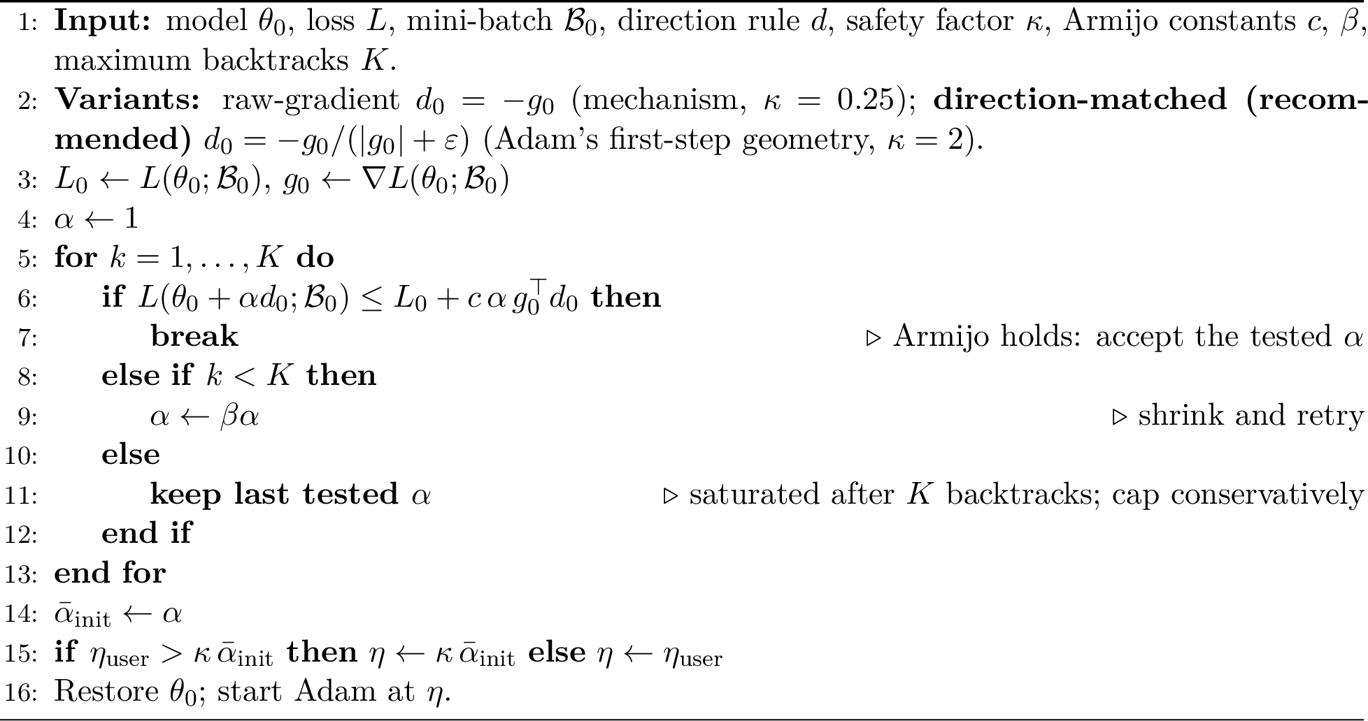
The default value of the safety constant on CIFAR-10/ResNet-18 is \(\kappa = 0.25\). We arrived at this number directly from the empirical divergence boundary of vanilla Adam reported in Appendix 10: vanilla Adam first diverges at \(\eta \approx 0.6\,\bar\alpha_{\text{init}}\), so a safety factor of \(\kappa = 0.25\) leaves a comfortable margin of roughly \(2\times\) without being overly conservative. The choice is forgiving: a sweep over \(\kappa\) (Appendix 9) shows that any \(\kappa \le 0.25\) keeps the rescue intact on CIFAR-10, with graceful rather than catastrophic degradation beyond. For the raw-gradient probe, as Section [sec:results-fashion] will show, \(\kappa\) is architecture-specific and a \(\sim\)one-minute divergence sweep is the recommended way to set it on a new architecture (once chosen it can be reused across hyperparameter searches and seeds); the direction-matched variant introduced next removes this dependence and uses a single fixed \(\kappa = 2\) throughout.
Direction-matched Adam probe. The probe so far line-searches along \(d_0 = -g_0\), but Adam does not step along the raw gradient. Its first update direction is \(-m_0/(\sqrt{v_0}+\varepsilon)\); with bias correction at \(t=1\) this is \(\hat{m}_0 = g_0\) and \(\hat{v}_0 = g_0^2\), so Adam’s first step points along \[d_{\text{Adam}} \;=\; -\,\frac{g_0}{\sqrt{g_0^2}+\varepsilon} \;=\; -\,\frac{g_0}{|g_0|+\varepsilon} \;\approx\; -\operatorname{sign}(g_0),\] the preconditioned direction in which the optimiser actually moves. The direction-matched variant of the probe runs the same backtracking search along \(d_{\text{Adam}}\) instead of \(-g_0\), accepting the largest \(\alpha\in(0,1]\) that satisfies the general Armijo condition \(L(\theta_0 + \alpha\, d_{\text{Adam}};\mathcal{B}_0) \le L_0 + c\,\alpha\, g_0^\top d_{\text{Adam}}\) (note \(g_0^\top d_{\text{Adam}} < 0\)), and caps the learning rate at \(\eta \le \kappa\,\bar\alpha_{\text{Adam}}\) exactly as in Algorithm 1. Because \(\bar\alpha_{\text{Adam}}\) is now measured in Adam’s own geometry, the conversion factor \(\kappa\) no longer has to absorb the per-architecture gradient scale: a single fixed value transfers across architectures, which we establish empirically in Section [sec:results-fashion] (Table 9). This is the variant we recommend when a per-architecture divergence sweep is undesirable; the raw-gradient probe is retained in the body experiments because it admits the clean link to \(\lambda_1\) used to expose the mechanism.
The init probe handles the most common failure mode, a single catastrophically wrong initial learning rate, but cannot react to sharpness changes during training. For users who want continuous in-training adaptation, we provide two periodic controllers that re-run the same Armijo probe every \(K_{\text{probe}}\) Adam steps (default \(K_{\text{probe}} = 50\)) and adjust \(\eta\) from the resulting \(\alpha_t\). The defensive Watchdog maintains a baseline \(\bar\alpha_{\text{base}}\) from the first probe and shrinks \(\eta\) by a factor of two whenever \(\alpha_t / \bar\alpha_{\text{base}}\) falls below \(0.5\); symmetrically it grows \(\eta\) by a factor of \(1.2\) when the ratio recovers above \(0.8\), but never beyond the user’s initial value or below \(0.05\,\eta_{\text{init}}\). The active Tracker simply chases the probed step via an exponential moving average, \(\eta_{t+1} = (1-\beta)\eta_t + \beta\kappa\alpha_t\), with the same \(\kappa\) as the init probe and \(\beta = 0.1\). Both controllers were tuned by inspection on CIFAR-10/ResNet-18; we will see in Section [sec:results-fashion] that their tuned thresholds do not transfer to a small CNN, and that on Fashion-MNIST it is in fact best to disable them and rely on the init probe alone.
As for compute, an init probe consumes one extra forward-and-backward pass at \(\theta_0\) (to obtain the descent direction) plus on average five forward-only backtracking evaluations, in total \(\sim 50\) ms on a single RTX 6000. Because Adam-InitOnly fires this probe only once, its wall-clock overhead is about \(1\%\) on CIFAR-10/ResNet-18, within measurement noise of vanilla Adam. A periodic probe is structurally identical; with the default \(K_{\text{probe}}=50\) the periodic-probe controllers add a measured \(\approx\!2.7\%\) (Adam-Tracker) to \(\approx\!5.3\%\) (Adam-Watchdog) of wall-clock (Section [sec:results-cost]). Evaluating the backtracking trials forward-only, rather than recomputing a gradient at every trial, roughly halves this periodic overhead.
4 Experimental setup↩︎
Our primary testbed is ResNet-18 with the standard CIFAR adaptation (\(3\times 3\) stride-1 conv stem, no max-pool, no pre-trained weights), trained on CIFAR-10 (50k train / 10k test) with standard augmentation (random
crop with 4-pixel padding, horizontal flip), batch size 256, for 10 epochs. On this testbed we benchmark five optimisers, all built on top of the same vanilla Adam implementation (torch.optim.Adam with \(\beta_1=0.9\), \(\beta_2=0.999\), \(\varepsilon=10^{-8}\)). Three are our own contributions of varying complexity: Adam-InitOnly, which performs only
the init probe of Section 3 and then leaves Adam alone; Adam-Watchdog, which additionally re-probes every fifty Adam steps and applies the defensive shrink/grow rule; and Adam-Tracker, which uses the same
periodic probe but feeds it into the active EMA controller. Two are simple and widely deployed baselines that target similar failure modes: Adam + grad-clip, which clips the global gradient norm to one before each Adam update, and Adam +
linear warmup, which initialises Adam at \(\eta_{\text{init}}/100\) and ramps the learning rate linearly to \(\eta_{\text{init}}\) over the first 200 steps. Two recent parameter-free
optimisers, Schedule-Free AdamW [10] and Prodigy [8], complete the comparison in the rescue experiments. Adam-InitOnly uses the raw-gradient probe with a per-architecture \(\kappa\) unless marked “dir.”,
which denotes the direction-matched probe of Algorithm 1 at the fixed \(\kappa = 2\).
Transfer beyond this primary setting is tested on three further benchmarks. Fashion-MNIST (60k train / 10k test) is trained with a small CNN (two convolutional and two fully-connected layers, 0.4M parameters); AG News topic classification (4 classes, 120k/7.6k train/test) with a small from-scratch encoder-only Transformer (4 layers, \(d_{\text{model}} = 128\), word-level tokeniser); and Imagenette [25], the fastai ImageNet subset (10 classes, 9.5k/3.9k train/val images), trained at \(128 \times 128\) with the standard full-stem ResNet-18 as a real-resolution control (Appendix 13). Probe and controllers are identical across all four testbeds; only the data loader and model differ. The Fashion-MNIST CNN also serves as the second architecture in the mechanism experiments below, and the cross-architecture study of the direction-matched probe widens the set to nine models (normalisation variants, an MLP, an LSTM, and Transformers of several scales), introduced where they appear.
Each (optimiser, initial learning rate) combination is run with 5 seeds; we report mean \(\pm\) standard deviation and divergence rate. In the optimiser-comparison tables, bold marks the best mean per column within each
block of rows, since the blocks compare different regimes (standard baselines, probe controllers, parameter-free optimisers; uncalibrated versus calibrated); divergent, partially divergent and chance-level entries are not marked. A run is marked
diverged if loss exceeds \(5\times\) initial or becomes NaN. The mini-batch loss is logged before each update, so the blow-up caused by the destabilising first update is recorded at the next
logged step; throughout, “diverges in the first step” refers to this first update, which our logs flag within the first two logged steps. Hardware: single NVIDIA RTX 6000 Ada Generation per run. The experimental protocol (seeds, averaging, and how the
overhead and curvature numbers were obtained) is detailed in Appendix 14.
5 Results↩︎
We open with the measurement at the heart of the method: what the line-search step reveals about the local loss landscape, and at what cost. The init probe and the periodic probes both estimate, at very low cost, the largest gradient step that the local loss landscape can absorb. We make this connection precise, and we do it for a general descent direction \(d\) (with \(g^\top d < 0\)), because the direction along which the optimiser steps will matter below. On a quadratic loss \(L(\theta) = \tfrac12 (\theta - \theta^\star)^\top H (\theta - \theta^\star)\) with \(H \succ 0\), exact line search along \(d\) chooses the minimiser \[\alpha^\star \;=\; \frac{-\,g^\top d}{d^\top H d} \;=\; \frac{1}{q_d}, \qquad q_d \;:=\; \frac{d^\top H d}{-\,g^\top d},\] where \(q_d\) is the curvature along \(d\). For the raw gradient \(d = -g\) this is \(q_{-g} = g^\top H g / \|g\|^2 \in [\lambda_n, \lambda_1]\), so \(1/\lambda_1 \le \alpha^\star \le 1/\lambda_n\). Empirically we measure \(\alpha\) and the top Hessian eigenvalue \(\lambda_1\) throughout training of ResNet-18 on CIFAR-10 and, as cross-architecture checks, of a plain CNN on Fashion-MNIST and of the standard full-stem ResNet-18 on Imagenette at \(128\)px. The results are reported in Table 1.
| Variant | \(\bar{r}_{\log\alpha,\log\lambda_1}\) | \(\bar{r}_{\text{Spearman}}\) | \(\bar{p}\) | \(\bar\alpha\) |
|---|---|---|---|---|
| Pure Armijo, CIFAR-10/ResNet-18 (3 seeds) | \(-0.913 \pm 0.013\) | \(-0.83 \pm 0.04\) | \(< 10^{-7}\) | \(0.666\) |
| Pure Armijo, Fashion-MNIST/CNN (3 seeds) | \(-0.950 \pm 0.017\) | \(-0.89 \pm 0.04\) | \(< 10^{-10}\) | \(0.292\) |
| Pure Armijo, Imagenette/ResNet-18 (3 seeds) | \(-0.907 \pm 0.021\) | \(-0.85 \pm 0.03\) | \(< 10^{-8}\) | \(0.274\) |
| Pure Armijo, Digits/MLP (1 seed) | \(-0.775\) | \(-0.61\) | \(0.024\) | \(0.95\) |
| GS+Armijo, CIFAR-10/ResNet-18 (1 seed, Appendix) | \(-0.32\) | \(-0.17\) | \(0.18\) (n.s.) | \(0.05\) |
The empirical correlation is strong, reproducible across seeds, and highly significant. Crucially it holds beyond the primary testbed: on Fashion-MNIST with a plain CNN (no residual connections) the log–log Pearson coefficient is \(-0.950 \pm 0.017\), an equally strong relationship to the \(-0.913 \pm 0.013\) measured on CIFAR-10/ResNet-18, and on Imagenette at real resolution it is \(-0.907 \pm 0.021\) with the standard full-stem ResNet-18, so the relation is neither an artefact of one network family nor of thumbnail-resolution inputs. This is the textbook quadratic relation \(\alpha \approx 1/\lambda\) surviving into the deep-net regime in the sense made precise by Edge of Stability [12]: the line search is, in effect, a continuous online estimator of the same \(\lambda_1\) that the EoS literature measures via expensive Lanczos iteration [23].
What does the line search actually invert? The correlation with \(\lambda_1\) combines two facts: an exact, elementary one about backtracking, and a separate alignment fact borrowed from the Edge-of-Stability literature. Separating them shows what is ours and what is not. On a local quadratic model with Hessian \(H \succ 0\), the backtracking line search along any descent direction \(d\) accepts a step \(\alpha\) when \(L(\theta + \alpha d) \le L(\theta) + c\,\alpha\,g^\top d\); expanding \(L\) to second order, this reduces to \(\alpha \le 2(1-c)/q_d\) with the directional curvature \[q_d \;=\; \frac{d^\top H d}{-\,g^\top d}\] introduced above. Backtracking from \(\alpha_{\max}=1\) by factor \(\beta\) accepts the largest such \(\beta^k\), so whenever the constraint binds the returned step obeys \[\frac{q_d}{2(1-c)} \;\le\; \frac{1}{\alpha} \;\le\; \frac{q_d}{2\beta(1-c)} .\] That is, the line search inverts the directional curvature \(q_d\) along the probed direction, not \(\lambda_1\), up to the multiplicative backtracking band of width \(1/\beta\). This exact statement is the part of the mechanism that is ours; which curvature it reports is then entirely a matter of which direction \(d\) one probes, and two choices matter.
The first is the raw-gradient probe, \(d=-g\), for which \(q_{-g} = g^\top H g/\|g\|^2\) is the Rayleigh quotient of \(H\) along the gradient; we write \(q\) for \(q_{-g}\) in the measurement experiments that follow. This is the variant we use to expose the mechanism, because it admits a clean link to the top eigenvalue. We test the band directly by measuring \(\alpha\) and \(q_{-g}\) on the same probe batch at each probe (a single extra Hessian-vector product). Across the CIFAR-10 and Fashion-MNIST mechanism runs, \(73\%\) of the probe points at which the Armijo constraint is active fall inside the predicted factor-\(2\) band, with median ratio \((1/\alpha)/(q_{-g}/(2(1-c))) = 1.27\), comfortably inside the predicted \([1, 1/\beta] = [1, 2]\). The remaining \(\approx 27\%\) sit just outside the band because \(\alpha\) is quantised to powers of \(\beta\) and the mini-batch loss is only locally quadratic. The link to \(\lambda_1\) is then the second, EoS-side fact: we measure \(q_{-g} \approx 0.63\,\lambda_1\) (median over both architectures), i.e.the gradient carries a large but incomplete component along the top eigenvector, so \(1/\alpha \approx q_{-g}/2 \approx 0.3\,\lambda_1\), a strong linear relation with a constant offset, exactly the parallel-but-below line seen in Figure 2. The novel, exact part of the mechanism is \(1/\alpha \propto q_{-g}\); the proportionality \(q_{-g} \propto \lambda_1\) is inherited from the Edge-of-Stability alignment phenomenon [12], [14].
The second choice is the one that makes the probe deployable. Adam does not step along \(-g\); it steps along the preconditioned direction \(d = -g/(\sqrt{v}+\epsilon) \approx -\operatorname{sign}(g)\). Probing along that direction measures \(q_d\) in the geometry the optimiser actually moves in: the curvature that matters is the curvature along the direction the optimiser actually takes. The payoff is concrete: the raw-gradient probe reports curvature in a coordinate system Adam never uses, so the safety factor that converts a probe reading into a step cap is architecture-specific, whereas the Adam-direction probe yields a single safety factor that transfers across networks unchanged. We establish this next, and it is what lets one probe-derived rule guard Adam across all the architectures we test.
Figure 2 visualises this within each architecture: \(1/\alpha\) plotted against \(\lambda_1\) on log–log scales follows a strong linear trend with fitted slopes of order one (\(1.46\) on CIFAR-10, \(1.06\) on Fashion-MNIST, \(1.02\) on Imagenette), lying a roughly constant factor below the textbook \(1/\alpha = \lambda_1\) reference, consistent with the \(1/\alpha \approx 0.3\,\lambda_1\) estimate, a unit-slope law with a constant offset that the fitted slopes bracket (close on Fashion-MNIST, somewhat steeper on CIFAR-10).

The correlation above is a static snapshot; in practice the probe is useful because it tracks sharpness online. Figure 3 overlays, against the training step, the expensive top eigenvalue \(\lambda_1\) (Lanczos), the directional curvature \(q\), and the low-cost probe reading \(1/\alpha\), for one run per architecture. The probe follows \(\lambda_1\) throughout training (here a steady flattening, as the line search drives the iterate into lower-curvature regions) for about five forward passes per reading, against the \(k\) Hessian–vector products (each roughly two backward passes) that a Lanczos estimate of \(\lambda_1\) needs. The reading has a floor: once the landscape is flat enough that the full step \(\alpha = \alpha_{\max} = 1\) is accepted, \(1/\alpha\) saturates at \(1\) and no longer resolves curvature below that level (visible on CIFAR-10 after \(\sim\)1000 steps). Where the Armijo constraint is active, though, the line-search step is a low-cost online sensor for local sharpness: a practical way to watch Edge-of-Stability dynamics without Hessian machinery.

How faithfully does the step read curvature, and what controls the fidelity? Table 2 characterises the probe as a sensor on the Fashion-MNIST CNN, where \(\lambda_1\) is cheap and reliable to estimate (PyHessian/Lanczos) as a reference. Two knobs matter. The backtracking factor \(\beta\) sets the resolution: theory places \(1/\alpha\) in \([q/2(1-c),\, q/2\beta(1-c)]\), a band of width \(1/\beta\), and with the backtracking depth held fixed the reading tightens exactly as predicted, from a median \((1/\alpha)/(q/2)\) of \(1.8\) inside \([1,2]\) at the default \(\beta = 0.5\) to \(1.07\) inside \([1,1.11]\) at \(\beta = 0.9\), at the cost of proportionally more evaluations. The probe batch sets the noise: the relative standard deviation of the \(\lambda_1\) and \(q\) estimates over independent batches falls from \(\approx 0.4\) at batch \(64\) to \(\approx 0.1\) at batch \(256\), so a few hundred examples already give a stable reading. Across these settings the directional curvature is a roughly constant fraction of the top eigenvalue, \(q/\lambda_1 \approx 0.6\), matching the alignment used above.
| backtracking factor \(\beta\) | predicted band \([1,1/\beta]\) | median \((1/\alpha)/(q/2)\) (% in band) |
|---|---|---|
| \(0.5\) (default) | \([1,\,2.00]\) | \(1.79\) (86%) |
| \(0.7\) | \([1,\,1.43]\) | \(1.23\) (86%) |
| \(0.9\) | \([1,\,1.11]\) | \(1.07\) (100%) |
This establishes the paper’s measurement claim: the line search reads local sharpness at low cost. We now turn to the practical pay-off: using that reading, once at initialisation, to cap a mis-specified learning rate. Table 3 reports test accuracy across the full lr range \(\{10^{-3}, 10^{-2}, 10^{-1}, 0.3, 1.0, 3.0\}\) for vanilla Adam and the controllers, mean \(\pm\) std over 5 seeds.
| \(\eta_{\text{init}}\) | \(10^{-3}\) | \(10^{-2}\) | \(10^{-1}\) | \(0.3\) | \(1.0\) | \(3.0\) |
|---|---|---|---|---|---|---|
| Vanilla Adam | \(\mathbf{0.834 \pm 0.025}\) | \(0.811 \pm 0.016\) | DIV. | DIV. | DIV. | DIV. |
| Adam-InitOnly | \(0.833 \pm 0.023\) | \(0.806 \pm 0.016\) | \(\mathbf{0.807 \pm 0.023}\) | \(\mathbf{0.799 \pm 0.026}\) | \(\mathbf{0.794 \pm 0.038}\) | \(\mathbf{0.796 \pm 0.023}\) |
| Adam-Watchdog | \(0.808 \pm 0.051\) | \(\mathbf{0.816 \pm 0.020}\) | \(0.797 \pm 0.010\) | \(0.757 \pm 0.010\) | 0.233 (2/5 div.) | 0.421 (3/5 div.) |
| Adam-Tracker | \(0.803 \pm 0.023\) | \(0.766 \pm 0.022\) | \(0.756 \pm 0.027\) | \(0.765 \pm 0.020\) | \(0.761 \pm 0.026\) | \(0.772 \pm 0.019\) |
| Direction-matched probe, fixed \(\kappa = 2\) (no calibration) | ||||||
| Adam-InitOnly (dir.) | \(\mathbf{0.839 \pm 0.025}\) | \(\mathbf{0.823 \pm 0.016}\) | \(\mathbf{0.828 \pm 0.018}\) | \(\mathbf{0.824 \pm 0.024}\) | \(\mathbf{0.817 \pm 0.020}\) | \(\mathbf{0.823 \pm 0.023}\) |
| Transfer check: AdamW base optimiser | ||||||
| Vanilla AdamW | \(\mathbf{0.843 \pm 0.014}\) | \(0.809 \pm 0.023\) | DIV. | DIV. | DIV. | DIV. |
| AdamW-InitOnly (dir.) | \(0.828 \pm 0.029\) | \(\mathbf{0.823 \pm 0.016}\) | \(\mathbf{0.827 \pm 0.019}\) | \(\mathbf{0.816 \pm 0.018}\) | \(\mathbf{0.818 \pm 0.019}\) | \(\mathbf{0.826 \pm 0.020}\) |
| Parameter-free / schedule-free baselines (no \(\kappa\); \(\eta\) swept like the rest) | ||||||
| Schedule-Free AdamW | \(\mathbf{0.865 \pm 0.005}\) | \(\mathbf{0.864 \pm 0.006}\) | DIV. | DIV. | DIV. | DIV. |
| Prodigy | \(0.100 \pm 0.005\) | \(0.529 \pm 0.003\) | \(\mathbf{0.768 \pm 0.006}\) | \(\mathbf{0.795 \pm 0.011}\) | \(\mathbf{0.813 \pm 0.010}\) | \(\mathbf{0.827 \pm 0.018}\) |

Vanilla Adam is competitive at the optimal \(\eta = 10^{-3}\) (\(0.834\)) but diverges in the very first step at any \(\eta \ge 10^{-1}\); the watchdog absorbs one further decade of misspecification before failing, and the tracker survives the whole range at a persistent accuracy cost (Figure 4). The most informative row is the simplest one. Adam-InitOnly, which performs only the calibration probe before the first Adam step and then leaves Adam entirely alone, matches vanilla Adam at the optimal \(\eta\) (\(0.833\) vs \(0.834\), within seed noise) and stays in \([0.79, 0.83]\) across the full range. It matches or exceeds Adam-Tracker at every learning rate, has no periodic compute overhead, and, as the transfer experiments below show, is the only controller whose settings carry over to other architectures. We recommend Adam-InitOnly as the practical default.
The fair comparison is not vanilla Adam at an arbitrary learning rate (which no practitioner would deliberately choose) but vanilla Adam whose \(\eta\) has been tuned, typically by a learning-rate sweep or range test [5]. Adam-InitOnly delivers essentially that tuned accuracy without the search: its worst cell over the entire range (\(0.794\) at \(\eta = 1.0\)) is within five percent of optimally-tuned vanilla Adam’s best (\(0.834\) at \(\eta = 10^{-3}\)), and it reaches this from a single probe at every learning rate. We make this comparison concrete in Table 4: against an actual learning-rate range test [5] that ramps \(\eta\) over \(\sim\!2\) epochs and then trains at the rate it finds, the one-shot probe (given a deliberately too-large \(\eta = 0.1\) to cap) reaches the same or slightly better test accuracy (\(0.822\) vs \(0.792\), 3 seeds, both with zero divergences) for the cost of a single \(\sim\!50\) ms probe rather than the range test’s \(\sim\!2\) ramp epochs. The probe is therefore best read not as beating a deliberately broken baseline, but as approximating the safety role of a coarse learning-rate sweep at a fraction of its cost. The probe targets the safety role of a range test rather than the search for a performance-optimal rate, and it occupies that role for the cost of one probe.
| Method | effective \(\eta\) | test acc | extra cost | div. |
|---|---|---|---|---|
| LR range test (Smith) \(\to\) train | \(0.018\) | \(0.792\) | \(\sim\!2\) epochs (ramp) | \(0/3\) |
| Adam-InitOnly (probe @ \(\eta = 0.1\)) | \(0.016\) | \(\mathbf{0.822}\) | \(\sim\!1\) probe (\(\sim\!50\) ms) | \(0/3\) |
Modern parameter-free optimisers do not remove the need for this safeguard. The last two rows of Table 3 report two recent parameter-free / schedule-free optimisers run across the same grid: Schedule-Free AdamW [10] and Prodigy [8].1 Neither covers the full range. Schedule-Free AdamW is strongest of all at small \(\eta\) (\(0.865\)/\(0.864\) at \(\eta \le 10^{-2}\), above every other method) but still diverges in the first step for any \(\eta \ge 10^{-1}\), exactly the failure our probe targets. Prodigy never diverges, but its internal step-size estimate starts far too small at \(\eta = 10^{-3}\) (test accuracy at random-guess level) and only becomes competitive once \(\eta \ge 10^{-1}\), where it is in fact the best method (\(0.813\)/\(0.827\) at \(\eta = 1.0\)/\(3.0\)). Each parameter-free optimiser thus excels in a different part of the range but collapses at the opposite end, whereas Adam-InitOnly stays within about four percentage points of its own optimum across the entire \(10^{-3}\)–\(3.0\) range with no divergence; the probe is a calibrate-once safety check for Adam, not a competing optimiser, and these results are complementary rather than contradictory.
The direction-matched block of Table 3 removes even the one-time calibration: at the single fixed \(\kappa = 2\), the direction-matched probe matches the calibrated raw-gradient variant across the entire grid (\(0.82\)–\(0.84\), zero divergences), with no per-architecture sweep at all. The AdamW block repeats the experiment with the base optimiser swapped: vanilla AdamW diverges from \(\eta = 0.1\) exactly like Adam, and the identical probe at the identical \(\kappa\) restores the full range.
Figure 5 shows the \(\eta = 10^{-1}\) case explicitly: vanilla Adam’s loss explodes within two steps and is irrecoverable, while Adam-InitOnly and the two periodic controllers all train normally. Figure 6 shows what the controllers actually do with \(\eta\): the rescue is done up front by the init probe, which caps the requested \(\eta = 0.1\) down to \(\approx 0.016\) before the first update. From there the two periodic controllers relax the rate rather than throttle it further: the watchdog climbs back to the user’s \(0.1\) ceiling and holds, while the tracker follows the probed step size up to \(\approx 0.25\). The rescue is therefore attributable to the one-shot cap, not to continued shrinking during training, which is precisely why the init probe alone suffices.


A reasonable concern is that the rescue effect is also achieved by simpler standard tricks. Table 5 compares the controllers against gradient norm clipping (\(\|g\| \le 1.0\)) and a 200-step linear warmup at the two diagnostic learning rates \(\eta = 10^{-1}\) and \(\eta = 1.0\).
| \(\eta_{\text{init}} = 10^{-3}\) | \(\eta_{\text{init}} = 10^{-1}\) | \(\eta_{\text{init}} = 1.0\) | |
|---|---|---|---|
| Vanilla Adam and standard defences | |||
| Vanilla Adam | \(0.834 \pm 0.025\) | DIV. | DIV. |
| Adam + grad-clip (\(\|g\| \le 1\)) | \(\mathbf{0.836 \pm 0.021}\) | DIV. | DIV. |
| Adam + 200-step warmup | \(0.835 \pm 0.015\) | \(\mathbf{0.809 \pm 0.028}\) | \(0.10\)* (3/5 div.) |
| Probe-based controllers (ours) | |||
| Adam-InitOnly | \(\mathbf{0.833 \pm 0.023}\) | \(\mathbf{0.807 \pm 0.023}\) | \(\mathbf{0.794 \pm 0.038}\) |
| Adam-Watchdog | \(0.808 \pm 0.051\) | \(0.797 \pm 0.010\) | \(0.233\) (2/5 div.) |
| Adam-Tracker | \(0.803 \pm 0.023\) | \(0.756 \pm 0.027\) | \(0.761 \pm 0.026\) |
* Surviving seeds failed to learn; test accuracy at random-guess level.
The two low-cost baselines are revealing in different ways. Global gradient-norm clipping at \(\|g\|\le 1\) leaves vanilla Adam essentially unchanged at well-tuned learning rates (\(0.836 \pm 0.021\) at \(\eta = 10^{-3}\) against vanilla Adam’s \(0.834 \pm 0.025\), identical within seed noise), so the clip neither helps nor hurts there. At misspecified learning rates it provides no rescue at all: Adam still diverges in the first step at \(\eta = 10^{-1}\) and at \(\eta = 1.0\). The reason is structural rather than numerical. Adam’s update is \(\eta\, m_t/(\sqrt{v_t} + \varepsilon)\), and during the first few steps \(v_t\) is initialised at zero and the \(1/\sqrt{v_t}\) factor amplifies even a clipped gradient by orders of magnitude; clipping the gradient before this amplification has limited effect on the resulting parameter update. Linear warmup performs better but only partially: it absorbs \(\eta = 10^{-1}\) at accuracy on par with the init probe (\(0.809 \pm 0.028\) vs \(0.807 \pm 0.023\)), but at \(\eta = 1.0\) the warmup target is itself unstable, with three of five seeds diverging and the surviving seeds settling at the random-guess level. Of the probe-based controllers, both Adam-InitOnly and Adam-Tracker survive every tested learning rate up to \(\eta = 3.0\) (Table 3), whereas Adam-Watchdog fails from \(\eta = 1.0\) on; Adam-InitOnly does so at the higher accuracy and, as we show next, is the only one whose single setting also transfers to a second architecture.
A single architecture is not enough to trust the recipe, so we now ask whether the controller settings transfer. To test this, we ran the same sweep on the Fashion-MNIST CNN, with the same default \(\kappa = 0.25\) and watchdog thresholds calibrated on CIFAR-10. Five seeds per cell. The result is reported in the upper block of Table 6, alongside the calibrated version discussed below.
Inspecting the controller logs reveals two distinct failures: (i) On Fashion-MNIST the probe saturates: the Armijo condition already holds at the full step, so \(\bar\alpha_{\text{init}} = 1\), unlike on CIFAR-10, where backtracking engages and returns \(\bar\alpha_{\text{init}} \approx 0.06\). At the same time the largest stable Adam learning rate on Fashion-MNIST/small-CNN is only \(\approx 0.01\) (cf.vanilla Adam’s divergence at \(\eta = 0.1\)), so the stable fraction of the probed step is \(\approx 0.01\) here against \(\approx 0.3\) on CIFAR-10; the conversion factor \(\kappa\) must therefore absorb a gap of well over an order of magnitude. The default safety factor \(\kappa = 0.25\) caps \(\eta\) at \(0.25\), far above the stable range: at \(\eta = 0.1\) the cap does not engage at all, and at the larger requested rates it does engage but only reduces them to \(0.25\), which is itself still unstable, so the init-probe rescue cannot help here. (ii) On the small CNN, sharpness rises much faster in the first hundred steps (progressive sharpening is more violent on a small network), so \(\alpha\) collapses from \(1\) to \(\approx 0.008\) within 100 steps. Watchdog interprets this as a divergence signal and shrinks \(\eta\) from \(0.001\) to its floor \(5\times 10^{-5}\), well below the optimum.
The fix follows directly from this diagnosis, and it makes the recipe simpler rather than more complex. We re-ran the same Fashion-MNIST sweep with \(\kappa\) recalibrated to the architecture: the largest stable vanilla-Adam learning rate is \(\approx 10^{-2}\) (cf.the upper block of Table 6), and \(\bar\alpha_{\text{init}} \approx 1\), so we pick \(\kappa = 0.005\) (half of the empirical stability boundary).
| \(\eta_{\text{init}}\) | \(10^{-3}\) | \(10^{-2}\) | \(10^{-1}\) | \(0.3\) | \(1.0\) | \(3.0\) |
|---|---|---|---|---|---|---|
| Uncalibrated, \(\kappa = 0.25\) (CIFAR-10 default) | ||||||
| Vanilla Adam | \(0.916 \pm 0.003\) | \(0.890 \pm 0.008\) | DIV. | DIV. | DIV. | DIV. |
| Adam + grad-clip | \(\mathbf{0.917 \pm 0.002}\) | \(0.899 \pm 0.004\) | DIV. | DIV. | DIV. | DIV. |
| Adam + warmup | \(0.913 \pm 0.004\) | \(\mathbf{0.903 \pm 0.003}\) | DIV. | 0.10\(^*\) (2/5) | 0.10\(^*\) | DIV. |
| Adam-Watchdog | \(0.878 \pm 0.002\) | \(0.889 \pm 0.013\) | DIV. | DIV. | DIV. | DIV. |
| Adam-Tracker | 0.81 (3/5) | 0.10\(^*\) (4/5) | DIV. | DIV. | DIV. | DIV. |
| Calibrated, \(\kappa = 0.005\) (one extra divergence sweep, \(<\!1\) minute) | ||||||
| Adam-InitOnly | \(\mathbf{0.914 \pm 0.005}\) | \(\mathbf{0.909 \pm 0.004}\) | \(\mathbf{0.909 \pm 0.004}\) | \(\mathbf{0.909 \pm 0.004}\) | \(\mathbf{0.908 \pm 0.003}\) | \(\mathbf{0.907 \pm 0.003}\) |
| Adam-Watchdog | \(0.878 \pm 0.002\) | \(\mathbf{0.909 \pm 0.005}\) | \(\mathbf{0.909 \pm 0.004}\) | \(0.895 \pm 0.004\) | 0.65 (1/5) | 0.10\(^*\) (4/5) |
| Adam-Tracker | DIV. | 0.46 (3/5) | 0.10\(^*\) (4/5) | 0.84 (4/5) | 0.10\(^*\) (3/5) | DIV. |
| Direction-matched probe, fixed \(\kappa = 2\) (no calibration) | ||||||
| Adam-InitOnly (dir.) | \(\mathbf{0.914 \pm 0.004}\) | \(\mathbf{0.900 \pm 0.005}\) | \(\mathbf{0.896 \pm 0.015}\) | \(\mathbf{0.899 \pm 0.014}\) | \(\mathbf{0.897 \pm 0.012}\) | \(\mathbf{0.898 \pm 0.010}\) |
| Parameter-free / schedule-free baselines (no \(\kappa\)) | ||||||
| Schedule-Free AdamW | \(\mathbf{0.914 \pm 0.001}\) | \(\mathbf{0.920 \pm 0.002}\) | DIV. | DIV. | DIV. | DIV. |
| Prodigy | \(0.102 \pm 0.046\) | \(0.876 \pm 0.002\) | \(\mathbf{0.915 \pm 0.004}\) | \(\mathbf{0.917 \pm 0.002}\) | \(\mathbf{0.911 \pm 0.006}\) | \(\mathbf{0.910 \pm 0.009}\) |
2pt
The result is unambiguous: with one-time calibration of \(\kappa\), Adam-InitOnly yields test accuracy \(0.91 \pm 0.005\) across all six learning rates, 5 seeds each, with zero divergences. This mirrors and even strengthens the CIFAR-10 rescue result: across more than three orders of magnitude of misspecification (\(10^{-3}\) to \(3.0\)), test accuracy drops by less than 1 percentage point relative to the optimal vanilla-Adam configuration. The direction-matched probe achieves the same without the sweep (final block; Figure 4, bottom left): \(0.90\)–\(0.91\) across all six rates, zero divergences, at the fixed \(\kappa = 2\). The two parameter-free baselines (last block of Table 6) again cover only part of the range: Schedule-Free AdamW is the strongest method at \(\eta \le 10^{-2}\) but diverges for \(\eta \ge 10^{-1}\), while Prodigy is robust from \(10^{-2}\) to \(3.0\) yet collapses to random-guess accuracy at \(\eta = 10^{-3}\). The two failure modes are complementary and opposite, and neither matches the calibrated init probe’s coverage of all six rates.
The simpler controller wins here for a structural reason. The Watchdog and Tracker modes were tuned on CIFAR-10/ResNet-18, where progressive sharpening [12] is comparatively gentle and the periodic adjustments tracked the curvature dynamics usefully. On a small CNN with stronger progressive sharpening, the same periodic adjustments overshoot: the Watchdog shrinks \(\eta\) down to its floor of \(0.05\,\eta_{\text{init}}\), the Tracker EMA pulls \(\eta\) outside the stable range. Removing the periodic component (Adam-InitOnly) lets Adam’s own adaptive \(1/\sqrt{v_t}\) scaling handle in-training curvature changes, and performs strictly better. This sharpens the recommendation: the init probe is the primary mechanism, and periodic probing is at most a safety net that requires its own per-architecture tuning.
This calibration is low-cost. The extra cost of fixing \(\kappa\) to a new architecture is a single divergence sweep like the one in Appendix 10 (\(\sim 50\) Adam runs of \(\le 1\) epoch each), or roughly one minute on the hardware of Section 4. Once calibrated, Adam-InitOnly deploys with \(<\!2\%\) wall-clock overhead per training run.
To test whether the recipe extends beyond vision, we repeat the study on the text benchmark: AG News with the small Transformer. The probe and controllers are unchanged; results over the same \(6\times5\) grid are in Table 7.
| \(\eta_{\text{init}}\) | \(10^{-3}\) | \(10^{-2}\) | \(10^{-1}\) | \(0.3\) | \(1.0\) | \(3.0\) |
|---|---|---|---|---|---|---|
| Uncalibrated, \(\kappa = 0.25\) (CIFAR-10 default) | ||||||
| Vanilla Adam | \(0.902 \pm 0.003\) | \(0.250\) | DIV. | DIV. | DIV. | DIV. |
| Adam-InitOnly | \(\mathbf{0.905 \pm 0.003}\) | \(0.250\) | \(0.250\) | \(0.250\) | \(0.250\) | \(0.250\) |
| Adam-Watchdog | \(0.904 \pm 0.002\) | \(0.250\) | \(0.250\) | DIV. | DIV. | DIV. |
| Adam-Tracker | DIV. | DIV. | DIV. | DIV. | DIV. | DIV. |
| Schedule-Free AdamW | \(0.903 \pm 0.003\) | \(0.251\) | 0.250 (3/5 div.) | DIV. | DIV. | DIV. |
| Prodigy | \(0.232 \pm 0.007\) | \(\mathbf{0.880 \pm 0.002}\) | \(\mathbf{0.906 \pm 0.002}\) | \(\mathbf{0.908 \pm 0.002}\) | \(0.408 \pm 0.195\) | \(0.259 \pm 0.018\) |
| Calibrated, \(\kappa = 0.05\) (one extra divergence sweep, \(<\!1\) minute) | ||||||
| Adam-InitOnly | \(\mathbf{0.905 \pm 0.003}\) | \(\mathbf{0.909 \pm 0.002}\) | \(\mathbf{0.909 \pm 0.002}\) | \(\mathbf{0.909 \pm 0.002}\) | \(\mathbf{0.909 \pm 0.002}\) | \(\mathbf{0.909 \pm 0.002}\) |
| Adam-Watchdog | \(0.904 \pm 0.002\) | \(0.250\) | \(0.250\) | DIV. | DIV. | DIV. |
| Adam-Tracker | DIV. | DIV. | DIV. | DIV. | DIV. | DIV. |
| Direction-matched probe, fixed \(\kappa = 2\) (no calibration) | ||||||
| Adam-InitOnly (dir.) | \(\mathbf{0.904 \pm 0.003}\) | \(0.250\) | \(0.250\) | \(0.250\) | \(0.250\) | \(0.250\) |
The pattern mirrors Fashion-MNIST closely. With the CIFAR default \(\kappa = 0.25\), no method is robust: vanilla Adam, Adam-InitOnly and Adam-Watchdog all collapse to random-guess accuracy the moment \(\eta \ge 10^{-2}\), because the largest stable Adam learning rate on this Transformer is only \(\approx 3\times10^{-3}\) and the probe’s safe-step estimate at initialisation (\(\bar\alpha_{\text{init}} \approx 0.031\)) caps \(\eta\) at \(0.25\,\bar\alpha_{\text{init}} \approx 8\times10^{-3}\), still above the stable range. The two parameter-free baselines again cover only part of the grid: Schedule-Free AdamW fails for \(\eta \ge 10^{-2}\), and Prodigy is robust only in a middle band (\(10^{-2}\) to \(0.3\)) while failing at both ends. After the divergence sweep sets \(\kappa = 0.05\), Adam-InitOnly recovers \(0.905\)–\(0.909\) across all six learning rates, more than three orders of magnitude of misspecification, with zero divergences. The periodic controllers do not transfer even after recalibration, confirming that the one-shot init probe, not the periodic machinery, is the component that generalises across domains.
The direction-matched probe marks the limit of the calibration-free recipe here (final block of Table 7; Figure 4, bottom right). At the fixed \(\kappa = 2\) it still prevents every divergence, but on this Transformer, whose stable range is unusually narrow (\(\eta \approx 10^{-3}\)), the uncalibrated cap lands in the stable-yet-unproductive band, and the runs sit at chance for \(\eta \ge 10^{-2}\). Where the stable range is that narrow, the fixed cap is a divergence safeguard only; the calibration sweep is what turns it into a full rescue.
Imagenette, the real-resolution control of Section 4, completes the transfer picture. Vanilla Adam repeats the CIFAR-10 pattern exactly, competitive at \(\eta = 10^{-3}\) and diverging in the first step from \(\eta = 0.1\) on, and the fixed \(\kappa = 2\) again removes every divergence while staying within about five points of the tuned optimum (Figure 4, top right; exact numbers in Appendix 13). The rescue thus carries over from thumbnails to real images and to the unmodified stem.
A sharper test is the case where the default learning rate is itself unsafe. On every benchmark above the Adam framework default \(\eta = 10^{-3}\) lies in the stable range, so the init cap never fires and training is untouched. Its value appears only where the default is genuinely too large for the curvature at initialisation. Two well-known such regimes are normalisation-free networks and warmup-free deep Transformers (Table 8): a ResNet-18 with all normalisation removed on CIFAR-10, and a deeper \(12\)-layer variant of the AG News Transformer (versus the \(4\)-layer model used above) trained without warmup. At the default \(\eta = 10^{-3}\) vanilla Adam diverges (no-normalisation ResNet, all seeds) or collapses to chance (warmup-free Transformer); Adam-InitOnly, with \(\kappa\) recalibrated by the same sweep, caps the rate into the stable range and recovers accuracy within a point or two of the best tuned vanilla Adam, without the user knowing the safe rate in advance. The caveat is that the CIFAR default \(\kappa = 0.25\) does not transfer to these higher-curvature settings (it still diverges). Together with the CIFAR-10 grid, these results establish the paper’s rescue claim: the one-shot cap rescues where the default rate is genuinely unsafe and is a no-op otherwise.
| Setting | vanilla, default \(10^{-3}\) | vanilla, best tuned | Adam-InitOnly @ \(10^{-3}\) |
|---|---|---|---|
| ResNet-18, no normalisation (CIFAR-10) | DIV.(4/4) | \(0.537\) (\(\eta{=}3{\times}10^{-4}\)) | \(0.535\) (\(\kappa{=}0.05\)) |
| Transformer, no warmup (AG News) | \(0.250\) (chance) | \(0.828\) (\(\eta{=}3{\times}10^{-4}\)) | \(0.810\) (\(\kappa{=}0.005\)) |
Two further checks (the empirical divergence boundary that fixes \(\kappa\), and a 100-epoch cosine schedule on which the rescued runs retain their full \(\approx 93\%\) accuracy across the entire grid) are deferred to Appendices 10 and 11.
The rescues above each used a per-architecture \(\kappa\), set by a one-minute divergence sweep, and this is their main practical drawback. It is, however, a property of the probed direction, not of the method, and the direction-matched probe removes it. The plain-gradient probe reports \(\bar\alpha_{\text{init}}\) in a coordinate system Adam never steps in, so the conversion factor that \(\kappa\) must absorb depends on the per-architecture gradient scale. Probing instead along Adam’s own preconditioned direction \(-g/(\sqrt{v}+\varepsilon) \approx -\operatorname{sign}(g)\) returns \(\bar\alpha_{\text{init}}\) in the geometry Adam actually moves in, and that dependence disappears. Table 9 confirms it. A single fixed \(\kappa = 3\), chosen on four architectures and held out on five unseen ones, caps safely across nine architectures (BatchNorm, GroupNorm and normalisation-free nets; a plain MLP; an LSTM; CNNs and Transformers of several scales) and two learning rates: \(2\) divergences in \(54\) runs, against \(10\) for the plain-gradient probe at a single \(\kappa\) and \(22\) for vanilla Adam, and zero at the framework default. Both failures occur on a plain MLP at the \(100\times\)-too-large rate, and a sweep of the safety factor (Table 10) removes them: \(\kappa = 2\) and even \(\kappa = 1\) give zero divergences in all \(54\) runs at no accuracy cost, so we recommend \(\kappa = 2\) as the less intrusive of the two divergence-free settings. Accuracy tells the same story (Table 9, lower block): counting a divergent run as zero, the direction-matched probe reaches a mean of \(0.73/0.63\) at the default/\(100\times\) rate, against \(0.59/0.09\) for vanilla Adam and \(0.55/0.29\) for the plain-gradient probe. Because the nine architectures have different chance levels and task difficulties, Figure 7 breaks the discriminating \(100\times\) rate down per architecture: at \(\kappa = 2\) the direction-matched probe is the most accurate variant on each and diverges on none (exact numbers in Appendix 12). The full learning-rate grids extend this beyond the two spot rates: at the same fixed \(\kappa = 2\) the direction-matched probe diverges nowhere up to \(\eta = 3.0\) on all four benchmarks, with full accuracy recovery on CIFAR-10, Fashion-MNIST and Imagenette (Appendix 13) and the AG News limit discussed above (final blocks of Tables 3, 6 and 7). The same recipe also transfers to AdamW unchanged (AdamW block of Table 3). The per-architecture \(\kappa\) of the body experiments, which predate this fix, is thus a limitation of the gradient-direction probe rather than of the safeguard itself.
| vanilla Adam | plain-grad probe (\(\kappa = 0.25\)) | Adam-direction probe (\(\kappa = 3\)) | |
|---|---|---|---|
| Divergent runs | |||
| at default \(\eta = 10^{-3}\) (of 27) | \(1\) | \(2\) | \(\mathbf{0}\) |
| at \(100\times\) too large (of 27) | \(21\) | \(8\) | \(\mathbf{2}\) |
| total (of 54) | \(22\) | \(10\) | \(\mathbf{2}\) |
| Mean test accuracy (divergent run \(=0\)) | |||
| at default \(\eta = 10^{-3}\) | \(0.586\) | \(0.548\) | \(\mathbf{0.730}\) |
| at \(100\times\) too large | \(0.089\) | \(0.292\) | \(\mathbf{0.631}\) |
| Adam-direction probe | \(\kappa = 1\) | \(\kappa = 2\) | \(\kappa = 3\) |
|---|---|---|---|
| divergences at default \(10^{-3}\) (of 27) | \(\mathbf{0}\) | \(\mathbf{0}\) | \(0\) |
| divergences at \(100\times\) (of 27) | \(\mathbf{0}\) | \(\mathbf{0}\) | \(2\) |
| total divergences (of 54) | \(\mathbf{0}\) | \(\mathbf{0}\) | \(2\) |
| mean acc at default \(10^{-3}\) | \(0.728\) | \(0.703\) | \(0.730\) |
| mean acc at \(100\times\) | \(\mathbf{0.737}\) | \(0.733\) | \(0.631\) |

Finally we turn to cost. Wall-clock overhead in our setting is dominated by the explicit Hessian probes used to measure the \(\alpha\)–\(\lambda_1\) correlation above; the probes are an instrumentation artefact and are not part of the deployed controller. We report the two sets separately. With Hessian probes turned on, vanilla Adam takes 73.1 seconds for ten CIFAR-10 epochs, Adam-Tracker takes 76.1 seconds (+4%), and Adam-Watchdog takes 80.4 seconds (+10%); the difference is the extra forward and forward-backward passes the periodic Armijo probe performs. With Hessian probes turned off (the deployed configuration), the cost depends on how often the controller probes. Adam-InitOnly probes once, at initialisation: one extra forward-and-backward pass plus a handful of forward-only backtracks, an overhead of about \(1\%\) that is within measurement noise of vanilla Adam. The periodic controllers cost more. In a controlled interleaved benchmark (3 seeds, single session, GPU warmed up) over ten CIFAR-10 epochs, vanilla Adam takes \(56.9\) s; Adam-Tracker adds \(+2.7\%\) and Adam-Watchdog \(+5.3\%\). These figures use forward-only backtracking; recomputing a gradient at every backtracking trial (the naive implementation) roughly doubles the periodic overhead, with Adam-Watchdog rising from \(+5.3\%\) to \(+12.0\%\), which is why the probe evaluates the trial loss without a backward pass.
Several limitations bound these claims. The first, the per-architecture \(\kappa\) of the plain-gradient probe, was addressed above: it is a property of the probed direction, and the direction-matched probe removes it.
A second limitation, related to the first, is the fragility of the periodic-probe controllers under rapid progressive sharpening: on the small CNN their pre-tuned thresholds and EMA constants overshoot the true sharpness boundary, and even after \(\kappa\) is recalibrated both underperform Adam-InitOnly. We accordingly keep Watchdog and Tracker as opt-in features for users who want continuous in-training adaptation.
To quantify this, we compared the periodic Tracker across regimes at the framework default \(\eta = 10^{-3}\) (Table 11). On well-conditioned real tasks its step-size growth overshoots and hurts: it loses several accuracy points on CIFAR-10/ResNet-18 and diverges on the AG-News Transformer (\(5/5\) seeds), at every probe interval \(K\) we tried, so the failure is intrinsic to raising the rate on a smooth landscape rather than a matter of tuning \(K\). On a plateau-dominated toy (a \(2\)-\(2\) XOR network, 100 seeds) the Tracker does help, with \(66\%\) of seeds solved versus \(52\%\) at the default, but a fixed higher learning rate (\(\eta = 0.1\)) already solves \(61\%\), so most of the gain is that of an effectively larger step rather than of online adaptivity. We also note that where a task is hard for representational rather than step-size reasons (sharp discontinuities, high-frequency targets), the default rate is already in the stable range and the init cap does not fire; the probe is, by design, silent there. These observations bound the claims to the one-shot init probe, on which the paper rests.
| Regime (default \(\eta = 10^{-3}\)) | vanilla Adam | Watchdog | Tracker |
|---|---|---|---|
| Smooth: CIFAR-10 / ResNet-18 (test acc) | \(0.834\) | \(0.808\) | \(0.803\) |
| Smooth: AG News / Transformer (test acc) | \(0.902\) | \(0.904\) | DIV. |
| Plateau toy: \(2\)-\(2\) XOR (% solved) | \(52\) | \(52\) | \(66\) |
In the same spirit we tested whether the probe could serve as an in-training early-warning signal for instability, rather than a controller. In our tests it did not provide a reliable early-warning signal for runtime divergence, for two reasons we observed across mini-batch (LSTM language modelling on War & Peace, CNNs) and full-batch Edge-of-Stability regimes: the reading does not discriminate (local curvature rises during healthy Edge-of-Stability training as much as before a blow-up), and the divergences we could induce were too abrupt to leave actionable lead time. On the evidence we have, the probe’s value is therefore at initialisation (a curvature sensor and a safety cap), not as a runtime monitor; whether a refined variant could recover a usable signal we leave open.
Finally, the empirical scope of this paper is deliberately narrow. We report controlled experiments on three image-classification benchmarks (CIFAR-10 with a ResNet-18, Fashion-MNIST with a small two-conv CNN, and Imagenette with a standard ResNet-18 at \(128\)px) and one text-classification benchmark (AG News with a small from-scratch Transformer); we do not test the rescue on large language models, on self-supervised vision pre-training, or at ImageNet scale. The empirical link between the line-search step and the top Hessian eigenvalue is established for three architectures, not claimed universal. The Discussion below sketches the experiments that would, in our view, justify a stronger general claim.
6 Discussion↩︎
We have shown that classical Armijo line search, used as a probe rather than as the optimiser, robustifies Adam against a specific but common failure mode: an over-large initial learning rate. Its soundness rests on a clean, empirically reproducible link between the line-search step and the top Hessian eigenvalue.
In our framing, the probe is to Adam what airbags are to a car: a low-cost defence against a specific class of errors that does not change the normal driving experience. It leaves well-tuned training untouched and converts a reliably divergent run into a near-optimal one.
The mechanism is optimiser-agnostic in principle, and a first transfer check supports this: on CIFAR-10/ResNet-18, AdamW [2] diverges for every \(\eta \ge 0.1\) exactly like Adam, and the direction-matched probe at the same fixed \(\kappa = 2\) removes every divergence while holding test accuracy at \(0.82\)–\(0.83\) across the full grid (AdamW block of Table 3). Whether the same holds for optimisers with a different first-step geometry, such as RMSProp [26], we leave open.
The main remaining direction is validation at larger scale: large language models, self-supervised pre-training, or ImageNet-scale training, where both the divergence boundary and the empirical link between the line-search step and the top Hessian eigenvalue may behave differently from the regime studied here. This is beyond our single-GPU budget and we leave it to future work, together with the question of whether the probe-as-controller idea is best combined with, rather than compared against, the parameter-free optimisers (D-Adaptation [7] and Mechanic [9], which we discuss but do not run, would belong in that comparison).
7 Conclusion↩︎
A single Armijo backtracking line search (five forward evaluations and one backward pass) is a low-cost, Hessian-free sensor for local sharpness: the step inverts the directional curvature \(q = g^\top H g/\|g\|^2\) within the derived backtracking band, and \(1/\alpha\) tracks \(\lambda_1\) at Pearson \(-0.91\) to \(-0.95\) across three architectures: the textbook relation \(\alpha^\star \approx 1/\lambda_1\), recovered for the price of a few forward passes rather than Lanczos iteration. The practical pay-off is a one-shot learning-rate cap that keeps Adam within a few points of its tuned accuracy across \(\eta \in [10^{-3}, 3.0]\) on CIFAR-10, Fashion-MNIST, Imagenette and AG News, where vanilla Adam diverges from \(\eta = 0.1\) on. Probing along Adam’s own preconditioned direction makes the safety factor transferable: one fixed \(\kappa = 2\) yields zero divergences on nine architectures and across the full grids of all four benchmarks, recovers full accuracy everywhere except the narrow-stable-range AG News Transformer, carries over to AdamW unchanged, and costs about one percent. We hope the low-cost curvature reading, more than the safeguard itself, encourages the use of line-search quantities as loss-landscape diagnostics.
8 The negative result on the Golden-Section preselection↩︎
This project began as an attempt to build a bounded golden-section plus Armijo line-search optimiser (GGAO); the failure reported here motivated treating the line search as a measurement instead. The bounded golden-section line search on \([0, 1]\) consistently selects very small \(\alpha\) (\(\bar{\alpha} \approx 0.05\) throughout training) and drives the trajectory into regions of high \(\lambda_1\) (\(\bar\lambda_1 \approx 800\)). Pure Armijo on the same architecture and initialisation saturates at \(\alpha = 1\) and stays in low-\(\lambda_1\) regions (\(\bar\lambda_1 \approx 200\)). The \(\alpha\)-\(\lambda_1\) correlation, which is \(-0.91 \pm 0.01\) for pure Armijo on CIFAR-10/ResNet-18, drops to a non-significant \(-0.32\) for GS+Armijo. The golden-section step finds spurious early local minima of the noisy mini-batch loss along the descent direction, where pure backtracking correctly accepts the largest step that satisfies sufficient decrease. We report this negative result here as a warning against bounded non-monotone line searches on stochastic deep-learning losses.
9 Sensitivity to the safety factor \(\kappa\)↩︎
The rescue depends on a single scalar, the safety factor \(\kappa\), which caps the user learning rate at \(\kappa\,\bar\alpha_{\text{init}}\). To quantify how forgiving this choice is, we sweep \(\kappa \in \{0.05, 0.1, 0.25, 0.5, 1.0\}\) for Adam-InitOnly on CIFAR-10/ResNet-18 at three representative learning rates (the optimal \(10^{-3}\), and two values at which vanilla Adam diverges), 3 seeds each. Table 12 reports the result.
| \(\kappa\) | \(\eta=10^{-3}\) | \(\eta=10^{-1}\) | \(\eta=1.0\) |
|---|---|---|---|
| \(0.05\) | \(0.842 \pm 0.007\) | \(\mathbf{0.824 \pm 0.016}\) | \(\mathbf{0.829 \pm 0.019}\) |
| \(0.1\) | \(0.813 \pm 0.026\) | \(0.812 \pm 0.012\) | \(0.813 \pm 0.009\) |
| \(0.25\) | \(0.824 \pm 0.012\) | \(0.794 \pm 0.011\) | \(0.801 \pm 0.020\) |
| \(0.5\) | \(0.836 \pm 0.019\) | \(0.735 \pm 0.033\) | \(0.725 \pm 0.044\) |
| \(1.0\) | \(0.829 \pm 0.021\) | DIV. | DIV. |
At the optimal \(\eta = 10^{-3}\) the cap rarely binds, so accuracy is near-constant across \(\kappa\). At the misspecified rates the trend is monotone: smaller \(\kappa\) caps the learning rate more aggressively and preserves accuracy, whereas \(\kappa = 1.0\) leaves the step essentially uncapped and Adam diverges exactly as in the vanilla baseline. The default \(\kappa = 0.25\) used for CIFAR-10 sits comfortably inside the safe band; the rescue degrades gracefully rather than catastrophically as \(\kappa\) grows, which is why a coarse one-minute calibration suffices.
10 Adam’s divergence threshold and the safety factor \(\kappa\)↩︎
The architecture-independent choice of \(\kappa\) is made from the one-shot probe itself, through the safety sweep of Table 10 (\(\kappa = 2\) for the direction-matched probe, zero divergences across nine architectures). As a complementary check we here locate the absolute divergence boundary of Adam and confirm it sits close to the line-search scale. For this single measurement we anchor to a low-variance estimate \(\bar{\alpha}\) obtained by averaging the Armijo step over a short (200-step) warmup, rather than the raw init value, which is noisier and can saturate at \(\alpha = 1\) on low-curvature initialisations; this gives \(\bar{\alpha} = 0.0393\) on CIFAR-10/ResNet-18. We then trained Adam at \(\eta = m \cdot \bar{\alpha}\) for \(m \in \{0.25, 0.4, 0.5, 0.6, 0.7, 0.8, 0.9, 1.0, 1.5, 2.0, 5.0\}\). Table 13 summarises the result.
| \(m = \eta / \bar{\alpha}\) | \(\eta\) | Outcome |
|---|---|---|
| \(0.25, 0.4, 0.5\) | \(0.0099, 0.0160, 0.0200\) | all stable |
| \(0.6\) | \(0.0240\) | diverged |
| \(0.7\) | \(0.0280\) | stable (boundary jitter) |
| \(0.8, 0.9, 1.0, 1.5, 2.0, 5.0\) | \(\ge 0.0319\) | all diverged |
The boundary is sharp at \(m \approx 0.5\)–\(0.8\). Choosing \(\kappa = 0.25\) keeps Adam comfortably inside the stable region in all our experiments.
11 Longer training schedule↩︎
The headline experiments use a deliberately short 10-epoch budget, where ResNet-18 reaches only \(78\)–\(81\%\) test accuracy, numbers that understate what the network normally attains. To check that the short schedule does not flatter (or undersell) the rescue, we re-ran the full learning-rate grid for 100 epochs with cosine annealing, 3 seeds (Table 14).
| \(\eta_{\text{init}}\) | \(10^{-3}\) | \(10^{-2}\) | \(10^{-1}\) | \(0.3\) | \(1.0\) | \(3.0\) |
|---|---|---|---|---|---|---|
| Vanilla Adam | \(0.935 \pm 0.002\) | \(0.931 \pm 0.001\) | DIV. | DIV. | DIV. | DIV. |
| Adam-InitOnly | \(0.935 \pm 0.001\) | \(0.930 \pm 0.004\) | \(0.926 \pm 0.003\) | \(0.926 \pm 0.001\) | \(0.927 \pm 0.002\) | \(0.925 \pm 0.002\) |
At the optimal \(\eta = 10^{-3}\) vanilla Adam and Adam-InitOnly are identical (\(0.935\) both), confirming the probe is harmless when the learning rate is already well chosen. Across the entire range up to a \(3000\times\) misspecified \(\eta = 3.0\) (where vanilla Adam diverges in the first step and has no entry to report for any \(\eta \ge 10^{-1}\)) Adam-InitOnly stays in \([0.925, 0.935]\), within one percentage point of the optimal configuration at every learning rate. The rescue is therefore not an artefact of the short 10-epoch budget: at a realistic training length the protected model reaches the same \(\approx 93\%\) accuracy regardless of how badly the initial learning rate was chosen.
12 Per-architecture results for the direction-matched probe↩︎
The aggregate rows of Table 9 average test accuracy over nine architectures with different chance levels and task difficulties, so the aggregate is meant only as a compact summary. Table 15 breaks it down per architecture at the discriminating \(100\times\)-too-large rate, for the recommended \(\kappa = 2\); Figure 7 in the main text visualises this table. At this setting the direction-matched probe is the best variant on every architecture and never diverges, including the plain MLP, the lone partial failure at \(\kappa = 3\) (Table 9), which is fully rescued here.
| Architecture | vanilla Adam | grad probe | Adam-dir probe (\(\kappa = 2\)) |
|---|---|---|---|
| ResNet-18 BN (CIFAR-10) | DIV. | \(0.57\) | \(\mathbf{0.64}\) |
| VGG BN (CIFAR-10) | \(0.51\) | \(0.63\) | \(\mathbf{0.68}\) |
| ResNet-18 GN (CIFAR-10) | DIV. | \(0.44\) | \(\mathbf{0.53}\) |
| ResNet-18 no-norm (CIFAR-10) | DIV. | 0.16 (2/3 d.) | \(\mathbf{0.53}\) |
| CNN (Fashion-MNIST) | DIV. | DIV. | \(\mathbf{0.90}\) |
| MLP (Fashion-MNIST) | DIV. | DIV. | \(\mathbf{0.86}\) |
| LSTM (AG News) | \(0.29\) | \(0.33\) | \(\mathbf{0.81}\) |
| Transformer no-warmup (AG News) | DIV. | \(0.25\) | \(\mathbf{0.82}\) |
| Transformer wide (AG News) | DIV. | \(0.25\) | \(\mathbf{0.84}\) |
13 Imagenette: a real-resolution control↩︎
This appendix gives the exact numbers behind the top-right panel of Figure 4. Imagenette [25] is the fastai ImageNet subset (10 classes, 9,469/3,925 train/val images); we train the standard, unmodified torchvision ResNet-18 (7\(\times\)7 stride-2 stem with max-pooling) at \(128 \times 128\) for 20 epochs (the small dataset yields only 37 steps per epoch), all other settings as in Section 4. At the well-tuned rate the probe changes nothing (\(0.767\) vs \(0.769\)).
| \(\eta_{\text{init}}\) | \(10^{-3}\) | \(10^{-2}\) | \(10^{-1}\) | \(0.3\) | \(1.0\) | \(3.0\) |
|---|---|---|---|---|---|---|
| Vanilla Adam | \(\mathbf{0.769 \pm 0.021}\) | \(\mathbf{0.724 \pm 0.022}\) | DIV. | DIV. | DIV. | DIV. |
| Direction-matched probe, fixed \(\kappa = 2\) (no calibration) | ||||||
| Adam-InitOnly (dir.) | \(\mathbf{0.767 \pm 0.020}\) | \(\mathbf{0.750 \pm 0.011}\) | \(\mathbf{0.738 \pm 0.010}\) | \(\mathbf{0.742 \pm 0.017}\) | \(\mathbf{0.729 \pm 0.035}\) | \(\mathbf{0.718 \pm 0.040}\) |
14 Experimental protocol↩︎
Every result is keyed by an integer seed that controls both data generation and model initialisation. Reported accuracies are means over the seed counts stated in each caption: five seeds for the CIFAR-10 sweep, three for the cross-architecture and correlation studies, four for the default-unsafe rescue, and up to one hundred for the XOR control. The wall-clock overhead figures come from a single interleaved, GPU-warmed benchmark rather than from runs collected across sessions, which we found to be contaminated by external load. The correlation study reports the line-search step against a PyHessian/Lanczos estimate of \(\lambda_1\) computed on the same probe batch.
References↩︎
Prodigy is normally run at its default multiplier \(\eta = 1.0\), where it indeed performs well here; we sweep the multiplier like every other method because our question is precisely how each method behaves when the user-specified scale is wrong.↩︎