Proof. First, we can implement the unitary dilations \(U_0\) and \(U_1\) of \(\rho_0\) and \(\rho_1\), respectively, by the purified density matrix technique [44], where \(U_b\) uses \(2\) queries to \(Q_b\) for each \(b \in \cbra{0, 1}\). Specifically, suppose that \(\rho_0\) and \(\rho_1\) are \(n\)-qubit quantum states. Without loss of generality, we assume that \(Q_0\) and \(Q_1\) are \(\rbra{n+a}\)-qubit unitary operators such that \[\rbra{Q_b}_{\mathsf{AB}}\ket{0}_{\mathsf{A}}\ket{0}_{\mathsf{B}} = \ket{\psi_b}_{\mathsf{AB}}, \quad \rho_b = \tr_{\mathsf{B}}\rbra{\ketbra{\psi_b}{\psi_b}_{\mathsf{AB}}},\] where subsystem \(\mathsf{A}\) consists of \(n\) qubits and subsystem \(\mathsf{B}\) consists of \(a\) qubits. Let \(\mathsf{C}\) be a subsystem consisting of another \(a\) qubits. Then, the following \(\rbra{n+2a}\)-qubit unitary operator \[U_b = \rbra[\Big]{ \rbra{Q_b^\dagger}_{\mathsf{AB}} \otimes I_{\mathsf{C}} } \rbra[\Big]{ I_{\mathsf{A}} \otimes \mathrm{SWAP}_{\mathsf{BC}} } \rbra[\Big]{ \rbra{Q_b}_{\mathsf{AB}} \otimes I_{\mathsf{C}} }\] is a unitary dilation of \(\rho_b\) with \(2a\) ancillary qubits such that \(\Pi U_b \Pi = \rbra{\rho_b}_{\mathsf{A}} \otimes \ketbra{0}{0}_{\mathsf{BC}}\), where \(\Pi = I_{\mathsf{A}} \otimes \ketbra{0}{0}_{\mathsf{BC}}\).

Next, by the linear-combination-of-unitaries technique [42] and introducing a new subsystem \(\mathsf{D}\) consisting of \(1\) qubit, the following \(\rbra{n+2a+1}\)-qubit unitary operator \[U_\Delta = \rbra[\Big]{I_{\mathsf{ABC}} \otimes H_{\mathsf{D}}} \rbra[\Big]{ \rbra{U_0}_{\mathsf{ABC}} \otimes \ketbra{0}{0}_{\mathsf{D}} + \rbra{U_1}_{\mathsf{ABC}} \otimes \ketbra{1}{1}_{\mathsf{D}}} \rbra[\Big]{I_{\mathsf{ABC}} \otimes \rbra{HX}_{\mathsf{D}}}\] is a unitary dilation of \(\rbra{\rho_0 - \rho_1}/2\) with \(\rbra{2a+1}\) ancillary qubits, where \(H\) is the Hadamard gate and \(X\) is the Pauli-X gate. ◻

Proof. For every pure state \(\ket{\psi^\perp}\) orthogonal to \(\ket{\psi}\), we have \[\label{eq:orthogonal-subspace-positive} \bra{\psi^\perp} \Delta \ket{\psi^\perp} = -\bra{\psi^\perp} \rho \ket{\psi^\perp}/2 \leq 0,\tag{8}\] since \(\rho\) is positive semidefinite. Hence, the restriction of \(\Delta\) to \(\Pi_\perp\), namely \[\Pi_\perp \Delta \Pi_\perp, \quad\text{where } \Pi_\perp \mathrel{\vcenter{:}}= I-\ketbra{\psi}{\psi},\] is negative semidefinite. It follows that the positive eigenspace of \(\Delta\) has dimension at most \(1\): indeed, if \(\ket{\phi_1}\) and \(\ket{\phi_2}\) were two linearly independent positive-eigenvalue eigenvectors, then some nonzero linear combination of them would be orthogonal to \(\ket{\psi}\), contradicting 8 .

If \(\Delta\) had no positive eigenvalue, then \(\Delta\) is negative semidefinite, namely \(\Delta\preceq 0\). Since \(\tr(\Delta)=0\), this would force \(\Delta=0\). Therefore, if \(\Delta\neq 0\), then \(\Delta\) has the unique positive eigenvalue, say \(\tau > 0\). Since \(\Delta\) is traceless, its negative eigenvalues sum to \(-\tau\), and hence each of them is at least \(-\tau\). Because \(\Delta\) is Hermitian, we obtain: \[\label{eq:warm-start-neg-eigenval} \tau = \norm{\Delta}_\infty.\tag{9}\]

Now let \(\ket{v_+}\) be the unique unit eigenvector corresponding to the eigenvalue \(\tau\). We have: \[\label{eq:warm-start-decomp} \Delta\ket{v_+} = \tau\ket{v_+} \quad\text{and}\quad 2\cdot\Delta\ket{v_+} = \innerprod{\psi}{v_+} \ket{\psi}-\rho\ket{v_+}.\tag{10}\]

Since \(\rho\) is positive semidefinite and \(\tr(\rho)=1\), we have \(0 \preceq \rho \preceq I\), and hence \(\rho^2 \preceq \rho\). Therefore, 10 implies the following: \[\label{eq:warm-start-squared-norm-a} \begin{align} \norm*{\rho \ket{v_+}}^2_2 &= \bra{v_+} \rho^2 \ket{v_+}\\ &\leq \bra{v_+} \rho \ket{v_+} = \abs*{\innerprod{\psi}{v_+}}^2 - 2\tau. \end{align}\tag{11}\]

On the other hand, a direct calculation shows that \[\label{eq:warm-start-squared-norm-b} \begin{align} \norm*{\rho \ket{v_+}}^2_2 &= \norm*{\innerprod{\psi}{v_+} \ket{\psi}-2\tau \ket{v_+}}^2_2\\ &= \abs*{\innerprod{\psi}{v_+}}^2 + 4\tau^2 - 4 \tau \abs*{\innerprod{\psi}{v_+}}^2. \end{align}\tag{12}\] Consequently, combining [eq:warm-start-neg-eigenval,eq:warm-start-squared-norm-a,eq:warm-start-squared-norm-b] gives \[\label{eq:warm-start-bound} 2\norm{\Delta}_\infty+1 = 2\tau + 1 \leq 2 \abs*{\innerprod{\psi}{v_+}}^2,\tag{13}\] which establishes the desired bound after rearranging the terms.

To see the equality condition, note that if \(\rho=\ketbra{\phi}{\phi}\) is pure, then the identity \(\rho^2=\ketbra{\phi}{\phi}=\rho\), and it follows that both [eq:warm-start-squared-norm-a,eq:warm-start-bound] become identities, as desired. ◻

Proof. We first consider the case where \(\abs{\lambda_j} < 1\).

1. \(\Pi\ket{\psi_j} = \rbra{\ketbra{0}{0}^{\otimes a} \otimes I_n} \rbra{\ket{0}^{\otimes a} \otimes \ket{v_j}} = \ket{0}^{\otimes a} \otimes \ket{v_j} = \ket{\psi_j}\). Hence, \(\Pi U \ket{\psi_j} = \Pi U \Pi \ket{\psi_j} = H \ket{0}^{\otimes a}\otimes \ket{v_j} = \ket{0}^{\otimes a}\otimes \lambda_j \ket{v_j} = \lambda_j \ket{\psi_j}\), which gives \[\begin{align} \Pi \ket{\psi_j^\perp} & = \frac{1}{\sqrt{1-\lambda_j^2}} \Pi\rbra*{U\ket{\psi_j} - \lambda_j\ket{\psi_j}} \\ & = \frac{1}{\sqrt{1-\lambda_j^2}} \rbra*{ \Pi U\ket{\psi_j} - \lambda_j \Pi\ket{\psi_j} } \\ & = \frac{1}{\sqrt{1-\lambda_j^2}} \rbra*{ \lambda_j \ket{\psi_j} - \lambda_j \ket{\psi_j} } \\ & = 0. \end{align}\] Moreover, \(\lambda_j\ket{\psi_j} + \sqrt{1 - \lambda_j^2} \ket{\psi_j^\perp} = \lambda_j \ket{\psi_j} + \rbra*{U \ket{\psi_j} - \lambda_j\ket{\psi_j}} = U \ket{\psi_j}\).

2. Since \(U^\dagger\) is also a unitary dilation of \(H\) (note that \(H^\dagger = H\)), we have \[U^\dagger \ket{\psi_j} = \lambda_j\ket{\psi_j} + \sqrt{1-\lambda_j^2} \ket{\psi^\perp_{j,\dagger}}\] for some \(\ket{\psi^\perp_{j,\dagger}}\) satisfying \(\Pi\ket{\psi^\perp_{j,\dagger}} = 0\). Then, by direct calculation, we have \[\begin{align} W \ket{\psi_j} & = URU^\dagger R \ket{\psi_j} \\ & = URU^\dagger \ket{\psi_j} \\ & = UR \rbra*{\lambda_j\ket{\psi_j} + \sqrt{1-\lambda_j^2} \ket{\psi^\perp_{j,\dagger}}} \\ & = U \rbra*{\lambda_j\ket{\psi_j} - \sqrt{1-\lambda_j^2} \ket{\psi^\perp_{j,\dagger}}} \\ & = \lambda_j U \ket{\psi_j} - \sqrt{1-\lambda_j^2} U \ket{\psi^\perp_{j,\dagger}} \\ & = \lambda_j U \ket{\psi_j} - U \rbra*{ U^\dagger\ket{\psi_j} - \lambda_j\ket{\psi_j} } \\ & = 2 \lambda_j U \ket{\psi_j} - \ket{\psi_j} \\ & = 2\lambda_j\rbra*{\lambda_j\ket{\psi_j} + \sqrt{1 - \lambda_j^2} \ket{\psi_j^\perp}} - \ket{\psi_j} \\ & = \rbra*{2\lambda_j^2 - 1} \ket{\psi_j} + 2 \lambda_j \sqrt{1 - \lambda_j^2} \ket{\psi_j^\perp} \\ & = \rbra*{2\cos^2\rbra{\theta_j} - 1} \ket{\psi_j} + 2 \cos\rbra{\theta_j} \sqrt{1 - \cos^2\rbra{\theta_j}} \ket{\psi_j^\perp} \\ & = \cos\rbra{2\theta_j} \ket{\psi_j} + \sin\rbra{2\theta_j} \ket{\psi_j^\perp}. \end{align}\] Similarly, \[\begin{align} W \ket{\psi_j^\perp} & = URU^\dagger R \ket{\psi_j^\perp} \\ & = - URU^\dagger \ket{\psi_j^\perp} \\ & = - URU^\dagger \cdot \frac{U\ket{\psi_j} - \lambda_j\ket{\psi_j}}{\sqrt{1 - \lambda_j^2}} \\ & = - \frac{1}{\sqrt{1-\lambda_j^2}} U\ket{\psi_j} + \frac{\lambda_j}{\sqrt{1-\lambda_j^2}} URU^\dagger \ket{\psi_j} \\ & = - \frac{1}{\sqrt{1-\lambda_j^2}} \rbra*{\lambda_j\ket{\psi_j} + \sqrt{1 - \lambda_j^2} \ket{\psi_j^\perp}} + \frac{\lambda_j}{\sqrt{1-\lambda_j^2}} \rbra*{\rbra*{2\lambda_j^2 - 1} \ket{\psi_j} + 2 \lambda_j \sqrt{1 - \lambda_j^2} \ket{\psi_j^\perp}} \\ & = - 2\lambda_j \sqrt{1 - \lambda_j^2} \ket{\psi} + \rbra*{2\lambda_j^2 - 1} \ket{\psi_j^\perp} \\ & = - 2 \cos\rbra{\theta_j} \sqrt{1 - \cos^2\rbra{\theta_j}} \ket{\psi_j} + \rbra*{2\cos^2\rbra{\theta_j} - 1} \ket{\psi_j^\perp} \\ & = - \sin\rbra{2\theta_j} \ket{\psi_j} + \cos\rbra{2\theta_j} \ket{\psi_j^\perp}. \end{align}\] With the above identities, it can also be verified that \(W \ket{\phi_j^{\pm}} = e^{\pm i 2 \theta} \ket{\phi_j^{\pm}}\).

Now we consider the case where \(\abs{\lambda_j} = 1\). Previously, we have shown that \(\Pi U \ket{\psi_j} = \lambda_j\ket{\psi_j}\). Hence, \(U\ket{\psi_j} = \lambda_j\ket{\psi_j} + \ket{\psi_j^\perp}\) for some \(\ket{\psi_j^\perp}\) satisfying \(\Pi \ket{\psi_j^\perp} = 0\). On the other hand, \(1 = \Abs{U\ket{\psi_j}}^2 = \Abs[\big]{\lambda_j\ket{\psi_j} + \ket{\psi_j^\perp}}^2 = \abs{\lambda_j}^2 + \Abs{\ket{\psi_j^\perp}}^2 = 1 + \Abs{\ket{\psi_j^\perp}}^2\), which gives \(\Abs{\ket{\psi_j^\perp}} = 0\). Therefore, \(U\ket{\psi_j} = \lambda_j\ket{\psi_j}\), i.e., \(\ket{\psi_j}\) is an eigenvector of \(U\) with eigenvalue \(\lambda_j\). This implies that \(\ket{\psi_j}\) is an eigenvector of \(U^\dagger\) with eigenvalue \(\lambda_j^* = \lambda_j\) (note that \(\lambda_j \in \mathbb{R}\)), i.e., \(U^\dagger \ket{\psi_j} = \lambda_j\ket{\psi_j}\). Therefore, \[\begin{align} W \ket{\psi_j} & = U R U^\dagger R \ket{\psi_j} \\ & = U R U^\dagger \ket{\psi_j} \\ & = U R \rbra{\lambda_j \ket{\psi_j}} \\ & = U \rbra*{\lambda_j \ket{\psi_j}} \\ & = \lambda_j^2 \ket{\psi_j} \\ & = \ket{\psi_j}. \end{align}\]

For any nonzero vector \(\ket{\varphi} \in \mathcal{M}\), it holds that \(\ket{\varphi} \perp \mathcal{P}\) and \(\ket{\varphi} \perp \mathcal{Q}\), which implies that \(\Pi \ket{\varphi} = 0\) and \(\Pi U^\dagger \ket{\varphi} = 0\). Therefore, \[\begin{align} W \ket{\varphi} & = U R U^\dagger R \ket{\varphi} \\ & = U R U^\dagger \rbra{2\Pi - I} \ket{\varphi} \\ & = U R U^\dagger \rbra{-\ket{\varphi}} \\ & = U \rbra{I - 2\Pi} U^\dagger \ket{\varphi} \\ & = \rbra{I - 2U\Pi U^\dagger} \ket{\varphi} \\ & = \ket{\varphi}, \end{align}\] which means that \(\ket{\varphi}\) is an eigenvector of \(W\) with eigenvalue \(1\). ◻

Proof. Let \(\Delta \coloneq (\ketbra{\psi}{\psi}-\rho)/2\). If \(\Delta = 0\), the lemma holds trivially. If \(\Delta \neq 0\), by 4, \(\Delta\) has a unique positive eigenvalue equal to \(\norm{\Delta}_{\infty}\). The sum of all negative eigenvalues of \(\Delta\) (with multiplicities) is equal to \(-\norm{\Delta}_{\infty}\) due to \(\tr\rbra{\Delta} = 0\). Therefore, no negative eigenvalue is less than \(-\norm{\Delta}_{\infty}\), which implies that \(\lambda_{\max}\ab(\Delta) \geq \lambda_{\max}\ab(-\Delta)\). ◻

Proof. Given \((n+a)\)-qubit unitary oracles \(Q_0\) and \(Q_1\) that prepare purifications \(\ket{\psi_0}\) and \(\ket{\psi_1}\) of the \(n\)-qubit quantum states \(\rho_0\) and \(\rho_1\), respectively. We can estimate \(\td\rbra{\rho_0, \rho_1}\) and \(\Tinfty\rbra{\rho_0, \rho_1}\) as follows.

1. For each \(k \in \cbra{0, 1}\),

   1. Construct a unitary operator \(U_{A_k}\) that is an \((n+2a+2)\)-qubit unitary dilation of \[A_k \coloneq \frac{I - (-1)^{k}\Delta}{2}, \qquad \text{where } \Delta \coloneq \frac{\rho_0-\rho_1}{2},\] using \(O(1)\) queries to \(Q_0\) and \(Q_1\) by 2 and linear combination of unitaries [42].

   2. Construct a qubitization unitary operator \(W_{A_k} \coloneq U_{A_k}R(U_{A_k})^\dagger R\), where \(R = 2\Pi - I_{n+2a+2}\) and \(\Pi = \ketbra{0}{0}^{\otimes (2a+2)} \otimes I_n\), using \(O(1)\) queries to \(U_{A_k}\).

   3. Apply the maximum phase estimation algorithm in 6, let \(\tilde{\theta}_{\max}^{(k)}\) be the output of \(\mathsf{MaxPhaseEst}\ab*(-W_{A_k},\, I_{2a+2} \otimes Q_k,\, \epsilon,\, \gamma)\), where \(\gamma = 1/2\).

2. Let \(\tilde{\theta}_{\max} = \max\ab*\{\tilde{\theta}_{\max}^{(0)}, \tilde{\theta}_{\max}^{(1)}\}\).

3. Return \(\tilde{\lambda}_{\max} = 1 - 2\cos\ab*((\pi - \tilde{\theta}_{\max})/{2})\).

The above algorithm is formally given in 1.

First, we analyze the complexity of 1. Note that for each \(k \in \cbra{0, 1}\), the unitary dilation \(U_{A_k}\) can be implemented using \(O(1)\) queries to \(Q_0\) and \(Q_1\) by 2 and linear combination of unitaries [42]. The qubitization unitary \(-W_{A_k}\) uses \(O(1)\) queries to \(U_{A_k}\). The subroutine \(\mathsf{MaxPhaseEst}(-W_{A_k}, I_{2a+2}\otimes Q_k, \epsilon, \gamma)\) uses a total number of \(O(1/\epsilon)\) queries to \(Q_k\) and \(U_{A_k}\). Therefore, the total number of queries to \(Q_0\) and \(Q_1\) is \(O(1/\epsilon)\).

Next, we prove the correctness of the algorithm. Without loss of generality, we may assume that \(\rho_0 = \ketbra{\psi}{\psi}\) is pure (if \(\rho_1\) is pure, the analysis is similar). We now consider the properties of \(\tilde{\theta}_{\max}^{\rbra{k}}\) for each \(k \in \cbra{0, 1}\). For \(k = 0\), note that the random variable \(\tilde{\theta}^{(0)}_{\max}\) is the output of \(\mathsf{MaxPhaseEst}\ab*(-W_{A_0},\, I_{2a+2} \otimes Q_0,\, \epsilon,\, \gamma)\), where \(\gamma = 1/2\). Then, it holds (shown later) that \[\label{eq:subroutine95ouput950} \Pr\sbra[\Big]{\abs[\big]{\tilde{\theta}^{(0)}_{\max} - \theta_{\max} }\leq \epsilon} \geq 0.99, \qquad \text{where } \theta_{\max} = \pi + 2\arccos\ab(\frac{1-\lambda_{\max}(\Delta)}{2}).\tag{14}\] For \(k = 1\), the random variable \(\tilde{\theta}^{(1)}_{\max}\) is the output of \(\mathsf{MaxPhaseEst}\ab*(-W_{A_1},\, I_{2a+2} \otimes Q_1,\, \epsilon,\, \gamma)\), where \(\gamma = 1/2\). Then, with probability at least \(0.99\), there exists an eigenphase \(\theta'\) of \(-W_{A_1}\) such that \(\abs{\tilde{\theta}^{(1)}_{\max} - \theta' }\leq \epsilon\). Moreover, we have (shown later) \[\label{eq:theta} \theta' \leq \theta_{\max}.\tag{15}\]

Therefore, when we take \(\tilde{\theta}_{\max} = \max\ab*\{\tilde{\theta}_{\max}^{(0)}, \tilde{\theta}_{\max}^{(1)}\}\), it holds that \[\Pr\sbra*{\abs[\big]{\tilde{\theta}_{\max} - \theta_{\max} }\leq \epsilon} \geq 0.99^2 > 0.98.\] With this, we can bound the error of the estimate \(\tilde{\lambda}_{\max}\) as: \[\label{eq:error} \Pr\sbra*{\abs*{\tilde{\lambda}_{\max} - \Tinfty\rbra{\rho_0, \rho_1}} \leq \epsilon} > 0.98.\tag{16}\] To see this, note that \(\Tinfty(\rho_0, \rho_1) = \lambda_{\max}(\Delta)\) when \(\rho_0\) is pure by 7. Therefore, by the mean value theorem, \[\begin{align} \abs*{\tilde{\lambda}_{\max} - \Tinfty(\rho_0, \rho_1)} = \abs*{\tilde{\lambda}_{\max} - \lambda_{\max}(\Delta)} = \abs*{\sin\ab(\frac{\xi-\pi}{2})} \abs*{\tilde{\theta}_{\max} - \theta_{\max}}. \end{align}\] for some \(\xi\) between \(\theta_{\max}\) and \(\tilde{\theta}_{\max}\), which gives 16 by noting that \(\abs{\sin\ab((\xi-\pi)/2)} \leq 1\). Consequently, 1 returns an estimate of \(\Tinfty\rbra{\rho_0,\rho_1}\) to within additive error \(\epsilon\) with probability at least \(0.98\). We have proved that 1 estimates \(\Tinfty(\rho_0, \rho_1)\) to within additive error \(\epsilon\). In addition, since \(\td(\rho_0, \rho_1) = 2\Tinfty(\rho_0, \rho_1)\), the algorithm can estimate \(\td(\rho_0, \rho_1)\) to within additive error \(\epsilon\) by estimating \(\Tinfty(\rho_0, \rho_1)\) to within additive error \(\epsilon/2\).

To complete the proof, it remains to prove 14 15 . We begin with the analysis on the subroutine \(\mathsf{MaxPhaseEst}(-W_{A_0}, I_{2a+2} \otimes Q_0, \epsilon, \gamma)\). To show that applying the quantum maximum phase estimation algorithm in 6 gives a result satisfying 14 , we prove the following properties in order.

1. The eigenphases of \(-W_{A_0}\) are in \([0, 2\pi - 2\epsilon)\), and the largest eigenphase of \(-W_{A_0}\) is \(\theta_{\max} = \pi + 2\arccos\ab((1-\lambda_{\max}(\Delta))/{2})\).

2. The state preparation unitary \(I_{2a+2} \otimes Q_0\) prepares a state that has an overlap at least \(\gamma = 1/2\) with the top eigenspace of \(-W_{A_0}\).

Let \(d=2^n\) be the dimension of the quantum states \(\rho_0\) and \(\rho_1\). For \(j\in \{1,\dots, d\}\), let \(\ket{v_j}\) denote an eigenvector of \(\Delta\) with eigenvalue \(\lambda_j\), i.e., \(\Delta\ket{v_j} = \lambda_j \ket{v_j}\), then \(\ket{v_j}\) is also an eigenvector of \(A_0\) such that \[A_0 \ket{v_j} = \mu_j \ket{v_j}, \qquad \mu_j \coloneq \frac{1-\lambda_j}{2}.\] Note that the eigenvalues of \(\Delta\) are in \([-1/2, 1/2]\), and therefore the eigenvalues of \(A_0\) are in \([1/4, 3/4]\).

Let \(\ket{u_j} = \ket{0}^{\otimes \rbra{2a+2}}\otimes\ket{v_j}\), and define \[\ket{u_j^\perp} \coloneq \frac{U_{A_0}\ket{u_j} - \mu_j\ket{u_j}}{\sqrt{1 - \mu_j^2}}.\] By 5, since \(\abs{\mu_j}<1\), the qubitization unitary \(W_{A_0}\) has eigenvectors \[\begin{align} \ket{\phi^{\pm}_{j}} & = \frac{1}{\sqrt{2}} \rbra*{ \ket{u_j} \mp i \ket{u_j^\perp}}, \end{align}\] with \(W_{A_0} \ket{\phi^{\pm}_{j}} = e^{\pm i \vartheta_j} \ket{\phi^{\pm}_{j}}\), where \[\vartheta_j \coloneq 2\arccos(\mu_j) = 2\arccos\ab(\frac{1-\lambda_j}{2}).\] Moreover, let \(\mathcal{P} \mathrel{\vcenter{:}}= \spanspace\set{\ket{u_j}}{1 \leq j \leq 2^n}\), \(\mathcal{Q} \coloneq \spanspace\set{\ket{u_j^\perp}}{1 \leq j \leq 2^n}\), and \(\mathcal{M} = \rbra{\mathcal{P} + \mathcal{Q}}^{\perp}\), then every nonzero vector \(\ket{\phi'} \in \mathcal{M}\) is an eigenvector of \(W_{A_0}\) with eigenphase \(0\), i.e., \(W_{A_0} \ket{\phi'} = \ket{\phi'}\).

Since the function \(\arccos((1-x)/{2})\) is strictly monotonically increasing on \([-1/2, 1/2]\), for increasing eigenvalues of \(\Delta\), \[\lambda_1 \leq \lambda_2 \leq \cdots \leq \lambda_{d},\] we have \[\vartheta_1 \leq \vartheta_2 \leq \cdots \leq \vartheta_{d}, \quad\text{where } \vartheta_{j} \in \ab[2\arccos\ab(3/4), 2\arccos\ab(1/4)] \subset (0, \pi-2\epsilon).\] Now we add a global phase \(e^{i\pi}\) to \(W_{A_0}\), i.e., \(e^{i\pi}W_{A_0} = - W_{A_0}\). The phases of \(- W_{A_0}\), denoted by \(\theta^{\pm}_{j} = \pi \pm \vartheta_j\), lie in \([0, 2\pi-2\epsilon)\) as \(\pi - \vartheta_j \in (0,\pi)\) and \(\pi + \vartheta_j \in (\pi,2\pi-2\epsilon)\). The largest phase of \(- W_{A_0}\), denoted by \(\theta_{\max} \coloneq \max_j\{\theta^{\pm}_{j}\} = \max_j\{\theta^{+}_{j}\}\), clearly corresponds to the largest eigenvalue of \(\Delta\), \[\label{eq:max95eigenphase95onepure} \theta_{\max}= \pi+\vartheta_{N} = \pi + 2\arccos\ab(\frac{1-\lambda_{\max}(\Delta)}{2}).\tag{17}\]

Then we show that the state preparation unitary \(I_{2a+2} \otimes Q_0\) prepares a state that has an overlap at least \(\gamma = 1/2\) with the top eigenspace of \(-W_{A_0}\). The unitary \(I_{2a+2} \otimes Q_0\) prepares the input state \[\ket{\Psi_0} \coloneq (I_{2a+2} \otimes Q_0) \ket{0}^{\otimes \rbra{n+3a+2}} = \ket{0}^{\otimes \rbra{2a+2}} \ket{\psi_0} = \ket{0}^{\otimes \rbra{2a+2}} \ket{\psi}_{\sfA}\ket{\varphi}_{\sfB},\] where \(\ket{\psi_0} = \ket{\psi}_{\sfA}\ket{\varphi}_{\sfB}\) is the purification of the pure state \(\rho = \ketbra{\psi}{\psi}\). 4 shows that either \(\Delta = 0\), or \(\Delta\) has the unique positive eigenvalue equal to \(\norm{\Delta}_{\infty}\). Note that if \(\Delta=0\), then \(\lambda_j = 0\) and \(\theta_j = 5\pi/3\) for all \(j\). In this case, \(\ket{\psi}\) is an eigenstate of \(A = I/2\) with the maximum eigenvalue \(1/2\), thus it trivially holds that the input state \(\ket{\Psi_0}\) has an overlap at least \(\gamma=1/2\) with the top eigenspace of \(-W_{A_0}\).

If \(\Delta \neq 0\), let \(\ket{v_+}\) be the unique unit eigenvector corresponding to this eigenvalue, then \[\abs*{\braket{v_+}{\psi}}^2 \geq \frac{1}{2}.\] The overlap between the input state and the top eigenspace of \(-W_{A_0}\) is at least \[\begin{align} \sum_{j:\theta^{+}_{j} = \theta_{\max}} \norm[\big]{(\bra{\phi_{j}^{+}}\otimes I_a) \ket{\Psi_0}}_2^2 &= \sum_{j:\theta^{+}_{j} = \theta_{\max}} \norm[\Big]{\ab\Big(\frac{1}{\sqrt{2}} \ab\big( \bra{u_j} + i \bra{u_j^\perp})\otimes I_a) \ket{\Psi_0}}_2^2 \\ &\geq \sum_{j:\theta^{+}_{j} = \theta_{\max}} \norm[\Big]{\frac{1}{\sqrt{2}}\ab\big(\bra{u_j} \otimes I_a) \ket{\Psi_0}}_2^2\\ &= \sum_{j:\lambda_{j}=\lambda_{\max}(\Delta)} \norm[\Big]{\frac{1}{\sqrt{2}}\big( \bra{0}^{\otimes {2a+2}} \otimes \bra{v_j} \otimes I_a)\ab\big(\ket{0}^{\otimes \rbra{2a+2}} \ket{\psi}_{\sfA}\ket{\varphi}_{\sfB})}_2^2\\ &= \sum_{j:\lambda_{j}=\lambda_{\max}(\Delta)} \norm[\Big]{\frac{1}{\sqrt{2}}\big( \bra{v_j} \otimes I_a)\ab\big(\ket{\psi}_{\sfA}\ket{\varphi}_{\sfB})}_2^2\\ &\geq \frac{1}{2}\abs*{\braket{v_+}{\psi}}^2\\ &\ge \frac{1}{4}. \end{align}\] Thus we can take \(\gamma = \sqrt{1/4} =1/2\). Therefore, by 6, the maximum phase estimation algorithm \(\mathsf{MaxPhaseEst}(-W_{A_0}, I_{2a+2} \otimes Q_0, \epsilon, \gamma)\) uses \(O(1)\) queries to \(Q_0\) and \(O(1/\epsilon)\) queries to \(-W_{A_0}\), outputs an estimate \(\tilde{\theta}_{\max}^{(0)}\) satisfying 14 .

Now we prove 15 . Considering the second subroutine \(k=1\), since \(\rho_1\) could be an arbitrary mixed state, the input state prepared by the unitary \(I_{2a+2} \otimes Q_1\) is not guaranteed to have overlap \(\gamma = \frac{1}{2}\) with the top eigenspace of \(-W_{A_1}\). However, even when the overlap is not promised, with probability at least \(0.99\), the output of the algorithm \(\mathsf{MaxPhaseEst}(-W_{A_1}, I_{2a+2} \otimes Q_1, \epsilon, 1/2)\) is within \(\epsilon\) of an eigenphase of \(-W_{A_1}\), whose corresponding eigenvector appears in the spectral decomposition of \(I_{2a+2} \otimes Q_1 \ket{0}^{\otimes(n+3a+2)}\). By 7, we have \(\lambda_{\max}(\Delta) \geq \lambda_{\max}(-\Delta)\), which implies that all phases of \(-W_{A_1}\) are less than or equal to the largest phase of \(-W_{A_0}\), that is, for any eigenphase \(\theta'\) of \(-W_{A_1}\), we have \(\theta' \leq \theta_{\max}\). ◻

Proof. This is obtained immediately by 3 using the query complexity \(O\rbra{1/\epsilon}\) given in 3, which gives the sample complexity \(O\rbra{1/\epsilon^2}\). ◻

Proof. Since \(\ket{\psi_0}\) and \(\ket{\psi_1}\) are purifications of \(\rho_0\) and \(\rho_1\), respectively, for any \(n\)-qubit operator \(M\) acting on the system register, it follows that: \[\bra{\psi_i}( M \otimes I_a )\ket{\psi_i} = \tr(M\rho_i), \qquad i\in\{0,1\}.\] Therefore, we have \[\label{eq:top-overlap-avg} \begin{align} \norm[\big]{\ab\big( \Pi_{\max}^{(\Delta)}\otimes I_a)\ket{\psi_0}}_2^2 &= \bra{\psi_0}\ab\big(\Pi_{\max}^{(\Delta)}\otimes I_a )\ket{\psi_0}\\ &= \tr\ab\big(\Pi_{\max}^{(\Delta)}\rho_0). \end{align}\tag{18}\]

On the other hand, since \(\Pi_{\max}^{(\Delta)}\) projects onto the top eigenspace of \(\Delta\), which corresponds to the eigenvalue \(\lambda_{\max}\), we have \[\Pi_{\max}^{(\Delta)} \Delta = \Delta \Pi_{\max}^{(\Delta)} = \lambda_{\max}(\Delta)\Pi_{\max}^{(\Delta)}.\] Taking the trace gives \[\label{eq:trace-top-eigspace} \tr\ab\big(\Pi_{\max}^{(\Delta)}\Delta) = \lambda_{\max}(\Delta)\tr\ab\big(\Pi_{\max}^{(\Delta)}).\tag{19}\]

Since \(\rho_1\succeq 0\) and \(\Pi_{\max}^{(\Delta)}\) is a projector, we have \(\tr\ab\big(\Pi_{\max}^{(\Delta)}\rho_1)\ge 0\), and hence \[\label{eq:avg-ge-lambda} \begin{align} \tr\ab\big(\Pi_{\max}^{(\Delta)}\rho_0) &\ge \tr\ab\big(\Pi_{\max}^{(\Delta)}\rho_0) - \tr\ab\big(\Pi_{\max}^{(\Delta)}\rho_1)\\ &= \tr\ab\big(\Pi_{\max}^{(\Delta)}(\rho_0-\rho_1))\\ &= 2\tr\ab\big(\Pi_{\max}^{(\Delta)}\Delta)\\ &= 2\lambda_{\max}(\Delta)\tr\ab\big(\Pi_{\max}^{(\Delta)})\\ &\ge 2\lambda_{\max}(\Delta). \end{align}\tag{20}\] Here, the third line follows by substituting \(\Delta=(\rho_0-\rho_1)/2\) into 19 , and the last line uses the fact that \(\tr\ab\big(\Pi_{\max}^{(\Delta)}) = \rank\ab\big(\Pi_{\max}^{(\Delta)})\ge 1\), because \(\Pi_{\max}^{(\Delta)}\neq 0\).

Combining 18 and 20 yields the desired overlap bound: \[\norm[\big]{\ab\big(\Pi_{\max}^{(\Delta)}\otimes I_a)\ket{\psi_0}}_2^2 \ge 2\lambda_{\max}(\Delta).\]

To see the equality condition in the case \(\lambda_{\max}(\Delta)>0\), we examine when both inequalities in 20 are tight, which corresponds to the following conditions \[\label{eq:overlap-lemma-equal-cond} \tr\ab\big(\Pi_{\max}^{(\Delta)}\rho_1)=0 \quad\text{and}\quad \tr\ab\big(\Pi_{\max}^{(\Delta)})=1.\tag{21}\] Therefore, the first condition means that \(\rho_1\) has no support on the top eigenspace of \(\Delta\), equivalently \(\Pi_{\max}^{(\Delta)} \rho_1 \Pi_{\max}^{(\Delta)} = 0\); while the second condition means that \(\rank\rbra[\big]{\Pi_{\max}^{(\Delta)}} = 1\).

In particular, when \(\rho_0\) is pure, 21 simplifies to the condition that \(\rho_0=\ketbra{\psi}{\psi}\) is orthogonal to \(\rho_1\), more precisely, \(\bra{\psi}\rho_1\ket{\psi}=0\). ◻

Proof. Given \((n+a)\)-qubit unitary oracles \(Q_0\) and \(Q_1\) that prepare purifications \(\ket{\psi_0}\) and \(\ket{\psi_1}\) of the \(n\)-qubit quantum states \(\rho_0\) and \(\rho_1\), respectively. We can estimate \(\Tinfty\rbra{\rho_0, \rho_1}\) as follows.

1. For each \(k \in \cbra{0, 1}\),

   1. Construct a unitary operator \(U_{A_k}\) that is an \((n+2a+2)\)-qubit unitary dilation of \[A_k \coloneq \frac{I - (-1)^{k}\Delta}{2}, \qquad \text{where } \Delta \coloneq \frac{\rho_0-\rho_1}{2},\] using \(O(1)\) queries to \(Q_0\) and \(Q_1\) by 2 and linear combination of unitaries [42].

   2. Construct a qubitization unitary operator \(W_{A_k} \coloneq U_{A_k}R(U_{A_k})^\dagger R\) where \(R = 2\Pi - I_{n+2a+2}\) and \(\Pi = \ketbra{0}{0}^{\otimes (2a+2)} \otimes I_n\), using \(O(1)\) queries to \(U_{A_k}\).

   3. Apply the maximum phase estimation algorithm in 6, let \(\tilde{\theta}_{\max}^{(k)}\) be the output of \(\mathsf{MaxPhaseEst}\ab*(-W_{A_k},\, I_{2a+2} \otimes Q_k,\, \epsilon,\, \gamma)\), where \(\gamma = \sqrt{\epsilon}\).

   4. Let \(\tilde{\lambda}_{\max}^{(k)} = \max\{0, 1 - 2\cos\ab*((\pi - \tilde{\theta}^{(k)}_{\max})/{2})\}\).

2. Return \(\max\ab*\{\tilde{\lambda}_{\max}^{(0)}, \tilde{\lambda}_{\max}^{(1)}\}\).

The above algorithm is formally given in 2.

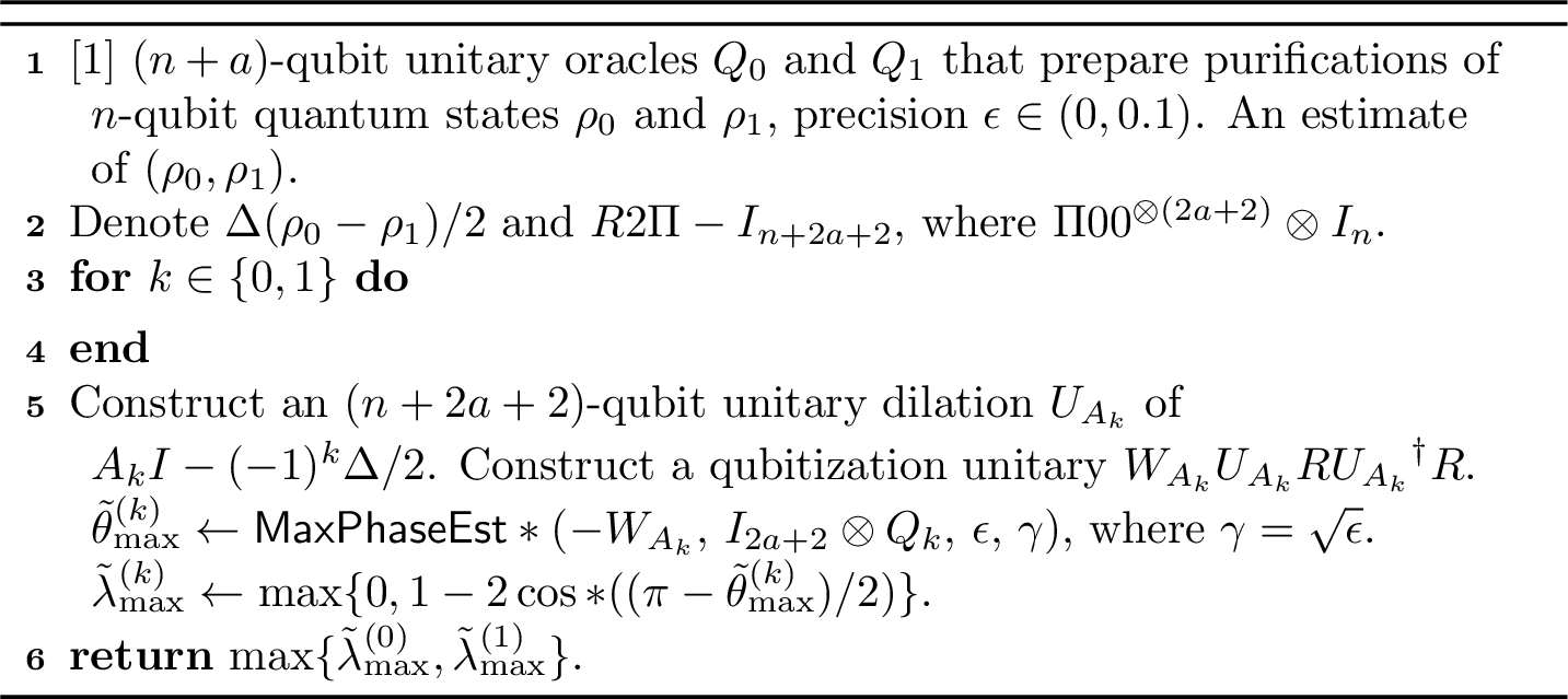
First we analyze the complexity of 2. Note that the unitary dilation \(U_{A_k}\) can be implemented using \(O(1)\) queries to \(Q_0\) and \(Q_1\) by 2 and linear combination of unitaries [42]. The qubitization unitary \(-W_{A_k}\) uses \(O(1)\) queries to \(U_{A_k}\). Taking \(\gamma = \sqrt{\epsilon}\), the subroutine \(\mathsf{MaxPhaseEst}(-W_{A_k}, I_{2a+2}\otimes Q_k, \epsilon, \gamma)\) uses a total number of \(O(\log(1/\epsilon)/\epsilon^{3/2})\) queries to \(Q_0\) and \(Q_1\). Therefore, the total number of queries to \(Q_0\) and \(Q_1\) is \(O(\log(1/\epsilon)/\epsilon^{3/2})\).

Next, we prove the correctness of the algorithm. We now consider the properties of \(\tilde{\theta}^{(k)}_{\max}\) for each \(k \in \{0, 1\}\). For convenience, here we assume that \(\lambda_{\max}\rbra{(-1)^k\Delta} \geq \epsilon\) (and the corner case where \(\lambda_{\max}\rbra{(-1)^k\Delta} < \epsilon\) will be discussed later). Note that the random variable \(\tilde{\theta}^{(k)}_{\max}\) is the output of \(\mathsf{MaxPhaseEst}\ab*(-W_{A_k},\, I_{2a+2} \otimes Q_k,\, \epsilon,\, \gamma)\), where \(\gamma = \sqrt{\epsilon}\). Then, it holds (shown later) that \[\label{eq:subroutine95ouput95mixed} \Pr\sbra[\Big]{\abs[\big]{\tilde{\theta}^{(k)}_{\max} - \theta_{\max}^{(k)} }\leq \epsilon} \geq 0.99, \qquad \text{where } \theta_{\max}^{(k)} = \pi + 2\arccos\ab\Big(\frac{1-\lambda_{\max}((-1)^k\Delta)}{2}).\tag{22}\] Therefore, when we take \[\tilde{\lambda}_{\max}^{(k)} = \max\ab\bigg\{0, 1 - 2\cos\ab\Big(\frac{\pi - \tilde{\theta}_{\max}^{(k)}}{2})\},\] and return \(\tilde{\lambda}_{\max} = \max\{\tilde{\lambda}_{\max}^{(0)}, \tilde{\lambda}_{\max}^{(1)}\}\), it holds that \[\label{eq:error95two95mixed} \Pr\sbra*{\abs[\big]{\tilde{\lambda}_{\max} - \Tinfty(\rho_0, \rho_1)} \leq \epsilon} \geq 0.99^2 > 0.98.\tag{23}\] To see this, note that \(\Tinfty(\rho_0, \rho_1) = \max\{\lambda_{\max}(\Delta), \lambda_{\max}(-\Delta)\}\) by definition. Therefore, by the mean value theorem, there exists some \(\xi^{(k)}\) between \(\theta_{\max}^{(k)}\) and \(\tilde{\theta}_{\max}^{(k)}\) such that \[\begin{align} \abs{\tilde{\lambda}_{\max}^{(k)} - \lambda_{\max}((-1)^k\Delta)} &= \abs[\Big]{\sin\ab\Big(\frac{\xi^{(k)}-\pi}{2})} \abs{\tilde{\theta}_{\max}^{(k)} - \theta_{\max}^{(k)}}. \end{align}\] Since \(\abs{\sin\ab((\xi-\pi)/2)} \leq 1\), we have \[\Pr\sbra*{\abs[\big]{\tilde{\lambda}_{\max}^{(k)} - \lambda_{\max}((-1)^k\Delta) }\leq \epsilon} \geq 0.99,\] which gives 23 . Therefore, 2 returns an estimate of \(\Tinfty(\rho_0, \rho_1)\) to within additive error \(\epsilon\).

To complete the proof, it remains to prove that the output of two subroutines satisfy the condition in 22 . We begin with the analysis on the subroutine \(\mathsf{MaxPhaseEst}(-W_{A_0}, I_{2a+2} \otimes Q_0, \epsilon, \gamma)\). To show that applying the quantum maximum phase estimation algorithm in 6 gives a result satisfying 22 , we prove the following properties in order.

1. The eigenphases of \(-W_{A_0}\) are in \([0, 2\pi - 2\epsilon)\), and the largest eigenphase of \(-W_{A_0}\) is \(\theta_{\max}^{(0)} = \pi + 2\arccos\ab((1-\lambda_{\max}(\Delta))/{2})\).

2. The state preparation unitary \(I_{2a+2} \otimes Q_0\) prepares a state that has an overlap at least \(\gamma = \sqrt{\epsilon}\) with the top eigenspace of \(-W_{A_0}\).

Let \(d=2^n\) be the dimension of the quantum states \(\rho_0\) and \(\rho_1\). For \(j\in \{1,\dots, d\}\), let \(\ket{v_j}\) denote an eigenvector of \(\Delta\) with eigenvalue \(\lambda_j\), i.e., \(\Delta\ket{v_j} = \lambda_j \ket{v_j}\), then \(\ket{v_j}\) is also an eigenvector of \(A_0\) such that \[A_0 \ket{v_j} = \mu_j \ket{v_j}, \qquad \mu_j \coloneq \frac{1-\lambda_j}{2}.\] Note that the eigenvalues of \(\Delta\) are in \([-1/2, 1/2]\), and therefore the eigenvalues of \(A_0\) are in \([1/4, 3/4]\).

Let \(\ket{u_j} = \ket{0}^{\otimes \rbra{2a+2}}\otimes\ket{v_j}\), and define \[\ket{u_j^\perp} \coloneq \frac{U_{A_0}\ket{u_j} - \mu_j\ket{u_j}}{\sqrt{1 - \mu_j^2}}.\] By 5, since \(\abs{\mu_j}<1\), the qubitization unitary \(W_{A_0}\) has eigenvectors \[\begin{align} \ket{\phi^{\pm}_{j}} & = \frac{1}{\sqrt{2}} \rbra[\big]{ \ket{u_j} \mp i \ket{u_j^\perp}}, \end{align}\] with \(W_{A_0} \ket{\phi^{\pm}_{j}} = e^{\pm i \vartheta_j} \ket{\phi^{\pm}_{j}}\), where \[\vartheta_j \coloneq 2\arccos(\mu_j) = 2\arccos\ab\Big(\frac{1-\lambda_j}{2}).\] Moreover, let \(\mathcal{P} \mathrel{\vcenter{:}}= \spanspace\set{\ket{u_j}}{1 \leq j \leq 2^n}\), \(\mathcal{Q} \coloneq \spanspace\set{\ket{u_j^\perp}}{1 \leq j \leq 2^n}\), and \(\mathcal{M} = \rbra{\mathcal{P} + \mathcal{Q}}^{\perp}\), then every nonzero vector \(\ket{\phi'} \in \mathcal{M}\) is an eigenvector of \(W_{A_0}\) with eigenphase \(0\), i.e., \(W_{A_0} \ket{\phi'} = \ket{\phi'}\).

Since the function \(\arccos((1-x)/{2})\) is strictly monotonically increasing on \([-1/2, 1/2]\), for increasing eigenvalues of \(\Delta\), \[\lambda_1 \leq \lambda_2 \leq \cdots \leq \lambda_{d},\] we have \[\vartheta_1 \leq \vartheta_2 \leq \cdots \leq \vartheta_{d}, \quad\text{where } \vartheta_{j} \in \ab[2\arccos\ab(3/4), 2\arccos\ab(1/4)] \subset (0, \pi-2\epsilon).\] Now we add a global phase \(e^{i\pi}\) to \(W_{A_0}\), i.e., \(e^{i\pi}W_{A_0} = - W_{A_0}\). The phases of \(- W_{A_0}\), denoted by \(\theta^{\pm}_{j} = \pi \pm \vartheta_j\), lie in \([0, 2\pi-2\epsilon)\) as \(\pi - \vartheta_j \in (0,\pi-2\epsilon)\) and \(\pi + \vartheta_j \in (\pi,2\pi-2\epsilon)\). The largest phase of \(- W_{A_0}\), denoted by \(\theta_{\max}^{(0)} \coloneq \max_j\{\theta^{\pm}_{j}\} = \max_j\{\theta^{+}_{j}\}\), clearly corresponds to the largest eigenvalue of \(\Delta\), \[\label{eq:max95eigenphase} \theta_{\max}^{(0)} = \pi+\vartheta_{N} = \pi + 2\arccos\ab(\frac{1-\lambda_{\max}(\Delta)}{2}).\tag{24}\]

Then we show that the state preparation unitary \(I_{2a+2} \otimes Q_0\) prepares a state that has an overlap at least \(\gamma = 1/2\) with the top eigenspace of \(-W_{A_0}\). The unitary \(I_{2a+2} \otimes Q_0\) prepares the input state \[\ket{\Psi_0} \coloneq (I_{2a+2} \otimes Q_0) \ket{0}^{\otimes \rbra{n+3a+2}} = \ket{0}^{\otimes \rbra{2a+2}} \ket{\psi_0}\] where \(\ket{\psi_0}\) is the purification of the state \(\rho_0\). By 8, the overlap between the input state and the top eigenspace of \(-W_{A_0}\) is at least \[\begin{align} \sum_{j:\theta^{+}_{j} = \theta_{\max}^{(0)}} \norm[\big]{(\bra{\phi_{j}^{+}}\otimes I_a) \ket{\Psi_0}}_2^2 &= \sum_{j:\theta^{+}_{j} = \theta_{\max}^{(0)}} \norm[\Big]{\ab\Big(\frac{1}{\sqrt{2}} \ab\big( \bra{u_j} + i \bra{u_j^\perp})\otimes I_a) \ket{\Psi_0}}_2^2 \\ &\geq \sum_{j:\theta^{+}_{j} = \theta_{\max}^{(0)}} \norm[\Big]{\frac{1}{\sqrt{2}}\ab\big(\bra{u_j} \otimes I_a) \ket{\Psi_0}}_2^2\\ &= \sum_{j:\lambda_{j}=\lambda_{\max}(\Delta)} \norm[\Big]{\frac{1}{\sqrt{2}}\big( \bra{0}^{\otimes {2a+2}} \otimes \bra{v_j} \otimes I_a)\ab\big(\ket{0}^{\otimes \rbra{2a+2}} \otimes \ket{\psi_0})}_2^2\\ &= \sum_{j:\lambda_{j}=\lambda_{\max}(\Delta)} \norm[\Big]{\frac{1}{\sqrt{2}}\big( \bra{v_j} \otimes I_a)\ket{\psi_0}}_2^2\\ &= \frac{1}{2} \norm[\big]{\ab\big( \Pi_{\max}^{(\Delta)}\otimes I_{a})\ket{\psi_0}}_2^2\\ &\ge \lambda_{\max}(\Delta). \end{align}\] With \(\lambda_{\max}(\Delta) \geq \epsilon\), we can take \(\gamma = \sqrt{\epsilon}\). Therefore, by 6, the maximum phase estimation algorithm \(\mathsf{MaxPhaseEst}(-W_{A_0}, I_{2a+2} \otimes Q_0, \epsilon, \gamma)\) uses \(O(1/\sqrt{\epsilon})\) queries to \(Q_0\) and \(O(\log(1/\epsilon)/\epsilon^{3/2})\) queries to \(-W_{A_0}\), outputs an estimate \(\tilde{\theta}_{\max}^{(0)}\) such that \[\Pr\sbra[\Big]{\abs[\big]{\tilde{\theta}^{(0)}_{\max} - \theta_{\max}^{(0)} }\leq \epsilon} \geq 0.99,\] as in 22 for \(k=0\).

Note that if \(\lambda_{\max}(\Delta) \in [0, \epsilon)\), taking \(\gamma = \sqrt{\epsilon}\) may not satisfy the overlap promise since \(\gamma^2 = \epsilon > \lambda_{\max}(\Delta)\). However, even without the overlap promise, the maximum phase estimation algorithm \(\mathsf{MaxPhaseEst}(-W_{A_0}, I_{2a+2} \otimes Q_0, \epsilon, \gamma)\) still outputs an estimate \(\tilde{\theta}_{\max}^{(0)}\), and with probability at least \(0.99\), there exists an eigenphase \(\theta_j^{\pm}\) of \(-W_{A_0}\) such that \(\abs{\tilde{\theta}_{\max}^{(0)} - \theta_j^{\pm}} \leq \epsilon\). Let \(f(\theta) = 1 - 2\cos((\pi - \theta)/2)\), by the mean value theorem, there exists a point \(\xi^{(0)}\) between \(\tilde{\theta}_{\max}^{(0)}\) and \(\theta_j^{\pm}\) such that \[\begin{align} \abs{f(\tilde{\theta}_{\max}^{(0)}) - f(\theta_j^{\pm})} &= \abs{f'(\xi^{(0)})} \abs{\tilde{\theta}_{\max}^{(0)} - \theta_j^{\pm}}\\ &= \abs[\Big]{\sin\ab\Big(\frac{\xi^{(0)}-\pi}{2})} \abs{\tilde{\theta}_{\max}^{(0)} - \theta_j^{\pm}}\\ &\leq \abs{\tilde{\theta}_{\max}^{(0)} - \theta_j^{\pm}}\\ &\leq \epsilon. \end{align}\] By definition, \(f(\theta_j^{\pm}) = \lambda_{j}\), thus we have \[f(\tilde{\theta}_{\max}^{(0)}) \leq \lambda_j + \epsilon \leq \lambda_{\max}(\Delta) + \epsilon.\] Since \(0 \leq \lambda_{\max}(\Delta) < \epsilon\), taking \(\tilde{\lambda}_{\max}^{(0)} = \max\{0, f(\tilde{\theta}_{\max}^{(0)})\}\) still guarantees that \[\Pr\sbra[\Big]{\abs[\big]{\tilde{\lambda}^{(0)}_{\max} - \lambda_{\max}(\Delta) }\leq \epsilon} \geq 0.99.\]

Similarly, we can analyze the subroutine \(\mathsf{MaxPhaseEst}(-W_{A_1}, I_{2a+2}\otimes Q_1, \epsilon, \gamma)\) by replacing \(\Delta\) with \(-\Delta\). Note that we have \(\norm{\ab*(\Pi_{\max}^{(-\Delta)}\otimes I_{a})\ket{\psi_1}}_2^2 \ge 2\lambda_{\max}(-\Delta)\) by symmetry. We can use the same analysis above to show that the algorithm \(\mathsf{MaxPhaseEst}(-W_{A_1}, I_{2a+2} \otimes Q_1, \epsilon, \gamma)\) uses \(O(1/\sqrt{\epsilon})\) queries to \(Q_1\) and \(O(\log(1/\epsilon)/\epsilon^{3/2})\) queries to \(-W_{A_1}\), outputs an estimate \(\tilde{\theta}_{\max}^{(1)}\) such that \[\Pr\sbra[\Big]{\abs[\big]{\tilde{\theta}^{(1)}_{\max} - \theta_{\max}^{(1)} }\leq \epsilon} \geq 0.99,\] as in 22 for \(k=1\). ◻

Proof. This is obtained immediately by 3 using the query complexity \(O\rbra{\log(1/\epsilon)/\epsilon^{3/2}}\) given in 5, which gives the sample complexity \(O\rbra{\log^2(1/\epsilon)/\epsilon^{3}}\). ◻