SAVER: Stochastic Adaptive Variance-Driven Exploration and Reconstruction for Low-Dose Computed Tomography
July 04, 2026
Introduction↩︎
Computed tomography (CT), first introduced by Hounsfield in the early 1970s, revolutionized diagnostic radiology by enabling non-invasive visualization of internal anatomy [1]. Over the past decades, continuous technological advances from early single-slice scanners to modern multi-slice and dual-energy CT systems have significantly improved spatial resolution, acquisition speed, and clinical applicability [2]. As a result, CT has become one of the most widely used imaging modalities for diagnosing a broad range of diseases. However, the growing use of CT has also raised concerns about the cumulative risk associated with ionizing radiation exposure. Consequently, reducing radiation dose while maintaining diagnostic image quality has become a central objective in CT research, following the principle of “as low as reasonably achievable” (ALARA) [3].
To address this issue, extensive research has focused on both hardware and computational approaches. Hardware-based strategies include beam filtration and detector improvements, while software-based approaches primarily rely on advanced image reconstruction techniques. In particular, iterative reconstruction (IR) [4], [5] and compressed sensing (CS) [6], [7] methods have demonstrated strong capabilities in reconstructing high-quality images from sparse-view or limited-angle measurements. These approaches have significantly improved the feasibility of low-dose CT [8], [9], when the underlying assumption holds such as sparsity in the domain to be monitored for a given sample. However, including IR and CS approaches, most existing CT acquisition strategies pre-design how to irradiate X ray to a sample in question irrespective of underlying structural complexity of the sample, and do not explicitly optimize the irradiation pattern, e.g., number of rays per angle, on the fly during the measurements with fewer a priori assumption on the sample.
Uniform angular sampling of X-ray irradiation means that the buried 2D (3D) structure of a sample is constructed from a set of X-ray absorption distributions resulting from uniform irradiation equally for different angles. This corresponds to implicitly assuming that structural information (complexity) is evenly distributed across projection angles (e.g., circle or sphere). In practice, however, anatomical structures often exhibit significant anisotropy and spatial heterogeneity (See Fig. 1). As a result, certain projection angles contain significantly more structural information than others, while many measurements contribute only marginally to reconstruction quality. From an information-efficiency perspective, this suggests that conventional fixed-geometry scanning may allocate radiation dose inefficiently by acquiring redundant projections that provide limited new information [10], [11].
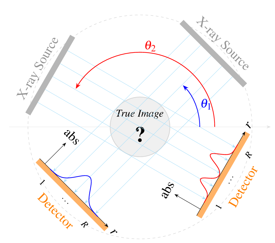
Motivated by this, we propose an adaptive CT acquisition framework that treats projection selection as a sequential decision problem, where the system selects and acquires a single projection ray at each round. The proposed method prioritizes projection angles based on the sample variance of the observed projection data value, which serves as a proxy for structural complexity along each direction in Radon space. To balance global exploration of possible directions with focused sampling of informative ones, we introduce a stochastic scheduling strategy based on a Softmax policy with simulated annealing [12]–[14]. By dynamically allocating measurements toward projections with higher structural information, the proposed framework aims to improve reconstruction efficiency and maximize image quality per unit radiation dose.
Results and Discussion↩︎
Problem Setup↩︎
In this study, the image reconstruction problem in CT is formulated as a linear inverse problem in which an unknown image vector is estimated from sequential projection measurements. The discrete representation of the imaging geometry and the construction of the corresponding linear system are illustrated in Figure 2.
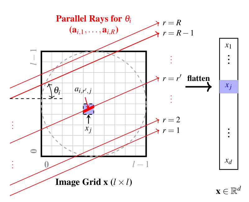
Let the unknown image be represented by a vector \(\mathbf{x} \in \mathbb{R}^{d}\), where \(d\) denotes the total number of pixels in the image. Specifically, the continuous attenuation coefficient distribution is discretized into a finite grid of pixels, and each element of \(\mathbf{x}\) represents the attenuation coefficient associated with a single pixel. The set of available projection angles is defined as \(\Theta=\{\theta_i=i\Delta\theta|i=0,1,\ldots,K-1\}\), where \(\Delta\theta\) denotes the angular step size in degrees and \(K = \left\lfloor \frac{180}{\Delta\theta} \right\rfloor\) is the total number of discrete angles in the range \([0,180)\). Given \([K] \mathrel{\vcenter{:}}= \{0, 1, \dots, K-1\}\), for each angle index \(i \in [K]\), let \(R\) denote the number of available irradiation positions. For the \(r\)-th irradiation position (\(r \in \{1, 2, \dots, R\}\)), we define a vector \(\mathbf{a}_{i,r}\). The \(j\)-th element of \(\mathbf{a}_{i,r}\) represents the intersection length between the \(r\)-th ray at angle \(i\) and the \(j\)-th pixel (\(j \in \{1, 2, \dots, d\}\)). These vectors are computed using Joseph’s reprojection method [15].
In the proposed framework, a projection measurement (referred to as a projection data value) is acquired sequentially, which represents the line integral of the single projection ray attenuation coefficients along a specific ray path through the object in each acquisition round. (For proof-of-concept simulation experiment, we imposed a single projection ray rather than predetermined, uniformly distributed multiple rays irrespective of angles per round). At each round \(t = 1, 2, 3, \ldots\), the algorithm selects an angle index \(i_t\). Then, an irradiation position \(r_t\) is randomly selected from the unused position candidates up to round \(t\). The observed projection data value \(y_t\) is defined as: \[\label{eq:projection} y_t = \mathbf{a}_{i_t,r_t}^{\top} \mathbf{x} + \epsilon_t,\tag{1}\] where for the purposes of our simulations, we assume \(\epsilon_t \sim \mathcal{N}(0,\sigma_B^2)\) to be independent Gaussian measurement noise with variance \(\sigma_B^2\). After rounds of \(t\), the observation vector becomes \(\mathbf{y}_t=(y_1,y_2,\ldots,y_t)^\top\in\mathbb{R}^t\). Let \(A_t \mathrel{\vcenter{:}}= \left(\mathbf{a}_{i_1,r_1}, \mathbf{a}_{i_2,r_2},\ldots,\mathbf{a}_{i_t,r_t}\right)^\top\in\mathbb{R}^{t\times d}\) denote the corresponding measurement matrix. Here, \(\mathbf{y}_t\) that would be acquired at the time when all irradiationable points are exhausted over all angles including less important angles corresponds to the set of absorption profiles at all projection angle in the parallel irradiation beam scheme shown in Figure 1. The image estimate \(\hat{\mathbf{x}}_t\) is obtained as the solution of the following minimization problem based on Tikhonov regularization [16]: \(\hat{\mathbf{x}}_t \mathrel{\vcenter{:}}= \operatorname{argmin}_{\mathbf{x}\in\mathbb{R}^d}\;\left(\|A_t\mathbf{x} - \mathbf{y}_t\|_2^2 + \frac{\sigma_B^2}{\xi^2}\|\textcolor{black}{\mathbf{x}}\|_2^2\right)\). The parameter \(\xi^2\) controls the variance of the Gaussian prior distribution imposed on the unknown image \({\mathbf{x}}\) and serves as a hyperparameter. The stable estimate can be computed via solving the normal equation as \[\label{eq:normal32eq} \hat{\mathbf{x}}_t=\left(A_t^\top A_t + \frac{\sigma_B^2}{\xi^2} I \right)^{-1}A_t^\top \mathbf{y}_t,\tag{2}\] where \(I\) denotes the identity matrix. In this study, we aim to develop an adaptive control algorithm that computes an estimate \(\hat{\mathbf{x}}\) close to the true image \(\mathbf{x}\) while using as fewer X-ray projections as possible.
Proposed Framework: SAVER↩︎
To address sampling inefficiency, we introduce Stochastic Adaptive Variance-Driven Exploration and Reconstruction (SAVER). The core idea is to treat the CT acquisition as a sequential decision process where the system dynamically reallocates radiation dose based on structural complexity of the sample object. The working hypothesis is that the higher the variance in projection data values (associated with the corresponding X-ray absorption distribution) along a specific projection angle, the more the structural information of the sample object is concentrated in reconstructing the image \(\mathbf{x}\). SAVER prioritizes increasing the number of rays for such informative directions to maximize reconstruction fidelity per dose, ensuring that each specific projection ray is sampled without repetition.
Let \(Y_i(t)\) be the set of projection data values obtained from angle index \(i\) up to round \(t\), with the total number of the observations \(n_i(t) = |Y_i(t)|\). The sample variance for index \(i\) is computed as \[\label{eq:samplevariance} \hat{\sigma}_i^2(t) \mathrel{\vcenter{:}}= \frac{1}{n_i(t)} \sum_{y \in Y_i(t)} y^2 -\left( \frac{1}{n_i(t)} \sum_{y \in Y_i(t)} y \right)^2.\tag{3}\] The sample variance \(\hat{\sigma}_i^2(t)\) quantifies structural variability observed from index \(i\) and is updated under the process of measurements. Especially when the values of \(n_i(t)\) are small, \(\hat{\sigma}_i^2(t)\) can vary abruptly across angles, and thus we employ robust scaling based on the median and the interquartile range (IQR), insensitive to outliers, defined by \(\tilde{\sigma}_i(t) =\frac{ \hat{\sigma}_i^2(t) - \mathrm{median}(\mathbf{v}(t))}{ \mathrm{IQR}(\mathbf{v}(t)) }\), where \(\mathbf{v}(t)\) is a set of \(\hat{\sigma}_i^2(t)\) whose total number of points that have been irradiated up to round \(t\) is smaller than the maximum and \(\mathrm{IQR}(\mathbf{v}(t))\) denotes the interquartile range of \(\mathbf{v}(t)\). The normalized value \(\tilde{\sigma}_i(t)\) is then used as the score for the Softmax-based angle selection policy. The next projection angle is selected probabilistically via a “temperature”-controlled Softmax function: the selection probability of projection angle \(i\) at round \(t\) over an angle set (denoted by \(F(t)\)) whose total number of points that have been irradiated up to round \(t\) is smaller than the allowance is defined by \[P_i(t) \mathrel{\vcenter{:}}= \frac{ \exp\!\left(\frac{\tilde{\sigma}_i(t)}{T_t} \right) }{ \sum_{j\in F(t)} \exp\!\left( \frac{\tilde{\sigma}_j(t)}{T_t} \right) }. \label{eq:softmax}\tag{4}\] \(T_t (> 0)\) denotes the “temperature” parameter to control sampling over different angles, i.e., when \(T_t\) is larger (smaller), the probability distribution becomes more (less) uniform, promoting exploratory sampling across projection angles (exploitation of informative orientations). In this paper, to gradually shift the sampling behavior from exploration to exploitation, \(T_t\) is updated by \(T_t=\max \left( T_{\min}, \frac{T_{\text{initial}}}{1 + \eta (t-2K)} \right)\), where \(T_{\text{initial}}\) (\(T_{\min}\)) denotes the initial temperature (the minimum temperature), and \(\eta\) represents the annealing rate. This annealing strategy ensures that the algorithm initially explores a wide range of projection angles and progressively concentrates measurements on orientations that exhibit higher structural variability.
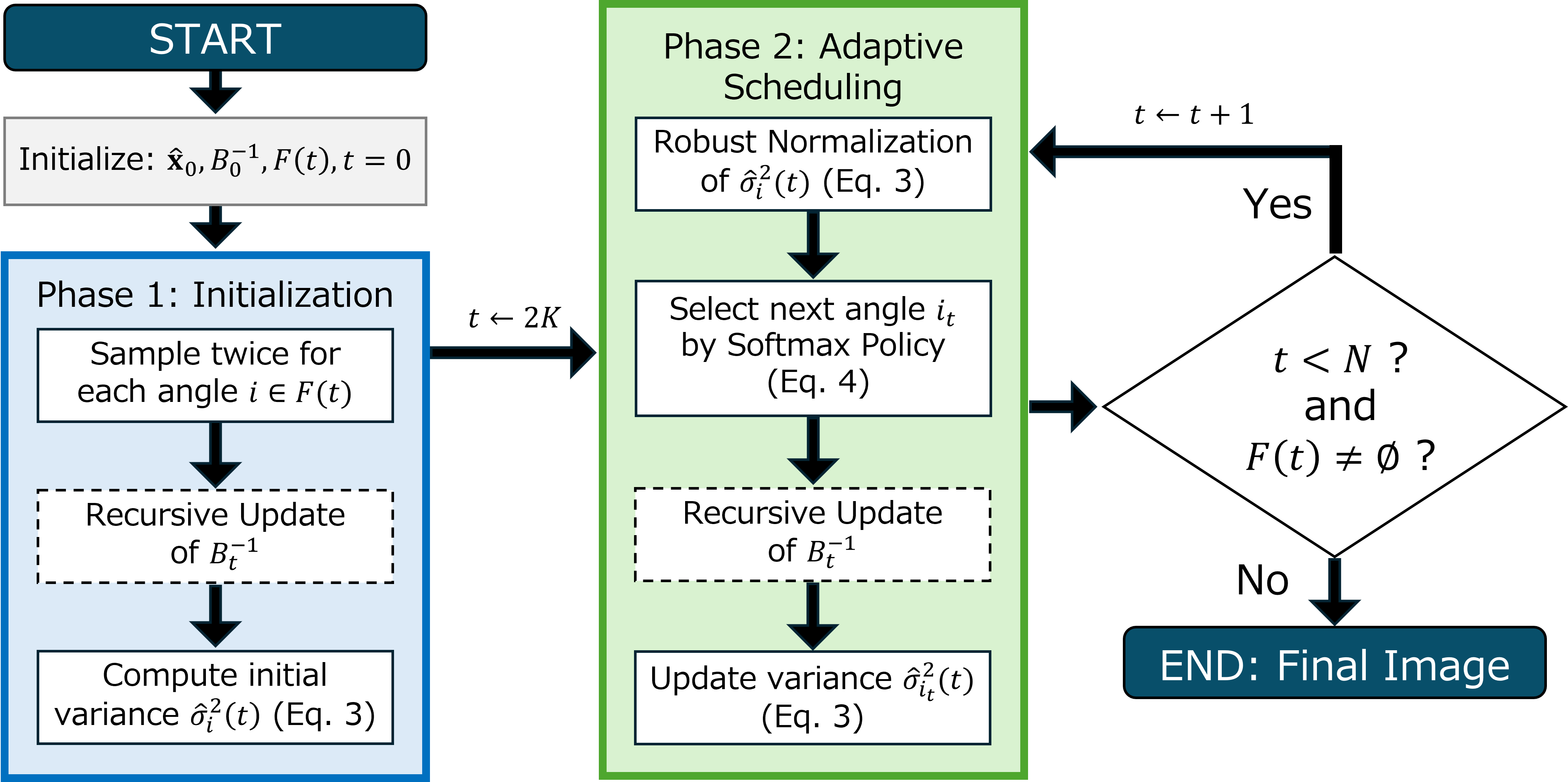
Unlike conventional fixed geometries, SAVER utilizes a probabilistic scheduling policy that balances the exploration of unknown projection angles with the exploitation of highly informative directions identified through real-time variance analysis. The overall operational workflow of the proposed method composed of the two-stage process (initialization and adaptive scheduling) is illustrated in Figure 8 and the role of each hyperparameter is summarized in Table 1 in the Methods section. It should be noted that SAVER does not necessarily require the inverse matrix calculation \(B_t^{-1}\) and restore the updated image \(\hat{\mathbf{x}}_t\) at every round for adaptive decision-making. The image reconstruction process can be performed only when necessary, thereby significantly reducing the total computational overhead during the acquisition phase (In this paper, however, we reconstructed and updated the underlying image \(\hat{\mathbf{x}}_t\) using Woodbury Matrix Identity presented in the Methods section, for the purpose of elucidation of the reconstruction performance of SAVER and its variants, especially to compare with the conventional scheme (Random) without referring any variance information).
Experimental Setup↩︎
We conduct numerical simulations under a simplified CT imaging model assuming a monochromatic X-ray beam and a linear attenuation process. Under this model, each projection measurement corresponds to the line integral of the object’s attenuation coefficient, while physical effects such as beam hardening, scattering, and refraction are neglected. To evaluate the proposed method, we perform experiments on 8 computational phantoms (\(32\times32\) pixels; Figure 3) representing diverse structural characteristics. For all projection angles, the number of available irradiation positions was set to \(R=32\), matching the image size.
The performance of the proposed framework was evaluated against several adaptive and non-adaptive baselines. In addition to the original SAVER algorithm, we also consider three practical methods and four oracle-guided reference methods.
Random: Selects a projection angle \(i_t\) and an irradiation position \(r_t\) uniformly at random from the set of all available irradiation positions without replacement (=no irradiation is applied for the same position).
AIRS (Axis-Initialized Random Sampling): Before random sampling begins, AIRS first utilizes (exhausts) all irradiation positions at \(0^\circ\) and \(90^\circ\), which correspond to the principal horizontal and vertical directions of the space-fixed image grid (how an object to be measured is lying in the grid is, of course, assumed to be unknown). After this deterministic initialization, the remaining irradiation positions are selected uniformly at random without replacement.
SAVER-A: SAVER-A first exhausts the irradiation positions at \(0^\circ\) and \(90^\circ\). After this axis-prior initialization, the algorithm follows SAVER.
MAX-V (Oracle): Selects a projection angle \(i_t\) from the angle whose true variance is the largest, sequentially in descent order up to the smallest true variance angle, each of which all irradiation positions are sampled for the chosen angle via Round-Robin (Remind that unless irradiating the object in full from all angles, one cannot acquire true variances of the projection data values for all angles).
MIN-V (Oracle): Selects a projection angle \(i_t\) from the angle whose true variance is the smallest, sequentially in ascent order up to the largest true variance angle, each of which all irradiation positions are sampled for the chosen angle via Round-Robin.
SAVER-O (Oracle): Selects a projection angle \(i_t\) according to Softmax probabilities using true variances of all angles. Projection angles whose irradiation positions have been fully consumed are excluded from the probability calculation. No explicit initialization phase is required.
SAVER-AO (Axis-Oracle): First exhausts the irradiation positions at \(0^\circ\) and \(90^\circ\) in the same manner as SAVER-A, and subsequently follows the same oracle-guided Softmax scheduling as SAVER-O.
The performance gap between MAX-V and MIN-V serves as a direct measure of the utility of the variance metric in prioritizing structural information.
![Figure 3: 8 synthetic phantoms used in the experiments: (1) Rectangle, (2) Hollow Square, (3) Triangle, (4) Cross, (5) Checkerboard, (6) Stripes, (7) Gradient, (8) Shepp-Logan [17]. All images have a resolution of 32\times32 pixels.](/article/2607.03761/figures/8version/phantoms8.png "fig:")
In our simulations, the total number of acquisition rounds \(N\) was set to \(N=500\). Each acquisition round here corresponds to an X-ray irradiation of a certain position for a chosen angle. Note that without noise, \(N\simeq 800\) is a sufficient number of irradiation points to reconstruct the underlying image accurately in the present setting. Each measurement is given by Eq. 1 . Stacking observations up to round \(N\), we obtain a linear system \(\mathbf{y}_N=A_N\mathbf{x}\), where \(A_N\in\mathbb{R}^{N\times d}\) consists of row vectors. In the noiseless case, accurate reconstruction requires that this system is (approximately) inverted, i.e., the number of linearly independent measurements is comparable to the number of effective unknowns. For an image of size \(l\times l\), the total number of pixels is \(d=l^2\). However, since reconstruction is restricted to the inscribed circular region, the effective number of unknowns is approximately \(d\times\frac{\pi}{4}=l^2\times\frac{\pi}{4}\). For \(l=32\), this yields \(32^2\times\frac{\pi}{4}=804.2477\ldots\). Therefore, \(N\simeq 800\) measurements are sufficient to reconstruct any object in the noiseless setting.
To investigate the robustness of the proposed framework against stochastic perturbations, two distinct measurement noise regimes were considered: a low-noise environment (\(\sigma_B = 10^{-6}\)), approximating a near-ideal scenario, and a high-noise environment (\(\sigma_B = 10^{-2}\)), which may reflect low S/N cases for actual CT observation. The configuration for the SAVER algorithm was standardized with an angular resolution of \(\Delta\theta = 3\) degree and a prior regularization parameter of \(\xi = 0.1\). To balance exploration and exploitation, we used a Softmax-based scheduling policy with temperature annealing (see Methods). The temperature parameter \(\textcolor{black}{T}_t\) controls the sharpness of the selection distribution and is gradually decreased to shift the policy from exploration to exploitation. In our experiments, \(\textcolor{black}{T}_t\) was initialized at \(\textcolor{black}{T}_{\text{initial}} = 1\) and decayed to \(\textcolor{black}{T}_{\min} = 0.1\) with annealing rates \(\eta \in \{1, 0.1, 0.01\}\). For each experimental configuration, the reconstruction process was repeated ten times using independent random seeds to ensure statistical significance. To ensure that the performance gains are invariant to the object’s orientation relative to the Cartesian image grid and to avoid potential grid bias, the phantom image in each of the ten independent trials was rotated by a random integer angle \(\alpha\in[0,45]^\circ\) prior to the acquisition process. This randomization ensures that the adaptive selection policy is evaluated on its ability to identify structural complexity regardless of how the object is aligned with the pixel grid. The reconstruction fidelity at each acquisition round \(t\) was quantified using the mean Structural Similarity Index Measure (SSIM) and its associated standard deviation, computed relative to the ground truth image within the inscribed circular field of view as defined in Eq. 5 . In the following sections, we primarily discuss the results obtained with the annealing rate \(\eta=0.01\) under a low-noise environment (\(\sigma_B = 10^{-6}\)). The results and discussion for other annealing rates (\(\eta=\textcolor{black}{0.1,1,10}\)) under both noise environments are provided in the Supplementary Information for comparative analysis.
Discussion↩︎
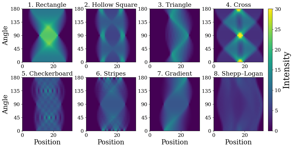
To begin, we show a sinogram representation of the 8 synthetic phantoms in Figure 4. They are graphical encodings of X-ray projections collected at multiple angles around objects. Each of them captures how X-ray intensity varies as the beam passes through the object from different directions. In this representation, the horizontal axis corresponds to detector position, while the vertical axis represents the projection angle. Sinogram contains not only the information needed to infer internal structures for each angle, and also importantly how inhomogeneous the information each angle carries is. One can see immediately that some phantoms such as 1. Rectangle, exhibit significantly different intensities (integrated over positions) depending on the angle, whereas other phantoms such as 8. Shepp-Logan, carry relatively uniform intensities across all angles, as expected from the phantom images.
Then, How much does the working hypothesis actually work in reconstructing the image \(\mathbf{x}\) based on the variances in projection data values (associated with the corresponding X-ray absorption distribution) along projection angles? Figure 5 presents the evolution of the SSIM as a function of the number of acquisition rounds under low-noise (\(\sigma_B = 10^{-6}\)) for the 8 phantoms.
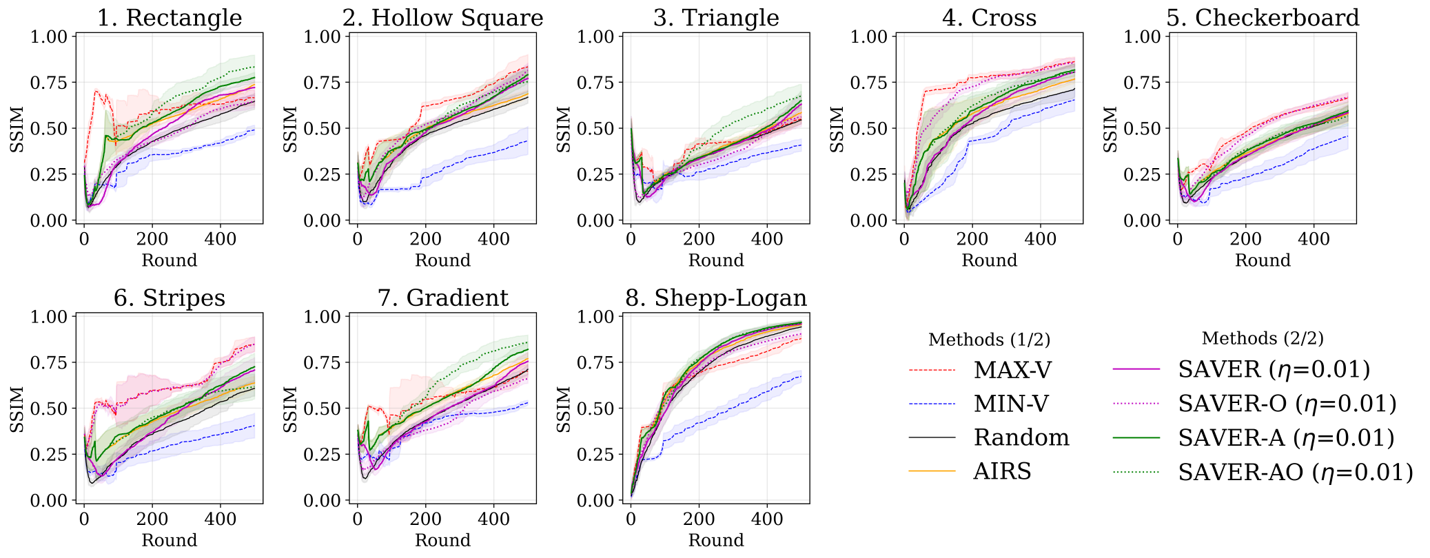
Let us first focus on the behaviors of the oracle methods, MAX-V (red dashed line) and MIN-V (blue dashed line) with the conventional scheme, Random (black solid line) without referring any variance information of the projection data values of angles. MIN-V generally exhibits the lowest SSIM performance across most rounds for all phantoms. This partially indicates that the lesser the variance of projection data values for angle, the lesser the importance of angles in capturing the object image. In turn, MAX-V tends to yield a high performance, especially for phantoms in which the projection angles have inhomogeneous importance in sinogram (Fig. 4) such as 1. Rectangle, 4. Cross, and 6. Stripes resulting in a substantial gap between MAX-V and MIN-V, and the baseline algorithm Random is located somewhere between the two. MAX-V performs better than Random notably during early rounds for those phantoms. MAX-V also exhibits a higher performance than Random in the reconstruction for phantoms 2. Hollow Square and 5. Checkerboard whose images (Fig. 3) are somehow symmetric as well as 7. Gradient.. In turn, for the phantoms whose variance information along projection angles are more homogeneous, such as 3. Triangle and 8. Shepp-Logan, MAX-V exhibits only comparative performance against Random. However, it may be noted that during early rounds (say, less than 50 rounds) MAX-V shows slightly higher performance than Random for these two phantoms. All these observation suggests that, especially for “structured” object where each projection angle carries uneven information for the underlying object, at least during early rounds, nonrandom choice of projection angles are effectively in capturing the underlying objects.
However, no one knows the underlying true variance of projection data values along angles a priori. This fundamental limitation necessitates an acquisition framework capable of estimating structural complexity in real-time, purely from the data acquired during the measurement process. The SAVER algorithm addresses this challenge through its two-stage operational workflow (as illustrated in Fig. 8): a deterministic initialization phase to establish baseline variance estimates, followed by an adaptive scheduling phase that probabilistically steers irradiation toward highly informative directions. By bridging the gap between unknown structural distributions and data-driven decision-making, SAVER transforms CT from a static process into a dynamic, sample-dependent exploration. The following subsections analyze how this mechanism effectively manages information scarcity and adapts to various sample geometries.
Information Scarcity and Algorithmic Efficiency↩︎
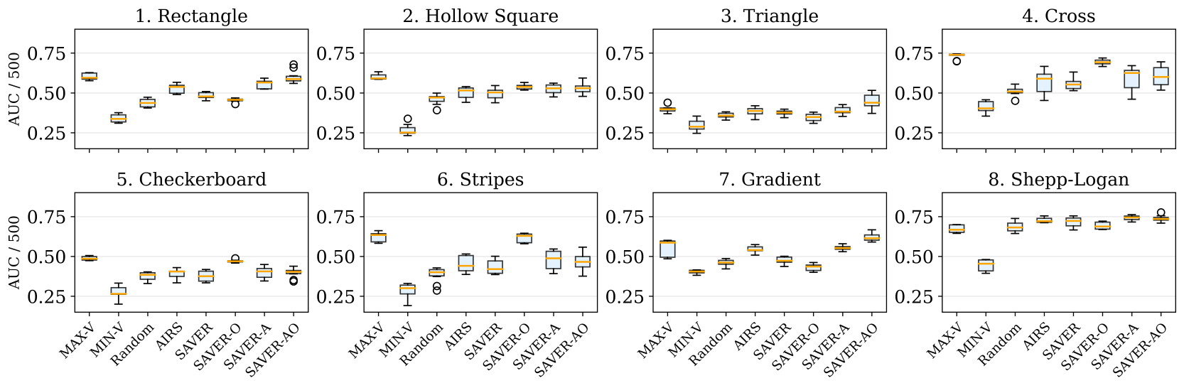
The efficacy of the SAVER framework is fundamentally rooted in its ability to exploit the structural anisotropy of the sample. As visually evident in the sinograms (Fig. 4), structural information is concentrated in narrow angular bands for objects with high geometric non-uniformity, such as 1. Rectangle, 4. Cross, and 6. Stripes. In Figure. 5, for 1. Rectangle, 4. Cross, and 6. Stripes phantoms, SAVER-A (green solid line) reaches the target fidelity significantly faster than conventional uniform sampling (Random) (black solid line), which does not account for structural heterogeneity. Note that SAVER-A also reach the target fidelity (slightly) faster than Random in 2. Hollow Square and 7. Gradient (8. Shepp-Logan). While the SSIM convergence curves as a function of acquisition rounds (Fig. 5) provide an overall comparison of algorithm performance across phantoms, their intrinsic complexity—arising from overlapping standard deviation bands and fluctuating recovery behavior over 8 distinct phantoms—limits detailed quantitative interpretation. To overcome these visual limitations, we introduce the normalized Area Under the Curve (AUC/500) for SSIM as a summary metric. Note that this AUC/500 is the integral of the SSIM curve and is distinct from the AUC of a Receiver Operating Characteristic (ROC) curve. By integrating the fidelity curve over the entire span of 500 acquisition rounds, the AUC provides a brief summary of the reconstruction performance, that is, not only for the final image quality but also for how close to a hypothetical case in which only the first one round can reconstruct the underlying object (SSIM \(\simeq 1\)) and consecutive rounds up to 500 maintain that quality. Figure 6 presents the box-whisker plots of AUC/500 for each algorithm with different phantoms. As seen in Figure 6, MIN-V has the lowest AUC/500 values for most phantoms, and MAX-V tends to yield higher in AUC/500 values than the others for the phantoms with heterogeneous importance in projection angles such as 1. Rectangle, 4. Cross, and 6. Stripes, including 2. Hollow Square and 5. Checkerboard. Note that AIRS improves the performance of Random especially for phantoms having heterogeneous preference in projection angles. In comparison between SAVER variants (SAVER and SAVER-A), SAVER-A exhibits better or at least equal performance to SAVER.
Analysis of Axis-Prior Initialization and Structural Heterogeneity↩︎
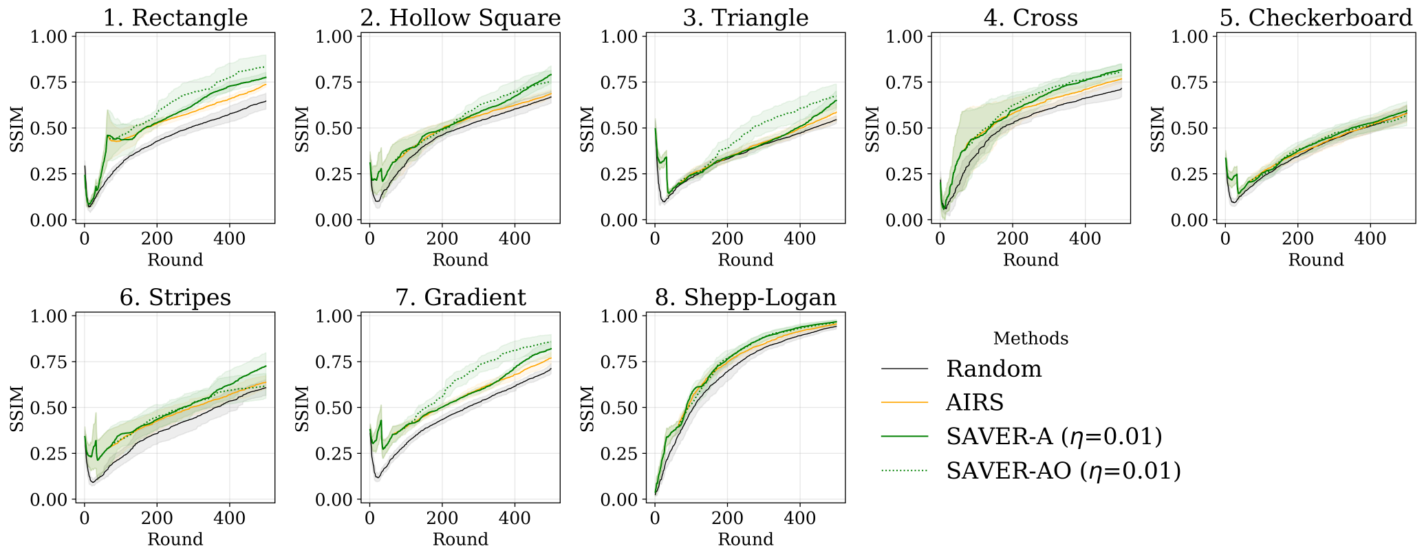
The core logic behind starting the acquisition with orthogonal projections (\(0^\circ\) and \(90^\circ\)) employed in AIRS, SAVER-A, and SAVER-A is rooted in early basis construction for the image estimate; a detailed mathematical interpretation regarding how this stabilizes the posterior covariance matrix and improves the conditioning of the sequential inverse problem is provided in the Supporting Information, Section 1. Figure 7 presents SSIM as a function of acquisition rounds only for the three Axis-Prior Initialization-based algorithms in addition to Random corresponding to the conventional algorithm in Figure 5. The performance gains observed in Figure 7 are directly dictated by the structural characteristics of the phantoms in Radon space. For phantoms exhibiting high structural anisotropy, such as 1. Rectangle, 4. Cross, and 6. stripes, the sinograms in Figure 4 reveal that information is concentrated within very narrow angular bands. In these cases, Figure 7 shows statistically significant performance gaps between SAVER-A (green solid line) and AIRS (orange solid line) in the exploitation stage where the annealing has been performed. While AIRS benefits from the initial stabilization of the axis-prior, its subsequent uniform random sampling fails to exploit the highly localized structural information. In contrast, SAVER-A utilizes real-time variance estimation to identify and concentrate radiation dose on the “informative” peaks seen in the sinogram, leading to a much steeper rise in SSIM during the early-to-mid acquisition rounds.
Conversely, for phantoms with more homogeneous or isotropic information distributions, such as 8. Shepp-Logan, the sinogram in Figure 4 shows relatively consistent intensity across the \(0^\circ-180^\circ\) range. Consequently, as seen in Figure 7, the performance gap between the four selected methods is narrower. In such cases, because most projection angles carry comparable amounts of information, the advantage of adaptive selection is reduced. However, it is noteworthy that SAVER-A still performs at or above the level of the AIRS and Random baselines, demonstrating that the stochastic scheduling policy does not “over-invest” in specific angles when the sample does not warrant it. In turn, for 5. Checkerboard having almost circular symmetric nature in shape more than 8. Shepp-Logan, most of all algorithms including SEVER-AO using the underlying true variance exhibit similar performance as non-adaptive baseline Random. The comparison in Figure 7 also highlights the behavior of phantoms such as 3. Triangle and 7. Gradient, indicating that, if the estimation of the underlying true variance would be tighter (more accurately estimated) (see SAVER-AO), SAVER-A should outperform the baseline AIRS as those exhibiting high structural anisotropy.
Overall, we observe that AIRS plateaus shortly after the initial axis-exhaustion phase. SAVER-A, however, successfully navigates the exploration-exploitation trade-off to find these critical off-axis directions. This confirms that while the axis-prior provides a necessary “warm-start” (as discussed in the Supplementary Information), it is the subsequent adaptive variance-driven scheduling that allows the system to transcend fixed geometric assumptions and adapt to the specific orientation and complexity of the individual sample.
Stability via Stochastic Selection Policy↩︎
The stability of the SAVER framework stems from its Softmax-based stochastic policy. Unlike deterministic greedy strategies that may over-invest in narrow angular ranges, the simulated annealing approach maintains a necessary degree of exploration. This results in the smooth and monotonic improvement of the SSIM observed across all phantoms in Figure 5. While the primary analysis focuses on this low-noise environment to elucidate the core principles of SAVER, the framework’s robustness against significant measurement noise (\(\sigma_B = 10^{-2}\)) is also confirmed. Under such high-noise regimes, the stochastic policy acts as a vital regularizer, preventing the system from becoming ill-conditioned. The detailed comparative analysis with oracle-guided greedy methods under noise is provided in the Supplementary Information (Figs. S1–S3).
Outlook↩︎
In summary, the efficiency of the SAVER framework is driven by its ability to adapt to the nonuniformity of information in the sinogram (See Fig. 4). While random sampling implicitly treats all projection angles as equally informative, SAVER dynamically reallocates radiation dose to the most critical ones. Overall, this study not only demonstrates the efficiency of adaptive sampling but also reveals that a stochastic policy is essential for maintaining stability under measurement noise, marking a significant step toward personalized, data-driven CT acquisition. The following are some of the problems to be uncovered in the forthcoming subjects in autonomous, data-driven design of irradiation profile in CT reconstruction.
First, while the proposed SAVER framework adaptively selects projection angles, the irradiation position within each selected angle is currently sampled in a simple sequential manner. Investigating more principled irradiation position selection strategies is an important next step. In particular, quasi–Monte Carlo (QMC) sampling, such as Sobol or Halton sequences [18], may provide a more uniform coverage of the detector coordinate and potentially improve reconstruction stability. Other space-filling designs, including Latin hypercube sampling [19] and blue-noise sampling [20], may also be explored to ensure more uniform and less correlated ray distributions. A systematic comparison of these sampling strategies should clarify their impact on reconstruction quality and sampling efficiency.
Second, the proposed approach currently focuses on selecting projection angles based on variance-driven exploration, without explicitly optimizing the posterior covariance of the reconstruction. Future work may incorporate principles from optimal experimental design to guide the selection of irradiation positions. In particular, D-optimality, which minimizes the determinant of the posterior covariance matrix, and A-optimality, which minimizes its trace, may provide principled criteria for sequentially selecting irradiation positions that maximally reduce reconstruction uncertainty [21]. Integrating such criteria with the SAVER framework is expected to lead to more efficient information acquisition and improved reconstruction accuracy.
Third, the current Softmax-based policy provides a simple mechanism for balancing exploration and exploitation. However, more principled bandit-based policies (as frameworks for sequential decision-making under uncertainty) [22] may yield stronger theoretical guarantees. In particular, upper confidence bound (UCB) [23] strategies are among the subjects to be addressed for projection-angle selection. By deriving tighter confidence intervals for the variance using concentration inequalities such as the McDiarmid inequality [24] or related bounds, it may be possible to design a theoretically grounded UCB policy tailored to the CT acquisition process.
Fourth, irradiation position selection can be guided not only by reconstruction uncertainty (in the present study) but also by downstream objectives such as lesion detectability or segmentation performance, which integrate task-driven acquisition strategies on multiobjective fashion. Combining the proposed adaptive acquisition strategy with modern learned reconstruction methods, including plug-and-play priors or diffusion-based reconstruction models, may also further enhance reconstruction quality under extremely low-dose conditions. Finally, the realization of our proposed framework to three-dimensional cone-beam CT [25], where the acquisition geometry introduces additional degrees of freedom and challenges, is one of the possible steps toward realization into real applications.
Fifth, as seen in Fig. 4, structural anisotropy exists not only angle axis but also position axis. In this paper, we focused only on the preferential selection of angles in reconstructing the underlying image but there exists room to optimize and design which positions are selected during the CT reconstruction. This is one of the on-going projects to be addressed in a separate paper.
Methods↩︎
Summary of Designed Parameters↩︎
The key user-defined parameters and their roles are summarized in Table 1. These parameters control the balance between exploration of unknown projection angles and exploitation of information acquired up to each round.
| Parameter | Description | Role in SAVER |
|---|---|---|
| \(\Delta\theta\) | Angular step size (degrees) | Defines the total number of discrete angles \(K\). |
| \(\xi^2\) | Prior regularization parameter | Controls the variance of the Gaussian prior on the image \(\mathbf{x}\). |
| \(T_{\text{initial}}\) | Initial temperature | Sets the initial level of randomness in the Softmax policy to promote global exploration. |
| \(T_{\text{min}}\) | Minimum temperature | Defines the baseline temperature to maintain a degree of exploration even in the late stages. |
| \(\eta\) | Annealing rate | Determines the speed of transition from broad exploration to focused exploitation of high-variance directions. |
| \(N\) | Total acquisition rounds | Represents the total radiation dose budget (total number of X-ray projection rays). |
Efficient Image Reconstruction via Woodbury Matrix Identity↩︎
To achieve real-time adaptive acquisition, the image estimate \(\hat{\mathbf{x}}_t\) can be updated at each round \(t\) as a new projection data value \(y_t\) (Eq. 1 ) is acquired. Solving the minimization problem in Eq. 2 directly requires inverting a \(d \times d\) matrix at every round, which entails a prohibitive computational cost of \(O(d^3)\). In this study, we implement an efficient recursive update scheme based on the Woodbury matrix identity (also known as the matrix inversion lemma) [26] to estimate the reconstruction fidelity of SAVER and its variants along consecutive rounds. This approach allows to compute the updated inverse matrix \(B_t^{-1} = (A_t^\top A_t + \frac{\sigma_B^2}{\xi^2}I)^{-1}\) using the result from the previous round \(B_{t-1}^{-1}\), reducing the per-update complexity to \(O(d^2)\). At each round \(t\), given the selected index \(i_t\) and irradiation position \(r_t\), the estimate \(\hat{\mathbf{x}}_t\) and the inverse covariance matrix \(B_t^{-1}\) are updated as follows:
\[\begin{cases} D_t = 1 + \mathbf{a}_{i_t, r_t}^\top B_{t-1}^{-1} \mathbf{a}_{i_t, r_t} \\ \mathbf{k}_t = (B_{t-1}^{-1} \mathbf{a}_{i_t, r_t}) / D_t \\ \hat{\mathbf{x}}_t = \hat{\mathbf{x}}_{t-1} + \mathbf{k}_t (y_t - \mathbf{a}_{i_t, r_t}^\top \hat{\mathbf{x}}_{t-1}) \\ B_t^{-1} = B_{t-1}^{-1} - \mathbf{k}_t (\mathbf{a}_{i_t, r_t}^\top B_{t-1}^{-1}) \end{cases}\]
where \(D_t\) is a scalar denominator and \(\mathbf{k}_t \in \mathbb{R}^d\) is the gain vector. The recursion is initialized with \(\hat{\mathbf{x}}_0 = \mathbf{0}\) and \(B_0^{-1} = \frac{\xi^2}{\sigma_B^2} I\). This recursive formulation enables the SAVER framework to perform high-speed, sequential image updates, which is essential for real-time projection selection.
While the current recursive update using the Woodbury identity reduces the complexity to \(O(d^2)\) per measurement, this remains computationally demanding for clinical resolutions (e.g., \(512\times512\) pixels). In such high-dimensional spaces, the storage and update of the inverse covariance matrix \(B_t^{-1}\) require significant memory and FLOPs. Future implementations may leverage domain-decomposition methods, low-rank approximations of the covariance matrix, or fast iterative solvers to maintain the real-time adaptability of SAVER in large-scale settings. Nevertheless, as highlighted in the operational workflow in Figure 8, the full restoration of the image \(\hat{\mathbf{x}}_t\) at every round is not mandatory for adaptive decision-making. Since the selection policy in SAVER is driven by the statistical variance of the observed projection data values, the image reconstruction process can be deferred to the final stage or performed only when necessary, thereby significantly reducing the total computational overhead during the acquisition phase.
Evaluation Metric↩︎
To evaluate the reconstruction quality, we employed the Structural Similarity Index Measure (SSIM) [27], which measures perceptual similarity by comparing luminance, contrast, and structural information between two images \(\mathbf{x}\) and \(\mathbf{y}\) \(\in \mathbb{R}^{32} \times \mathbb{R}^{32}\). In practice, SSIM is computed as the mean SSIM (MSSIM) over local sliding windows. For each pixel location \((i,j)\), a local window \(w_{i,j}\) of size \(7 \times 7\) was defined, and the local SSIM was computed as \(\mathrm{SSIM}_{i,j}(\mathbf{x},\mathbf{y}) = \frac{(2\mu_{i,j}^\mathbf{x} \mu_{i,j}^\mathbf{y} + C_1)(2\sigma_{i,j}^\mathbf{xy} + C_2)}{((\mu_{i,j}^\mathbf{x})^2 + (\mu_{i,j}^\mathbf{y})^2 + C_1)((\sigma_{i,j}^\mathbf{x})^2 + (\sigma_{i,j}^\mathbf{y})^2 + C_2)}\), where \(\mu_{i,j}^\mathbf{x}\), \(\mu_{i,j}^\mathbf{y}\) denote the local means, \(\sigma_{i,j}^\mathbf{x}\), \(\sigma_{i,j}^\mathbf{y}\) denote the local standard deviations, and \(\sigma_{i,j}^\mathbf{xy}\) denotes the local covariance computed within the window \(w_{i,j}\). Here, the constants \(C_1\) and \(C_2\) are defined as \(C_1 = (K_1 L)^2, C_2 = (K_2 L)^2\), where \(L\) denotes the dynamic range of the pixel intensities, and \(K_1\) and \(K_2\) are some constants to avoid numerical instability that could arise for a very small divisor and we used the standard values \(K_1 = 0.01\) and \(K_2 = 0.03.\) [27]
The overall similarity is obtained by averaging the local SSIM values over a specific set of pixel locations. In this study, the evaluation was restricted to the inscribed circular region of the image domain. Let \(\Omega_{\text{circle}}\) denote the set of pixel indices within this inscribed circle. The reconstruction quality at step \(t\) is defined as the mean of the local SSIM indices within this region: \[\label{eq:ssim} \mathrm{SSIM}(t) = \frac{1}{|\Omega_{\text{circle}}|} \sum_{(i,j)\in\Omega_{\text{circle}}} \mathrm{SSIM}_{i,j}(\hat{\mathbf{x}}_t,\mathbf{x}^*),\tag{5}\] where \(\hat{\mathbf{x}}_t\) denotes the reconstructed image at round \(t\), \(\mathbf{x}^*\) denotes the ground truth image.
In implementation, we used the structural_similarity function from the scikit-image.metrics library (version 0.25.2) with its default settings [28], corresponding to a sliding window of size \(7 \times 7\) and unit stride. In regions near the image boundaries where the local window extends beyond the image domain, reflect
padding [29] is employed, in which pixel values are symmetrically extended across the boundary. Compared to zero padding and other simple
boundary treatments, this approach reduces distortion in local statistics (mean and variance), making it more suitable for stable SSIM evaluation.
Funding↩︎
This work was partially supported by Technology Agency (JST) / Core Research for Evolutional Science and Technology (CREST), Grant Number JPMJCR2333, Japan (to T.K. and J.H.), Grant Number JPMJCR2335 (to W.Y. and H.K.), and JST SPRING, Grant Number JPMJSP2119 (to S.N.). This work was also performed under the Cooperative Research Program of “Network Joint Research Center for Materials and Devices (MEXT)”. Institute for Chemical Reaction Design and Discovery (ICReDD) was established by World Premier International Research Initiative (WPI), MEXT, Japan.
Author contributions statement↩︎
S.N., K.T., and T.K. conceived the experiment(s), S.N. conducted the experiment(s) and analyzed the results under the supervision of K.T., J.H., H.K., W.Y., and T.K. All authors reviewed the manuscript.
Competing interests↩︎
The authors declare no competing interests.
Data availability↩︎
The datasets generated and/or analysed during the current study are available in the SAVER_CT repository,
https://github.com/nonagashunta/SAVER_CT.