1 Introduction↩︎

Semimartingale reflected Brownian motions (SRBMs) in the nonnegative orthant are diffusion approximations for stochastic networks in heavy traffic. In the interior of the orthant the process behaves as a Brownian motion with drift and covariance matrix; when it reaches a face, it is pushed back into the state space in an oblique direction prescribed by the corresponding column of a reflection matrix. The Harrison–Reiman construction [1], [2] is the canonical orthant model behind open queueing networks in heavy traffic [3]–[7]; it is the main positive setting of this paper.

A central analytic object for such reflected diffusions is the basic adjoint relationship (BAR). It appears in the early stationary analysis and product-form theory for RBM/SRBM [2], [4], [8], underlies numerical methods for orthant SRBMs [9], [10], has been used in steady-state heavy-traffic approximation through the BAR approach [11], [12], and is one of the standard weak formulations used to characterize stationary distributions of reflected diffusions [13], [14]. If \(\pi\) is an interior measure and \(\nu_i\) is a boundary measure on the face \(F_i=\{x_i=0\}\), the BAR has the form \[\label{eq:intro-BAR} \int_E Lf\,d\pi+ \sum_{i=1}^d\int_{F_i}D_i f\,d\nu_i=0, \qquad f\in C_b^2(E),\tag{1}\] where \(L\) is the interior diffusion generator and \(D_i\) is the directional derivative in the \(i\)th reflection direction. The stationary distribution \(\pi_0\), together with its stationary boundary occupation measures \(\nu_i^0\), satisfies 1 . The basic uniqueness question is whether the converse holds:

The issue has persisted for more than three decades, remaining an open problem since the inception of the BAR approach. The open problem was first stated as a conjecture in [9] for SRBMs in a two dimensional rectangle and in [10] for SRBMs in a \(d\)-dimensional orthant. Dai and Dieker [13] describe the fundamental open problem concerning the Basic Adjoint Relationship (BAR) for multidimensional diffusion processes. Specifically, for both Semimartingale Reflecting Brownian Motions (SRBMs) and piecewise Ornstein–Uhlenbeck (OU) processes. Dai and Dieker [13] formulated the BAR characterization with bounded \(C^2\) tests, proved the corresponding characterization in the positive-measure setting, and asked for the signed analogue. The compactly supported \(C^2\) formulation leads to the same finite-signed uniqueness problem. The bounded-test identity immediately implies the compactly supported one. Conversely, let \(f\in C_b^2(E)\) and choose \(\chi_n\in C_c^\infty(\mathbb{R}^d)\) with \(0\le\chi_n\le1\), \(\chi_n=1\) on \(\{|x|\le n\}\), and \(\|\nabla\chi_n\|_\infty+\|D^2\chi_n\|_\infty\to0\). Applying the compactly supported identity to \(\chi_n f\) and expanding \(L(\chi_n f)\) and \(D_i(\chi_n f)\) gives the bounded-test identity after passage to the limit, because \(\chi_n\to1\) pointwise and all error terms are uniformly bounded by constants times \(\|\nabla\chi_n\|_\infty+\|D^2\chi_n\|_\infty\) against finite signed measures. Throughout the paper we therefore use the bounded-test class \(C_b^2(E)\), which is the formulation needed to insert the one-sided smoothings of the probabilistic resolvent without an artificial spatial cutoff.

In the signed problem one allows \(\pi\) and the \(\nu_i\) to be finite signed measures. The question then becomes linear: is every finite signed BAR tuple a scalar multiple of the stationary tuple? This signed formulation is more delicate than the positive one. Positive recurrence identifies invariant probabilities, but the BAR permits cancellation between signed interior and boundary terms. Moreover, the natural functions that identify invariant measures are probabilistic resolvents, which are not classical BAR tests at the corners.

Related work↩︎

1.0.0.1 BAR characterization of stationary probabilities

As shown in the the original BAR calculations for SRBMs [4], [8], positive-measure BAR characterizations identify stationary probabilities, and in many formulations also the associated boundary occupation measures, once the reflected diffusion and its stationary regime are already well posed [9], [10], [14]. These results do not, by themselves, exclude sign-changing finite measures whose interior and boundary terms cancel in the BAR. Our positive theorem addresses exactly that finite-signed nullspace question in the stable Harrison–Reiman nonsingular-\(M\)-matrix class, and it identifies the full boundary tuple as well as the interior coordinate.

Much of the stationary SRBM literature concerns explicit formulas, transforms, asymptotics, or numerical computation rather than signed uniqueness. Product-form and skew-symmetry results originate with Harrison and Williams [8]; numerical and approximation methods based on the BAR go back at least to Dai and Harrison [9], [10] and continue in the steady-state heavy-traffic BAR approach for queueing networks [11], [12]; two-dimensional and wedge analyses have been developed through sum-of-exponentials, geometric, and boundary-value/functional-equation methods [15]–[19]. The present proof uses none of these explicit analytic representations. Its role is instead structural: it proves that, in the stated \(M\)-matrix class, the finite signed BAR has no hidden zero-mass directions.

1.0.0.2 Skorokhod-map Differentiability

Lipschitz, convex-duality and differentiability properties of oblique reflection maps were developed in deterministic form by Dupuis–Ishii, Dupuis–Ramanan, Mandelbaum–Ramanan, and Lipshutz–Ramanan [20]–[24]. We use the reflected-diffusion version of this theory, namely the pathwise differentiability and sensitivity results of Lipshutz and Ramanan [25], [26], only after verifying their assumptions for the normalized Harrison–Reiman data. The negative result is complementary to the existence and stability literature for completely-\(\mathcal{S}\) data: Taylor–Williams and Dai–Williams give the relevant SRBM existence frameworks [27], [28], while Lyapunov and recurrence criteria for SRBMs are developed for example in [29]–[31]. Section 6 shows that existence and recurrence alone do not replace invertibility of every active principal block.

Technical Overview↩︎

Our positive result answers the signed Dai–Dieker problem for stable Harrison–Reiman data with a nonsingular \(M\)-matrix reflection matrix. The proof is organized around a resolvent invariant identity. Let \(R_\lambda h=\int_0^\infty e^{-\lambda t}P_t h\,dt\) be the probabilistic resolvent of the reflected semigroup. Our core contribution is proving the fact that every finite signed BAR tuple satisfies \[\label{eq:intro-RI}\int_E(\lambda R_\lambda h-h)\,d\bar\pi=0, \qquad h\in C_0(E),\quad \lambda>0.\tag{2}\] This identity says exactly that the interior signed measure is invariant under the reflected semigroup. Indeed, using \(R_\lambda h=\int_0^\infty e^{-\lambda t}P_th\,dt\), 2 says that the Laplace transform of \(t\mapsto\bar\pi(P_th)-\bar\pi(h)\) vanishes for every \(h\in C_0(E)\). Strong continuity of the Feller semigroup upgrades this to \(\bar\pi P_t=\bar\pi\) for all \(t\ge0\). If \(\bar\pi=\bar\pi^+-\bar\pi^-\) is the Jordan decomposition, positivity of the Markov kernel gives \(|\bar\pi P_t|\le |\bar\pi|P_t\); equality of total masses then makes \(|\bar\pi|\) invariant, and hence both Jordan components are invariant positive finite measures. After normalization, every nonzero component is an invariant probability, so uniqueness of the invariant probability gives \(\bar\pi=c\pi_0\). Subtracting \(c\) times the stationary BAR leaves a pure boundary identity, and the nonsingular principal reflection blocks identify the boundary measures by an induction over strata.

The only nontrivial point in this chain is the derivation of 2 . Formally, if \(g=R_\lambda h\) were an admissible \(C_b^2\) test satisfying \(D_i g=0\) on \(F_i\), then 2 would follow by inserting \(g\) into the BAR and using \((\lambda-L)g=h\). This formal argument is misleading because at corners the resolvent need not be a classical \(C^2\) function on the closed orthant; 8 gives a stable Harrison–Reiman example where such \(C^2\) regularity is impossible. The proof therefore works in the topology actually seen by finite signed measures: uniform convergence of the interior equation and vanishing of the boundary terms after integration against arbitrary finite signed boundary measures.

The approximation used in the proof is intentionally simple. We do not insert \(g=R_\lambda h\) itself into the BAR. Instead we replace it by the one-sided smoothing \[g_\varepsilon(x)=\int \rho(w)g(x+\varepsilon w)\,dw .\] The mollifier is supported strictly inside the positive orthant, so the value of \(g_\varepsilon(x)\) only uses values of \(g\) at interior points \(x+\varepsilon w\). This smoothing supplies the required bounded \(C^2\) regularity for each fixed \(\varepsilon\). The only delicate point is to show that these legitimate \(C_b^2\) tests have asymptotically zero boundary contribution. The projected boundary derivative of the resolvent gives \[D_i g_\varepsilon(x)\longrightarrow 0,\qquad x\in F_i,\] with a uniform bound sufficient for dominated convergence against an arbitrary finite signed boundary measure. Thus the functions \(g_\varepsilon\) approximate the resolvent in exactly the topology seen by the BAR: the interior equation converges to \((\lambda-L)R_\lambda h=h\), while all boundary terms vanish.

The paper also explains why the \(M\)-matrix hypothesis is not merely a proof artifact. In the completely-\(\mathcal{S}\) existence class, a singular proper principal block may cancel all active normal components of a boundary gauge supported on a lower-dimensional stratum. The remaining tangential derivative produces a centered interior source. Under a quantitative recurrence assumption, the zero potential of this source gives a nonzero signed BAR tuple with zero interior mass. Thus signed uniqueness fails in a natural completely-\(\mathcal{S}\) extension.

The Role of AI-assistance↩︎

The proof given here was not produced by an AI system in a single pass; it is the outcome of an extended, human-directed collaboration (for 3 weeks) in which large language models served as an exploratory and organizational aid, while every mathematical decision and all verification rested with the authors. By shifting the focus from merely verifying the conjecture to characterizing the specific domain where it holds, this study not only reveals the essential divergence between Harrison-Reiman Class and Completely-\(\mathcal{S}\) Class but also demonstrates the vital role of human-AI collaboration in advancing complex mathematical research. Following the program in Dai and Dieker’s open-problem note [13], we first attacked uniqueness in the completely-\(\mathcal{S}\) class, where the crux is the low regularity of the solution at the boundary. Over many rounds of interaction the model carried out the boundary-layer expansion and tested whether the boundary contribution is sign-definite and whether it can be absorbed by the interior solution. When this cancellation repeatedly failed for \(d>3\), the authors chose to abandon the direct route and to construct a counterexample in the singular regime; the construction presented here is our own, and it delimits the regime in which signed uniqueness can be expected. We then turned to signed-measure uniqueness in the Harrison–Reiman class. Our first attempt proceeded through a Kato-type inequality, where the obstruction is the boundary term produced by the integration by parts; to organize the inductive cancellation of this term across the boundary strata, we prompted the model to adopt a homological-algebra–style bookkeeping. This yielded a long (roughly 150-page, see https://drive.google.com/file/d/1QEMTMYR9d0l3ToJtdVHEeYT9TF5Cudui/view?usp=sharing) proof outline that passed an initial screening by an ensemble of ten independent model/agent reviewers. Such consensus is not a proof, and we treated it only as a filter: the argument was subsequently checked by the authors, conclusion by conclusion, with each regularity hypothesis verified for mutual consistency. In the course of this verification the model surfaced the pathwise-differentiability results of Lipshutz and Ramanan [24], which considerably simplified the argument and, after further iteration, produced the proof in its present form. The authors have verified every step and are solely responsible for the correctness of the results. Additionally, we attempted to generate a positive proof via one-shot prompting, leveraging the premise that the conjecture holds true within the Harrison-Reiman class. However, both ChatGPT 5.5 Pro-extended and Claude Opus 4.8 max failed this task. The chat logs are available at: https://chatgpt.com/share/6a44a502-d034-83ea-9608-eecb9ecc898d and https://claude.ai/share/25a16238-360a-4649-935f-b23b4ec500ff(Attempts https://chatgpt.com/share/6a44b084-91dc-83ea-8fc2-49b06770025d to solve the problem, even when prompted with the literature [24], [25], proved unsuccessful.). Surprisingly, contemporary AI approaches even fail to leverage the specific properties of the Harrison–Reiman class, which are essential for the proof of positivity established via the counterexample in the general Completely-\(\mathcal{S}\) class presented in this paper. We hypothesize that the AI derived meaningful insights from the first 150 pages version of computations, even though these results were not explicitly incorporated into the final proof. This outcome highlights the potential of AI assistance in tackling open mathematical problems, while simultaneously underscoring the indispensable role of human verification and guidance throughout the process.

Organization of the Paper↩︎

We organize the paper as follows: 2 states the SRBM and BAR setting, states the main theorem, and reduces the proof to the resolvent identity 2 . 3 establishes the two technical properties of \(g=R_\lambda h\) needed later for the approximation: the interior resolvent equation and the projected boundary derivative that will make \(D_i g_\varepsilon\) vanish on \(F_i\). 4 carries out the one-sided smoothing construction, inserts \(g_\varepsilon\in C_b^2(E)\) directly into the BAR, and proves 2 . 5 proves the implication deferred in 2: the identity 2 implies the signed BAR uniqueness conjecture, thus finishing the proof of the main theorem. 6 explains why the nonsingular \(M\)-matrix condition is structural by giving the completely-\(\mathcal{S}\) obstruction and an explicit three-dimensional family. 7 repackages the positive and negative arguments through a common BAR homotopy lemma and separates the remaining issue into local boundary algebra.

2 Setting, main theorem, and reduction to the resolvent identity↩︎

This section fixes the data, states the signed-measure theorem, and isolates the central reduction. The conversion of the present standing assumptions into the hypotheses of the reflected-diffusion results is carried out inline, at the point of use, inside the proof of 2: there each source hypothesis is recalled in the present orthant specialization and verified.

2.1 Notation and standing conventions↩︎

Let \(J=\{1,\ldots,d\}\), \(E=\mathbb{R}_+^d\), and \(E^\circ=(0,\infty)^d\). For \(i\in J\) write \(F_i=\{x\in E:x_i=0\}.\) For nonempty \(A\subset J\), define the relative boundary stratum \(S_A=\{x\in E:x_i=0\;(i\in A),\;x_j>0\;(j\notin A)\}.\) The sets \(S_A\) form a disjoint Borel decomposition of \(\partial E\).

For a locally compact space \(B\), \(C_0(B)\) denotes the continuous real-valued functions vanishing at infinity, and \(\mathcal{M}(B)\) denotes the finite signed Radon measures on \(B\). For \(\eta\in\mathcal{M}(B)\), \(|\eta|\) is its total variation measure and \(\|\eta\|_{\mathrm{TV}}=|\eta|(B)\). We write \(\operatorname{supp}\eta\) for the support of a measure and \(\operatorname{supp}f\) for the support of a function. The symbol \(\mathbf{1}_B\) denotes the indicator of a set \(B\).

We use the closed-domain \(C^2\) convention. Thus \(C^2(E)\) consists of functions \(f:E\to\mathbb{R}\) such that \(f\in C^2(E^\circ)\) and all partial derivatives \(\partial^\alpha f\), \(|\alpha|\le2\), extend continuously from \(E^\circ\) to \(E\). The class \(C_c^2(E)\) consists of the functions in \(C^2(E)\) with compact support as a subset of \(E\). The class \(C_b^2(E)\) consists of the functions in \(C^2(E)\) for which \(f\), \(\nabla f\) and \(D^2f\) are bounded. Since \(E\) is the orthant, this closed-domain convention is equivalent to saying that every \(f\in C^2(E)\) is the restriction to \(E\) of some \(F\in C^2(U)\) on an open neighborhood \(U\supset E\). For open subsets of Euclidean space, \(C_c^\infty\) has its usual meaning. For the reflected semigroup we write \(P_t h(x)=\mathbb{E}[h(Z_t^x)]\) and \(R_\lambda h(x)=\int_0^\infty e^{-\lambda t}P_t h(x)\,dt,\; \lambda>0,\) whenever the integral is finite. We call the semigroup \(P_t\) Feller if \((P_t)_{t\ge 0}\) satisfies \(P_tC_0(E)\subset C_0(E)\), and is strongly continuous, i.e. \(\|P_t h- h\|_\infty\to 0\) as \(t\downarrow 0\) for all \(h\in C_0(E)\).

2.2 SRBM, BAR, and finite signed BAR tuples↩︎

A semimartingale reflected Brownian motion in \(E\) is specified by a drift vector \(\mu\in\mathbb{R}^d\), a symmetric positive definite covariance matrix \(\Sigma\), and a reflection matrix \(R=(R_1,\ldots,R_d)\) whose \(i\)th column is the direction of reflection on \(F_i\). Put \(Q=\Sigma/2\) and \[Lf=\mu\cdot\nabla f+Q:D^2f, \qquad D_i f=R_i\cdot\nabla f.\]

Throughout the positive part of the paper we work under the following stable nonsingular \(M\)-matrix data. The covariance matrix \(\Sigma\) is symmetric positive definite. The reflection matrix \(R\) satisfies \[\label{eq:Mmatrix} R_{ii}>0,\qquad R_{ij}\le0\;(i\ne j),\qquad R^{-1}\ge0.\tag{3}\] The drift satisfies \[\label{eq:stability} R^{-1}\mu<0\tag{4}\] componentwise. The phrase “stable” in this paper means exactly 4 . The linear-algebra consequences of 3 are proved in 1; the stochastic consequences used later are stated in 2 and justified in its proof, where every source hypothesis is recalled and checked.

A finite signed BAR tuple is a tuple \((\bar\pi,\bar\nu_1,\ldots,\bar\nu_d)\in\mathcal{M}(E)\times\prod_{i=1}^d\mathcal{M}(F_i)\) of finite signed Radon measures satisfying \[\label{eq:signed-BAR} \int_E Lf\,d\bar\pi+ \sum_{i=1}^d\int_{F_i}D_i f\,d\bar\nu_i=0, \qquad f\in C_b^2(E).\tag{5}\] The stationary regulator defines finite boundary occupation measures \(\nu_i^0\), and the stationary BAR is \[\label{eq:intro-stationary-BAR} \int_E Lf\,d\pi_0+\sum_{i=1}^d\int_{F_i}D_i f\,d\nu_i^0=0, \qquad f\in C_b^2(E).\tag{6}\]

Under 3 –4 , the normalized reflection matrix is of Harrison–Reiman form, and the associated deterministic Skorokhod problem drains to the origin. Hence [29] and [26] gives provides the existences and the uniqueness of stationary distribution \(\pi_0\) to the SRBM. Obviously, the stationary distribution and the finite stationary boundary measure characterized by the following 1 together provide a solution to the BAR equation 6 .

Although 1 provides \((\pi_0,\nu_1^0,\dots,\nu_d^0)\) as a solution to the BAR equation, it remains an open question whether the BAR uniquely characterizes the stationary distribution of the diffusion process.

2.3 Signed BAR uniqueness in the Harrison-Reiman Class↩︎

In the Harrison-Reiman Class, i.e. under the standing assumptions 3 –4 , we show that the associated BAR uniquely characterizes the stationary distribution of the diffusion process.

To prove uniqueness of finite signed BAR tuples, we first show that every BAR tuple satisfies a resolvent identity ?? ; we call this identity resolvent insertion. The resolvent insertion identity implies invariance of the interior signed measure under the reflected semigroup, and hence \(\bar{\pi}=c\pi_0\). After subtracting the interior stationary BAR, the remaining identity is purely on the boundary, and pure boundary injectivity gives \(\bar{\nu}_i=c\nu_i^0\) for all \(i=1,\ldots,d\).

The proof of 2 is given in 5.

2.3.0.1 Why the resolvent insertion ?? should hold

The reason for targeting ?? is transparent from the classical Neumann calculation. Let \(g=R_\lambda h\). If \(g\) were an admissible \(C_b^2\) test and if it satisfied \(D_i g=0\) on \(F_i\) for \(i=1,\ldots,d\), then inserting \(g\) into the BAR would give \[0=\int_E Lg\,d\bar\pi+ \sum_i\int_{F_i}D_i g\,d\bar\nu_i =\int_E Lg\,d\bar\pi.\] The resolvent equation \((\lambda-L)g=h\) would therefore imply \(\int_E(\lambda R_\lambda h-h)\,d\bar\pi=0.\) This is only an informal guide. The closed-domain \(C^2\) regularity required for this insertion may fail even in the stable Harrison–Reiman class. 8 gives an explicit stable nonsingular \(M\)-matrix example and a smooth compactly supported \(h\) for which \(R_\lambda h\notin C^2(E)\). The proof below therefore does not try to show that the resolvent belongs to a classical oblique-Neumann core.

2.4 Making the resolvent insertion rigorous↩︎

The replacement for the formal insertion is a measure-level Neumann approximation. For smooth compactly supported \(h\) we construct tests \(g_\varepsilon\in C_b^2(E)\) such that, as \(\varepsilon\downarrow0\), \[g_\varepsilon\to R_\lambda h, \qquad (\lambda-L)g_\varepsilon\to h,\] against every finite signed interior measure, while \[\int_{F_i}D_i g_\varepsilon\,d\bar\nu_i\to0, \qquad i=1,\ldots,d,\] for every finite signed boundary measure. This is exactly what is needed to pass to the limit in the BAR. The convergence is not a pointwise assertion that \(R_\lambda h\) admits a classical oblique derivative \(D_iR_\lambda h\) on \(F_i\); it is an assertion that the boundary pairings seen by the BAR vanish. 7 gives the precise statement, and a density argument then extends ?? from smooth compactly supported \(h\) to all \(h\in C_0(E)\). The next two sections supply the projected derivative input and the one-sided smoothing construction.

1 summarizes where this approximation sits in the proof: the analytic work proves the target resolvent identity, while the remaining steps are the soft semigroup and boundary-identification arguments.

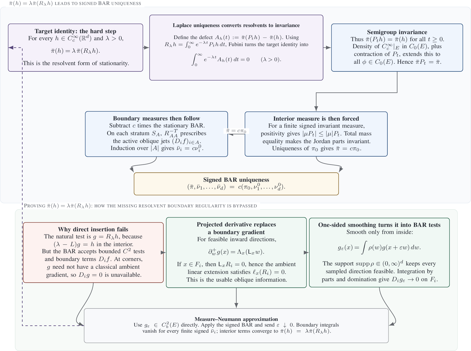
The diagram also shows why the proof first studies the nonsmooth resolvent before carrying out the smoothing. For fixed \(h\) and \(\lambda\), let \(g=R_\lambda h\). The smoothed BAR tests used later are \[g_\varepsilon(x)=\int \rho(w)g(x+\varepsilon w)\,dw, \qquad \operatorname{supp}\rho\subset(1,2)^d.\] They must approximate \(g\) in the interior equation while also satisfying an asymptotic oblique-Neumann condition on each face: \(D_i g_\varepsilon\to0\) in pairings with arbitrary finite signed measures on \(F_i\). This is why 3 proves a boundary statement for \(g\) itself before any smoothing is introduced. Although \(g\) need not be \(C^2\) on the closed orthant, its feasible one-sided derivatives exist at boundary points and factor through the active tangent projection; the resulting linear extension \(\ell_x\) satisfies \(\ell_x(R_i)=0\) on active faces, acting as an analog to the classical gradient. The one-sided convolution \(g_\varepsilon\) in 4 is then precisely designed to inherit this first-order oblique flatness in the weaker, measure-level form needed by the BAR.

3 Resolvent regularity and projected boundary derivatives↩︎

The goal of this section is to prove 3, the input that makes the measure–Neumann approximation in 4 possible. Section 4 will construct \(g_\varepsilon\in C_b^2(E)\) from \(g=R_\lambda h\) and will need three properties: \(g_\varepsilon\to g\), \((\lambda-L)g_\varepsilon\to h\), and \(D_i g_\varepsilon\to0\) on \(F_i\) after integration against arbitrary finite signed boundary measures. The first two properties come from interior smoothing and the interior resolvent equation. The third property comes from the boundary information proved here: at a boundary point, the feasible directional derivative of \(g\) factors through the active tangent projection. Combining this factorization with the identity \(\mathsf L_xR_i=0\) gives the usable oblique information \(\ell_x(R_i)=0\) on \(F_i\), which is exactly what later forces \(D_i g_\varepsilon\to0\) in boundary-measure pairings.

The proof has two ingredients. The algebraic ingredient is the nonsingularity of every active principal reflection block, which gives the explicit projection \(\mathsf L_x\). The stochastic ingredient is external: the Lipshutz–Ramanan initial-condition derivative theorem for the normalized Harrison–Reiman reflected diffusion, together with well posedness, strong-continuity property, and the synchronous Lipschitz estimate. The source-to-assumption conversion is carried out in the proof of 2, where each source hypothesis is recalled in the present orthant specialization and verified with a self-contained argument; no unlisted regularity or boundary conclusion is used.

For \(x\in E\), define \(I(x)=\{i\in J:x_i=0\},\) and put \[\begin{align} G_x=\{w\in\mathbb{R}^d:w_i\ge0\text{ for }i\in I(x)\}, \qquad H_x=\{v\in\mathbb{R}^d:v_i=0\text{ for }i\in I(x)\}. \end{align}\]

3.1 Matrix normalization and active-set projections↩︎

Normalize the reflection directions by \[\Delta=\operatorname{diag}(R_{11},\ldots,R_{dd}), \qquad \widehat R=R\Delta^{-1}, \qquad d_i=\widehat R_i=R_i/R_{ii}.\] Positive rescaling of a reflection direction only rescales its regulator and does not change the reflected path.

3.2 Regularity of SRBM↩︎

This subsection proves 2, the stochastic regularity statement used in 3. More specifically, for \(g=R_\lambda h\), we will need the reflected semigroup on \(C_0(E)\), a synchronous Lipschitz estimate for paths driven by the same Brownian motion, and a pathwise derivative with respect to the initial condition. The derivative statement is the key boundary input: at a boundary point, the initial perturbation is projected onto the active tangent space, and the active reflection directions are killed by this projection. This is the stochastic origin of the oblique flatness used in the one-sided smoothing argument.

These properties follow from the reflected-diffusion results in [25], [26]. Those results are formulated for simple polyhedral domains with normalized reflection directions. Our SRBM is the constant-coefficient orthant case of that framework, after a harmless normalization of the reflection directions. Set \[\Delta=\operatorname{diag}(R_{11},\ldots,R_{dd}),\qquad \widehat R=R\Delta^{-1},\qquad d_i=\widehat R_i=\frac{R_i}{R_{ii}} .\] Then \(\langle d_i,e_i\rangle=1\). Replacing \(R_i\) by the positive multiple \(d_i=R_i/R_{ii}\) only rescales the \(i\)th regulator coordinate and leaves the reflected path unchanged. Therefore pathwise statements proved for the normalized matrix \(\widehat R\) apply to the original BAR normalization \(R\).

2 records the regularity consequences needed for the proof of 3. Its proof first places the present SRBM into the notation of [25], [26], then verifies the relevant hypotheses under 3 –4 , and finally applies the corresponding existence, Lipschitz, and derivative results of [25], [26].

To prove 2, we use the following results for reflected diffusions in simple polyhedra [25], [26]. The general framework of [25], [26] is a more flexible version of the same reflected-diffusion equation: it allows a simple polyhedral domain, normalized face directions, and parameter-dependent coefficients. Our orthant SRBM is obtained from that framework by taking constant coefficients and normalized columns \(d_i=R_i/R_{ii}\); the only difference from the BAR notation is the harmless positive rescaling of the regulator coordinates.

Recall that [25], [26] use the following notation for the general SRBM framework, where we specialized the notation to the spatially homogeneous case. Let parameters \(\alpha\in U\), where the parameter family \(U\) is open, and let \[G=\bigcap_{i\in J}\{x:\langle x,n_i\rangle\ge c_i\}, \qquad J=\{1,\ldots,d\},\] be a minimally represented simple polyhedron with unit inward normals \(n_i\), faces \(F_i=\{x\in G:\langle x,n_i\rangle=c_i\}\), and active set \(I_G(x)=\{i:x\in F_i\}\). The normalized reflection directions satisfy \(\langle d_i(\alpha),n_i\rangle=1\). In the spatially-homogeneous-coefficient specialization we care about, the family of reflected diffusions parameterized by \(\alpha\) is written as \[Z_t^{\alpha,x} = x+b(\alpha)t+\sigma(\alpha)W_t +\sum_{i\in J}d_i(\alpha)Y_i^{\alpha,x}(t),\] where each \(Y_i^{\alpha,x}\) is continuous, nondecreasing, starts from zero, and increases only when \(Z^{\alpha,x}\in F_i\). Put \(a(\alpha)=\sigma(\alpha)\sigma(\alpha)^T\), \(N=(n_1,\ldots,n_d)\), and \(\mathcal{D}(\alpha)=(d_1(\alpha),\ldots,d_d(\alpha))\). For \(x\in G\), define \(C_G(x)=\{w:\langle w,n_i\rangle\ge0,\;i\in I_G(x)\}\) and \(H_G(x)=\{v:\langle v,n_i\rangle=0,\;i\in I_G(x)\}\). In the orthant specialization, \(G=E\), \(n_i=e_i\), \(C_G(x)=G_x\), and \(H_G(x)=H_x\). Then, [25], [26] gives the following proposition.

3.3 The probabilistic resolvent and its boundary directional derivative↩︎

The purpose of this subsection is to convert the pathwise derivative package into a boundary identity for the probabilistic resolvent. We prove only that the resolvent is a classical solution of the resolvent equation in the interior, then differentiate the time integral in feasible directions. The resulting boundary derivative is an algebraic linear functional; no classical gradient at a corner is assumed.

Fix \(\lambda>0\) and \(h\in C_c^\infty(\mathbb{R}^d)\). We regard \(h\) as a function on \(E\) and define \[\label{eq:resolvent} g(x)=R_\lambda h(x) :=\mathbb{E}\left[\int_0^\infty e^{-\lambda t}h(Z_t^x)\,dt\right].\tag{15}\]

4 One-sided smoothing and the measure–Neumann approximation↩︎

In this section we prove the resolvent insertion theorem, 5. We first prove the identity for \(h\in C_c^\infty(\mathbb{R}^d)\), regarded as a function on \(E\), by a one-sided smoothing argument. At the end of the proof, a density argument extends the identity to all \(h\in C_0(E)\). Thus, until this final density step throughout this whole section, we fix \(\lambda>0\), \(h\in C_c^\infty(\mathbb{R}^d)\), and write \(g=R_\lambda h\) as in 15 .

First we prove the insertion for smooth compactly supported \(h\), then extend it to \(C_0(E)\) by uniform approximation. A convolution supported strictly inside the orthant produces bounded \(C^2\) functions on a neighborhood of the closed state space. Integration by parts in the convolution variable proves vanishing of every oblique boundary derivative, with a bound uniform in the smoothing scale. Since the BAR is imposed on \(C_b^2(E)\), no spatial cutoff is needed in the resolvent insertion.

Now we one-sided smoothing the function \(g\). We seek a mollifier \(\rho\in C_c^\infty((1,2)^d)\) that satisfies \(\rho\ge0\) and \(\int_{\mathbb{R}^d}\rho(w)\,dw=1.\) For \(\varepsilon>0\), define \[\label{eq:one-sided-smoothing} g_\varepsilon(x)=\int_{\mathbb{R}^d}\rho(w)g(x+\varepsilon w)\,dw,\qquad h_\varepsilon(x)=\int_{\mathbb{R}^d}\rho(w)h(x+\varepsilon w)\,dw , \qquad x\in E.\tag{21}\] Because the support of \(\rho\) lies strictly inside the positive orthant, \(g_\varepsilon\) is defined and smooth on an open neighborhood of \(E\).

The next proposition is where the projected derivative information for \(g\) is used at the boundary. It proves two facts on each face \(F_i\): first, \(D_i g_\varepsilon(x)\to0\) for every \(x\in F_i\); second, the uniform bound in ?? holds. Together these imply the boundary measure convergence in ?? by dominated convergence. The pointwise limit is obtained from 5: if \(x\in F_i\) and \(w\in\operatorname{supp}\rho\subset(0,\infty)^d\), then \(w\in G_x\) and \((g(x+\varepsilon w)-g(x))/\varepsilon\to\ell_x(w)\). After integration by parts in the smoothing variable, the limit of \(D_i g_\varepsilon(x)\) becomes \(\ell_x(R_i)\), which is zero because \(\mathsf L_xR_i=0\) on active faces.

5 Proof of 2: From the resolvent identity to signed BAR uniqueness↩︎

We now complete the proof of resolvent identity criterion (2) and then complete the proof of the main Theorem (1). We first use the uniqueness of Laplace transforms to show that the signed measure that satisfies ?? is invariant for the semigroup \((P_t)\).

8 indicates that the signed-BAR interior solution \(\bar\pi\) is invariant as a signed measure for the SRBM semigroup, i.e. \(\bar\pi P_t=\bar\pi\). Then we follows the Dai-Dieker [13], using Jordan decomposition to show that \(\bar\pi\) uniquely characterizes the stationary probability distribution \(\pi_0\) of the diffusion process in the sense that \(\bar\pi=\bar\pi(E)\pi_0\).

The preceding 8 9 identifies the uniqueness of the interior measure, but an exact same assessment for boundary measure is not yet established. Therefore, by subtracting the appropriate scalar multiple of the stationary BAR vector, the remaining signed tuple has zero interior measure. Thus the only possible obstruction to the signed uniqueness of BAR solution is a purely boundary one: a collection of finite signed measures \((\eta_i)_{i=1}^d\), with \(\eta_i\) supported on \(F_i\), whose boundary pairing vanishes, i.e. \(\sum_{i=1}^d \int_{F_i} D_i f\,d\eta_i=0\) against every test function \(f\in C_b^2(E)\). If such boundary measures exist, adding them to an existing solution doesn’t change the validity of the solution. The next proposition shows that no such nontrivial boundary annihilator exists, ruling out any other signed-BAR solutions.

The proof is local on the boundary stratification and uses the nonsingular \(M\)-matrix assumption only through the invertibility of the principal reflection blocks \(R_{AA}\). On a stratum \(S_A\), the active oblique derivatives are determined by the active normal jet: \((D_i f|_{S_A})_{i\in A}=R_{AA}^T a\), where \(a=(\partial_{x_j}f|_{S_A})_{j\in A}\). Since \(R_{AA}\) is invertible, we can prescribe these oblique derivatives independently. In particular, choosing \(a=R_{AA}^{-T}e_k\,\psi\) gives \(D_i f|_{S_A}=\delta_{ik}\psi\) for \(i\in A\), and for any test function \(\psi\in C_c^\infty(S_A)\). This isolates the \(k\)-th boundary measure on \(S_A\). An induction over the codimension \(|A|\) removes all lower-stratum contributions and forces \(\eta_k|_{S_A}=0\). Since both \(A\) and \(k\in A\) are arbitrary, all boundary measures vanish.

Now, the uniqueness of Signed BAR solution in the Harrison-Reiman Class is the natural conclusion of 8-10.

Finally, we finish the proof of the signed-BAR problem.

6 Failure in the completely \(S\) class↩︎

In this section, we demonstrate a family of counterexamples in the completely \(\mathcal{S}\) class due to the singular proper active block of the relection matrix. The negative construction is summarized in 2. It has two parts: a boundary gauge identity on the singular stratum, followed by a zero-potential correction that extends the resulting centered source into the interior and adds the matching boundary occupation potential. Recall that a square matrix \(A\) is an \(S\) matrix if there exists a vector \(u>0\) such that \(Au>0\), and is completely-\(\mathcal{S}\) if every principal submatrix is an \(S\) matrix. completely-\(\mathcal{S}\) reflection matrices are the natural existence class for orthant SRBMs, but they need not have invertible principal blocks.

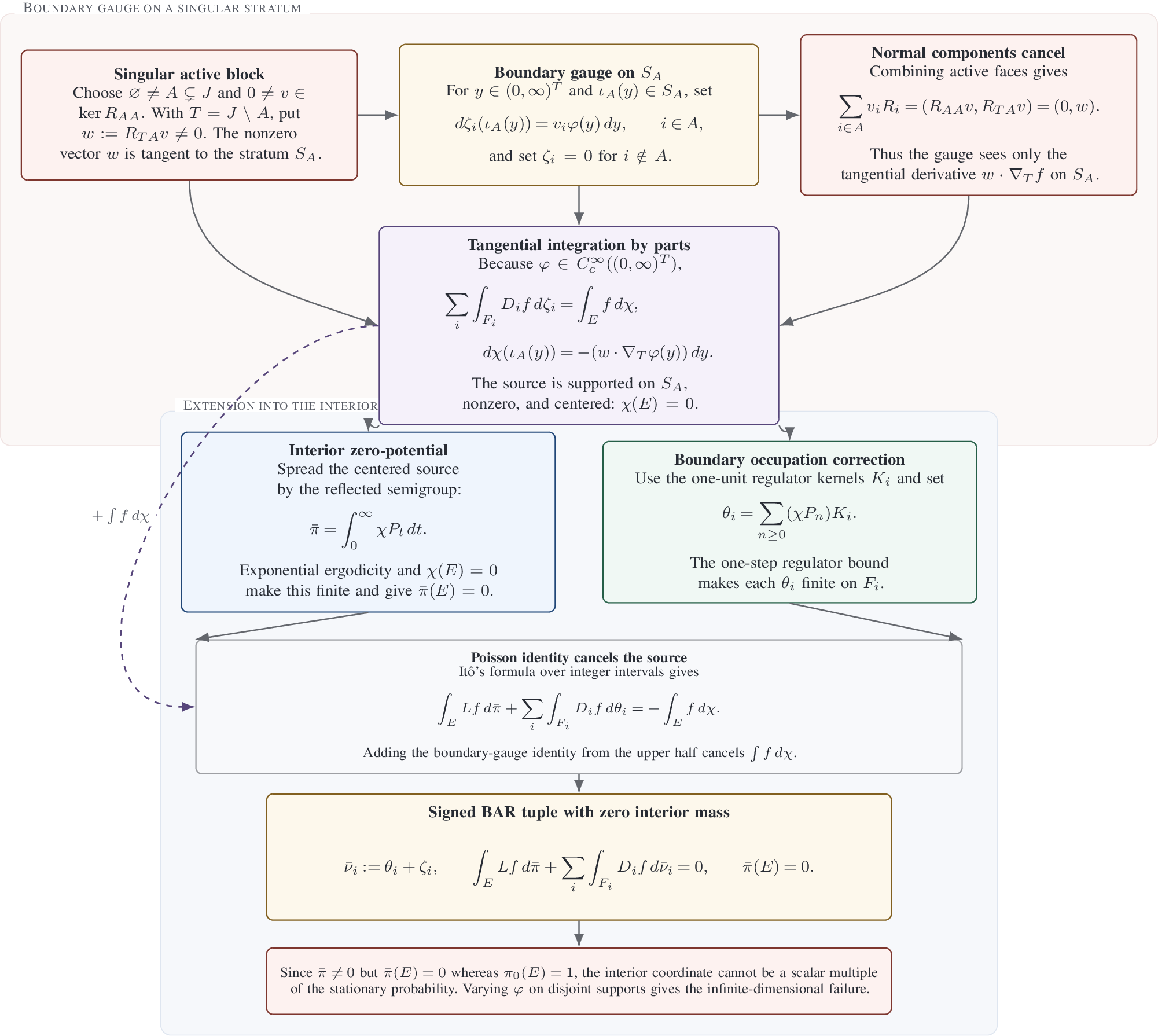
6.1 A singular-block boundary gauge↩︎

In this section, we utilize the singular proper active block of the reflection matrix to construct a nonzero null direction on that block and place a signed boundary gauge on the corresponding lower-dimensional boundary stratum. The singularity makes the active normal reflection components cancel, so the gauge leaves only a tangential derivative along the stratum. After integration by parts, this tangential derivative becomes a finite nonzero centered signed source supported on the same stratum. This source will be cancelled by the zero-potential correction in the next subsection.

Let \(J=\{1,\ldots,d\}\). For a nonempty proper set \(A\subsetneq J\), put \(T=J\setminus A\) and write \(R_{BC}\) for the submatrix with rows in \(B\) and columns in \(C\). Define the open stratum \(S_A=\{x\in E:x_i=0\text{ for }i\in A,\;x_j>0\text{ for }j\in T\}.\) We identify \(S_A\) with \((0,\infty)^T\) through the embedding \(\iota_A:(0,\infty)^T\to E\) that inserts zeros in the coordinates indexed by \(A\).

The singular block cancels the components normal to the active faces. The remaining vector \(w\) is tangent to \(S_A\), and tangential integration by parts turns the boundary gauge into the centered source \(\chi\).

6.2 Interior correction by a zero-potential↩︎

In this section, we take that centered source and spread it through the reflected Brownian semigroup by a zero potential, while also adding the matching boundary occupation potentials generated by the regulator. Under exponential ergodicity and a one-step regulator bound, these potentials are finite. Ito’s formula then shows that the zero potential contributes exactly the negative of the source created in the previous section. Adding the original boundary gauge cancels the defect and produces a genuine finite signed BAR tuple. Its interior part has total mass zero but is not the zero measure, so it cannot be a scalar multiple of the stationary distribution, whose mass is one.

Let \((P_t)_{t\ge0}\) be the transition semigroup of the SRBM, and let \(Y=(Y_1,\ldots,Y_d)\) be its regulator. For a finite signed measure \(\alpha\), we define the semigroup \((\alpha P_t)(B)=\int_E P_t(x,B)\,\alpha(dx).\) For each face define the boundary occupation kernel \[\label{eq:ce-Ki} K_i(x,B)=\mathbb{E}_x\int_0^1 \mathbf{1}_B(Z(s))\,dY_i(s),\tag{37}\] which is supported on \(F_i\).

The theorem concerns a singular proper principal block. Singularity of an arbitrary rectangular or nonprincipal submatrix does not yield the cancellation \(R_{AA}v=0\) needed in 11. Conversely, every principal block of a nonsingular \(M\)-matrix is nonsingular by 1, so this obstruction is absent from the class covered by 1.

6.3 A checkable three-dimensional family↩︎

The general obstruction is useful only if the recurrence assumptions can be verified without solving the stationary distribution. The next criterion is a direct way to do this for a broad positive-reflection subclass. A \(Z\) matrix means a matrix with nonpositive off-diagonal entries.

Set \[\label{eq:ce-R-family} R(a,b,c,d)= \begin{pmatrix} 1&1&a\\ 1&1&b\\ c&d&1 \end{pmatrix}, \qquad \Sigma=I_3, \qquad \mu=\begin{pmatrix}-11\\-7\\-11\end{pmatrix},\tag{43}\] and let \(\mathcal{P}\) be the parameter region \[\label{eq:ce-parameter-region} \begin{gather} 0<b\le\frac{11}{20}, \qquad \frac{56b+25}{60}\le a\le\frac{3b+3}{5},\qquad 0<c\le\frac{4}{25}, \qquad \frac{2}{3}\le d\le\frac{35}{46}. \end{gather}\tag{44}\] The subset obtained by making all inequalities strict is nonempty, so \(\mathcal{P}\) contains a genuine four-dimensional region.

For this entire family the algebraic source is explicit. Let \(S=\{(0,0,y):y>0\}\) and choose a nonconstant \(\phi\in C_c^\infty((0,\infty))\). Define \[\begin{align} \int_{F_1}g\,d\zeta_1 &=\int_0^\infty g(0,0,y)\phi(y)\,dy, \tag{48}\\ \int_{F_2}g\,d\zeta_2 &=-\int_0^\infty g(0,0,y)\phi(y)\,dy, \qquad \zeta_3=0. \tag{49} \end{align}\] Since \(R_1-R_2=(0,0,c-d)^T\), \[\label{eq:ce-family-source} \sum_{i=1}^3\int_{F_i}D_i f\,d\zeta_i =(d-c)\int_0^\infty\phi'(y)f(0,0,y)\,dy.\tag{50}\] Thus \[\label{eq:ce-family-chi} \chi(dx)=(d-c)\phi'(x_3)\,dx_3\, \delta_0(dx_1)\delta_0(dx_2)\tag{51}\] is nonzero and has total mass zero. Its zero potential and the corresponding boundary occupation potentials give the signed BAR counterexample.

7 Unified understanding: RI defects and boundary algebra↩︎

This section isolates resolvent insertion as the common mechanism behind both the signed BAR uniqueness theorem and the completely-\(\mathcal{S}\) obstruction. We view a signed BAR tuple through its interior coordinate and measure the failure of this coordinate to satisfy resolvent insertion by its RI defect. After quotienting out the stationary BAR direction and the pure boundary kernel, the remaining part of the BAR kernel is exactly the RI defect quotient. In the Harrison–Reiman nonsingular \(M\)-matrix class this quotient vanishes, while in the completely-\(\mathcal{S}\) singular-block regime the boundary source and its zero-potential lift produce a nonzero class in this quotient. We denote

\[\mathsf M_E=\mathcal{M}(E), \qquad \mathsf M_\partial=\prod_{i=1}^d \mathcal{M}(F_i), \qquad \mathcal{T}=C_b^2(E).\] For \((\pi,\nu)\in \mathsf M_E\times\mathsf M_\partial\), define the BAR functional \(\mathcal{A}(\pi,\nu)(f) =\int_E Lf\,d\pi+ \sum_{i=1}^d\int_{F_i}D_i f\,d\nu_i,\) for \(f\in\mathcal{T}\). Thus finite signed BAR tuples are precisely \(\ker\mathcal{A}\). Define the pure boundary operator \(\partial_R\zeta(f) =\sum_{i=1}^d\int_{F_i}D_i f\,d\zeta_i\). Since one can identify a finite signed measure \(\chi\in\mathcal{M}(E)\) with the functional \(f\mapsto\int_E f\,d\chi\) on \(\mathcal{T}\), we define the relation \(\partial_R\zeta=\chi\) by the condition that \(\sum_{i=1}^d\int_{F_i}D_i f\,d\zeta_i =\int_E f\,d\chi\) holds for all \(f\in\mathcal{T}\).

7.1 The RI-defect quotient↩︎

Let \(Z_{\rm BAR}:=\ker\mathcal{A}\) and \(\Pi_E(\pi,\nu)=\pi\), and define the space of interior coordinates of signed BAR tuples by \[\label{eq:unified-I-BAR} \mathcal{I}_{\rm BAR}:=\Pi_E Z_{\rm BAR} =\{\pi\in\mathcal{M}(E):\text{ there exists }\nu\in\mathsf M_\partial \text{ with }(\pi,\nu)\in\ker\mathcal{A}\}.\tag{58}\] For a finite signed measure \(m\in\mathcal{M}(E)\), define its resolvent-insertion defect by \[\label{eq:unified-r-defect} \mathfrak r(m)(\lambda,h) :=\int_E(\lambda R_\lambda h-h)\,dm, \qquad \lambda>0,\quad h\in C_0(E).\tag{59}\] Thus \(m\) satisfies the resolvent identity precisely when \(\mathfrak r(m)=0\). Set \(\mathcal{I}_{\rm RI}:=\mathcal{I}_{\rm BAR}\cap\ker\mathfrak r,\) and define the RI-defect quotient \(\mathcal{Q}_{\rm RI}:=\mathcal{I}_{\rm BAR}/\mathcal{I}_{\rm RI}.\) Equivalently, \(\mathcal{Q}_{\rm RI}\simeq \mathfrak r(\mathcal{I}_{\rm BAR}).\) This quotient records exactly the part of the signed BAR kernel not killed by resolvent insertion.

7.1.0.1 The positive theorem in the Harrison–Reiman Class

In the Harrison–Reiman nonsingular \(M\)-matrix setting, 5 says that every signed BAR tuple satisfies the resolvent identity. Equivalently, \(\mathfrak r(\mathcal{I}_{\rm BAR})=0\) and \(\mathcal{Q}_{\rm RI}=0.\) Then 6 reduces the quotient \(\ker\mathcal{A}/\mathbb{R} s_0\) to the pure boundary kernel. The latter is killed by 10, i.e. \(\ker\partial_R=\{0\}.\) Consequently \(\ker\mathcal{A}=\mathbb{R} s_0,\) which is the signed uniqueness conclusion of 1.

This formulation separates the two uses of active-block invertibility. First, \(R_{AA}^{-1}\) defines the active projection \[\mathsf L_Av=v-R_A R_{AA}^{-1}v_A, \qquad \mathsf L_A R_i=0, \quad i\in A.\] This is the algebraic input behind the measure–Neumann resolvent insertion. Second, \(R_{AA}^{-T}\) prescribes active oblique jets on \(S_A\). If the active normal gradient is \(a\), then \((D_i f|_{S_A})_{i\in A}=R_{AA}^T a,\) so invertibility of \(R_{AA}\) permits the choice \(a=R_{AA}^{-T}\psi\). The induction over strata in 10 uses exactly this prescription.

7.1.0.2 The completely-\(\mathcal{S}\) obstruction.

In this section, we advance our understanding of the zero potential construction as a device for cancelling the source term in the BAR but as a way of placing explicit nonzero elements into \(\mathcal{Q}_{\rm RI}\). Starting from the singular boundary gauge, one has a boundary source identity \(\partial_R \zeta = \chi .\) Thus the boundary gauge alone has BAR defect \(+\chi\). The zero potential \(Q_\chi=(U_\chi,\Theta_\chi), \text{ where } U_\chi=\int_0^\infty \chi P_t\,dt,\) is constructed so that its BAR contribution is exactly the opposite defect: \(A(Q_\chi)=-\chi .\) Therefore we have \(Q_\chi+(0,\zeta)=(U_\chi,\Theta_\chi+\zeta)\in \ker A,\) so the zero potential turns the boundary gauge into a genuine signed BAR tuple. However, this cancellation does not make the source \(\chi\) disappear. Instead, we shows that \(\chi\) reappears as the resolvent insertion defect of the interior measure \(U_\chi\): \(r(U_\chi)(\lambda,h)=-\int_E R_\lambda h\,d\chi .\) Hence, if \(\chi\neq 0\), then \(U_\chi\) cannot satisfy the resolvent insertion identity; otherwise the strong continuity of the semigroup would imply that \(\chi\) vanishes on all functions in \(C_0(E)\), forcing \(\chi=0\). Consequently, the zero potential is the mechanism that converts the singular boundary source into a concrete nonzero class. \(0\neq [U_\chi]\in Q_{\mathrm{RI}} .\) This is why the completely \(S\) counterexample is best understood as an RI defect: the boundary algebra creates the centered source \(\chi\), and the zero potential lifts that source into a genuine BAR tuple whose interior coordinate carries a nonzero resolvent insertion defect.

Suppose that \(R\) is nonsingular and that \(R_{AA}\) is singular for some nonempty proper subset \(A\subsetneq J\). Put \(T=J\setminus A\) and choose \(0\ne v\in\ker R_{AA},\) where \(w=R_{TA}v.\) Since \(R\) is nonsingular, \(w\ne0\). On \(S_A\), the local boundary symbol is \[\label{eq:unified-local-symbol} \sum_{i\in A}v_iD_i f =(R_{AA}v)\cdot\nabla_A f+(R_{TA}v)\cdot\nabla_T f.\tag{62}\] Because \(R_{AA}v=0\), only the tangential derivative \(w\cdot\nabla_T f\) remains. 11 turns this symbol calculation into a boundary source: for a compactly supported smooth density \(\phi\) on the open stratum with \(w\cdot\nabla_T\phi\not\equiv0\), it constructs boundary measures \(\zeta_i\) and a finite nonzero centered measure \(\chi\) supported on \(S_A\) such that \(\partial_R\zeta=\chi.\) Under the recurrence and regulator hypotheses of 12, 15 gives \((U\chi,\Theta\chi+\zeta)\in\ker\mathcal{A}\) and places its interior coordinate into the RI-defect quotient as \(0\ne[U\chi]\in\mathcal{Q}_{\rm RI}.\) Thus signed BAR uniqueness fails. In fact, the singular-block construction does more than produce a BAR tuple with zero total interior mass: it produces a concrete nonzero resolvent-insertion defect, \(\mathfrak r(U\chi)(\lambda,h) =-\chi(R_\lambda h).\) Therefore a global resolvent insertion theorem cannot hold in this singular-block regime once the zero-potential lift is available.

Acknowledgment↩︎

The authors would like to thank Jose Blanchet for bringing this open problem to our attention and encouraging us to pursue an AI-based solution. We are also grateful to Jose Blanchet, Yufan Chen and Wenhao Yang for their valuable feedback on this manuscript. The authors are also grateful to Bin Dong, Xiao Ma, Jiajin Li and Jianfeng Lu for their insightful discussions regarding the application of AI in mathematical proving and the formulation of our AI usage disclosure.

8 A stable example with \(g=R_\lambda h\notin C^2(E)\)↩︎

This appendix gives a concrete example in which the probabilistic resolvent \(g=R_\lambda h\) is not in \(C^2(E)\). The point is that interior smoothness and one-sided oblique flatness on open faces do not guarantee closed-domain \(C^2\) regularity at a corner. We choose a smooth nonnegative source \(h\in C_c^\infty(E^\circ)\) such that \(h\not\equiv0\) but \(h(0)=0\).

We first justify that \(g(0)>0\). Since \(h\ge0\), \(h\not\equiv0\), and \(\operatorname{supp}h\subset E^\circ\), choose \(z_\ast\in E^\circ\), \(r>0\), and \(c_h>0\) such that \(\overline{B(z_\ast,r)}\subset E^\circ\) and \(h\ge c_h\) on \(\overline{B(z_\ast,r)}\). Let \(\Gamma\) be the Harrison–Reiman Skorokhod map. On \([0,2]\), \(\Gamma\) is Lipschitz with constant \(K_\Gamma\). Define \[\gamma(t)=tz_\ast,\quad 0\le t\le1, \qquad \gamma(t)=z_\ast,\quad 1\le t\le2.\] Since \(\gamma\) stays in \(E\), \(\Gamma(\gamma)=\gamma\). For the SRBM started from zero, the free input is \(X(t)=\mu t+W(t)\). Put \(b(t)=\gamma(t)-\mu t\). Since Brownian motion has full support in \(C_0([0,2],\mathbb{R}^3)\), the event \(A=\left\{ \sup_{0\le t\le2}|W(t)-b(t)|<r/K_\Gamma \right\}\) has positive probability. On \(A\), the free input \(X\) is within \(r/K_\Gamma\) of \(\gamma\), and therefore the reflected path \(Z^0=\Gamma(X)\) is within \(r\) of \(\gamma\). Since \(\gamma(t)=z_\ast\) for \(1\le t\le2\), we have \(Z^0(t)\in B(z_\ast,r)\) throughout \([1,2]\) on \(A\). Hence \(g(0)\ge \mathbb{P}(A)c_h\int_1^2 e^{-\lambda t}\,dt > 0 .\)

On the other hand, if \(g\) were \(C^2\) up to the corner and satisfied the exact face conditions, those conditions would force \(\nabla g(0)=0\) and \(D^2g(0)=0\). The resolvent equation at the corner would then give \(0=h(0)=(\lambda-L)g(0)=\lambda g(0)\), contradicting \(g(0)>0\).

Consider \(d=3\), \(\Sigma=I_3\), and \[R= \begin{pmatrix} 1&0&-\frac{1}{2}\\ -\frac{1}{2}&1&0\\ 0&-\frac{1}{2}&1 \end{pmatrix}, \qquad R^{-1}=\frac{1}{7} \begin{pmatrix} 8&2&4\\ 4&8&2\\ 2&4&8 \end{pmatrix}\ge0 .\] Thus \(R\) is a nonsingular \(M\)-matrix. Let \(\mu=-R\mathbf{1}\); then \(R^{-1}\mu=-\mathbf{1}<0\), so the data are stable in the sense of 4 .

Choose \(h\in C_c^\infty(E^\circ)\) with \(h\ge0\) and \(h\not\equiv0\), and set \(g=R_\lambda h\) for some \(\lambda>0\). Since the Brownian input has full support on compact time intervals and the Harrison–Reiman Skorokhod map is continuous, the SRBM started from the origin has positive probability of entering a ball on which \(h>0\) and then remaining there for a nonzero time interval. Hence \(g(0)=\mathbb{E}_0\int_0^\infty e^{-\lambda t}h(Z_t)\,dt>0\). Also \(h(0)=0\), because \(h\) is supported in the interior.

Assume, for contradiction, that \(g\in C^2(E)\) in the closed-domain sense. On each open face \(F_i^\circ\), the one-sided derivative identity of 5 applies in the feasible direction \(R_i\). Since \(\mathsf L_xR_i=0\) for \(x\in F_i^\circ\), it gives \(D_i g=0\) on \(F_i^\circ\). By continuity of the first derivatives, these identities extend to the origin as \(R^T\nabla g(0)=0\). Since \(R\) is invertible, \(\nabla g(0)=0\).

Let \(H=D^2g(0)\). For \(j\ne i\), differentiating \(D_i g=R_i\cdot\nabla g=0\) in the tangential direction \(e_j\) along \(F_i^\circ\) and then letting the tangential point tend to the origin gives \(R_i^THe_j=0\). Equivalently, \(\operatorname{offdiag}(R^TH)=0\). Thus \(R^TH=\operatorname{diag}(d_1,d_2,d_3)\) for some real numbers \(d_1,d_2,d_3\), and therefore \[H=R^{-T}\operatorname{diag}(d_1,d_2,d_3) =\frac{1}{7} \begin{pmatrix} 8d_1&4d_2&2d_3\\ 2d_1&8d_2&4d_3\\ 4d_1&2d_2&8d_3 \end{pmatrix}.\] Since \(H\) is symmetric, comparison of the \((1,2)\), \((2,3)\), and \((1,3)\) entries gives \(d_1=2d_2\), \(d_2=2d_3\), and \(d_3=2d_1\). Hence \(d_1=d_2=d_3=0\), so \(H=0\).

The interior resolvent equation gives \((\lambda-L)g=h\) on \(E^\circ\). If \(g\in C^2(E)\), the left-hand side extends continuously to the origin. Since \(h(0)=0\), \(\nabla g(0)=0\), \(D^2g(0)=0\), and \(\Sigma=I_3\), this gives \(0=h(0)=(\lambda-L)g(0)=\lambda g(0)\), contradicting \(g(0)>0\). Consequently, for this stable Harrison–Reiman SRBM and this smooth compactly supported interior source, \(R_\lambda h\notin C^2(E)\).

References↩︎