Reflected Schrödinger Bridge Matching
July 03, 2026
Abstract
Recent advances in generative modeling have enabled the efficient computation of Schrödinger bridges (SB) in high-dimensional settings by leveraging partially simulation-free training methods inspired by flow matching. However, these have not covered SBs with reflecting dynamics, a useful model choice with built-in guarantees that generated samples stay in the data domain. Existing alternatives for reflected SBs instead rely on more complex training based on forward–backward SDE theory, requiring expensive higher-order derivatives and sampling entire paths during training. In this article, we introduce a partially simulation-free framework that allows reflected SBs to be trained similarly to flow matching, using a new sampling method and regression target. We demonstrate our results by coupling pairs of well-known high-dimensional image datasets. Using reflected dynamics incurs negligible additional wall-clock time during both training and inference while maintaining or slightly improving generative performance.
1 Introduction↩︎
Recent state-of-the-art progress in high-dimensional image generation has focused on iterative refinement methods such as diffusion models [@sohl2015deep; @song2019generative; @ho2020denoising; @song2020score; @dhariwal2021diffusion; @karras2022elucidating] and closely related methods such as flow matching [@lipman2023flow; @albergo2023stochastic]. In [@liu2022flow] and [@liu2022rectified], flow matching is brought closer to optimal transport theory by adding an iterative refitting step to the framework, known as rectified flows. This straightens out paths, but still offers no optimal transport (OT) guarantees. To obtain these, a more suitable approach is given by Schrödinger bridges (SB), which are a probabilistic framework for coupling two arbitrary distributions \(\pi_0, \pi_1\) that generalizes entropic optimal transport [@cuturi2013].
In theory, SBs can be seen as regularizations of an OT plan, where the OT plan is obtained in the low diffusion limit. This limit is well-established via weak convergence and large deviations theory [@mikami2004monge; @leonard2012schrodinger; @bernton2022entropic; @nilsson2025large]. In practice, SBs can be learned as diffusion SBs (DSB) [@bortoli2021diffusion] using iterative proportional fitting (IPF). A recent, more efficient alternative is iterative Markovian fitting (IMF) [@shi2023diffusion; @peluchetti2023diffusion], where models are trained in a manner very similar to rectified flows. Another, more flexible, version of this method is known as \(\alpha\)-IMF [@debortoli2024schrodinger].
Most works on SBs have focused on unconstrained reference processes. For example, [@lou2023reflected] introduce reflected forward/reverse processes to the diffusion model framework, constraining them to the unit hypercube, and showcase practical and theoretical gains for classifier-free guidance. In contrast, [@deng2024reflected] introduce a method of learning DSBs under reflected reference processes based on forward–backward SDE theory introduced in [@chen2021likelihood]. However, this method is very inefficient as it (1) requires full simulation for every training sample and (2) uses an expensive loss function which includes a divergence term.
Our goal in this paper is to take the efficient training method of (\(\alpha\)-)IMF and bring it to reflected Schrödinger bridges, specifically where the reference process is a reflected Brownian motion (RBM) on the unit hypercube.
1.0.0.1 Notation
We work on the canonical path space of continuous functions on \([0, 1]\) taking values in \(\mathbb{R}^d\), \(\Omega = C([0, 1], \mathbb{R}^d)\). Let \(X\) denote the canonical process \(X_t(\omega)\mathrel{\vcenter{:}}=\omega_t \in \mathbb{R}^d\). For a path measure \(\mathbb{P}\), denote the projection \(\mathbb{P}_t \mathrel{\vcenter{:}}= (X_t)_\# \mathbb{P}\), and similarly \(\mathbb{P}_{s, t} \mathrel{\vcenter{:}}= (X_s, X_t)_\# \mathbb{P}\). Furthermore, \(\mathbb{P}_{\mid s}(\,\cdot\mid x_s)\) is the conditional path law \(\mathbb{P}(\, \cdot \mid X_s = x_s)\), and \(\mathbb{P}_{t \mid s}\) is the conditional distribution of \(X_t\) given \(X_s\). We will assume \(\mathbb{P}_{t \mid s}\) has a density with respect to the Lebesgue measure, and abuse notation by using the same notation for the density. The conditional distribution \(\mathbb{P}_{\mid 0, 1}\) is called the bridge of \(\mathbb{P}\). For a distribution \(\Pi_{0, 1}\) on \(\mathbb{R}^d \times\mathbb{R}^d\), \(\mathbb{P}_{\mid 0, 1} \Pi_{0, 1} \mathrel{\vcenter{:}}= \int \mathbb{P}_{\mid 0, 1}(\,\cdot\mid x_0, x_1)d\Pi_{0, 1}(x_0, x_1)\) is a bridge mixture. \(\mathbb{P}^r\) denotes a path measure over \(C([0, 1], D)\) corresponding to a reflected process in the domain \(D \subseteq \mathbb{R}^d\). We call the collection of all possible bridge mixtures the reciprocal class \(\mathcal{R}(\mathbb{P})\) of \(\mathbb{P}\), and denote \(\mathcal{M}\) (\(\mathcal{M}^r\)) as the set of Markov path measures of (in \(D\) reflected) diffusion processes. When the subscript is missing, \(\nabla\) is short for \(\nabla_{x_t}\).
![Figure 1: A reflected Schrödinger bridge between two 2D distributions resembling Erwin Schrödinger (Public Domain) and the Öresund bridge [@hajotthu_oresund_bridge_2015]. The densities are derived from the pixel values of the images. Synthetic samples from one distribution are generated by evolving a reflected SDE started at a point sampled from the other.](/article/2607.03626/figs/toy-so/refl/generation_procedure.png "fig:")
2 Related work↩︎
2.1 Diffusion Schrödinger bridges and bridge matching↩︎
The first method of approximating high-dimensional SBs using deep learning was introduced by [@bortoli2021diffusion]. Their method builds on an adaptation of the Sinkhorn/IPF algorithm [@cuturi2013], which interleaves forward and backward network training procedures, iteratively retraining the models with respect to the reverse-time score of the other model, alternating between respecting either of the two marginal constraints of the SB.
[@shi2023diffusion] and [@peluchetti2023diffusion] established that DSBs (with an SDE reference process) can in fact be learned in a manner highly similar to flow matching (especially the rectified flows framework [@liu2022flow]) called DSB matching. In this method, which is presented in more detail below, one trains the score network against the drift of the reference bridge processes, obtained by the Doob \(h\)-transform [@rogers2000diffusions], where the endpoints are sampled from a coupling between the two desired marginals. The SDE with the learned drift added to the dynamics preserves the marginal distributions (under perfect training), and thus the joint distribution, of time \(0\) and \(1\) samples from this process is still a valid coupling. Thus the marginal constraints remain satisfied. The authors showed that iterating this procedure (called iterative Markovian fitting (IMF)) with the obtained coupling will converge to the Schrödinger bridge. The whole procedure can be done either backwards or forwards in time.
If the reference process used in DSB matching is a Brownian motion, the target \(h\)-transform term will be \[\label{eq:dSB-matching-Brownian-target} \frac{y-X_t}{1-t},\tag{1}\] and \(X_t\) is conditionally sampled from a Brownian bridge between \(x\) and \(y\) at time \(t \in [0,1]\), i.e. from \(\mathcal{N}((1-t)x + ty, \sigma^2 t (1-t))\). If the variance \(\sigma^2\) is taken to \(0\), this becomes \((1-t)x + ty\), and the target 1 is \(y-x\) for all \(t\), which is precisely the target for flow matching with straight conditional paths, used in [@lipman2023flow] and [@liu2022flow]. In [@liu2022rectified], it is shown that iterative training of a flow-matching vector field (in the fashion laid out for IMF) converges to a straight path interpolation between the two distributions. Despite this, these are not necessarily OT plans, while Schrödinger bridges for the appropriate reference processes are indeed true EOT plans.
2.2 Constrained generative modeling↩︎
The task of adapting diffusion models to constrained generation has been approached from various directions [@liu2023mirror; @fishman2023diffusion; @fishman2023metropolis; @christopher2024constrained]. The treatment closest to our work is that of [@lou2023reflected], who proposed a simulation-free method for learning a diffusion model where the whole process is constrained to the unit hypercube. The forward process is a reflected SDE which has the form \[\label{eq:reflected-forward-SDE} dX_t = b(t, X_t) dt + \sigma(t, X_t) dW_t + n(X_t) dL_t, \quad X_0 \sim \mu.\tag{2}\] Here, \(\{W_t\}_t\) is a Brownian motion independent of \(X_0\), \(n(x)\) is an inward pointing normal at \(x\), and \({L_t}\) is a local time for the boundary which increases only while \(X_t\) is on the boundary, exactly so that \(X_t\) stays in the domain. The time-reversal \(\{\overline{X}_t \coloneq X_{1-t}\}\) of 2 is given by [@cattiaux1988time]: \[\label{eq:reflected-reverse-SDE} d\overline{X}_t = (-b(1-t, \overline{X}_t) + \overline{g}(t, \overline{X}_t)) dt + \sigma(1-t, \overline{X}_t) d\overline{W}_t + n(\overline{X}_t) d\overline{L}_t,\tag{3}\] where \(\overline{g}(t, x) \coloneq \sigma^2(1-t) \nabla \log p(1-t, x)\) (for \(\sigma(t,x)=\sigma(t)\in \mathbb{R}\)), and \(p(t, x)\) is the density of \(\{X_t\}\). Thus, one has to learn \(\nabla \log p(1-t, x)\) in order to generate data with the reverse process 3 . The authors showed that this is possible by utilizing the Doob \(h\)-transform of the forward process 2 . In numerical experiments, they showed that this setup is greatly advantageous for mitigating oversaturation effects in the generated samples, especially under classifier-free guidance [@ho2022classifier].
[@liu2023learning] proposed a method for constrained sampling of diffusion (not Schrödinger) bridges. By means of Doob’s \(h\)-transform, a term in the drift of the (non-reflected) forward process is added, forcing the samples to a predefined support. This is used to sample discrete distributions, with compact intervals for support being another possibility.
[@caluya2021reflected] were to our knowledge the first to treat the reflected Schrödinger problem, working with the control formulation of the problem. [@deng2024reflected] then built upon this work, taking the problem to a high-dimensional generative modeling setting by incorporating and adjusting the costly forward-backward SDE framework of [@chen2021likelihood]. In the framework of [@deng2024reflected], unlike in [@lou2023reflected] and [@shi2023diffusion], the loss is not a regression of the analytic score or score-like function. This entails a greater flexibility in terms of reference processes and support domains.
3 Schrödinger bridge matching↩︎
In this section we present the framework on which the IMF2 [@shi2023diffusion; @peluchetti2023diffusion] and \(\alpha\)-IMF [@debortoli2024schrodinger] algorithms are constructed.
The goal of IMF is to approximate a Schrödinger bridge \(\mathbb{P}^*\) with respect to some reference measure \(\mathbb{Q}\) between two distributions \(\pi_0\) and \(\pi_1\), defined as \[\label{eq:schrödinger-bridge-problem} \mathbb{P}^* = \mathop{\mathrm{arg\,min}}_\mathbb{P}\left\{\operatorname{D_{KL}}(\mathbb{P}\mid\mid \mathbb{Q}) : \mathbb{P}_0 = \pi_0, \mathbb{P}_1 = \pi_1 \right\}.\tag{4}\] The reference measure \(\mathbb{Q}\) is in general the law of an SDE \[\label{eq:def-DSBM-Q-SDE} dX_t = \mu(t, X_t) dt + \sigma(t) dW_t, \quad X_0 \sim \mathbb{Q}_0.\tag{5}\] At its core, the algorithm consists of two steps – Markovian and reciprocal projection – that are alternated. We say that a measure \(\Pi\) is in the reciprocal class \(\mathcal{R}(\mathbb{Q})\) of \(\mathbb{Q}\) if \(\Pi\) is a mixture of \(\mathbb{Q}\)-bridges, i.e. \(\Pi = \Pi_{0, 1} \mathbb{Q}_{\mid 0, 1}\), and define the reciprocal projection as \(\operatorname{proj}_{\mathcal{R}(\mathbb{Q})}(\Pi) := \Pi_{0, 1} \mathbb{Q}_{\mid 0, 1}\). It can be shown that under certain conditions, the Schrödinger bridge with reference measure \(\mathbb{Q}\) is the unique path measure that is simultaneously Markovian, in the reciprocal class of \(\mathbb{Q}\), and satisfies the marginal constraints [@leonard2014survey; @shi2023diffusion].
In general, the reciprocal projection is not Markovian. Assuming some regularity, however, for a given mixture of bridges \(\Pi = \Pi_{0, 1} \mathbb{Q}_{\mid 0, 1}\) one can construct a Markov process whose marginal law at time \(t\) is equal to \(\Pi_t\). This is the Markovian projection step \(\operatorname{proj}_\mathcal{M}(\Pi)\). The resulting Markov process is the SDE \[\label{eq:nonrefl-markovian-proj} \begin{gather} dX_t = \left(\mu(t, X_t) + v^*(t, X_t)\right) dt + \sigma(t) dW_t, \quad X_0 \sim \Pi_0,\\ v^*(t, x) = \sigma^2(t) \, \mathbb{E}_{\Pi_{1 \mid t}} \left[ \nabla \log \mathbb{Q}_{1 \mid t} (X_1 \mid X_t) \;\middle|\;X_t = x \right], \end{gather}\tag{6}\] where the gradient is taken with respect to the second argument \(x_t\).
Just as the reciprocal projection breaks the Markov property, the Markovian projection breaks the bridge mixture. Instead, the algorithm preserves the marginal distributions at \(t=0\) and \(1\). Initializing the algorithm at \((\pi_0 \otimes \pi_1)\, \mathbb{Q}_{\mid 0, 1}\), if we converge to a fixed point then it is both Markov and in the reciprocal class, and is thus the Schrödinger bridge.
Diffusion Schrödinger bridge matching (DSBM) is a numerical implementation of the IMF algorithm. The main challenge is the Markovian projection step, where the drift correction \(v^*\) is approximated by a neural network and trained on a regression loss similar to diffusion model score matching [@song2019generative]. The training procedure is initialized in a mixture of bridges between the two datasets, used in the first iteration of the Markovian projection. Taking the reciprocal projection then amounts to sampling pairs at \(t=0, 1\) from this Markov process and then sampling bridges between the points in each pair. These are then stored in a cache to train the subsequent Markovian projection. Naively implementing this will result in a compounded error for \(\pi_1\), but due to the symmetry of the problem one can formulate a reverse-time Markovian projection where \(\pi_0\) is instead the target, creating a bidirectional training scheme.
Implementing IMF requires updating the training-data cache when the optimal \(v^*\) has been found and the Markovian projection has been approximated. The \(\alpha\)-IMF algorithm is an extension of IMF, where training data is instead updated continuously in an online training fashion. Here, the iterates are \[\Pi^{n+1} = (1 - \alpha) \Pi^n + \alpha \operatorname{proj}_{\mathcal{R}(\mathbb{Q})}(\operatorname{proj}_\mathcal{M}(\Pi^n)),\] which like IMF can be shown to converge to the Schrödinger bridge [@debortoli2024schrodinger]. In the corresponding implementation \(\alpha\)-DSBM, the Markovian projection optimization is not minimized fully before resuming, and the parameter \(\alpha\) is implicit in the (possibly dynamic) step size of the optimizer. The training procedure also more naturally enables the forward and backward gradient fields to be parametrized by the same network and being optimized for the forward and backward losses simultaneously. The algorithm is explained in more detail in the following section, there in its reflected version.
4 Reflected Schrödinger bridge matching↩︎
4.1 Extension of IMF↩︎
As the name suggests, RSBM is an extension of DSBM where the reference process to the SB problem 4 is a process \(\mathbb{Q}^r\) defined by the reflected SDE \[\label{eq:def-Qr-SDE} dX_t = \mu(t, X_t) dt + \sigma(t) dW_t + n(X_t) dL_t, \quad X_0 \sim \mathbb{Q}^r_0,\tag{7}\] constrained to some compact domain \(D\), on which \(\pi_0\) and \(\pi_1\) are assumed to be supported. For a formal introduction to reflected SDEs, we refer to [@pilipenko2014introduction]. In a nutshell, \(n(x)\) is the inward-pointing normal at \(x\) and the process \(L\), called the local time of \(X\) [@bjork2015pedestriansguidelocaltime], compensates the process pathwise at the boundary, ensuring it does not escape. When \(X\) is in the interior of \(D\), \(L\) is constant and the process behaves like the regular, non-reflected SDE with the same drift and diffusion coefficients.
From the PDE perspective, the density of the reflected process satisfies the same Fokker–Planck equation in \(D\) as the non-reflected, but with an additional Neumann boundary constraint. The intuition is that the flow of the density over the boundary is zero, ensuring that no mass escapes and the support remains confined to \(D\).
From a numerical point of view, the reflected SDE is estimated using Euler–Maruyama discretization where at each time step, the process is either reflected back into or projected onto the domain. As in [@lou2023reflected], we opt for reflection, with an exception for the final step which is projected.
In the IMF procedure, when the reference process is a reflected SDE, the two types of projections are analogous to the original method. The reciprocal projection is identical, i.e., \(\operatorname{proj}_{\mathcal{R}(\mathbb{Q}^r)}(\Pi) := \Pi_{0, 1} \mathbb{Q}^r_{\mid 0, 1}\). In practice, the reference process therefore needs to be on a sufficiently nice form that sampling the bridge is efficient.
The Markovian projection \(\operatorname{proj}_{\mathcal{M}^r}(\Pi)\) in the reflected case is unsurprisingly defined as the reflected SDE \[\label{eq:def-sde-of-refl-markov-proj} \begin{gather} dX_t = (\mu(t, X_t) + v^*(t, X_t)) dt + \sigma(t) dW_t + n(X_t) dL_t, \quad X_0 \sim \Pi_0, \\ v^*(t, x) = \sigma^2 (t) \, \mathbb{E}_{\Pi_{1 \mid t}} \left[ \nabla \log \mathbb{Q}^r_{1 \mid t} (X_1 \mid X_t) \;\middle|\;X_t = x \right]. \end{gather}\tag{8}\] Comparing with 6 , here the drift is adjusted by an expectation of the score of the transition density of the reflected reference process \(\mathbb{Q}^r_{1 \mid t}\). Preservation of marginal distributions holds due to the following result which is an extension of the results of the non-reflected case [@shi2023diffusion].
Proposition 1. Assume \(\sigma > 0\) and that the solutions to the involved RSDEs exist and are unique. With some regularity assumptions on \(d\Pi / d\mathbb{Q}^r\) (see Appendix 7), letting \(\mathbb{M}^* = \operatorname{proj}_{\mathcal{M}^r}(\Pi)\), the following hold:
(i) \(\mathbb{M}^*_t = \Pi_t \quad \text{for all } t \in [0, 1].\)
(ii) \(\mathbb{M}^* = \mathop{\mathrm{arg\,min}}_{\mathbb{M}\in \mathcal{M}^r} \operatorname{D_{KL}}(\Pi \mid\mid \mathbb{M}).\)
(iii) \[\begin{multlined} \label{eq:kl-div-for-markov-proj} \operatorname{D_{KL}}(\Pi \mid\mid \mathbb{M}^*) \\ = \frac{1}{2}\int_0^1 \frac{1}{\sigma^2(t)}\mathbb{E}_{\Pi_{0, t}}\left[ \left\|\sigma^2(t) \mathbb{E}_{\Pi_{1 \mid 0, t}} \left[ \nabla \log \mathbb{Q}^r_{1 \mid t}(X_1 | X_t) \mid X_0, X_t \right] - v^*(t, X_t)\right\|^2\right] dt. \end{multlined}\qquad{(1)}\]
The full proof is in Appendix 7. In summary, the major difference compared with [@shi2023diffusion] is the treatment of the Doob \(h\)-transform, which is used in retrieving the dynamics of the bridge process \(\Pi_{\mid 0}\) conditioned on the starting point. Whereas [@shi2023diffusion] produce this dynamic from the infinitesimal generator [@palmowski2002technique], we use Girsanov’s theorem to circumvent the issue of identifying the domain of the generator in the constrained regime. The remainder of the proof follows [@shi2023diffusion], adapting the tools used in their proof to the reflected setting as needed.
Under the corresponding assumptions required for IMF convergence, Proposition 1 allows the convergence argument of [@shi2023diffusion] to be carried over to the reflected setting. We are then able to state the implementation, which is identical to \(\alpha\)-DSBM except for the loss function and sampling. The main idea of DSBM is to iterate the IMF, where at each Markovian projection step, \(v^*\) in ?? is approximated with a neural network \(v_\theta\) trained on the objective of minimizing this KL divergence. The subsequent reciprocal projection is sampled from by first drawing a starting point \(X_0 \sim \Pi_0 = \pi_0\) from the training data, sampling \(X_1 \mid X_0\) from the approximate Markovian projection \[\label{eq:def-sde-of-approx-refl-markov-proj} X_1 = X_0 + \int_0^1 (\mu(t, X_t) + v_\theta(t, X_t)) dt + \int_0^1 \sigma(t) dW_t + \int_0^1 n(X_t) dL_t.\tag{9}\] with Euler–Maruyama, then sampling a bridge point \(X_t \mid X_0, X_1 \sim \mathbb{Q}^r_{t \mid 0, 1}(\, \cdot \mid X_0, X_1)\).
We follow the extension \(\alpha\)-DSBM, where only one gradient step is taken at each Markovian projection step in an online fashion. Whereas the forward and backward objectives can be alternated, we here present the case of a bidirectional model where the direction is passed together with the time \(t\) as a conditional parameter, training on the forward and backward objective simultaneously. This gives rise to the loss \[\label{eq:rsbm-bidirectional-loss} \begin{align} L(\theta ; \Pi) = \frac{1}{2} \left( L_{\to}(\theta ; \Pi) + L_{\gets}(\theta ; \Pi) \right), \quad \text{ where} \\L_{\to}(\theta ; \Pi) &= \int_0^1 \frac{1}{\sigma^2(t)}\mathbb{E}_{\Pi_{t, 1}}\left[\| \sigma^2(t) \nabla \log \mathbb{Q}^r_{1 \mid t}(X_1 \mid X_t) - v_\theta(t, X_t; \to) \|^2\right] dt, \\ L_{\gets}(\theta ; \Pi) &= \int_0^1 \frac{1}{\sigma^2(t)}\mathbb{E}_{\Pi_{0, t}}\left[\| \sigma^2(t) \nabla \log \mathbb{Q}^r_{t \mid 0}(X_t \mid X_0) - v_\theta(1-t, X_t; \gets) \|^2\right] dt.\end{align}\tag{10}\]
The \(\alpha\)-RSBM algorithm is described in 2 [@debortoli2024schrodinger]. The RSBM algorithm, corresponding to \(\alpha = 1\), can be analogously extended from DSBM [@shi2023diffusion]. In practice, an exponential moving average of the weights is tracked and used in the Euler–Maruyama sampling step in 2 to improve sample quality [@song2020improved].
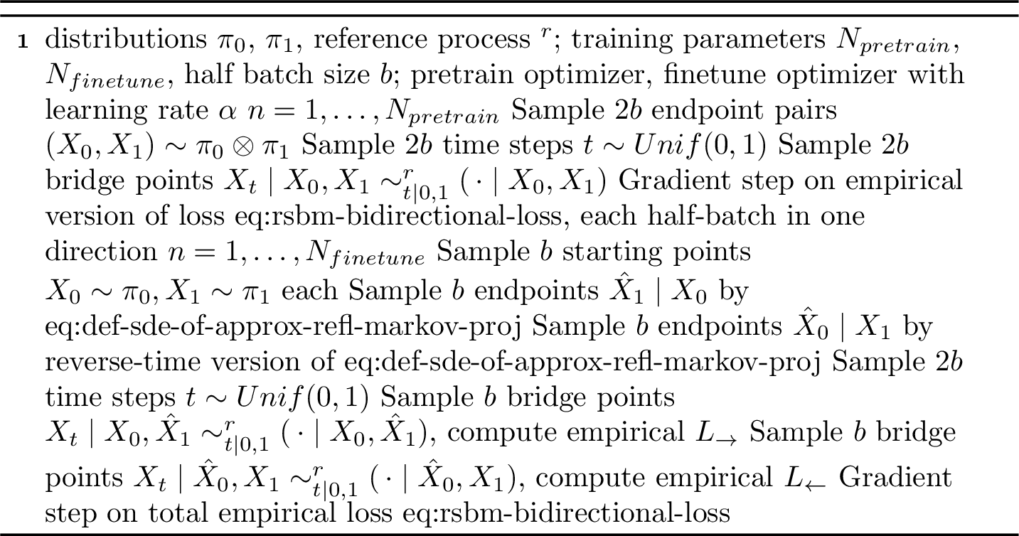
In its general form, the algorithm contains three elements that each poses a computational challenge: First, the algorithm requires sampling an endpoint \(\hat{X}_1\) of the Markovian projection 9 (and \(\hat{X}_0\), respectively) at each finetune step. Second, the same goes for sampling a bridge point from the reciprocal distribution, i.e. given the starting point \(X_0\) and the endpoint \(\hat{X}_1\) sampling from \(\mathbb{Q}^r_{t \mid 0, 1}\). Third, the loss contains the score function \(\nabla \log \mathbb{Q}^r_{1 \mid t}(x_1 \mid x_t)\) (and the reverse-time counterpart), which is in general not available in closed form. In the non-reflected case, the last two points are made tractable by letting the reference process be a scaled Brownian motion \(\sigma W\). Accordingly, we deal with these in the reflected case by restricting \(\mathbb{Q}^r\) to reflected scaled Brownian motions in the unit cube.
4.2 The score function↩︎
When \(\mathbb{Q}\) is a scaled Brownian motion with no reflection, i.e. \(\mu(t, x) = 0\) and \(\sigma(t) = \sigma\) in 5 , the transition density is a Gaussian and the score function is simply \[\nabla_{x_s} \log \mathbb{Q}_{t \mid s}(x_t \mid x_s) = \frac{x_t - x_s}{\sigma^2 \, (t - s)}.\] For a reflected Brownian motion on the unit cube, we can approximate the score cheaply. Let \(R_D: D \times \mathbb{R}^d \to D\) be the reflection operator for the domain \(D\), which computes the endpoint of the reflection of the line from \(x\) to \(y\). For \(D = [0, 1]\), \(R_{[0,1]}\) only depends on \(y\), and is given by \[\label{eq:G-reflection-operator} R_{[0,1]}(y) = \begin{cases} \phantom{(-} y & \operatorname{mod} 2, \;\text{if this is in [0, 1],} \\ (- y) & \operatorname{mod} 2, \;\text{otherwise}. \end{cases}\tag{11}\] This also holds for \(D = [0,1]^d\) for any dimension \(d\), and we denote this operator simply as \(R\). As in [@lou2023reflected], we have for the unit cube that \[\label{eq:reflected-transition-density} \mathbb{Q}^r_{t \mid s}(x_t \mid x_s) = \sum_{y_t \in \mathcal{I}(x_t)} \mathbb{Q}_{t \mid s}(y_t \mid x_s), \quad t > s,\tag{12}\] where \(\mathcal{I}(x)\) is the set of points \(y\) in \(\mathbb{R}^d\) such that \(R(y) = x\) (the inverse image of \(R\)). In practice, we truncate the infinite set \(\mathcal{I}(x)\) at a suitable distance. [@lou2023reflected] propose a hybrid approach to the reflected transition density, using the sum-of-Gaussians above for small \(\sigma\) and for larger \(\sigma\) an expansion in Laplacian eigenfunctions. We argue that sum-of-Gaussians is sufficient in our case, since we do not rely on variance-exploding dynamics.
Note that this set grows exponentially with dimension \(d\). However, when the reference process has independent components, we can instead use the factorization \[\mathbb{Q}^r_{t \mid s}(x_t \mid x_s) = \prod_{i=1}^d \mathbb{Q}^{r, i}_{t \mid s}(x_{t}^{i} \mid x_s^i) = \prod_{i=1}^d \sum_{y_t^i \in \mathcal{I}(x_t^i)} \mathbb{Q}^{i}_{t \mid s}(y_{t}^{i} \mid x_s^i).\] Thus, we can compute the Doob \(h\)-transform component-wise as \[(\nabla_{x_s} \log \mathbb{Q}^r_{t \mid s}(x_t \mid x_s))_i = \frac{d}{dx_s^i} \log \mathbb{Q}^{r, i}_{t \mid s}(x_{t}^{i} \mid x_s^i) = \frac{\sum_{y_t^i \in \mathcal{I}(x_t^i)} \frac{d}{dx_s^i} \mathbb{Q}^{i}_{t \mid s}(y_{t}^{i} \mid x_s^i)}{\mathbb{Q}^{r, i}_{t \mid s}(x_{t}^{i} \mid x_s^i)}.\]
4.3 Efficient sampling of the reflected bridge↩︎
Bridge sampling is in general not trivial either. It is possible to use Doob’s \(h\)-transform which yields an SDE with correct marginal distribution. In some cases, as with a Brownian bridge, this SDE can be solved analytically and an efficient sampling strategy can exist. Otherwise, one is left with sampling the SDE using the Euler–Maruyama method. Here, we describe an efficient sampler for the reflected Brownian bridge and prove its validity.

Proposition 2. Algorithm 3 correctly samples the RBM bridge midpoints.
Proof. Let \(W\) be a Brownian motion. Since \(\{R W_t\}_t\) has the same distribution as the reflected Brownian motion \(X\), the Markov chains \(X_0 \to X_t \to X_1\) and \(R W_0 \to R W_t \to R W_1\) have the same joint distribution, and we may work with the latter. Working conditionally on \(W_0\), we further have the Markov chain \(R W_1 \to W_1 \to W_t \to R W_t\). To sample \(W_1 \mid R W_1 = x_1\), use Bayes’ rule (also conditioning on \(W_0\)): \[\begin{align} p_{W_1 | R W_1, W_0}(y_1 | x_1, x_0) &\propto p_{R W_1 | W_1, W_0}(x_1 | y_1, x_0) p_{W_1 | W_0}(y_1 | x_0) = \delta_{R y_1}(x_1) \mathbb{Q}_{1 \mid 0}(y_1 \mid x_0), \end{align}\] where \(\delta\) is the Dirac delta. With respect to the counting measure on the set \(\mathcal{I}(x_1) = R^{-1}(x_1)\) instead, this is then proportional to \(\mathbb{Q}_{1 \mid 0}(y_1 \mid x_0)\), justifying step 1 of Algorithm 3. Step 2 is simply sampling a standard Brownian bridge to get \(W_t \mid W_0 = x_0, W_1 = y_1\). Step 3 only requires applying \(R\) to this sample. ◻
4.4 Limitations and comparison with existing reflected SB framework↩︎
As presented in the two previous subsections, we impose two limitations to make RSBM tractable: The reference process is a reflected Brownian motion, i.e. the drift \(\mu\) in 7 must be zero, and the domain D needs to be the unit cube. Not allowing drift in the reference process excludes, for example, the family of variance-preserving SDEs commonly used in diffusion modeling. This is not to say that it would not be possible, but the current theory does not support it yet. The domain restriction can be loosened if the support can mapped with a diffeomorphism to the unit cube. As [@deng2024reflected] show for a simplex domain, however, this might lead to a blow-up of the transformed true distribution in certain regions, making estimation harder.
Neither of these restrictions are needed in the reflected SB framework of [@deng2024reflected], which allows more general processes and domains. This comes at a cost of having the loss depend on the divergence of the score network, requiring two network propagations for each gradient step. The method requires SDE sampling during training, like RSBM, but in addition also relies on caching the entire path rather than just start and endpoints.
[@deng2024reflected] also bring up some limitations of their method in high dimension. They conjecture that simpler domains will still be required due to the curse of dimensionality. The high-dimensional experiments on image data are also said to be reliant on a good initialization of the score network, which is achieved by pretraining on the reflected diffusion model objective of [@lou2023reflected]. This effectively means, as for RSBM, the variance-exploding SDE is selected as reference process. For a variance-preserving reference process, [@deng2024reflected] suggest that a non-reflected variance-preserving diffusion model would be a good initialization candidate. In both cases, however, one of the marginal distributions is a noise prior (uniform or truncated Gaussian). No discussion is provided on what form of pretraining might allow for unpaired image-to-image sampling, as opposed to noise-to-image.
5 Experiments↩︎
We evaluate the proposed \(\alpha\)-RSBM model by comparing it to the non-reflected counterpart \(\alpha\)-DSBM on two image translation problems, where support is naturally constrained
to pixel values in \([0, 1]\) for grayscale or \([0, 1]^3\) for RGB images. Specifically, we approximate an SB between MNIST [@mnist] and the
first five letters (A–E, a–e) of EMNIST [@emnist], as well as between the classes cat and wild in the AFHQv2 dataset [@choi2020starganv2]. MNIST and EMNIST are both 28 \(\times\) 28 grayscale pixels. For AFHQ we downsample to a 64 \(\times\) 64 resolution.
We follow the experimental setup of [@debortoli2024schrodinger] using a reimplementation of their model. For the model, we use the U-Net implementation of [@dhariwal2021diffusion], which we augment by concatenating the directional embedding to the time embedding. The directional embedding is defined in the same way as the time embedding, namely a two-layer MLP on top of sinusoidal embeddings. These are then concatenated and used to FiLM-modulate [@perez2018FiLM] GroupNorm layers in the residual blocks. The parameters to the models and those used in training are described in more detail in Appendix 8.
For quantitative evaluation, we compare the generative performance by computing the FID between the training data of \(\Pi_1\) and synthetic samples started at the test data from \(\Pi_0\), and vice versa. One synthetic sample is generated from each starting point in the test set. MNIST contains 60,000 training samples and 10,000 test samples. For EMNIST we used the split letters, yielding
24,000 training and 4,000 test samples. In AFHQ, the cat and wild classes contained, respectively, 5065 and 4593 training images, 493 and 483 test images.
Since a Schrödinger bridge is an entropy-regularized optimal transport, a generated sample from one distribution is under moderate regularization expected to resemble the starting point from the other distribution. Qualitatively, this is observed for
both \(\alpha\)-DSBM and \(\alpha\)-RSBM as seen in 4, especially for AFHQ. Start- and end-point similarity is quantified by the (per
dimension) mean square distance (MSD) of pixel values. For AFHQ, LPIPS [@lpips] is also computed in a similar fashion to quantify this likeness with respect to closeness of AlexNet feature representations.
The comparison between \(\alpha\)-DSBM and \(\alpha\)-RSBM is presented in 1. Overall, the reflected model preserves more likeness to the source
image in all cases except in terms of LPIPS for cat \(\to\) wild. For generative quality, it is also better in all cases except wild \(\to\)
cat. As [@debortoli2024schrodinger] points out, one should not draw too strong conclusions about performance from the FID alone in these cases, as MNIST and EMNIST are
black-and-white, and because of the relatively small test sample size for AFHQ.
Some randomly chosen generated samples are shown in 4, with more examples presented in 5 and 6 in Appendix 9. There, the images with highest count of invalid entries are also presented. Comparing qualitatively clipped samples from \(\alpha\)-DSBM with samples from \(\alpha\)-RSBM for MNIST \(\leftrightarrow\) EMNIST, the models are fairly equal in terms of visual quality. We are also able to discern a stronger similarity between start and endpoint of the reflected model as indicated by the MSD.
Also for AFHQ, the models produce samples of similar quality. In many cases, the samples generated from the same starting point and with the same seed look very similar between the two models. In some cases, one model produces slightly better-looking samples than the other and vice versa, with no obvious majority. What we do want to draw attention to is the background, which seems to be more often matched by \(\alpha\)-RSBM. This is most noticeable in the samples with highest violation count, but can also be seen in some of the randomly chosen samples in 6.
More details of how the experiments were performed are laid out in Appendix 8. We wish to highlight that training \(\alpha\)-RSBM is only marginally slower than its non-reflected counterpart, with MNIST-to-EMNIST taking 32 h vs. 31.5 h (on a single 40GB A100) and AFHQ taking 109 h vs. 108 h (on four 40GB A100s). The code for reproducing the experiments is available at https://github.com/viktor765/rsbm.
We conclude this section by providing some statistics for pixel value violations, to get a sense of the scale of the problem of sampling out-of-bounds with \(\alpha\)-DSBM. The counts are in relation to the total dimension of the distributions, being number of pixels for MNIST/EMNIST and number of pixel-channel entries (three times the pixel count) for AFHQ. For the former, 100% of the generated samples had at least one pixel out-of-bounds, with an average of 46% (MNIST) and 34% (EMNIST) of pixels out of bounds. The average magnitude of a pixel violation (i.e. conditioned on the pixel being out of bounds) was around 0.002–0.003, with the maximum violation for an image averaging 0.013 (MNIST) and 0.008 (EMNIST). For AFHQ, around 2% of all pixel-channel entries were out of bounds. Around 30% of the images had more than 1% of entries out of bounds. For the threshold 5%, the frequency was around 15%. The mean magnitude of the violation was 0.02 and the mean (over images) maximum violation was 0.03. These statistics were similar for both training and test data.
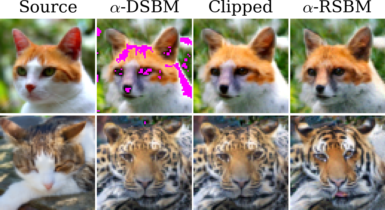
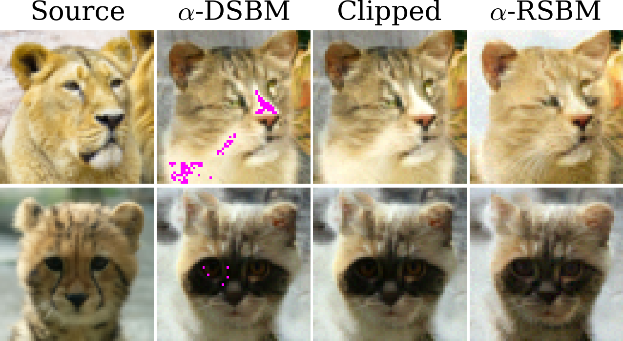
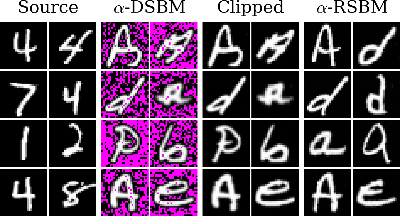
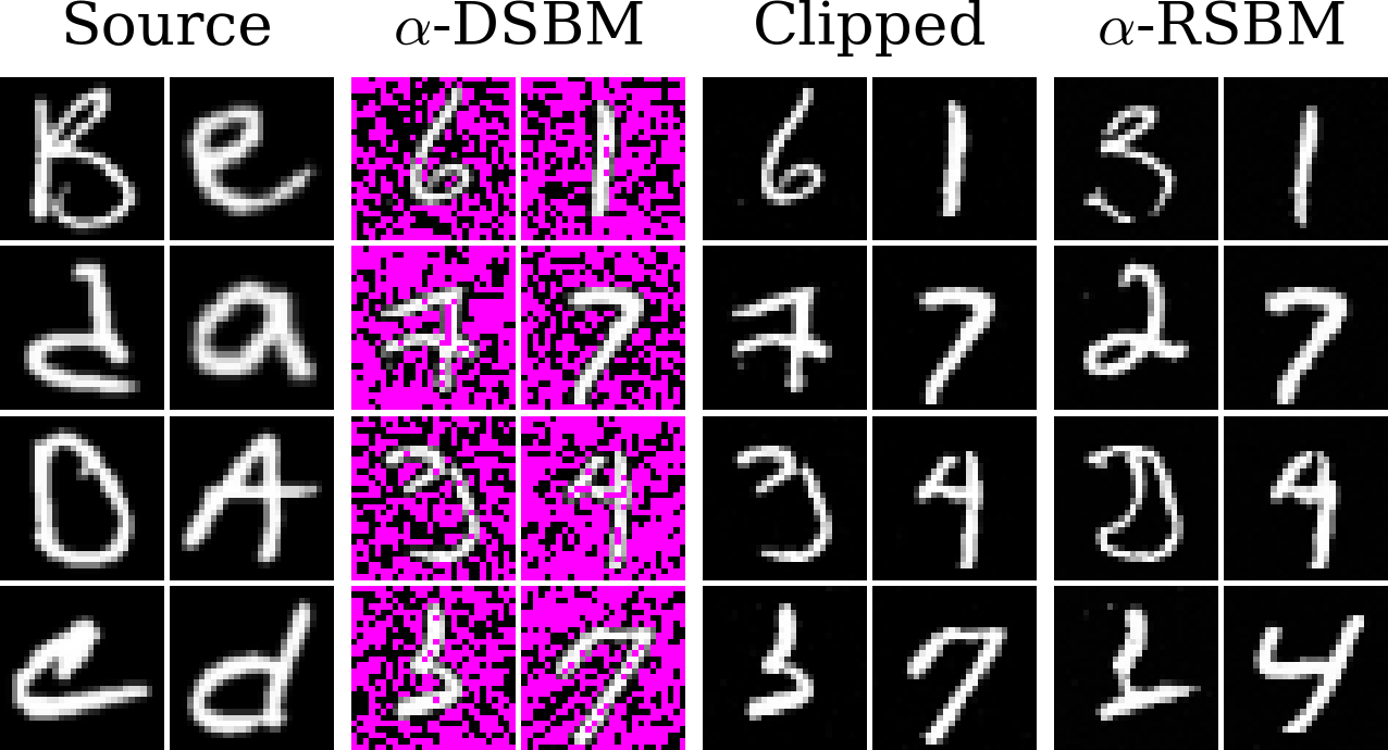
Figure 4: Transports between classes in AFHQ (\(64 \times 64\)) and MNIST/EMNIST. For each direction, the first column contains the initial (true) sample, followed by generated samples from \(\alpha\)-DSBM, clipped \(\alpha\)-DSBM and \(\alpha\)-RSBM. The out-of-bounds pixels in the \(\alpha\)-DSBM are colored magenta.
The two rows correspond to two different samples picked at random from the test data.. a — cat \(\to\) wild, b — wild \(\to\) cat, c —
MNIST \(\to\) EMNIST, d — EMNIST \(\to\) MNIST
| MNIST \(\leftrightarrow\) EMNIST | AFHQ (\(64 \times 64\)) | |||||
|---|---|---|---|---|---|---|
| 3-4 (lr)5-7 | MSD | FID | MSD | LPIPS | FID | |
| \(\Pi_0 \to \Pi_1\) | \(\alpha\)-DSBM | 0.416 | 6.41 | 0.131 | 0.239 | 27.6 |
| \(\alpha\)-RSBM | 0.356 | 5.22 | 0.084 | 0.248 | 26.1 | |
| 1-2 | \(\alpha\)-DSBM | 0.415 | 8.58 | 0.200 | 0.302 | 31.5 |
| \(\alpha\)-RSBM | 0.362 | 8.23 | 0.082 | 0.244 | 33.8 | |
6 Discussion↩︎
We have shown in this work that the IMF method of [@shi2023diffusion] can be practically applied in the setting of reflected DSBs, and that the theoretical properties are preserved. This allows learning high-dimensional DSBs on constrained domains such as \([0, 1]^d\) with the partially simulation-free framework of flow-matching and rectified flows [@liu2022flow], guaranteeing that the bounded supports of the distributions are maintained. Importantly, we demonstrate that the overhead of our method is negligible compared to [@shi2023diffusion] and [@debortoli2024schrodinger], effectively establishing our method as a cheap way of training reflected DSBs.
Extensions such as more complicated geometries and reference dynamics are left to future work, but conceptually, the main requirement is to implement efficient methods of computing the Doob \(h\)-transform term of the process, and marginally sampling its bridge processes. In the best case, these are reachable by analytical formulas and sampling schemes, but in general cases one may instead attempt to rely on neural bridge samplers and \(h\)-transform approximators [@de2021simulating; @baker2024score]. Alternatively, we may rely on solving PDEs for the \(h\)-transforms as in [@lou2023reflected].
Acknowledgements↩︎
This work was partially supported by the Wallenberg AI, Autonomous Systems and Software Program (WASP) funded by the Knut and Alice Wallenberg Foundation.
The computations were enabled by the Berzelius resource provided by the Knut and Alice Wallenberg Foundation at the National Supercomputer Centre.
7 Theory and proofs↩︎
In this appendix, we provide Proposition 1. The proof is essentially a straightforward extension of that of [@shi2023diffusion], but with a difference in treatment of the Doob h-transform.
We drop the superscript of the reflected path measures \(\mathbb{Q}^r\) and the Markov class \(\mathcal{M}^r\) from the main text. Recall the reflected SDE 7 : \[dX_t = \mu(t, X_t) dt + \sigma(t, X_t) dW_t + n(X_t) dL_t, \quad X_0 \sim \mathbb{Q}_0,\] on a domain \(D \subseteq \mathbb{R}^d\) with normal reflections.3 Assume that the SDE has a weak solution under some filtered probability space \((\Omega, \mathcal{F}, (\mathcal{F}_t)_{t\in[0,1]}, \mathbb{P})\). Let \(\mathbb{Q}\coloneq X_\# \mathbb{P}\) be its path measure.
For a given distribution \(\Pi_{0, 1}\) on \(D \times D\) we construct a path measure in the reciprocal class as \(\Pi = \mathbb{Q}_{\mid 0, 1} \Pi_{0, 1}\). Assume \(\Pi_{0, 1}\) and \(\mathbb{Q}_{0, 1}\) are equivalent, i.e., mutually absolutely continuous.
7.1 Doob’s h-transform for reflected bridge↩︎
A central notion in the Markovian projection is that Doob’s h-transform provides the means of constructing a Markov process from another Markov process which has been conditioned on ending (at time \(t=1\)) in a certain point. A typical example is that of the Brownian bridge.
More generally, our aim is to, conditioned on \(\mathcal{F}_0\), reweight the terminal distribution of \(\mathbb{Q}\) so that it becomes \(\Pi_{1 \mid 0}\) while preserving the bridge distribution \(\mathbb{Q}_{\mid 0, 1}\). [@shi2023diffusion] achieve this via the infinitesimal generator, identifying the change in drift from the generator of the process of \(\mathbb{Q}_{\mid 0}\) under the new measure [@palmowski2002technique]. To avoid characterizing the domain of the new generator in the reflected case, we instead use a Girsanov approach.
Define on \(D \times D\) \[\varphi_{1 \mid 0}(x_1 \mid x_0) \coloneq \frac{d\Pi_{1 \mid 0}}{d \mathbb{Q}_{1 \mid 0}}(x_1 \mid x_0),\] and note that \[\frac{d \Pi_{\mid 0}}{d \mathbb{Q}_{\mid 0}} = \varphi_{1 \mid 0}.\] From this we create our martingale that allows us to use Girsanov’s theorem: \[\frac{d \Pi_{1 \mid 0} \vert_{\mathcal{F}_t}}{d\mathbb{Q}_{1 \mid 0}\vert_{\mathcal{F}_t}} = \mathbb{E}_{\mathbb{Q}_{\mid 0}}\left[\frac{d \Pi_{1 \mid 0} }{d\mathbb{Q}_{1 \mid 0}} \;\middle| \; \mathcal{F}_t\right] = \mathbb{E}_{\mathbb{Q}_{1 \mid t}}[\varphi_{1 \mid 0}(X_1 \mid x_0) \mid X_t] \eqcolon \varphi_{t \mid 0}(X_t \mid x_0),\] where the second equality holds since \(\mathbb{Q}\) is Markov. Also note that \(\varphi_{0 \mid 0} = 1\).
Denoting \(d\tilde{\mathbb{P}}_{\mid 0} \coloneq \varphi_{1 \mid 0}(X_1 \mid x_0) d \mathbb{P}_{\mid 0}\), we have the following result.
Proposition 3. Assume \((t, x) \mapsto \varphi_{t \mid 0}(x \mid x_0)\) is \(C^{1, 2}\) on \([0,1] \times D\) for all \(x_0 \in D\). Assuming also that the solution exists, then \(\Pi_{\mid 0}\) is Markov, corresponding to the process \[\label{eq:sde-of-Pi-given-0} \begin{align} X_t = X_0 &+ \int_0^t \left(\mu(s, X_s) + \sigma\sigma^{\mkern-1.5mu\mathsf{T}}(s, X_s) \mathbb{E}_{\Pi_{1 \mid 0, s}}[\nabla \log \mathbb{Q}^r_{1\mid s}(X_1 \mid X_s) \mid X_0, X_s]\right) ds \\ &+ \int_0^t \sigma(s, X_s) d\widetilde{W}_s + \int_0^t n(X_s) dL_s, \end{align}\qquad{(2)}\] where \(\widetilde{W}\) is a Brownian motion under \(\tilde{\mathbb{P}}_{\mid 0}\).
Proof. Denote by \(\mathcal{A}\) the differential operator \[(\mathcal{A}f)(t, x) \coloneq \frac{\partial f(t, x)}{\partial t} + \sum_{i=1}^d \mu_i(t, x) \frac{\partial f(t, x)}{\partial x_i} + \frac{1}{2} \sum_{i=1}^d \sum_{k=1}^d a_{ik}(t, x) \frac{\partial ^2 f(t, x)}{\partial x_i \partial x_k},\] where \[a(t, x) \coloneq \sigma \sigma^{\mkern-1.5mu\mathsf{T}}(t, x).\]
Fix \(x_0\). Applying Itô’s lemma to the function \((t, x) \mapsto \varphi_{t \mid 0}(x \mid x_0)\) yields \[\begin{align} \varphi_{t \mid 0}(X_t \mid x_0) = 1 &+ \int_0^t \mathcal{A}\varphi_{s \mid 0}(X_s \mid x_0) ds + \int_0^t \nabla \varphi_{s \mid 0}(X_s \mid x_0)^{\mkern-1.5mu\mathsf{T}}\sigma(s, X_s) dW_s \\ &+ \int_0^t \nabla \varphi_{s \mid 0}(X_s \mid x_0) ^{\mkern-1.5mu\mathsf{T}}n(X_s) dL_s. \end{align}\] Rearranging the terms as \[\begin{align} \varphi_{t \mid 0}(X_t \mid x_0) - 1 - \int_0^t \nabla \varphi_{s \mid 0}(X_s &\mid x_0)^{\mkern-1.5mu\mathsf{T}}\sigma(s, X_s) dW_s \\ &= \int_0^t \mathcal{A}\varphi_{s \mid 0}(X_s \mid x_0) ds + \int_0^t \nabla \varphi_{s \mid 0}(X_s \mid x_0) ^{\mkern-1.5mu\mathsf{T}}n(X_s) dL_s, \end{align}\] since the terms on the left-hand side are continuous martingales, the right-hand side is also a continuous martingale. But this has finite variation so it must be zero almost surely [@legall2016]. Hence, \[\begin{align} d \varphi_{t \mid 0}(X_t \mid x_0) & = \nabla \varphi_{t \mid 0}(X_t \mid x_0)^{\mkern-1.5mu\mathsf{T}}\sigma(t, X_t) dW_t \\ & = \varphi_{t \mid 0}(X_t \mid x_0) \nabla \log \varphi_{t \mid 0}(X_t \mid x_0)^{\mkern-1.5mu\mathsf{T}}\sigma(t, X_t) dW_t, \end{align}\] where equivalence between \(\Pi_{\mid 0}\) and \(\mathbb{Q}_{\mid 0}\) assures \(\varphi_{t \mid 0} > 0\) a.s. By Girsanov’s theorem, \[\widetilde{W}_t \coloneq W_t - \int_0^t \sigma^{\mkern-1.5mu\mathsf{T}}(s, X_s) \nabla \log \varphi_{s \mid 0}(X_s \mid x_0) ds\] is a martingale Brownian motion on \([0, 1]\) under \(\tilde{\mathbb{P}}_{\mid 0}\). Therefore, it holds that \[dX_t = \left(\mu(t, X_t) + \sigma \sigma^{\mkern-1.5mu\mathsf{T}}(t, X_t) \nabla \log \varphi_{t \mid 0}(X_t \mid x_0) \right) dt + \sigma(t, X_t) d\widetilde{W}_t + n(X_t) dL_t.\] Finally, the computation in [@shi2023diffusion] establishing that \[\nabla \log \varphi_{t \mid 0}(x_t \mid x_0) = \mathbb{E}_{\Pi_{1\mid 0, t}}[\nabla \log \mathbb{Q}_{1 \mid t}(X_1 \mid X_t) \mid X_0 = x_0, X_t = x_t]\] follows analogously in the reflected setting, resulting in ?? . ◻
7.2 Mixture of diffusion bridges↩︎
The last ingredient needed to prove Proposition 1 is a means of getting the dynamics of the \(\Pi_0\)-mixture of diffusion bridges \(\Pi_{\mid 0}\) given by ?? . This is given by an extension of [@peluchetti2023diffusion] to reflected SDEs. For completeness, the theorem is restated here in our notation before we provide the extension to our setting.
Theorem 4 ([@peluchetti2023diffusion]). Consider the set of SDEs indexed by \(\lambda \in \Lambda\) \[\label{eq:SDEs-indexed-by-lambda} \begin{align} & dX_t^\lambda = \mu^\lambda(t, X_t^\lambda) dt + \sigma^\lambda(t, X_t^\lambda) dW_t^\lambda, \quad t \in [0, 1], \\ & X_0^\lambda \sim \mathbb{P}_0^\lambda, \end{align}\tag{13}\] corresponding to the path measures \(\{\mathbb{P}^\lambda\}_{\lambda \in \Lambda}\) and with marginal densities \(p_t^\lambda\). For a mixing \(\Psi\) on \(\Lambda\), let \(\mathbb{P}\) be obtained by taking the \(\Psi\)-mixture of 13 over \(\lambda \in \Lambda\). In particular, define the mixture marginal densities \(p_t, t \in (0,1)\), and the mixture initial measure \(\mathbb{P}_0\) by \[p_t(x) \coloneq \int_\Lambda p_t^\lambda(x) \Psi(d\lambda), \quad \mathbb{P}_0(\cdot) \coloneq \int_\Lambda \mathbb{P}_0^\lambda(\cdot) \Psi(d\lambda).\] Consider the SDE \[\label{eq:peluchetti-X95t} \begin{align} & dX_t = \mu(t, X_t) dt + \sigma(t, X_t) dW_t, \quad t \in [0, 1], \\ & \mu(t, x) \coloneq \frac{1}{p_t(x)} \int_\Lambda \mu^\lambda(t, x) p_t^\lambda(x) \Psi(d\lambda), \\ & \sigma(t, x) \coloneq \frac{1}{p_t(x)} \int_\Lambda \sigma^\lambda(t, x) p_t^\lambda(x) \Psi(d\lambda), \\ & X_0 \sim \mathbb{P}_0, \end{align}\tag{14}\] with law \(\tilde{\mathbb{P}}\). Then, under mild conditions4, \[\label{eq:Ptilde95t-equals-P95t} \tilde{\mathbb{P}}_t = \mathbb{P}_t \quad \forall t \in [0, 1].\tag{15}\]
Remark 5. In the context of this paper, the set of SDEs is indexed by \(x_0\), \(\mathbb{P}_0^{x_0} = \delta_{x_0}\) is a Dirac point mass, and mixing is done with \(\Pi_0\), whereby \(\mathbb{P}^{x_0} = \Pi_{\mid 0}(\cdot \mid X_0 = x_0)\) and \(\mathbb{P}= \Pi\).
Corollary 1. Let \(X^\lambda\) and \(X\) be the corresponding reflected processes of 13 and 14 . If \(\sigma^\lambda(t, x) = \sigma(t, x)\) is the same for all \(\lambda\), then 15 still holds.
Proof. The non-reflected case is proved by showing \(p\) and \(\tilde{p}\), the marginal densities of \(\mathbb{P}\) and \(\tilde{\mathbb{P}}\), respectively, obey the same Fokker-Planck equation. The Fokker-Planck equation for a reflected process in a domain \(D\) with normal \(n\) is the same PDE inside \(D\), but with a Neumann boundary condition [@Schuss2013]: \[(\mu p_t - \frac{1}{2}\nabla_x \cdot (\sigma \sigma^{\mkern-1.5mu\mathsf{T}}p_t) ) \cdot n = 0, \quad x \in \partial D, \; t > 0,\] using the notation \[(\nabla_x \cdot (\sigma \sigma^{\mkern-1.5mu\mathsf{T}}p_t))_i = \sum_j \partial_{x_j} \left((\sigma\sigma^{\mkern-1.5mu\mathsf{T}})_{ij} p_t\right).\] Since the Fokker-Planck equations coincide for a reflected and a non-reflected process inside \(D\), it remains to check the boundary condition: From the PDE of \(p_t\) we get the flux \[J = \mu p_t - \frac{1}{2}\nabla_x \cdot (\sigma\sigma^{\mkern-1.5mu\mathsf{T}}p_t)\] where \(\mu\) is as in 14 . The Neumann boundary condition of \(p_t\) then reads \[\begin{align} J \cdot n &= \left[ \mu p_t - \frac{1}{2}\nabla_x \cdot (\sigma\sigma^{\mkern-1.5mu\mathsf{T}}p_t) \right] \cdot n \\ &= \left[ \int_\Lambda \mu^\lambda p_t^\lambda \Psi(d\lambda) - \frac{1}{2}\nabla_x \cdot \left(\sigma\sigma^{\mkern-1.5mu\mathsf{T}}\int_\Lambda p_t^\lambda \Psi(d\lambda)\right) \right] \cdot n \\ &= \left[ \int_\Lambda \mu^\lambda p_t^\lambda \Psi(d\lambda) - \int_\Lambda \frac{1}{2}\nabla_x \cdot (\sigma\sigma^{\mkern-1.5mu\mathsf{T}}p_t^\lambda) \Psi(d\lambda) \right] \cdot n \\ &= \int_\Lambda \left[ \mu^\lambda p_t^\lambda - \frac{1}{2}\nabla_x \cdot (\sigma\sigma^{\mkern-1.5mu\mathsf{T}}p_t^\lambda) \right] \cdot n \,\Psi(d\lambda) \\ &= 0, \end{align}\] where, as in Theorem 4, we rely on the assumption that the exchange of limits going from the second to the third line holds. ◻
7.3 Proving Proposition 1↩︎
Proof. The procedure largely follows the proof of Proposition 2 in [@shi2023diffusion]. By proposition 3, \(\Pi_{\mid 0}\) is the law of the RSDE \[\begin{align} dX_t^{x_0} &= \left(\mu(t, X_t^{x_0}) + \sigma\sigma^{\mkern-1.5mu\mathsf{T}}(t, X_t^{x_0}) \, \mathbb{E}_{\Pi_{1 \mid 0, t}}[\nabla \log \mathbb{Q}^r_{1\mid t}(X_1 \mid X_t) \mid X_0=x_0, X_t = X_t^{x_0}]\right) dt \\ &\phantom{=.} + \sigma (t, X_t^{x_0}) dW_t + n(X_t^{x_0}) dL_t, \\ X_0^{x_0} &= x_0. \end{align}\]
Mixing with \(\Pi_0\) gives \(\Pi_{\mid 0} \Pi_0 = \Pi\) which by Corollary 1 has the same marginals as the RSDE with drift \[\begin{align} &\mathbb{E}_{\Pi_{0 \mid t}} \left[\mu(t, X_t) + \sigma\sigma^{\mkern-1.5mu\mathsf{T}}(t, X_t) \, \mathbb{E}_{\Pi_{1 \mid 0, t}}[\nabla \log \mathbb{Q}^r_{1\mid t}(X_1 \mid X_t) \mid X_0, X_t] \; \middle| \; X_t = x \right] \\ &= \mu(t, x) + \sigma\sigma^{\mkern-1.5mu\mathsf{T}}(t, x) \, \mathbb{E}_{\Pi_{1 \mid t}}[\nabla \log \mathbb{Q}^r_{1\mid t}(X_1 \mid X_t) \mid X_t = x] \end{align}\] and diffusion \(\sigma\), which we recognize as the coefficients in 8 of \(\mathbb{M}^*\). This establishes (i).
For (ii) and (iii), first we compute an expression of the KL divergence between \(\Pi\) and \(\mathbb{M}\in \mathcal{M}\), the path law of the solution to the RSDE \[X_t = X_0 + \int_0^t \left(\mu(s, X_s) + v^{\mathbb{M}}_s(X_s)\right) ds + \int_0^t \sigma^{\mathbb{M}}(s, X_s) dW^{\mathbb{M}}_s + \int_0^t n(X_s) dL_s, \quad X_0 \sim \mathbb{M}_0.\] Assume \(\operatorname{D_{KL}}(\Pi \mid\mid \mathbb{M}) < \infty\). Then the quadratic variation must be the same for both processes, \(\sigma^{\mathbb{M}} (\sigma^{\mathbb{M}})^{\mkern-1.5mu\mathsf{T}}= \sigma \sigma^{\mkern-1.5mu\mathsf{T}}\), almost surely. Since the local time term has bounded variation, we may use Girsanov’s theorem of [@leonard2012girsanov] to identify the change in drift going from \(\mathbb{M}\) to \(\Pi\) by \[\begin{align} \int_0^t \sigma\sigma^{\mkern-1.5mu\mathsf{T}}(s, X_s) \beta_s ds = &\int_0^t \left(\sigma\sigma^{\mkern-1.5mu\mathsf{T}}(s, X_s) \, \mathbb{E}_{\Pi_{1 \mid 0, s}}[\nabla \log \mathbb{Q}^r_{1\mid s}(X_1 \mid X_s) \mid X_0, X_s] - v_s(X_s)\right) ds. \end{align}\] The key to this step is to note that the reflection term does not change. Thus, we have \[\beta_t = \big(\sigma\sigma^{\mkern-1.5mu\mathsf{T}}(t, X_t)\big)^{-1}\left( u_t(X_0, X_t) - v_t(X_t) \right),\] with \[u_t(X_0, X_t) \coloneq \sigma\sigma^{\mkern-1.5mu\mathsf{T}}(t, X_t)\,\mathbb{E}_{\Pi_{1 \mid 0, t}}[\nabla \log \mathbb{Q}^r_{1\mid t}(X_1 \mid X_t) \mid X_0, X_t].\] Using [@leonard2012girsanov], the expression of the KL is the same form as in the unreflected case in [@shi2023diffusion]: \[\begin{align} \operatorname{D_{KL}}(\Pi \mid\mid &\mathbb{M}) - \operatorname{D_{KL}}(\Pi_0 \mid\mid \mathbb{M}_0) \\ &= \frac{1}{2} \mathbb{E}_\Pi \left[\int_0^1 (u_t(X_0, X_t) - v_t(X_t))^{\mkern-1.5mu\mathsf{T}}(\sigma\sigma^{\mkern-1.5mu\mathsf{T}}(t, X_t))^{-1} (u_t(X_0, X_t) - v_t(X_t)) dt\right] \\ &= \frac{1}{2} \int_0^1 \mathbb{E}_{\Pi_{0, t}} \left[ (u_t(X_0, X_t) - v_t(X_t))^{\mkern-1.5mu\mathsf{T}}(\sigma\sigma^{\mkern-1.5mu\mathsf{T}}(t, X_t))^{-1} (u_t(X_0, X_t) - v_t(X_t)) \right] dt, \end{align}\] where the change in order of integration is valid by Fubini’s theorem. The KL divergence is minimized when \(\mathbb{M}_0 = \Pi_0\) and, since \(\sigma \sigma^{\mkern-1.5mu\mathsf{T}}\) is positive definite, for each \(t\), \[\begin{align} v^*_t(x) &= \mathbb{E}_{\Pi_{0 \mid t}}\left[u_t(X_0, X_t) \mid X_t = x \right] \\ &= \mathbb{E}_{\Pi_{0 \mid t}}\left[\sigma\sigma^{\mkern-1.5mu\mathsf{T}}(t, X_t)\,\mathbb{E}_{\Pi_{1 \mid 0, t}}[\nabla \log \mathbb{Q}^r_{1\mid t}(X_1 \mid X_t) \mid X_0, X_t] \; \middle| \; X_t = x\right]. \end{align}\] If \(\sigma(t, x) = \sigma(t)\), this becomes \[\sigma\sigma^{\mkern-1.5mu\mathsf{T}}(t)\, \mathbb{E}_{\Pi_{1 \mid t}}[\nabla \log \mathbb{Q}^r_{1\mid t}(X_1 \mid X_t) \mid X_t = x],\] i.e. the h-transform term in the drift of 8 . ◻
8 Experiment and model details↩︎
We mimic the experimental setup of [@debortoli2024schrodinger]. As architecture we start from the U-Net implementation of [@dhariwal2021diffusion] in PyTorch [@paszke2019pytorch], extended to include conditioning on a directional embedding. Adam [@kingma2014adam] with \(\beta=(0.9, 0.999)\) is used as optimizer and gradients are clipped if exceeding unit norm.
In both experiments, we sample using an EMA model with decay rate \(0.999\), both in training in the finetuning step and for evaluation.
We used 11 reflections per dimension in the truncation of 12 .
| MNIST \(\leftrightarrow\) EMNIST | AFHQ | |
|---|---|---|
| 2-2 (l)3-3 Sample dimension | \(1 \times 28 \times 28\) | \(3 \times 64 \times 64\) |
| \(\sigma\) | 1.00 | 0.75 |
| Euler-Maruyama discretization steps | 30 | 100 |
| Model channels | 64 | 128 |
| Channel multipliers | 1, 2, 2 | 1, 2, 3, 4 |
| Number of residual blocks | 2 | 4 |
| Attention resolutions | – | 32, 16, 8 |
| Number of head channels | – | 64 |
| Dropout | 0.0 | 0.1 |
| Batch size | 256 | 128 |
| Learning rate | \(1 \times 10^{-4}\) | \(2 \times 10^{-4}\) |
| Warm-up period (linear schedule) | – | 5,000 |
| \(N_\text{pretrain}\) | 50,000 | 75,000 |
| \(N_\text{finetune}\) | 100,000 | 20,000 |
Due to a difference in implementation compared with [alg:rsbm], the batch size is doubled in finetuning.
8.1 Compute resources↩︎
The experiments were run on a HPC cluster with 40GB A100 GPUs. We ran the MNIST experiment three times in total, discovering bugs in the code in between the runs. For AFHQ, we ran the experiment twice. We had to rerun the experiment due to an incorrect model parameter configuration (attention resolutions), whereby the architecture did not match that of [@debortoli2024schrodinger].
9 Additional results↩︎
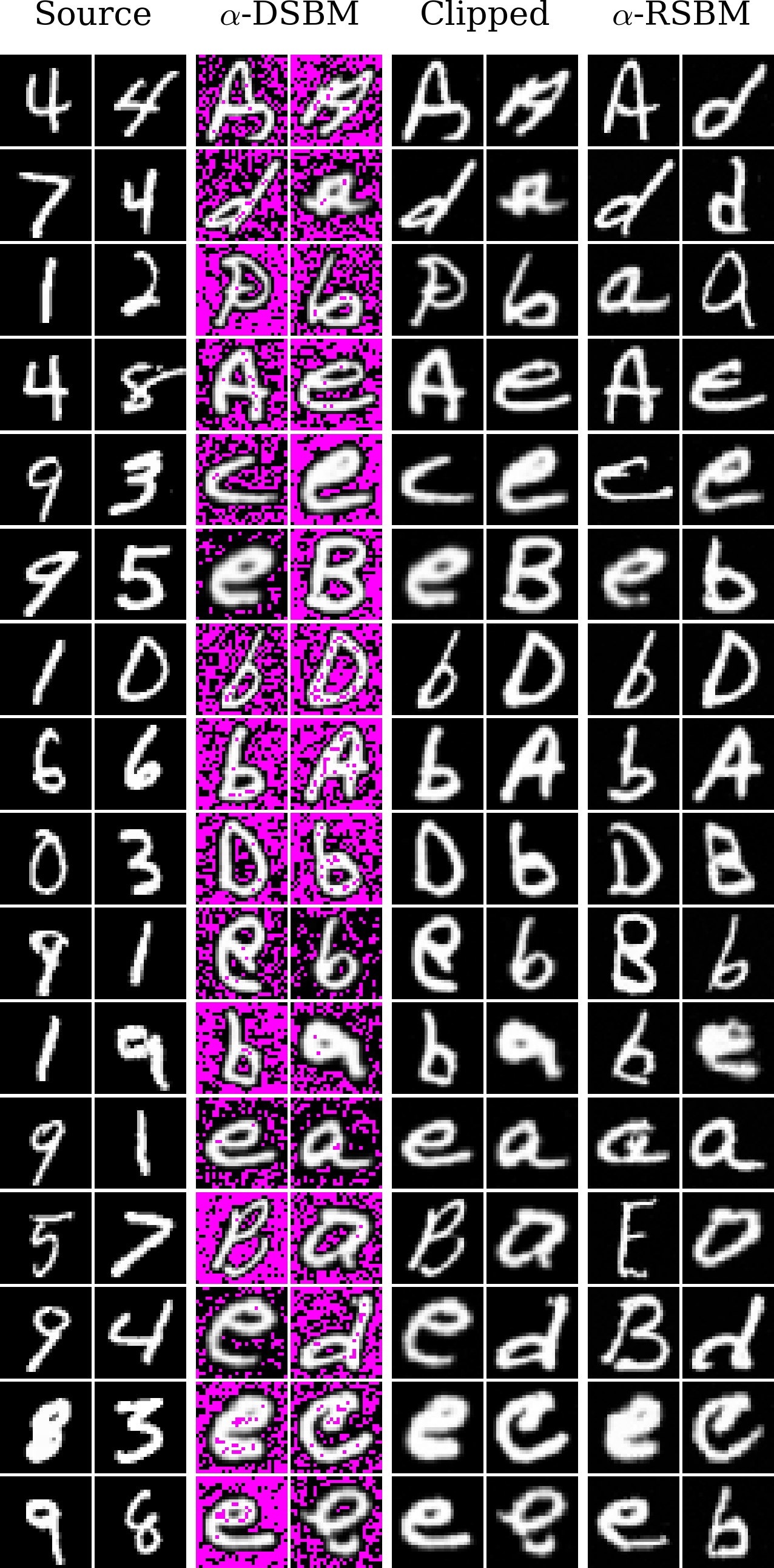
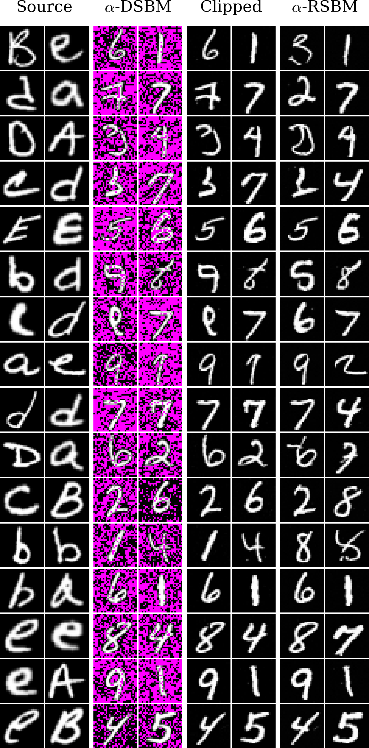
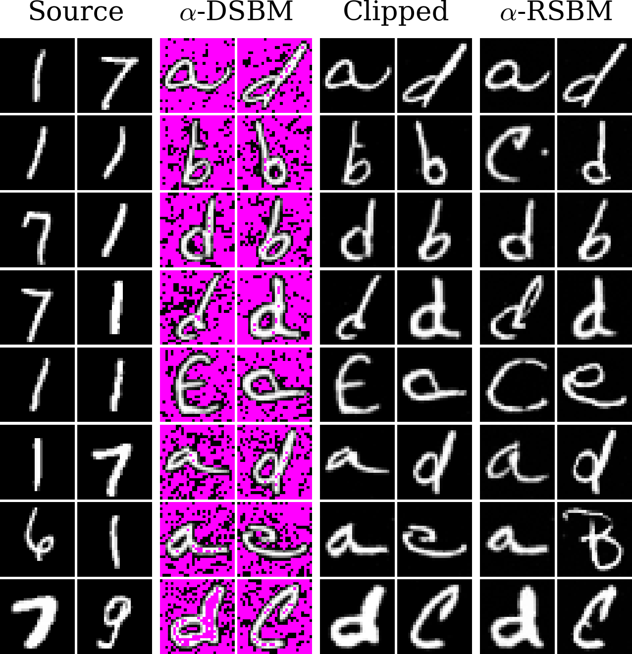
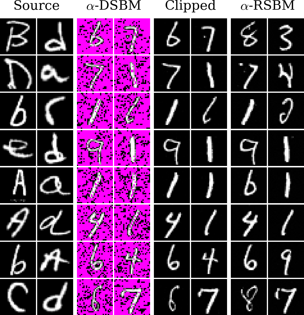
Figure 5: MNIST-to-EMNIST transfer, where (c) and (d) contains the 16 samples for which \(\alpha\)-DSBM produced highest out-of-bounds pixel count. Out-of-bounds pixels are colored in magenta.. a —
MNIST \(\to\) EMNIST, b — EMNIST \(\to\) MNIST, c — MNIST \(\to\) EMNIST, d —
EMNIST \(\to\) MNIST
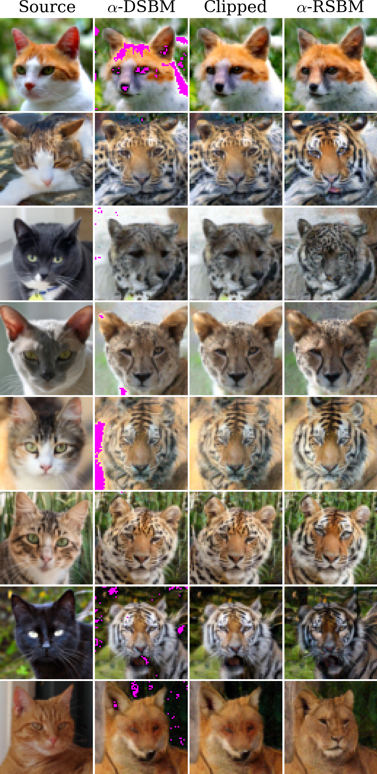
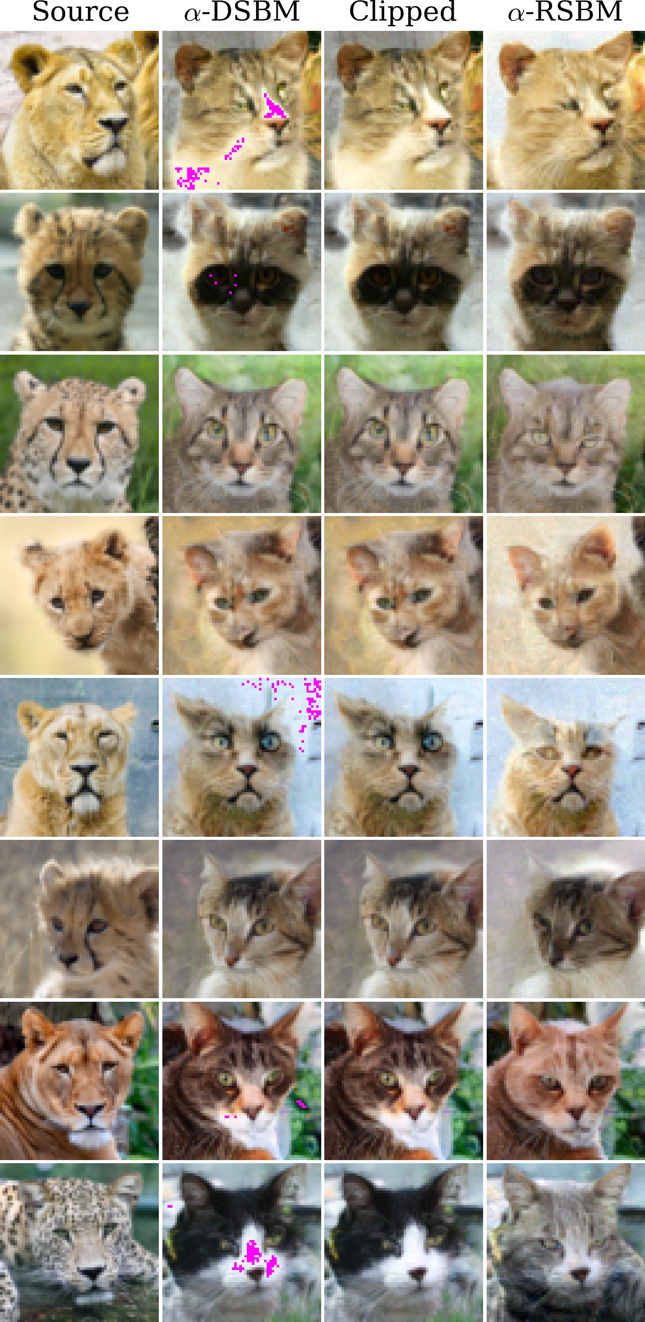
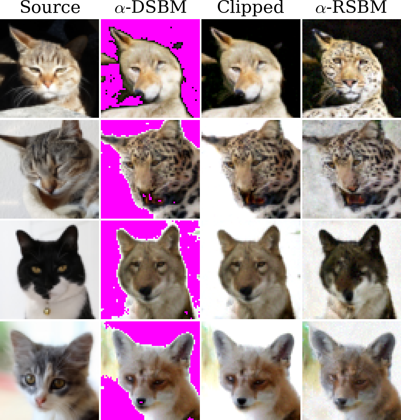
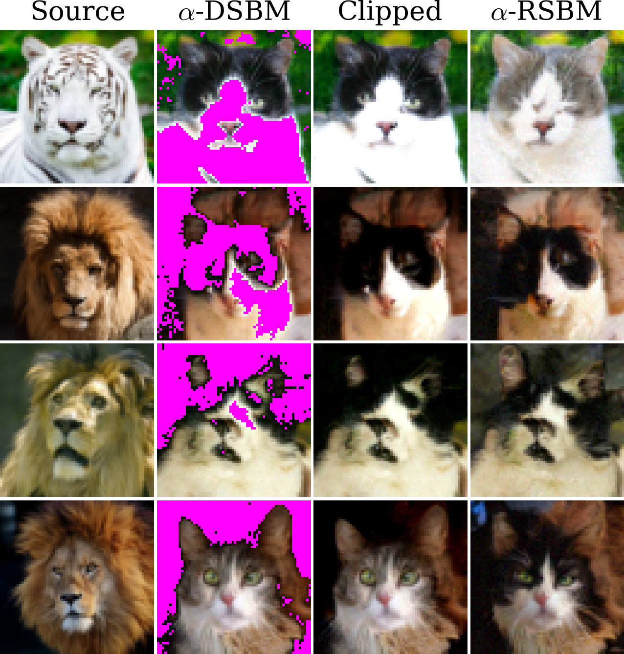
Figure 6: AFHQ (\(64 \times 64\)) transfer, where (c) and (d) contains the four samples for which \(\alpha\)-DSBM produced highest out-of-bounds pixel count. Out-of-bounds
pixels are colored in magenta.. a — cat \(\to\) wild, b — wild \(\to\) cat, c — cat \(\to\)
wild, d — wild \(\to\) cat
Equal contribution.↩︎
[@peluchetti2023diffusion] calls it the Iterated Diffusion Bridge Mixture procedure.↩︎
We here allow \(\sigma\) to be matrix-valued (such that \(\sigma\sigma^{\mkern-1.5mu\mathsf{T}}\) is positive definite) and a function of \(x\) in addition to \(t\). The dependency on \(x\) is omitted in the main text to preserve the problem symmetry when going from \(\pi_1\) to \(\pi_0\); in general an additional \(\nabla \sigma^2\) drift term appears in the reverse direction.↩︎
See [@peluchetti2023diffusion] for details.↩︎