Teacher Supervision over Representation Equivalence Classes: Why Distillation Transfers Capability Through the Output Function, Not the Features
July 03, 2026
Abstract
Knowledge distillation is usually framed as a choice of what to match in the teacher—its logits, hidden features, or sample relations—which presupposes that the teacher’s representation has absolute coordinates to match. It does not: a pretrained representation is identifiable only up to an orthogonal–and–isotropic–scaling equivalence class, so a student should learn the teacher’s equivalence class, not its features. The organizing fact is that capability is the teacher’s output function, a class invariant that factors through the quotient by the class action—so an objective recovers capability exactly when it is defined there. This makes absolute feature matching ill–posed and admissible supervision a matter of targeting class invariants (Gram structure, CKA, principal subspaces) or aligning coordinates first, unifying feature matching, relational distillation, alignment, and grafting in one geometric account. We validate on Qwen2.5 and Llama–3.1: a restoration study recovers a corrupted model’s representation (\(\mathrm{CKA}\approx0.99\)) but not its capability, and an ablation isolates the cause—output–function (logit) matching drives capability while matching hidden representations aligns geometry without restoring function. Recovery is confined to the corpus–covered region, and a graft study confirms boundary overlap predicts transplant success but is necessary, not sufficient.
Teacher Supervision over Representation
Equivalence Classes:
Why Distillation Transfers Capability Through the Output Function, Not the Features
Sang-Il Han\(^{1,2}\)
\(^1\)Korea University of Technology and Education \(^2\)Biomonster Co.
sihan@koreatech.ac.kr
April 2026
1 Introduction↩︎
Here is a puzzle. Take a corrupted language model and restore its internal representation until it almost exactly matches the teacher’s—per–layer \(\mathrm{CKA}\approx0.99\), by a label–free signal. The model stays broken: its perplexity is \(10^2\) – \(10^4\times\) worse and its top–1 agreement with the teacher is near zero. Now instead match the teacher’s output distribution and ignore the internal representation: capability returns (perplexity ratio \(\approx1.01\), top–1 \(0.98\)), even though the representation is no better aligned than before. Matching what is inside the network does not transfer what the network can do; matching what comes out of it does. Why? This paper’s answer is geometric, and it is the reason for the machinery that follows: a representation has no absolute coordinates, so “match the features” is the wrong target—capability is an invariant of the representation’s equivalence class, namely its output function, and only an objective defined on that invariant transfers it.
Before any of that machinery, it helps to fix what a model is. A network maps an input \(x\) to an output \(f(x)=W\!\bigl(H(x)\bigr)\): the input is carried to an internal representation \(H(x)\), and a reader \(W\) (the downstream weights) turns that representation into the output. Because the reader can absorb any rotation or rescaling of the representation, the same function \(f\) is computed by a whole family of pairs \((H,W)\), so a model is properly not a single \((H,W)\) but the class of all pairs computing the same output. Capability is a property of that class, not of \(H\) alone—which is exactly why matching \(H\) can leave the function untouched. The underlying fact fits in a few lines of code. A representation is just an intermediate activation, and the layer that reads it can absorb a change of its coordinate frame:
Figure 1: 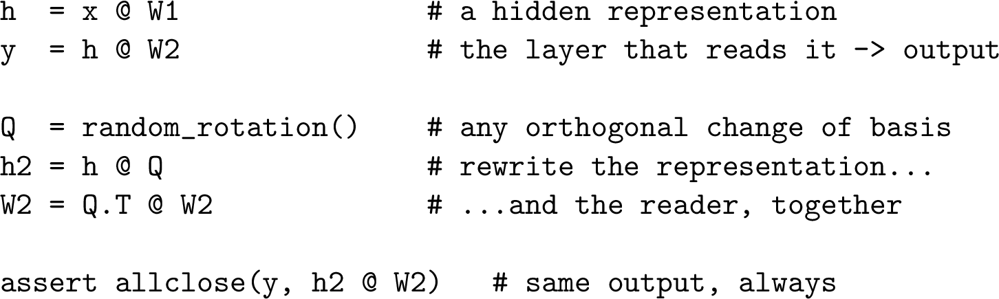 .
.
The rotated network stores completely different numbers in h2 yet computes the identical function. So the specific coordinates of h carry no information the model can use: they are an arbitrary frame, fixed only up to the
rotations (and rescalings) the next layer undoes. This is the whole premise in miniature—a feature has coordinates, the coordinates have no meaning, and only the function is determined—and it is exactly why matching a teacher’s features
basis–for–basis differs from matching its output, which is invariant to the rewrite above. The rest of the paper turns this three–line assert into a statement about equivalence classes and the quotients they form; 16 gives the same three objects this induces—orbit, fiber, quotient—as runnable code for the reader who prefers to meet them that way first.
Two words in that sentence carry the whole paper, and both have exact analogues a systems or compiler reader already owns. A feature (the vector h above) is an internal representation used by a computation—the
neural–network analogue of a compiler’s intermediate representation (IR). Just as renaming an SSA temporary changes the IR while computing the same program, \(\texttt{h}\mapsto\texttt{h @ Q}\) changes the feature while
computing the same function: the coordinates of an IR, or of a feature, are an implementation detail, not meaning. An invariant is the dual notion—the quantity that does not change under such a rewrite. This paper’s one empirical claim,
in that vocabulary, is simple: the invariant a downstream consumer can rely on is the output function, not the feature. The feature is the model’s IR, free to be recoordinatized; capability is the invariant.
Distillation and module transfer both raise the same question: in what coordinate system does the “knowledge” of a representation live? The established lines of distillation each answer a what–to–match question: logit distillation [1] matches output distributions, feature distillation [2] matches hidden activations, and relational distillation [3], [4] matches sample–to–sample structure. All three presuppose that there is a well–defined teacher quantity to match. We step back one level and question that premise. A student should reproduce the teacher’s features basis–for–basis only if those features have an absolute basis to begin with—and they do not: representations are unidentifiable up to a group of transformations. The consequence is not a new loss but a change in what teacher supervision is. The teacher is not a set of feature vectors but an equivalence class of them, and distillation is the transfer of that class (made precise in 6). We make this precise: absolute–coordinate matching is ill–posed, and transfer must target the invariants of the representation’s equivalence class, or operate in coordinates fixed by an explicit alignment. Read this way, feature matching, relational distillation, alignment–based transfer, and module grafting are not separate techniques but different points in one geometric formulation, distinguished by which part of the class structure they fix.
The distinction from prior work is sharp, and worth stating before a reader files this under “another use of CKA.” The difference is one of question, not method. Representation–similarity research [5], [6] asks how alike two representations are, and answers with a diagnostic number. We ask a different question: what transfers a capability? We therefore propose no new similarity measure and no new loss. We change the object of distillation: the representation is itself an equivalence class, and “what should we match” becomes “what is defined on the quotient the output function factors through.”
This reframing places \(\mathrm{CKA}\) precisely. It is one coordinate on the representation quotient—the coarser of the two, which forgets the reader (3). Capability instead lives on the finer, joint quotient (3), so \(\mathrm{CKA}\) is the wrong coordinate for transferring it. A similarity paper would stop at measuring it; our point is the opposite. A high \(\mathrm{CKA}\) can coexist with zero capability transfer (3), precisely because the two live on different quotients.
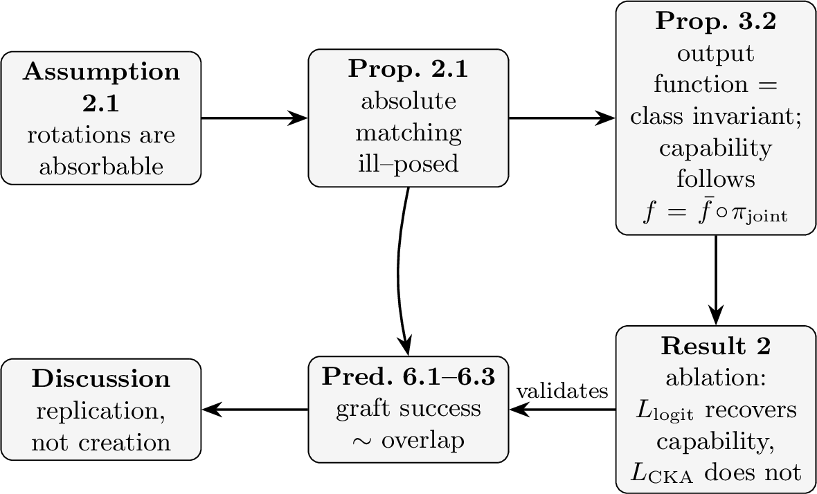
Our contribution is a single conceptual reframing of teacher supervision—from matching teacher features to transferring the teacher’s representation equivalence class—in three parts. Theory: absolute–coordinate feature matching is ill–posed (2), and the output function is the class invariant capability depends on, factoring through the quotient as \(f=\bar f\circ\pi_{\mathrm{joint}}\) (3). Loss taxonomy: this factorization sorts basis–invariant objectives and locates standard logit and feature distillation within it (5), and predicts graft success from subspace overlap (6). Experiment: restoration, ablation, and graft studies on Qwen2.5 and Llama–3.1 validate the account ([sec:experiments] [sec:graft]).
These are not three separate stories but one: teacher supervision transfers an equivalence class, and its operational core is a single distinction—a representation is an equivalence class, but capability is the output function, a class invariant (3).
1.0.0.1 Terms, fixed once.
We use four words in fixed senses. The representation is the layer activations \(\boldsymbol{H}\), defined only up to the class \([\boldsymbol{H}]\) (1); the output function \(f\) maps input to logits and is a joint–class invariant (3); capability is any scalar read off that function (perplexity, top–1)—deliberately narrow, not a claim about reasoning or generalization beyond what the logits encode; and a teacher’s knowledge, informally, means exactly that output function, the transferable content. The thesis relates them: capability rides on the output function, invariant to the representation’s coordinates. The narrowness has teeth—one–step functionals can be restored while trajectory behavior is not (7.8)—so “capability transfers” always means this output–function sense and no more.
Each experiment tests a consequence of this one statement. The restoration study (7) shows the two come apart—aligning the representation (\(\mathrm{CKA}\!\approx\!1\)) does not restore the function; restoring the function (output–function matching) does not require aligning the representation. The decoder–from–scratch result shows what follows when only the class–invariant output function is targeted: the teacher is rebuilt on whatever subspace the corpus covers. The graft study shows the same geometry governs a different operation—module transfer succeeds to the extent the boundary subspaces overlap. Read together, they say that the teacher’s transferable content is its output function (a class invariant), and “what transfers” is the part of that function one’s objective and corpus actually target.
2 Representational Unidentifiability↩︎
Fix a finite probe set \(\mathcal{X}=\{x_1,\dots,x_N\}\) of inputs, and let \(\boldsymbol{H}=\boldsymbol{H}(\mathcal{X})\in\mathbb{R}^{N\times d}\) collect the \(d\)–dimensional representations of a chosen layer, one row \(h_\ell(x_i)\) per probe. All representational quantities below—\(\boldsymbol{H}\), its Gram matrix, \(\mathrm{CKA}\), the equivalence class \([\boldsymbol{H}]\), and the quotients of 3—are defined relative to \(\mathcal{X}\): they describe what the representation encodes about this probe set. We keep \(\mathcal{X}\) fixed throughout a given comparison and suppress it in the notation when no ambiguity arises, writing \(\boldsymbol{H}\) for \(\boldsymbol{H}(\mathcal{X})\); where the choice of probes matters (the corpus–coverage results of 7) we make the dependence explicit. The pointwise object \(h_\ell(x)\in\mathbb{R}^d\) of 2 is the single–input representation; the probe matrix \(\boldsymbol{H}(\mathcal{X})\) stacks it over \(\mathcal{X}\). Throughout, \(\mathrm{O}(d)=\{\boldsymbol{Q}\in \mathbb{R}^{d\times d}:\boldsymbol{Q}^\top\boldsymbol{Q}=\boldsymbol{Q}\boldsymbol{Q}^\top=\boldsymbol{I}\}\) denotes the orthogonal group in dimension \(d\) (rotations and reflections; \(\boldsymbol{Q}^{-1}=\boldsymbol{Q}^\top\)), acting on representations by right multiplication \(h\mapsto h\boldsymbol{Q}\).
Definition 1 (Representation). Fix a probe set \(\mathcal{X}=\{x_1,\dots,x_N\}\) and a layer \(\ell\) of the network. The representation* at that layer is the matrix \[\label{eq:representation} \boldsymbol{H}=\boldsymbol{H}(\mathcal{X})\in\mathbb{R}^{N\times d}, \qquad \text{row } i \text{ of } \boldsymbol{H}\;=\; h_\ell(x_i)\in\mathbb{R}^{d},\tag{1}\] whose \(i\)th row is the layer–\(\ell\) hidden activation elicited by probe \(x_i\) (the residual–stream state after block \(\ell\), in a transformer). It is a purely empirical object: the network’s internal features sampled on \(\mathcal{X}\), and it is defined only relative to \(\mathcal{X}\)—a different probe set yields a different \(\boldsymbol{H}\). The group \(\mathcal{G}=\mathrm{O}(d)\times\mathbb{R}_+\) acts on it by \(\boldsymbol{H}\mapsto c\,\boldsymbol{H}\boldsymbol{Q}\); this action is what 2 quotients to form the equivalence class \([\boldsymbol{H}]\).*
Naming, fixed once. Throughout, \(\boldsymbol{H}\) (the layer activations) is the representation and \(\boldsymbol{W}\) (specifically \(\boldsymbol{W}_{\mathrm{in}}^{(\ell)}\)) is the reader; the function depends on the pair together, so neither alone is “the representation” (14 defends this usage against the representation–theory and computer–science readers’ objections).
A released model fixes \(\theta\), not a representation \(\boldsymbol{H}\): the shipped weights commit to one coordinate frame of the joint class, which is why coordinate–sensitive operations across independently released models need an explicit alignment (5). 12 makes this precise.
Intuitively, let \(\boldsymbol{W}_{\mathrm{in}}^{(\ell)}\) denote the first downstream operator that consumes the representation \(h_\ell\), that is, the linear map carrying one layer to the next, \[h_\ell \;\overset{\boldsymbol{W}_{\mathrm{in}}^{(\ell)}}{\longrightarrow}\;h_{\ell+1}.\] Assumption 2.1 states that any admissible coordinate change of \(h_\ell\) can be absorbed by a counter–reparametrization of \(\boldsymbol{W}_{\mathrm{in}}^{(\ell)}\), leaving the network function unchanged—rotate the features one way, rotate the weights that read them the other way, and the two cancel. (We write \(\boldsymbol{W}_{\mathrm{in}}\) for \(\boldsymbol{W}_{\mathrm{in}}^{(\ell)}\) when the layer is fixed.) This is the single premise from which the rest of the paper follows. 10 discusses when it holds exactly (a plain MLP) and when only approximately (transformers, where normalization can break it).
Assumption 1 (Absorbable reparametrization). Let the map from the layer–\(\ell\) representation to the output factor as \(\phi_{\ell{:}L}=\rho\circ\psi:\mathbb{R}^{d}\to\mathbb{R}^{V}\), where the first stage consumes the representation through a linear operator \(\boldsymbol{W}_{\mathrm{in}}\in\mathbb{R}^{d\times m}\) followed by a nonlinearity, \(\psi(h)=\tilde{\psi}(h\,\boldsymbol{W}_{\mathrm{in}})\), and any normalization between \(h\) and \(\boldsymbol{W}_{\mathrm{in}}\) commutes with \(\boldsymbol{Q}\) (exactly on the subgroup of 10). Then for \(\boldsymbol{Q}\in\mathrm{O}(d)\) and \(c\in\mathbb{R}_+\) the paired actions \(h\mapsto c\,h\boldsymbol{Q}\) and \(\boldsymbol{W}_{\mathrm{in}}\mapsto c^{-1}\boldsymbol{Q}^{\top}\boldsymbol{W}_{\mathrm{in}}\) leave the consumed product invariant, giving the absorbing identity \[\label{eq:absorb} \underbrace{\tilde{\psi}\bigl((h\boldsymbol{Q})(\boldsymbol{Q}^{\top}\boldsymbol{W}_{\mathrm{in}})\bigr)=\tilde{\psi}(h\boldsymbol{W}_{\mathrm{in}})} _{\text{(\ref{eq:absorb}a) cancellation: }\boldsymbol{Q}\boldsymbol{Q}^\top=\boldsymbol{I}} \quad\Longrightarrow\quad \underbrace{\phi_{\ell{:}L}^{\boldsymbol{Q}}(h\boldsymbol{Q})=\phi_{\ell{:}L}(h)} _{\text{(\ref{eq:absorb}b) function unchanged}},\qquad{(1)}\] so the full group acting absorbably is \(\mathcal{G}=\mathrm{O}(d)\times\mathbb{R}_+\).
A caveat on the group. The full \(\mathrm{O}(d)\) action is exact in the idealized linear/MLP case; in a real transformer, where attention \(Q/K/V\) projections, MLP projections, the residual stream, and RMSNorm gains are coupled, the exact group is the architecture–preserving subgroup of reparametrizations that every downstream operator can absorb, with the full \(\mathrm{O}(d)\) serving as the organizing approximation. Everything below is stated for \(\mathrm{O}(d)\) for clarity; the claims that matter—ill–posedness of absolute matching, invariance of the output function—hold verbatim on the subgroup, since it is a subgroup, and the appendix MLP (8) exhibits the exact case.
Here \(\phi_{\ell{:}L}^{\boldsymbol{Q}}\) denotes \(\phi_{\ell{:}L}\) with \(\boldsymbol{W}_{\mathrm{in}}\) so reparametrized; the cancellation is \((c\,h\boldsymbol{Q})(c^{-1}\boldsymbol{Q}^{\top}\boldsymbol{W}_{\mathrm{in}})=h\boldsymbol{W}_{\mathrm{in}}\), the two actions exactly inverse on the product \(h\boldsymbol{W}_{\mathrm{in}}\) that every downstream computation sees. We state ?? for \(c=1\) to keep the rotation visible; the scale factor reappears in 2 3. Conventions: \(h\in\mathbb{R}^{1\times d}\) is one row \(h_\ell(x)\) of the probe matrix, so the assumption is pointwise in \(x\) and the statement for \(\boldsymbol{H}(\mathcal{X})\) follows by stacking over rows, using row vectors throughout.
11 instantiates \(\boldsymbol{W}_{\mathrm{in}}\), \(\psi\), and \(\rho\) concretely for a transformer (the residual stream and its query/key/value projections) and for a plain MLP, where the absorbing identity is exact.
Exact vs.approximate. The absorbing identity is exact when the normalization between \(\boldsymbol{H}\) and \(\boldsymbol{W}_{\mathrm{in}}\) commutes with \(\boldsymbol{Q}\)—plain RMSNorm does; a learned per–channel gain \(\boldsymbol{\gamma}\) does so only on the subgroup it preserves, and is otherwise approximate with error set by the spread of \(\boldsymbol{\gamma}\) (10).
Status of the propositions. On the subgroup \(\mathcal{G}_0\) where 1 holds exactly, 1 2 3 are exact theorems; only the size of the equivalence class is approximate for general \(\boldsymbol{Q}\), so the qualitative claims hold as soon as \(\mathcal{G}_0\) is nontrivial, which it always is (10).
The remainder of the paper develops the consequences of 1, one per section. Once some non–identity \(\boldsymbol{Q}\) preserves the function, the representation is identified only up to \(\boldsymbol{Q}\): it is an equivalence class, not a fixed matrix (2). Matching absolute coordinates is then ill–posed (1), so only class invariants are admissible targets (3). The output function is invariant under the joint action, hence a function on the quotient (2 3). And logit distillation is singled out as the objective already defined there (5).
Definition 2 (Representation equivalence class). For \(\boldsymbol{H}\in \mathbb{R}^{N\times d}\) define \[\label{eq:class} [\boldsymbol{H}] \;=\; \bigl\{\, c\,\boldsymbol{H}\boldsymbol{Q}\;:\; \boldsymbol{Q}\in \mathrm{O}(d),\; c \in \mathbb{R}_{+} \,\bigr\},\qquad{(2)}\] the orbit of \(\boldsymbol{H}\) under right multiplication by orthogonal matrices and isotropic* positive scaling. We restrict to isotropic scaling deliberately: the invariants we use below (Gram structure, CKA) are invariant to \(\mathrm{O}(d)\) and to isotropic scaling, but not to a non–isotropic diagonal \(\boldsymbol{\Lambda}\), since \(\boldsymbol{H}\boldsymbol{\Lambda}\) changes \(\boldsymbol{H}\boldsymbol{H}^\top\). The relevant identifiability group for these invariants is therefore \(\mathrm{O}(d)\times\mathbb{R}_+\), and we define \([\boldsymbol{H}]\) to match it exactly.*
2.0.0.1 Student and teacher representations.
The distillation setting compares two representations of the same probe set \(\mathcal{X}\): the teacher’s \(\boldsymbol{H}_T=\boldsymbol{H}_T(\mathcal{X})\in\mathbb{R}^{N\times d_T}\) and the student’s \(\boldsymbol{H}_S=\boldsymbol{H}_S(\mathcal{X})\in\mathbb{R}^{N\times d_S}\), each a chosen layer’s representation evaluated on the common probes. Two conditions are needed for an absolute feature–matching loss \(\left\lVert \boldsymbol{H}_T-\boldsymbol{H}_S \right\rVert_F\) to be even well–posed as a formula, and they are worth stating because they are exactly what the equivalence–class view problematizes. First, the two must be evaluated on the same \(\mathcal{X}\), so the rows correspond (a representation is only defined relative to its probe set, 2); we assume this throughout. Second, they must share dimension, \(d_S=d_T=d\), so that the difference lives in a single space \(\mathbb{R}^{N\times d}\) and an orthogonal \(\boldsymbol{Q}\in\mathrm{O}(d)\) can act on either. We take \(d_S=d_T=d\) for 1 and the relational constructions of 3; the unequal–dimension case \(d_S\neq d_T\), where no common \(\mathbb{R}^{N\times d}\) exists and a learned map must bridge the two, is exactly what the alignment of 4 (3) handles. Even with both conditions met, the next proposition shows the loss is still ill–posed—not for lack of a shared space, but because that space carries no absolute basis.
Proposition 1 (Ill–posedness of absolute feature matching). Let \(\boldsymbol{H}_T,\boldsymbol{H}_S\in\mathbb{R}^{N\times d}\) be teacher and student representations of a common probe set \(\mathcal{X}\) (same dimension \(d\), as above), and consider the feature–matching loss \(L_{\mathrm{abs}}(\boldsymbol{H}_S) = \left\lVert \boldsymbol{H}_T - \boldsymbol{H}_S \right\rVert_F^2\). Under 1, \(L_{\mathrm{abs}}\) is not constant on the student equivalence class \([\boldsymbol{H}_S]\): there exist \(\boldsymbol{Q}\in \mathrm{O}(d)\) with \(L_{\mathrm{abs}}(\boldsymbol{H}_S \boldsymbol{Q}) \neq L_{\mathrm{abs}}(\boldsymbol{H}_S)\) while \(\boldsymbol{H}_S\boldsymbol{Q}\), once completed by the corresponding downstream reparametrization \(\boldsymbol{W}_{\mathrm{in}}\mapsto \boldsymbol{Q}^\top\boldsymbol{W}_{\mathrm{in}}\) (1), induces the same network function as \(\boldsymbol{H}_S\) with \(\boldsymbol{W}_{\mathrm{in}}\). Consequently \(L_{\mathrm{abs}}\) assigns different values to representations that are functionally equivalent once their readers are accounted for, and its minimizer is an artifact of the arbitrary representative chosen for \([\boldsymbol{H}_S]\).
Proof. Functional invariance of \(\boldsymbol{H}_S \boldsymbol{Q}\) is immediate from 1. For non–constancy, expand \[L_{\mathrm{abs}}(\boldsymbol{H}_S\boldsymbol{Q}) = \left\lVert \boldsymbol{H}_T \right\rVert_F^2 + \left\lVert \boldsymbol{H}_S \right\rVert_F^2 - 2\,\operatorname{tr}\!\bigl(\boldsymbol{Q}^\top \boldsymbol{H}_S^\top \boldsymbol{H}_T\bigr).\] Only the last term depends on \(\boldsymbol{Q}\). Let \(\boldsymbol{H}_S^\top \boldsymbol{H}_T = U\Sigma V^\top\) be a singular value decomposition with \(\Sigma \neq 0\) (generic teacher and student). The map \(\boldsymbol{Q}\mapsto \operatorname{tr}(\boldsymbol{Q}^\top U \Sigma V^\top)\) ranges over \([-\sum_i \sigma_i, \sum_i \sigma_i]\) as \(\boldsymbol{Q}\) varies over \(\mathrm{O}(d)\), taking its maximum at \(\boldsymbol{Q}= U V^\top\) (so that \(\boldsymbol{Q}^\top U\Sigma V^\top = V\Sigma V^\top \succeq 0\)). Hence it is non–constant, so \(L_{\mathrm{abs}}\) is non–constant on \([\boldsymbol{H}_S]\). ◻
2.0.0.2 The proposition, measured.
1 can be turned into a direct measurement. Take a real teacher representation \(\boldsymbol{H}\) (Qwen2.5–0.5B, layer \(12\), \(d=896\)) and apply an orthogonal reparametrization \(\boldsymbol{H}\mapsto\boldsymbol{H}\boldsymbol{Q}\), interpolating \(\boldsymbol{Q}\) from the identity to a random rotation. The rotation is function–preserving in the sense of 2: a compensating downstream reparametrization \(\phi^{\boldsymbol{Q}}\) exists for which \(f^{\boldsymbol{Q}}=f\). The table evaluates the distillation losses only on the two representatives \(\boldsymbol{H}\) and \(\boldsymbol{H}\boldsymbol{Q}\), which is exactly what a representational objective sees. We compare three losses on the pair \((\boldsymbol{H},\boldsymbol{H}\boldsymbol{Q})\): absolute feature matching \(\left\lVert \boldsymbol{H}-\boldsymbol{H}\boldsymbol{Q} \right\rVert_F^2\), the CKA loss \(1-\mathrm{CKA}\), and the normalized–Gram loss \(L_{\mathrm{rel}}\). The two representatives are the same information in rotated coordinates, yet 1 shows the feature–matching loss growing without bound (to \(\sim\!7\times10^5\) at a full rotation) while \(1-\mathrm{CKA}\) and \(L_{\mathrm{rel}}\) stay at \(0\) to machine precision for every rotation. Absolute matching penalizes a change that alters nothing about the function; the basis–invariant objectives are exactly blind to it. This is 1 as an experimental fact; its training–level counterpart appears in 7, where optimizing \(L_{\mathrm{cka}}\) to \(\mathrm{CKA}\!\to\!1\) still leaves the function destroyed (3)—1 is the static form, the ablation the dynamic one.
This also settles a natural worry: is “\(\mathrm{CKA}\!\approx\!1\) yet capability zero” an artifact of CKA specifically—a known insensitivity of CKA to small–eigenvalue directions—rather than a fact about representation matching? It is not. The failure is not a property of CKA as a measure but of basis invariance as a class of objective. 1 is proved for any loss that is constant on \([\boldsymbol{H}_S]\), and 1 exhibits the same blindness for \(L_{\mathrm{rel}}\) (a normalized–Gram, kernel–free objective) as for CKA: both stay at \(0\) under a full function–preserving rotation. Any measure fine enough to distinguish the two representatives would, by definition, no longer be basis–invariant—and would then penalize the very rotations that leave the function unchanged, i.e.behave like absolute matching and fail for the opposite reason. The gap between \(\mathrm{CKA}\!\to\!1\) and capability is therefore not a resolution limit of one similarity index but the structural fact that the output–selecting representative is quotiented away by every basis–invariant objective.
| rotation \(t\) | \(\norm{\HH-\HH\QQ}_F^2/N\) | \(1-\CKA\) | \(L_{\mathrm{rel}}\) |
|---|---|---|---|
| 0.00 | \(0\) | \(0\) | \(0\) |
| 0.10 | \(1.1\times10^4\) | \(0\) | \(0\) |
| 0.25 | \(6.9\times10^4\) | \(0\) | \(0\) |
| 0.50 | \(2.5\times10^5\) | \(0\) | \(0\) |
| 0.75 | \(4.9\times10^5\) | \(0\) | \(0\) |
| 1.00 | \(7.0\times10^5\) | \(0\) | \(0\) |
3 Admissible Targets: Equivalence–Class Invariants↩︎
Before exhibiting specific quantities, we say precisely what it means for one to be an invariant.
Definition 3 (Class invariant). A map \(q\) defined on representations is a (\(\mathcal{G}\)–)invariant* if it is constant on each equivalence class, i.e. \[\label{eq:invariant} q(c\,\boldsymbol{H}\boldsymbol{Q})=q(\boldsymbol{H})\qquad\text{for all }\boldsymbol{Q}\in\mathrm{O}(d),\;c\in\mathbb{R}_+,\tag{2}\] equivalently if \(q\) factors through the quotient onto \(\mathbb{R}^{N\times d}/\mathcal{G}\) (the representation quotient defined in 4 below) as a well–defined function of the class. A function of two representations is an invariant if it is constant under the action applied to either argument separately. An invariant is thus a well–defined function of the class \([\boldsymbol{H}]\), not of the representative; it is exactly the kind of quantity a distillation objective may legitimately target, since by 1 anything not of this form depends on the arbitrary basis.*
We now exhibit three invariants: the Gram structure, \(\mathrm{CKA}\), and the principal–angle spectrum.
The first invariant is relational. The (uncentered) Gram matrix is \(\boldsymbol{K}= \boldsymbol{H}\boldsymbol{H}^\top \in \mathbb{R}^{N\times N}\), with centered version \(\widehat{\boldsymbol{K}} = \boldsymbol{C}\boldsymbol{K}\boldsymbol{C}\) where \(\boldsymbol{C} = \boldsymbol{I} - \tfrac1N \boldsymbol{1}\boldsymbol{1}^\top\) (\(\boldsymbol{1}\in\mathbb{R}^{N}\) the all–ones vector, \(\boldsymbol{I}\) the \(N\times N\) identity). It records inter–sample geometry, and is orthogonally invariant:
Lemma 1 (Orthogonal invariance of the Gram structure). For all \(\boldsymbol{Q}\in \mathrm{O}(d)\), \((\boldsymbol{H}\boldsymbol{Q})(\boldsymbol{H}\boldsymbol{Q})^\top = \boldsymbol{H}\boldsymbol{H}^\top\). Thus \(\boldsymbol{K}\) and \(\widehat{\boldsymbol{K}}\) are invariant under the orthogonal part of \([\boldsymbol{H}]\).
Proof. \((\boldsymbol{H}\boldsymbol{Q})(\boldsymbol{H}\boldsymbol{Q})^\top = \boldsymbol{H}\boldsymbol{Q}\boldsymbol{Q}^\top\boldsymbol{H}^\top = \boldsymbol{H}\boldsymbol{H}^\top\) since \(\boldsymbol{Q}\boldsymbol{Q}^\top = \boldsymbol{I}\). ◻
The Gram matrix records inter–sample geometry (distances and angles), which is exactly the information the representation carries about the probe set, stripped of the arbitrary coordinate frame.
Definition 4 (Centered Kernel Alignment). For representations \(\boldsymbol{H}_A,\boldsymbol{H}_B\) with centered Gram matrices \(\widehat{\boldsymbol{K}}_A,\widehat{\boldsymbol{K}}_B\), and writing \(\left\langle A,\, B \right\rangle_F=\operatorname{tr}(A^\top B)\) for the Frobenius inner product (with \(\left\lVert A \right\rVert_F=\left\langle A,\, A \right\rangle_F^{1/2}\)), \[\label{eq:cka} \mathrm{CKA}(\boldsymbol{H}_A,\boldsymbol{H}_B) \;=\; \frac{\left\langle \widehat{\boldsymbol{K}}_A,\, \widehat{\boldsymbol{K}}_B \right\rangle_F}{\left\lVert \widehat{\boldsymbol{K}}_A \right\rVert_F\,\left\lVert \widehat{\boldsymbol{K}}_B \right\rVert_F}\;\in[0,1].\qquad{(3)}\] Linear CKA was introduced by [5] as a representation similarity index invariant to orthogonal transformation and isotropic scaling, building on kernel–target alignment [7] and centered alignment [8]; it is a normalized Hilbert–Schmidt independence criterion [9].
Corollary 1. \(\mathrm{CKA}\) is invariant under orthogonal transformation and isotropic scaling of either argument, and therefore is a well–defined similarity on equivalence classes \([\boldsymbol{H}_A],[\boldsymbol{H}_B]\).
Proof. Orthogonal invariance follows from 1. Isotropic scaling \(\boldsymbol{H}\mapsto c\boldsymbol{H}\) scales \(\widehat{\boldsymbol{K}}\) by \(c^2\), which cancels in the normalized ratio. ◻
A third invariant measures shared subspace. If \(\boldsymbol{H}_A,\boldsymbol{H}_B\) have orthonormal column bases \(\boldsymbol{U}_A,\boldsymbol{U}_B\) and \(k=\min(\operatorname{rank}\boldsymbol{H}_A,\operatorname{rank}\boldsymbol{H}_B)\), the principal angles \(\theta_1\le\dots\le\theta_k\) satisfy \(\cos\theta_i = \sigma_i(\boldsymbol{U}_A^\top \boldsymbol{U}_B)\) (the \(i\)th singular value of \(\boldsymbol{U}_A^\top\boldsymbol{U}_B\)), and the effective shared dimension is \(k_{\mathrm{eff}} = \sum_{i=1}^{k} \cos^2\theta_i\). The values \(\{\cos^2\theta_i\}\) quantify how much of the two feature dictionaries point in common directions; they will drive the graft predictions in 6.
3.0.0.1 The output function is invariant under the joint class action.
The invariants above (Gram, CKA, principal angles) are properties of the representation. We now make explicit the link the rest of the paper relies on, and to do so we name two distinct operations that the discussion repeatedly contrasts.
A rotation (alone) acts on the representation only: \(h\mapsto h\boldsymbol{Q}\) with the downstream parameters \(\theta\) left unchanged. This does change the network function in general—feeding \(h\boldsymbol{Q}\) into the unchanged downstream produces different logits (1 below; empirically \(\left\lVert f_{\text{rot}}-f \right\rVert\neq0\), 8).
A joint reparametrization acts on the representation and the downstream together: for \((\boldsymbol{Q},c)\in\mathcal{G}=\mathrm{O}(d)\times\mathbb{R}_+\), \((h,\theta)\mapsto(c\,h\boldsymbol{Q},\;\theta^{\boldsymbol{Q},c})\), where \(\theta^{\boldsymbol{Q},c}\) is the absorbing change \(\boldsymbol{W}_{\mathrm{in}}\mapsto c^{-1}\boldsymbol{Q}^\top\boldsymbol{W}_{\mathrm{in}}\) of 1 (the rotation \(\boldsymbol{Q}\) is undone by \(\boldsymbol{Q}^\top\) and the scale \(c\) by \(c^{-1}\)). By ?? this leaves the network function unchanged: \(f^{\boldsymbol{Q},c}=f\).
The point of 2 is that the output function is invariant under the joint reparametrization, and not under rotation alone. A reparametrization of the representation does not act on \(\boldsymbol{H}_\ell\) in isolation: under 1 the downstream blocks are reparametrized in compensation, and it is this joint action—on the representation and the downstream parameters—that the function is constant under. This is exactly why two networks differing by such an action implement the same function, and why capability transfers along the class; it is also why a representational objective, which sees only \(h\) and can move it by a rotation alone, is not by itself a capability objective.
Proposition 2 (Output invariance under the joint class action). Write the network function as \(f(x)=\phi_{\ell{:}L}\!\bigl(h_\ell(x)\bigr)\), with \(\phi_{\ell{:}L}:\mathbb{R}^d\to\mathbb{R}^V\) the map from the layer–\(\ell\) representation \(h_\ell(x)\in\mathbb{R}^d\) to the output logits as in 1 (it carries the remaining blocks and the unembedding). For \(\boldsymbol{Q}\in\mathrm{O}(d)\), let \(\phi_{\ell{:}L}^{\boldsymbol{Q}}\) denote \(\phi_{\ell{:}L}\) with its input operator \(\boldsymbol{W}_{\mathrm{in}}\) reparametrized to absorb \(\boldsymbol{Q}\) (the existence of such a \(\phi_{\ell{:}L}^{\boldsymbol{Q}}\) is 1). Then for all \(x\), \[\label{eq:propinv} \phi_{\ell{:}L}^{\boldsymbol{Q}}\!\bigl(h_\ell(x)\,\boldsymbol{Q}\bigr)=\phi_{\ell{:}L}\!\bigl(h_\ell(x)\bigr), \qquad\text{hence}\qquad f^{\boldsymbol{Q}}(x)=f(x),\tag{3}\] where \(f^{\boldsymbol{Q}}\) is the network with representation \(h_\ell\boldsymbol{Q}\) and downstream \(\phi_{\ell{:}L}^{\boldsymbol{Q}}\). Thus the pair \((h_\ell,\;\theta)\), with \(\theta\) the downstream parameters, transforms under a joint equivalence action, and \(f\) is invariant under it: the output function—and any capability metric computed from the logits (perplexity, top–1 agreement)—is constant along the orbit \(\{(c\,h_\ell\boldsymbol{Q},\;\phi_{\ell{:}L}^{\boldsymbol{Q},c}):(\boldsymbol{Q},c)\in\mathcal{G}\}\). The invariant object is the orbit \([(h_\ell,\theta)]\); the pair \((h_\ell,\theta)\) is what the action moves.
Proof. This is precisely ?? . The substitution \(\boldsymbol{W}_{\mathrm{in}}\mapsto\boldsymbol{Q}^\top\boldsymbol{W}_{\mathrm{in}}\) gives the cancellation (?? a), \(\tilde{\psi}\bigl((h_\ell\boldsymbol{Q})(\boldsymbol{Q}^\top\boldsymbol{W}_{\mathrm{in}})\bigr)=\tilde{\psi}(h_\ell\boldsymbol{W}_{\mathrm{in}})\), so every downstream activation, and thus the logits, are unchanged; hence the consequence (?? b), \(\phi_{\ell{:}L}^{\boldsymbol{Q}}(h_\ell\boldsymbol{Q})=\phi_{\ell{:}L}(h_\ell)\), and \(f^{\boldsymbol{Q}}=f\). Invariance for all \(\boldsymbol{Q}\in\mathrm{O}(d)\) means \(f\) is constant on the joint orbit. ◻
Remark 1. The invariance is joint: it is not true that feeding \(h_\ell\boldsymbol{Q}\) into the unchanged \(\phi_{\ell{:}L}\) preserves the output—that would generally change \(f\). What is preserved is the function realized by the jointly–reparametrized network. Equivalently, the output function is a well–defined function on the quotient by the joint action, not on \([h_\ell]\) alone. This is the precise sense in which capability is a class invariant. An analogy: reaching the representation quotient is like walking into the right meeting room (the correct geometric structure); reaching the joint quotient is like sitting in the exact seat assigned to you (the coordinates the output head can read). \(\mathrm{CKA}\) gets you into the room, but it does not tell you which seat is yours—which is why aligning the representation is not the same as restoring the function.
Remark 2 (Orbit and fiber, in programmers’ terms). Two words organize what follows, and both have exact programming analogues. An orbit is all implementations of one program: rewriting the two–layer network’s internals by any \((\boldsymbol{Q},c)\)—\(h\mapsto c\,h\boldsymbol{Q}\) with the reader updated to \(c^{-1}\boldsymbol{Q}^\top\boldsymbol{W}_2\)—gives different source code computing the same output, and the set of all such rewrites is the orbit of \((h,\boldsymbol{W}_2)\). A fiber is everything mapping to one behavior: for a map \(\pi\) and a fixed output \(y\), the fiber \(\pi^{-1}(y)\) collects all inputs \(\pi\) sends to \(y\). Here \(\pi\) is the joint quotient map (defined next), and its fiber over a class is exactly one orbit—the clones computing the same function. The two words name the same subset; 16 realizes both as runnable code. Everything that follows is bookkeeping for these sets: a legitimate distillation target may depend on which fiber the student lands in, never on where inside it sits.
3.0.0.2 The chain as a factorization through the quotient.
2 is best read through quotients by the class action, of which there are two, and distinguishing them is what makes the chain precise. Let \(\mathcal{G}=\mathrm{O}(d)\times\mathbb{R}_+\). It acts on representations alone by \(h\mapsto c\,hQ\). The quotient space \(\mathbb{R}^{N\times d}/\mathcal{G}\) is the set of equivalence classes under this action, \(\mathbb{R}^{N\times d}/\mathcal{G}=\{\,[h]:h\in\mathbb{R}^{N\times d}\,\}\) with \([h]\) as in ?? (we use only the elementary theory of group actions and quotient spaces; see, e.g., [10]); collapsing each orbit to a single point yields the representation quotient map \[\label{eq:pirep} \pi_{\mathrm{rep}}:\;\mathbb{R}^{N\times d}\longrightarrow \mathbb{R}^{N\times d}/\mathcal{G}, \qquad \pi_{\mathrm{rep}}(h)=[h],\tag{4}\] on which the invariants of 3 (\(\mathrm{CKA}\), normalized Gram, principal angles) are functions. But the network function does not live on \(\mathbb{R}^{N\times d}/\mathcal{G}\): by 1 feeding \(h\boldsymbol{Q}\) into the unchanged downstream changes \(f\). The function lives on the joint quotient. Writing \(\Theta\) for the downstream parameters and letting \(\mathcal{G}\) act jointly, for \(g=(\boldsymbol{Q},c)\in\mathcal{G}\), \(g\cdot(h,\theta)=(c\,h\boldsymbol{Q},\;\theta^{\boldsymbol{Q},c})\) with \(\theta^{\boldsymbol{Q},c}\) the absorbing reparametrization \(\boldsymbol{W}_{\mathrm{in}}\mapsto c^{-1}\boldsymbol{Q}^\top\boldsymbol{W}_{\mathrm{in}}\) of 1, define the joint space \(\boldsymbol{M}=\mathbb{R}^{N\times d}\times\Theta\) and its quotient \(\boldsymbol{M}/\mathcal{G}=\{\,[(h,\theta)]: (h,\theta)\in\boldsymbol{M}\,\}\), the set of joint orbits, with quotient map \[\pi_{\mathrm{joint}}:\;\boldsymbol{M}\longrightarrow \boldsymbol{M}/\mathcal{G}, \qquad \pi_{\mathrm{joint}}(h,\theta)=[(h,\theta)].\] The invariants of 3 live on \(\pi_{\mathrm{rep}}\); the output function, as the next proposition shows, lives on \(\pi_{\mathrm{joint}}\).
![Figure 3: Why capability lives on the joint quotient, not the representation quotient (two–layer network of 1). Left: collapsing h alone to [h]\in\mathbb{R}^{N\times d}/\mathcal{G} is what \mathrm{CKA} does—but if the downstream W is held fixed, the rotated representation is read in the wrong coordinates and the output is wrong, so matching [h] does not restore capability. Right: the joint action rotates h and counter–rotates W together; the product (h\boldsymbol{Q})(\boldsymbol{Q}^\top W)=hW is unchanged, so (h,W) and its variants collapse to one point [(h,W)]\in\boldsymbol{M}/\mathcal{G} on which the output—and hence capability—is constant (f^{\boldsymbol{Q}}=f, 5 ).](/article/2607.03572/fig2_quotient.png "fig:")
Example 1 (Both quotients on a two–layer network). Concretely, on \(x\to h\to y\) with \(y=h\boldsymbol{W}_2\): rotating \(h\) and counter–rotating the reader, \((h\boldsymbol{Q})(\boldsymbol{Q}^\top\boldsymbol{W}_2)=h\boldsymbol{W}_2=y\) (and isotropic scale absorbed by \(\boldsymbol{W}_2\mapsto c^{-1}\boldsymbol{W}_2\)), leaves the output fixed. So every \(c\,h\boldsymbol{Q}\) is the same point \([h]\) of the representation quotient (3, left)—but \([h]\) alone forgets which \(\boldsymbol{W}_2\) reads it (1). The pair \((h,\boldsymbol{W}_2)\) and its absorbable variants form one point of the joint* quotient (3, right), and every network there computes the same function. This is 5 below.*
Proposition 3 (Factorization through the joint quotient). Intuitively, two networks differing only by an absorbable coordinate change are treated as the same point, and the function reads only that point. Formally, under 1 the output function descends to the joint quotient: there is a map \(\bar f\) on \(\boldsymbol{M}/\mathcal{G}\) with \[\label{eq:factor} f \;=\; \bar f\circ\pi_{\mathrm{joint}}, \qquad\text{i.e.}\qquad f\;\text{depends on }(h_\ell,\theta)\;\text{only through }[(h_\ell,\theta)].\tag{5}\] Consequently any evaluation functional \(\kappa\) computed from the logits (perplexity, top–1 agreement, \(\mathrm{KL}\) to a reference) factors as \(\kappa=\bar\kappa\circ\pi_{\mathrm{joint}}\): capability is constant on fibers of \(\pi_{\mathrm{joint}}\) (a fiber is one orbit—all the clones that compute the same function in different coordinates), hence a well–defined function on the joint quotient. It is not, in general, a function on the representation quotient \(\mathbb{R}^{N\times d}/\mathcal{G}\) alone—that is exactly the content of 1.
Proof. The joint action \(g\cdot(h,\theta)=(c\,h\boldsymbol{Q},\theta^{\boldsymbol{Q},c})\) of \(\mathcal{G}=\mathrm{O}(d)\times\mathbb{R}_+\) partitions \(\boldsymbol{M}\) into orbits, which are exactly the fibers of \(\pi_{\mathrm{joint}}\). By 2, for every \(g\in\mathcal{G}\) the output is unchanged, \(f(g\cdot(h,\theta))=f(h,\theta)\) (the absorbing identity (?? ), an algebraic equality), so \(f\) is constant on each fiber. A map constant on fibers descends uniquely through the surjection \(\pi_{\mathrm{joint}}\) (the universal property of the quotient): setting \(\bar f([(h,\theta)]):=f(h,\theta)\) is well–defined by fiber–constancy and is the only \(\bar f\) with \(\bar f\circ\pi_{\mathrm{joint}}=f\), which is 5 . Any evaluation functional \(\kappa\) of the logits is a function of \(f\), so \(\kappa=\bar\kappa\circ\pi_{\mathrm{joint}}\) inherits the same factorization. Every step is an equality over the subgroup on which 1 is exact (10). ◻
We read 5 with the input held fixed: for each \(x\), the pair \((h_\ell(x),\theta)\) determines the logits, and \(\bar f\) sends the joint class \([(h_\ell(x),\theta)]\) to \(f(x)\in\mathbb{R}^V\). The probe set \(\mathcal{X}\) enters through the representation \(h_\ell(\cdot)\), so \(\bar f\) is a function of the class at each input rather than of a single global orbit; the invariance is over \((\boldsymbol{Q},c)\in\mathcal{G}\), not over \(x\).
The factorization is what makes the four operations of the paper commensurable: a distillation objective is admissible exactly when it factors through the appropriate quotient—constant on fibers, hence a function on the quotient. 1 is the statement that absolute feature matching does not factor through \(\pi_{\mathrm{rep}}\) (it separates points of a single fiber), which is why its minimizer is fiber–dependent and meaningless. The invariants of 3 are coordinates on the representation quotient \(\mathbb{R}^{N\times d}/\mathcal{G}\); the alignment of 4 (5) is a choice of representative within a fiber; and—the point developed next—logit distillation lives on the joint quotient \(\boldsymbol{M}/\mathcal{G}\) by construction.
3 is the theoretical hinge of the paper, and it settles the loss taxonomy of 5 in one stroke. Because capability is determined by \(f=\bar f\circ\pi_{\mathrm{joint}}\), a function on the joint quotient, an objective can transfer capability only if it targets the output–function invariant on that quotient—being defined on the quotient is necessary (a loss that separates points of one fiber penalizes function–preserving reparametrizations), though not sufficient (a constant loss is defined on the quotient yet transfers nothing). This immediately sorts the candidate losses into two kinds. A loss written on the raw representation \(\mathbb{R}^{N\times d}\) is not on the quotient as written. To be admissible it must be pushed down onto it—made constant on fibers. That is precisely the normalization turning \(\left\lVert \boldsymbol{K}_S-\boldsymbol{K}_T \right\rVert\) into the class–invariant \(L_{\mathrm{rel}}\) and \(L_{\mathrm{CKA}}\). A loss written on the output distribution, by contrast, is already a function on the joint quotient: there is no fiber left to quotient out. This is why logit distillation needs no such engineering and is the most stable objective. Every distinction in 5 is a reading of this one fact: hidden–state losses must be lowered to the quotient, the logit loss is born there.
This is the bridge between the two halves of the paper. The representational invariants (\(\mathrm{CKA}\), Gram, angles) say when two representations are the same class; 2 3 say the output function is a function on the quotient, not a property of a chosen representative. It is why 1 (absolute matching is ill–posed) and the empirical result that output–function matching—not representational matching—restores capability (7) are two sides of one fact: capability lives on the quotient, so an objective can recover it only by targeting the output–function invariant there.
4 Alignment Across the Equivalence Class↩︎
To match coordinates (not just relations), one must first move the student to a representative of the teacher’s class. We make “alignment” precise as an operation on the equivalence–class structure of 2, before giving the map that realizes it.
Definition 5 (Alignment). Let \(\boldsymbol{H}_A\) and \(\boldsymbol{H}_B\) be representations of a common probe set \(\mathcal{X}\), with \([\boldsymbol{H}_B]=\{\,c\,\boldsymbol{H}_B\boldsymbol{Q}:\boldsymbol{Q}\in\mathrm{O}(d),\,c\in\mathbb{R}_+\,\}\) its equivalence class (?? ). An alignment of \(\boldsymbol{H}_B\) to \(\boldsymbol{H}_A\)* is the choice of the representative of \([\boldsymbol{H}_B]\) closest to \(\boldsymbol{H}_A\), i.e.the element \[\label{eq:aligndef} \boldsymbol{H}_B^{\,\star} \;=\; \mathop{\mathrm{arg\,min}}_{\boldsymbol{H}'\in[\boldsymbol{H}_B]} \left\lVert \boldsymbol{H}_A - \boldsymbol{H}' \right\rVert_F \;=\; c^\star\,\boldsymbol{H}_B\boldsymbol{Q}^\star ,\tag{6}\] together with the group element \((\boldsymbol{Q}^\star,c^\star)\in\mathcal{G}\) that realizes it. Equivalently, alignment is a section of the representation quotient map \(\pi_{\mathrm{rep}}\) over the fiber \(\pi_{\mathrm{rep}}^{-1}([\boldsymbol{H}_B])\): it selects one point of the fiber (one coordinate frame) rather than collapsing the fiber to the class. It is thus dual to the invariants of 3, which quotient the fiber out; alignment instead fixes a representative within it. The attained value \(\rho=\left\lVert \boldsymbol{H}_A-\boldsymbol{H}_B^{\,\star} \right\rVert_F/\left\lVert \boldsymbol{H}_A \right\rVert_F\) is the alignment residual, a class invariant of the pair (constant under separate reparametrizations of \(\boldsymbol{H}_A,\boldsymbol{H}_B\)) that measures how far the two classes are from coinciding. When \(d_A\ne d_B\) no single fiber contains both, and \(\boldsymbol{Q}^\star\) is replaced by a learned low–capacity map \(\boldsymbol{W}\) (3) that plays the same role of selecting coordinates.*
4 solves 6 in closed form for the orthogonal part of the group (the scale \(c^\star\) is fixed separately by \(c^\star=\left\langle \boldsymbol{H}_A,\, \boldsymbol{H}_B\boldsymbol{Q}^\star \right\rangle/\left\lVert \boldsymbol{H}_B \right\rVert_F^2\)).
Proposition 4 (Orthogonal Procrustes alignment). For \(d_A=d_B=d\), the orthogonal rotation \(\boldsymbol{Q}^\star\) that aligns \(\boldsymbol{H}_B\) to \(\boldsymbol{H}_A\) most closely is given in closed form by 7 : writing the singular value decomposition \(\boldsymbol{H}_B^\top\boldsymbol{H}_A=U\Sigma V^\top\), the minimizer is \(\boldsymbol{Q}^\star=UV^\top\). \[\label{eq:procrustes} \boldsymbol{Q}^\star = \mathop{\mathrm{arg\,min}}_{\boldsymbol{Q}\in\mathrm{O}(d)} \left\lVert \boldsymbol{H}_A - \boldsymbol{H}_B\boldsymbol{Q} \right\rVert_F = U V^\top,\qquad \boldsymbol{H}_B^\top \boldsymbol{H}_A = U\Sigma V^\top.\tag{7}\] The aligned residual \(\rho = \left\lVert \boldsymbol{H}_A - \boldsymbol{H}_B\boldsymbol{Q}^\star \right\rVert_F / \left\lVert \boldsymbol{H}_A \right\rVert_F\) is invariant under separate orthogonal reparametrizations of \(\boldsymbol{H}_A,\boldsymbol{H}_B\) and measures how far the two representations are from being the same information in different coordinates. This is the orthogonal Procrustes problem [11], used in representational similarity analysis [12] to compare neural population codes.
Proof. Minimizing \(\left\lVert \boldsymbol{H}_A-\boldsymbol{H}_B\boldsymbol{Q} \right\rVert_F^2\) over \(\mathrm{O}(d)\) is equivalent to maximizing \(\operatorname{tr}(\boldsymbol{Q}^\top \boldsymbol{H}_B^\top\boldsymbol{H}_A)\), whose maximizer is \(UV^\top\) by the von Neumann trace inequality (saturated when \(\boldsymbol{Q}^\top U\Sigma V^\top\) is symmetric positive semidefinite). Reparametrizing \(\boldsymbol{H}_A\mapsto\boldsymbol{H}_A R_A\), \(\boldsymbol{H}_B\mapsto\boldsymbol{H}_B R_B\) replaces \(\boldsymbol{Q}^\star\) by \(R_B^\top \boldsymbol{Q}^\star R_A\) and leaves the residual norm unchanged, giving invariance of \(\rho\). ◻
Remark 3 (Unequal dimensions). 4 assumes teacher and student share a hidden dimension (\(d_A=d_B\)), so a rotation \(\boldsymbol{Q}\in\mathrm{O}(d)\) can align their coordinate frames directly. In practice the two often differ—e.g.a \(4096\)–wide teacher and a \(2048\)–wide student—and then no orthogonal \(\boldsymbol{Q}\) even exists, since rotation is defined only within a single dimension. For \(d_A\ne d_B\) we therefore replace \(\boldsymbol{Q}\) by a learned linear map \(\boldsymbol{W}\in\mathbb{R}^{d_B\times d_A}\) solving \(\min_{\boldsymbol{W}}\left\lVert \boldsymbol{H}_A - \boldsymbol{H}_B\boldsymbol{W} \right\rVert_F\) (ridge–regularized), the linear case of feature distillation. The map should be low capacity: alignment is coordinate correction, not new learning. In other words, \(\boldsymbol{W}\) plays the role of a coordinate converter, not a knowledge generator—its job is to express the student’s existing representation in the teacher’s coordinate system, not to synthesize structure the student does not have. A high–capacity \(\boldsymbol{W}\) (a deep MLP, say) defeats this: it can manufacture the teacher’s structure from an unrelated student, after which one can no longer tell whether the two representations were genuinely the same class or were forced to match by the bridging network—the comparison stops measuring alignment and starts measuring the capacity of \(\boldsymbol{W}\).
5 Basis–Invariant Distillation Objectives↩︎
Distillation estimates the student parameters \(\theta_S\); these induce a representation \(\boldsymbol{H}_S(\mathcal{X})\) and an output function \(f_S=f(\cdot;\theta_S)\), and the pair \((\boldsymbol{H}_S,\theta_S)\) determines the student’s joint class. The question of this section is which loss to minimize in that estimation. 3 immediately induces the following taxonomy: since a loss is admissible only if it lives on a quotient, every candidate falls into three families by which quotient that is (2).
| Family | Target | Defined on | Alignment? | Recovers capability? |
|---|---|---|---|---|
| (A) Relational (\(L_{\mathrm{rel}},L_{\CKA}\)) |
representation geometry (Gram) | representation quotient \(\R^{N\times d}/\Grp\) | no | no (structure only) |
| (B) Align–then–match | aligned absolute coordinates | a chosen representative | yes (Procrustes / \(\WW\)) | conditional (on alignment) |
| (C) Logit KD (\(L_{\mathrm{logit}}\)) |
output distribution | joint quotient \(\MM/\Grp\) | none needed | yes (targets the invariant) |
Only the third family targets capability without requiring an additional coordinate–selection or reader–compatibility assumption, because capability lives on the joint quotient (3); the other two live on the coarser representation quotient and, on their own, transfer representation geometry rather than the output function. This is not to say a feature objective cannot contribute to capability—family (B), if it also learns or fixes the downstream reader so that the aligned frame is the one the reader expects, can—only that doing so reintroduces exactly the coordinate–selection step the logit objective never needs. The three are exhaustive because there are only three things a basis–invariant loss can do about the arbitrary coordinate frame: discard it (A), fix it first (B), or never read it (C)—and only the last is born on the quotient where capability lives. The rest of this section develops each in turn, then states the definition of admissibility that makes “defined on the quotient” precise.
We use the notation already established: \(\boldsymbol{H}_S,\boldsymbol{H}_T\in\mathbb{R}^{N\times d}\) are the student and teacher representations of a common probe set \(\mathcal{X}\) (2); \(\boldsymbol{K}=\boldsymbol{H}\boldsymbol{H}^\top\) is the Gram matrix and \(\widehat{\boldsymbol{K}}=\boldsymbol{C}\boldsymbol{K}\boldsymbol{C}\) its centered form, with \(\mathrm{CKA}\) the normalized similarity built from them (4); \(\boldsymbol{W}\) is the low–capacity alignment map of 3.
5.0.0.1 (A) Relational matching (alignment–free).
The first option throws the basis away entirely and compares only what survives it—the geometry of the representation, i.e.the angles and distances between the \(N\) probe points, which the Gram matrix records. Two representations of the same class have the same geometry, so matching geometry needs no alignment. To be invariant to the full \(\mathrm{O}(d)\times\mathbb{R}_+\) class, the Gram matrices must be normalized before comparison: \[\label{eq:lrel} L_{\mathrm{rel}} = \left\lVert \frac{\widehat{\boldsymbol{K}}_S}{\left\lVert \widehat{\boldsymbol{K}}_S \right\rVert_F} - \frac{\widehat{\boldsymbol{K}}_T}{\left\lVert \widehat{\boldsymbol{K}}_T \right\rVert_F} \right\rVert_F^2 \quad\text{or}\quad L_{\mathrm{CKA}} = 1 - \mathrm{CKA}(\boldsymbol{H}_S,\boldsymbol{H}_T).\tag{8}\] Both are invariant to orthogonal transformation and isotropic scaling. We emphasize that the unnormalized Gram loss \(\left\lVert \widehat{\boldsymbol{K}}_S - \widehat{\boldsymbol{K}}_T \right\rVert_F^2\) is orthogonal–invariant but not scale–invariant—under \(\boldsymbol{H}\mapsto c\boldsymbol{H}\) the Gram scales as \(c^2\), so it is not constant on \([\boldsymbol{H}]\) and would reintroduce a (milder) version of the ill–posedness of 1. Normalization (or, equivalently, the cosine form \(L_{\mathrm{CKA}}\)) is required. No alignment is estimated, and the two arguments need not share dimension (both Gram matrices are \(N\times N\)); this is the loss to reach for when teacher and student have different widths. The cost is that absolute position is not transferred, which matters when a downstream module consumes the representation coordinatewise.
5.0.0.2 (B) Align–then–match.
The second option keeps the basis but fixes it first: estimate the rotation (or low–capacity map) that moves the student onto a representative of the teacher’s class, then match coordinates in that aligned frame. This is the right choice when absolute position is needed—when a module will read the features coordinatewise, as in grafting. \[\label{eq:lalign} L_{\mathrm{align}} = \left\lVert \boldsymbol{H}_S\boldsymbol{W}- \boldsymbol{H}_T \right\rVert_F^2, \qquad \boldsymbol{W}\;\text{low capacity (\ref{prop:proc} / its remark).}\tag{9}\] This transfers absolute coordinates and is the appropriate objective whenever a downstream consumer reads the features in a specific frame: model grafting and activation transplants (6), intermediate–layer supervision (FitNets–style hints), and cross–width distillation through a learned projection all fall here. The price is injecting alignment–estimation noise, and its recovery of capability is only conditional—good exactly when the estimated alignment is good.
5.0.0.3 (C) Output matching: the objective already living on the quotient.
The third option sidesteps the basis problem by never looking at the representation at all—it matches only the teacher’s output distribution. Since two networks of the same class produce the same outputs (3), output matching is automatically basis–free; there is nothing to normalize or align away, because the loss never sees a basis in the first place. This is standard logit distillation: writing \(\boldsymbol{z}_T(x),\boldsymbol{z}_S(x)\in\mathbb{R}^V\) for the teacher and student output logits at input \(x\) (the student’s being \(\boldsymbol{z}_S(x)=f_S(x;\theta_S)\), computed from the estimated parameters \(\theta_S\)) and \(p_\tau(\boldsymbol{z})=\mathrm{softmax}(\boldsymbol{z}/\tau)\) for the temperature–\(\tau\) softmax, it is the full–sequence Kullback–Leibler divergence between the two output distributions, \[\label{eq:llogit} L_{\mathrm{logit}} = \frac{1}{\lvert\mathcal{X}\rvert}\sum_{x\in\mathcal{X}} \mathrm{KL}\!\left(p_\tau\!\left(\boldsymbol{z}_T(x)\right)\,\middle\|\, p_\tau\!\left(\boldsymbol{z}_S(x)\right)\right),\tag{10}\] with \(\tau=1\) in our experiments. We use \(L_{\mathrm{logit}}\), logit–KD, and logit distillation interchangeably. The sum runs over the full sequence, not the last token alone: matching only the final position drives the last–token KL to \(0.03\) while leaving the full–sequence KL at \(\approx 6\) and the perplexity ratio above \(700\times\) (7.3).
The point is where logit–KD is defined. Families (A) and (B) are hidden losses that must be engineered onto a quotient—(A) discards the basis, (B) fixes it first—because a raw function on \(\mathbb{R}^{N\times d}\) is not constant on fibers (1). Logit–KD never reads \(\mathbb{R}^{N\times d}\) at all: by 3 the output distribution is \(\bar f\circ\pi_{\mathrm{joint}}\), a function on the joint quotient by construction. It is not “invariant by luck”—it is natively defined on the quotient where the function lives, with no fiber to be made constant over.
This settles the ordering question when teacher and student differ in width (\(d_A\ne d_B\)): a feature objective must align first (\(\boldsymbol{W}\) then match, family (B)), but logit–KD needs no such step—its arguments are the teacher and student logits in the shared \(V\)–dimensional vocabulary, so the mismatched hidden widths never meet. The alignment machinery of 4 is needed exactly when one transfers coordinates (feature matching, grafting), and is superfluous when one only wants the function. The price is that logit–KD transfers no intermediate structure—so when a downstream module must consume features coordinatewise (6), one still wants family (A) or (B) alongside it. In that regime, feature–level distillation matching intermediate activations (FitNets [2]) needs the alignment of 4, while relation–based distillation [3], [4] matches basis–invariant structure and avoids it. A natural combined objective is \[\label{eq:combined} \mathcal{L}= L_{\mathrm{logit}} + \lambda\,L_{\mathrm{rel}},\tag{11}\] pairing the stability of output matching with the structural content of relational matching.
5.0.0.4 Why not a cosine or MSE feature loss?
A natural objection is that simpler feature losses—squared error \(\left\lVert \boldsymbol{H}_S-\boldsymbol{H}_T \right\rVert_F^2\), or a row–wise cosine loss \(1-\cos(\boldsymbol{H}_S,\boldsymbol{H}_T)\)—should also work. They do not escape 1. The MSE loss is exactly the absolute feature matching the proposition rules out: it is not constant on \([\boldsymbol{H}_T]\), so its minimizer depends on the arbitrary representative. The cosine loss removes the scale \(c\) and per–row magnitude, but not a shared orthogonal \(\boldsymbol{Q}\): rotating every row of \(\boldsymbol{H}_T\) by the same \(\boldsymbol{Q}\) changes each row’s direction while preserving the function, so cosine still penalizes function–preserving reparametrizations and is not a class invariant. To make a feature loss admissible one must quotient out \(\mathcal{G}\) entirely—either compare the basis–invariant Gram/\(\mathrm{CKA}\) (family A), which discards the basis, or first estimate the alignment (family B), which fixes it. Cosine fixes the scale but not the rotation, so it sits strictly between raw MSE and a basis–invariant loss without reaching the latter.
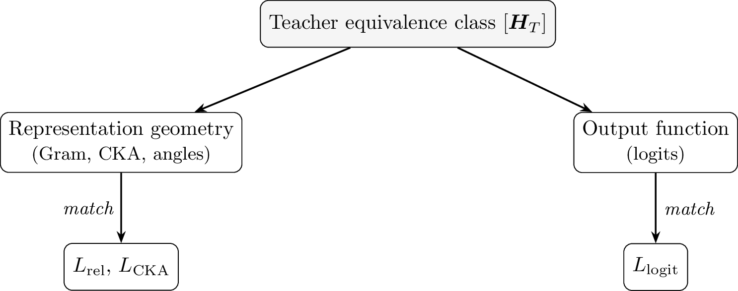
4 is the whole argument at a glance: because the teacher is a class, one does not match \(\boldsymbol{H}_T\) to the student directly; one matches what the class actually determines—its representation geometry, its output function, or both.
Having seen the three families concretely, we state the criterion that separates them.
Definition 6 (Admissible distillation objective). An objective is admissible* if it depends on the teacher only through a quotient of the class action—it factors as \(\mathcal{L}=\bar\mathcal{L}\circ\pi\) for some \(\pi\in\{\pi_{\mathrm{rep}},\pi_{\mathrm{joint}}\}\), hence is constant on the fibers \(\pi\) collapses. Its level is the coarsest such quotient: families (A) and (B) sit at the representation level (\(\pi_{\mathrm{rep}}\)), transferring representation geometry; family (C) sits at the joint level (\(\pi_{\mathrm{joint}}\)), a function of \(f_S\) alone, which is why it transfers capability. Absolute feature matching is not admissible (1): it separates points of a single fiber. Since the invariants are relative to \(\mathcal{X}\), what any objective transfers is a function of teacher \(\times\,\mathcal{X}\), bounded above by the teacher (\(\boldsymbol{H}_S\preceq\boldsymbol{H}_T\)).*
6 Predicting Graft Success from Subspace Overlap↩︎
The same equivalence–class view that organized distillation predicts when module transfer works. Grafting takes a block from one model and drops it into another; sometimes it works, sometimes it destroys the network, and prior work has largely left the difference unexplained. The class view supplies the missing variable. A grafted block is read by the host’s downstream layers, and those layers expect features in a particular subspace—the donor’s block speaks in its own basis, and the host can use it only to the extent the two share that subspace. The intuition is linguistic: two English speakers understand each other; an English and a Chinese speaker, handed the same word, do not. A layer’s output is a feature dictionary, and the next layer can read it only if the dictionaries overlap. We therefore expect graft success to be governed not by absolute features but by how much the donor and host representations share a subspace at the seam—a basis–invariant quantity, exactly the kind 3 identified.
We fix terminology. Grafting inserts a module (one or more layers) taken from a donor model into a host model in place of the host’s own, a setting studied empirically as model (or network) stitching [13], [14] and closely related to the permutation and linear–mode–connectivity symmetries of trained networks [15], [16]. We deliberately write donor and host rather than teacher and student: grafting is not knowledge transfer from one model to another (there is no \(S\preceq T\) relation and no objective being minimized) but a part transplant, in which the host keeps most of its body and swaps in one block from the donor. The two roles are asymmetric in a way teacher/student is not—the host supplies the surrounding network, the donor a single module—so the stitching vocabulary fits better.
Definition 7 (Seam). The seam* is the interface between the donor module and the host network at which the donor–side representation \(\boldsymbol{H}_D\) becomes the input read by the host’s downstream layers, whose own boundary representation is \(\boldsymbol{H}_H\). Both \(\boldsymbol{H}_D\) and \(\boldsymbol{H}_H\) are taken on a common probe set at this interface.*
A graft succeeds when it preserves the network’s function (operationally, when the grafted model’s perplexity stays close to the host’s; we use \(\mathrm{PPL}_{\text{graft}}/\mathrm{PPL}_{\text{host}}<2\) in the experiment). We posit that this success is governed by the overlap of the two feature subspaces at the seam.
Assumption 2 (Overlap governs transfer). The probability that a graft preserves function depends on \((\boldsymbol{H}_D,\boldsymbol{H}_H)\) only through equivalence–class invariants of their joint configuration, monotonically in the degree of shared subspace.
Candidate scalar invariants are \(\mathrm{CKA}(\boldsymbol{H}_D,\boldsymbol{H}_H)\), the Procrustes residual \(\rho\) of 4, and \(k_{\mathrm{eff}}\). Here donor and host carry independent bases (each is identified only up to its own \(\mathcal{G}\)–action), so the relevant invariance is the separate–argument one of 3—constant under the action applied to either argument on its own—not the joint action of 2, which couples a single representation to its own reader. All three candidates have this property.
Prediction 1 (Monotonicity). Graft success rate increases monotonically with \(\mathrm{CKA}(\boldsymbol{H}_D,\boldsymbol{H}_H)\) and decreases monotonically with the Procrustes residual \(\rho\).
Prediction 2 (Domain effect is mediated by overlap). Pairs pretrained on matched domains exhibit higher boundary CKA, and the effect of domain match on graft success is mediated by CKA: conditioning on CKA, the residual direct effect of domain match is small. The claim is causal in structure—domain match does not help grafting directly; it helps because matched domains produce more overlapping representations (\(\text{domain}\to\text{overlap}\to\text{success}\)), and it is the overlap, not the domain label, that the graft responds to. This is the mechanism behind the empirical finding that domain alignment is the decisive variable.
Prediction 3 (Alignment helps most under mismatch). Inserting a low–capacity alignment map \(\boldsymbol{W}\) (4) before the graft raises success most for low–overlap pairs and least for high–overlap pairs, i.e.there is a negative interaction between baseline overlap and the benefit of explicit alignment. High–overlap pairs are already aligned, so there is little left to correct.
6.0.0.1 Empirical protocol.
From grafting runs, collect for each donor–host pair the boundary representations \((\boldsymbol{H}_D,\boldsymbol{H}_H)\) on a fixed probe set together with a success/failure label. Then: (1) compute \(\mathrm{CKA}\), \(\rho\), \(k_{\mathrm{eff}}\); (2) regress success on each invariant to test 1; (3) run a mediation analysis \(\text{domain}\to\mathrm{CKA}\to\text{success}\) for 2; (4) ablate the alignment map \(\boldsymbol{W}\) and test the overlap\(\times\)alignment interaction for 3.
6.0.0.2 Controlled validation (Qwen2.5–0.5B).
We instantiate this protocol with a layer–transplant experiment. Donor variants are produced by perturbing chosen layers of the host to varying strengths, spreading boundary overlap across \(\mathrm{CKA}\in[0.31,1.00]\); each donor’s perturbed layer block is transplanted into a fresh copy of the host, with success as defined above (\(\mathrm{PPL}_{\text{graft}} /\mathrm{PPL}_{\text{host}}<2\)). Over \(135\) grafts (success rate \(0.64\)), boundary overlap predicts success as 1 requires: \(\mathrm{CKA}\) enters the success logit with coefficient \(+60\) (AUC \(0.79\)) and the Procrustes residual \(\rho\) with coefficient \(-9.5\) (AUC \(0.79\)); the continuous quality \(-\log(\mathrm{PPL}\text{ ratio})\) correlates \(+0.59\) with \(\mathrm{CKA}\) and \(-0.76\) with \(\rho\).
The experiment also sharpens the claim. Overlap is necessary but not sufficient: low–overlap grafts almost always fail, but high–overlap grafts near the output (e.g.transplanting layers \(20\)–\(21\) of \(24\)) fail even at \(\mathrm{CKA}\approx1.00\), because layers close to the readout amplify small mismatches into large output changes. Graft success is thus governed by boundary overlap together with transplant depth—overlap sets the ceiling, depth governs sensitivity. This is consistent with 2 as a monotone (not deterministic) relationship.
We note the scope of this evidence. The donors here are controlled perturbations of the host, so the study validates the overlap–predicts–success relationship (1) within a single model family; it does not by itself establish the cross–model mediation of 2, which would require genuinely distinct pretrained donors. We therefore present 2 as a prediction motivated by the controlled result and by the prior observation that domain alignment is decisive in practice, and leave its cross–model test to future work.
7 Experiments: Restoration and Distillation on Qwen2.5↩︎
We test the theory directly, beginning with a controlled restoration experiment. The question is sharp: if we damage a pretrained model and then re-train it using only a basis–invariant signal, does the model’s pretraining—and its capability—come back? The final result (7.9) then moves beyond restoration to genuine cross–width distillation between independently pretrained models, and finds the same ordering.
7.0.0.1 Scope.
Our central claims are theoretical—the ill–posedness of absolute matching and the identification of admissible invariant targets hold for any architecture satisfying 1. The experiments below are controlled validations on Qwen2.5 and Llama–3.1, intended to test the theory’s consequences rather than to demonstrate a production distillation system or large–scale cross–model transfer; the cross–width distillation of 7.9 is the one genuine (non–restoration) transfer we run, and it remains modest in scale. Where a claim (e.g.cross–model graft mediation) exceeds what the controlled setup tests, we say so explicitly.
7.1 Setup↩︎
All code, data, and the exact per–result mapping used below are available at https://github.com/MachineLearningHan/Invariant_Pgm; each script carries a comment naming the result it produces, and the repository’s index links every result and table in this section to the script that generates it.
The primary teacher \(T\) is Qwen2.5–0.5B [17] (24 decoder layers, tied input/output embeddings), held frozen. A student \(S\) is obtained by corrupting \(T\): we re-initialize a fraction \(s\) of the middle decoder layers (protecting the first and last two, since tied embeddings make the output head sensitive to embedding damage). Stage 1 trains \(S\) to match \(T\) with a basis–invariant per–layer objective; no label supervision and no teacher logits are used in the pure basis–invariant runs. We compare three objectives: \(L_{\mathrm{cka}}\) and \(L_{\mathrm{rel}}\) (basis–invariant, 5), and \(L_{\mathrm{abs}}\) (the ill–posed coordinate–matching control of 1). All Stage 1 training matches last–token pooled representations across all layers on a generic text corpus.
To probe scale and, crucially, the role of weight tying, we repeat the experiment on two untied models from different families: Qwen2.5–7B–Instruct [17] (28 decoder layers, hidden width \(3584\)) and Llama–3.1–8B–Instruct [18] (32 decoder layers, hidden width \(4096\)), both of which untie the input embedding from the output head. For these runs we train only the corrupted layers (and, where noted, the output head) to keep the optimizer state tractable; this restriction makes the tying distinction observable, as shown below. Using two distinct families lets us check that the tying effect is not an artifact of a single architecture.
7.1.0.1 What this design is, and is not.
A word on scope, since the setup governs how the numbers below should be read. The student is not an independent model: it is the teacher with a fraction of its layers re–initialized, so it shares the teacher’s architecture, width, tokenizer, and—crucially—the uncorrupted layers verbatim. Those surviving layers keep the student near the teacher’s own representative of the class: the two start in a largely shared coordinate frame, not in the independent frames that two separately pretrained models would occupy. This is deliberate. The experiment is a controlled probe of the theory’s mechanism—it isolates what drives capability (the output function, 3) from what merely aligns geometry (a representational invariant)—by holding the coordinate system fixed so that the two objectives can be compared on equal footing. It is therefore a damage–and–restore study, not a cross–model distillation benchmark. The harder case, where teacher and student are independently trained and occupy different representatives (or differ in width, 3), is exactly where the alignment of 4 becomes necessary rather than incidental; our controlled setup does not test it, and we do not claim it (1). What the study does establish—cleanly, because the frame is shared—is that even with the representation held recoverable, capability returns only through the output–function term, which is the proposition it was built to test.
We measure restoration at two levels. Representational: per–layer \(\mathrm{CKA}(S,T)\) on held–out probes, judged against a permutation null. Functional (capability): \(\mathrm{KL}(T\Vert S)\) over next–token distributions, perplexity ratio \(\mathrm{PPL}_S/\mathrm{PPL}_T\), and top–1 next–token agreement. Probes are split into an in–domain set (the language/domain of the training corpus) and an out–domain set (a disjoint domain), to test whether restoration is confined to the subspace the corpus spans.
7.2 Result 1: Basis–invariant training restores representation, not capability↩︎
With \(L_{\mathrm{cka}}\) alone, per–layer \(\mathrm{CKA}(S,T)\) recovers from the corrupted baseline (\(\approx 0.90\)) to \(0.99\)–\(1.00\) in–domain across all corruption strengths—the representational geometry is restored from a label–free, basis–invariant signal. Yet the function is not: 4 (left block) shows \(\mathrm{KL}(T\Vert S)\approx 7\) – \(11\), perplexity ratios of \(10^2\) – \(10^4\), and near–zero top–1 agreement. A model can have \(\mathrm{CKA}=0.99\) and still be a different function. This is the empirical face of the equivalence–class structure: \(L_{\mathrm{cka}}\) drives \(S\) close to \([H_T]\) on the probe set (high \(\mathrm{CKA}\)) but does not select the representative the (tied) output head reads, so the logits—and the capability—remain wrong.
7.3 Result 2: Capability is driven by the logit term, not by representational matching↩︎
Adding a full–sequence logit–distillation term \(\mathcal{L}=\lambda_{\ell}L_{\mathrm{logit}}+\lambda_r L_{\mathrm{cka}}\) recovers capability: in–domain perplexity ratio \(1.01\times\), top–1 \(0.98\); out–domain \(1.06\times\), \(0.72\) (4, right). The logit term must be applied over the full sequence—matching only the last token drives the last–token KL to \(0.03\) during training yet leaves the full–sequence KL at \(\approx 6\) and perplexity \(>700\times\).
An ablation isolates the source of the recovery, and the result is sharper than “both terms help.” On the hardest setting—every decoder layer re–initialized (Result 6) with the corpus widened so coverage is not the bottleneck—we compare \(L_{\mathrm{cka}}\) alone, \(L_{\mathrm{logit}}\) alone, and the sum (3). Representational matching alone drives \(\mathrm{CKA}\) to \(0.999\) but leaves capability destroyed (perplexity ratio \(\sim\!10^6\), top–1 \(0\)). The logit term alone—which never references the hidden representation—recovers capability essentially perfectly (ratio \(1.0\times\), top–1 \(1.00\)) while leaving \(\mathrm{CKA}\) at only \(0.89\). The two are near–orthogonal: \(L_{\mathrm{cka}}\) aligns representational geometry, \(L_{\mathrm{logit}}\) restores the function, and the function does not follow from the geometry. This is the training–level form of the rotation result of 1: there, a function–preserving reparametrization moved the feature–matching loss while leaving the invariants fixed; here, optimizing the invariant (\(L_{\mathrm{cka}}\)) moves the representation into place while leaving the function fixed—wrong, in the same way and for the same reason.
We read this as the central empirical lesson rather than a negative result. It is the experimental face of the theory: capability is a property of the output function, which is an invariant of the equivalence class, and \(L_{\mathrm{logit}}\) targets exactly that invariant (5). A representational objective such as \(L_{\mathrm{cka}}\) drives \(S\) close to \([H_T]\) on the probe set (high \(\mathrm{CKA}\)) but is free to pick any representative, so it need not—and here does not—preserve the function. The right prescription is therefore not “match representations with a basis–invariant loss” but “match the output–function invariant (\(L_{\mathrm{logit}}\)); use a representational invariant only when the geometry itself is the goal.” The combined objective (\(L_{\mathrm{cka}}+ L_{\mathrm{logit}}\)) restores both geometry and function (4 3) but the capability comes from the logit term.
| objective | \(\CKA\) | PPL ratio | \(\mathrm{KL}(T\!\parallel\!S)\) | top–1 |
|---|---|---|---|---|
| \(L_{\mathrm{cka}}\) only | 0.999 | \(\sim\!3\times10^6\) | \(\gg\!1\) (diverged) | \(\approx\!0.00\) |
| \(L_{\mathrm{logit}}\) only | 0.894 | \(1.02\times\) | \(\approx\!0.05\) | \(0.99\) |
| \(L_{\mathrm{cka}}+L_{\mathrm{logit}}\) | 0.992 | \(1.07\times\) | small | \(0.92\) |
| \(L_{\mathrm{cka}}\) only | \(+\,L_{\mathrm{logit}}\) (full–seq) | ||||||||
|---|---|---|---|---|---|---|---|---|---|
| 2-5(lr)7-10 Probe | \(\CKA\) | KL | PPL ratio | top–1 | \(\CKA\) | KL | PPL ratio | top–1 | |
| in–domain | 0.998 | 7.56 | \(742\times\) | 0.02 | 0.99 | 0.019 | \(1.01\times\) | 0.98 | |
| out–domain | 0.533 | 5.31 | \(315\times\) | 0.02 | 0.99 | 0.045 | \(1.06\times\) | 0.72 | |
7.4 Result 3: Restoration is confined to the corpus–covered region↩︎
In–domain probes restore far more than out–domain ones at every level. Throughout, “region” (and, loosely, “subspace”) refers to the part of representation space that the training corpus and probes actually cover—an empirical, distributional notion (training/probe coverage), not a linear subspace we measure and project onto. With \(L_{\mathrm{cka}}\) only, out–domain \(\mathrm{CKA}\) can collapse (e.g.\(0.53\) at \(s=0.4\), mean over four seeds \(0.61\pm0.07\)) while in–domain stays at \(0.99\), a representational gap of up to \(+0.47\). The capability gap persists even after the logit term: in–domain top–1 \(0.98\) versus out–domain \(0.72\). The mechanism is the training subspace: when out–domain text is added to the corpus, the out–domain gap vanishes—\(\mathrm{CKA}\) rises \(0.53\to0.996\) and the gap drops to \(+0.001\), with out–domain capability following (PPL ratio \(1.06\times\)). Restoration is therefore governed not by corruption strength but by whether the corpus spans the relevant subspace: the model is restored to the teacher on, and only on, the subspace the training data covers. The non–monotonicity in corruption strength (the worst out–domain \(\mathrm{CKA}\) occurs at intermediate \(s\)) is explained the same way: at that strength the corruption happens to destroy out–domain–bearing layers that the in–domain corpus cannot repair; it is not a property of the damage but of the damage–corpus alignment.
This is the empirical face of the probe–set dependence noted in 2: the invariants, and hence what a basis–invariant objective can constrain, are defined relative to the probes the objective actually sees. Training on a corpus is choosing the probe set \(\mathcal{X}\) over which \(\boldsymbol{H}(\mathcal{X})\) is matched; coverage is restored exactly on \(\mathrm{span}\,\boldsymbol{H}(\mathcal{X})\) and not beyond it. “Teacher \(\times\) corpus” is, in this notation, teacher \(\times\, \mathcal{X}\).
7.5 Result 4: The coordinate–matching control degrades under coordinate destruction↩︎
1 predicts \(L_{\mathrm{abs}}\) is ill–posed when the student may sit at a different representative of \([H]\). When corruption is mild the surviving layers keep \(S\) in \(T\)’s coordinate frame, and \(L_{\mathrm{abs}}\) performs comparably to \(L_{\mathrm{cka}}\). As corruption destroys more of that frame the gap appears: at \(s=1.0\), \(L_{\mathrm{cka}}\) reaches in/out \(\mathrm{CKA}= 0.994/0.897\) versus \(L_{\mathrm{abs}}\) at \(0.967/0.850\). The control is not catastrophic here because re–initialization preserves coordinates more than a free orthogonal reparametrization would; the predicted advantage of the basis–invariant objective grows precisely as the shared coordinate frame is removed, consistent with 1.
7.6 Result 5: Scale, and the role of weight tying↩︎
The same pattern holds at \(7\)B, with one mechanistically informative difference driven by weight tying. On Qwen2.5–7B–Instruct (untied head), basis–invariant training again restores representation (in–domain \(\mathrm{CKA}\approx0.97\)) without restoring capability. Adding the full–sequence logit term while training only the corrupted layers leaves the head frozen, and in–domain capability only partially returns (PPL ratio \(2.3\times\)). Once the output head is added to the trainable set, in–domain capability is recovered (PPL ratio \(1.2\times\), top–1 \(0.94\)); out–domain follows only when out–domain text is mixed into the corpus (PPL ratio \(1.4\times\), top–1 \(0.82\)), reproducing the subspace–confinement of Result 3 at scale. The same behavior reproduces on Llama–3.1–8B–Instruct, a different untied family: in–domain capability is recovered with the head trainable (PPL ratio \(1.00\times\)), and out–domain follows under corpus mixing (PPL ratio \(1.10\times\), top–1 \(0.92\)). 5 summarizes all three models.
The tying distinction is the point. In the tied 0.5B model the output head is the input embedding, which we never corrupt, so fixing the output coordinate frame happens automatically and the logit term suffices. In the untied models the head is a separate parameter: a basis–invariant objective drives the hidden representation close to \([H_T]\) on the probe set, but the specific representative the (independent) head reads must be selected by training the head itself. That the same head–training requirement appears in two unrelated untied families (Qwen and Llama) indicates it is a property of untying, not of a particular architecture. This is the same single mechanism—fixing the output coordinate frame—in two guises: implicit via shared weights when tied, explicit via head training when untied. The head–ablation contrast (PPL \(2.3\times\) head–frozen vs \(1.2\times\) head–trained, in–domain) isolates it.
One might object that this reduces the geometric story to a mundane fact—“of course one must tune the output head to a new representation.” The objection misreads what is being explained. A bare appeal to head–tuning predicts nothing about when it is needed; the equivalence–class account does. It says the output head fixes a representative within \([H_T]\), so tuning is required exactly when that representative is not already pinned—i.e.in the untied case, where the head is an independent parameter—and is not required when weight tying pins it automatically, as in the 0.5B model where \(L_{\mathrm{logit}}\) alone suffices with the head frozen. The tied/untied split, and the fact that the identical requirement recurs across two unrelated untied families, is the content: it is the joint action of 1 (representation and its reader move together) observed at the readout, not a restatement of “train the head.” Capability being the output–function invariant is what makes the head the only thing that still needs selecting once the representation is in the right class.
| in–domain | out–domain | ||||
|---|---|---|---|---|---|
| 3-4(lr)5-6 Model | objective | PPL ratio | top–1 | PPL ratio | top–1 |
| 0.5B (tied) | \(L_{\mathrm{cka}}\) | \(742\times\) | 0.02 | \(315\times\) | 0.02 |
| 0.5B (tied) | \(+L_{\mathrm{logit}}\) | \(1.01\times\) | 0.98 | — | — |
| 0.5B (tied) | \(+L_{\mathrm{logit}}\), \(+\)mix | — | — | \(1.06\times\) | 0.72 |
| 7B (untied) | \(+L_{\mathrm{logit}}\), head frozen | \(2.3\times\) | 0.87 | \(88\times\) | 0.08 |
| 7B (untied) | \(+L_{\mathrm{logit}}\), \(+\)head | \(1.2\times\) | 0.94 | \(211\times\) | 0.07 |
| 7B (untied) | \(+L_{\mathrm{logit}}\), \(+\)head, \(+\)mix | \(1.3\times\) | 0.94 | \(1.4\times\) | 0.82 |
| 8B–Llama (untied) | \(+L_{\mathrm{logit}}\), \(+\)head | \(1.00\times\) | 0.80 | \(159\times\) | 0.12 |
| 8B–Llama (untied) | \(+L_{\mathrm{logit}}\), \(+\)head, \(+\)mix | \(0.98\times\) | 0.87 | \(1.10\times\) | 0.92 |
7.7 Result 6: Decoder–from–scratch reconstruction, and what does the work↩︎
The strongest version of the setup discards the pretrained decoder entirely. Where Result 2 used the all–layers–reinitialized setting to decompose the objective (which term recovers capability), here we hold the objective fixed and ask a different question—how far reconstruction reaches as a function of corpus coverage. We re–initialize all decoder layers, keeping only the embedding/unembedding—i.e.the input/output coordinate system, which is fixed by the tokenizer and which we treat as given rather than as a pretrained capability. We then ask whether distillation can rebuild the decoder from the teacher alone. With the combined objective and a corpus that covers both probe domains, it can: in– and out–domain perplexity ratios both reach \(\approx 1.0\times\) (top–1 \(0.92\) and \(0.84\)) starting from fully random decoder layers. Coverage is the binding constraint, exactly as in Result 3: with an in–domain–only corpus the out–domain perplexity ratio is \(\sim\!10^4\), and adding out–domain text to the corpus collapses it to \(1.0\times\). So the corpus, not the pretrained weights, determines which subspace is reconstructed—the reconstruction is a function of teacher \(\times\,\mathcal{X}\) (the probe set the corpus induces).
The ablation of Result 2 was run in exactly this all–layers setting, and it tells us what does the work: the reconstruction is driven by \(L_{\mathrm{logit}}\), not by the representational objective. This bounds the practical reading of “decoder–from–scratch.” What is being transferred is the teacher’s output function, on the subspace the corpus illuminates, via output–function matching; the basis–invariant analysis explains why that transfer is well–posed (the output is a class invariant) but the representational loss is not the mechanism. We keep the embedding/unembedding precisely because it is the shared coordinate system the output–function invariant is expressed in; reconstructing it as well is left to future work. Pretraining retains its value where this picture does not reach: creating the first teacher, and covering subspaces no distillation corpus does.
7.8 Result 7: Cross–width restoration, and a teacher–forced/generation gap↩︎
The controlled studies above hold width fixed. This result and the next (7.9) are preliminary cross–width probes—single model pairs, a WikiText probe set, and short training—not scaled distillation claims; we report them for the direction they establish, not as production numbers. A preliminary probe at unequal width—the case 3 addresses—sharpens the picture and exposes a limit the teacher–forced metrics hide. Here the teacher is Qwen2.5–1.5B (\(d_T=1536\), \(28\) layers) and the student Qwen2.5–0.5B (\(d_S=896\), \(24\) layers), sharing the tokenizer and vocabulary (\(V=151{,}936\)); the student is corrupted by re–initializing its middle layers and restored on a WikiText probe set. We compare (ii) logit only (\(L_{\mathrm{logit}}\), 10 ) and (iii) ridge–Procrustes alignment followed by logit (“\(\boldsymbol{W}\) first, then logit,” 3), across seeds, and add generation–side metrics: the repetition rate and distinct–\(n\) of the student’s own free–running greedy generation, and the rollout KL—\(\mathrm{KL}(T\Vert S)\) averaged along the teacher’s greedy rollout, a soft trajectory match that, unlike top–1, does not penalize a different–but–reasonable next token.
Three findings, stated with their scope. First, logit–KD transfers capability across unequal width with no alignment: top–1 agreement reaches \(\approx0.98\) from a corrupted start, using only \(L_{\mathrm{logit}}\) on the shared vocabulary—no \(\boldsymbol{W}\), no common hidden frame, consistent with 3 and the ordering discussion of 5. Second, adding the alignment map \(\boldsymbol{W}\) buys nothing measurable, and at an effective weight tends to hurt: when the feature term is weak enough not to dominate, (iii) matches (ii) on top–1, on generation repetition, and on rollout KL (the last essentially identical, \(\approx1.25\) nats for both), while costing roughly twice the wall–clock; when the feature term carries a non–trivial weight it does not merely add nothing but destabilizes the otherwise smooth logit–only convergence—across seeds the \(\boldsymbol{W}\)–plus–logit run oscillates and, on some seeds, diverges, whereas logit alone converges cleanly to top–1 \(\approx1.0\). Either way the feature term never improves on logit alone. This is the cross–width form of the ablation (7.3) and matches the mild harm seen in 6: capability rides on the output function, so a feature alignment that does not change the output does not change capability—and, in this restoration setting, does not improve generation either. Third, and least expected, teacher–forced capability outruns free–running generation: at top–1 \(\approx0.98\) the rollout KL is still \(\approx1.25\) nats and the student’s greedy generations, though locally fluent (grammatical, on–topic WikiText prose), drift from the teacher’s trajectory and are prone to repetition loops and invented specifics. The one–step output–function match that 3 guarantees does not by itself guarantee trajectory stability under autoregression.
We report this as a preliminary result: a single model pair, one corruption recipe, a small probe set, and few seeds—enough to establish the direction (logit suffices, \(\boldsymbol{W}\) does not help, a teacher–forced/generation gap exists) but not to quantify the gap across scales or architectures. It refines rather than overturns the theory: capability, defined as the one–step output function, transfers as 3 predicts; the gap is a reminder that generation quality is a property of the whole trajectory, which a per–token invariant constrains only indirectly. Stated precisely, and used consistently below: one–step output–functional capability is restored, but autoregressive trajectory capability is not guaranteed—“capability restored” in this paper always means the former. Closing the gap—whether by training the corrupted layers beyond the seam, or by a trajectory–level objective—is left to future work.
7.9 Result 8: Feature–only collapse in a genuine cross–width distillation setting↩︎
The previous results established the theory under controlled restoration, where the student is a corrupted copy of the teacher. We now ask whether the same conclusion survives genuine cross–width distillation between independently pretrained models—the setting practitioners actually mean by “distillation.” Result 7 held out the third leg of the ablation. It compared (ii) \(L_{\mathrm{logit}}\) and (iii) \(\boldsymbol{W}\)–then–\(L_{\mathrm{logit}}\), but not the feature term alone. The feature term here is \(L_{\mathrm{fm}}\), the coordinate–matching family of \(L_{\mathrm{abs}}\) (1) rather than the relational \(L_{\mathrm{cka}}\) of 3; both are feature–matching objectives, and the point of interest is that either one, taken alone, collapses the model—so this supplies the cross–width, coordinate–matching counterpart of the \(L_{\mathrm{cka}}\)–only row of 3. Result 7 was also a restoration study: the student was a corrupted copy of the teacher. Here we close both gaps. The student is a pristine pretrained Qwen2.5–0.5B (no corruption), the teacher is Qwen2.5–1.5B, and we run genuine unequal–width distillation on a WikiText–103 corpus with the shared vocabulary (\(V=151{,}936\)). The feature term \(L_{\mathrm{fm}}\) pulls the student’s anchor–layer hidden states onto the teacher’s through a learned projection (\(896\!\to\!1536\), per anchor), the unequal–width instance of the map \(\boldsymbol{W}\) of 3. Concretely, for a set of anchor layer pairs \(\mathcal{A}=\{(\ell,\ell')\}\) matching student layer \(\ell\) to teacher layer \(\ell'\), and a per–anchor linear map \(\boldsymbol{W}_\ell:\mathbb{R}^{d_S}\!\to\!\mathbb{R}^{d_T}\), \[\label{eq:lfm} L_{\mathrm{fm}} =\frac{1}{|\mathcal{A}|}\sum_{(\ell,\ell')\in\mathcal{A}} \big\lVert\, \boldsymbol{H}^{(\ell')}_T \;-\; \boldsymbol{W}_\ell\,\boldsymbol{H}^{(\ell)}_S \,\big\rVert_F^2 ,\tag{12}\] averaged over probe tokens. This is the unequal–width, \(\boldsymbol{W}\)–mediated form of the coordinate–matching loss \(L_{\mathrm{abs}}\) of 1: with \(d_S=d_T\) and \(\boldsymbol{W}_\ell=I\) it reduces to \(L_{\mathrm{abs}}\), and like \(L_{\mathrm{abs}}\) it is not constant on the student’s equivalence class, so 1 applies. In the full model \(\boldsymbol{W}_\ell\) is learned jointly; in the surrogate below it is instead the closed–form ridge optimum recomputed each step, giving the feature term its best case. Crucially we drop the cross–entropy ground–truth term entirely, so each objective is measured in isolation on the soft teacher signal.1
| objective | WikiText–103 val PPL | vs base |
|---|---|---|
| base (untrained student) | \(21.15\) | — |
| (i) \(L_{\mathrm{fm}}\) only | \(>10^{6}\) (all seeds) | collapse |
| (ii) \(L_{\mathrm{logit}}\) only | \(\mathbf{20.77\pm0.03}\) | \(-1.77\%\) |
| (iii) \(L_{\mathrm{fm}}+L_{\mathrm{logit}}\) | \(20.94\pm0.02\) | \(-1.01\%\) |
7.9.0.1 Three–way result.
6 reproduces the same–architecture ablation of 3 in the genuine cross–width, from–pristine setting, and the three rows are the three legs of the theory. (i) The feature term alone drives perplexity above \(10^{6}\) on every seed (from \(1.6\times10^{6}\) to \(3.3\times10^{8}\)): matching hidden coordinates through \(\boldsymbol{W}\), with no term that references the output, does not merely fail to help—it destroys a model that started out working. The mechanism is the one 1 names: \(L_{\mathrm{fm}}\) moves the student to some representative of \([H_T]\) while the unembedding, which receives no gradient, still expects the old representative, so the output function is broken. (ii) The logit term alone—which never touches the hidden state—keeps the student slightly below its original perplexity (\(20.77\pm0.03\) vs.\(21.15\)), exactly as 3 predicts: capability is the output–function invariant, and \(L_{\mathrm{logit}}\) targets it directly, across a width change and with no alignment map. (iii) Adding \(L_{\mathrm{fm}}\) on top does not help and in fact hurts by a small but consistent and significant margin: paired across the three seeds, \(L_{\mathrm{fm}}+L_{\mathrm{logit}}\) is worse than \(L_{\mathrm{logit}}\) by \(+0.160\pm0.009\) PPL, the same sign in every seed (\(\text{diff}/\text{pooled std}\approx7\)). This is the cross–width form of “\(\boldsymbol{W}\) buys nothing” (7.8), sharpened: a feature alignment that the logit term does not already imply is not neutral but a mild distraction from the objective that actually carries capability. The surrogate below shows that when \(\boldsymbol{W}\) is instead solved to optimality the harm vanishes into noise—so the honest statement across both settings is that the feature term ranges from neutral (optimal \(\boldsymbol{W}\)) to mildly harmful (learned \(\boldsymbol{W}\)), and is never beneficial.
7.9.0.2 A controlled cross–check with a learned–optimal alignment.
A referee could object that \(L_{\mathrm{fm}}\) fails only because the projection is under–trained. We rule this out with a small controlled surrogate in which the alignment is solved to optimality at every step. Teacher and student are tiny transformers of different width (\(d_T=64\), \(L_T=4\) vs.\(d_S=32\), \(L_S=3\)) trained on a synthetic noisy–bigram language; the feature map \(\boldsymbol{W}\) is the closed–form ridge solution recomputed each step, so the feature objective is given its best case. All metrics are computed on a held–out probe set the student never trains on, over five seeds. We report top–1 agreement with the teacher, free–running greedy generation agreement, and the student’s own held–out perplexity (7).
| objective | top–1 (vs T) | gen (vs T) | self–PPL |
|---|---|---|---|
| (i) \(L_{\mathrm{fm}}\) only | \(0.031\pm0.005\) | \(0.017\pm0.014\) | \(\sim\!9\times10^{5}\) |
| (ii) \(L_{\mathrm{logit}}\) only | \(0.208\pm0.017\) | \(0.200\pm0.047\) | \(1281\pm731\) |
| (iii) \(\WW+L_{\mathrm{logit}}\) | \(0.227\pm0.019\) | \(0.175\pm0.040\) | \(1428\pm379\) |
The surrogate confirms two of the three legs sharply and refines the third. On function agreement the picture matches the full model: the logit term raises top–1 and generation agreement roughly four–fold over the feature term (leg i, leg ii), and adding the optimal \(\boldsymbol{W}\) changes top–1 by \(-0.001\) and generation by \(-0.004\), within the pooled seed noise (leg iii). With \(\boldsymbol{W}\) at optimality the feature term is thus neutral, whereas with the learned \(\boldsymbol{W}\) of the full model (6) it is mildly harmful; in neither regime does it help. “\(\boldsymbol{W}\) buys nothing” holds in the strong form—it holds even when \(\boldsymbol{W}\) is solved to optimality, not merely learned. This does not refute objective family (B) (5): when a downstream consumer explicitly needs features in a shared frame—grafting, activation transplants, intermediate–layer hints—aligned features are the point, and \(L_{\mathrm{fm}}\) is the right tool for that job. What 6 shows is narrower and compatible with it: feature matching alone is not a capability objective. As a supervision signal for transferring what the teacher can do, it does not substitute for the output–function term, and adding it on top of that term does not help. Across all three metrics the surrogate agrees with the real model: under \(L_{\mathrm{fm}}\) alone, top–1 and generation sit at chance and the student’s own held–out perplexity blows up to \(\sim\!10^{5}\) (7, row i). Feature–only matching does not leave a self–fluent–but–disconnected student; it simply fails to build a working model, exactly as in the full run (6).
7.9.0.3 Scope.
6 is three seeds on one model pair; 7 is five seeds on a synthetic different–width pair. Together they establish the direction—feature–only collapses, logit suffices, \(\boldsymbol{W}\) ranges from neutral to mildly harmful and never helps—with the feature–only leg now supplied in both the genuine and the controlled setting. Both remain modest in scale: one real corpus and one synthetic language, a single width ratio each, and \(\le\!2000\) training steps. We therefore report the collapse as a robust empirical fact in this cross–width distillation setting, not as a proof that feature–only matching must fail in every regime; the theory (1) explains why it fails when it does, but a differently–wired objective that also selects the reader’s representative could behave differently. Quantifying the collapse across scales, width ratios, and untied–head architectures is left to future work, alongside the trajectory–level gap of 7.8. To restate the scope of the negative result precisely: it concerns feature matching used as a capability objective, and does not deny feature alignment where it is genuinely needed—grafting, activation transplants, and other coordinate–consuming modules, where a downstream reader requires a specific frame and \(\boldsymbol{W}\) is therefore conditionally valuable, exactly as 5 sets out. The claim here is only that such alignment is not, by itself, a route to transferring capability.
7.10 Takeaways↩︎
The experiments separate two things the phrase “restore the model” conflates. A basis–invariant objective restores the representation’s equivalence–class structure cheaply and label–free, but representation is not function: a logit term over the full sequence is required to fix the output coordinate frame and recover capability. And restoration—both representational and functional—is confined to the subspace spanned by the training corpus, exactly the “restored near the fine–tuning subspace” statement, made quantitative. The scale experiment adds a third clause: fixing the output coordinate frame is implicit under weight tying but must be done explicitly—by training the head—when the head is untied, as it is in most large models.
The sharpest lesson is from the ablation. Aligning representations with a basis–invariant loss and recovering the teacher’s function are near–orthogonal: \(L_{\mathrm{cka}}\) alone reaches \(\mathrm{CKA}\approx1\) with capability destroyed, \(L_{\mathrm{logit}}\) alone recovers capability with \(\mathrm{CKA}\) left low. The practical driver of capability transfer is output–function matching; the contribution of the basis–invariant framework is not a better representational loss but the explanation—the output function is the class invariant, which is why logit distillation is well–posed and why matching hidden coordinates directly is not. This is a more useful claim than “use a basis–invariant objective,” and the data support it directly. The same ordering survives outside the controlled restoration setting: in genuine unequal–width distillation from a pristine student (7.9), the feature term alone collapses the model, the logit term alone slightly improves it, and adding the feature term does not help—so the lesson is not an artifact of the corruption–and–restore design.
8 Discussion↩︎
8.0.0.1 What the framework does and does not claim.
The contribution is a way to see teacher supervision, validated where its consequences are testable. The theory and the experiments meet at one point in particular: the ablation of Result 2 (7.3) is the experimental counterpart of 3. What the proposition asserts about where capability lives, the ablation confirms about what recovers it—the output–function term \(L_{\mathrm{logit}}\) restores capability while the representational term \(L_{\mathrm{CKA}}\) does not, even as it drives \(\mathrm{CKA}\to1\). Three boundaries are then worth stating plainly. First, capability transfer is driven by output–function matching; the basis–invariant analysis explains why that works (the output is the class invariant) but a representational loss is not, on its own, a capability objective (3). Second, reconstruction is bounded by corpus coverage: “teacher \(\times\,\mathcal{X}\)” is the unit of what transfers, and what the corpus does not illuminate is not recovered. Third, the controlled studies fix architecture and share the tokenizer’s embedding; cross–model and small–from–large transfer are consequences we expect but do not establish here. Fourth, and most importantly for positioning, what we study is replication, not creation. Distillation copies the teacher’s output function—on the quotient, within the corpus subspace, and bounded above by the teacher (\(S\!\preceq\!T\)); it does not produce capability the teacher lacks. The places where capability is originated rather than transferred—pretraining a first teacher, covering subspaces no corpus reaches, and pushing past the current frontier—lie outside this account by construction. This paper is about how an existing function moves through the equivalence class, not about how it first comes to exist.
8.0.0.2 Four objections, and what the evidence says.
The design invites several objections; we take the strongest head–on. (1) The restoration setup shares a coordinate frame, so of course feature matching “works” geometrically while missing the function—isn’t the collapse just damaged weights failing to return to their original coordinates? This is exactly the point, not a confound: when teacher and student already share a frame, absolute matching should be easy, yet \(L_{\mathrm{CKA}}\) still fails to restore the function while driving \(\mathrm{CKA}\!\to\!1\) (3). A confound would predict the opposite—shared frames helping feature matching. That it does not is the cleanest possible demonstration that geometry and function are distinct. And Result 8 removes the shared frame entirely: an independently pretrained, pristine student of different width shows the same collapse (7.9), so the conclusion does not rest on the restoration design. (2) Dropping cross–entropy is an extreme choice; the \(L_{\mathrm{fm}}\) collapse may reflect untuned learning rate or loss weights rather than anything about feature matching. The CE–free setup is a control, not a recommendation: we remove CE precisely so that any capability in the student comes from the distillation channel under test and not from the labels, isolating what each loss transfers. The logit channel restores the model in the very same CE–free regime (6, row ii), so the setup is not stacked against distillation as such—only against feature matching as the sole channel. (3) The collapse is an optimization failure of the alignment map \(\boldsymbol{W}\), not a representational impossibility—after all, the surrogate with an optimal \(\boldsymbol{W}\) is stable. The surrogate says the opposite. There the alignment is the closed–form ridge optimum, recomputed every step: \(\boldsymbol{W}\) is never learned and cannot be mis–optimized, yet feature–only supervision still collapses on all three metrics (top–1, generation, and self–PPL \(\sim\!10^{5}\); 7, row i). Optimal alignment removes the optimization question and the collapse remains, which is the direct evidence that the failure is structural (1), not a landscape artifact. (4) This attacks a strawman: no modern feature–based method matches absolute coordinates (\(L_{\mathrm{abs}}\)); they all insert a projection or match relationally, i.e.family (B) or (A). We agree \(L_{\mathrm{abs}}\) is a strawman, and say so—which is why the experiments use the basis–invariant \(L_{\mathrm{CKA}}\) (family A) and a learned/optimal projection \(\boldsymbol{W}\) (family B), the objectives real methods actually use, not \(L_{\mathrm{abs}}\). The finding is about those: even a relational or optimally–aligned feature objective sits on the representation quotient, so on its own it does not select the reader’s representative and does not transfer capability. \(L_{\mathrm{abs}}\) appears only as the ill–posed limit that motivates why alignment is needed in the first place; the empirical claims are all against the aligned/relational families.
8.0.0.3 The operational goal: a black–box teacher suffices, but a student model does not.
The practical content of 6 is that the student does not seek the teacher’s parameters \(\boldsymbol{W}_T\)—copying those would be a file copy, not distillation—but constructs different parameters \((\boldsymbol{H}_S,\boldsymbol{W}_S)\) landing in the same joint class, hence computing \(f_S=f_T\). This is why logit matching is the canonical objective: in the hardest honest setting, \(\boldsymbol{W}_T\) is unavailable (an API teacher, or a multi–agent system with no single \(\boldsymbol{W}_T\)), and the output is the only observable that selects the fiber—two settings share an output distribution iff they lie in the same fiber of \(\pi_{\mathrm{joint}}\) (3). It alone transfers capability (7.3) and can rebuild a decoder from random initialization (7.7). But this identifiability claim does not dispense with the student model. The logit signal is only a pointwise sample \((x,f_T(x))_{x\in\mathcal{X}}\); recovering \(f_T\) off the probe set requires generalization, and what fills the gaps is the student’s inductive bias. Were \(f_T\) linear a few points would fix it, but a transformer’s nonlinear function is not pinned down pointwise. So “inputs and outputs suffice” holds provided the student shares the teacher’s function family—which is why within–family restoration succeeds cleanly and the cross–family case is doubly hard (7.8): a mismatched tokenizer closes the output channel and a mismatched family removes the inductive bias. In short, 3 settles which function capability rides on; recovering it from finite data is a separate, estimation–level fact resting on the student’s function class.
8.0.0.4 Where cross–model transfer sits.
Because the third boundary above is the one a reader is most likely to probe, we state the paper’s position on it in one place. Our theory makes a definite prediction about independently trained models: two such models occupy different representatives of the class (12), so transferring a component between them is well–posed only after an explicit alignment onto a shared frame (5), and its success should track the overlap of the boundary subspaces being joined (2). We validate this prediction only partially, and are explicit about which part. The within–family graft study (6) confirms the overlap–predicts–success half (1) but uses controlled perturbations of one host, so it does not exercise genuinely distinct pretrained donors. The cross–width study (7.8)—Qwen2.5–1.5B into 0.5B, unequal hidden width, shared tokenizer—goes one step further: it shows the output–function mechanism (3) transfers capability across a real width gap with no shared hidden frame, and that adding the alignment map buys nothing once the logit signal is present. What remains untested is the hardest case: cross–family transfer between models with independent tokenizers and no shared vocabulary, where even the output space must be mediated. We do not run that experiment and do not claim it; it is the natural next test of 2, and the theory’s stance on it—alignment first, then an output–level objective—is a falsifiable prediction, not a demonstrated result.
8.0.0.5 Scope of the symmetry group, and a note on model merging.
Three questions about scope recur, and it is cleaner to answer them together. (i) Why \(\mathrm{O}(d)\times\mathbb{R}_+\) and not more? The absorbable group is larger: any invertible \(\boldsymbol{A}\) with \(\boldsymbol{W}_{\mathrm{in}}\mapsto\boldsymbol{A}^{-1}\boldsymbol{W}_{\mathrm{in}}\) preserves the function (13), so the full symmetry is \(GL(d)\times\)(bias shifts). We work with \(\mathrm{O}(d)\times\mathbb{R}_+\) not because the rest is absent but because our invariants (Gram, CKA) are exactly the \(\mathrm{O}(d)\times\mathbb{R}_+\)–invariants: they are blind to rotation and isotropic scale but see a general linear map, since \(\boldsymbol{H}\boldsymbol{A}\) changes \(\boldsymbol{H}\boldsymbol{H}^\top\). Matching the residual \(GL(d)\) part is precisely what the alignment of 4 estimates; the two together cover the full group. So “why only \(\mathrm{O}(d)\)” is answered by division of labor: the relational invariants handle the orthogonal part for free, alignment handles the rest. (ii) Non–orthogonal / permutation symmetry. Neuron permutations and sign flips are the discrete subgroup of \(\mathrm{O}(d)\) that also commutes with a diagonal RMSNorm gain (10), so they are covered exactly, not approximately—which is why our account connects to the permutation and linear–mode–connectivity literature [15], [16]. (iii) Model merging. Merging two independently trained models is, in these terms, an attempt to average two points that lie in different representatives of different classes; it succeeds only after the representatives are brought into a common frame, which is why permutation–alignment before averaging [16] helps for exactly the reason 4 predicts. Our framework does not claim to solve merging, but it locates the difficulty precisely: without alignment, the average of two representatives need not lie in either class, so the merged function is not controlled by either teacher. This is the same coordinate sensitivity that governs grafting (6); merging is grafting’s symmetric, two–sided case.
8.0.0.6 A direction the theory suggests: reusing capability by alignment, not retraining.
The same geometry points to a way of amortizing the cost of building capable models, which we flag as a consequence the framework predicts rather than one we test. Training general capability from scratch is expensive; but if that capability already resides in some donor block, 3 says it is carried by the block’s output behavior, a class invariant—the block holds the capability, merely in its own representative (coordinate frame). Transplanting it into a new host should then require not retraining the block but only moving it into the host’s frame: estimate the low–capacity alignment \(\boldsymbol{W}\) (5, 3), graft in the aligned coordinates, and fine–tune only the seam. The heavy, capability–bearing weights are reused verbatim; only the light coordinate converter \(\boldsymbol{W}\) is learned. 3 is exactly this recipe read forward: alignment raises graft success most for the low–overlap pairs that arise when donor and host come from different models, so the models that would not stitch naively become stitchable once aligned. If it holds beyond the single–family setting we tested, the payoff is a training–time saving—capability assembled from pretrained modules rather than relearned.
Three cautions from our own results bound the promise, and none is incidental. First, \(\boldsymbol{W}\) must stay low capacity (3): a high–capacity bridge manufactures structure the donor lacks, at which point one is no longer reusing capability but retraining it under another name—the training–time argument collapses with it. Second, overlap sets a ceiling but depth governs sensitivity (6): grafts near the readout fail even at \(\mathrm{CKA}\!\approx\!1\), so alignment does not make every transplant succeed. Third, this is replication, not creation (\(S\!\preceq\!T\)): assembly reuses capability that already exists in some donor, and originates none—so it shortens the path to a model as capable as its parts, not past them. Within those limits, the framework recasts “train a capable model” as “align and reuse capable parts,” and predicts when that substitution is available: exactly when boundary subspaces overlap or can be aligned into overlap. We test the overlap–predicts–success half of this (6); the cross–model assembly it motivates is left, with 2, to future work.
A preliminary cross–width probe (7.8) qualifies the recipe: when the goal is capability rather than coordinate reuse, estimating \(\boldsymbol{W}\) buys nothing over logit–KD alone (the two match across seeds while \(\boldsymbol{W}\) doubles the cost). So \(\boldsymbol{W}\) earns its keep only where coordinates must move—feature grafting, where a host reads the donor’s features directly—not where the output function alone is the target.
8.0.0.7 A consequence: collapsing multi–agent systems into one model.
The same reading applies to a setting we do not test but that the framework organizes cleanly: distilling a multi–agent system—a debate, a planner with executors, an orchestrator over specialists—into a single model. Recent work trains one model to internalize multi–agent dynamics (e.g.debate consensus, critique–and–revision) so that explicit test–time interaction becomes an implicit capability of a single forward pass [19], [20]. In our terms, the multi–agent system is the teacher. Its joint output function—the answer the collective produces, with the reasoning that produced it—is the class invariant to target. Supervising the single model on that output function is exactly the output–function matching of [sec:objectives] [sec:experiments], not a matching of the agents’ internal representations. The framework also predicts the boundary observed in that work: a single model can replicate the collective’s output function on the trajectories that cover it, but does not thereby exceed the collective (\(S\!\preceq\!T\)), and gains nothing on inputs the interaction trajectories do not reach—the multi–agent analogue of corpus–bounded restoration (7). Whether collapsing the interaction into the weights forfeits capability that genuinely requires test–time interaction (rather than merely expressing it) is, by our replication/creation distinction, the right question to ask—and one our controlled studies do not settle.
8.0.0.8 A representational reading of variance collapse.
The same equivalence–class lens connects to a phenomenon usually described at the reward level. Iterated self–training (generate, verify, filter, retrain) can reduce the effective dimension of the student’s representation; with the participation ratio of the Gram spectrum \(\{\mu_i\}\), \(\mathrm{PR}=(\sum_i\mu_i)^2/\sum_i\mu_i^2\), a basis–invariant effective rank, a monotone decrease of \(\mathrm{PR}\) across rounds is the representational analogue of reward–variance collapse (\(\widehat{\sigma}_R\equiv0\)): vanishing output diversity coincides with a shrinking feature dictionary, in the sense of representational capacity studied for superposition [21]. Because verifier reward is binary the signal is sparse and collapse can be fast; STaR [22] and ReST [23] mitigate it with temperature sampling and periodic re–anchoring. Relational objectives (family (A)) are a candidate further mitigation, since they constrain the Gram spectrum directly rather than letting it collapse onto a single passing mode. We flag this as a connection, not a result: it indicates that the representational and reward–level views of collapse are two readings of the same loss of class volume.
8.0.0.9 Practical implications: how should one distill?
The geometry yields a short decision rule, organized by what one wants to transfer. To transfer capability, use logit (output–function) matching: it is the only objective natively defined on the joint quotient, so it targets the invariant capability depends on without any alignment step (3, Result 2). To transfer representational geometry when student and teacher may differ in width, use a relational loss (\(L_{\mathrm{rel}}\), \(L_{\mathrm{CKA}}\)): it is basis–invariant, needs no alignment, and applies across dimensions—but, on its own, it does not restore capability, so it should accompany rather than replace the logit term. To transfer a module by grafting, where a downstream block will read features coordinatewise, first estimate a low–capacity alignment (4) and match in the aligned frame; expect success to track boundary subspace overlap (6). The combined objective \(\mathcal{L}=L_{\mathrm{logit}}+\lambda L_{\mathrm{rel}}\) (11 ) is the default: logits carry capability, the relational term carries structure, and neither is asked to do the other’s job. The single mistake the theory rules out is matching absolute features—raw MSE or cosine—which targets a coordinate system that does not exist.
9 Conclusion↩︎
The intuition that distillation happens “in the basis” is right in spirit and wrong in letter. A representation is not a feature matrix but an orthogonal–scaling equivalence class; absolute feature matching penalizes function–preserving changes within that class (1, 1), and the network’s output function is precisely the invariant of the class that capability depends on (2). The experiments make the consequence concrete: aligning representations and restoring capability are near–orthogonal, and what transfers is the output–function invariant on the subspace the corpus covers—enough to rebuild a decoder from random initialization. The same invariants predict module–graft success through subspace overlap and recast the empirically decisive role of domain alignment as mediation through representational overlap.
Knowledge distillation should therefore be viewed not as feature matching, but as supervision over representation equivalence classes. Capability is transferred through their output–function invariants. What a teacher knows lives in the class; what transfers is the part of that class the objective and the corpus actually target.
If there is one sentence to carry away, it is this: teacher supervision should target the class, not the coordinates. The coordinates are an accident of training; capability is fixed by the one invariant the class determines—its output function—and distillation works when, and only when, it speaks in that invariant. We have argued the point geometrically, isolated it experimentally, and traced it through restoration, reconstruction, and grafting. Its value is as a lens: once a representation is seen as a class rather than a matrix, “what should we match?” answers itself—match what is defined on the quotient. The long list of distillation losses then collapses into one distinction: whether an objective is a function of the class, or of the basis we were never entitled to read.
10 Exactness of the assumption and the status of the propositions↩︎
When the absorbing identity is exact. 1 holds exactly for a \(\boldsymbol{Q}\) when the operator \(\boldsymbol{W}_{\mathrm{in}}\) consuming \(\boldsymbol{H}\) is linear and the intervening normalization commutes with \(\boldsymbol{Q}\). Plain RMSNorm (norm rescaling, no learned gain) commutes with any \(\boldsymbol{Q}\in\mathrm{O}(d)\); practical RMSNorm carries a learned per–channel scale \(\boldsymbol{\gamma}\), which does not, since \(\boldsymbol{Q}\) mixes channels while diagonal \(\boldsymbol{\gamma}\) acts per axis. Exact commutation then holds only on the subgroup preserving \(\boldsymbol{\gamma}\) (permutations, sign flips, rotations within equal–\(\gamma\) eigenspaces); for general \(\boldsymbol{Q}\) the relation is approximate, with error set by the spread of \(\boldsymbol{\gamma}\).
Are the propositions exact theorems or approximations? The answer is precise once the group is named. On the subgroup \(\mathcal{G}_0\subseteq\mathrm{O}(d)\times\mathbb{R}_+\) for which 1 holds exactly—all of \(\mathrm{O}(d)\times\mathbb{R}_+\) for a linear reader with plain RMSNorm, and at least the \(\boldsymbol{\gamma}\)–preserving subgroup for practical RMSNorm—the propositions 1 2 3 are exact theorems: the absorbing identity (?? ) is an algebraic equality, so \(f^g=f\) holds with no error for every \(g\in\mathcal{G}_0\), and the factorization \(f=\bar f\circ\pi_{\mathrm{joint}}\) over \(\mathcal{G}_0\) is exact. What is approximate is only the size of the group: for a general \(\boldsymbol{Q}\) not preserving \(\boldsymbol{\gamma}\), absorption incurs an error controlled by the spread of \(\boldsymbol{\gamma}\), so the equivalence class is at least \(\mathcal{G}_0\) but the full \(\mathrm{O}(d)\times\mathbb{R}_+\) only approximately. This is why the theory is stated as exact propositions under 1 while the experiments (7) report the consequences on real transformers, where the operative group is \(\mathcal{G}_0\) enlarged by whatever near–\(\boldsymbol{\gamma}\)–preserving directions the trained model tolerates: the qualitative claims (ill–posedness, output–only capability transfer) hold as soon as \(\mathcal{G}_0\) is nontrivial, which it always is. 15 verifies the exact case on a normalization–free MLP.
11 The maps in a transformer↩︎
Concretely, take \(h=\boldsymbol{H}_\ell\) to be the residual stream after block \(\ell\) (width \(d\)). The next block consumes it through linear projections: in attention, the query/key/value maps \(\boldsymbol{W}_Q,\boldsymbol{W}_K,\boldsymbol{W}_V\in\mathbb{R}^{d\times m}\) applied to (normalized) \(h\); here \(\boldsymbol{W}_{\mathrm{in}}\) is any one of these and \(m\) the head or value width. The remainder of the block and all later blocks, the final norm, and the unembedding \(\boldsymbol{W}_{\mathrm{out}}\in\mathbb{R}^{d\times V}\) compose into \(\rho\), so \(\phi_{\ell{:}L}=\rho\circ\psi\) maps the \(d\)–dimensional representation to the \(V\)–dimensional logits. A rotation \(h\mapsto h\boldsymbol{Q}\) of the residual stream is absorbed by replacing each consuming projection \(\boldsymbol{W}_{\mathrm{in}}\mapsto\boldsymbol{Q}^\top\boldsymbol{W}_{\mathrm{in}}\) (equivalently \(\boldsymbol{W}_Q\mapsto\boldsymbol{Q}^\top\boldsymbol{W}_Q\), and so on): the products \((h\boldsymbol{Q})(\boldsymbol{Q}^\top\boldsymbol{W}_{\mathrm{in}})=h\boldsymbol{W}_{\mathrm{in}}\) that enter every downstream computation are unchanged, because \(\boldsymbol{Q}\boldsymbol{Q}^\top=\boldsymbol{I}\). The only obstruction is the normalization between \(h\) and these projections. The simplest instance removes even that obstruction: in a plain MLP \(x\to\boldsymbol{W}_1\to \mathrm{ReLU}\to h\to\boldsymbol{W}_2\to\text{logits}\), the consuming operator is \(\boldsymbol{W}_{\mathrm{in}}=\boldsymbol{W}_2\) with \(\tilde{\psi}=\mathrm{id}\) (no normalization), so the cancellation (?? a) is the exact linear identity \((h\boldsymbol{Q})(\boldsymbol{Q}^\top\boldsymbol{W}_2)=h\boldsymbol{W}_2\). 15 verifies this and the consequence (?? b) to machine precision (\(\sim\!10^{-14}\)), step by step, and shows that the un–compensated rotation changes the function.
12 What a released model fixes: \(\theta\), not \(\boldsymbol{H}\)↩︎
Publishing a model releases its parameters \(\theta\) (embedding, per–layer weights \(\boldsymbol{W}_{\mathrm{in}}^{(\ell)}\), unembedding), not a representation \(\boldsymbol{H}\). The representation of 1 is a derivative, materialized only by running \(\theta\) on a chosen probe set \(\mathcal{X}\); two downloaders with different probes obtain different \(\boldsymbol{H}\) from the same file. What is shipped is the ability to compute \(f\); what a student extracts is set by the probes it chooses (the “teacher \(\times\,\mathcal{X}\)” unit of 6).
Although \(\boldsymbol{H}\) is identifiable only up to its class \([\boldsymbol{H}]\) (2), the shipped \(\theta\) nonetheless fixes a representative: it wires a specific \(\boldsymbol{W}_{\mathrm{in}}^{(\ell)}\) to read \(\boldsymbol{H}\) in one coordinate frame, committing to a single point of the joint quotient (3) with no record that the counter–rotated \((c\,\boldsymbol{H}\boldsymbol{Q},\;\theta^{\boldsymbol{Q},c})\) computes the same \(f\). Function and file are consistent at two levels: the function depends only on the class, while the file commits to one frame. This is exactly why coordinate–sensitive operations across independently released models (grafting, 6; an untied head, 7.6) need an explicit alignment (5). Each model was published in its own frame; there is no shared basis until one is estimated.
13 Non–isotropic rescaling and the full symmetry group↩︎
A per–feature diagonal \(\boldsymbol{\Lambda}\) can also be function–preserving when the next operator absorbs \(\boldsymbol{\Lambda}^{-1}\), so the full symmetry group of the network is larger than \(\mathrm{O}(d)\times\mathbb{R}_+\). We do not claim our invariants capture that larger group; we claim only that absolute coordinate matching is ill–posed because the function is invariant to at least the \(\mathrm{O}(d)\) action (1), and that the admissible targets of 3 are exactly the invariants of \(\mathrm{O}(d)\times\mathbb{R}_+\). Matching the diagonal part requires the alignment maps of 4, not the relational invariants.
14 Two objections to calling \(\boldsymbol{H}\) the “representation”↩︎
The main text fixes our usage—\(\boldsymbol{H}\) (activations) is the representation, \(\boldsymbol{W}\) the reader. Two readers will each expect the word to mean something else; we address both.
The representation–theory reader expects a homomorphism \(\varrho:\mathcal{G}\to GL(V)\) realizing an abstract group by linear maps. That is not what \(\boldsymbol{H}\) is. A group does appear—\(\mathcal{G}=\mathrm{O}(d)\times\mathbb{R}_+\)—but it acts on the feature matrix \(\boldsymbol{H}\) by \(h\mapsto c\,h\boldsymbol{Q}\); \(\boldsymbol{H}\) does not represent \(\mathcal{G}\). In representation–theory terms the relevant object is the \(\mathcal{G}\)–action and its orbits, not a representation of \(\mathcal{G}\) on a vector space; \(\boldsymbol{H}\) carries no such homomorphism, it is data. The “representation equivalence class” means the orbit of \(\boldsymbol{H}\) under this action (2), with nothing about characters, irreducibles, or intertwiners intended.
The computer–science reader may expect the opposite assignment: that the weights \(\boldsymbol{W}\)—the fixed, shipped, linear–operator part of the model—are its “representation,” while the activations \(\boldsymbol{H}\) are mere intermediate values. That intuition is reasonable (\(\boldsymbol{W}\) is what one publishes, 12; a linear map is closer to the representation–theory sense). We use the opposite convention deliberately and for one reason: it is the established usage in representation learning, where “learned representation,” “hidden representation,” and the entire representation–similarity literature (\(\mathrm{CKA}\) and its relatives, 3) name the layer activations \(\boldsymbol{H}\), not the weights. Our results are stated in that vocabulary so they connect to it.
15 The claims on a plain MLP, where 1 is exact↩︎
The paper’s account is not specific to transformers; it is a property of representation learning. To make this concrete—and to remove the one approximation the main text carries (RMSNorm’s learned gain does not commute with a general rotation, 10)—we reproduce the four core claims on a \(2\)–layer MLP with no normalization, where 1 holds exactly: a hidden rotation is absorbed by the next layer’s weights to machine precision. The network is \(x\!\to\!\boldsymbol{W}_1\!\to\!\mathrm{ReLU}\!\to\! h\!\to\!\boldsymbol{W}_2\!\to\!\text{logits}\), trained on a two–moons task (\(\sim\!0.998\) train accuracy); \(h\in\mathbb{R}^{N\times16}\) is the representation. Forward and backward passes are hand–written in NumPy (no autograd), so every step is inspectable. 8 collects the results.
| Claim | Result on the MLP |
|---|---|
| (1) [prop:illposed]: absolute matching ill–posed | A function–preserving rotation \(h\!\mapsto\!hQ\) sends \(\norm{h-hQ}_F^2/N\) from \(0\) to \(28.9\) across \(t\in[0,1]\), while \(1-\CKA\) and \(L_{\mathrm{rel}}\) stay at \(0\) (to \(<\!10^{-9}\)) for every \(t\). |
| (2) [ass:absorb]/[prop:outinv]: joint invariance | The cancellation ([eq:absorb]a) is exact here (\(\tilde\psi=\mathrm{id}\), no normalization): \(\norm{(h\QQ)(\QQ^\top\bm{W}_2)-h\bm{W}_2}\approx10^{-14}\). Hence its consequence ([eq:absorb]b)—the joint reparametrization (\(h\!\mapsto\!h\QQ\), \(\bm{W}_2\!\mapsto\!\QQ^\top\bm{W}_2\))—preserves the function: \(\max\lvert f^{\QQ}-f\rvert\approx10^{-14}\). Rotating \(h\) without compensating \(\bm{W}_2\)—call this network \(f_{\text{rot}}\), i.e.\(h\mapsto h\QQ\) with \(\bm{W}_2\) left unchanged—changes it: \(\max\lvert f_{\text{rot}}-f\rvert=25.5\). Invariance is joint, not of \(h\) alone ([rem:joint]). |
| (3) Representation \(\neq\) function (the ablation) | A student hidden layer trained to match the teacher representation by a basis–invariant objective reaches \(\CKA=0.79\) but \(\mathrm{KL}(T\Vert S)=6.18\), top–1 agreement \(0.50\). Trained instead to match the output function (logits), it reaches \(\mathrm{KL}=7\times10^{-4}\), top–1 \(\approx\!1.00\). Aligning geometry and restoring function are near–orthogonal, as in [tbl:tab:ablation]. |
| (4) Procrustes alignment | For \(\HH_r=\HH\QQ\), solving \(\QQ_P=\arg\min_{\QQ'}\norm{\HH-\HH_r \QQ'}_F\) reduces the relative residual from \(1.41\) to \(\approx10^{-14}\) and recovers \(\QQ_P=\QQ^\top\) to \(\approx10^{-12}\): alignment finds the rotation, after which coordinate matching is well–posed. |
The contrast with the main experiments is the point. In a transformer, 1 is exact only on the \(\boldsymbol{\gamma}\)–preserving subgroup and approximate otherwise, yet the same phenomena appear (1 3). In the MLP there is no \(\boldsymbol{\gamma}\), the assumption is exact, and the invariances hold to machine precision. That the qualitative story is identical in both—feature matching penalizes a function–preserving change the invariants ignore (1), the output is invariant only under the joint action (2), aligning the representation does not restore the function (3), and an explicit alignment makes coordinate matching well–posed (4)—is evidence that the account is structural, not an artifact of any particular architecture. The script (NumPy only, no autograd) runs in seconds and reproduces these numbers to the reported precision across independent machines.
16 Orbit, fiber, and quotient as runnable code↩︎
The three geometric objects the paper is built on—orbit, fiber, and quotient—are, for a reader who thinks in programs, three short pieces of code. This appendix gives a self–contained NumPy script (seed–fixed, no autograd) that constructs each one and prints what it does; 2 gives the same correspondences in prose.
We build them in the order a computer scientist finds easiest—starting from the two notions already familiar and ending at the two that are not. (i) A feature is an IR. The vector h below is an internal representation, the
network’s analogue of a compiler’s SSA form: a scratch encoding the computation uses, not the answer it returns. (ii) The invariant is the output. Rewrite that IR—rotate h, and update the reader to match—and the returned value is
unchanged; the output function is what stays fixed, exactly as an executable is unchanged by renaming a program’s local variables. These two steps need no group theory. (iii) The set of IR–rewrites sharing one output is an orbit, and
(iv) collapsing each orbit to a single object is a quotient—and here the payoff is a distinction code makes unavoidable: there are two quotients, a coarser one that sees only the IR’s geometry (what \(\mathrm{CKA}\) measures) and a finer one that sees the output function, and capability lives only on the finer one. Everything below runs from one setup: a single hidden representation h and the reader
W2 that consumes it, exactly as in the introduction’s three–line puzzle.
import numpy as np, hashlib
rng = np.random.default_rng(0)
N, d, V = 6, 8, 4
x  = rng.standard_normal((N, d)); W1 = rng.standard_normal((d, d))
W2 = rng.standard_normal((d, V))
h  = x @ W1                       # a hidden representation  (N x d)
y  = h @ W2                       # the output it produces   (N x V)

def rotation(n):                  # a random orthogonal change of basis
    Q, _ = np.linalg.qr(rng.standard_normal((n, n))); return Q
def clone(h, W2, Q, c):           # the joint rewrite: absorb (Q, c)
    return c * (h @ Q), (1.0 / c) * (Q.T @ W2)
def out_hash(h, W2):              # a 'behavior' = hash of the output function
    return hashlib.sha256(np.round(h @ W2, 6).tobytes()).hexdigest()[:12]
def gram_id(h):                   # canonical id of the REPRESENTATION quotient
    G = h @ h.T                   # h h^T is invariant to h -> c h Q
    return hashlib.sha256(np.round(G/np.linalg.norm(G),6).tobytes()).hexdigest()[:12]
16.0.0.1 Feature \(=\) IR; invariant \(=\) output.
The starting point, before any orbit or quotient: the feature h is the network’s intermediate representation, and rewriting it—rotating and rescaling, with the reader updated in compensation—is a semantics–preserving
transformation. The IR changes substantially (\(\lVert h_{\text{ir}}-h\rVert\) large) while the output is bit–for–bit the same (identical hash), the way renaming an SSA temporary leaves the emitted executable unchanged. The
output is the invariant; the feature is not.
r = np.random.default_rng(12345)           # isolated: doesn't perturb below
Q0, _ = np.linalg.qr(r.standard_normal((d, d)));  c0 = 1.7
h_ir, W2_ir = clone(h, W2, Q0, c0)         # re-coordinatize the IR
print(f"IR changed?  ||h_ir - h|| = {np.linalg.norm(h_ir - h):.3e}")
print(f"output same? {np.allclose(h_ir @ W2_ir, y)}  "
      f"(hash {out_hash(h, W2)} -> {out_hash(h_ir, W2_ir)})")

[language=,basicstyle=\ttfamily\footnotesize,commentstyle=\ttfamily]
IR changed?  ||h_ir - h|| = 3.375e+01
output same? True  (hash 4f39011d0b0d -> 4f39011d0b0d)
16.0.0.2 Orbit \(=\) all implementations of one program.
An orbit is the set of networks obtained from \((h,\boldsymbol{W}_2)\) by the joint rewrite \((h,\boldsymbol{W}_2)\mapsto(c\,h\boldsymbol{Q},\;c^{-1}\boldsymbol{Q}^\top\boldsymbol{W}_2)\). Each stores wildly different numbers in its hidden layer (large \(\lVert h_{\text{var}}-h\rVert\)) yet computes the identical output (identical hash), which is the orbit’s defining property.
print(f"{'variant':<20}{'||h_var - h||':>15}{'output hash':>15}{'==y?':>7}")
print(f"{'original':<20}{0.0:>15.3e}{out_hash(h,W2):>15}{'yes':>7}")
for k in range(1, 4):
    Q, c = rotation(d), float(rng.uniform(0.5, 2.0))
    hk, W2k = clone(h, W2, Q, c)
    print(f"{'clone           f"{out_hash(hk,W2k):>15}{('yes' if np.allclose(hk@W2k,y) else 'NO'):>7}")
}

[language=,basicstyle=\ttfamily\footnotesize,commentstyle=\ttfamily]
variant               ||h_var - h||    output hash   ==y?
original                  0.000e+00   4f39011d0b0d    yes
clone 1                   2.618e+01   4f39011d0b0d    yes
clone 2                   3.017e+01   4f39011d0b0d    yes
clone 3                   1.963e+01   4f39011d0b0d    yes
16.0.0.3 Fiber \(=\) everything that maps to one output.
Fixing a behavior (here, the output–hash of \(y\)), its fiber is the preimage under the output map—every \((h,\boldsymbol{W}_2)\) producing that behavior. All \(200\) joint rewrites land in it, because the rewrite is exactly the function–preserving move; a bare rotation that does not compensate the reader leaves the fiber. This is the code form of “same executable / same hash / same API”: the fiber is the set of sources that build to one artifact.
inside = sum(out_hash(*clone(h, W2, rotation(d), float(rng.uniform(0.5,2.0))))
             == out_hash(h, W2)  for _ in range(200))
print(f"joint rewrites landing in fiber of y : {inside}/200")
y_rot = (h @ rotation(d)) @ W2     # rotate h but DON'T fix the reader
print("rotation without compensating reader :",
      "in" if np.allclose(y_rot, y) else "OUTSIDE", "the fiber")

[language=,basicstyle=\ttfamily\footnotesize,commentstyle=\ttfamily]
joint rewrites landing in fiber of y : 200/200
rotation without compensating reader : OUTSIDE the fiber
16.0.0.4 Quotient \(=\) collapse each orbit to one point—but which quotient?
This is the paper’s central distinction (3, 3) made executable. Take two programs, \(A\) and \(B\), that share the same hidden representation \(h\) but have different readers (\(\boldsymbol{W}_2\) vs.a fresh \(\boldsymbol{W}_2^B\)), and make \(30\) clones of each. Collapsing by the representation quotient—keyed on the Gram invariant \(h\,h^\top\), which is what \(\mathrm{CKA}\) sees—merges \(A\) and \(B\) into one class: geometry alone cannot tell them apart. Collapsing by the joint quotient—keyed on the output function—keeps them as two pure classes. Capability lives on the finer, joint quotient; the representation quotient is strictly coarser.
W2b = rng.standard_normal((d, V))                 # program B: different reader
rows = []
for name, ww in (("A", W2), ("B", W2b)):
    for _ in range(30):
        Q, c = rotation(d), float(rng.uniform(0.5, 2.0))
        rows.append((name, *clone(h, ww, Q, c)))
joint, repq = {}, {}
for name, hk, wk in rows:
    joint.setdefault(out_hash(hk, wk), set()).add(name)
    repq.setdefault(gram_id(hk),      set()).add(name)
print(f"representation quotient (gram) -> {len(repq)} class ; "
      f"A and B collapsed together: {any(len(v) > 1 for v in repq.values())}")
print(f"joint quotient (output func)   -> {len(joint)} classes; "
      f"every class pure (one program): {all(len(v) == 1 for v in joint.values())}")

[language=,basicstyle=\ttfamily\footnotesize,commentstyle=\ttfamily]
representation quotient (gram) -> 1 class ; A and B collapsed together: True
joint quotient (output func)   -> 2 classes; every class pure (one program): True
The last block is 3 in code: \(A\) and \(B\) sit in the same representation–quotient point (the same “meeting room,” 1) yet different joint–quotient points (different “seats”), and it is the seat—the output function—that capability reads. A distillation objective defined on the Gram invariant cannot distinguish \(A\) from \(B\); one defined on the output function can. That is the paper’s thesis, executable in forty lines. The full script—printing every intermediate result—is distributed with the paper’s code release.
References↩︎
An incidental finding motivates the CE–free setup: for a strong same–family student, adding a hard–label CE term to the soft teacher signal destroys rather than helps—in–domain perplexity degrades by an order of magnitude and does not recover as the learning rate is lowered, because the hard label competes with the teacher’s output distribution. Pure output–function matching (\(L_{\mathrm{logit}}\), no CE) is what preserves and slightly improves the base model. This is consistent with the full–sequence requirement of 7.3: what transfers is the teacher’s distribution, not its arg–max.↩︎