Reading Between the Dots: Decoding Hidden Computation across Filler Tokens
July 03, 2026
Abstract
Frontier LLMs can perform multi-step reasoning over content-free filler tokens like dots or counting sequences, producing correct answers with no visible chain-of-thought (CoT). This is a limit case for behavioral oversight, where surface tokens carry no information about the underlying reasoning. But hidden from the output is not the same as hidden from us. On four task families (fact retrieval, parallel numeric composition, string manipulation, and in-context computation), two open-weights frontier models (DeepSeek V3, Kimi K2) compute over filler tokens in a structured, legible way: attention routes the question through the filler region to the answer, logit-lens readouts show retrieved facts emerging early and their composition crystallizing in late layers, and KV-cache transplants at filler positions causally swap outputs between examples. We introduce an unsupervised decoding pipeline that takes only hidden states as input and recovers intermediate values with 80–95% accuracy (best LLM judge) across both models and all four tasks, without ground-truth labels or training. Hidden computation that defeats behavioral CoT monitoring is, on these tasks, directly readable from the residual stream, suggesting monitorability is a property of the model’s full computational trace, not just its surface tokens.
1 Introduction↩︎
Chain-of-thought (CoT) monitorability, the idea that we can audit what a model is reasoning about by reading what it writes, is only as reliable as the assumption that those outputs reflect the underlying computation. Recent calls to preserve this property [1] flag a general worry: models may reason in ways CoT-reading cannot catch, whether through optimization pressure that drives encoded or obfuscated CoTs or other mechanisms that decouple visible tokens from underlying computation. Filler-token computation [2], [3], where LLMs perform meaningful reasoning over content-free tokens like dots or counting sequences, is a concrete case of this failure: hidden reasoning that no amount of CoT-reading could ever recover because there is nothing in the CoT to read.
The worry is genuine; behavioral CoT-reading does fail on filler tokens. But behavioral monitoring is not the only auditing tool available, and the failure of one tool does not mean the computation itself is unauditable. Hidden from the output does not entail hidden from us. A token can be semantically empty to a reader and still carry rich, decodable structure in the residual stream.
This paper makes that case empirically. We study large open-weights models (DeepSeek V3, 671B-parameter with \(\sim\)37B activated per token; Kimi K2, 1T-parameter with \(\sim\)32B activated per token) on four task families with a clear intermediate value: 1-fact addition (“What is the age at which Mozart died plus 93?”), 2-fact addition (“What is the atomic number of tungsten plus the atomic number of carbon?”), 2-hop letter-position (“What is the last letter of the name of the capital of the Indian state of Haryana?”), and a system of equations (“If \(\mathtt{ab}{=}51\); \(\mathtt{da}{=}2\mathtt{ab}{-}21\); … what is \(3\mathtt{da}{-}79\)?”), where every intermediate is computed in context rather than retrieved. On each task, we append content-free filler tokens (dots, counting sequences, alphabet sequences) between the question and the answer slot, and ask: does the model do better with filler, and if so, can we recover what it computed at the filler positions?
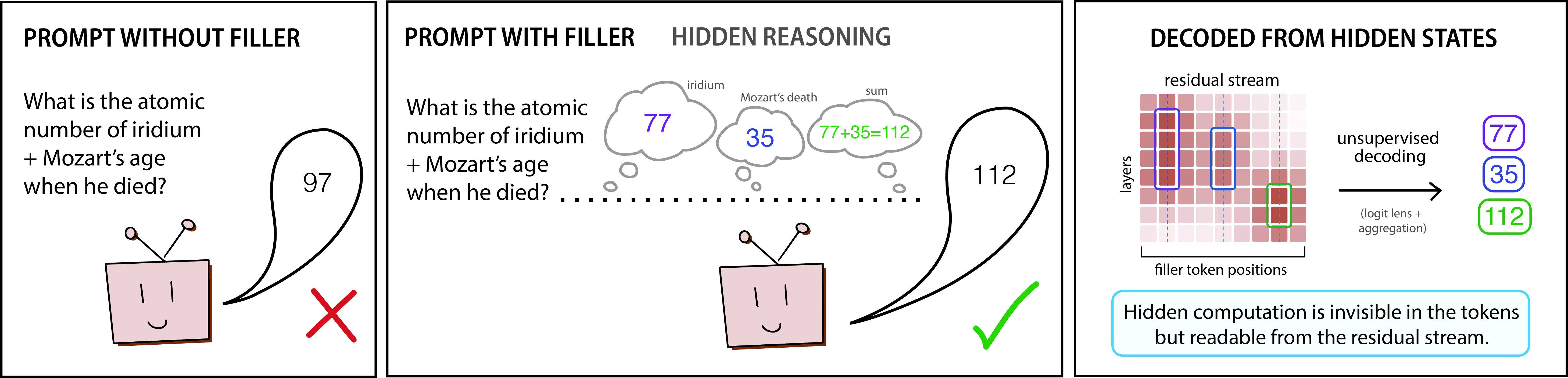
1.0.0.1 Contributions.
This paper moves from establishing a phenomenon, to localizing its mechanism, to recovering its content (Figure 1). Each step depends on the previous one. We make three contributions.
(1) Hidden computation over filler tokens is a general phenomenon. Prior work documented filler uplift in commercial frontier models on multi-hop problems [4], [5]. We show the phenomenon is broader than previously documented: open-source models DeepSeek V3 and Kimi K2 benefit from filler tokens on 1-fact addition (54% \(\to\) 72% on DeepSeek V3), 2-fact addition (21% \(\to\) 24% on DeepSeek V3, with 9% of examples flipping wrong\(\to\)right; 27% \(\to\) 35% on Kimi K2), 2-hop letter position (61% \(\to\) 70% on DeepSeek V3; 69% \(\to\) 75% on Kimi K2), and a system of equations (31% \(\to\) 61% on DeepSeek V3; 18% \(\to\) 36% on Kimi K2). Different filler types (dots, counting sequences, alphabet sequences) all provide similar uplift while scrambled sequences underperform, indicating that what matters is the presence of any non-disruptive token sequence, not any specific content.
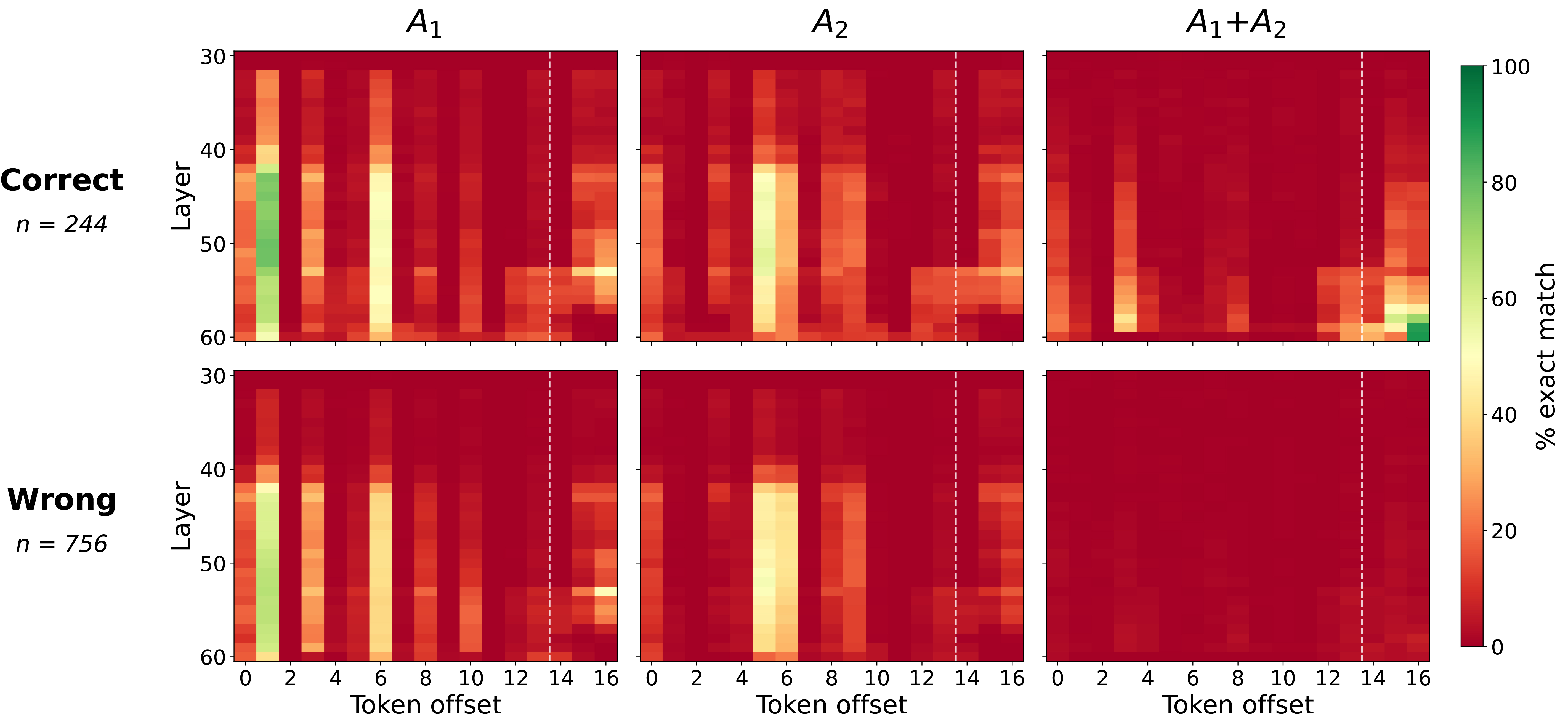
(2) Filler positions causally carry task-relevant information and encode the intermediate computation steps. We provide three lines of evidence. Attention analysis shows that when filler is present, the model redistributes its attention to form a processing relay of question \(\to\) filler \(\to\) answer that replaces the answer’s direct line to the question. Logit-lens readouts at filler positions reveal what the filler region encodes: across tasks and models, the intermediate values of the computation appear in the residual stream. In 2-fact addition, \(A_1\) is encoded strongly early in the filler, \(A_2\) later, and the sum \(A_1{+}A_2\) crystallizes in late layers immediately before the answer. KV-cache transplants at only the filler-token rows then establish that this content is causal: transplanting the filler region between matched examples drives the donor’s answer up by tens to hundreds of ranks, for retrieved facts and for values computed in context, and transplanting only the positions where an addend is decoded recovers most of the effect while the complementary positions carry almost none. The positional structure of the encoding is thus itself causal for the answer.
(3) An unsupervised pipeline recovers intermediate values from filler hidden states. We apply the logit lens at every (layer, filler position), subtract the cross-example mean to remove artifacts, aggregate residual scores across positions, and hand the top-50 tokens to an LLM judge for interpretation. The pipeline requires no ground-truth labels and no training. It recovers retrieved facts, parallel numeric intermediates, string-valued intermediates (element and city names), and in-context-computed values (system of equations) with 80–95% accuracy with the strongest LLM judge across both models and all four task families.
Across both models and all four tasks, the behavioral, mechanistic, and decoding results all show that filler tokens carry real computation and we can recover it from hidden states without supervision on these tasks. Code and aggregated decoding outputs are available at https://github.com/kaleybrauer/filler-token-reasoning.
2 Related work↩︎
2.0.0.1 CoT faithfulness and monitorability.
A growing literature establishes that chain-of-thought traces can fail to reflect the factors driving model behavior. [6] showed that models produce plausible CoTs that omit biasing features inserted into few-shot examples; [7] extended this to realistic prompts without artificial bias, finding implicit post-hoc rationalization on comparison questions; and [8] found that even modern reasoning models often fail to verbalize prompt-injected hints they relied on, with reveal rates often below 20% in tested settings but substantially higher in others. [9] showed a related dynamic from the training side: strong optimization against a CoT monitor can produce obfuscated reward hacking where the model hides its intent inside CoTs that the monitor accepts. On the other side, [10] argue that for tasks where CoT is computationally necessary, models struggle to evade monitors without significant help, and propose monitorability rather than faithfulness as the operationally relevant property. [1] synthesize these threads into a call to preserve CoT monitorability as a fragile safety property. Filler-token computation is a concrete failure mode for this property because the surface form of the reasoning is completely unrelated to the computation.
2.0.0.2 Filler tokens and hidden computation.
[2] showed that replacing CoT with filler periods in commercial LLMs gave no benefit, suggesting off-the-shelf models do not use filler tokens. [3] clarified this was not an in-principle limitation: small transformers can learn to use filler tokens, but only with task-specific parallelizable CoT supervision. [11] found that pretraining with explicit pause tokens yields gains across benchmarks, while introducing them only at finetuning gives mixed results. [4], [5] overturned this view at frontier scale: recent LLMs (Gemini 2.5/3 Pro, Claude Opus 4/4.5) emergently benefit from filler tokens on multi-hop tasks without filler-specific training, with 300 counting tokens nearly doubling Gemini 3 Pro’s 3-hop accuracy (18% \(\to\) 34%). Filler positions are functionally distinct from attention sinks [12], which absorb excess softmax mass rather than carry information; our KV-cache transplants (Section 4) show filler content is causally example-specific. Our work extends the filler-token phenomenon to open-weights models and investigates what is being computed across filler regions.
2.0.0.3 Latent multi-hop reasoning.
A separate line of work probes whether transformers compose facts internally without writing intermediates. [13] find strong evidence that LLMs internally identify the intermediate bridge entity (e.g., Stevie Wonder) on prompts like “the mother of the singer of ‘Superstition’ is…,” though evidence for the second hop is weaker and varies across prompt types. [14] extend this under shortcut-controlled evaluation and find high latent composability for some bridge types but not others. [15] localize the mechanism: in two-hop queries, the bridge entity is resolved in early layers and the second hop in later layers, and a late-to-early hidden-state patch recovers the correct answer in up to 66% of previously incorrect cases. These works study latent composition without filler tokens; we study what additional structure appears when filler tokens are inserted as a substrate for additional computation.
2.0.0.4 Logit lens and residual-stream interpretability.
The logit lens [16] projects intermediate residual states through the model’s unembedding to obtain a token distribution at each (layer, position). Variants and refinements include tuned-lens [17], future lens [18], and the patchscope framework [19] which generalizes this idea by patching hidden states into a separate prompt that elicits an interpretation. Our pipeline uses the logit lens to surface candidate tokens but relies on cross-example residual subtraction to remove formatting noise and on an LLM judge to interpret. The result is an interpretation step that is robust to the noise in mid-layer logit lens readouts and that can name compositional intermediates (e.g., element or city names) rather than only single tokens.
3 Behavioral exploration of filler-token uplift↩︎
We first establish that filler tokens improve open-weights model performance across our four task families. The tasks are constructed so that each has well-defined intermediate value(s). We use \(A\) for a single retrieved fact value (1-fact addition), \(A_1, A_2\) for the two retrieved values in 2-fact addition, and X for a random two-digit addend supplied in the prompt. The intermediate computation we aim to recover is A (1-fact), the pair \(\{A_1, A_2\}\) and their sum \(A_1{+}A_2\) (2-fact), or a string-valued retrieved entity such as a city or element name (2-hop letter position). For the system of equations, the prompt defines several variables by linear relations and asks for a linear function of one of them; reached by the chain \(x \to c_1 x \to y \to c_2 y \to \text{answer}\).
1-fact addition. “What is (fact A) plus (random two-digit \(X\))?”
2-fact addition. “What is the atomic number of (element \(A_1\)) plus the atomic number of (element \(A_2\))?”.
2-hop letter position. “What is the Nth letter of the capital of X?” (or of the chemical element with atomic number \(X\))
System of equations. “If \(\mathtt{ab}{=}51\); \(\mathtt{ce}{=}87\); \(\mathtt{da}{=}2\mathtt{ab}{-}21\); … what is \(3\mathtt{da}{-}79\)?” Several nonsense variables (including distractor variables) defined by linear relations over earlier ones, with every intermediate computed in context rather than retrieved.
We evaluate DeepSeek V3 and Kimi K2. For each task, the prompt has the form [question] [filler] Answer:. We vary the filler type (dots: “. . . . .”; counting: “1 2 3 4 5”; alphabet: “a b c d e”; and
scrambled variants c-scram, a-scram) and vary the filler length \(k\). We use 5 few-shot examples that themselves contain filler. For full task details and example prompts, see Appendix 9. The number of filler tokens \(k\) counts appended dots/numbers/letters, not model tokens; tokenization differs by filler type (e.g., "5 " is two tokens, ". " is one).
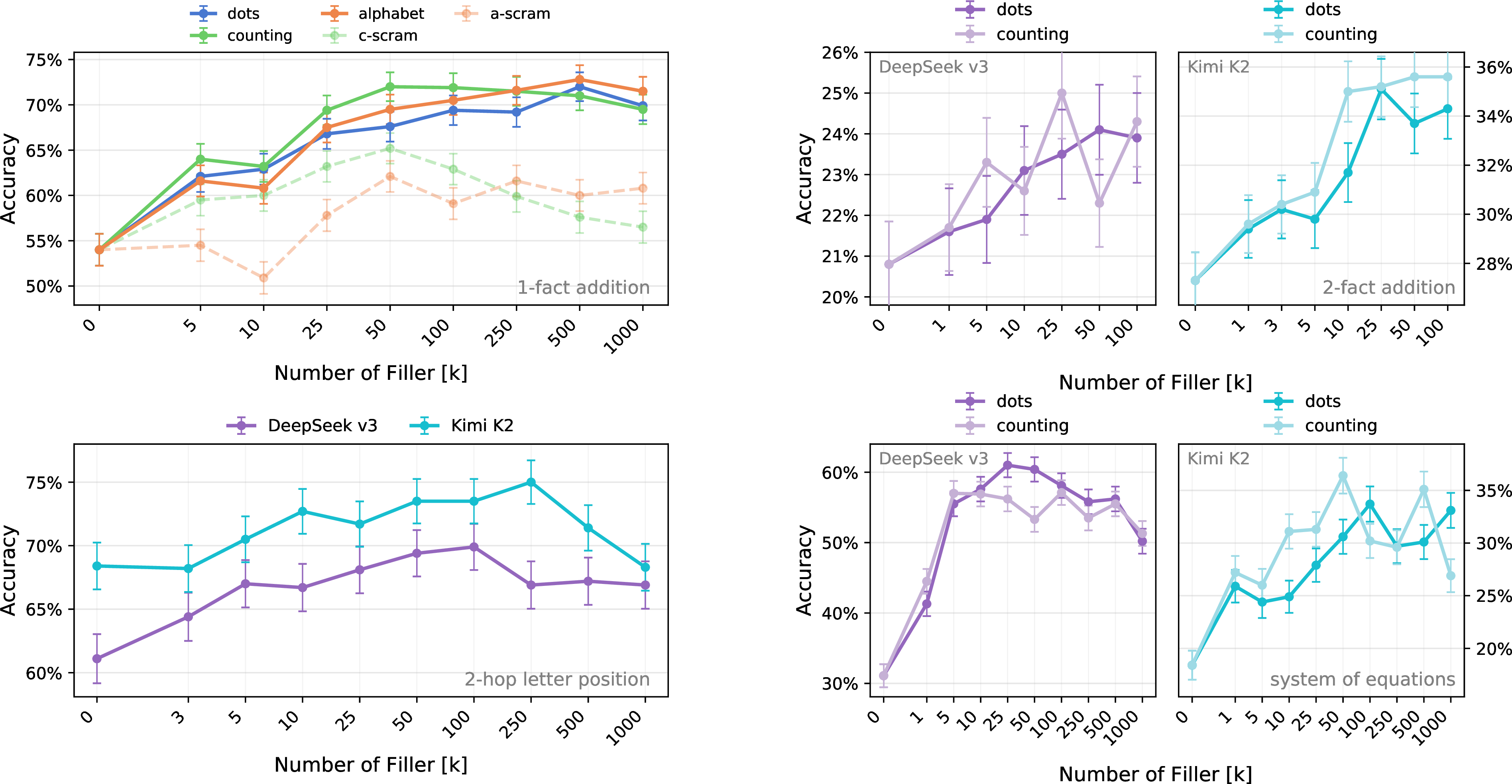
Figure 2 shows the results. On 1-fact addition, DeepSeek climbs from a 54% baseline to \(\sim\)72% with 100–500 dots/counting/alphabet tokens; scrambled fillers plateau \(\sim\)10% lower. On 2-fact addition, DeepSeek climbs from 21.1% to 24.1% with 50 dot tokens, and Kimi climbs from 27.3% to 35.6% with 50 counting tokens. On 2-hop letter position, dot and counting filler both lift DeepSeek from 61% to 70%, with comparable gains for Kimi. On the system of equations, DeepSeek V3 climbs from 31.1% to 61.0% and Kimi K2 from 18.4% to 36.4%, with every filler length giving a statistically significant uplift over baseline. Although DeepSeek’s net 2-fact uplift is small, filler enables \(\sim\)9% of examples to flip from wrong to right (counting filler: 135 wrong \(\to\) right out of 1500; McNemar \(p \approx 5 \times 10^{-4}\), [20]). The uplift is robust to whether the model was evaluated with API or locally with quantization (see Appendix 10). We also evaluated Qwen 3 480B which shows a small consistent increase on letter-position (43% \(\to\) 47%) but not addition, indicating filler-token computation is broader than previously documented but not universal even among comparably-scaled MoE models. Filler tokens placed before the question do not give uplift on these tasks; observed uplift requires filler between the question and answer.
The behavioral picture is consistent with what [4] found with commercial frontier models on harder tasks: smooth, length-dependent uplift from filler tokens. We additionally find sensitivity to disruptive filler sequences and observe diminishing returns at very long lengths.
4 Mechanistic evidence that filler encodes task-relevant information↩︎
What do filler positions encode, and how does the model use them? We provide three lines of evidence: the model forms a processing relay of question \(\to\) filler \(\to\) answer that routes information to the answer-forming position (attention); filler positions encode the intermediate computation steps in their residual stream (logit lens); and the content held at filler positions is causal for the answer (KV-cache transplants). For these analyses, we used local 4-bit quantized versions of DeepSeek V3 and Kimi K2 after verifying filler token uplift. For full details of the quantized models and the computational requirements, see Appendix 10 and 11.
4.1 Attention↩︎
When filler is present, the model shifts attention from the question to the filler tokens, which in turn attend to the question and to one another. In both baseline (no filler) and filler conditions, the answer position devotes \(\sim\)70–90% of its attention to the system prompt and few-shot examples, leaving \(\sim\)20% as the intermediate-computation routing budget. This is where filler shifts attention. In baseline, for DeepSeek V3, attention from the answer position to the question peaks at 15.8% at layer 40. With filler, at the answer position, attention to the question drops to 3–4% at the same layer, and the freed budget is redirected to the filler region: 13% for \(k=10\), rising to 18% for \(k=100\). Within the filler, late filler positions attend to earlier filler positions at 19–23% at layer 40 (robust across short and long fillers) and filler positions read from the question at 5–12% in middle layers. The displacement pattern is consistent across the L30–L50 mid-band. The picture is a processing relay of question \(\to\) filler \(\to\) answer with the answer’s direct line to the question replaced by a routed path through the filler region.
4.2 Logit lens reveals encoded intermediates↩︎
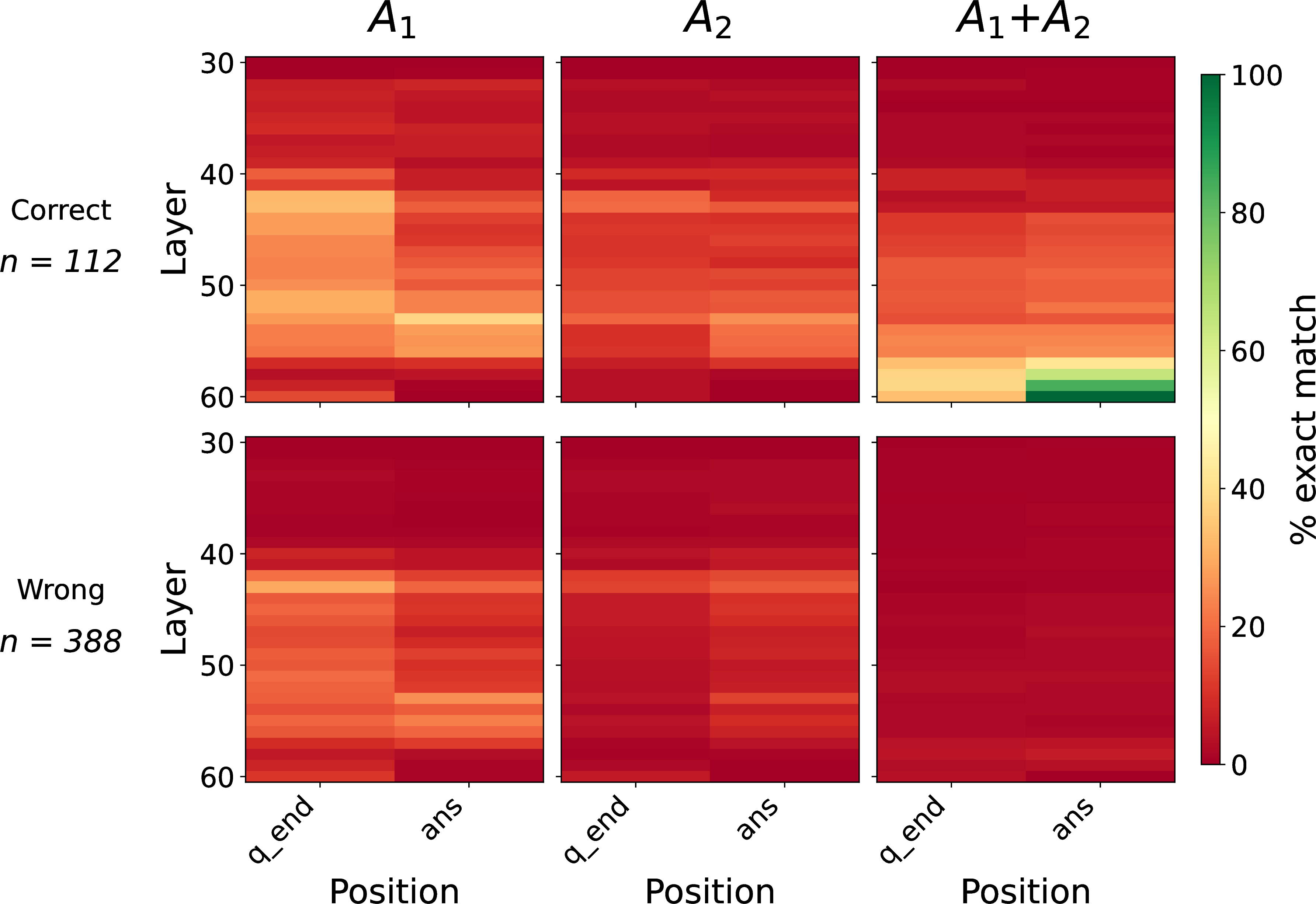
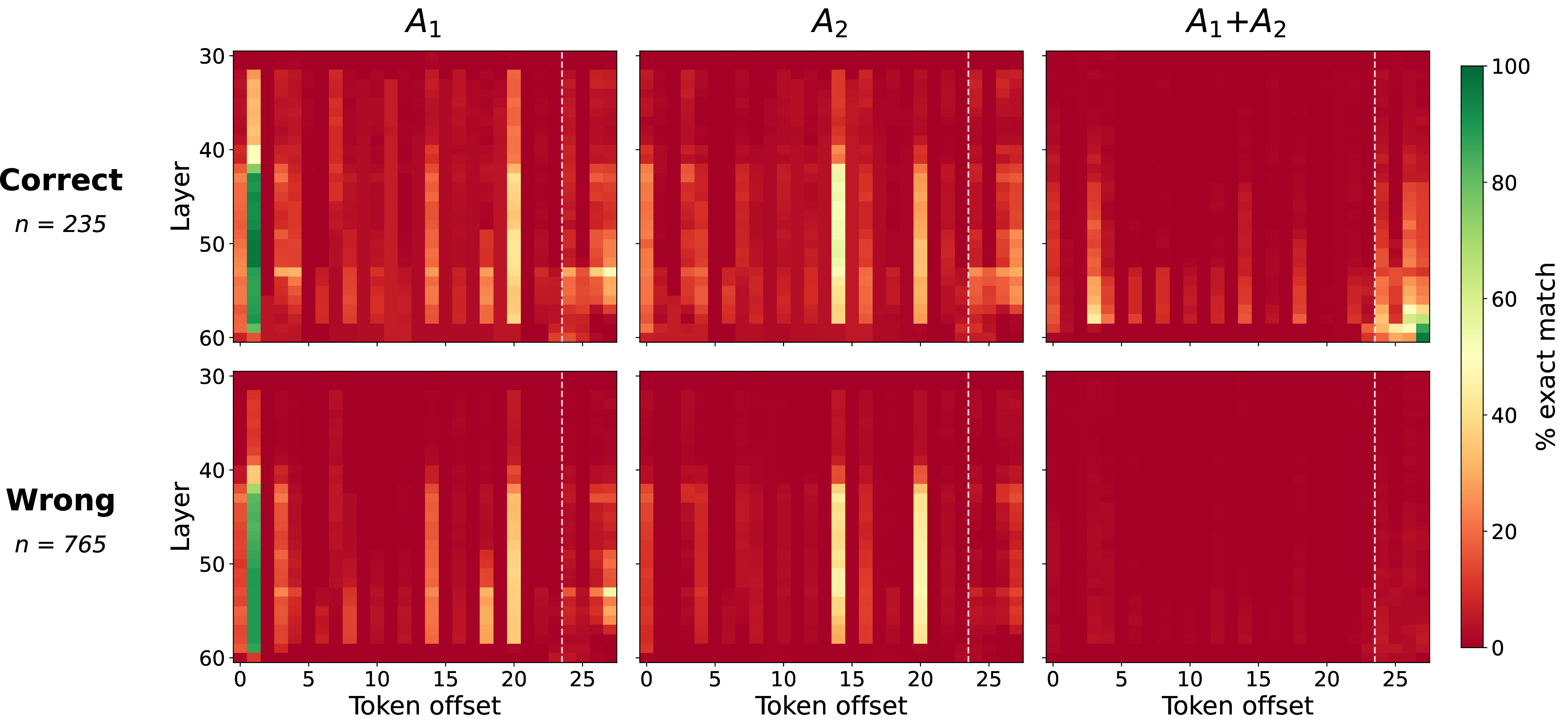
Filler positions encode task intermediates (\(A_1\), \(A_2\)) directly in their residual stream. We show this by projecting the residual at every (layer, filler position) through the model’s RMSNorm and unembedding, restricting to numeric tokens, and asking: how often is the top numeric token exactly equal to the ground-truth intermediate? Figure 3 shows the answer for 2-fact addition on DeepSeek V3 with \(k=10\) dot filler.
Across all examples, \(A_1\) is most strongly encoded in the first few filler tokens while \(A_2\) appears later. In correct examples, the sum \(A_1{+}A_2\) then appears in the last layers just before the answer position. The no-filler baseline has only the question-end and answer positions, with no filler region between them; there the sum \(A_1{+}A_2\) is strongly decoded value at the answer position (for correct examples; Appendix 12), while \(A_1\) and \(A_2\) decode weakly and do not appear clearly separated like in filler. In wrong filler examples, the sum is absent while \(A_1\) and \(A_2\) remain encoded: the model fails not by failing to retrieve, but by failing to compose. Decoding the residual stream thus reveals not just what the model thought, but also where its reasoning failed. Figure 3 shows results only for DeepSeek V3 dot filler with \(k=10\), but results are similar across longer filler lengths, different filler types, and both models (Appendix 12).
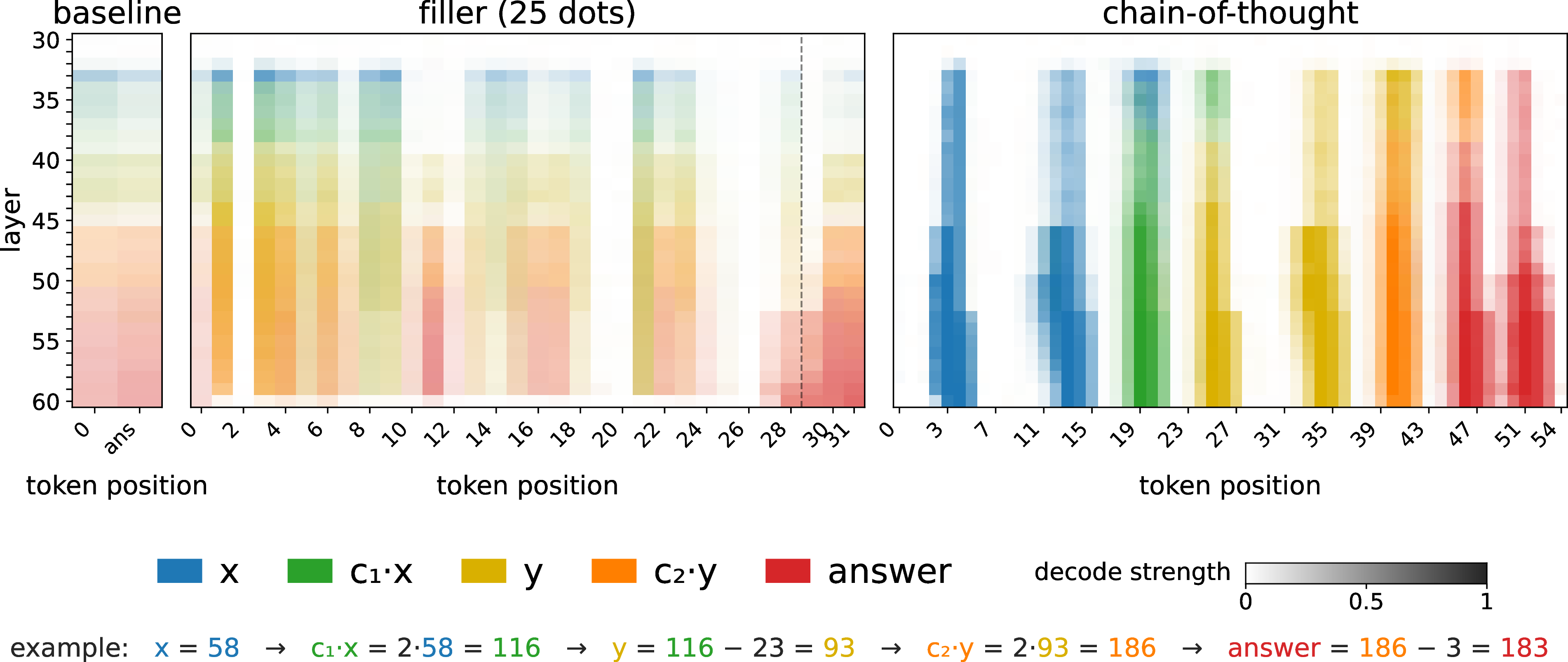
The same logit-lens readout also lets us compare how a computation is laid out under filler versus under an explicit chain-of-thought. Figure 4 does this for the system-of-equations task on DeepSeek V3, aggregating 500 examples in each of three conditions: no filler, 25 dots of filler, and explicit written reasoning (with all few-shot examples showing a consistent reasoning format so that the written steps fall at consistent positions across examples). Under filler, the intermediates of the chain (\(x\), \(c_1 x\), \(y\), \(c_2 y\), answer) are encoded across the filler positions in the same depth order in which the no-filler baseline forms them in a single pass at the answer position. This is true across different filler types and lengths. Under explicit chain-of-thought, each intermediate instead surfaces directly before the token position where it is written out. Aggregated across these 500 examples, the filler residual stream resembles the model’s ordinary single-pass computation spread across the available positions more than it resembles a written step-by-step derivation.
4.3 KV-cache transplants↩︎
The model attends to filler positions and encodes intermediate values there; we now show it causally relies on that content. Our KV-cache transplant is a form of activation patching, a standard tool in mechanistic interpretability for testing whether specific hidden states causally carry information [21]–[24]. On 1-fact addition, we run the model on 500 pairs of examples that share the addend \(X\) but differ in the underlying fact \(A\), and transplant the donor’s KV cache at only the filler-token positions into the target’s forward pass. For \(k=100\) dots, the donor’s \(A{+}X\) answer rank drops from 96\(^{+12}_{-15}\) (values reported with 95% CIs) in the unmodified target to 11\(^{+2}_{-3}\) after transplant. The effect holds for dots and counting filler (\(k=10-100\)) and is stronger for longer filler, as the model attends more to it. Full answer swaps (the target outputs the donor’s \(A{+}X\)) occur 13\(^{+3}_{-2}\)% of the time for dots \(k=100\), rising to 22\(^{+10}_{-7}\)% when the donor was correct and the target incorrect.
The same causal dependence holds when the value in the filler is computed rather than retrieved. For the system-of-equations task, we transplant the donor’s filler KV (again \(k=100\) dots) on 409 matched pairs that share the question’s arithmetic but differ in \(y\), so that adopting the donor’s \(y\) would make the target emit the donor’s answer. The donor-answer rank again drops sharply, from 236\(^{+47}_{-35}\) to 15\(^{+5}_{-3}\). The transplant changes the target’s answer 34.7\(^{+4.7}_{-4.4}\)% of the time; in 6.4\(^{+2.4}_{-2.2}\)% of cases the model outputs the donor’s answer outright (vs.% for 1-fact). Most changes corrupt the target’s own answer rather than fully swap it, but a patch confined to the filler positions, driving the donor’s specific answer up by hundreds of ranks, establishes that filler-position content is causal for the final answer.
The 2-fact task lets us test whether the positional structure of the encoding is itself causal, not just whether the filler region carries the answer. The logit lens (Figure 3) shows \(A_1\) and \(A_2\) each most strongly decode at distinct filler positions; we test whether those positions selectively control their addend. We build fact-matched pairs that hold one addend fixed and vary the other, so any answer shift is attributable to the varied addend. For \(A_1\) (\(n=405\), \(k=50\) dots), transplanting the whole filler region drops the donor answer’s rank from 88 to 18 (a shift of 70\(^{+15}_{-9}\) places), and transplanting only the 12 positions where \(A_1\) is decoded in \(\geq 15\%\) of examples (see Appendix 12) recovers 65\(^{+11}_{-11}\) of those 70 ranks (93%), while the 41 complementary positions move the rank by just 12\(^{+4}_{-3}\) and never swap (0.0%); \(A_2\) behaves the same (16 positions recover 49\(^{+14}_{-11}\) of 58 ranks, 85%). Full results are in Appendix 13. Each addend is independently and positionally manipulable, so the positional structure is a causal feature of the computation, not a logit-lens artifact.
5 Unsupervised decoding pipeline↩︎
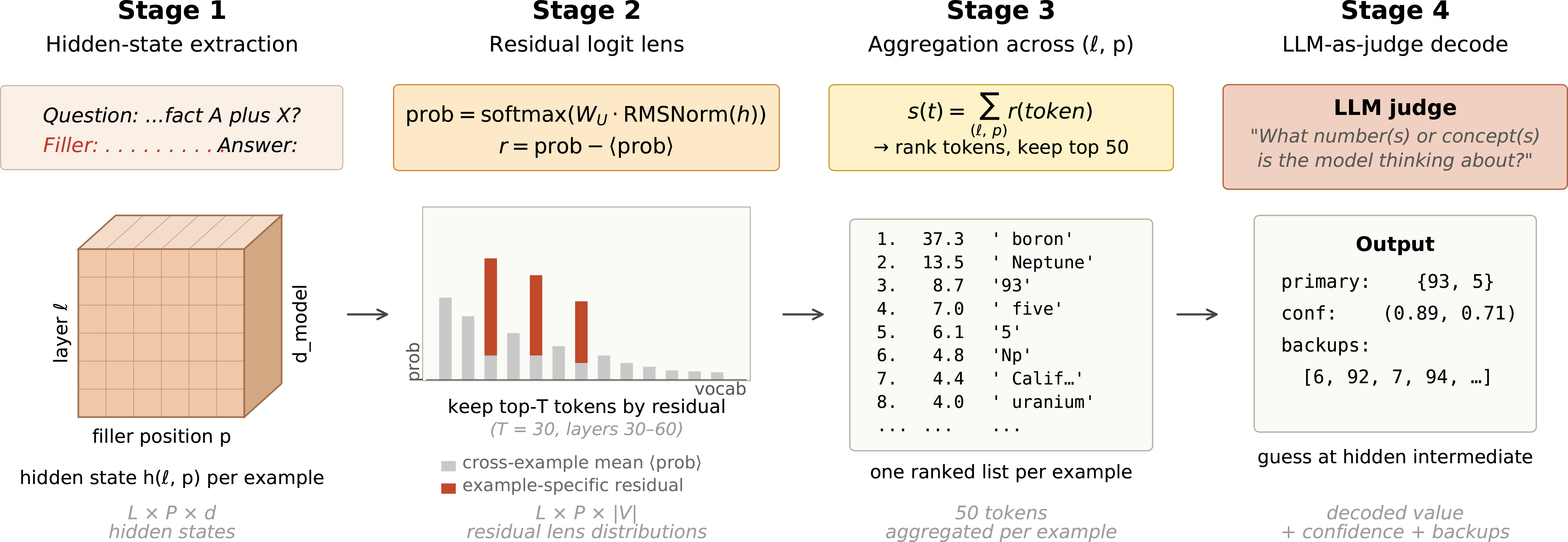
The heatmaps in Figure 3 require knowing the ground-truth intermediate. In a real white-box auditing setting, we would have only the model, the prompt, and the output when trying to discover what the model is computing. We now describe a pipeline, illustrated in Figure 5, that takes hidden states alone as input and produces a guess about the hidden reasoning being done, using no labels.
5.0.0.1 Stage 1: Hidden-state extraction.
For each example in a filler-task condition, we run the model and extract the residual stream at every transformer layer at every filler-token position. For DeepSeek V3 and Kimi K2, this is a \(\sim\)7000-dim vector for each of 60 layers for each token in the filler region.
5.0.0.2 Stage 2: Residual logit lens per (layer, filler position).
For a given (layer, filler position), we have hundreds to thousands of hidden-state vectors, one per example. We pass each through the model’s final RMSNorm and unembedding (the logit lens) to obtain a probability distribution over the full \(\sim\)129K-token vocabulary. We restrict analysis to layers in the second half of the model (layers 30–60 for both DeepSeek V3 and Kimi K2), where logit-lens readouts are more reliable.
We then compute, for each (layer, position), the cross-example mean probability for each token and define the per-example residual as the example’s distribution minus this mean. The residual step is not always necessary (see Section 6.5), but in general helps remove tokens that are always high (e.g., formatting artifacts) and keeps what is example-specific. We save the top-\(T\) tokens by residual score per example per (layer, position) (\(T=30\) by default).
5.0.0.3 Stage 3: Aggregation across filler positions.
We expect tokens related to the model’s computation to be encoded repeatedly across the filler region. For each example, we sum residual scores across all (layer, position) settings, rank tokens globally by this aggregated score, and keep the top 50. This pools both singularly strong and weak-but-consistent encodings into a single ranked list.
5.0.0.4 Stage 4: LLM decode.
The top-50 list contains the relevant intermediate(s) but is noisy and includes punctuation, partial subword tokens, and near-misses. We hand the list (with scores) to an LLM judge (Claude Haiku 4.5 and Claude Sonnet 4.6, separately) and ask, in a neutral prompt, what specific number(s) or concept(s) the model was reasoning about. For the full prompt provided to the LLM judges, see Appendix 14. The judge returns a primary guess and up to 10 backups. We score whether the true intermediate appears in the judge’s top-\(K\) predictions. For our results, we do not provide the original prompt and output to the LLM judge since it would make the judge’s job too easy, but in a real auditing setting this information could be provided to the judge for additional context.
Separately, we also evaluate without an LLM judge by checking whether the ground-truth intermediate appears among the aggregated top tokens directly. For numeric intermediates, we restrict to numeric tokens and check exact rank. For string intermediates, we use a top-\(K\) substring coverage measure that handles tokenizer splits and multiple languages (details in Appendix 15). This serves as a test of how much signal is in the top few tokens themselves versus how much benefit is added by the judge.
6 Decoding results↩︎
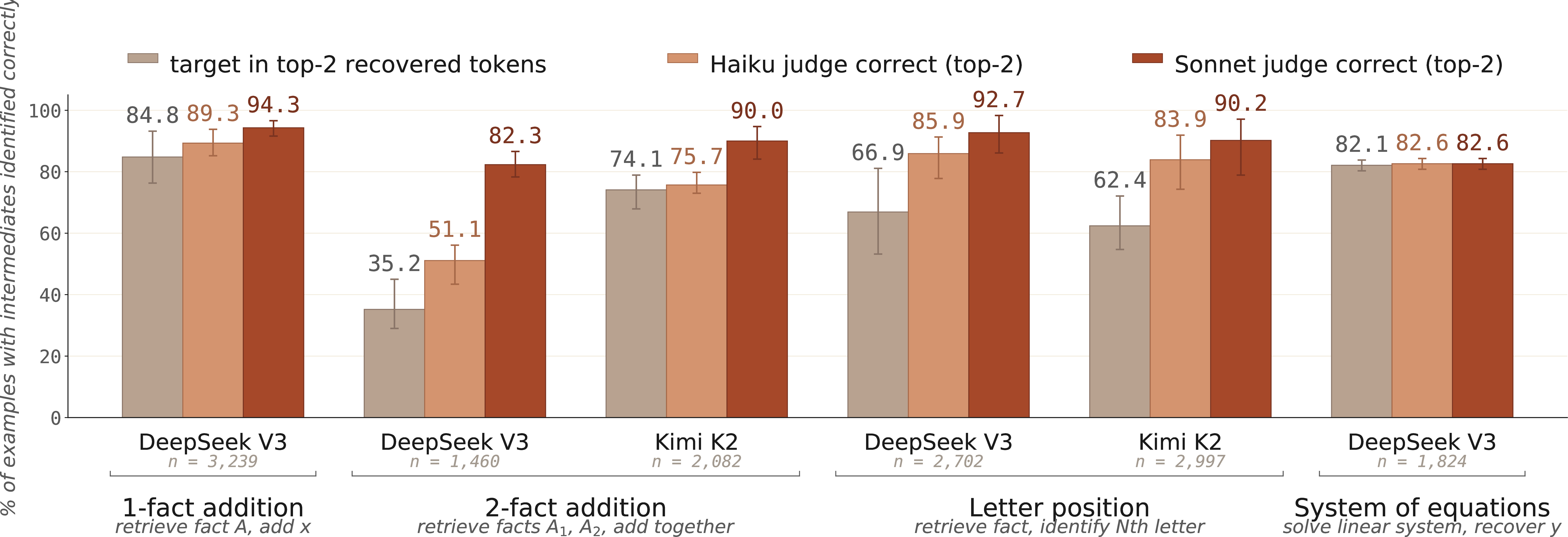
For each task–model combination, we report three numbers (Figure 6): the fraction of examples for which the ground-truth intermediate is in the top-2 decoded tokens after aggregation (no judge), the fraction for which a Haiku judge includes the target among its top-2 guesses after seeing the top-50 decoded tokens, and the same for a Sonnet judge. Throughout this section we report pooled accuracies across filler conditions; per-condition variation (min/max bars in Figure 6, full breakdown in Appendix 16) is generally within \(\pm5\) points. Here we score on correct examples because these are the cases with a well-defined target intermediate; the decoder runs identically on incorrect examples and reveals whether failures stem from missing retrieval or missing composition (Appendix 18).
6.1 A single retrieved value: 1-fact addition on DeepSeek V3↩︎
For 1-fact addition, the intermediate is the retrieved fact \(A\) (e.g., the age at which Mozart died). Pooling across nine filler conditions (\(n = 3{,}239\); dots, alphabet, and counting filler with \(k=5-100\)), the target appears in the top-2 numeric tokens after residual subtraction in 84.8% of examples, with no judge required. With Haiku as a judge, identification of the target rises to 89.3%; with Sonnet, 94.3%. Per-condition results (Appendix 16) show the same pattern across every filler type/length: Haiku top-2 ranges from 85.2% to 93.8%, and Sonnet top-2 from 91.6% to 96.6%.
6.1.0.1 Failures are structured, not noise.
The most common incorrect guess is the given addend \(X\) (the random two-digit number from the prompt), which appears as top-1 in 39–69% of these failure cases. The sum \(A{+}X\) appears in 16–29%. Direct neighbors (\(A \pm 1\), \(X \pm 1\), sum \(\pm 1\)) account for an additional few percent. In other words, when the pipeline fails to surface \(A\), it is almost always because the model is more strongly encoding \(X\) or the answer, not because it is outputting noise.
6.2 Two parallel intermediates: 2-fact addition↩︎
The 2-fact task is the most demanding of the three: the model must retrieve two intermediate values and combine them. Pooling DeepSeek V3 results across six filler conditions (\(n = 1{,}460\)), both \(A_1\) and \(A_2\) appear in the top-2 numeric tokens in 35.2% of examples. The Haiku judge raises identification of both targets to 51.1%, and Sonnet to 82.3%. On Kimi K2 (\(n = 2{,}082\)), the corresponding numbers are 74.1% / 75.7% / 90.0%. Kimi K2 is more accurate on the task and encodes the intermediates more cleanly.
The judge gap is much larger on this task than on 1-fact (DeepSeek 2-fact: 35.3 \(\to\) 82.3; DeepSeek 1-fact: 84.8 \(\to\) 94.3). The reason is that with two intermediates, the top-2 numeric tokens often miss one of them: in DeepSeek V3 dots-25 conditions, \(A_1\) appears in top-2 in 80% of examples but \(A_2\) only in 48%, so both-in-top-2 is only 31%. The judge, which sees the full top-50 list and can use context (e.g., relevant word tokens, identifying that two numbers add to another number), better recovers both intermediates.
6.2.0.1 Failures encode the partial computation.
When neither \(A_1\) nor \(A_2\) is in the top-2, the most common numeric token is the sum \(A_1 {+} A_2\) itself: for DeepSeek V3 dots-25, 41% of failures have the exact sum in top-2, and in 73% it is within \(\pm 5\). Combined with \(A_1 \pm 1\) and \(A_2 \pm 1\) near-misses, structured failure modes account for \(\sim\)60–80% of all failures. The model is partway through its computation and is representing the sum rather than the addends. This is not a pure failure as it is still related to the underlying computation.
6.3 Non-numeric intermediates: letter-position tasks↩︎
The decoding pipeline generalizes to tasks with words (typically represented by multiple tokens) as intermediates. For the letter-position task, the intermediate is a city or element name. For top-2 token scoring, we check whether the target appears among the top-2 decoded string tokens, allowing either English or Chinese matches (DeepSeek V3 and Kimi K2 frequently “think” in Chinese, e.g., [25], [26]; see Appendix 15 for details). On DeepSeek V3 (\(n=2{,}702\)), a match for the target appears in the top-2 string tokens for 66.9% of examples, Haiku reaches 85.9%, and Sonnet reaches 92.7%. On Kimi K2 (\(n=2{,}997\)), the corresponding numbers are 62.4% / 83.9% / 90.2%.
6.3.0.1 Prompt sensitivity.
We compare how different judge prompts affect results. A neutral prompt asks generically what the model was reasoning about; a task-specific prompt names the expected target type (“the name of a chemical element” or “the name of a city”). The task-specific prompt helps both judges where there is room to improve. On element names, Sonnet is already near ceiling under the neutral prompt and shows little change (\(\sim\)0%), while Haiku gains 3–6%. On city names, a harder subtask where neither judge is saturated, the city-aware prompt helps both, with Sonnet gaining up to 11% and Haiku gaining up to 13%. This suggests the unsupervised pipeline can be made more accurate when an auditor has a hypothesis about what kind of information to search for, but does not require one for simple, clearly-defined intermediates.
6.4 A computed intermediate: system of equations on DeepSeek V3↩︎
The previous three tasks all decode a retrieved fact; the system-of-equations task tests whether the pipeline also recovers a value the model must compute in context. The queried variable’s value \(y\) sits in the middle of a short arithmetic chain \(x \to c_1 x \to y \to c_2 y \to \text{answer}\), in which \(x\) is given in the prompt and the remaining quantities are formed in context. We score recovery of \(y\), the one intermediate that is itself a named variable (the sub-products \(c_1 x\) and \(c_2 y\) never appear as their own equation), which also keeps it comparable to the single-target retrieval tasks. Pooling DeepSeek V3 across six filler conditions (\(n=1{,}824\)), \(y\) appears in the top-2 numeric tokens in 82.1% of examples. Unlike the retrieval tasks, the judges add essentially nothing here (Haiku 82.6%, Sonnet 82.6%). The prompt is built from nonsense variable names and random numbers, so there is no surrounding context for a judge to exploit beyond the decoded tokens themselves. This is consistent with the pattern on the other tasks, where the judge’s gains come from contextual signal. The other intermediates (\(x\), \(c_1 x\), \(c_2 y\), and the answer) decode at varying rates, reflecting a deeper computation with more transient sub-products (full per-intermediate breakdown in Appendix 17).
6.4.0.1 “Failures” land on adjacent steps.
As on the other tasks, “failures” are structured. When \(y\) is not the top-1 token, the decode most often surfaces the adjacent step of the same chain: \(c_2 y\), the sub-product one rung below the answer, in 67% of these cases, and the answer itself in a further 14%; only 5% is off-problem. The pipeline often returns every step of the multi-step computation. Within the top-10 tokens, every step (\(x\) through the answer) is found 51% of the time (\(x\)) to 97% of the time (\(y\)).
6.5 Residual subtraction: when does it help?↩︎
We ablate the residual-subtraction step by re-running the pipeline with raw logit-lens probabilities instead of residualized scores. Results on DeepSeek V3 2-fact addition show that residualization can help substantially: with dots-10 filler, Sonnet top-2 accuracy is 82.4% with residualization versus 73.8% without, an 8.6 pp gain (see Appendix 19). However, residualization is not uniformly beneficial. With counting filler, it hurts the Haiku judge by up to 11.5 pp, from 90.6% to 79.1% at top-10. This is because counting digits are themselves often relevant intermediates and the residual step suppresses them. Residualization helps when: (i) there is a strong cross-example baseline obscuring the signal (formatting, common artifacts); (ii) the decode target varies across examples; and (iii) the downstream judge does not need the suppressed tokens. Where any of these breaks, raw logit-lens readouts may be preferable. We report residualized results as the default but note the trade-off.
7 Limitations↩︎
7.0.0.1 Logit-lens artifacts.
The logit lens is a coarse readout of the residual stream and is known to be unreliable in early layers and on tokenizer-level artifacts [16], [17]. We mitigate this by restricting to the second half of layers and aggregating across many positions, but a tuned-lens [17] might recover signal we miss. Additionally, all mechanistic and decoding analyses are run on 4-bit quantized checkpoints; while behavioral uplift is preserved under quantization and our KV-cache results provide lens-independent causal evidence, we cannot rule out that quantization affects residual-stream geometry in ways that influence logit-lens readouts specifically.
7.0.0.2 Partial but not full auditability.
Our pipeline targets tasks where there is a discrete, nameable intermediate value (a number, an element name, a city), and recovers these with 80–95% accuracy. Multiple failure modes lie outside this regime. The pipeline reads residual content via the logit lens and so requires the relevant computation to be expressible through the unembedding matrix; computation that lives in attention patterns or in directions orthogonal to the vocabulary projection would be invisible to it. Intermediates that do not correspond to a single tokenizable concept, such as a strategy or a goal (e.g., an intent to deceive), are harder but not necessarily out of reach. A sufficiently capable judge could in principle infer such concepts from the constellation of related vocabulary tokens that surface in the top-\(K\) list, much as our Sonnet judge already infers numeric intermediates from context when they are not in the top-\(2\). The harder cases are concepts whose related vocabulary does not surface in the top-\(K\) at all, or computation specifically optimized to look like benign token activity. Whether residual-stream decoding can be extended to such targets, perhaps via patchscope-style [19] elicitation or trained probes, is an important open question. Our claim is the weaker one that hidden filler computation is at least partially accessible to interpretability on tasks with clean intermediates.
7.0.0.3 The chain-of-thought comparison is qualitative.
The comparison between filler and explicit chain-of-thought in Figure 4 is a visual aggregate over 500 examples on a single task. It indicates that the filler residual stream resembles the model’s single-pass computation more than “hidden chain-of-thought”, but we do not reduce it to a single metric or claim the two are algorithmically identical.
7.0.0.4 Access to closed-weights models.
Our pipeline requires full hidden states, available only for open-weights models. Filler-token uplift has been documented in commercial frontier models [4], [5], and the consistency of our results across two frontier-scale architectures suggests the encoding pattern is not model-specific, but direct verification on Claude, Gemini, or GPT is not currently possible.
8 Discussion↩︎
The combined behavioral, mechanistic, and decoding evidence shows that filler positions read information from the question, hold and process intermediate values across the residual stream, and are read out by the answer position. For 2-fact tasks, the residual stream encodes \(A_1\) early in the filler, \(A_2\) later, and the sum in late layers just before the answer position. By reading the residual stream, we are also able to identify where the reasoning fails when the model answers incorrectly.
This has implications for CoT monitorability. Filler-token computation is considered a limit case where reasoning is performed in tokens whose surface form is uninformative [2], [3], and indeed as Sections 3 and 4 confirm, filler computation is real and not visible in the output text. But behavioral monitoring is not the only auditing tool available. Cheap interpretability tools (logit lens with cross-example normalization and an LLM judge) can recover most of the hidden intermediates on our tasks without supervision. The implication is not that CoT monitoring is safe, but that the gap is at least partially closable by reading the residual stream. Hybrid behavioral + interpretability auditing is more capable than either alone, and residual-stream access is a meaningful complement to surface-token monitoring.
Several open questions follow naturally from the picture above. First, at the circuit level: which attention heads implement the question \(\to\) filler \(\to\) answer relay, and do they overlap with heads used in explicit-CoT problem solving? Second, on harder intermediates: how far can the pipeline be extended to tasks where the relevant computation is not a single nameable token, possibly via trained probes or patchscope-style elicitation? Third, on adversarial robustness: can a model trained to use filler tokens evasively, e.g., to distribute its computation across the residual stream in ways the logit lens cannot read, still be decoded by a more sophisticated auditor?
Overall, pessimism about CoT monitorability is incomplete. Hidden computation, a concrete case where behavioral oversight fails, is at least partially accessible to interpretability on decomposable tasks. Opaque is not necessarily the same as unauditable.
Impact Statement↩︎
This work studies whether hidden computation in large language models, specifically multi-step reasoning performed across content-free filler tokens, remains accessible to interpretability tools when it is invisible to chain-of-thought monitoring. The intended contribution is to AI oversight. We show that on tasks with discrete, nameable intermediates, residual-stream decoding can complement behavioral CoT monitoring and partially close the gap created by unfaithful or opaque surface tokens. We see this as a positive-leaning impact for safety-relevant interpretability research. We do not identify direct negative societal impacts beyond those of interpretability research generally.
Supplementary Material↩︎
Supplementary material for the paper “Reading Between the Dots: Decoding Hidden Computation across Filler Tokens.”
This appendix collects experimental details and supplementary results that did not fit in the main text. In Appendix 9, we describe the four task families in detail, including fact sources, filtering and few-shot construction, the conditions evaluated, and full example prompts. In Appendix 10, we document the specific 4-bit quantized checkpoints of DeepSeek-V3 and Kimi K2 used throughout the paper, including which layers and projections are held at higher precision. In Appendix 11, we report the computational requirements of every experiment and pipeline stage (model loading, hidden-state extraction, KV-cache transplants, attention analysis, residual decoding, and LLM-as-judge calls) together with hardware and storage budgets. In Appendix 12, we provide baseline and additional logit-lens heatmaps showing that the encoding pattern observed for DeepSeek V3 with dot-10 filler in Figure 3 generalizes to Kimi K2, to counting filler, and to longer filler lengths. In Appendix 13, we report full results for the KV-cache transplants with 2-fact addition. In Appendix 14, we give the full prompts shown to the LLM judges (Claude Haiku and Claude Sonnet), in both the neutral and task-specific framings discussed in Section 6. In Appendix 15, we define the multilingual top-\(K\) substring-coverage measure used to score string-valued intermediates without an LLM judge. In Appendix 16, we report the full top-\(K\) decoding results for all tasks, models, filler conditions, and judges. We also provide shuffled-token baseline controls that show judge performance is not merely prompt-induced guessing. Appendix 17 gives the full per-intermediate decoding breakdown for the system-of-equations task. In Appendix 18, we provide the decoding results for incorrect examples and investigate failure modes. Finally, in Appendix 19 we ablate the residual-subtraction step used in the main decoding pipeline and show that it can be significantly beneficial but not always.
9 Task information and example prompts↩︎
1-fact addition
Types of facts: Facts are drawn from Ryan Greenblatt’s compose_facts repository.1
125 age facts (age at which famous person died; range 20–97);
118 atomic number facts (range 1–118);
76 static facts (generic facts like vertebrae count, opera counts, alphabet sizes; range 6–600)
Fact filtering and few-shot: When creating the 1-fact addition dataset, we first check that the model (DeepSeek V3 or Kimi K2) knows the answer when asked as a standalone question. Any fact not answered correctly at least 3/4 times is filtered out of the dataset. Then, 5 facts are randomly excluded from the dataset to serve as few-shot examples. Each prompt uses the same 5 few-shot examples.
Task format: What is <fact A> plus <random 2-digit addend X>?
Conditions: dot filler with \(k=10, 25, 50\); counting filler with \(k=5, 10, 25\); alphabet filler with \(k=10, 25, 50\)
Example prompt: For dots, \(k=10\). The system prompt is slightly varied for each condition to reflect the correct filler type and length.
### system
You will be given a question. Answer immediately using the format ‘Answer:’ where [ANSWER] is just the number, nothing else. No explanation, no words, no reasoning, just the number. After the question, there will be 10 filler tokens (a sequence of dots)
before you answer.
### user
Question:What is the age at which Søren Kierkegaard died plus 96?
Filler:.......…
Answer:
### assistant
138
### user
Question:What is the age at which Elizabeth I of England died plus 40?
Filler:.......…
Answer:
### assistant
109
[... more few-shot pairs (Coltrane / oxygen / phosphorus)...]
### user
Question:What is the atomic number of silicon plus 62?
Filler:.......…
Answer:
2-fact addition
Types of facts: 100 atomic number facts (range 1–100)
Fact filtering and few-shot: Because this task is much more difficult than 1-fact addition, we restrict to only atomic number facts \(\leq100\). 10 facts are randomly excluded from the dataset to serve as few-shot examples. Each prompt uses the same 5 few-shot examples.
Task format: What is the atomic number of <element A1> plus the atomic number of <element A2>?
Conditions: dot filler with \(k=10, 25, 50\); counting filler with \(k=10, 25, 50\)
Example prompt: Same format as 1-fact addition.
2-hop letter position
Types of facts:
367 capitals of countries/states/provinces/territories
- includes all countries, US states, Chinese provinces/autonomous regions, Indian states, Brazilian states, German states, Canadian provinces/territories, Mexican states, and Australian states/territories that do not share all or most of their name with their capital city
100 chemical element facts
- includes all chemical elements from 2-fact addition dataset, inverted to ask for the element name instead of atomic number
Fact filtering and few-shot: 5 facts are randomly excluded from the capitals dataset and from the chemical elements dataset to serve as few-shot examples. Each prompt uses the same 5 few-shot examples.
Task format: What is the <second/third/last> letter of the chemical element with atomic number <A>?; What is the last letter of the name of the capital of <country/state/province/territory>?
Conditions: dot filler with \(k=10, 25, 50\); counting filler with \(k=10, 25, 50\)
Example prompt: Same format as 1-fact addition, except with system prompt modified to say letter instead of number:
### system
You will be given a question asking for a specific letter. Answer immediately with just the single lowercase letter, nothing else. No explanation, no words, no reasoning, just the letter. After the question, there will be 10 filler tokens (a sequence of
dots) before you answer.
[5 few-shot examples ...]
### user
Question: What is the third letter of the chemical element with atomic number 47?
Filler: . . . . . . . . . .
Answer:
System of equations
Motivation: The other three tasks use a retrieved fact as the intermediate. The system-of-equations task instead makes every intermediate a value computed from numbers given in the prompt, with nothing to retrieve.
Task structure: Each prompt assigns a few nonsense variables literal two-digit values (0–99) and defines others as linear functions of an earlier variable (multiply by a constant of 2 or 3, then add or subtract a constant from 0–50). The question asks for a linear function of one variable. Distractor variables that do not feed the queried variable are included, so the model must bind the correct names rather than the most recent numbers. We write the queried variable’s value as \(y\), reached by the chain \(x \to c_1 x \to y \to c_2 y \to \text{answer}\), where \(x\) is the in-context value it depends on.
Conditions: dot filler with \(k=10, 25, 50\); counting filler with \(k=5, 10, 25\).
Example prompt (dots, \(k=10\); queried variable cad, giving \(x{=}\texttt{bec}{=}50 \to c_1 x{=}100 \to y{=}\texttt{cad}{=}79 \to c_2 y{=}158 \to
\text{answer}{=}129\)):
### system
You will be given a list of variable definitions and a question. Answer immediately with just the number, nothing else. No explanation, no words, no reasoning, just the number. After the question, there will be 10 filler tokens (a sequence of dots) before
you answer.
[5 few-shot examples ...]
### user
aba = 93
bec = 50
dab = three times the number for bec plus 20
cad = two times the number for bec minus 21
bah = three times the number for cad minus 44
Question: What is two times the number for cad minus 29?
Filler: . . . . . . . . . .
Answer:
Easier variation for Kimi K2: At this task, DeepSeek V2 has significantly higher base accuracy than Kimi K2. To create headroom for measuring behavioral uplift in Kimi K2 (Figure 2), we made the task slightly easier in two ways: we fixed every coefficient to 2 (rather than drawing from \(\{2, 3\}\)) and drew the additive/subtractive constants from \(1\)–\(30\) (rather than \(1\)–\(50\)). All other parameters (five variables, a single chained reference, and literal values in \(10\)–\(99\)) were unchanged.
10 Models↩︎
We evaluate two pretrained instruction-tuned models. They are run from publicly-available 4-bit quantized checkpoints to fit available GPU memory.
DeepSeek-V3 (4-bit AWQ).
We use cognitivecomputations/DeepSeek-V3-0324-AWQ, a 4-bit AWQ [27] quantization of DeepSeek-V3-0324 [28]. The base model is a 671B-parameter Mixture-of-Experts model with \(\sim\)37B parameters activated per token. AWQ is applied with group
size 128, asymmetric (zero-point) quantization, and the GEMM kernel; the multi-query attention KV projection (self_attn.kv_a_proj_with_mqa) is held at FP16.
Kimi K2 (W4A16).
We use Red Hat / Neural Magic’s Kimi-K2-Instruct-quantized.w4a16, a 4-bit-weight / FP16-activation quantization of Moonshot AI’s Kimi-K2-Instruct [29]. The
base model is a 1T-parameter Mixture-of-Experts model with \(\sim\)32B parameters activated per token. Quantization (compressed-tensors format) targets only the routed-expert FFN linears: weights are int4 with symmetric
per-group quantization (group size 128), and lm_head, all self-attention projections, the shared experts, and the MLP gate``up/down projections are held at FP16.
11 Computational requirements↩︎
All experiments are run on a single workstation with 3–4 NVIDIA H200 (150 GB HBM3) GPUs.
Full code and aggregated results are available at https://github.com/kaleybrauer/filler-token-reasoning. To make the analysis reproducible without requiring readers to rerun the full decoding pipeline, we release the main intermediate and summary outputs used in the paper: per-example aggregated top-50 residual tokens, Claude judge responses, top-\(K\) accuracy tables, and logit-lens heatmap summaries. These artifacts cover the correct-example subset across the filler conditions, judges, prompts, and model.
Model loading. DeepSeek V3 (4-bit AWQ) is loaded across 3 H200s with \(\sim\)110–130 GB allocated per GPU. Kimi K2 (4-bit W4A16) is loaded via vLLM with tensor parallelism degree 4 on 4 H200s.
Hidden-state extraction. For each model and each condition, we run forward passes with hidden states cached at every transformer layer and every prompt-relative token offset, then write per-example pickles to disk. Per example, per condition: 61 layers \(\times\) \(\sim 10-100\) positions \(\times\) float16 hidden state (\(d_{\text{model}}=7168\)) per example \(\approx\) 50 MB / example, \(\approx\) 50 GB / condition. Cumulative extraction cache for all examples across all tasks for both models is \(\sim\)1 TB.
KV-cache transplant. For each donor/target pair, we run prefill twice, splice the donor’s filler-region key-value cache into the target’s KV state at every layer, and decode the next token. We use 500 random pairs per filler condition on the 1-fact addition task. The intervention runs with quantized DeepSeek V3 on the same 3-H200 setup as extraction.
Attention analysis. Filler-attention summaries aggregate per-head attention weights at every (layer, source-position, target-position) intersection on 100 examples per condition for the 1-fact addition task and a no-filler baseline. Per-example attention matrices are reduced on the fly into the segment-level breakdown (system / few-shot / question / filler / answer-label) reported in the paper.
Residual decode. Residual fingerprints (per-(example, layer, position) top-50 token IDs after subtracting the cross-example mean softmax distribution) are computed offline by streaming through the cached hidden states with the same RMSNorm + lm_head used at inference. This step can be run on CPU and runs in tens of minutes per condition.
LLM-as-judge decoding. Top-50 residual tokens are scored by Claude Haiku 4.5 and Claude Sonnet 4.6 via the Anthropic API. We issue \(\sim\)6 (conditions) \(\times\) \(\sim\)250–360 (examples) \(\times\) 2 (judge models) \(\times\) 2 (prompt framings: neutral and task-specific) calls per task, totaling \(\mathcal{O}(10^4)\) API calls per task across DeepSeek V3 and Kimi K2.
Storage. Quantized model weights occupy \(\sim\)840 GB on local SSD; intermediate extraction caches occupy \(\sim\)1 TB; final aggregated residual JSONs and judge outputs occupy \(<\)5 GB.
12 Logit-lens heatmaps↩︎
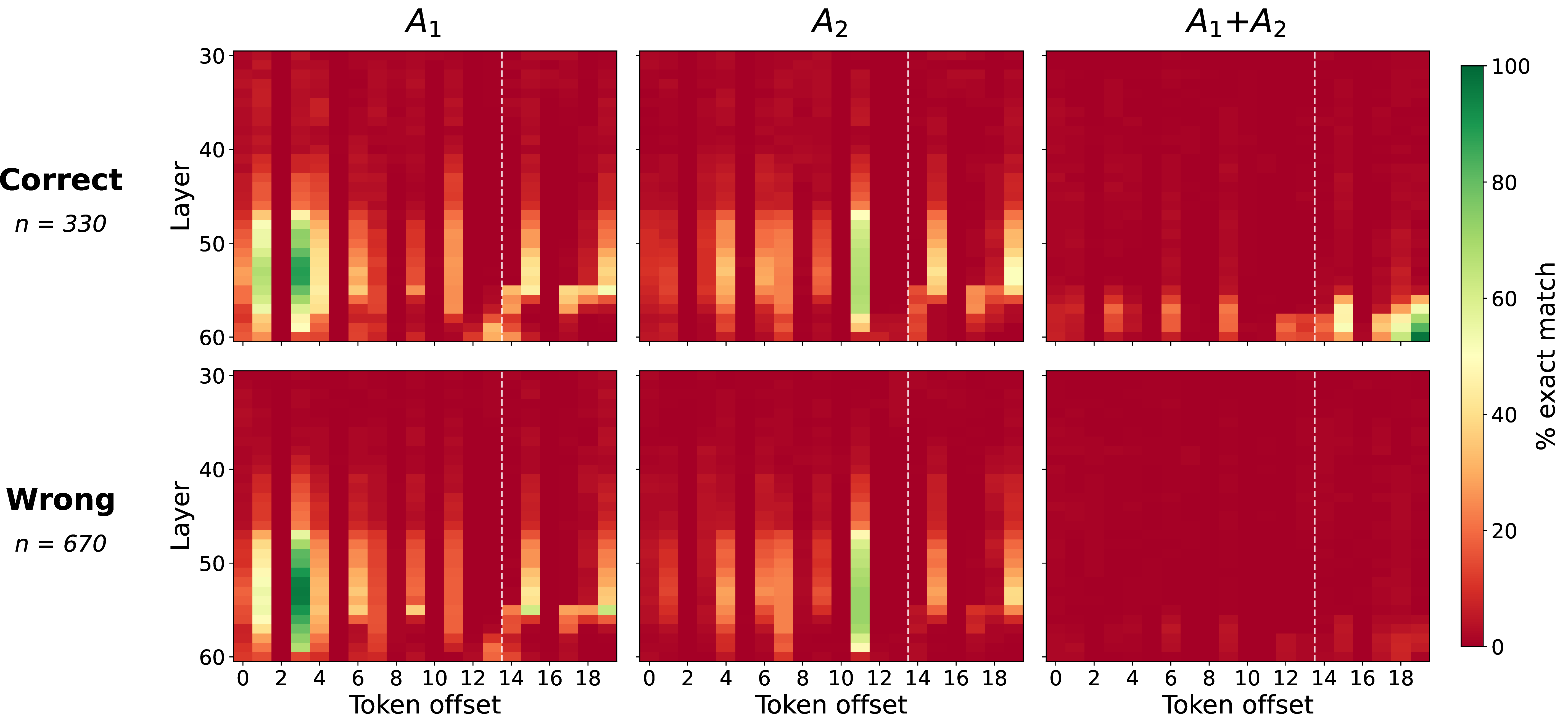
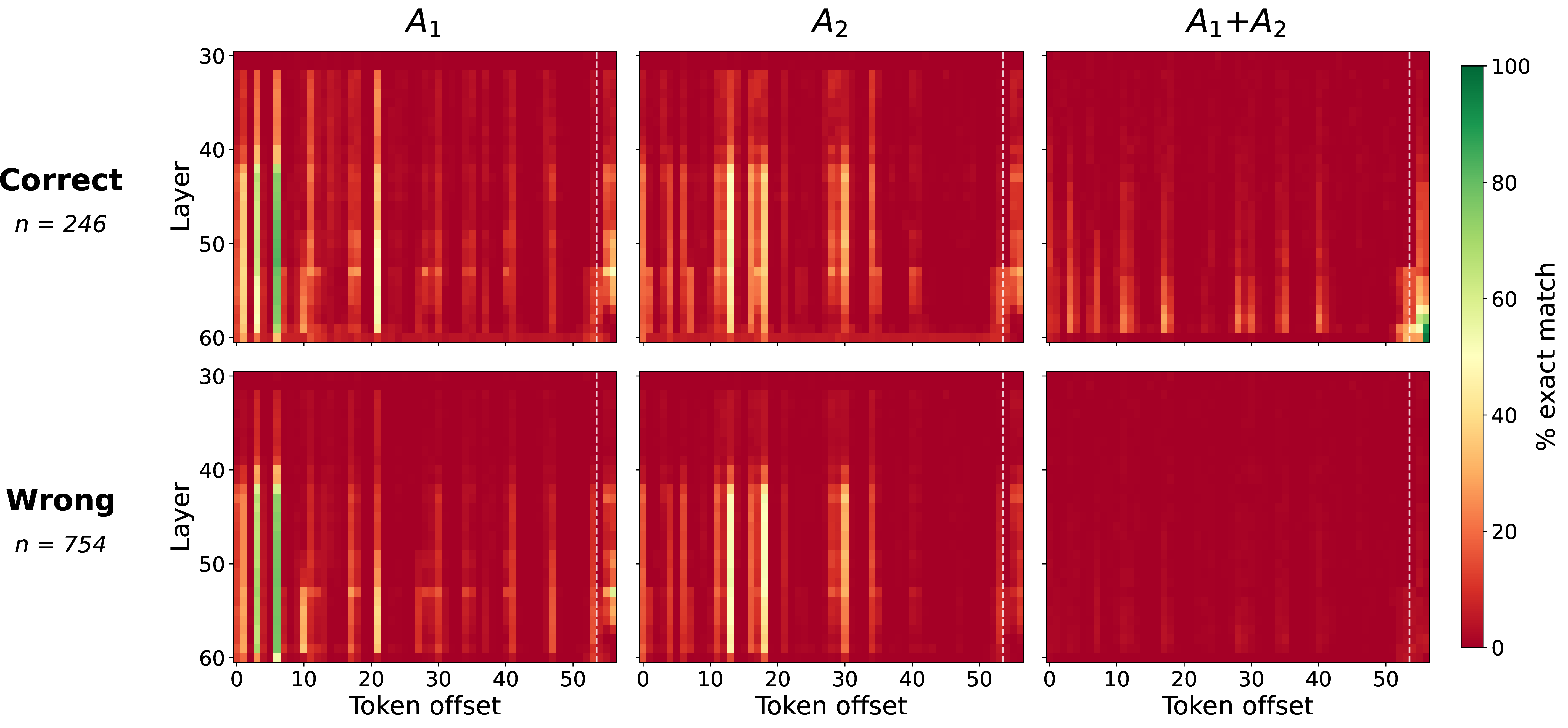
Figure 3 shows that, for 2-fact addition with DeepSeek V3 and dot-10 filler, the intermediate computation values \(A_1\) and \(A_2\) are encoded in filler token positions. We now show the baseline (no filler) for 2-fact addition (Figure 7). We also show that the same pattern of encoding extends to Kimi K2 (figure 8), counting filler (figure 9), and longer filler lengths (figure 10).
13 Position-resolved KV-cache transplants on 2-fact addition↩︎
The main-text transplants (Section 4) establish that filler content is causal for the answer on 1-fact addition and on the system of equations, in both cases by transplanting the entire filler region. This appendix reports the position-resolved 2-fact transplant, which tests the stronger claim that the positional structure of the encoding (\(A_1\) and \(A_2\) most strongly decoded at distinct filler positions, as seen in Appendix 12) is itself causal. All results are on DeepSeek V3 with \(k=50\) dot filler (53 filler positions), chosen so that each addend occupies enough distinct positions to transplant separately.
13.0.0.1 Position labeling.
Using the logit lens on correct examples, we label a filler position “\(A_1\)” if, at one or more layers, the top numeric token equals \(A_1\) in more than 15% of examples (threshold \(\theta = 0.15\)), and analogously for \(A_2\). At \(k=50\) this yields 12 \(A_1\)-decoded positions and 16 \(A_2\)-decoded positions. The two labels are independent: a position may pass both thresholds (for instance, a position decoding \(A_1\) in 50% and \(A_2\) in 35% of examples), in which case it appears in both decoded sets. This is allowed under fact-matching because in the \(A_1\) experiment the \(A_2\) content at such a position is held fixed across donor and target, so only its \(A_1\) content is effectively transplanted (and vice versa). We also ran \(\theta \in \{0.20, 0.30\}\); higher thresholds admit fewer positions and weaken the localization, consistent with each addend being distributed across several positions, so we report the most inclusive setting, \(\theta = 0.15\).
13.0.0.2 Fact-matched pairs.
To isolate one addend’s channel, we construct donor/target pairs that share the other addend. For the \(A_1\) channel, donor and target ask for \(A_1^{d}{+}A_2\) and \(A_1^{t}{+}A_2\) respectively; that is, the same second element \(A_2\), different first elements (\(A_1^{d} \neq A_1^{t}\)). Because atomic numbers are unique, the held-fixed addend never collides in value. Any shift in the target’s answer is then attributable to the varied addend alone, and the positions encoding the held-fixed addend carry near-identical content across the pair, making their transplant close to a no-op. We use 405 both-correct pairs for the \(A_1\) channel and 436 for the \(A_2\) channel, sampled as in the 1-fact protocol (Section 4).
13.0.0.3 Transplant scopes and metrics.
For each pair we transplant the donor’s KV cache, at the chosen positions, into the target’s forward pass, at three scopes: (i) whole, all 53 filler positions; (ii) the addend’s decoded positions (\(\theta=0.15\)); and (iii) the complement (all filler positions not labeled for that addend). We report two quantities, matching the main-text transplants: the rank shift, the improvement in the rank of the donor answer
\(A_1^{d}{+}A_2\) in the target’s next-token distribution relative to its unmodified baseline rank (positive = the donor answer became more likely); and the full-swap rate, the fraction of targets whose top output
token becomes the donor’s answer outright.
13.0.0.4 Results.
Table 1 reports all three scopes for both channels. The causal effect concentrates where the heatmap places the value. Transplanting only the decoded positions recovers 93% (\(A_1\)) and 85% (\(A_2\)) of the corresponding whole-filler rank shift, despite using only 12 and 16 of the 53 positions. The complementary positions—the majority of the filler region—move the rank by only 12 places and essentially never produce a full swap (0.0% for \(A_1\), 0.2% for \(A_2\)). (The decoded and complement contributions need not sum to the whole-filler shift, since the transplant is nonlinear in the number of positions perturbed.) Consistent with the system-of-equations result, two-operand transplants perturb the target’s computation more often than they cleanly replace it, resulting in few full-swaps. The \(A_1\) channel moves the answer somewhat more readily than \(A_2\) at every scope (whole-filler swap 7.4% vs.%), in line with \(A_1\) being the more strongly encoded addend. Each addend is independently and positionally manipulable, and the positions the lens reads as carrying neither addend carry essentially no causal load, so the positional layout is a causal feature of the computation rather than an artifact of the logit lens.
| Channel | Scope | # pos. | Rank shift | Full-swap (%) |
|---|---|---|---|---|
| \(A_1\) | all filler | 53 | 70 [61, 85] | 7.4 [4.9, 10.1] |
| (base rank 88) | \(A_1\)-decoded (\(\theta{=}0.15\)) | 12 | 65 [54, 76] | 4.4 [2.5, 6.7] |
| complement | 41 | 12 [9, 16] | 0.0 [0.0, 0.0] | |
| \(A_2\) | all filler | 53 | 58 [44, 73] | 2.8 [1.4, 4.4] |
| (base rank 90) | \(A_2\)-decoded (\(\theta{=}0.15\)) | 16 | 49 [38, 63] | 1.1 [0.2, 2.3] |
| complement | 37 | 12 [9, 16] | 0.2 [0.0, 0.7] |
14 LLM judge prompts↩︎
Neutral judge prompt
For 1-fact addition (asks for 1 number) and 2-fact addition (asks for 2 numbers):
For 2-hop letter position:
### system
These are potentially important tokens that were taken from a model’s internal state during a task. The tokens in this list are hints about what specific concept, entity, or name the model was ‘thinking about’ in its internal state while doing the
calculation, when it has not yet gotten to outputting the final answer. The original prompt contained formatting words like ‘Filler’ and ‘Answer’ that are not relevant to the task. The model was trained on Chinese data, so it may use Chinese tokens as well
as English.
What specific thing (person, place, object, concept, etc.) was the model thinking about?
Think briefly, then end your response with a JSON object on its own line:
{"answer": <string>, "confidence": <float 0-1>, "backups": [<string>, <string>, ... up to 10 ranked alternatives]}. If you cannot determine an answer, output null for that field.
### user
For the prompt sensitivity tests, the task-specific prompt is edited to name the expected target type: "What city was the model thinking about?" or "What chemical element was the model thinking about?"
15 Top-\(K\) token accuracy↩︎
For numeric intermediates (1-fact and 2-fact addition), we restrict to numeric tokens and check exact rank. For string-valued intermediates (element and city names in the letter-position task), we use a top-\(K\) substring coverage measure: each example has a multilingual reference dictionary containing the canonical English name, the chemical symbol where applicable, and a list of language aliases (English plus Chinese, since both models tokenize Chinese densely). A token at rank \(r\) is counted as a match if (i) it equals the chemical symbol exactly (case-sensitive, to avoid over-matching short English words), or (ii) it has a bidirectional case-insensitive substring overlap with any alias, with a minimum-length threshold of 4 characters for Latin-script tokens and 2 for CJK tokens. The bidirectional check captures both the case where the alias is a substring of the token and the case where the tokenizer splits the alias across multiple sub-tokens. Top-\(K\) accuracy is the fraction of examples for which any match fires at rank \(\leq K\). This baseline serves as a test of how much signal is in the aggregated tokens themselves versus how much is added by the judge.
16 Full decoding results (correct examples)↩︎
Tables 2–5 report the full top-\(K\) decoding results used to evaluate how much task-relevant information is recoverable from the model residual stream after filler-token generation. For each experimental group, we report the sample size \(n\) and the percentage of examples for which the correct target appears within the top-\(K\) decoded candidates, for \(K \in \{1,2,3,5,10\}\).
We include three decoding procedures. In the direct match setting, we aggregate residual-stream token scores and check whether the target appears among the top-\(K\) decoded tokens. For addition tasks, this is computed over the top-\(K\) numeric tokens. For letter-position tasks, this is computed over the top-\(K\) string tokens, allowing matches in either English or Chinese. In the Haiku and Sonnet judge settings, we instead ask a Claude model to infer the most likely latent target from the decoded candidates; top-\(K\) accuracy is computed by checking whether the target appears in the judge’s primary guess or first \(K{-}1\) backup guesses. The neutral judge prompt is task-agnostic, while the leading judge prompts provide the relevant domain framing, such as chemistry for element names or geography for capitals.
For the 1-fact addition task, the target is the single retrieved value \(A\). For the 2-fact addition task, a trial is counted as correct only when both addends, \(A_1\) and \(A_2\), are recovered within the top-\(K\) set. For the letter-position task, the target is the latent entity whose name supplies the requested letter. These appendix tables provide the full breakdown by filler type, filler length, model, and judge prompt, complementing the summary results in the main text.
Tables 6–7 provide shuffled-token baseline controls. In these controls, each example’s decoded top-50 token list is replaced with the top-50 list from a different example drawn from the same model, task, and filler condition, while the judge is still evaluated against the original example’s ground truth. If the judge were succeeding mainly by exploiting a task-level prior or the prompt framing, accuracy would remain high under this shuffle. The near-zero shuffled accuracy therefore shows that judge performance depends on information specific to the original example, not merely on generic task structure or prompt-induced guessing.
| Direct match top-\(K\) (%) | Haiku judge top-\(K\) (%) | Sonnet judge top-\(K\) (%) | ||||||||||||||
|---|---|---|---|---|---|---|---|---|---|---|---|---|---|---|---|---|
| 3-7 (lr)8-12 (lr)13-17 Group | \(n\) | 1 | 2 | 3 | 5 | 10 | 1 | 2 | 3 | 5 | 10 | 1 | 2 | 3 | 5 | 10 |
| dots_10 | 350 | 66.0 | 80.6 | 86.9 | 92.9 | 95.7 | 74.6 | 87.7 | 90.6 | 93.4 | 96.6 | 84.3 | 92.9 | 95.1 | 98.3 | 98.9 |
| dots_25 | 359 | 65.5 | 84.7 | 90.8 | 94.2 | 96.1 | 78.3 | 91.9 | 93.6 | 95.3 | 97.5 | 88.3 | 95.3 | 96.7 | 99.2 | 100.0 |
| dots_50 | 357 | 56.9 | 81.2 | 88.0 | 94.1 | 95.8 | 66.1 | 85.2 | 90.8 | 94.4 | 96.9 | 79.0 | 91.9 | 95.8 | 97.5 | 98.9 |
| dots_100 | 367 | 40.6 | 76.3 | 90.5 | 94.8 | 96.5 | 60.2 | 86.4 | 92.9 | 96.2 | 98.1 | 74.4 | 91.6 | 95.1 | 97.8 | 99.2 |
| counting_5 | 361 | 71.2 | 86.4 | 91.7 | 96.7 | 98.3 | 79.8 | 89.8 | 92.5 | 94.5 | 97.8 | 85.6 | 95.8 | 97.5 | 98.6 | 99.4 |
| counting_25 | 368 | 71.5 | 93.2 | 96.5 | 98.4 | 99.5 | 81.5 | 93.8 | 96.5 | 97.8 | 98.6 | 88.9 | 95.9 | 97.8 | 99.2 | 99.2 |
| counting_50 | 364 | 61.5 | 91.2 | 96.4 | 98.1 | 98.9 | 74.7 | 91.2 | 95.3 | 97.5 | 99.2 | 82.1 | 95.3 | 97.8 | 98.6 | 99.2 |
| alphabet_10 | 351 | 68.9 | 86.0 | 90.9 | 94.0 | 95.7 | 76.9 | 89.2 | 91.7 | 94.3 | 96.9 | 86.0 | 96.6 | 96.6 | 97.4 | 98.9 |
| alphabet_25 | 362 | 69.1 | 83.7 | 90.1 | 93.1 | 94.5 | 76.0 | 89.0 | 92.0 | 95.0 | 97.0 | 84.8 | 93.1 | 96.1 | 98.1 | 99.2 |
| Pooled | 3,239 | 63.4 | 84.8 | 91.3 | 95.2 | 96.8 | 74.2 | 89.3 | 92.9 | 95.4 | 97.6 | 83.7 | 94.3 | 96.5 | 98.3 | 99.2 |
2.2pt
| Direct match top-\(K\) (%) | Haiku judge top-\(K\) (%) | Sonnet judge top-\(K\) (%) | ||||||||||||||
|---|---|---|---|---|---|---|---|---|---|---|---|---|---|---|---|---|
| 3-7 (lr)8-12 (lr)13-17 Group | \(n\) | 1 | 2 | 3 | 5 | 10 | 1 | 2 | 3 | 5 | 10 | 1 | 2 | 3 | 5 | 10 |
| DeepSeek V3 | ||||||||||||||||
| dots_10 | 244 | 0.0 | 34.0 | 44.7 | 55.7 | 63.1 | 0.0 | 56.1 | 70.5 | 76.6 | 79.5 | 0.0 | 82.4 | 89.8 | 91.8 | 93.0 |
| dots_25 | 245 | 0.0 | 31.0 | 49.0 | 59.6 | 66.5 | 0.0 | 53.1 | 65.7 | 75.1 | 82.9 | 0.0 | 82.0 | 92.2 | 94.3 | 97.1 |
| dots_50 | 246 | 0.0 | 29.3 | 44.7 | 60.2 | 71.5 | 0.0 | 48.8 | 66.7 | 74.8 | 85.8 | 0.0 | 86.6 | 94.3 | 96.3 | 97.2 |
| counting_10 | 235 | 0.0 | 37.0 | 59.1 | 72.3 | 80.4 | 0.0 | 43.4 | 60.4 | 70.2 | 79.1 | 0.0 | 78.3 | 89.8 | 93.2 | 96.2 |
| counting_25 | 257 | 0.0 | 45.1 | 61.5 | 74.7 | 89.5 | 0.0 | 55.3 | 71.2 | 77.8 | 83.7 | 0.0 | 82.1 | 89.9 | 92.6 | 95.3 |
| counting_50 | 233 | 0.0 | 35.2 | 55.8 | 76.8 | 88.0 | 0.0 | 49.4 | 70.0 | 79.8 | 82.8 | 0.0 | 82.4 | 89.7 | 92.7 | 94.0 |
| DSv3 pooled | 1,460 | 0.0 | 35.3 | 52.5 | 66.5 | 76.5 | 0.0 | 51.1 | 67.5 | 75.8 | 82.3 | 0.0 | 82.3 | 91.0 | 93.5 | 95.5 |
| Kimi K2 | ||||||||||||||||
| dots_10 | 330 | 0.0 | 72.4 | 83.6 | 87.9 | 88.8 | 0.0 | 73.6 | 84.5 | 88.8 | 92.4 | 0.0 | 86.7 | 93.9 | 96.7 | 97.6 |
| dots_25 | 346 | 0.0 | 67.9 | 80.3 | 87.6 | 90.5 | 0.0 | 73.4 | 82.9 | 86.7 | 89.0 | 0.0 | 84.1 | 89.3 | 92.5 | 95.7 |
| dots_50 | 333 | 0.0 | 75.7 | 87.4 | 95.2 | 96.7 | 0.0 | 77.2 | 86.8 | 91.0 | 95.8 | 0.0 | 93.1 | 96.1 | 97.6 | 99.7 |
| counting_10 | 348 | 0.0 | 74.4 | 86.8 | 92.2 | 95.7 | 0.0 | 73.0 | 87.6 | 91.1 | 94.8 | 0.0 | 88.2 | 96.8 | 98.3 | 99.1 |
| counting_25 | 369 | 0.0 | 75.1 | 91.3 | 96.7 | 98.9 | 0.0 | 77.0 | 86.2 | 92.1 | 95.1 | 0.0 | 93.0 | 96.7 | 98.1 | 99.2 |
| counting_50 | 356 | 0.0 | 78.9 | 88.8 | 96.1 | 99.7 | 0.0 | 79.8 | 88.5 | 91.3 | 94.4 | 0.0 | 94.7 | 97.2 | 97.8 | 98.9 |
| KK2 pooled | 2,082 | 0.0 | 74.1 | 86.5 | 92.7 | 95.1 | 0.0 | 75.7 | 86.1 | 90.2 | 93.6 | 0.0 | 90.0 | 95.1 | 96.8 | 98.4 |
2.2pt
| Direct match top-\(K\) (%) | Haiku judge top-\(K\) (%) | Sonnet judge top-\(K\) (%) | ||||||||||||||
|---|---|---|---|---|---|---|---|---|---|---|---|---|---|---|---|---|
| 3-7 (lr)8-12 (lr)13-17 Group | \(n\) | 1 | 2 | 3 | 5 | 10 | 1 | 2 | 3 | 5 | 10 | 1 | 2 | 3 | 5 | 10 |
| DSv3, Elements | ||||||||||||||||
| dots_10 | 236 | 65.7 | 77.1 | 83.5 | 88.6 | 93.2 | 81.4 | 91.1 | 91.9 | 94.1 | 95.3 | 86.4 | 96.2 | 97.9 | 99.6 | 100.0 |
| dots_25 | 230 | 61.3 | 72.2 | 79.6 | 88.7 | 94.3 | 87.0 | 91.3 | 93.0 | 93.9 | 94.8 | 87.8 | 98.3 | 99.1 | 100.0 | 100.0 |
| dots_50 | 231 | 60.6 | 71.9 | 79.7 | 85.7 | 93.1 | 87.9 | 91.3 | 92.2 | 93.1 | 95.7 | 89.6 | 97.0 | 99.1 | 100.0 | 100.0 |
| counting_10 | 237 | 72.6 | 81.4 | 84.8 | 90.3 | 94.5 | 86.9 | 90.3 | 92.4 | 93.7 | 95.4 | 88.6 | 98.3 | 99.2 | 99.6 | 100.0 |
| counting_25 | 233 | 66.5 | 77.7 | 83.3 | 88.4 | 93.6 | 85.8 | 90.6 | 91.8 | 94.0 | 95.7 | 89.3 | 97.9 | 98.7 | 99.6 | 99.6 |
| counting_50 | 236 | 64.8 | 75.0 | 83.9 | 89.0 | 93.2 | 84.3 | 90.3 | 91.1 | 92.4 | 93.2 | 87.7 | 97.5 | 98.3 | 99.2 | 99.2 |
| DSv3, El pooled | 1,403 | 65.3 | 75.9 | 82.5 | 88.5 | 93.7 | 85.5 | 90.8 | 92.1 | 93.5 | 95.0 | 88.2 | 97.5 | 98.7 | 99.6 | 99.8 |
| DSv3, Capitals | ||||||||||||||||
| dots_10 | 218 | 45.4 | 58.3 | 61.9 | 70.6 | 78.4 | 64.2 | 78.9 | 82.1 | 84.4 | 84.9 | 69.3 | 86.2 | 88.1 | 90.4 | 90.8 |
| dots_25 | 216 | 44.9 | 57.9 | 61.6 | 67.6 | 76.9 | 69.4 | 81.5 | 82.9 | 85.2 | 85.6 | 70.8 | 88.0 | 89.4 | 90.7 | 91.2 |
| dots_50 | 216 | 46.8 | 53.2 | 62.5 | 69.4 | 76.4 | 67.6 | 77.8 | 81.5 | 84.7 | 85.2 | 73.6 | 86.1 | 88.4 | 90.7 | 92.1 |
| counting_10 | 214 | 47.2 | 55.6 | 60.7 | 68.2 | 75.7 | 73.8 | 84.1 | 86.9 | 90.2 | 90.7 | 79.0 | 87.4 | 87.4 | 90.7 | 90.7 |
| counting_25 | 218 | 46.3 | 58.7 | 61.9 | 69.7 | 76.6 | 69.7 | 79.8 | 82.1 | 84.9 | 86.2 | 76.1 | 87.2 | 88.1 | 90.4 | 90.8 |
| counting_50 | 217 | 47.0 | 62.2 | 65.4 | 69.1 | 76.0 | 71.4 | 81.1 | 83.4 | 85.3 | 86.2 | 77.9 | 90.8 | 91.2 | 92.6 | 94.0 |
| DSv3, Cap pooled | 1,299 | 46.3 | 57.7 | 62.4 | 69.1 | 76.7 | 69.4 | 80.5 | 83.1 | 85.8 | 86.5 | 74.4 | 87.6 | 88.8 | 90.9 | 91.6 |
| KK2, Elements | ||||||||||||||||
| dots_10 | 237 | 56.1 | 67.9 | 75.1 | 83.1 | 94.1 | 86.1 | 88.6 | 91.6 | 91.6 | 92.8 | 88.6 | 95.8 | 97.5 | 99.6 | 100.0 |
| dots_25 | 237 | 50.6 | 64.6 | 73.0 | 82.3 | 92.0 | 87.3 | 89.5 | 90.3 | 90.7 | 92.4 | 88.6 | 95.4 | 97.0 | 98.3 | 98.3 |
| dots_50 | 248 | 51.2 | 61.7 | 73.4 | 82.7 | 89.1 | 88.3 | 91.9 | 93.1 | 95.2 | 96.4 | 89.9 | 95.6 | 97.2 | 98.4 | 98.8 |
| counting_10 | 234 | 58.5 | 72.6 | 78.6 | 87.6 | 92.7 | 89.3 | 91.9 | 92.3 | 93.6 | 94.9 | 90.2 | 97.0 | 98.3 | 99.1 | 99.1 |
| counting_25 | 249 | 52.6 | 70.7 | 79.5 | 84.3 | 92.0 | 87.6 | 89.2 | 91.2 | 93.6 | 94.4 | 87.6 | 96.4 | 97.6 | 98.4 | 98.8 |
| counting_50 | 238 | 55.0 | 68.1 | 77.3 | 84.9 | 89.5 | 86.6 | 89.5 | 90.3 | 92.4 | 95.8 | 89.9 | 97.1 | 97.5 | 98.7 | 99.2 |
| KK2, El pooled | 1,443 | 54.0 | 67.6 | 76.2 | 84.1 | 91.5 | 87.5 | 90.1 | 91.5 | 92.9 | 94.5 | 89.1 | 96.2 | 97.5 | 98.8 | 99.0 |
| KK2, Capitals | ||||||||||||||||
| dots_10 | 261 | 46.0 | 57.5 | 60.5 | 65.1 | 70.5 | 63.6 | 74.3 | 77.4 | 80.8 | 82.4 | 62.1 | 78.9 | 82.8 | 85.4 | 85.8 |
| dots_25 | 259 | 45.6 | 56.8 | 61.4 | 65.6 | 70.7 | 61.0 | 77.6 | 79.5 | 80.7 | 81.5 | 62.9 | 84.2 | 85.7 | 87.3 | 88.0 |
| dots_50 | 258 | 46.5 | 54.7 | 61.6 | 65.1 | 70.2 | 66.3 | 77.9 | 80.6 | 81.8 | 82.2 | 68.6 | 84.9 | 85.7 | 87.6 | 88.0 |
| counting_10 | 254 | 46.5 | 61.0 | 63.8 | 69.7 | 72.8 | 59.8 | 76.4 | 78.3 | 81.1 | 81.5 | 66.1 | 84.3 | 86.6 | 87.8 | 87.8 |
| counting_25 | 259 | 47.5 | 59.5 | 64.5 | 66.8 | 69.5 | 67.6 | 81.5 | 82.6 | 84.9 | 85.3 | 71.8 | 87.3 | 89.2 | 91.1 | 91.5 |
| counting_50 | 263 | 47.9 | 60.8 | 63.1 | 66.2 | 70.7 | 70.7 | 81.4 | 83.7 | 84.8 | 85.6 | 78.3 | 87.8 | 89.0 | 90.1 | 90.9 |
| KK2, Cap pooled | 1,554 | 46.7 | 58.4 | 62.5 | 66.4 | 70.7 | 64.9 | 78.2 | 80.4 | 82.4 | 83.1 | 68.3 | 84.6 | 86.5 | 88.2 | 88.7 |
1.8pt
| Direct match top-\(K\) (%) | Haiku judge top-\(K\) (%) | Sonnet judge top-\(K\) (%) | ||||||||||||||
|---|---|---|---|---|---|---|---|---|---|---|---|---|---|---|---|---|
| 3-7 (lr)8-12 (lr)13-17 Group | \(n\) | 1 | 2 | 3 | 5 | 10 | 1 | 2 | 3 | 5 | 10 | 1 | 2 | 3 | 5 | 10 |
| DSv3, Elements | ||||||||||||||||
| dots_10 | 236 | 65.7 | 77.1 | 83.5 | 88.6 | 93.2 | 83.9 | 95.3 | 98.3 | 98.7 | 98.7 | 85.6 | 96.2 | 97.9 | 98.7 | 98.7 |
| dots_25 | 230 | 61.3 | 72.2 | 79.6 | 88.7 | 94.3 | 87.4 | 96.5 | 97.4 | 98.3 | 98.3 | 90.0 | 98.3 | 99.1 | 99.6 | 99.6 |
| dots_50 | 231 | 60.6 | 71.9 | 79.7 | 85.7 | 93.1 | 88.3 | 95.2 | 97.8 | 98.3 | 98.3 | 89.6 | 97.4 | 98.7 | 99.1 | 99.1 |
| counting_10 | 237 | 72.6 | 81.4 | 84.8 | 90.3 | 94.5 | 87.8 | 95.4 | 98.3 | 98.7 | 98.7 | 89.9 | 97.9 | 97.9 | 98.3 | 98.3 |
| counting_25 | 233 | 66.5 | 77.7 | 83.3 | 88.4 | 93.6 | 87.1 | 96.6 | 98.3 | 99.1 | 99.1 | 89.7 | 97.4 | 98.3 | 98.7 | 98.7 |
| counting_50 | 236 | 64.8 | 75.0 | 83.9 | 89.0 | 93.2 | 85.2 | 94.9 | 97.0 | 97.9 | 97.9 | 89.4 | 97.9 | 98.7 | 98.7 | 98.7 |
| DSv3, El pooled | 1,403 | 65.3 | 75.9 | 82.5 | 88.5 | 93.7 | 86.6 | 95.7 | 97.9 | 98.5 | 98.5 | 89.0 | 97.5 | 98.4 | 98.9 | 98.9 |
| DSv3, Capitals | ||||||||||||||||
| dots_10 | 218 | 45.4 | 58.3 | 61.9 | 70.6 | 78.4 | 83.5 | 89.4 | 90.4 | 91.7 | 91.7 | 87.6 | 92.7 | 93.1 | 94.0 | 95.0 |
| dots_25 | 216 | 44.9 | 57.9 | 61.6 | 67.6 | 76.9 | 84.3 | 88.9 | 90.7 | 91.2 | 91.2 | 88.0 | 94.0 | 94.9 | 95.8 | 95.8 |
| dots_50 | 216 | 46.8 | 53.2 | 62.5 | 69.4 | 76.4 | 85.2 | 89.4 | 90.7 | 91.7 | 91.7 | 88.9 | 91.7 | 92.6 | 93.5 | 94.4 |
| counting_10 | 214 | 47.2 | 55.6 | 60.7 | 68.2 | 75.7 | 86.0 | 91.1 | 92.1 | 93.0 | 93.0 | 89.7 | 92.5 | 93.9 | 94.4 | 94.4 |
| counting_25 | 218 | 46.3 | 58.7 | 61.9 | 69.7 | 76.6 | 84.9 | 89.0 | 90.4 | 90.8 | 90.8 | 86.7 | 92.2 | 93.1 | 94.0 | 94.0 |
| counting_50 | 217 | 47.0 | 62.2 | 65.4 | 69.1 | 76.0 | 86.2 | 89.9 | 91.2 | 92.2 | 92.2 | 90.3 | 94.5 | 95.9 | 96.3 | 96.3 |
| DSv3, Cap pooled | 1,299 | 46.3 | 57.7 | 62.4 | 69.1 | 76.7 | 85.0 | 89.6 | 90.9 | 91.8 | 91.8 | 88.5 | 92.9 | 93.9 | 94.7 | 95.0 |
| KK2, Elements | ||||||||||||||||
| dots_10 | 237 | 56.1 | 67.9 | 75.1 | 83.1 | 94.1 | 87.3 | 93.7 | 97.0 | 97.5 | 97.9 | 88.6 | 96.6 | 99.2 | 99.2 | 99.6 |
| dots_25 | 237 | 50.6 | 64.6 | 73.0 | 82.3 | 92.0 | 88.6 | 93.7 | 95.4 | 97.0 | 97.0 | 86.9 | 95.8 | 97.9 | 98.7 | 98.7 |
| dots_50 | 248 | 51.2 | 61.7 | 73.4 | 82.7 | 89.1 | 86.7 | 93.1 | 96.4 | 97.6 | 97.6 | 87.5 | 95.6 | 98.0 | 98.4 | 98.4 |
| counting_10 | 234 | 58.5 | 72.6 | 78.6 | 87.6 | 92.7 | 89.7 | 96.2 | 97.4 | 98.7 | 98.7 | 89.7 | 97.0 | 98.3 | 98.7 | 98.7 |
| counting_25 | 249 | 52.6 | 70.7 | 79.5 | 84.3 | 92.0 | 88.0 | 96.0 | 98.4 | 99.6 | 99.6 | 88.0 | 96.4 | 98.4 | 98.4 | 98.8 |
| counting_50 | 238 | 55.0 | 68.1 | 77.3 | 84.9 | 89.5 | 90.3 | 96.6 | 98.3 | 98.7 | 98.7 | 89.5 | 97.1 | 98.7 | 99.6 | 99.6 |
| KK2, El pooled | 1,443 | 54.0 | 67.6 | 76.2 | 84.1 | 91.5 | 88.4 | 94.9 | 97.2 | 98.2 | 98.3 | 88.4 | 96.4 | 98.4 | 98.8 | 99.0 |
| KK2, Capitals | ||||||||||||||||
| dots_10 | 261 | 46.0 | 57.5 | 60.5 | 65.1 | 70.5 | 77.0 | 87.7 | 89.3 | 89.3 | 89.3 | 84.3 | 90.0 | 91.2 | 92.3 | 92.7 |
| dots_25 | 259 | 45.6 | 56.8 | 61.4 | 65.6 | 70.7 | 79.2 | 87.3 | 88.8 | 89.6 | 89.6 | 84.6 | 89.6 | 90.3 | 92.7 | 93.1 |
| dots_50 | 258 | 46.5 | 54.7 | 61.6 | 65.1 | 70.2 | 79.1 | 87.6 | 88.0 | 88.0 | 88.0 | 83.3 | 90.3 | 93.0 | 93.0 | 93.4 |
| counting_10 | 254 | 46.5 | 61.0 | 63.8 | 69.7 | 72.8 | 79.1 | 85.0 | 86.6 | 89.4 | 89.4 | 85.4 | 90.2 | 91.7 | 92.1 | 92.1 |
| counting_25 | 259 | 47.5 | 59.5 | 64.5 | 66.8 | 69.5 | 79.2 | 86.9 | 88.8 | 89.6 | 89.6 | 86.9 | 91.1 | 91.9 | 93.1 | 94.2 |
| counting_50 | 263 | 47.9 | 60.8 | 63.1 | 66.2 | 70.7 | 79.5 | 87.8 | 88.6 | 89.7 | 89.7 | 86.7 | 92.0 | 92.8 | 93.5 | 93.5 |
| KK2, Cap pooled | 1,554 | 46.7 | 58.4 | 62.5 | 66.4 | 70.7 | 78.8 | 87.1 | 88.4 | 89.3 | 89.3 | 85.2 | 90.5 | 91.8 | 92.8 | 93.2 |
1.8pt
| Task | Judge | Prompt | Method | \(n\) | 1 | 2 | 3 | 5 | 10 |
|---|---|---|---|---|---|---|---|---|---|
| 1-fact | Haiku | neutral | orig. | 350 | 74.6 | 87.7 | 90.6 | 93.4 | 96.6 |
| shuf. | 350 | 0.6 | 1.4 | 2.0 | 3.1 | 4.3 | |||
| \(\Delta\) | -74.0 | -86.3 | -88.6 | -90.3 | -92.3 | ||||
| -fact | Sonnet | neutral | orig. | 350 | 84.3 | 92.9 | 95.1 | 98.3 | 98.9 |
| shuf. | 350 | 0.6 | 1.1 | 2.0 | 2.9 | 4.9 | |||
| \(\Delta\) | -83.7 | -91.7 | -93.1 | -95.4 | -94.0 | ||||
| -fact | Haiku | neutral | orig. | 244 | – | 56.1 | 70.5 | 76.6 | 79.5 |
| shuf. | 244 | – | 0.0 | 0.0 | 0.0 | 0.0 | |||
| \(\Delta\) | – | -56.1 | -70.5 | -76.6 | -79.5 | ||||
| -fact | Sonnet | neutral | orig. | 244 | – | 82.4 | 89.8 | 91.8 | 93.0 |
| shuf. | 244 | – | 0.0 | 0.0 | 0.0 | 0.4 | |||
| \(\Delta\) | – | -82.4 | -89.8 | -91.8 | -92.6 | ||||
| Letter-pos. | Haiku | neutral | orig. | 236 | 81.4 | 91.1 | 91.9 | 94.1 | 95.3 |
| shuf. | 236 | 0.4 | 0.8 | 0.8 | 1.3 | 1.3 | |||
| \(\Delta\) | -80.9 | -90.3 | -91.1 | -92.8 | -94.1 | ||||
| Letter-pos. | Sonnet | neutral | orig. | 236 | 86.4 | 96.2 | 97.9 | 99.6 | 100.0 |
| shuf. | 236 | 0.4 | 1.3 | 1.3 | 1.3 | 1.3 | |||
| \(\Delta\) | -86.0 | -94.9 | -96.6 | -98.3 | -98.7 | ||||
| Letter-pos. | Haiku | chem. | orig. | 236 | 83.9 | 95.3 | 98.3 | 98.7 | 98.7 |
| shuf. | 236 | 0.4 | 0.8 | 2.1 | 2.5 | 2.5 | |||
| \(\Delta\) | -83.5 | -94.5 | -96.2 | -96.2 | -96.2 | ||||
| Letter-pos. | Sonnet | chem. | orig. | 236 | 85.6 | 96.2 | 97.9 | 98.7 | 98.7 |
| shuf. | 236 | 0.4 | 1.3 | 2.5 | 2.5 | 2.5 | |||
| \(\Delta\) | -85.2 | -94.9 | -95.3 | -96.2 | -96.2 | ||||
| Capital-pos. | Haiku | neutral | orig. | 218 | 64.2 | 78.9 | 82.1 | 84.4 | 84.9 |
| shuf. | 218 | 0.5 | 0.5 | 0.5 | 0.5 | 0.5 | |||
| \(\Delta\) | -63.8 | -78.4 | -81.7 | -83.9 | -84.4 | ||||
| Capital-pos. | Sonnet | neutral | orig. | 218 | 69.3 | 86.2 | 88.1 | 90.4 | 90.8 |
| shuf. | 218 | 0.5 | 0.5 | 0.5 | 0.5 | 0.5 | |||
| \(\Delta\) | -68.8 | -85.8 | -87.6 | -89.9 | -90.4 | ||||
| Capital-pos. | Haiku | geo. | orig. | 218 | 83.5 | 89.4 | 90.4 | 91.7 | 91.7 |
| shuf. | 218 | 0.0 | 0.0 | 0.5 | 0.5 | 0.5 | |||
| \(\Delta\) | -83.5 | -89.4 | -89.9 | -91.3 | -91.3 | ||||
| Capital-pos. | Sonnet | geo. | orig. | 218 | 87.6 | 92.7 | 93.1 | 94.0 | 95.0 |
| shuf. | 218 | 0.0 | 0.0 | 0.5 | 0.9 | 0.9 | |||
| \(\Delta\) | -87.6 | -92.7 | -92.7 | -93.1 | -94.0 |
2.2pt
| Task | Judge | Prompt | Method | \(n\) | 1 | 2 | 3 | 5 | 10 |
|---|---|---|---|---|---|---|---|---|---|
| 2-fact | Haiku | neutral | orig. | 330 | – | 73.6 | 84.5 | 88.8 | 92.4 |
| shuf. | 330 | – | 0.3 | 0.3 | 0.3 | 0.6 | |||
| \(\Delta\) | – | -73.3 | -84.2 | -88.5 | -91.8 | ||||
| -fact | Sonnet | neutral | orig. | 330 | – | 86.7 | 93.9 | 96.7 | 97.6 |
| shuf. | 330 | – | 0.0 | 0.3 | 0.3 | 0.6 | |||
| \(\Delta\) | – | -86.7 | -93.6 | -96.4 | -97.0 | ||||
| Letter-pos. | Haiku | neutral | orig. | 237 | 86.1 | 88.6 | 91.6 | 91.6 | 92.8 |
| shuf. | 237 | 0.8 | 0.8 | 0.8 | 1.3 | 1.7 | |||
| \(\Delta\) | -85.2 | -87.8 | -90.7 | -90.3 | -91.1 | ||||
| Letter-pos. | Sonnet | neutral | orig. | 237 | 88.6 | 95.8 | 97.5 | 99.6 | 100.0 |
| shuf. | 237 | 1.3 | 1.3 | 2.5 | 3.8 | 3.8 | |||
| \(\Delta\) | -87.3 | -94.5 | -94.9 | -95.8 | -96.2 | ||||
| Letter-pos. | Haiku | chem. | orig. | 237 | 87.3 | 93.7 | 97.0 | 97.5 | 97.9 |
| shuf. | 237 | 1.3 | 1.7 | 3.0 | 4.2 | 4.2 | |||
| \(\Delta\) | -86.1 | -92.0 | -94.1 | -93.2 | -93.7 | ||||
| Letter-pos. | Sonnet | chem. | orig. | 237 | 88.6 | 96.6 | 99.2 | 99.2 | 99.6 |
| shuf. | 237 | 1.3 | 3.4 | 3.8 | 5.5 | 5.5 | |||
| \(\Delta\) | -87.3 | -93.2 | -95.4 | -93.7 | -94.1 | ||||
| Capital-pos. | Haiku | neutral | orig. | 261 | 63.6 | 74.3 | 77.4 | 80.8 | 82.4 |
| shuf. | 261 | 0.0 | 0.0 | 0.4 | 0.4 | 0.4 | |||
| \(\Delta\) | -63.6 | -74.3 | -77.0 | -80.5 | -82.0 | ||||
| Capital-pos. | Sonnet | neutral | orig. | 261 | 62.1 | 78.9 | 82.8 | 85.4 | 85.8 |
| shuf. | 261 | 0.4 | 0.4 | 0.4 | 0.4 | 0.4 | |||
| \(\Delta\) | -61.7 | -78.5 | -82.4 | -85.1 | -85.4 | ||||
| Capital-pos. | Haiku | geo. | orig. | 261 | 77.0 | 87.7 | 89.3 | 89.3 | 89.3 |
| shuf. | 261 | 0.4 | 0.8 | 0.8 | 0.8 | 0.8 | |||
| \(\Delta\) | -76.6 | -87.0 | -88.5 | -88.5 | -88.5 | ||||
| Capital-pos. | Sonnet | geo. | orig. | 261 | 84.3 | 90.0 | 91.2 | 92.3 | 92.7 |
| shuf. | 261 | 0.4 | 0.8 | 0.8 | 1.1 | 1.5 | |||
| \(\Delta\) | -83.9 | -89.3 | -90.4 | -91.2 | -91.2 |
2.2pt
17 System of equations: decoding results↩︎
This appendix gives the full decoding breakdown for the system-of-equations task on DeepSeek V3, pooled across six filler conditions (dot filler with \(k=10,25,50\) and counting filler with \(k=5,10,25\); \(n=1{,}824\)). Table 8 reports per-intermediate recovery at each top-\(K\); Table 9 reports the shuffled-token control alongside the (near-identical) judge performance; Table 10 reports where the decode lands when the queried variable \(y\) is not the top-1 token.
The intermediate value \(y\) is recovered nearly always (top-5 \(94.8\%\)), while the input \(x\), although given in the prompt, is barely present in the filler residual (top-5 \(21.9\%\)), and the two transient sub-products fall in between, with the later \(c_2 y\) more strongly encoded than the earlier \(c_1 x\). At top-5 the ordering is \(y\) (\(94.8\)) \(>\) \(c_2 y\) (\(85.6\)) \(>\) answer (\(65.0\)) \(>\) \(c_1 x\) (\(41.8\)) \(>\) \(x\) (\(21.9\)). Because the prompt carries no informative context, the Haiku and Sonnet judges track direct token recovery to within \(\sim1\) pp on every intermediate, in contrast to the retrieval tasks, where the judge adds up to tens of points.
| Target | top-1 | top-2 | top-3 | top-5 | top-10 |
|---|---|---|---|---|---|
| \(c_1 x\) | 3 | 11 | 22 | 42 | 64 |
| \(y\) | 55 | 82 | 89 | 95 | 97 |
| \(c_2 y\) | 30 | 61 | 75 | 86 | 93 |
| \(x\) (given) | 0 | 2 | 7 | 22 | 51 |
| answer | 6 | 22 | 44 | 65 | 80 |
8pt
| Target | Real (direct / Haiku / Sonnet) | Shuffled (direct / Haiku / Sonnet) |
|---|---|---|
| \(c_1 x\) | 41.8 / 42.9 / 42.3 | 1.7 / 2.0 / 2.0 |
| \(y\) | 94.8 / 95.3 / 95.6 | 1.3 / 1.7 / 1.6 |
| \(c_2 y\) | 85.6 / 85.7 / 85.9 | 0.5 / 1.0 / 1.0 |
| \(x\) | 21.9 / 22.0 / 22.0 | 1.3 / 2.0 / 2.0 |
| answer | 65.0 / 63.3 / 64.3 | 0.6 / 0.8 / 0.8 |
8pt
| Top-1 identity (when not \(y\)) | Share |
|---|---|
| \(c_2 y\) (next value in the chain) | 67% |
| answer | 14% |
| other problem quantity | 7% |
| \(c_1 x\) | 7% |
| off-problem | 5% |
| \(x\) (base) | 0% |
8pt
18 Full decoding results (incorrect examples)↩︎
Tables 11 and 12 extend the decoding analysis to incorrect examples on the dots-10 filler condition. The decoder runs identically on correct and incorrect examples; only the scoring requires correct examples to define the target. Direct top-2 token match, the most stringent measure of what surfaces in the residual stream, stays within \(\pm 10\) pp of correct-example accuracy on 5 of 7 (model, task) combinations, with the exceptions being 2-fact addition (where incorrect examples score higher) and capital-position (where they score lower). On 2-fact addition, both operands are in fact more recoverable on incorrect examples (DeepSeek V3: 34% \(\to\) 55%; Kimi K2: 72% \(\to\) 82% top-2 direct), because the sum \(A_1+A_2\) is essentially absent from the residual stream when the model fails, surfacing in the top-2 numeric tokens 10–16\(\times\) more often on correct examples than incorrect ones (Table 12). With no sum competing for top-\(K\) slots, the operands occupy them more readily. Both models exhibit the same asymmetry, suggesting “operands retrieved, sum not formed” is a property of the task structure rather than a quirk of either model. The exception is capital-position, where intermediate recovery does drop on incorrect examples (DeepSeek V3: \(-10\) pp direct; Kimi K2: \(-16\) pp), indicating that for some capital lookups the failure mode is missing retrieval rather than missing composition. Together, these results show that the decoder is diagnostic about where a computation fails. When retrieval succeeds but composition does not (2-fact), the operands surface clearly and the sum is missing; when retrieval itself fails (some capital-pos cases), the relevant intermediate is genuinely not in the residual stream to be decoded.
| Task | Subset | \(n\) | Direct (%) | Haiku (%) | Sonnet (%) |
|---|---|---|---|---|---|
| DeepSeek V3 | |||||
| 1-fact addition | correct | 350 | 80.6 | 87.7 | 92.9 |
| 1-fact addition | incorrect | 150 | 72.0 | 78.7 | 86.0 |
| 2-fact addition | correct | 244 | 34.0 | 56.1 | 82.4 |
| 2-fact addition | incorrect | 756 | 55.4 | 69.6 | 83.6 |
| Element-position | correct | 236 | 77.1 | 91.1 | 96.2 |
| Element-position | incorrect | 49 | 83.7 | 95.9 | 95.9 |
| Capital-position | correct | 218 | 58.3 | 78.9 | 86.2 |
| Capital-position | incorrect | 144 | 47.9 | 64.6 | 80.6 |
| Kimi K2 | |||||
| 2-fact addition | correct | 330 | 72.4 | 73.6 | 86.7 |
| 2-fact addition | incorrect | 670 | 81.8 | 83.4 | 88.8 |
| Element-position | correct | 237 | 67.9 | 88.6 | 95.8 |
| Element-position | incorrect | 48 | 64.6 | 93.8 | 97.9 |
| Capital-position | correct | 261 | 57.5 | 74.3 | 78.9 |
| Capital-position | incorrect | 101 | 41.6 | 53.5 | 67.3 |
| Model | Subset | \(n\) | Top-1 (%) | Top-2 (%) | Top-3 (%) | Top-5 (%) | Top-10 (%) |
|---|---|---|---|---|---|---|---|
| DeepSeek V3 | correct | 244 | 5.3 | 21.7 | 34.4 | 44.3 | 54.1 |
| DeepSeek V3 | incorrect | 756 | 0.3 | 2.0 | 4.0 | 7.3 | 15.3 |
| Kimi K2 | correct | 330 | 0.0 | 11.2 | 27.6 | 38.5 | 46.4 |
| Kimi K2 | incorrect | 670 | 0.0 | 0.7 | 4.0 | 9.3 | 14.0 |
19 Residual-subtraction ablation↩︎
Table 13 ablates the residual-subtraction step used in the main decoding pipeline. In the residualized setting, token scores are computed by subtracting the cross-example mean score for each layer–position setting; in the no-residual ablation, tokens are ranked directly by their raw logit-lens probabilities. This comparison isolates when residualization helps remove common filler or formatting artifacts, and when it can instead suppress useful signal.
Residualization can be significantly beneficial, but not always. On DeepSeek V3 2-fact addition with dots_10 filler, residualization improves Sonnet top-2 accuracy from 73.8% to 82.4%. However, with counting_10 filler, residualization reduces Haiku top-10 accuracy from 90.6% to 79.1%. Inspecting the decoded tokens suggests this occurs because counting filler makes digit tokens part of the cross-example baseline, and those same numeric tokens can be relevant to the target intermediates.
| Task | Cond. | Judge | Method | \(n\) | 1 | 2 | 3 | 5 | 10 |
|---|---|---|---|---|---|---|---|---|---|
| 2-fact | dots_10 | Haiku | residual | 244 | – | 56.1 | 70.5 | 76.6 | 79.5 |
| no-resid | 244 | – | 55.3 | 73.0 | 77.5 | 81.6 | |||
| -fact | dots_10 | Sonnet | residual | 244 | – | 82.4 | 89.8 | 91.8 | 93.0 |
| no-resid | 244 | – | 73.8 | 85.2 | 88.1 | 90.2 | |||
| -fact | counting_10 | Haiku | residual | 235 | – | 43.4 | 60.4 | 70.2 | 79.1 |
| no-resid | 235 | – | 45.1 | 67.2 | 79.6 | 90.6 | |||
| -fact | counting_10 | Sonnet | residual | 235 | – | 78.3 | 89.8 | 93.2 | 96.2 |
| no-resid | 235 | – | 68.1 | 83.0 | 88.9 | 94.0 | |||
| Letter-pos. | dots_10 | Haiku | residual | 454 | 73.1 | 85.2 | 87.2 | 89.4 | 90.3 |
| no-resid | 454 | 75.1 | 82.0 | 84.6 | 86.6 | 88.5 | |||
| Letter-pos. | dots_10 | Sonnet | residual | 454 | 78.2 | 91.4 | 93.2 | 95.2 | 95.6 |
| no-resid | 454 | 83.9 | 92.0 | 93.0 | 95.2 | 96.1 |
3.0pt