Amortising Bayesian Experimental Design for Sequential Information Gathering in LLMs
July 03, 2026
Abstract
Large language models (LLMs) exhibit strong reasoning and world-knowledge capabilities, yet often struggle to gather information effectively across the multi-turn interactions required in sequential decision-making settings. We introduce Amortised Sequential Information Gathering (ASIG), a fine-tuning approach that amortises Bayesian Experimental Design (BED) into LLM policies via a multi-turn extension of Group Relative Policy Optimisation with an Expected Information Gain reward. Evaluated on the 20 Questions task, ASIG more than doubles the success rate of the 7B base model and reduces inference cost by over \(25\times\) relative to BED-LLM, a competitive inference-time baseline. Applied to MediQ, a medical diagnosis benchmark unseen during training, ASIG improves information-seeking performance at the 7B scale, suggesting that the learned strategies can transfer out of distribution. Our findings show that amortising BED into LLM policies provides an effective and computationally efficient approach to sequential information gathering.
1 Introduction↩︎
Effective information gathering in sequential settings is fundamental to applications ranging from healthcare to designing experiments in scientific domains. LLMs are increasingly being deployed in such domains, as they are high capacity models encoding extensive world knowledge [1], and have shown promise in reasoning and decision-making tasks on diverse action spaces expressed in natural language [2]. However, despite these capabilities, LLMs have been shown to struggle with multi-turn reasoning and planning in various settings. One example is the “lost in conversation" phenomenon reported by [3], which demonstrates that LLMs often struggle to (1) recognize when additional information is needed to complete a task and (2) effectively acquire that information during multi-turn conversations. These limitations are particularly problematic for experimental design and sequential decision making, where maintaining and updating coherent beliefs over extended interactions is key.
A growing body of work has explored methods for improving the decision-making and information-gathering capabilities of LLMs in sequential settings. Broadly, there are two main classes of approaches: weight-space optimisation methods [4]–[8], which fine-tune the model parameters, and inference-time optimisation methods [9]–[11], which add post-processing procedures during inference. While demonstrating strong improvement in the information-gathering performance of LLMs in sequential settings, inference-time optimisation methods suffer from high computational cost during inference and must be tailored to a specific task or environment. On the other hand, weight-space optimisation methods yield fast inference time behaviour, but it remains to be seen whether these approaches improve general information gathering capabilities or just fit to the task at hand.
In this work, we introduce Amortised Sequential Information Gathering (ASIG), a weight-space optimisation framework that amortises Bayesian Experimental Design (BED) [12] into the weights of an LLM, enabling sequential information gathering without additional inference-time optimisation. We treat the LLM as a BED agent in a general sequential setting, where it iteratively selects experiments to maximally reduce uncertainty over a latent target. We then fine-tune the model using Expected Information Gain (EIG) as the reward signal within a multi-turn variant of Group Relative Policy Optimisation (GRPO) [13]. The reward combines EIG, which incentivises experiments that maximally reduce uncertainty over candidate targets, with an outcome-based signal that directly reinforces task success, trained via a learning curriculum across multi-turn rollouts. As a controlled instantiation of this framework, we train on the 20 Questions game, where binary outcomes make EIG tractable via a Rao-Blackwellised estimator and the capability being trained (asking maximally informative questions) is inherently domain-agnostic. We evaluate on held-out 20 Questions categories and assess generalisation to MediQ [14], exploring whether amortised BED behaviour transfers to real-world sequential information-gathering settings.
We summarise our contributions as follows:
We introduce ASIG, a novel fine-tuning method to amortise BED information gathering into LLMs.
We extend GRPO to support multiple reward streams with distinct temporal horizons, enabling joint optimisation of turn-level EIG and multi-horizon task success.
We demonstrate that ASIG substantially improves 20 Questions performance over the base model, more than doubling the success rate in the 7B model class, while outperforming a competitive inference-time baseline in two out of four settings at over 25× lower inference cost.
We show that the information-seeking behaviour learned by ASIG transfers to MediQ, a medical diagnosis benchmark, at the 7B scale without any in-domain fine-tuning.
2 Related Work↩︎
2.1 Inference-Time Optimisation Methods↩︎
Inference-time optimisation methods improve sequential decision making and question asking in LLMs by optimising information gathering directly at test time, without modifying model weights. In this setting, LLMs are treated as decision making agents in a sequential problem with a hidden target, where the next action is selected by explicitly maximizing EIG (or an EIG proxy) given the interaction history. BED-LLM [9] adopts this approach on the 20 Questions task. They use the LLM to propose candidate questions, define a uniform prior over the set of possible targets, and use the questions and possible targets to estimate EIG, eventually selecting the question with the highest score at each turn. Related methods adopt similar formulations, using sampling based EIG estimation for task disambiguation [10], or maintaining explicit Bayesian belief states with Monte Carlo estimation of the EIG [11].
These approaches consistently outperform naive prompting, offering principled uncertainty handling and interpretability through explicit belief updates, while remaining applicable to off-the-shelf LLMs. However, they incur substantial inference time cost due to sampling and belief maintenance, often rely on structured hypothesis spaces or simulators (e.g. 20 Questions-type tasks), and are typically myopic and task-specific which limits their actual usability.
2.2 Weight-Space Optimisation Methods↩︎
Weight-space methods for improving LLM information-gathering divide broadly into retriever-coupled and self-contained approaches. [6] and [7] both couple the LLM to an external retriever network that carries the belief state, deriving EIG or rank-based rewards from the retriever’s candidate distribution. However, neither evaluates transfer beyond their training tasks, and both are restricted to settings where retrieval infrastructure exists.
Self-contained approaches remove this dependency. [4] demonstrate that EIG is an effective training signal via Direct Preference Optimisation (DPO) [15] on a static dataset of EIG-ranked question pairs, but the fixed preference dataset cannot adapt to the model’s evolving question distribution, and generalisation is evaluated only within 20 Questions categories. [5] takes a complementary approach, using Relative Preference Optimisation (RPO) [16] on purely outcome-based rewards with no information-theoretic component. They demonstrate zero-shot transfer across a family of simple decision-making tasks, though the authors themselves note that online RL would likely yield stronger results than their offline preference optimisation.
\(\Delta\)Belief-RL [8] is the closest antecedent to our work: an online RL method that uses the change in the model’s assigned probability to the correct target as a dense per-turn reward, without any external retriever, and demonstrates OOD generalisation to customer service and personalisation settings. Our approach shares the same self-contained online RL paradigm, but uses EIG instead of \(\Delta\text{Belief(target)}\) as the reward signal. This distinction matters because EIG captures both the uncertainty of the marginal answer distribution and the sharpness of per-belief likelihoods, rather than tracking a single scalar probability whose change may not reflect genuine information gain.
3 Preliminary↩︎
3.1 Bayesian Experimental Design↩︎
BED provides a principled framework for experimental design grounded in Bayesian decision theory, in which experiments are selected based on their expected utility under an explicit probabilistic model of the world [12]. In the BED formulation, the uncertainty about a quantity of interest \(\theta\) is represented by a prior distribution \(p(\theta)\), while a likelihood model \(p(y |\theta, \xi)\) specifies how experimental outcomes \(y\) are generated under a proposed design \(\xi\). Together, these components define a joint probabilistic model over latent variables and observations, enabling candidate experiments to be evaluated prior to data collection by computing their expected utility. This explicit generative modelling distinguishes BED from heuristic or purely discriminative approaches to experimental design, and allows prior knowledge, measurement noise, and experimental constraints to be incorporated in a coherent Bayesian manner [17].
![Figure 2: Overview of our step-by-step EIG calculation, following the approach of BED-LLM [9]. 1) Plausible target entities (\theta) are sampled from the current belief state. 2) For each design (\xi_t), observation likelihoods p(y \mid \theta, \xi_t) are computed across all sampled targets. 3) These likelihoods are used to calculate the predictive entropy H(y_t \mid \xi_t) and expected conditional entropy \mathbb{E}[H(y_t|\theta,\xi_t)]. High-EIG designs are those that produce uncertain marginal observations (splitting the belief space) while minimizing conditional entropy.](/article/2607.03426/figures/eig.png "fig:")
3.1.0.1 Expected Information Gain.
First proposed by [18], EIG is a widely used optimality metric within BED. Given a latent variable \(\theta\), which we seek to learn about through an experiment \(\xi\), we define the Information Gain (IG) on \(\theta\) from an experimental outcome \(y\) by the reduction in Shannon entropy [19] from the prior to the posterior:
\[\operatorname{IG}_{\theta}(\xi) = H[p(\theta)] - H[p(\theta|y,\xi)].\] EIG is then calculated as the expectation of this quantity over the marginal predictive distribution, \(p(y|\xi)\): \[\begin{align} \operatorname{EIG}_{\theta}(\xi) &= \mathbb{E}_{p(y|\xi)}[\operatorname{IG}_{\theta}(\xi,y)] \label{eq:2} \\ &= \mathbb{E}_{p(\theta)p(y|\theta,\xi)}[\log{p(\theta|y,\xi)}-\log{p(\theta)}]\notag \\ &= \mathbb{E}_{p(\theta)p(y|\theta, \xi)}[\log{p(y|\theta,\xi)}-\log{p(y|\xi)}].\notag \end{align}\tag{1}\]
Finding the optimal experimental design thus amounts to maximising \(\operatorname{EIG}_{\theta}(\xi)\) with respect to \(\xi\). However, as both \(p(y|\xi)\) and \(p(\theta|y, \xi)\) are intractable, EIG cannot be directly estimated from traditional Monte Carlo (MC) estimators [17], [20]. However, [21] point out that when the outcome space \(\mathcal{Y}\) is finite, EIG can be estimated using a Rao-Blackwellised estimator:
\[\label{eq:32rao-blackwell} \hat{\mu}_N=\sum_{y\in\mathcal{Y}}\bigg[\frac{1}{N}\sum_{n=1}^N p(y|\theta_n,\xi)\log{p(y|\theta_n,\xi)} -\hat{p}(y|\xi)\log{\hat{p}(y|\xi)} \bigg],\tag{2}\]
where \(\hat{p}(y|\xi)=\frac{1}{N}\sum_{n=1}^Np(y|\theta_n,\xi)\). Since this is essentially a conventional Monte Carlo estimator with no nesting, it has the advantage of sharing the same mean squared error convergence rate (\(\mathcal{O}(1/N)\)) as in standard Monte Carlo.
3.1.0.2 Sequential BED.
BED can be extended to sequential design settings by iteratively incorporating information gathered by prior experiments to select the next one [17]. Formally, given a history \(h_{t-1}=\{(\xi_k,y_k)\}^{t-1}_{k=1}\), the EIG of design \(\xi_t\) is given by1
\[\operatorname{EIG}_{\theta}(\xi_t|h_{t-1}) = \mathbb{E}_{p(\theta|h_{t-1})p(y_t|\theta,\xi_t)}\bigg[\log\frac{p(y_t|\theta,\xi_t)}{p(y_t|\xi_t)} \bigg],\notag\]
where \(h_0=\varnothing\). This corresponds to updating the prior with each observation to select the next design.
3.2 Group Relative Policy Optimisation↩︎
GRPO [13] is a variant of Proximal Policy Optimization (PPO) [22] that eliminates the need for an expensive critic model to approximate the value function and instead calculates the advantage using the relative differences between individual rollout rewards and the group mean. At each training step, GRPO samples a prompt from the prompt dataset, performs \(G\) rollouts, and then scores them with a given reward model. These advantages are then used to update the policy \(\pi_{\text{LLM}}\) using a clipped surrogate objective.
4 ASIG: Amortised Sequential Information Gathering↩︎
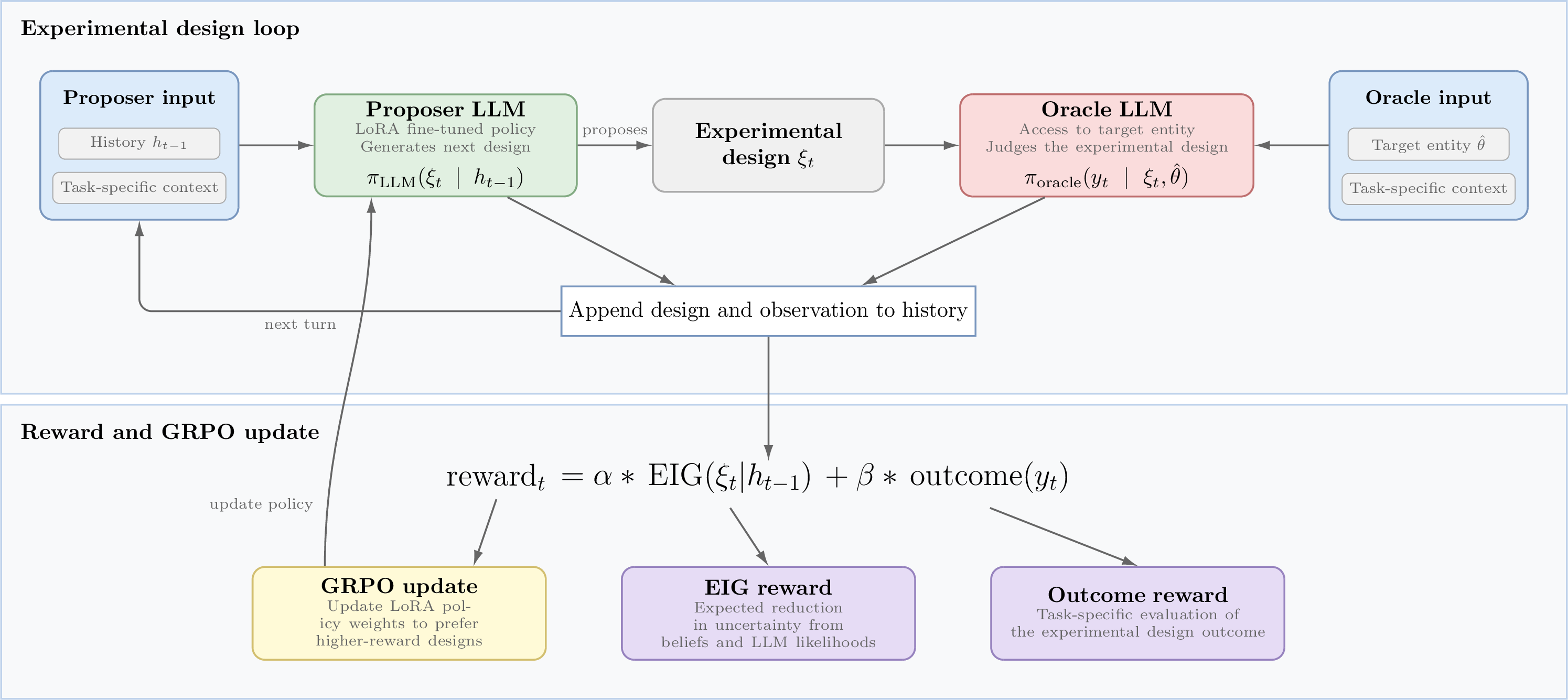
We consider a multi-turn interaction environment, in which the Proposer LLM agent is tasked with uncovering a latent target quantity \(\hat{\theta}\in\Theta\) through a budget of \(T\) sequential experimental designs \(\xi\in\Xi\). The environment is initialised with a task-specific prompt which defines the search space. Over a trajectory \(\tau=\{(\xi_k,y_k)\}^{k=T}_{k=1}\), the agent interacts with the environment, modelled by the frozen and independent Oracle LLM, through experimental designs \(\xi\) and receives its outcomes \(y\in\mathcal{Y}\). The interaction history at step \(t\) is denoted by \(h_{t-1}=\{(\xi_k,y_k)\}^{k=t-1}_{k=1}\), with \(h_0\) being the initial task-specific prompt. In this setting, we treat the Proposer LLM agent as our sequential BED policy \(\pi_{\text{LLM}}(\cdot|h_{t-1})\), from which experiments are sampled based on the accumulated context. We then use the Proposer LLM to generate beliefs and compute likelihoods \(p_{\text{LLM}}(y_t|\theta, \xi_t)\) to estimate the EIG for each proposal. An outcome-based reward is computed from the corresponding experimental outcomes, and together these two components define the reward signal in our multi-turn GRPO fine-tuning setup. Figure 1 provides a high-level overview of the approach, while the following subsections detail the specific implementation evaluated in this work.
4.1 Training Environment↩︎
In this study, we implement our training procedure using the 20 Questions game environment, which has several desirable properties in this context. First, 20 Questions forms a natural instantiation of the BED framework in which the questions posed by the LLM are themselves the experimental designs \(\xi_t\), and the answers are the corresponding experimental outcomes \(y_t\). Additionally, the binary experimental outcome space (i.e. “yes” or “no”) allows for an efficient estimation of the EIG through the Rao-Blackwellised estimator in 2 . Finally, [23] have shown that succeeding in 20 Questions requires good planning to efficiently partition the hypothesis space before deductive reasoning can be used to produce educated guesses in later turns. This generic planning-oriented structure makes the task a useful proxy for learning capabilities that may transfer to other information gathering tasks.
The resulting environment is implemented as an interaction between the Proposer LLM, which is fine-tuned, and a separate frozen Oracle LLM. At each turn, the Proposer receives the task category together with the accumulated question-answer history and generates a question or guess. The Oracle, which has access to the hidden target entity, evaluates this proposal and returns a binary answer, either “Yes” or “No”, unless the Proposer has correctly identified the target, in which case the Oracle returns “Correct” and the interaction terminates. For non-terminal turns, the resulting question-answer pair is appended to the history and the interaction continues until either the target is identified or the budget of \(T=20\) turns is exhausted.
4.2 Reward↩︎
Effective information gathering requires the ability to both design maximally informative experiments and identify when enough information has been acquired to identify the hidden entity and act optimally. We argue that these are two distinct skills, which motivates two separate components for the reward signal. For each experimental design (e.g. a question in 20 Questions) generated in the GRPO rollout, we calculate two reward components: EIG and outcome reward. These two signals are complementary. EIG provides dense, turn-level feedback on question quality but carries no signal on whether information gathering ultimately succeeds, while the outcome-based reward drives goal-directed behaviour but suffers from sparse credit assignment in long-horizon settings. For 20 Questions specifically, the outcome reward encourages the model to guess the hidden entity using as few questions as possible, while EIG encourages asking maximally informative questions.
The outcome reward, denoted \(r_{\mathrm{out}}(y_t)\), consists of a step-wise penalty for all questions that lead to a non-terminal state and a large positive reward if the questioner has correctly guessed the hidden entity.
To calculate the EIG for a given question \(\xi_t\), we use the approach introduced by [9] and visualized in Figure 2. At each turn, we sample beliefs \(\theta\sim p_{\text{LLM}}(\cdot|h_{t-1})\) from the Proposer LLM to create a belief set based on the current conversation history. This set is then filtered to ensure that only coherent beliefs, which are consistent with the previous questions and answers, are retained. If the resulting belief set is too small, we perform up to three rounds of belief regeneration to ensure a large enough set. We denote the resulting belief set at turn \(t\) formed from this process as \(\Theta_t\). Afterwards, we uniformly sample \(N\) beliefs \(\theta_n\in\Theta_t\) and query the Proposer LLM to obtain the likelihoods for each sampled belief, \(p_{\text{LLM}}(y_t|\theta_n, \xi_t)\), which are used to estimate the question’s EIG via the Rao-Blackwellised estimator in 2 . We scale the EIG reward by \(1 / \ln(2)\) to obtain a normalized scalar, \(r_{\mathrm{EIG}}(\xi_t,\Theta_t)\), within the \([0,1]\) range.
4.3 Multi-Turn GRPO↩︎
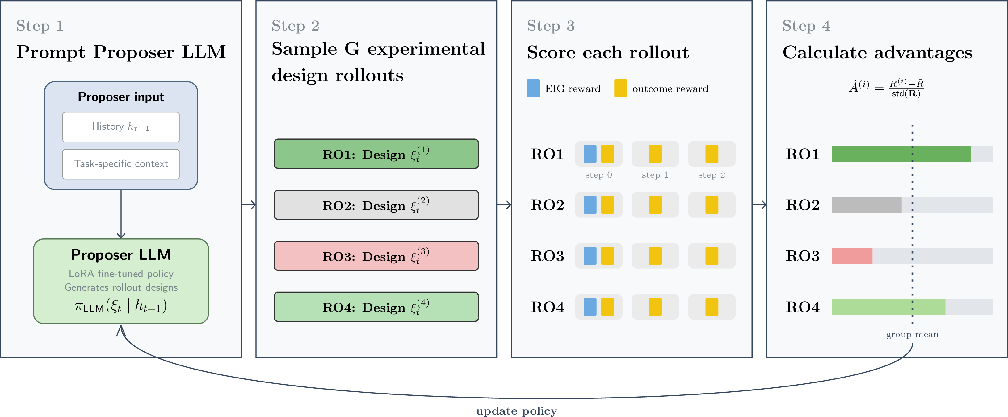
We extend the default GRPO formulation [13] to the multi-turn setting. At each training step, a starting state consisting of the task category and the interaction history up to that turn, \(h_{t-1}\), is sampled from the prompt dataset outlined in 4.5. From this state, the Proposer LLM generates \(G\) independent policy rollouts by sampling multiple consecutive question-answer pairs within each rollout. A high-level overview is shown in Figure 3. For each rollout, we compute the scalar reward described in Section 4.2 using
\[R_t = \frac{\alpha}{\mathcal{Z}_E} \sum_{k=0}^{E-1} \gamma_{\mathrm{EIG}}^{k}\, r_{\mathrm{EIG}}(\xi_{t+k},\,\Theta_{t+k}) + \frac{\beta}{\mathcal{Z}_O} \sum_{k=0}^{O-1} \gamma_{\mathrm{out}}^{k}\, r_{\mathrm{out}}(y_{t+k}),\]
where \(\alpha, \beta\) are weighting constants, \(\gamma_{\mathrm{EIG}}, \gamma_{\mathrm{out}} \in (0,1]\) are discount factors, and \(E, O\) correspond to the rollout horizon for the EIG and outcome-based reward, respectively. The normalization constants \(\mathcal{Z}_E\) and \(\mathcal{Z}_O\) ensure that different rollout horizons for EIG and outcome-based rewards do not lead to varying reward magnitudes. For a horizon \(H\) and discount factor \(\gamma\), we define
\[\mathcal{Z}(H,\, \gamma) = \sum_{k=0}^{H-1} \gamma^{k} = \begin{cases} H & \text{if } \gamma = 1 \\[4pt] \dfrac{1 - \gamma^{H}}{1 - \gamma} & \text{otherwise}. \end{cases}\]
In our experiments, we use \(E = 1\) and \(O = 3\), i.e. the EIG reward is calculated only with respect to the first question in each rollout, whereas the outcome reward also considers the two subsequent questions. This favours questions that maximize EIG at the current turn, while increasing the probability of a correct guess within three turns. After obtaining the rewards for each question, we calculate the average group return and individual rollout advantages, which are used to update the LoRA [24] adapters of the questioner model.
4.4 Learning Curriculum↩︎
In preliminary experiments, we observed that the Proposer LLM initially rarely makes specific guesses. To encourage this behaviour, we employ a learning curriculum strategy in which the model is first trained without the EIG reward (\(\alpha = 0\)), before subsequently introducing the EIG signal. This curriculum increases the frequency of hypothesis-seeking questions, which contain specific guesses, relative to constraint-seeking questions that probe the characteristics of the hidden entity.
4.5 GRPO Prompt Dataset↩︎
At the start of each training episode, we randomly sample \(n\) target entities from a category-entity list to generate a 20 Questions self-play dataset between the Proposer and Oracle. Each state in this dataset, consisting of the entity’s category and the Q/A history up to question \(t-1\), then serves as input for GRPO rollouts starting at question \(t\).
5 Experiments↩︎
5.1 Setup↩︎
To evaluate our method, we train on the 20 Questions task and assess both in-distribution and out-of-distribution performance. We use Qwen2.5-7B-Instruct and Qwen2.5-14B-Instruct as Proposer LLMs and Qwen2.5-72B-Instruct as the Oracle LLM [25]. For training, we construct a list of 1,000 target entities spanning 20 categories. This list was generated with Claude Opus 4.7 [26] using [prompt:training_dataset_generation] and manually reviewed to ensure quality. We train a LoRA adapter on this dataset following the approach in 4, with hyperparameters listed in 2.
We evaluate in-distribution performance on two held-out categories and out-of-distribution performance on MediQ [14], a medical information-seeking benchmark. We further verify that improved information-seeking capabilities do not come at the cost of degraded general language abilities, as measured on three standard LLM benchmarks.
5.2 20 Questions↩︎
We evaluate the fine-tuned models on two held-out categories, animals and plants, each comprising 100 entities not seen during training. The animal entities are drawn from [9] and the plant entities are a subset of those used by [8]. The full lists are provided in [box:animals95dataset] [box:plants95dataset]. We compare against the instruction-tuned base model and our reimplementation of BED-LLM [9], [27].
5.2.0.1 Success rate.
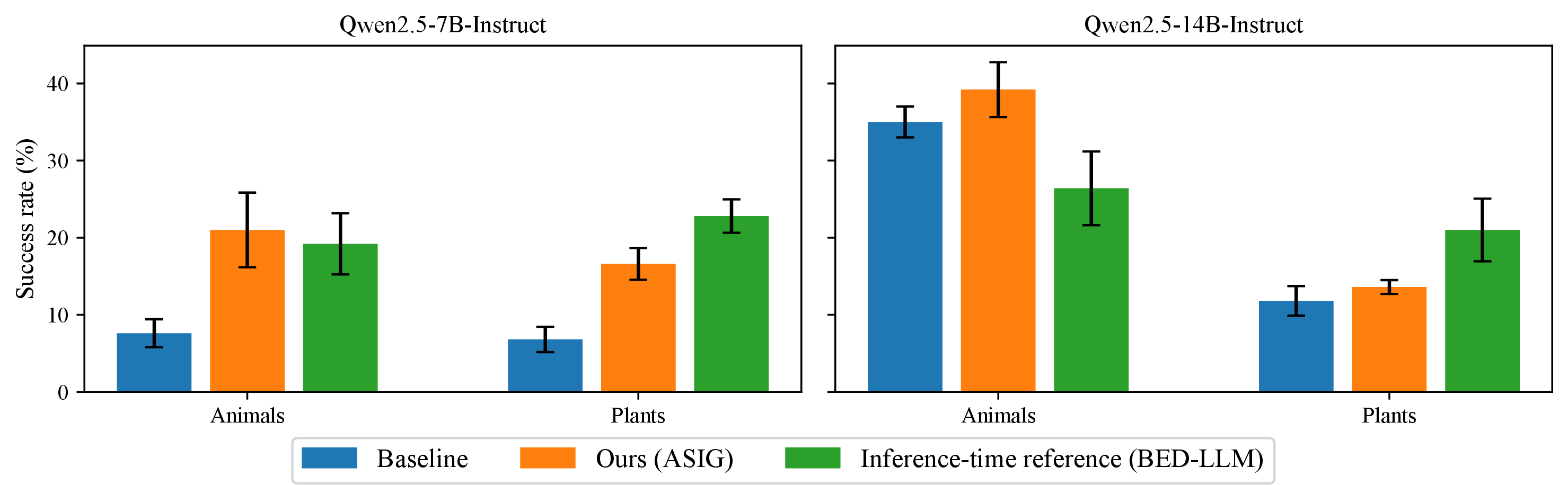
4 shows the success rate across model sizes and evaluation categories, measured as the fraction of games in which the questioner identifies the hidden entity within the 20 question budget. On the 7B model, ASIG more than doubles the success rate over the baseline and surpasses BED-LLM on the animals category. On the 14B model, ASIG improves over the baseline by 4.2 and 1.8 percentage points on animals and plants, respectively. BED-LLM performs better on the 14B plants category but degrades on the animals category, falling below both ASIG and the baseline, suggesting that it does not generalise robustly across settings despite requiring an order of magnitude more inference-time compute. 8 in the Appendix further shows that ASIG identifies the target entity earlier than the baseline, requiring fewer questions on average. Qualitative examples comparing baseline and ASIG on the same target entity are shown in [box:game95fir] [box:game95honey95bee] in the Appendix.
5.2.0.2 Behavioural analysis.
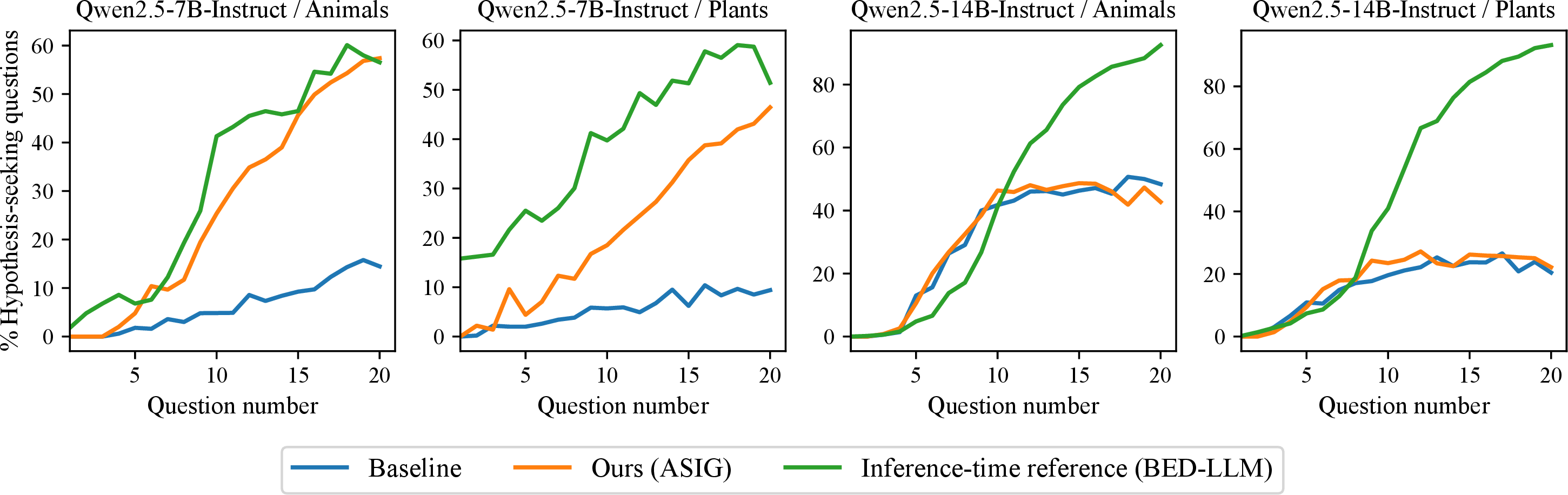
To better understand the strategies learned by ASIG, we classify each question as either constraint-seeking (asking about the entity’s characteristics to narrow down candidates) or hypothesis-seeking (making a specific guess about the target), following the taxonomy of [4]. 5 shows the fraction of hypothesis-seeking questions across turns. For the 7B model, ASIG consistently exceeds the baseline across both categories, committing to explicit guesses earlier in the game.
For the 14B model, ASIG’s hypothesis-seeking rate closely tracks the baseline. This likely reflects the stronger prior capabilities of the 14B model, which requires less behavioural adaptation to benefit from fine-tuning. BED-LLM achieves the highest overall rate, but this is partly driven by hard-coded guessing logic that forces explicit guesses once the belief set falls below three candidates, which ASIG does not rely on.
| Model | Variant | Accuracy (%) \(\uparrow\) | Voluntary accuracy (%) \(\uparrow\) | Overconfidence rate (%) \(\downarrow\) | Underconfidence rate (%) \(\downarrow\) |
|---|---|---|---|---|---|
| Qwen2.5-7B-Instruct | Baseline | 46.7 | 50.1 | 36.1 | 10.6 |
| Ours (ASIG) | 47.6 | 51.8 | 33.4 | 11.7 | |
| Qwen2.5-14B-Instruct | Baseline | 54.1 | 64.6 | 20.7 | 16.5 |
| Ours (ASIG) | 54.2 | 63.0 | 22.2 | 16.4 |
5.2.0.3 Inference-Time Efficiency.
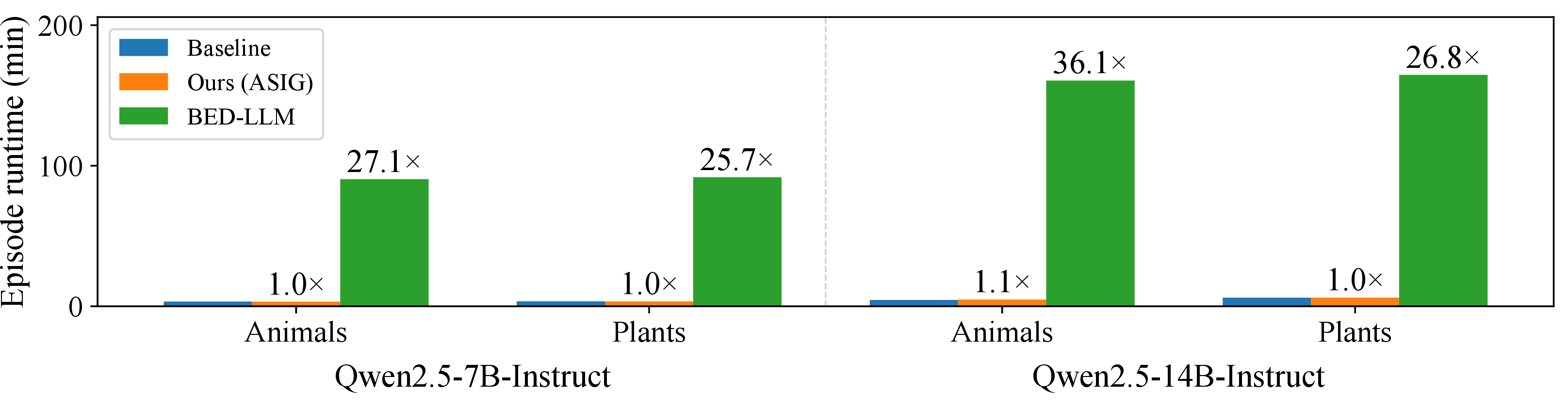
By amortising the Bayesian experimental design computation into the model weights, ASIG incurs the same inference cost as the base LLM. Notably, this makes ASIG between 25x and 36x faster than BED-LLM (6), which must perform explicit belief sampling and EIG maximisation at every turn. This efficiency gain makes ASIG considerably more applicable to real-world settings where latency and compute are constrained.
5.3 Generalization to Medical Information Seeking↩︎
To assess out-of-distribution performance, we evaluate our fine-tuned models on MediQ [14], a benchmark that simulates a clinical interaction in which a doctor elicits information from a patient through follow-up questions before answering a multiple-choice clinical question. At each turn, a doctor agent uses an abstention module to decide whether sufficient information has been gathered to answer or whether to ask another question. We use our fine-tuned Qwen2.5-7B and Qwen2.5-14B models from the 20 Questions task as the doctor and Qwen2.5-72B-Instruct as the patient, which responds based on a provided patient record.
We compare each fine-tuned model to its base counterpart across four metrics: accuracy (overall success rate), voluntary accuracy (success when the model voluntarily committed to an answer), overconfidence (incorrect committed answers), and underconfidence (continued questioning despite having enough information to answer correctly).
Our 7B model improves accuracy and voluntary accuracy by 0.9 and 1.7 percentage points, respectively. The overconfidence rate drops from 36.1% to 33.4%, at a slight cost of 1.1 percentage points in underconfidence. Results are more mixed for the 14B model: accuracy remains essentially unchanged, voluntary accuracy decreases slightly from 64.6% to 63.0%, and overconfidence increases marginally by 1.5 percentage points.
Overall, ASIG transfers well to the medical domain at the 7B scale. The gains in voluntary accuracy and reduction in overconfidence align with our earlier finding that fine-tuning encourages more deliberate hypothesis-seeking, here reflected in the model’s improved judgement about when to commit to an answer. The mixed 14B results are consistent with the weaker behavioural adaptation observed in the hypothesis-seeking analysis, suggesting that the larger model’s stronger prior capabilities leave less room for fine-tuning to induce meaningful behavioural change.
5.4 Capability Retention↩︎
To ensure that fine-tuning does not degrade performance on other tasks or lead to failure modes such as catastrophic forgetting, we evaluate the baseline and fine-tuned models on three standard LLM benchmarks: ARC-Challenge [28], HellaSwag [29], and MMLU [30], [31]. As shown in 9 in the Appendix, the fine-tuned models achieve near-identical scores to the base models across all three benchmarks, confirming that improved information-seeking abilities do not come at the cost of general language capabilities.
6 Conclusion↩︎
We introduced ASIG, a multi-turn GRPO-based fine-tuning method that amortises BED into LLM policies for sequential information gathering. By shifting information-seeking behaviour from inference-time optimisation into model weights, ASIG improves task performance while substantially reducing the computational overhead of sequential BED at deployment time.
Across two model scales, fine-tuning on 20 Questions consistently improves information-gathering performance on held-out categories, outperforming BED-LLM, a competitive inference-time BED baseline, in two of four settings while reducing inference cost by over \(25\times\) overall. We further show partial transfer to MediQ, where ASIG improves clinical reasoning accuracy at the 7B scale without measurable degradation on standard language-understanding benchmarks. These results suggest that amortising information-seeking behaviour into model weights provides a practical and scalable approach to test-time information acquisition in LLMs.
Future work includes disentangling the effects of EIG and outcome-based rewards, evaluating broader sequential information-gathering benchmarks, and extending ASIG to reasoning models generating intermediate reasoning steps.
Acknowledgements↩︎
We thank Tobias Bretschneider for his contributions to the development of the codebase and to the broader project. We are also grateful to Ari Weinstein for insightful discussions and valuable feedback throughout the course of this work. We thank Linus Filbry for making his BED-LLM implementation publicly available and for helpful discussions regarding its implementation details. Experiments reported in this work were supported by computational resources provided by the Ellison Institute of Technology, Oxford. The authors would also like to acknowledge the use of the University of Oxford Advanced Research Computing (ARC) facility in carrying out this work (DOI: 10.5281/zenodo.22558).
7 Hyperparameters↩︎
| Symbol | Name | Value |
|---|---|---|
| BED-LLM inference | ||
| \(N\) | Belief set size | 15 |
| \(M\) | Candidate questions per turn | 15 |
| \(\tau_f\) | Belief filter threshold | 0.2 |
| \(T_{\text{gen}}\) | Generation temperature (beliefs & candidates) | 1.3 |
| \(T_a\) | Answer temperature (likelihood) | 0.7 |
| — | Max regeneration rounds | 3 |
| — | Monte Carlo samples for EIG | 15 |
| — | Retain consistent old beliefs | true |
| Reward | ||
| \(\alpha\) | EIG reward weight curriculum | \(0.0 \xrightarrow{\text{epoch 20}} 1.0\) |
| \(\beta\) | Outcome reward weight | 1.0 |
| \(r_{\text{out}}(\text{Correct})\) | Correct-guess reward | +5 |
| \(r_{\text{out}}(\text{Yes/No})\) | Step penalty | -1 |
| \(N\) | Belief set size (reward model) | 15 |
| \(\tau_f\) | Belief filter threshold (reward model) | 0.2 |
| \(T_a\) | Answer temperature (reward model) | 0.7 |
| \(E\) | EIG rollout horizon | 1 |
| \(O\) | Outcome rollout horizon | 3 |
| \(\gamma_{\text{eig}}\) | EIG discount factor | 1.0 |
| \(\gamma_{\text{out}}\) | Outcome discount factor | 0.9 |
| GRPO training | ||
| — | Epochs | 40 |
| — | Initial learning rate | \(2 \times 10^{-6}\) |
| \(\beta_{\mathrm{KL}}\) | KL penalty coefficient | 0.0 |
| \(G\) | Group size (completions per prompt) | 8 |
| — | Per-device batch size | 2 |
| — | Gradient accumulation steps | 8 |
| — | Max completion length (tokens) | 128 |
| — | Sampled entities per epoch | 100 |
| — | Dataset refresh (epochs) | 1 |
| — | Questions budget per game | 20 |
| LoRA | ||
| \(r\) | Rank | 32 |
| \(\alpha_{\text{LoRA}}\) | Scaling factor | 64 |
| — | Dropout | 0.05 |
| — | Target modules | all attention + MLP projections |
8 Prompts↩︎
Proposer Agent System Promptnaive_agent_system You are playing a game of 20 Questions. Using all previous questions and answers:
Generate the best question to help identify the target {category}. The question should be phrased so the answer is Yes or No. Print only the question - no numbering, punctuation, or extra text.
Oracle Answerer System Promptoracle_answerer_system You are playing the oracle answerer in a game of 20 Questions. The questioner has to guess a secret entity from the category: {category}. Your secret entity is: {entity}
CRITICAL INSTRUCTIONS:
1. If the question directly identifies, names, or guesses “{entity}" as the answer, respond ONLY with the word "Correct"
2. For yes/no questions about properties or characteristics, respond ONLY with "Yes" or "No"
3. Never add explanations, extra words, or punctuation
Examples:
- "Is it {entity}?" -> "Correct"
- "Is it a {entity}?" -> "Correct"
- "Are you thinking of {entity}?" -> "Correct"
- "I think it’s {entity}" -> "Correct"
- "Is the {category} a {entity}?" -> "Correct"
- "Is it bigger than a car?" -> "Yes" or "No" (depending on {entity})
- "Can you find it indoors?" -> "Yes" or "No" (depending on {entity})
- "Is it man-made?" -> "Yes" or "No" (depending on {entity})
- "Is it alive?" -> "Yes" or "No" (depending on {entity})
Likelihood Model System Promptlikelihood_model_system You are playing the answerer in a game of 20 Questions. Your chosen entity is: {hypothesis}
When asked a question, you must reply exactly “Yes" or”No", depending on if your chosen entity fulfills the question.
Question Classifier System Promptquestion_classifier_system You are classifying questions from a 20 Questions game.
C - constraint-seeking: narrows the space of possible entities by asking about properties or categories (e.g. "Is it a mammal?", "Is it bigger than a car?")
H - hypothesis-seeking: asks whether the target IS a specific entity (e.g. "Is it a cat?", "Is it the Eiffel Tower?")
U - unknown: the question is ambiguous or does not fit either category
Reply with ONLY the single letter: C, H, or U.
Training Dataset Generation Prompttraining_dataset_generation Role: You are a curator building a high-quality entity dataset for a 20 Questions game.
Task: Generate \(\sim\)50 entities for each of the categories listed below. Each entity must be guessable through \(\sim\)20 yes/no questions by an average adult player.
Categories & quantities:
Musical instrument
Fruit
Organ
Profession
City
Clothing
Game
Furniture
Author
Vegetable
Sport
Vehicle
Electronic device
TV show
Celebrity
Food chain
University course
Monument
Cooking equipment
River
Quality criteria - each entity must be:
Recognizable - known to a general adult audience, not requiring specialist knowledge.
Concrete & unambiguous - a single, well-defined referent (e.g., "elephant," not "large mammal").
Distinguishable - possesses a clear set of yes/no-answerable properties (size, habitat, function, era, material, etc.).
Non-trivial - avoid items so generic they’re guessed in 3 questions ("dog") or so obscure they’re unguessable.
Diverse within category - span subtypes, regions, eras, and difficulty levels; no near-duplicates.
Output format: CSV
For reference, attached are example lists for the animals and plants category. Generate entities with a similar level of difficulty.
9 20 Questions Evaluation Datasets↩︎
Animals datasetbox:animals95dataset
4
African elephant
Bengal tiger
Bald eagle
Blue whale
Red kangaroo
Giant panda
Snow leopard
Green sea turtle
American alligator
Bottlenose dolphin
Emperor penguin
Great white shark
Golden poison frog
Honey bee
Monarch butterfly
Okapi
Chimpanzee
Arctic fox
Komodo dragon
Giraffe
Cheetah
Hammerhead shark
Axolotl
Orca
Puffin
Red panda
Platypus
Rhinoceros
Tasmanian devil
Wombat
Sloth
Blue-ringed octopus
Manatee
Narwhal
Sea otter
Coral snake
King cobra
Harpy eagle
Lemur
Koala
Aye-aye
Snowy owl
Elk
Wolverine
Caracal
Cassowary
Quokka
Pangolin
Saiga antelope
Galápagos tortoise
Sumatran orangutan
Red-eyed tree frog
European badger
Moose
African grey parrot
Scarlet macaw
Black mamba
Albatross
Humpback whale
Dugong
Anaconda
Kookaburra
Coyote
Brown bear
Golden jackal
Capybara
Ibex
Japanese macaque
Kiwi
Leafcutter ant
Mantis shrimp
Ocelot
Peregrine falcon
Quetzal
Raccoon
Sand cat
Tarantula
Uakari
Vicuña
Wildebeest
Rock hyrax
Yak
Zebra
Blue dragon nudibranch
Chinchilla
Dhole
Electric eel
Flying fox
Gharial
Horseshoe crab
Indigo bunting
Jerboa
Kakapo
Lionfish
Markhor
Nautilus
Olive baboon
Pika
Quoll
Rosy boa
Plants datasetbox:plants95dataset
4
Rose
Oak
Pine
Palm
Redwood
Elm
Cedar
Juniper
Hickory
Willow
Bamboo
Hemlock
Poplar
Birch
Cypress
Magnolia
Eucalyptus
Maple
Fir
Beech
Mahogany
Spruce
Dogwood
Yew
Larch
Aspen
Sycamore
Hawthorn
Holly
Marigold
Lily
Primrose
Hyacinth
Lotus
Crocus
Anemone
Carnation
Iris
Bluebell
Lavender
Orchid
Poppy
Pansy
Dandelion
Sunflower
Narcissus
Calendula
Fuchsia
Jasmine
Chrysanthemum
Lilac
Ranunculus
Azalea
Gladiolus
Hibiscus
Daffodil
Petunia
Snowdrop
Begonia
Freesia
Cornflower
Hellebore
Dahlia
Peony
Violet
Camellia
Hollyhock
Alyssum
Geranium
Gardenia
Scilla
Primula
Tuberose
Poinsettia
Amaryllis
Impatiens
Mimosa
Forsythia
Delphinium
Bellflower
Aster
Trillium
Hydrangea
Zinnia
Agave
Aloe
Cactus
Saguaro
Fern
Philodendron
Cyclamen
Lupin
Rudbeckia
Yarrow
Foxglove
Wisteria
Clematis
Honeysuckle
Allium
Viburnum
10 Extended Results↩︎
Figure 7: 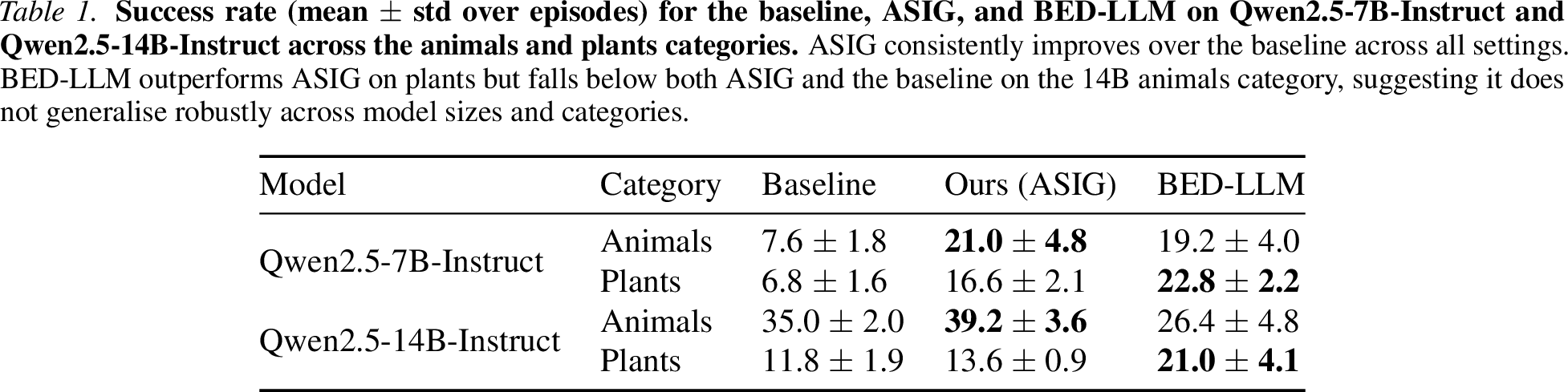 .
.
Figure 8: 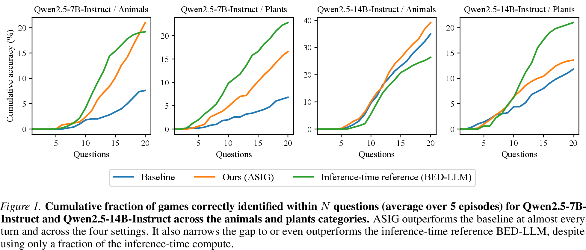 .
.
Figure 9: 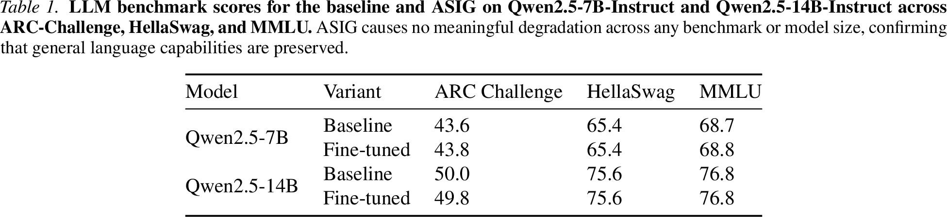 .
.
11 Example Games↩︎
Figure 10: 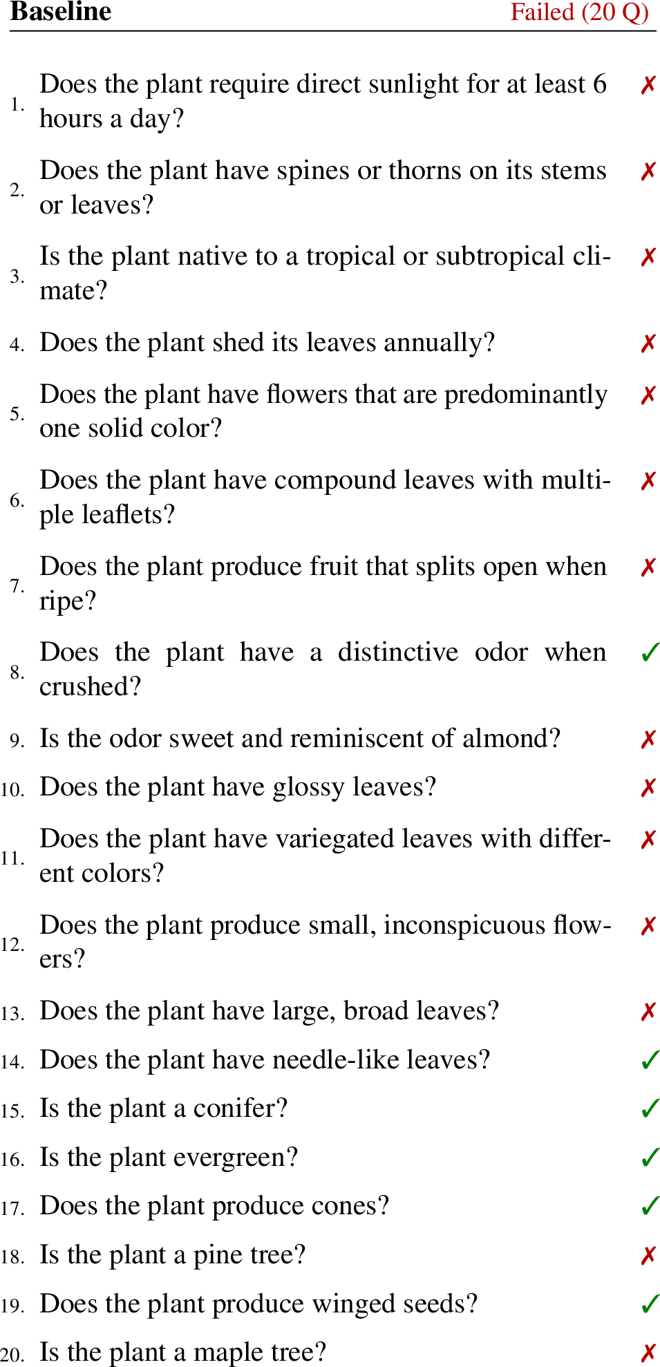 .
.
Figure 11: 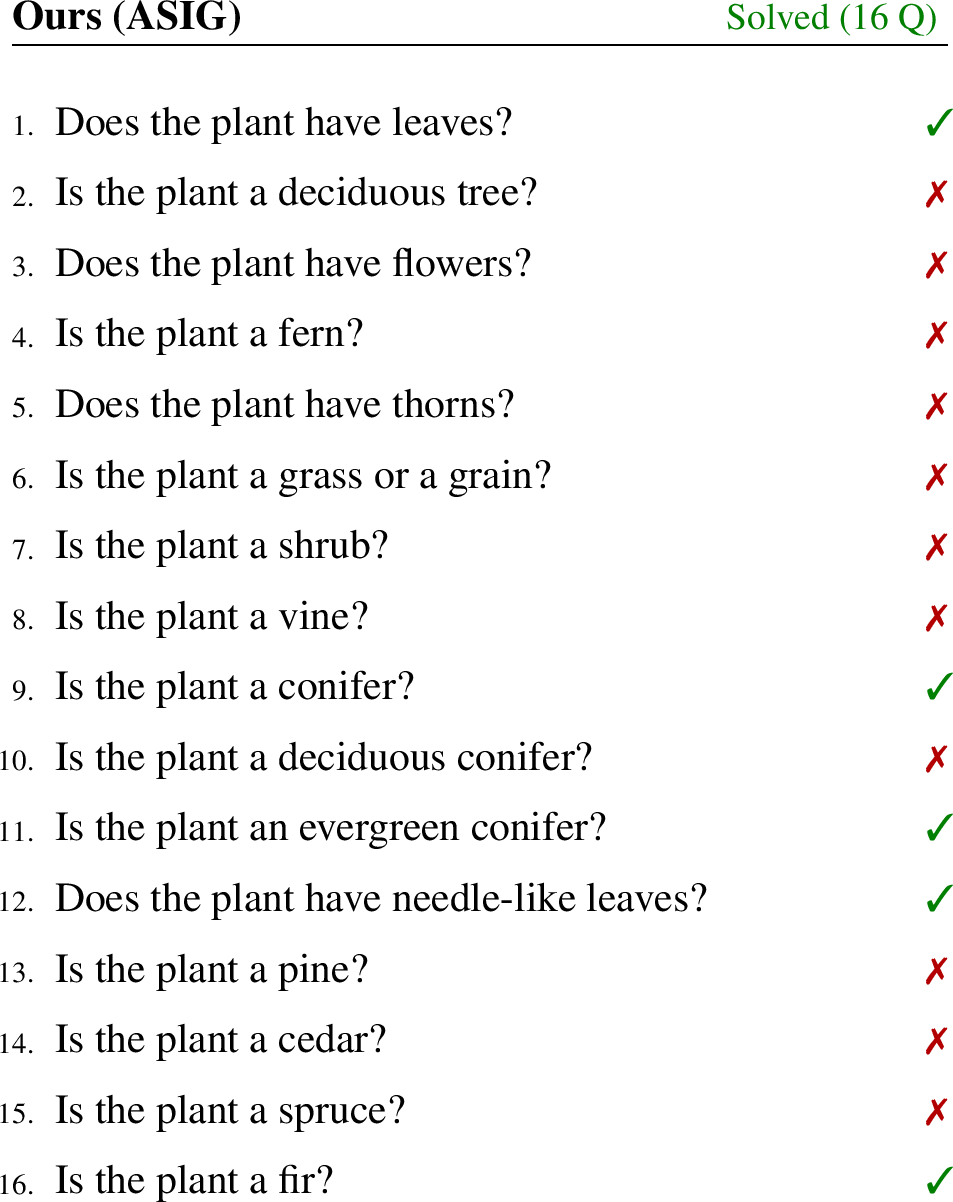 .
.
Figure 12: 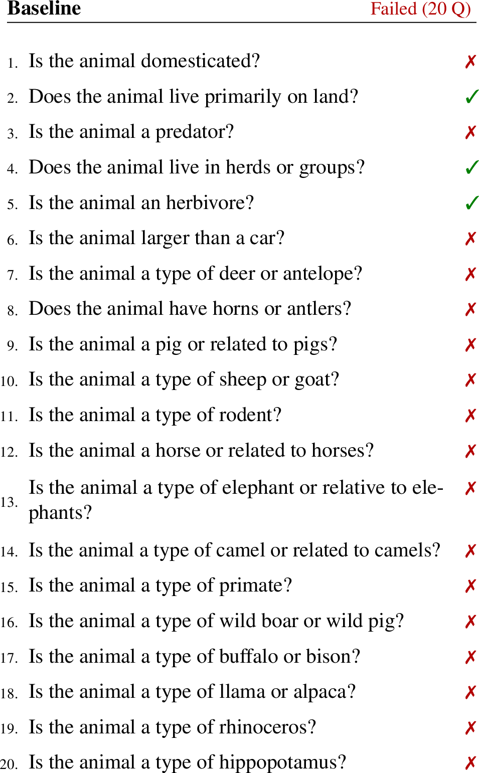 .
.
Figure 13:  .
.
References↩︎
This assumes that \(y_t\) is independent of \(h_{t-1}\) given \(\theta\) and \(\xi_t\), which is the case for our 20 Questions training environment.↩︎