Accelerating droplet-laden Stokes flow simulations with hierarchical surrogate modeling
July 03, 2026
Abstract
We present a surrogate modeling strategy for Stokes flows with liquid droplets suspended in a carrier fluid. Our approach is based on a multi-fidelity framework. At the lowest fidelity, droplets are treated as passive tracers, neglecting their influence on the ambient flow field. Building on this approximation, we derive a PDE that represents the current modeling error. This error equation is then solved approximately to correct the flow field and the procedure is iterated. Two fidelities are employed in an alternating fashion: Stokes flow in the absence of droplets and flow around a single droplet in free space. By systematically combining these models, the method captures droplet-flow, droplet-boundary, and droplet-droplet interactions. For geometrically similar droplets, we further develop an efficient offline-online strategy that exploits this structure by reusing precomputed single-droplet solutions. Numerical experiments demonstrate the accuracy and efficiency of the proposed surrogate in a variety of tests, including scenarios with up to \(10^4\) droplets. Notably, we show that the proposed surrogate achieves substantially reduced computational cost compared to fully resolved multi-fluid simulations with state-of-the-art software.
1 Introduction↩︎
Multiphase flow systems arise in a wide range of applications, including microfluidics, porous media, ink-jet printing and biomedical applications. Accurate predictions for such systems increasingly rely on high-fidelity computer simulations[1]–[4]. In this work, we study incompressible multiphase Stokes flow involving a large number of immiscible droplets suspended in a carrier fluid.
From a computational point of view, a key difficulty arises when droplets are many and become highly concentrated or approach boundaries. Standard discretization techniques can only capture the dynamics in such regimes by resolving the narrow interfacial gaps and near-boundary interactions, making the resulting numerical schemes computationally demanding.
For example, standard finite-element methods rely on fine meshes that conform to the interfaces and therefore require repeated remeshing as the interfaces evolve. Unfitted methods such as CutFEM avoid remeshing but still require fine local resolution to accurately capture narrow gaps [5], [6]. Boundary integral methods face similar challenges, requiring specialized quadrature schemes and fine resolution around interfaces to accurately evaluate near-singular integrals arising from closely interacting droplets and boundaries [7].
Alternative particle-based methods, such as smoothed particle hydrodynamics [8] and the moving particle semi-implicit method [9], [10], eliminate the need for mesh generation and remeshing. However, accurately resolving near-contact interactions still requires sufficiently fine particle resolutions. Moreover, these methods typically achieve lower accuracy than high-order finite-element or boundary-integral methods and often require careful tuning of numerical parameters (such as kernel functions and stabilization terms) to ensure numerical stability.
An additional challenge arises as the interfaces evolve in time, since the flow problem must be approximated and solved on a sequence of changing geometries. In scenarios with many droplets, the fine spatial resolution required to capture near-contact interactions usually leads to expensive simulations. In this work, we present a surrogate model that enables efficient prediction of droplet evolution, even in densely packed, time-varying configurations.
1.1 Target problem↩︎
We consider an incompressible multiphase Stokes system in a bounded Lipschitz domain \(\Omega\subset\mathbb{R}^d\), \(d\in\{2,3\}\). The system consists of \(M\geq1\) droplets of immiscible fluid in a surrounding carrier fluid. The droplets occupy the region3 \(\overline{\Omega_B}\subset\Omega\), which consists of \(M\) connected components (the “droplets”). Each droplet is bounded by a smooth interface, and the surrounding fluid occupies \(\Omega_F=\Omega\setminus\overline{\Omega_B}\). The union of all droplet interfaces is denoted by \(\Gamma=\partial\Omega_B\). To represent the different fluid properties, we introduce a piecewise constant viscosity field \(\mu:\Omega\to\mathbb{R}_{>0}\), with jumps across the droplet interfaces \(\Gamma\).
Dirichlet and Neumann boundary conditions are prescribed on \(\Gamma_D\subset\partial\Omega\) and \(\Gamma_N=\partial\Omega\setminus\Gamma_D\), respectively, although other boundary conditions may also be considered. A schematic illustration of the computational domain and its boundaries is shown in 1. Across the interfaces \(\Gamma\), the velocity is continuous, ensuring conservation of mass, while the jump in the normal stress balances the surface tension force.

The interfaces evolve with the fluid velocity. At each time \(t \in [0,T]\), the flow satisfies the Stokes equations: \[\label{eq:cutfemtime} \begin{cases} \dot{\mathbf{x}}(t)=\mathbf{u}(t) & \text{on } \Gamma(t),\\ -\nabla\cdot{\boldsymbol{\sigma}}(\mathbf{u}(t),p(t);\mu)=\mathbf{f}& \text{in } \Omega\setminus\Gamma(t),\\ \nabla\cdot\mathbf{u}(t)=0 & \text{in } \Omega\setminus\Gamma(t),\\ \left\llbracket\mathbf{u}(t)\right\rrbracket=\mathbf{0}& \text{on } \Gamma(t),\\ \left\llbracket{\boldsymbol{\sigma}}(\mathbf{u}(t),p(t);\mu)\mathbf{n}\right\rrbracket=\gamma\kappa\mathbf{n}& \text{on } \Gamma(t),\\ \mathbf{u}(t)=\mathbf{g}_D& \text{on } \Gamma_D,\\ {\boldsymbol{\sigma}}(\mathbf{u}(t),p(t);\mu)\mathbf{n}=\mathbf{g}_N& \text{on } \Gamma_N, \end{cases}\tag{1}\] with \(\mathbf{x}(t)\) denoting the position of the interface, whereas \(\mathbf{u}\) and \(p\) denote the velocity and pressure fields, respectively. Furthermore, \({\boldsymbol{\sigma}}(\mathbf{u},p;\mu)=2\mu{\boldsymbol{\varepsilon}}(\mathbf{u})-p\mathrm{I}\) is the viscous stress tensor, \(\gamma\) is the (piecewise constant) surface tension coefficient, \(\kappa:\Gamma\to\mathbb{R}\) is the mean curvature of the interface \(\Gamma\) and \(\mathbf{n}\) is the unit normal to the interface (pointing towards \(\Omega_F\)) and on the outer boundary (pointing outwards). We use double square brackets to denote jumps across \(\Gamma\), i.e., \(\left\llbracket\mathbf{u}\right\rrbracket:=\mathbf{u}|_{\Omega_F}-\mathbf{u}|_{\Omega_B}\).
The volume forcing term is \(\mathbf{f}\in[H^{-1}(\Omega)]^d\), whereas the Dirichlet and Neumann boundary data are given by \(\mathbf{g}_D\in[H^{1/2}(\Gamma_D)]^d\) and \(\mathbf{g}_N\in[H^{-1/2}(\Gamma_N)]^d\), respectively4. For simplicity, we assume that the boundary data are time-independent, so that the only time dependence in 1 arises through the evolution of the interface \(\Gamma(t)\). This assumption can be relaxed, as the main challenge lies in the treatment of the evolving interface \(\Gamma(t)\). Assuming that \(\Gamma(t)\) is sufficiently smooth, there exists a weak solution \((\mathbf{u}(t),p(t))\in [H^1(\Omega)]^d\times L^2(\Omega)\) for each fixed \(t\in[0,T]\).
The linearity (in \(\mathbf{u}\) and \(p\)) of the multiphase Stokes problem 1 makes it particularly attractive for the development of compact surrogate models. While the more general multiphase Navier-Stokes equations are required when fluid inertia cannot be neglected, their nonlinear nature introduces substantial additional complexity. At the same time, the Stokes setting accurately describes a broad class of low-Reynolds-number multiphase flows and is already sufficiently rich to capture the geometric and interfacial challenges that motivate this work.
1.2 Surrogate modeling↩︎
There is growing interest in surrogate models that provide accurate and efficient predictions of multiphase flows, particularly in regimes where fully resolved simulations are computationally challenging. Machine learning (ML) algorithms are increasingly employed to construct such surrogates, with the aim of replacing expensive high-fidelity simulations with computationally efficient predictions. ML-based approaches have been used, for example, to predict droplet breakup [11], flow fields around obstacles such as spinning spheres [12], pairwise hydrodynamic interactions in Stokes flows [13], and the spatiotemporal evolution of microstructures [14]. Most closely related to the problem considered here is the machine-learning-augmented reduced model proposed in [15], which also studies systems of many particles interacting through Stokes flow.
For the stationary Stokes problem with rigid particles, we also mention the recent work [16], which combines the method of fundamental solutions with the method of images to obtain a computationally cheaper alternative to standard boundary integral formulations and demonstrates simulations with up to 2000 fixed spheres.
In regimes with many droplets and small interfacial separations, existing high-fidelity solvers require extreme mesh refinement near narrow gaps, while existing ML surrogates often lack the physical transparency needed to guarantee reliability and accuracy, particularly outside the regimes represented by the training data. To address these challenges, this work introduces a novel hierarchical, physics-informed surrogate modeling framework for the multiphase Stokes problem 1 . The core ideas and contributions of our approach are:
Physics-based error correction. Instead of treating the surrogate as a black box, we propose a multi-fidelity iterative strategy. Beginning with a baseline Stokes solution that neglects interfaces, we systematically derive and solve a sequence of PDE-based error equations to incrementally recover the high-fidelity solution.
Replacing refinement with iteration. To avoid the high complexity of solving global error equations in tightly packed domains, we introduce an incremental approximation strategy. Corrections are constructed locally through a superposition of the field contributions of individual droplets, reducing both memory requirements and computational cost.
Accuracy at low cost. Numerical experiments demonstrate that the proposed framework achieves errors below \(\sim 0.1\%\), compared to fully resolved high-fidelity simulations, at substantially lower computational cost.
2 Preliminaries↩︎
Since the only time-dependence in 1 is due to the evolving interface \(\Gamma(t)\), we first consider the stationary Stokes problem by itself, with \(\Gamma=\Gamma(\overline{t})\) for some \(\overline{t}\): \[\label{eq:cutfem} \begin{cases} -\nabla\cdot{\boldsymbol{\sigma}}(\mathbf{u},p;\mu)=\mathbf{f}& \text{in } \Omega\setminus\Gamma=\Omega_B \cup \Omega_F,\\ \nabla\cdot\mathbf{u}=0 & \text{in } \Omega_B \cup \Omega_F,\\ \left\llbracket\mathbf{u}\right\rrbracket=\mathbf{0}& \text{on } \Gamma,\\ \left\llbracket{\boldsymbol{\sigma}}(\mathbf{u},p;\mu)\mathbf{n}\right\rrbracket=\gamma\kappa\mathbf{n}& \text{on } \Gamma,\\ \mathbf{u}=\mathbf{g}_D& \text{on } \Gamma_D,\\ {\boldsymbol{\sigma}}(\mathbf{u},p;\mu)\mathbf{n}=\mathbf{g}_N& \text{on } \Gamma_N. \end{cases}\tag{2}\] This problem naturally arises whenever discretizing 1 with respect to time. As such, we set the solution \((\mathbf{u},p)\) of 2 as our preliminary target for surrogate modeling. We get back to the time-dependent problem in 4.2.
We further assume that the surrounding fluid \(\Omega_F\) has homogeneous viscosity \(\mu_F\in\mathbb{R}_{>0}\), i.e., \(\mu|_{\Omega_F}\equiv\mu_F\). Moreover, \(\mu\) is assumed to be constant on each droplet, although different droplets may have different viscosities.
2.1 Lowest fidelity↩︎
As lowest fidelity, we consider a Stokes problem in the absence of droplets. Specifically, we consider the case where the entire domain \(\Omega\) is filled with a single fluid of homogeneous “nominal” viscosity \(\mu_F\). This corresponds to modeling the droplets as passive tracers, neglecting both viscosity contrast and surface tension. The governing equations then read \[\label{eq:fem} \begin{cases} -\nabla\cdot{\boldsymbol{\sigma}}(\mathbf{u}_0,p_0;\mu_F)=\mathbf{f}& \text{in } \Omega,\\ \nabla\cdot\mathbf{u}_0=0 & \text{in } \Omega,\\ \mathbf{u}_0=\mathbf{g}_D& \text{on } \Gamma_D,\\ {\boldsymbol{\sigma}}(\mathbf{u}_0,p_0;\mu_F)\mathbf{n}=\mathbf{g}_N& \text{on } \Gamma_N. \end{cases}\tag{3}\] Note, in particular, that the boundary conditions are consistent with those of 2 , given our assumption on \(\mu\). Standard arguments [17] show that this problem is well-posed, with solution \((\mathbf{u}_0,p_0)\in[H^1(\Omega)]^d\times L^2(\Omega)\). In addition, this solution satisfies the following interface conditions across the “immersed interfaces” \(\Gamma\subset\Omega\): \[\label{eq:fematgamma} \left\llbracket\mathbf{u}_0\right\rrbracket=\mathbf{0}=\left\llbracket{\boldsymbol{\sigma}}(\mathbf{u}_0,p_0;\mu_F)\mathbf{n}\right\rrbracket \text{ on } \Gamma.\tag{4}\] The first identity follows from the fact that \(\mathbf{u}_0\in [H^1(\Omega)]^d\), which admits a unique trace on \(\Gamma\). Moreover, since \((\mathbf{u}_0,p_0)\in [H^1(\Omega)]^d \times L^2(\Omega)\) satisfies \(-\nabla\cdot {\boldsymbol{\sigma}}(\mathbf{u}_0,p_0;\mu_F)=\mathbf{0}\) in the sense of distributions, an application of the divergence theorem on the subdomains separated by \(\Gamma\) shows that no singular interface term arises, and hence \(\left\llbracket{\boldsymbol{\sigma}}(\mathbf{u}_0,p_0;\mu_F)\mathbf{n}\right\rrbracket=\mathbf{0}\); see, e.g.,[17] or standard derivations of interface jump conditions in Stokes/elasticity problems.
We can characterize the lowest-fidelity error \((\mathbf{u}-\mathbf{u}_0,p-p_0)\) as follows.
Proposition 1. Let \((\mathbf{u},p)\) and \((\mathbf{u}_0,p_0)\) solve 2 and 3 , respectively. The error fields \(\mathbf{v}^{(0)}:=\mathbf{u}-\mathbf{u}_0\) and \(q^{(0)}:=p-p_0\) satisfy \[\label{eq:butterfly} \begin{cases} -\nabla\cdot{\boldsymbol{\sigma}}(\mathbf{v}^{(0)},q^{(0)};\mu)=2(\mu-\mu_F)\nabla\cdot{\boldsymbol{\varepsilon}}(\mathbf{u}_0)&\mathrm{in }\Omega_B\cup\Omega_F,\\ \nabla\cdot\mathbf{v}^{(0)}=0&\mathrm{in }\Omega_B\cup\Omega_F,\\ \left\llbracket\mathbf{v}^{(0)}\right\rrbracket=\mathbf{0}&\mathrm{on }\Gamma,\\ \left\llbracket{\boldsymbol{\sigma}}(\mathbf{v}^{(0)},q^{(0)};\mu)\mathbf{n}\right\rrbracket=\left(\gamma\kappa\mathrm{I}-2\left\llbracket\mu\right\rrbracket{\boldsymbol{\varepsilon}}(\mathbf{u}_0)|_{\Omega_B}\right)\mathbf{n}&\mathrm{on }\Gamma,\\ \mathbf{v}^{(0)}=\mathbf{0}&\mathrm{on }\Gamma_D,\\ {\boldsymbol{\sigma}}(\mathbf{v}^{(0)},q^{(0)};\mu)\mathbf{n}=\mathbf{0}&\mathrm{on }\Gamma_N. \end{cases}\qquad{(1)}\]
Proof. The result follows by subtracting 3 and 4 from 2 equation by equation, using the bilinearity of \({\boldsymbol{\sigma}}\). This is also a special case of 3 below. ◻
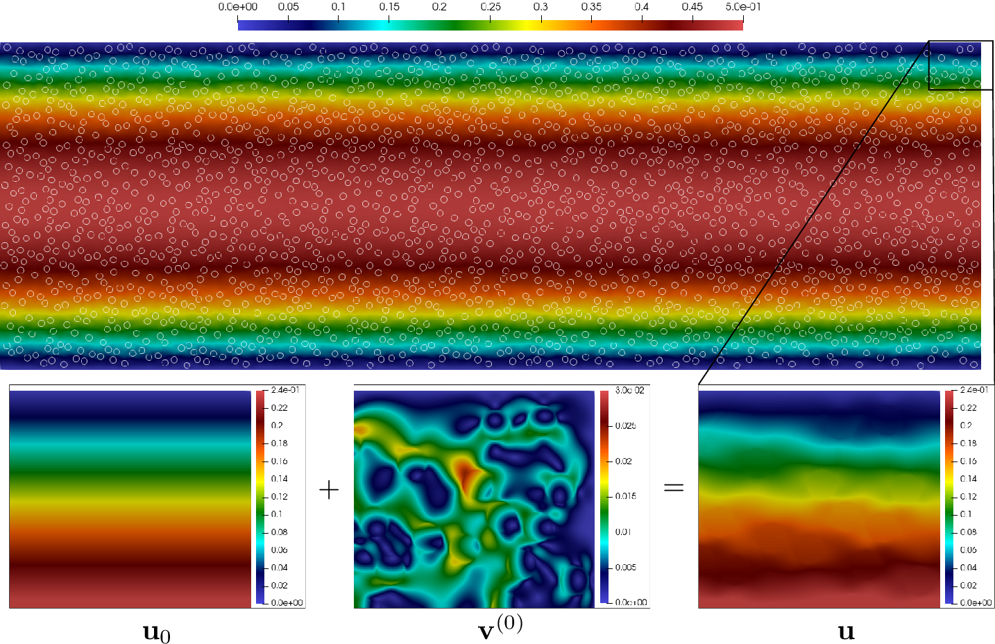
The decomposition of the exact field into a lowest-fidelity field and an error field is illustrated in 2. Identifying an equation governing the lowest-fidelity error is crucial to our approach. Indeed, to improve the approximation quality, a second fidelity level is introduced on top of \((\mathbf{u}_0,p_0)\), based on ?? . More specifically, a two-fidelity approximation of \((\mathbf{u},p)\) will be constructed as \((\mathbf{u}_0+\mathbf{v}_0,p_0+q_0)\), where \((\mathbf{v}_0,q_0)\) approximates the solution \((\mathbf{v}^{(0)},q^{(0)})\) of ?? .
Note that we seek a surrogate \((\mathbf{v}_0,q_0)\) rather than directly computing \((\mathbf{v}^{(0)},q^{(0)})\), since solving ?? incurs essentially the same computational cost as solving the original problem 2 . In particular, both problems are affected by the same computational challenges associated with resolving the droplet interfaces.
2.2 Further fidelities↩︎
As outlined above, in order to recover computational tractability of the error equation ?? , we consider a second auxiliary problem. Only the volume and interface effects of a single droplet are kept, while all other droplets, as well as the domain boundaries, are removed: given a connected \(\Omega_B^i\subset\Omega_B\) (a single droplet), we look at \[\label{eq:singledroplet} \begin{cases} -\nabla\cdot{\boldsymbol{\sigma}}(\mathbf{v},q;\mu)=2(\mu-\mu_F)\nabla\cdot{\boldsymbol{\varepsilon}}(\boldsymbol{\phi}) & \text{in } \Omega_B^i,\\ -\nabla\cdot{\boldsymbol{\sigma}}(\mathbf{v},q;\mu_F)=\mathbf{0}& \text{in } \mathbb{R}^d\setminus\overline{\Omega_B^i},\\ \nabla\cdot\mathbf{v}=0 & \text{in } \mathbb{R}^d\setminus\partial\Omega_B^i,\\ \left\llbracket\mathbf{v}\right\rrbracket=\mathbf{0}& \text{on } \partial\Omega_B^i,\\ \left\llbracket{\boldsymbol{\sigma}}(\mathbf{v},q;\mu)\mathbf{n}\right\rrbracket=\left(\widetilde{\gamma}\kappa\mathrm{I}-2\left\llbracket\mu\right\rrbracket{\boldsymbol{\varepsilon}}(\boldsymbol{\phi})\right)\mathbf{n}& \text{on } \partial\Omega_B^i,\\ \lim_{\left\|\mathbf{x}\right\|\to\infty}\mathbf{v}(\mathbf{x})=\mathbf{0}.& \end{cases}\tag{5}\] The surface tension coefficient \(\widetilde{\gamma}\) and the generic flow field \(\boldsymbol{\phi}\in[H^1(\Omega_B^i)]^d\) are meant as placeholders, although initially equal to \(\gamma\) and \(\mathbf{u}_0\), respectively, cf. 1.
This formulation resembles the full consistency equations in 1, after replacing the correct viscosity field \(\mu\) with \[\label{eq:mupartial} \mu_F+(\mu|_{\Omega_B^i}-\mu_F)\chi_{\Omega_B^i},\tag{6}\] that is, assuming that only the \(i\)-th droplet is present. Here and elsewhere, \(\chi_A\) denotes the indicator function of \(A\), equal to \(1\) on \(A\) and \(0\) elsewhere.
Note that 5 is cast in free \(\mathbb{R}^d\)-space and a zero velocity far-field is imposed for closure. This achieves four beneficial effects:
When, in the original problem 2 , the gap between a droplet \(\Omega_B^i\) and the domain boundary \(\partial\Omega\) is small, one is required to employ highly refined discretizations. See 6 for more details. This issue is completely absent in 5 due to the boundary removal.
If two droplets \(\Omega_B^i\) and \(\Omega_B^{i'}\) are (geometrically) similar to each other, the corresponding problems 5 can be mapped one to the other through simple affine mappings \(\Omega_B^i\mapsto\Omega_B^{i'}\) and changes in \(\widetilde{\gamma}\) and \(\boldsymbol{\phi}\). As discussed in 3.4, this can be exploited for efficiency gains.
Non-homogeneous forcing terms are present only at \(\overline{\Omega_B^i}\) and decay conditions are imposed at infinity, so that the magnitude of the solution \((\mathbf{v},q)\) can be expected to decrease as the distance from the droplet increases. See also 3.3 below. In a fundamental way, this achieves localization in each droplet’s effect on the flow, which is crucial for the convergence of our approach.
Problem 5 naturally lends itself to a boundary-integral-based discretization, where the infinite domain size is actually beneficial rather than detrimental [18]. In particular, approximating the solution to this problem through boundary-integral equations is much simpler than if boundary conditions at \(\partial\Omega\) had been imposed.
3 Surrogate modeling↩︎
In what follows, we restrict our attention to configurations where all \(M\) droplets are circular: \[\Omega_B=\bigcup_{i=1}^M\underbrace{B(\mathbf{x}_i;r_i)}_{\Omega_B^i},\] where centers \(\mathbf{x}_i\) and radii \(r_i\) are suitably chosen so that droplets \(\overline{\Omega_B^i}\) are pairwise disjoint and \(\overline{\Omega_B}\subset\Omega\), in line with our working assumptions. This condition greatly simplifies both the analytical derivations and the construction of surrogate models, while still capturing the essential features of the problem. In 3.5 we discuss possible extensions to non-circular droplets, which might be of particular relevance when simulating time-dependent flows, where interfaces naturally deform.
If all droplets are circular, then the effects of surface tension may be accounted for in an exact way through pressure jumps. Specifically, recalling that surface tension is uniform on each droplet’s boundary but possibly different across droplets, consider \[\widetilde{p}=\sum_{i=1}^M\frac{\gamma_i}{r_i}\chi_{\Omega_B^i},\] where \(\gamma_i:=\gamma|_{\partial \Omega_B^i}\in\mathbb{R}\). Then \((\mathbf{u},p-\widetilde{p})\) satisfies \[\begin{cases} -\nabla\cdot{\boldsymbol{\sigma}}(\mathbf{u},p-\widetilde{p};\mu)=\mathbf{f}& \text{in } \Omega_B \cup \Omega_F,\\ \nabla\cdot\mathbf{u}=0 & \text{in } \Omega_B \cup \Omega_F,\\ \left\llbracket\mathbf{u}\right\rrbracket=\mathbf{0}& \text{on } \Gamma,\\ \left\llbracket{\boldsymbol{\sigma}}(\mathbf{u},p-\widetilde{p};\mu)\mathbf{n}\right\rrbracket=\mathbf{0}& \text{on } \Gamma,\\ \mathbf{u}=\mathbf{g}_D& \text{on } \Gamma_D,\\ {\boldsymbol{\sigma}}(\mathbf{u},p-\widetilde{p};\mu)\mathbf{n}=\mathbf{g}_N& \text{on } \Gamma_N, \end{cases}\] cf. 2 . This is easily seen by linearity of the equation and by inspecting the curvature \(\kappa\equiv r_i^{-1}\) on \(\partial \Omega_B^i\).
For this reason, in describing our surrogate-modeling strategy, we may assume that no surface tension is present without loss of generality: \(\gamma=0\). Indeed, any nonzero amount of surface tension may be accounted for by just adding \(\widetilde{p}\) to the surrogate in a post-processing step.
3.1 Initial correction↩︎
As outlined in 2, we take the solution \((\mathbf{u}_0,p_0)\) of the “no-droplet” Stokes problem 3 with the prescribed boundary data \((\mathbf{g}_D,\mathbf{g}_N)\) as a first low-fidelity surrogate. This solution satisfies all boundary conditions on \(\partial\Omega\) but fails to satisfy the stress balance equation within the droplets \(\Omega_B\) and the interfacial force balance at \(\Gamma=\partial\Omega_B\).
This situation is captured in 1, which shows that, to steer \((\mathbf{u}_0,p_0)\) toward the true solution \((\mathbf{u},p)\) of 2 , one would in principle need to add a globally supported correction \((\mathbf{v}^{(0)},q^{(0)})\) solving ?? . However, computing such correction by solving ?? is computationally unfeasible, since we would require dealing with all droplets’ effects simultaneously. Instead, we construct a computationally cheaper surrogate correction \((\mathbf{v}_0,q_0)\approx(\mathbf{v}^{(0)},q^{(0)})\) via localized corrections.
First, note that the correction equation ?? has non-homogeneous forcing terms supported over \(\overline{\Omega_B}\), which, if \(M\) non-overlapping droplets are present, consists of \(M\) disjoint connected components. The trick to recover tractability is to replace the single problem ?? with forcing terms at \(M\) droplets with \(M\) independent problems, each having forcing terms at a single droplet. More concretely, we consider a collection of \(M\) problems resembling 5 , each targeting a different droplet \(\Omega_B^i\), namely, \[\label{eq:singledropfull} \begin{cases} -\nabla\cdot{\boldsymbol{\sigma}}(\mathbf{v}_{0,i},q_{0,i};\mu)=2(\mu-\mu_F)\nabla\cdot{\boldsymbol{\varepsilon}}(\mathbf{u}_0)&\text{in }\Omega_B^i,\\ -\nabla\cdot{\boldsymbol{\sigma}}(\mathbf{v}_{0,i},q_{0,i};\mu_F)=\mathbf{0}&\text{in }\Omega_B\cup\Omega_F\setminus \Omega_B^i,\\ \nabla\cdot\mathbf{v}_{0,i}=0&\text{in }\Omega_B\cup\Omega_F,\\ \left\llbracket\mathbf{v}_{0,i}\right\rrbracket=\mathbf{0}&\text{on }\Gamma,\\ \left\llbracket{\boldsymbol{\sigma}}(\mathbf{v}_{0,i},q_{0,i};\mu)\mathbf{n}\right\rrbracket=-2\left\llbracket\mu\right\rrbracket{\boldsymbol{\varepsilon}}(\mathbf{u}_0)|_{\Omega_B^i}\mathbf{n}&\text{on }\partial \Omega_B^i,\\ \left\llbracket{\boldsymbol{\sigma}}(\mathbf{v}_{0,i},q_{0,i};\mu_F)\mathbf{n}\right\rrbracket=\mathbf{0}&\text{on }\Gamma\setminus\partial \Omega_B^i, \end{cases}\tag{7}\] for \(i=1,\ldots,M\). Note that, as outlined above, we neglect surface tension (\(\gamma=0\)) since that can be accounted for exactly in the case of circular droplets.
In the above \(M\) problems, we specify no boundary conditions on \(\partial\Omega\). Although 1 assumes homogeneous data there, we instead solve each problem through 5 (setting \(\widetilde{\gamma}=0\) and \(\boldsymbol{\phi}=\mathbf{u}_0\)), where the homogeneous Stokes equation is extended to \(\mathbb{R}^d\setminus \Omega_B^i\) and decay conditions as \(\left\|\mathbf{x}\right\|\to\infty\) are enforced for closure. The benefits of this have been discussed in 2.2.
Remark 2. This decomposition into \(M\) problems with a simply supported forcing term bears some similarity to a partition-of-unity strategy, in that global forcing terms are decomposed into \(M\) local contributions at each droplet.
The first correction is then defined by summing the \(M\) local contributions, \[\mathbf{v}_0=\sum_{i=1}^M\mathbf{v}_{0,i}, \qquad q_0=\sum_{i=1}^Mq_{0,i},\] yielding the updated intermediate approximation \[\mathbf{u}_{1/2}=\mathbf{u}_0+\mathbf{v}_0, \qquad p_{1/2}=p_0+\sum_{i=1}^M\frac{\gamma_i}{r_i}\chi_{\Omega_B^i}+q_0.\] (Note that the surface-tension-related pressure term discussed above has also been included.)
Several further observations are crucial at this point:
Each \((\mathbf{v}_{0,i},q_{0,i})\) is computed based on the modified viscosity field 6 , which is inconsistent with the true \(\mu\) at all droplets except the \(i\)-th one. Consequently, if \(M>1\), \((\mathbf{u}_{1/2},p_{1/2})\) violates the Stokes equations at all droplet locations. This is made rigorous in 3 below. Nevertheless, as we discuss in 3.3, we expect the intermediate approximation \((\mathbf{u}_{1/2},p_{1/2})\) to be more accurate than the lowest-level surrogate \((\mathbf{u}_0,p_0)\) at \(\overline{\Omega_B}\), despite the partial lack of consistency.
The homogeneous boundary conditions at \(\partial\Omega\) are neglected in favor of the more computationally efficient decay conditions as \(\left\|\mathbf{x}\right\|\to\infty\). As such, \((\mathbf{v}_0,q_0)\) has support that includes the whole \(\overline{\Omega}\), so that the new approximation \((\mathbf{u}_{1/2},p_{1/2})\) violates the boundary conditions on \(\partial\Omega\).
These observations behoove us to add further corrections to improve consistency and accuracy. In order to streamline our approach, we choose to follow up the newly added “droplet correction” \((\mathbf{v}_0,q_0)\) with a “boundary correction” \((\mathbf{v}_{1/2},q_{1/2})\), whose target is recovering consistency in the boundary conditions at \(\partial\Omega\).
To derive a boundary-correction equation, we first identify the error in Dirichlet and Neumann boundary conditions: \[\begin{cases} (\mathbf{u}-\mathbf{u}_{1/2})|_{\Gamma_D}=\mathbf{g}_D-(\mathbf{u}_0+\mathbf{v}_0)|_{\Gamma_D}=-\mathbf{v}_0|_{\Gamma_D}=:\widetilde{\mathbf{g}}_{D,1/2},\\ ({\boldsymbol{\sigma}}(\mathbf{u},p;\mu)\mathbf{n}-{\boldsymbol{\sigma}}(\mathbf{u}_{1/2},p_{1/2};\mu)\mathbf{n})|_{\Gamma_N}=\ldots=-({\boldsymbol{\sigma}}(\mathbf{v}_0,q_0;\mu)\mathbf{n})|_{\Gamma_N}=:\widetilde{\mathbf{g}}_{N,1/2}. \end{cases}\] Adding any correction field \((\mathbf{v}_{1/2},q_{1/2})\) satisfying the above boundary conditions would yield a surrogate that is consistent at the domain boundaries. In order to reduce the “interior inconsistencies” that such correction adds, we compute \((\mathbf{v}_{1/2},q_{1/2})\) by solving the no-droplet Stokes problem 3 with uniform viscosity \(\mu_F\), replacing the original boundary conditions \(\mathbf{g}_D\) and \(\mathbf{g}_N\) with \(\widetilde{\mathbf{g}}_{D,1/2}\) and \(\widetilde{\mathbf{g}}_{N,1/2}\), respectively. We then obtain the updated approximation \[\mathbf{u}_1 := \mathbf{u}_{1/2} + \mathbf{v}_{1/2}, \qquad p_1 := p_{1/2} + q_{1/2},\] which, by construction and linearity, satisfies the correct boundary conditions in the original problem 2 , as well as the Stokes equation in the fluid domain \(\Omega_F\) and continuity of the flow field across \(\Gamma\).
3.2 Further corrections and iteration↩︎
Similarly to the lowest-fidelity surrogate \((\mathbf{u}_0,p_0)\), approximation \((\mathbf{u}_1,p_1)\) attains the correct boundary conditions but does not satisfy the stress balance equation within the droplets \(\Omega_B\) nor the interfacial force balance at \(\Gamma=\partial\Omega_B\). At the same time, we expect the updated surrogate to be more accurate, e.g., in the sense that its residual with respect to the original PDE 2 is smaller.
To further improve accuracy, we iterate the above steps, leading to the alternating correction scheme summarized in 3. Termination criteria are discussed in 3.3.
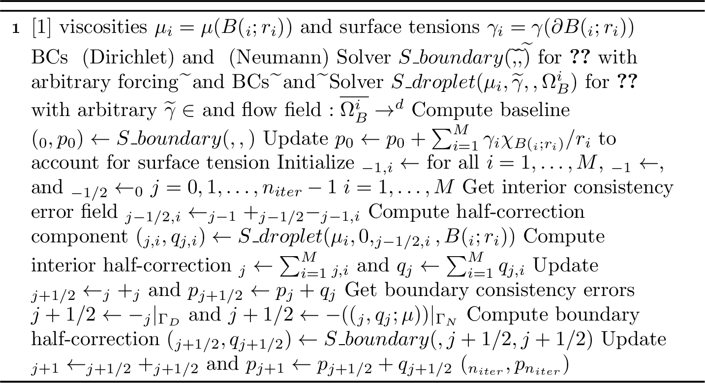
Fundamentally, each iteration proceeds in the same way: \(M\) solves of 5 (one per droplet) are followed by a single global solve of 3 to restore boundary consistency. In particular, at the \(j\)-th iteration of 3, we set up \(M\) different one-droplet error equations 5 with certain forcing terms \(\boldsymbol{\phi}=\boldsymbol{\phi}_{j-1/2,i}\), whose solutions are \((v_{j,i},q_{j,i})\), \(i=1,\ldots,M\). As the following result shows, the forcing terms \(\boldsymbol{\phi}_{j-1/2,i}\) are selected so that the partial correction \((\mathbf{u}_j+\mathbf{v}_{j,i},p_j+q_{j,i})\) is consistent with the original equation over the \(i\)-th droplet (although it is inconsistent at other droplets), generalizing 1.
Proposition 3. For any \(j\ge0\), let \((\mathbf{u}_j,p_j)\) denote the approximation produced by 3. Define the errors \(\mathbf{v}^{(j)}=\mathbf{u}-\mathbf{u}_j\) and \(q^{(j)}=p-p_j\). Then \[\begin{cases} -\nabla\cdot{\boldsymbol{\sigma}}(\mathbf{v}^{(j)},q^{(j)};\mu)=2(\mu-\mu_F)\nabla\cdot{\boldsymbol{\varepsilon}}(\boldsymbol{\phi}_{j-1/2})&\text{in }\Omega_B\cup\Omega_F,\\ \nabla\cdot\mathbf{v}^{(j)}=0&\text{in }\Omega_B\cup\Omega_F,\\ \left\llbracket\mathbf{v}^{(j)}\right\rrbracket=\mathbf{0}&\text{on }\Gamma,\\ \left\llbracket{\boldsymbol{\sigma}}(\mathbf{v}^{(j)},q^{(j)};\mu)\mathbf{n}\right\rrbracket=-2\left\llbracket\mu\right\rrbracket{\boldsymbol{\varepsilon}}(\boldsymbol{\phi}_{j-1/2})|_{\Omega_B}\mathbf{n}&\text{on }\Gamma,\\ \mathbf{v}^{(j)}=\mathbf{0}&\text{on }\Gamma_D,\\ {\boldsymbol{\sigma}}(\mathbf{v}^{(j)},q^{(j)};\mu)\mathbf{n}=\mathbf{0}&\text{on }\Gamma_N, \end{cases}\] where \[\boldsymbol{\phi}_{j-1/2}=\sum_{i=1}^M\sum_{i'\neq i}\mathbf{v}_{j-1,i'}\chi_{\Omega_B^i}+\mathbf{v}_{j-1/2}.\]
Proof. The claim can be shown by induction on \(j\), through careful use of the linearity of problems 2 3 5 . See 6.1 for the full proof. ◻
Remark 4. Note that, for all \(j\) and \(i=1,\ldots,M\), \[\boldsymbol{\phi}_{j-1/2}|_{\Omega_B^i}=\sum_{i'\neq i}\mathbf{v}_{j-1,i'}+\mathbf{v}_{j-1/2}=\mathbf{v}_{j-1}-\mathbf{v}_{j-1,i}+\mathbf{v}_{j-1/2}=\boldsymbol{\phi}_{j-1/2,i},\] justifying line [item:correction] in 3.
As already outlined in 2, the error equation provided in 3 is paramount in our approach, since it gives conditions to be satisfied (in approximate form) by further corrections. We also note the following.
Remark 5. For simplicity, we alternate “droplet corrections” and “boundary corrections”, with each forming a half-step in our iterative procedure. One might consider making several droplet corrections in a row, thus making the process staggered. (Note that repeated boundary corrections would not be useful because full-step surrogates attain boundary consistency.) This option might be useful as a way to achieve a more balanced procedure when droplet errors dominate boundary errors (in some sense). We leave analysis and testing of this option for future work.
Concerning the computational efficiency of 3, it is important to note that the proposed procedure involves repeated solves of 3 and 5 with varying right-hand sides. Especially when these problems are discretized with high resolution, efficiency can be greatly improved by preassembling and pre-factorizing (e.g., via sparse LU) the corresponding stiffness matrices. This is particularly beneficial for 3 . For 5 , an even cheaper approximate strategy can be adopted, potentially avoiding repeated linear solves altogether at the cost of some accuracy. This alternative is discussed in 3.4.
3.3 Convergence considerations↩︎
The iterative scheme of 3 interleaves \(M\) local 5 solvers with a global 3 solver. The problems solved at different iterations differ only in their right-hand sides, i.e., the forcing terms on \(\overline{\Omega_B^i}\) in 5 and the boundary conditions on \(\partial\Omega\) in 3 .
The magnitudes of such right-hand sides, namely, the droplet residual norm \[\label{eq:fixedfull} R_j=\left\|{\boldsymbol{\varepsilon}}(\boldsymbol{\phi}_{j-1/2})\right\|_{L^2(\Omega_B)} + \left\|{\boldsymbol{\varepsilon}}(\boldsymbol{\phi}_{j-1/2})\mathbf{n}\right\|_{H^{-1/2}(\Gamma)}\tag{8}\] at the \(j\)-th “droplet half-step” and the boundary residual norm \[\label{eq:fixedhalf} R_{j+1/2}=\left\|\mathbf{v}_j\right\|_{H^{1/2}(\Gamma_D)} + \left\|{\boldsymbol{\sigma}}(\mathbf{v}_j,q_j;\mu)\mathbf{n}\right\|_{H^{-1/2}(\Gamma_N)}\tag{9}\] at the \(j\)-th “boundary half-step”, \(j=0,1,\ldots\), are useful to study the convergence of the iterates. To more rigorously justify our interest in 8 9 , we note that, by the well-posedness of 3 5, the increment norm \(\left\|\mathbf{u}_{j+1}-\mathbf{u}_j\right\|\) may be bounded in terms of the residual norms, e.g., \[\begin{gather} \left\|\mathbf{u}_{j+1}-\mathbf{u}_j\right\|_{H^1(\Omega\setminus\Gamma)}=\left\|\mathbf{v}_j+\mathbf{v}_{j+1/2}\right\|_{H^1(\Omega\setminus\Gamma)}\leq\sum_{i=1}^M\left\|\mathbf{v}_{j,i}\right\|_{H^1(\Omega\setminus\Gamma)}+\left\|\mathbf{v}_{j+1/2}\right\|_{H^1(\Omega\setminus\Gamma)}\leq\\ \leq C_{\text{1-drop}}\sum_{i=1}^M\big|\mu(\mathbf{x}_i)-\mu_F\big|\left(\left\|{\boldsymbol{\varepsilon}}(\boldsymbol{\phi}_{j-1/2})\right\|_{L^2(\Omega_B^i)} + \left\|{\boldsymbol{\varepsilon}}(\boldsymbol{\phi}_{j-1/2})\mathbf{n}\right\|_{H^{-1/2}(\partial\Omega_B^i)}\right)+C_{\text{0-drop}}R_{j+1/2}\leq\\ \leq\widetilde{C}_{\text{1-drop}}\max_i\big|\mu(\mathbf{x}_i)-\mu_F\big|R_j+C_{\text{0-drop}}R_{j+1/2}. \end{gather}\] A similar derivation holds for the pressure increment \(\left\|p_{j+1}-p_j\right\|=\left\|q_j+q_{j+1/2}\right\|\).
Although further work is needed to fully analyze the convergence of the residual norms, we outline here an intuitive reason why we expect the residuals to decrease as \(j\to\infty\). At iteration \(j\), the correction \((\mathbf{v}_{j,i},q_{j,i})\) due to the \(i\)-th droplet affects the boundary residual norm \(R_{j+1/2}\) only through boundary evaluations \(\mathbf{v}_{j,i}|_{\Gamma_D}\) and \({\boldsymbol{\sigma}}(\mathbf{v}_{j,i},q_{j,i};\mu)\mathbf{n}|_{\Gamma_N}\). As displayed, e.g., in 4, we have empirical evidence that local corrections \((\mathbf{v}_{j,i},q_{j,i})\) decay away from the \(i\)-th droplet, i.e., that the surrogate correction fields are “smaller” on the domain boundary than on the droplets that cause them. As such, field decay heuristically suggests that \(R_{j+1/2}\lesssim R_j\).
On the other hand, we may heuristically assume that \(R_{j+1}\lesssim R_{j+1/2}\) since boundary corrections at iteration \(j\) affect field \(\boldsymbol{\phi}_{j+1/2}\) at iteration \((j+1)\) through the well-posed no-droplets Stokes equation 3 . Unfortunately, this argument is not rigorous, since we have no theoretical handle on the constants involved in the above inequalities, especially because the Stokes equation is not endowed with an elliptic “maximum principle”.
Remark 6. By the above argument, we expect the convergence rate to suffer if a droplet is near the domain boundary, or even if two droplets are particularly close to each other. While this should ultimately be subject to a thorough theoretical analysis, we include some tests on the performance of our method in such regimes in 5. As a way to partially counteract the slow convergence due to such small gaps, we believe that it should be possible to design specialized correction problems that replace the single droplet in 5 with a (small) droplet cluster. We leave this as a direction for future research.
At the same time, we note that such settings are difficult to handle even more so with standard approximation techniques. For instance, finite-element-based approaches require mesh refinements, whereas boundary-integral formulations must see a local increase in the number of quadrature points. We expect our approach to deal with such cases (through iteration) more effectively than alternative options do (through refinement).
On the practical side, we require a convergence indicator as stopping criterion in 3. For this we employ a simplified version of the boundary residual 9 , with the \(L^\infty\)-norm replacing the expensive \(H^{\pm1/2}\) ones. This is cheaply computable and readily available, since evaluations of the boundary residual are anyway needed when solving 3 within 3. More robust, but costly, alternative termination criteria may also be based on global \(L^2(\Omega)\)- or \(H^1(\Omega)\)-norms of the full increments \(\mathbf{u}_{j+1}-\mathbf{u}_j=\mathbf{v}_j+\mathbf{v}_{j+1/2}\).
Remark 7. If the chosen convergence indicator provides evidence of diverging behavior, it remains possible to introduce a relaxation parameter \(0<\omega<1\), as is typical in iterative (e.g., Richardson) schemes [19]. In 3, a Richardson relaxation can be achieved through a simple rescaling5 of all fields \(\boldsymbol{\phi}_{j,i}\) by the factor \(\omega\). While potentially improving the methods’ stability, this strategy may obviously lead to reduced convergence speeds if \(\omega\) is chosen too small. In our numerical experiments in 5, relaxation was never needed.
3.4 Improving efficiency by exploiting self-similarity↩︎
We now discuss how to accelerate the computation of single-droplet problems 5 in free space. This is crucial for speeding up calculations in 3, since the single-droplet problem must be solved \(M\) times within each iteration. In the approach described below, we rely on the fact that droplets are geometrically similar to each other, i.e., that affine transformations exist mapping each droplet to any other. Since we are presently working under the assumption that droplets are circular, this is obviously true. Extensions to non-circular droplets, as might arise in time-dependent simulations, are discussed in 3.5. In addition, we will assume that the surface tension is \(\widetilde{\gamma}=0\) for simplicity (as discussed at the beginning of 3, this assumption is natural for circular droplets), although our presentation naturally generalizes to non-trivial surface tensions.
By geometric similarity of the droplets, the \(M\) single-droplet problems 5 (one per droplet) may be remapped to a reference configuration, viz., the unit disk \(\Omega_B^\sharp=B(\mathbf{0};1)\), through droplet-dependent affine mappings. See 6.2 for more details and refer to 2.2 for a discussion on how this follows from our choice of an unbounded domain. As such, the task of (approximately) solving 5 on \(M\) different domains and forcing terms can then be replaced by the task of solving 5 on the unit disk with the \(M\) different forcing terms resulting from the remappings. Equivalently, we must evaluate operator \[\begin{align} \mathcal{S}:[H^1(\Omega_B^\sharp)]^d&\to[H^1(\mathbb{R}^d)]^d\times L^2(\mathbb{R}^d)\label{eq:calS}\\ \boldsymbol{\phi}&\mapsto(\mathbf{u},p)\text{ solving \ref{eq:singledroplet} with \Omega_B^i=\Omega_B^\sharp and flow field \boldsymbol{\phi}}\nonumber \end{align}\tag{10}\] at \(M\) different inputs \(\{\widetilde{\boldsymbol{\phi}}_{j-1/2,i}\}_{i=1}^M\) (each obtained by remapping \(\boldsymbol{\phi}_{j-1/2,i}\) from 3), one per droplet, at each iteration.
Remark 8. Operator \(\mathcal{S}\) depends also on the viscosity values \(\mu(\mathbf{x}_i)\) and \(\mu_F\), although this dependence is kept implicit in our notation. This fact is of relevance if different droplets have different viscosities. In such case, the upcoming construction must be repeated for each viscosity value.
A cheap-to-evaluate surrogate for \(\mathcal{S}\) can be built through a (linear) subspace approach: given a set of \(N\) linearly independent vectors \(\{\widehat\boldsymbol{\phi}_k\}_{k=1}^N\subset[H^1(\Omega_B^\sharp)]^d\), for any \(\boldsymbol{\phi}\in[H^1(\Omega_B^\sharp)]^d\) we approximate \(\mathcal{S}(\boldsymbol{\phi})\approx\mathcal{S}(\mathcal{P}_N\boldsymbol{\phi})\), with \(\mathcal{P}_N:[H^1(\Omega_B^\sharp)]^d\to\text{span}\{\widehat\boldsymbol{\phi}_k\}_{k=1}^N\) a suitable projector operator.
Computational efficiency can be achieved by exploiting the linearity of \(\mathcal{S}\). Indeed, introducing the coordinate map \(\mathcal{Q}_N:[H^1(\Omega_B^\sharp)]^d\to\mathbb{R}^N\), defined as \(\sum_{k=1}^N(\mathcal{Q}_N\boldsymbol{\phi})_k\widehat\boldsymbol{\phi}_k:=\mathcal{P}_N\boldsymbol{\phi}\), as well as the fundamental solutions \(\{\mathcal{S}(\widehat\boldsymbol{\phi}_k)\}_{k=1}^N\), we have \[\label{eq:basiss} \boldsymbol{\phi}\approx\mathcal{P}_N\boldsymbol{\phi}=\sum_{k=1}^N(\mathcal{Q}_N\boldsymbol{\phi})_k\widehat\boldsymbol{\phi}_k\quad\Rightarrow\quad\mathcal{S}(\boldsymbol{\phi})\approx\mathcal{S}_N(\boldsymbol{\phi}):=\mathcal{S}(\mathcal{P}_N\boldsymbol{\phi})=\sum_{k=1}^N(\mathcal{Q}_N\boldsymbol{\phi})_k\mathcal{S}(\widehat\boldsymbol{\phi}_k).\tag{11}\] This means that, after precomputing the fundamental solutions, evaluating \(\mathcal{S}_N(\boldsymbol{\phi})\) comes at the only cost of evaluating the coordinate map \(\mathcal{Q}_N\) and a linear combination of fundamental solutions.
Remark 9. In practice, we choose the sampled flow fields \(\{\widehat\boldsymbol{\phi}_k\}_{k=1}^N\) to have polynomial components up to a prescribed degree \(D\geq0\). This has the advantage of implementation simplicity, as well as the guarantee of spectral approximation convergence for spatially smooth fields \(\boldsymbol{\phi}\), although alternatives may be considered. Moreover, it allows evaluating the projector \(\mathcal{P}_N\) and the coordinate map \(\mathcal{Q}_N\) through simple (least-squares) polynomial interpolation. More details on this are provided in 6.3 for \(d=2\) dimensions.
This strategy employs an offline-online decomposition: a large(r) cost is incurred in some precomputation so that later numerical operations may be made cheap(er). Namely, let \(c_{\text{high-fi}}\) denote the cost of a single high-fidelity evaluation of \(\mathcal{S}\) through CutFEM or boundary-integral-based method, and assume that evaluating \(\mathcal{S}_N\) has \(\mathcal{O}(N^3)\ll c_{\text{high-fi}}\) cost because of the coordinate map \(\mathcal{Q}_N\). If \(N_{\text{eval}}\) evaluations of \(\mathcal{S}\) at different inputs are required, then an \(\mathcal{O}(N_{\text{eval}}c_{\text{high-fi}})\) direct-evaluation cost is replaced by an \(\mathcal{O}(Nc_{\text{high-fi}}+N_{\text{eval}}N^3)\) approximate-evaluation cost.

Of course, an error is incurred due to the truncation of the basis at index \(N<\infty\). It is relatively straightforward to derive a priori bounds on the basis-truncation error. Specifically, since 5 is well-posed [20], [21], we can find a \(\boldsymbol{\phi}\)-independent constant \(C\) such that \[\begin{gather} \left\|\mathcal{S}(\boldsymbol{\phi})-\mathcal{S}_N(\boldsymbol{\phi})\right\|_{[H^1_0(\mathbb{R}^d\setminus\partial \Omega_B^\sharp)]^d\times[L^2(\mathbb{R}^d)\setminus\mathbb{R}]}\leq\\ \leq C\big|\mu(\mathbf{0})-\mu_F\big|\left(\left\|{\boldsymbol{\varepsilon}}(\boldsymbol{\phi}-\boldsymbol{\phi}_N)\right\|_{L^2(\Omega_B^\sharp)} + \left\|{\boldsymbol{\varepsilon}}(\boldsymbol{\phi}-\boldsymbol{\phi}_N)\mathbf{n}\right\|_{H^{1/2}(\partial \Omega_B^\sharp)}\right). \end{gather}\] by linearity of \(\mathcal{S}\). As such, we can control the error in the approximation of \(\mathcal{S}(\boldsymbol{\phi})\) by lowering the subspace-projection error. In our experiments, we found that a small \(N\lesssim10\) is enough to achieve good accuracy in \(d=2\) dimensions. Since, in 3, \(N_{\text{eval}}=n_{\text{iter}}M\) may much larger than such \(N\), our approach is justified.
As a final point, we wish to comment on how one may precompute the \(N\) fundamental solutions, corresponding to setting \(\boldsymbol{\phi}=\widehat\boldsymbol{\phi}_k\) in 5 for \(k=1,\ldots,N\). In our numerical tests, we compute these through a boundary-integral formulation, which is natural due to the unboundedness of the domain. Alternatively, finite-elements or finite-differences techniques on truncated domains might also be suitable. In 4 we display some sample fundamental solutions corresponding to the polynomial basis derived in 6.3.
3.5 Extensions↩︎
As discussed in 3.4, an efficient solve of 5 within 3 assumes geometric similarity between each droplet and the reference configuration (the unit disk). This assumption allows a speed-up in each call to \(\text{S\_droplet}\) from approximately \(\mathcal{O}(N_{\text{BIE}}^3)\), with \(N_{\text{BIE}}\) being the number of degrees of freedom used to discretize 5 by boundary-integral equations, cf. 11, to \(\mathcal{O}(N^3)\), with \(N\) the number of fundamental solutions used in 11 . However, droplets may generally differ in shape, for instance and notably, within a time-domain simulation 1 . This requires modifications to the strategy described so far.
Firstly, the assumption of circular droplets allows drastic simplifications in the handling of surface tension, cf. 3. If droplets have general shapes, no analytic correction exists to account for surface tension. As such, surface tension remains part of the interface force balance that is corrected through iteration: a nonzero \(\widetilde{\gamma}\) must be included in 5 . Iterated correction of the surface tension term can be handled within the call to S_droplet, along with the other volume and interface correction terms.
Secondly, and more importantly for computation, our efficient approach from 3.4 cannot be applied if drops are not self-similar. We suggest here three possible options for dealing with this.
3.5.0.1 Rigid-droplet approximation.
Droplet deformations can be neglected at the cost of accuracy. In this setting, each time step induces an easy-to-handle, rigid-body motion of each droplet. This idea is described in 4.2 for circular droplets.
3.5.0.2 Direct computation.
One can skip the idea from 3.4 altogether, directly casting and solving 5 on each droplet without remapping. This incurs the above-mentioned \(\mathcal{O}(N_{\text{BIE}}^3)\) cost per droplet, per iteration. Since a moderate number of degrees of freedom \(N_{\text{BIE}}\) may be needed for a sufficiently accurate representation of the solution \((\mathbf{v},q)\) of 5 , this strategy can incur significant cost.
3.5.0.3 Shape parametrization.
Depending on the application, it might be possible to predict in which ways the droplets will deform, allowing one to design a parametrized family of shapes that the droplets are “allowed” to take [22], [23]. In this setting, the collection of fundamental solutions corresponding to such shapes becomes parameter-dependent too. Cheaply approximating the fundamental solutions induced by an arbitrary parameter choice (i.e., a given droplet shape) may be feasible through interpolation or machine-learning techniques [15], [22] starting from a discrete database of fundamental solutions, obtained by “sampling” the parametrized family of shapes. We leave this extension as future work.
4 Complexity and suggested computational pipelines↩︎
We now discuss the computational complexity of the proposed surrogate model, both at training and evaluation time. Let \(M\) denote the number of droplets and \(N\) the number of fundamental solutions used to approximate the action of the single-droplet solution operator \(\mathcal{S}\) in 11 . To streamline our discussion, we will assume that \(M>N\), since (i) our numerical tests show that a small number \(N\) of fundamental solutions is usually sufficient to achieve modest accuracy (say, \(10^{-4}\)), cf. the theoretical discussion in 3.4 as well as our numerical tests in 5, and (ii) the many-droplet regime is ultimately our target.
We specialize our discussion to two useful computational pipelines that use 3 11 to emulate 2 . They apply in different scenarios, depending on the target application.
4.1 Pipeline 1: static emulation of the solution field↩︎
A first setting where our surrogate model is useful is when one aims to approximately compute the stationary solution of the Stokes interface problem 2 . This is relevant, for instance, when investigating the effect of the droplets \(\Omega_B\) on the surrounding flow field. In this context, one may wish to evaluate \((\mathbf{u},p)\) at a collection of \(n_{\text{eval}}\) points in \(\Omega\), e.g., for visualization or postprocessing purposes. To this end, it suffices to execute 3 with 11 and subsequently evaluate the resulting surrogate at the desired target points. The overall computational complexity of this procedure can be derived as follows.
We first ignore the training procedure (the loop in 3) and focus only on the evaluation task. If \(n_{\text{iter}}\) iterations are carried out within 3, the surrogate is the sum of \((2n_{\text{iter}}+1)\) terms: the surrogate flow field is \[\widetilde{\mathbf{u}}=\underbrace{\mathbf{u}_0+\mathbf{v}_{1/2}+\ldots+\mathbf{v}_{n_{\text{iter}}-1/2}}_{\widetilde{\mathbf{u}}_{\text{boundary}}}+\underbrace{\mathbf{v}_0+\ldots+\mathbf{v}_{n_{\text{iter}}-1}}_{\widetilde{\mathbf{u}}_{\text{droplets}}}.\] The surrogate pressure field has a similar expansion, which we ignore for simplicity in the following.
Note that, above, we have grouped together all half-step corrections with the baseline solution \(\mathbf{u}_0\) into \(\widetilde{\mathbf{u}}_{\text{boundary}}\), since all \((n_{\text{iter}}+1)\) addends relate to global Stokes solutions computed via \(\text{S\_boundary}\), whose purpose is enforcing the boundary conditions on \(\partial\Omega\), disregarding droplets. In a computational framework, we may assume that all such field have been computed using the same (e.g., FEM-based) discretization of 3 (with different boundary conditions). By linearity, we may thus add all contributions together into a single “vector of degrees of freedom”, so that evaluating \(\widetilde{\mathbf{u}}_{\text{boundary}}\) has \(n_{\text{iter}}\)-independent evaluation cost \(c_{\text{boundary}}\).
By a similar token, we can exploit the similarity between all terms adding up to \(\widetilde{\mathbf{u}}_{\text{droplets}}\). Namely, we can express \[\mathbf{v}_j=\sum_{i=1}^M\sum_{k=1}^N\alpha_{i,j,k}\widehat\mathbf{v}_k\circ\eta_i\] where \(M\) is the number of droplets, \(\eta_i\) are the affine mappings defined in 3, and \(\alpha_{i,j,k}\) are the fundamental-solution-expansion coefficients \((\mathcal{Q}_N\boldsymbol{\phi}_{j-1/2,i})_k\), cf. 11 . From here, we can compute \[\label{eq:surrdroplet} \widetilde{\mathbf{u}}_{\text{droplets}}=\sum_{j=0}^{n_{\text{iter}}-1}\sum_{i=1}^M\sum_{k=1}^N\alpha_{i,j,k}\widehat\mathbf{v}_k\circ\eta_i=\sum_{i=1}^M\underbrace{\left(\sum_{j=0}^{n_{\text{iter}}-1}\sum_{k=1}^N\alpha_{i,j,k}\widehat\mathbf{v}_k\right)\circ\eta_i}_{\widetilde{\mathbf{v}}_i:=}.\tag{12}\] Both indices \(j\) and \(k\) in the above expression can be collapsed, which leads to precomputing the \(M\) fields \(\widetilde{\mathbf{v}}_i\), each corresponding to the total effect that a droplet has on the field. In this way, we can make the cost of evaluating \(\widetilde{\mathbf{u}}_{\text{droplets}}\) independent of \(N\) and \(n_{\text{iter}}\).
On the other hand, it is not computationally possible to achieve an accurate representation of \(\widetilde{\mathbf{u}}_{\text{droplets}}\) without incurring an \(\mathcal{O}(M)\) scaling, e.g., by collapsing the “droplet index” \(i\) in 12 . Indeed, each droplet contributes to the total solution with a field that displays very localized features around the droplet itself, cf. our numerical results below. An accurate numerical representation of the total field \(\widetilde{\mathbf{u}}_{\text{droplets}}\) must thus necessarily resolve such effects, resulting in a linear scaling in \(M\).
In summary, the cost of a single surrogate evaluation scales as \(\mathcal{O}(Mc_{\text{droplet}}+c_{\text{boundary}})\), with \(c_{\text{droplet}}\) being the \(n_{\text{iter}}\)- and \(N\)-independent cost of evaluating each of the fields \(\widetilde{\mathbf{v}}_i\) in 12 at a single point.
Remark 10. In several settings, e.g., if many droplets are present (\(M\gg1\)) or if 3 is discretized on a coarse mesh, the cost \(c_{\text{boundary}}\) is negligible. In this regime, which we assume for simplicity from now on, the total cost of a single surrogate evaluation scales linearly with \(M\).
We now go back to the training procedure, consisting of an iterative correction loop. At the \(j\)-th iteration, the dominant costs arise from four sources:
Assembling the flow field \(\boldsymbol{\phi}_{j-1/2,i}\) for each droplet \(i=1,\ldots,M\). Since this requires evaluating the current surrogate, cf. the definition of \(\boldsymbol{\phi}_{j-1/2,i}\), this has asymptotic cost \(\mathcal{O}(M^2c_{\text{droplet}})\), cf. 10.
Solving 5 to find the volume corrections \((\mathbf{v}_{j,i},q_{j,i})\) for each droplet \(i=1,\ldots,M\). Assuming that 11 is used and that the basis-expansion coefficients \(\alpha_{i,j,k}\) are computed by interpolation, we can expect an \(\mathcal{O}(M^2Nc_{\text{droplet}}+MN^3)\) cost, due to having to evaluate each \(\boldsymbol{\phi}\) at \(N\) points and solve \(M\) size-\(N\) interpolation problems. The complexity can be simplified to \(\mathcal{O}(M^2Nc_{\text{droplet}})\) if \(M\gg N\).
Assembling and evaluating the boundary errors \(\widetilde{\mathbf{g}}_{D,j+1/2}\) and \(\widetilde{\mathbf{g}}_{N,j+1/2}\) at \(\Gamma_D\) and \(\Gamma_N\), respectively. Assuming that \(n_{\text{BC}}\) boundary evaluations are needed in order for \((\mathbf{u}_{j+1/2},q_{j+1/2})\) to be then computed through \(\text{S\_boundary}\), this costs \(\mathcal{O}(Mc_{\text{droplet}}n_{\text{BC}})\).
Solving 3 within \(\text{S\_boundary}\) to find \((\mathbf{u}_{j+1/2},q_{j+1/2})\). We denote the corresponding cost by \(c_{\text{Stokes}}\).
In the setting described in 10, the second step has the largest complexity. Notably, the last step has especially low cost \(c_{\text{Stokes}}\) if the matrix associated with the discretization of 3 is pre-factorized as suggested in 3.2. In such cases, the training complexity scales as \(\mathcal{O}(M^2Nc_{\text{droplet}}n_{\text{iter}})\) overall.
Remark 11. More generally, the cost of the most expensive step ([step:exp] above) depends on the specific strategy used to obtain \((\mathbf{v}_{j,i},q_{j,i})\). For instance, computing such fields “on the fly” by boundary-integral equations, discretized using \(N_{\mathrm{BIE}}\) degrees of freedom, costs approximately \(\mathcal{O}(M^2N_{\mathrm{BIE}}c_{\mathrm{droplet}}+MN_{\mathrm{BIE}}^3)\).
Putting all together yields a complexity of \[\mathcal{O}\left(M\big(MNn_{\text{iter}} + n_{\text{eval}}\big)c_{\text{droplet}}\right).\] In our experiments, we have observed that, in some cases, the cost of the evaluation phase may dominate, especially when \(n_{\text{eval}}\) is large. This can occur, for example, when targeting high-resolution visualizations of the solution field. Concerning this, it is worth noting that surrogate evaluations are “embarassingly parallelizable”, which may allow for substantial speedups in practice.
Remark 12. The quadratic scaling in \(M\) is a symptom of the pairwise interactions between droplets during training. It might be possible to accelerate the training, reducing its complexity to \(M\log M\), through spatially hierarchical strategies in the style of the fast multipole method [24]. To achieve this, one leverages the decay of the interaction forces (here, the fundamental solutions \(\{\mathcal{S}(\widehat\boldsymbol{\phi}_k)\}_k\)) as the distance between droplets increases to replace exact one-to-one interactions between distant droplets with approximate many-to-many interactions. Work on this idea is under way.
4.2 Pipeline 2: time-domain simulation of moving droplets↩︎
A second setting with practical relevance is that where the positions and shapes of the droplets \(\Omega_B\) vary with time, since droplets are advected and deformed by the flow field solving 2 . More rigorously, we consider the time-dependent problem 1 .
To handle this problem efficiently, we propose a surrogate-based evolution strategy. The key idea is to decouple the geometric evolution from the fluid solve by leveraging the surrogate model to rapidly evaluate the local velocity field acting on each droplet. At each time step \(t_n\) in a time grid6 \(0=t_0<t_1<\ldots<t_{N_{\text{time}}}\), the following procedure is carried out:
Given the current droplet configuration \(\Gamma(t_n)\), use 3 to evaluate the surrogate model to obtain the approximate velocity field \(\widetilde{\mathbf{u}}(t_n)\).
Place \(n_{\text{adv}}\) “markers” on each droplet (e.g., uniformly spaced on its boundary) \(\{\mathbf{x}_{l,i}(t_n)\}_{l=1}^{n_{\text{adv}}}\subset\Gamma_i(t_n)\) for \(i=1,\ldots,M\). Evaluate \(\widetilde{\mathbf{u}}(t_n)\) there.
Update droplet positions and shapes by a forward-Euler step over all droplets’ boundaries: \[\mathbf{x}_{l,i}(t_{n+1})=\mathbf{x}_{l,i}(t_n)+(t_{n+1}-t_n)\widetilde{\mathbf{u}}(t_n)|_{\mathbf{x}_{l,i}(t_n)}.\]
Update \(n\gets n+1\) and go to step [item:step].
This approach allows the flow–structure coupling to be approximated without solving a full Stokes system at every time step.
It is crucial to observe that the above strategy will generally result in substantial deformations in the droplets’ shapes, since the markers \(\{\mathbf{x}_{l,i}\}_{l=1,i=1}^{n_{\text{adv}},M}\) are advected independently. This ultimately may result in unstable behavior, requiring the use of relaxation strategies [15]. Moreover, as our methods have been so far developed for circular droplets, we cannot yet handle general shape deformations. We refer to 3.5 for discussion on that.
To recover tractability, we suggest a simplified advection strategy, which shifts each droplet by a rigid translation by averaging the corresponding markers’ velocities: \[\label{eq:timestep95markers} \mathbf{x}_{l,i}(t_{n+1})=\mathbf{x}_{l,i}(t_n)+(t_{n+1}-t_n)\frac{1}{n_{\text{adv}}}\sum_{l'=1}^{n_{\text{adv}}}\widetilde{\mathbf{u}}(t_n)|_{\mathbf{x}_{l',i}(t)}.\tag{13}\] This formula preserves droplet shapes at the cost of accuracy, especially when droplets deform substantially as a result of interactions with nearby droplets or boundaries. The computational cost of the resulting time-domain simulation scales as \(\mathcal{O}(M^2(Nn_{\text{iter}} + n_{\text{adv}})c_{\text{droplet}}N_{\text{time}})\).
5 Numerical examples↩︎
We perform a suite of numerical tests to validate the accuracy and efficiency of the proposed method for multiphase Stokes problems in \(d=2\) spatial dimensions. We consider a viscosity contrast of \(100\), with piecewise-constant viscosity \(\mu=\mu_F=1\) outside the droplets and \(\mu=100\) inside them. We set the volume forcing \(\mathbf{f}=\mathbf{0}\) and the surface tension coefficient \(\gamma=10\). Unless otherwise specified, we employ the following surrogate setup:
We use 3, stopping the fixed-point iterations, indexed by \(j\), according to the criterion \[\label{eq:fixedhalflinf} \left\|\mathbf{v}_j\right\|_{L^\infty(\Gamma_D)} + \left\|{\boldsymbol{\sigma}}(\mathbf{v}_j,q_j;\mu)\right\|_{L^\infty(\Gamma_N)}\leq\mathrm{tol}=10^{-3},\tag{14}\] cf. 3.3. This choice of \(\mathrm{tol}\) is validated in our first test.
We use 11 to more efficiently solve the single-droplet auxiliary problem 5 . Namely, the flow field \(\boldsymbol{\phi}\) is approximated through a polynomial of degree \(D=2\), which results in \(N=6\) fundamental solutions, cf. [sec:basis] [app:poly]. The subspace projection \(\boldsymbol{\phi}\mapsto\boldsymbol{\phi}_N\) is carried out via least-squares interpolation using \(8D\) uniformly distributed points on \(\Omega_B^i\), which is intended to mimic \(L^2(\Omega_B^i)\)-projection by quadrature. This choice of \(D\) is validated in our first test.
The lowest-fidelity solution \((\mathbf{u}_0,p_0)\) is computed by the finite-element method (FEM) on a relatively coarse grid. The same method is used also to solve 3 through \(\text{S\_boundary}\) within 3. For the sake of efficiency, a sparse LU factorization of the FEM matrix is precomputed and stored to disk.
To test accuracy, we compute reference solutions using CutFEM [6] using the setup described in [25]. For the numerical representation of the interfaces, we use the level-set method [26], [27], where the scalar function \(\phi=\phi(\mathbf{x})\) is used to characterize the droplets region \(\Omega_B:=\{\mathbf{x}\in\Omega:\phi(\mathbf{x})>0\}\) and to discretize 2 using CutFEM, cf. 6.4. The approximation error is computed on the velocity field in the \(L^2(\Omega)\) and \(L^\infty(\Omega)\) norms.
Unless otherwise specified, we run out tests in Python 3.12 on a workstation with an Intel® Core Ultra 7 processor 265 and \(64\)GB of RAM. FEM and CutFEM are implemented in C++ as part of the open-source CutFEM library [28].
Reproducibility code is available at https://github.com/CutFEM/hierarchical2DDropletStokes.
5.1 Convergence test↩︎
We first study the accuracy of our method by looking at the approximation error in the flow field \(\mathbf{u}^{(n_{\mathrm{iter}})}-\mathbf{u}\). We consider a 2D square domain modeling a simple right-angle pipe junction: homogeneous Dirichlet conditions are imposed on the bottom and right boundaries, whereas two parabolic flow profiles (one in-going, one out-going) are imposed on the top and left boundaries through Dirichlet condition.

We consider two droplets (\(M=2\)) with radii \(r_1=0.1\) and \(r_2=0.05\), centered at \(\mathbf{x}_1=(0.3,0.7)\) and \(\mathbf{x}_2=(0.65,0.7)\). We first study how the approximation error changes when varying (i) the approximation degree \(D\) used to approximate 5 with 11 and (ii) the tolerance \(\mathrm{tol}\) set on the boundary residual norm 14 , used to stop the fixed-point iterations in 3. Recall that the numbers of fundamental solutions \(N\) needed for degree \(D\) are \(N=0\) for \(D=0\) and \(N=4D-2\) for \(D>0\).
The number of fixed-point iterations increases as \(\mathrm{tol}\) decreases: tolerances \(10^{-1}\), \(10^{-2}\), and \(10^{-3}\) require \(1\), \(3\), and \(5\) iterations, respectively. The number of fixed-point iterations may generally depend on \(D\) although no variations were observed here. The relative approximation errors are shown in 5 (middle and right). First, we note that the approximation error using just lowest-degree fundamental solutions (\(D=1\)) is already about one order of magnitude lower than that achieved by the lowest-fidelity solution \((\mathbf{u}_0,p_0)\), which corresponds to \(D=0\).
An early termination of the fixed-point iterations due to a too large \(\mathrm{tol}\) leads to saturation with respect to the polynomial degree \(D\). Indeed, despite the more accurate approximation of the local volume residual on the droplet, cf. 3.4, large residuals are left when the fixed-point iterations end. Focusing now on the smallest tested value of \(\mathrm{tol}\), we observe exponential convergence with respect to \(D\) for both \(L^2\) and \(L^\infty\) errors. This is expected since we are performing a spectral (truncated-Taylor) approximation of a smooth function, namely, the flow field \(\boldsymbol{\phi}\) that is given as input to the linear operator \(\mathcal{S}\), cf. 3.4.
As a test to investigate the convergence behavior of the fixed-point iterations with respect to the geometric configuration of the droplets, we fix \(D\) and place the droplets at different distances from the domain boundaries and from each other. See 5 (left). More specifically, given \(\delta\) and \(\epsilon\), we place the droplets’ centers at \(\mathbf{x}_1=(\delta+0.1,0.7)\) and \(\mathbf{x}_2=(\delta+\epsilon+0.25,0.7)\), keeping the radii fixed. This places the first droplet at distance \(\delta\) from the left boundary and the two droplets at distance \(\epsilon\) from each other, cf. 5 (left).
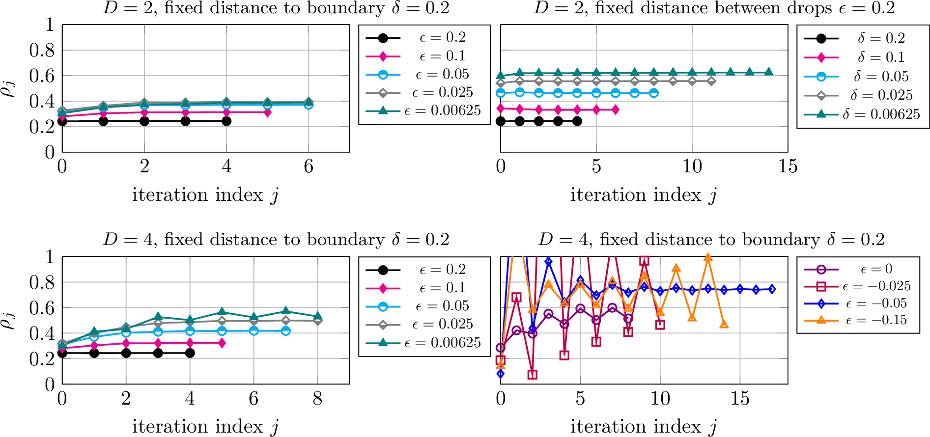
We choose a small \(\mathrm{tol}=10^{-4}\), which results in more iterations than above, in order to allow the convergence behavior to fully develop, leading to a more clear comparison of different values of \(\delta\) and \(\epsilon\). We run 3 to build a surrogate model for each configuration, keeping track of the contraction rate \[\rho_j=\frac{\left\|\mathbf{v}_{j+1}\right\|_{L^\infty(\Gamma_D)} + \left\|{\boldsymbol{\sigma}}(\mathbf{v}_{j+1},q_{j+1};\mu)\right\|_{L^\infty(\Gamma_N)}}{\left\|\mathbf{v}_j\right\|_{L^\infty(\Gamma_D)} + \left\|{\boldsymbol{\sigma}}(\mathbf{v}_j,q_j;\mu)\right\|_{L^\infty(\Gamma_N)}}.\] This provides us with information on the contractive properties of the fixed-point operator and, by proxy, on the convergence properties of the fixed-point loop: larger values of \(\rho_j\) indicate slower convergence, with \(\rho_j\geq1\) being a symptom of no convergence at all. The contraction rate is plotted in 6 for four different configurations and varying values of \(\delta\) and \(\epsilon\). Convergence was reached in all cases. We can make the following remarks:
The top two plots allow us to compare the effects of the distance \(\delta\) between droplets and boundaries versus the distance \(\epsilon\) between droplets only, since one of the two distances is kept fixed while the other varies. Decreasing either \(\delta\) or \(\epsilon\) increases the contraction rate, causing the need for more iterations, cf. 6. However, a small distance \(\delta\) to the domain boundary seems to have a stronger effect on convergence than a small distance \(\epsilon\) between droplets, suggesting that “hard” boundaries hinder our method more than “soft” interfaces.
The left two plots allow us to compare the effects of the truncation degree \(D\) on convergence. We observe that nearby droplets seem to slow convergence down slightly more for larger degrees \(D\). This is likely related to conditioning issues in iterating over the coefficients of higher-degree fundamental solutions. We also observe slight oscillations developing in \(\rho_j\) for \(D=4\) and \(\epsilon=0.00625\). These arise as symptoms of the strong two-way interactions between close droplets, which fixed-point iterations must approximate whenever \(M>1\), cf. 3.2. Despite the oscillations, the algorithm still behaves in a tame way, converging at a fairly rapid pace.
In the bottom right plot, we stress-test our method for \(\epsilon\leq0\), which correspond to overlapping droplets, which are non-physical since the corresponding interface conditions in 2 are incompatible. For small overlaps, the results are not so different from those in the bottom-left plot. On the other hand, more substantial overlaps lead to badly behaved iterations, with wild oscillations in the contraction rates, which in some cases exceed unity, a symptom of potential divergence. This being said, our algorithm eventually reaches convergence in all tests, even when droplets are concentric (\(\epsilon=-0.15\)), although more iterations are needed as a result of larger contraction rates. This provides empirical evidence of the robustness of our iterative approach, which might be of relevance in overlapping or almost-overlapping cases, where standard techniques such as CutFEM or boundary-integral methods may fail or require substantially increased computational effort.
5.2 Time-domain simulation↩︎
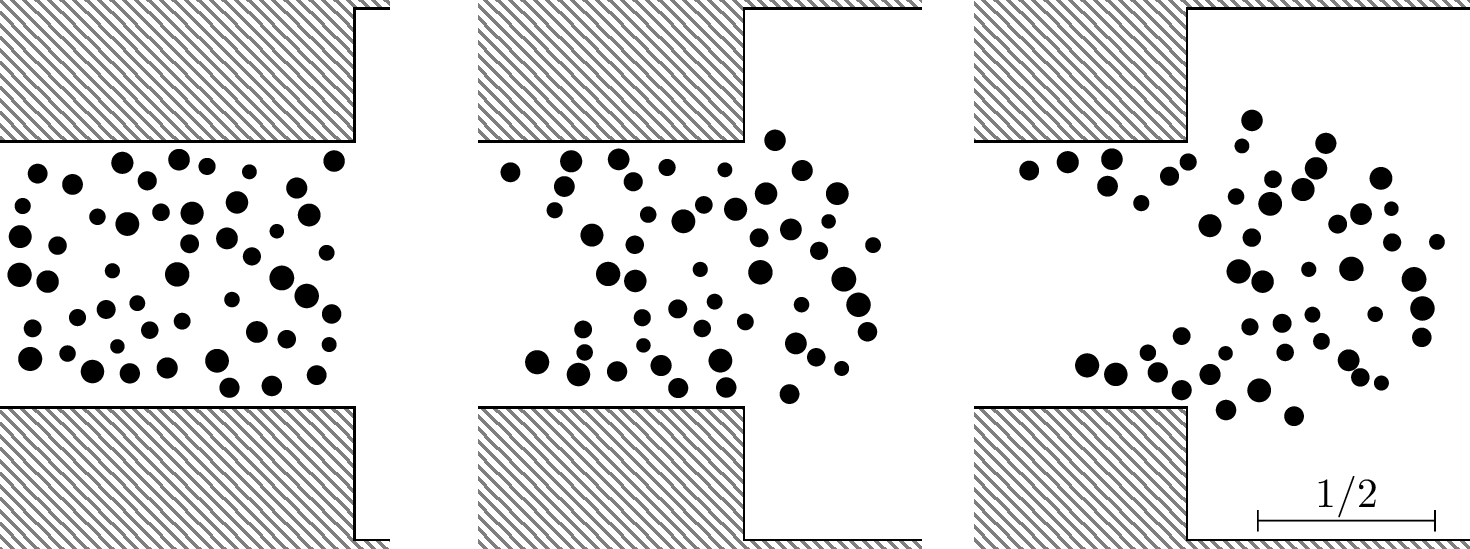
As a second, more realistic test, we consider a time-domain problem of the form 1 . The problem concerns the time-evolution of \(M=50\) droplets in a 2D rectangular pipe that suddenly widens, cf. 7. The flow is driven by a simple parabolic inflow profile, whereas no-slip conditions are imposed on the pipe boundaries. The initial positions and radii of the droplets are randomly chosen. We fix a timestep \(\Delta t=0.005\) and a number \(N_{\text{time}}=800\) of time-steps, reaching the time horizon \(t=t_{N_{\text{time}}}=4\).
Our ultimate target is approximating the \(M\) trajectories of each droplet’s center of mass. We compare four methods for approximating these:
CutFEM on a relatively fine mesh (\(\sim4\cdot 10^6\) DoFs). Since the droplets locations and shapes evolve in time, a time-dependent level-set function \(\phi=\phi(t,\mathbf{x})\) is used. Given the level-set function at time \(t\) and the fluid velocity \(\mathbf{u}(t,\mathbf{x})\) (computed by solving the Stokes equation with CutFEM 6.4), the level-set function at time \((t+\Delta t)\) is found by evolving the interface \(\Gamma(t)\) through a discretized version [25] of the advection equation \(\partial_t \phi + \mathbf{u}\cdot \nabla{\phi} = 0\), valid in the whole \(\Omega\) and with initial condition given from the level-set function at the previous time step. In order to avoid instabilities, the level-set function is reinitialized every \(5\) time steps as described in [29]. We treat the resulting trajectories from this scheme as “reference” in our tests. Each time-step takes about \(2\) minutes on our workstation, with \(\sim25\) seconds spent on CutFEM assembly, \(\sim75\) seconds spent on solving the discrete Stokes problem, and \(\sim20\) seconds spent to assemble and solve the level-set-advection equation. Level-set reinitialization takes \(\sim30\) additional seconds every \(5\) time steps.
Lowest-fidelity Stokes flow \(\mathbf{u}_0\). At each time-step, the droplets are advected as passive tracers, taking the mean of \(\mathbf{u}_0\) at \(n_{\text{adv}}=100\) markers uniformly distributed on each droplet’s boundary, cf. 13 . Since field \(\mathbf{u}_0\) is constant in time, this strategy is extremely cheap, taking only \(\sim0.4\) milliseconds per time-step. This time does not include the one-time overhead of computing \(\mathbf{u}_0\), which, since no droplets are present in 3 , can be done on a coarse mesh at extremely low cost (\(\sim4\) seconds on our workstation).
Our surrogate with the framework from 4.2. We use the same advection strategy as above, although the field approximation resulting from 3 replaces the time-independent Stokes flow \(\mathbf{u}_0\). At each time-step, our method performs \(5\) fixed-point iterations (automatically determined based on \(\mathrm{tol}\)) given the current droplet configuration, resulting in an average compute time of \(\sim1.5\) seconds per time-step. About \(80\%\) of this time is spent solving Stokes problems of the form 3 by FEM on a coarse mesh (using triangular solvers on LU-pre-factorized FEM matrices).
CutFEM without droplet deformations. We run the CutFEM code on the same mesh, but assuming that droplets do not deform and thus remain circular throughout the simulation. This assumption, consistently with our surrogate, slightly reduces the computational cost of advecting the droplets since the level set can be advected through rigid-body motion. Each time-step takes about \(100\) seconds, without the need for any reinitialization.
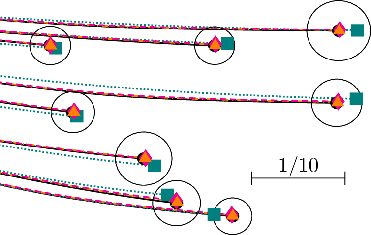
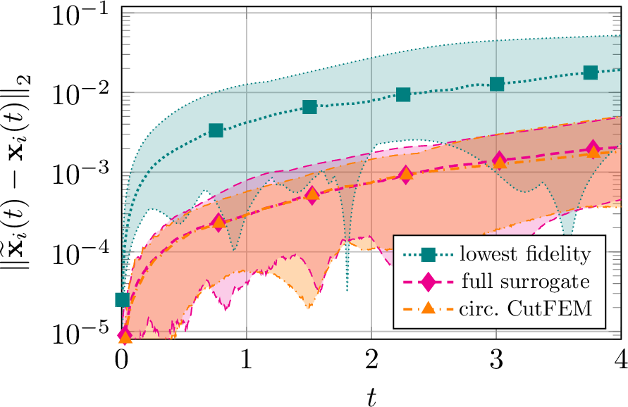
Figure 8: Left: Zoom of droplet trajectories near the bottom-right-most droplet. We show reference solution (black circles, full lines), lowest-fidelity surrogate (teal squares, dotted lines), full surrogate (magenta diamonds, dashed lines), and no-deformation CutFEM solution (orange triangles, dash-dotted lines). For readability, markers are shown only at the final time \(t=4\). Thin black lines denote boundaries of reference droplets at the final time. Right: error in lowest-fidelity, full surrogate, and no-deformation CutFEM trajectories over time. Each envelope shows the spread of the error, with lines marking the minimum, median, and maximum error over all droplets..
In 8 (left) we display some of the droplets’ trajectories obtained using the four methods. The surrogate trajectories are rather close to the reference ones, especially when compared to the lowest-fidelity results. This observation is confirmed quantitatively in 8 (right), where we show the trajectory approximation error. We can see that the full surrogate lowers the error by about an order of magnitude, compared to the lowest-fidelity approximation. Notably, the surrogate achieves a \(\times80\) speed-up with respect to the reference code while attaining a fair accuracy. The lowest-fidelity “passive-tracer” surrogate is also remarkable, since, despite a one-order-of-magnitude-larger error, it achieves a \(\times3\cdot10^5\) speed-up (excluding the single Stokes solve).
We look now at the non-deformable CutFEM results, whose computational cost is about \(60\) times larger than our full surrogate’s. As shown in 8 (right), the method’s accuracy is extremely close to our surrogate’s. This proves that the main source of error in our surrogate strategy is the circularity assumption, not the iterations or the subspace approximation of S_droplet. As such, we have good hopes for the accuracy achievable by our approach, once deformations are incorporated in the pipeline through future work.
As a final comparison, we also tried to run our CutFEM codes, both with and without droplet deformation, on a coarsened spatial mesh with about \(20\) times less degrees of freedom. The associated runtime per iteration was about \(9\) seconds in both cases, making these approaches comparable to our surrogate in terms of cost. However, the decreased computational cost comes with a decreased accuracy.
In particular, the coarsened results with deformation were wildly inaccurate due to droplets unphysically merging into “peanut” shapes due to the low mesh resolution (interfaces can merge if they intersect a single mesh element). Once merged, droplet pairs are pulled together by surface tension, thus increasing trajectory errors at further times. On the other hand, the errors in the non-deformable, coarsened test were only roughly twice as large as in the non-deformable, non-coarsened simulation. This seems to suggest that coarsening might be a beneficial strategy for time savings as long as droplets are handled as rigid bodies. However, we must mention that, in order to achieve this level of accuracy, we had to manually “turn off” surface tension to prevent the above-mentioned persistent errors due to merging, a strategy that is physically justified only if droplets are circular, cf. 3.
5.3 Scaling test↩︎
As a last numerical experiment, we investigate the scaling of our method, in terms of both accuracy and efficiency, as the number of droplets \(M\) increases. To this aim, we consider the static problem 2 over a rectangular domain with \(10^2\leq M\leq10^4\) droplets at (quasi-uniform) random locations. The droplets’ radii scale as \(r_i=\mathcal{O}(\sqrt M)\) to keep the “volume fraction” \(|\Omega_B|/|\Omega|\) constant at about \(20\%\). For simplicity, the flow is driven by parabolic inflow and outflow profiles at the left and right boundaries, respectively. See 2.
For each \(M\), the reference flow field is computed via CutFEM on a grid with \(\mathcal{O}(M)\) degrees of freedom. Note that the DoF scaling implies that the computational cost of the CutFEM solver scales approximately as \(\mathcal{O}(M)\), assuming an ideal cost of the linear-system solver. Such mesh refinement is needed in CutFEM in order to resolve the gaps between droplets but is optional in our method. Due to the high memory requirements for large \(M\) (e.g., \(\sim200\) GB for \(M=5000\)), the CutFEM simulations are run on a cluster (4 MPI nodes with an AMD EPYC 7742 CPU each).
The reference results are compared to the field produced by 3, which can be run on our workstation due to the much lower RAM requirements (e.g., \(\sim40\) GB for \(M=5000\), which can be drastically lowered at the cost of efficiency by reducing caching). For a fair comparison, after the surrogate is “trained” through 3, we evaluate the surrogate flow field on a fine grid with \(n_{\text{eval}}=\mathcal{O}(M)\) points, namely, the locations of the degrees of freedom in CutFEM. Incidentally, note that this large amount of evaluations is needed to compare surrogate and reference flows in the context of an error analysis, although it might be excessive in practical applications.
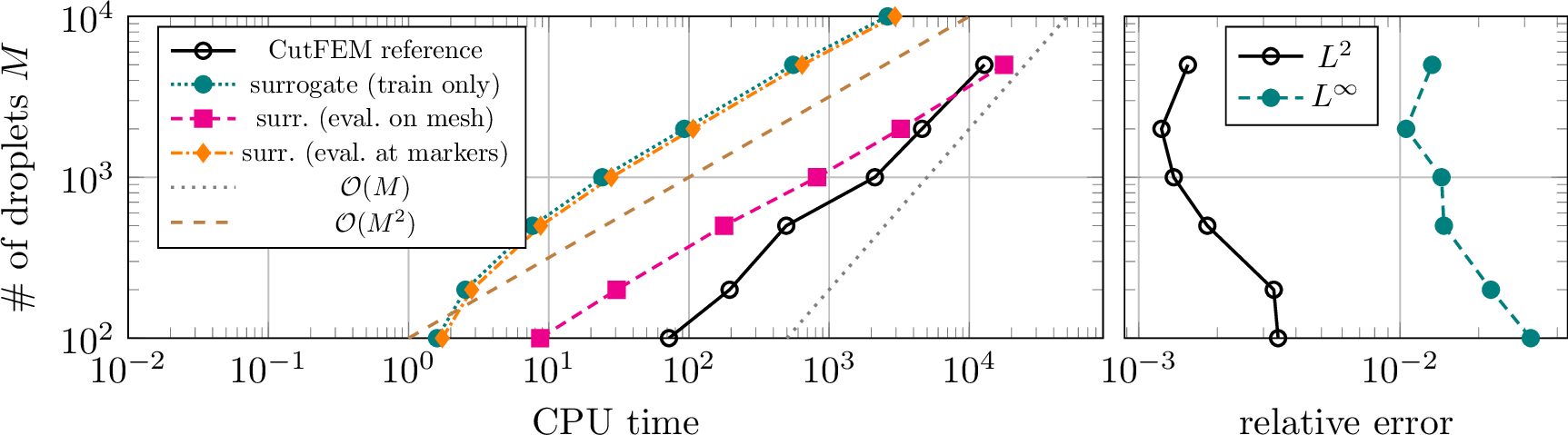
The results are summarized in 9. Therein, we can observe that, given the large number of evaluation points \(n_{\text{eval}}\), the surrogate evaluation takes almost \(100\) times longer than the surrogate training. In agreement with the analysis in 4, the surrogate evaluation at \(\mathcal{O}(M)\) points takes \(\mathcal{O}(M^2)\) time, with each point-evaluation taking \(\mathcal{O}(M)\) time.
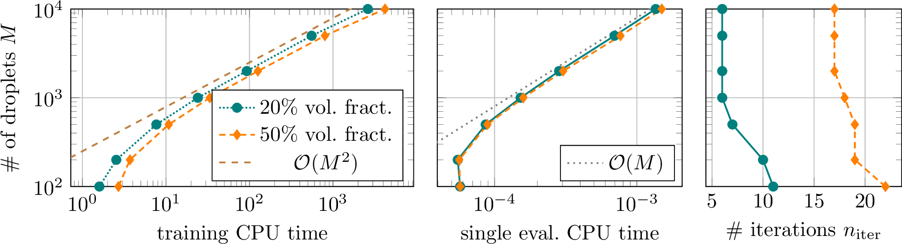
We observe the same quadratic scaling also in the surrogate training for large \(M\), which suggests that (i) the cost of solving Stokes problems (\(\text{S\_boundary}\) in 3) becomes negligible for large \(M\), as suggested in 4.1, and (ii) the number of fixed-point iterations \(n_{\text{iter}}\) remains roughly constant as \(M\) increases. In our experiments, we actually observed a decrease in \(n_{\text{iter}}\) as \(M\) increases, cf. 10 (right). This indicates that, at least in this setting with a fixed volume fraction, interaction effects between smaller droplets are easier to approximate through our method’s fixed-point iterations. As partial evidence supporting this, we note that the approximation error generally decreases as \(M\) increases even though \(D\) is kept constant, cf. 9 (right).
Including also the surrogate evaluation, our algorithm is more efficient than the reference CutFEM for \(M<5000\). At \(M=5000\) the surrogate’s quadratic scaling finally catches up with the almost linear cost of CutFEM. On the other hand, if one excludes the surrogate evaluation, our method is several orders of magnitude more efficient than the reference technique for all tested values of \(M\). This means that our surrogate-modeling strategy is competitive if a sufficiently small(er) number of evaluations is required. For instance, this happens when the target problem is a transient time evolution as in 4.2, which requires evaluating the surrogate field at \(100M\) total marker points (when \(n_{\text{adv}}=100\)), rather than at the \(\sim6700M\) CutFEM degrees of freedom. In both cases, \(n_{\text{eval}}\) scales linearly in \(M\), but with vastly different proportionality constants. The corresponding timings are also included in 9 (left) and 10 (center).
In order to show the effect of higher volume fraction on our method’s efficiency, we repeat our experiment with larger droplets, corresponding to \(|\Omega_B|/|\Omega|\simeq 50\%\). This results in stronger interactions between droplets, making more fixed-point iterations necessary to attain the same tolerance \(\mathrm{tol}\). This is shown in 10 (right), where we notice that \(n_{\mathrm{iter}}\) seems to stabilize at a (volume-fraction-dependent) value as \(M\) increases. This value represents a sort of “homogenized” (for \(M\to\infty\) with fixed volume fraction) fixed-point complexity for the corresponding volume fraction. Since a larger volume fraction generally yields smaller gaps between droplets as well as between droplets and domain boundaries, this result agrees with those presented in terms of contraction rate \(\rho_j\) in 6.
Despite this difference in number of iterations, the surrogate training costs increases only slightly with the volume fraction, cf. 10 (left). This is because the most expensive steps in 3, namely, the \(\mathcal{O}(M^2N)\) evaluations of the fundamental solutions \(\{\mathcal{S}(\widehat\boldsymbol{\phi}_k)\}_{k=1}^N\) in 11 , are cached at the first fixed-point iteration for efficiency, making the computational cost almost independent of the number of iterations. The surrogate evaluation costs are basically the same for both volume fractions, cf. 10 (center).
This test provides further evidence of how our method’s computational cost does not drastically blow up when the droplet interactions strengthen as a result of small gaps between droplets, e.g., those that might naturally arise in a time-domain simulation involving 1 . On the other hand, more standard discretization methods, e.g., based on CutFEM or boundary-integral equations, would face great difficulties in dealing with such small droplet gaps. While some evidence on this was provided in 5.2, we believe it would be of interest to carry out further, more detailed comparisons of our algorithm with other state-of-the-art methods.
6 Conclusions↩︎
We have presented a multi-fidelity surrogate modeling strategy for Stokes flows with large numbers of suspended droplets. The approach alternates between a background Stokes solver and precomputed single-droplet disturbance fields, using an iterative error-PDE correction to systematically capture droplet–flow, droplet–boundary, and droplet–droplet interactions. For geometrically similar droplets, an offline–online decomposition enables efficient reuse of single-droplet solutions. Numerical experiments demonstrate that the method maintains good accuracy across a wide range of configurations, including systems with up to \(10^4\) droplets. Even within a non-optimized implementation, the surrogate yields substantial speed-ups over fully resolved CutFEM simulations, demonstrating its potential to bring complex multiphase flow simulations within the reach of standard workstations, rather than requiring supercomputers.
The present framework naturally leads to several directions for future research. First, the fixed-point iteration underlying the method performed robustly in all tests, but a theoretical convergence analysis is missing. Second, extending the framework to deformable droplets appears to be within reach, as outlined in 3.5. Third, reducing the quadratic surrogate cost through hierarchical approximations of long-range droplet interactions inspired by fast-multipole methods, as outlined in 12, is a promising direction for further improving efficiency. Fourth, exploring whether aspects of the multi-fidelity framework can be generalized to Navier–Stokes flows is an interesting but very challenging direction.
Acknowledgements↩︎
This research was funded in part by the Wallenberg Academy Fellow grants KAW 2019.0190 and KAW 2024.0234.
Part of the computations were enabled by resources provided by the National Academic Infrastructure for Supercomputing in Sweden (NAISS), funded by the Swedish Research Council.
Appendix↩︎
6.1 Proof of 3↩︎
The proof proceeds by induction on \(j\), by showing that, for all \(j\), the claim from 3 holds, in addition to \[\label{eq:correctfullextra} \begin{cases} -\nabla\cdot{\boldsymbol{\sigma}}(\mathbf{u}_{j+1/2},p_{j+1/2};\mu)=\mathbf{f}+2(\mu-\mu_F)\nabla\cdot{\boldsymbol{\varepsilon}}(\mathbf{v}_{j+1/2}-\boldsymbol{\phi}_{j+1/2})&\text{in }\Omega_B\cup\Omega_F,\\ \nabla\cdot\mathbf{u}_{j+1/2}=0&\text{in }\Omega_B\cup\Omega_F,\\ \left\llbracket\mathbf{u}_{j+1/2}\right\rrbracket=\mathbf{0}&\text{on }\Gamma,\\ \left\llbracket{\boldsymbol{\sigma}}(\mathbf{u}_{j+1/2},p_{j+1/2};\mu)\mathbf{n}\right\rrbracket=\left(\gamma\kappa\mathrm{I}-2\left\llbracket\mu\right\rrbracket{\boldsymbol{\varepsilon}}(\mathbf{v}_{j+1/2}-\boldsymbol{\phi}_{j+1/2})|_{\Omega_B}\right)\mathbf{n}&\text{on }\Gamma, \end{cases}\tag{15}\] with \((\mathbf{u}_{j+1/2},p_{j+1/2})\) from 3.
6.1.0.1 Base case for \(j=0\).
We initialize \(\boldsymbol{\phi}_{-1/2}=\mathbf{v}_{-1/2}=\mathbf{u}_0\). The first claim, involving \((\mathbf{v}^{(0)},q^{(0)})\), follows by subtracting 3 and 4 from 2 equation by equation, cf. the inductive step.
In addition, we can show that 15 holds for \(j=0\) by linearity and by definition of \(\boldsymbol{\phi}_{1/2}\). For instance, fix one of the interfaces \(\Gamma_i\), \(i=1,\ldots,M\). On \(\Gamma_i\), by definition of \(\mathbf{v}_{0,i'}\) for \(i'\neq i\), we have \[\begin{align} \left\llbracket{\boldsymbol{\sigma}}(\mathbf{v}_{0,i'},q_{0,i'};\mu)\mathbf{n}\right\rrbracket=&\left\llbracket{\boldsymbol{\sigma}}(\mathbf{v}_{0,i'},0;\mu-\mu_F)\mathbf{n}\right\rrbracket+\left\llbracket{\boldsymbol{\sigma}}(\mathbf{v}_{0,i'},q_{0,i'};\mu_F)\mathbf{n}\right\rrbracket\\ =&2(\mu_F-\mu|_{\Omega_B^i}){\boldsymbol{\varepsilon}}(\mathbf{v}_{0,i'})|_{\Omega_B^i}\mathbf{n}+\mathbf{0}=2\left\llbracket\mu\right\rrbracket{\boldsymbol{\varepsilon}}(\mathbf{v}_{0,i'})|_{\Omega_B^i}\mathbf{n}, \end{align}\] whereas, by definition of \(\mathbf{v}_{0,i}\), cf. 7 , \[\left\llbracket{\boldsymbol{\sigma}}(\mathbf{v}_{0,i},q_{0,i};\mu)\mathbf{n}\right\rrbracket=-2\left\llbracket\mu\right\rrbracket{\boldsymbol{\varepsilon}}(\boldsymbol{\phi}_{-1/2})|_{\Omega_B^i}\mathbf{n}.\] From here we can use the previous claim and the definitions of \(\mathbf{u}\) and \(\boldsymbol{\phi}_{1/2}\) to show that \[\begin{align} \left\llbracket{\boldsymbol{\sigma}}(\mathbf{u}_{1/2},p_{1/2};\mu)\mathbf{n}\right\rrbracket=&\left\llbracket{\boldsymbol{\sigma}}(\mathbf{u}_0,p_0;\mu)\mathbf{n}\right\rrbracket+\sum_{i'=1}^M\left\llbracket{\boldsymbol{\sigma}}(\mathbf{v}_{0,i'},q_{0,i'};\mu)\mathbf{n}\right\rrbracket\\ =&\left\llbracket{\boldsymbol{\sigma}}(\mathbf{u},p;\mu)\mathbf{n}\right\rrbracket-\left\llbracket{\boldsymbol{\sigma}}(\mathbf{v}^{(0)},q^{(0)};\mu)\mathbf{n}\right\rrbracket+\left\llbracket{\boldsymbol{\sigma}}(\mathbf{v}_{0,i},q_{0,i};\mu)\mathbf{n}\right\rrbracket+\sum_{i'\neq i}\left\llbracket{\boldsymbol{\sigma}}(\mathbf{v}_{0,i'},q_{0,i'};\mu)\mathbf{n}\right\rrbracket\\ =&\gamma\kappa\mathbf{n}+2\left\llbracket\mu\right\rrbracket{\boldsymbol{\varepsilon}}(\boldsymbol{\phi}_{-1/2})|_{\Omega_B^i}\mathbf{n}-2\left\llbracket\mu\right\rrbracket{\boldsymbol{\varepsilon}}(\boldsymbol{\phi}_{-1/2})|_{\Omega_B^i}\mathbf{n}+2\left\llbracket\mu\right\rrbracket\sum_{i'\neq i}{\boldsymbol{\varepsilon}}(\mathbf{v}_{0,i'})|_{\Omega_B^i}\mathbf{n}\\ =&\gamma\kappa\mathbf{n}+2\left\llbracket\mu\right\rrbracket{\boldsymbol{\varepsilon}}({\textstyle\sum_{i'\neq i}\mathbf{v}_{0,i'}})|_{\Omega_B^i}\mathbf{n}=\gamma\kappa\mathbf{n}+2\left\llbracket\mu\right\rrbracket{\boldsymbol{\varepsilon}}(\boldsymbol{\phi}_{1/2}-\mathbf{v}_{1/2})|_{\Omega_B^i}\mathbf{n}, \end{align}\] with the final step following by inspection of \(\boldsymbol{\phi}_{1/2}|_{\Omega_B^i}\), cf. 4. A similar derivation can be carried out also within the droplet \(\Omega_B^i\).
6.1.0.2 Inductive step for \(j>0\).
The claim in 3, involving \((\mathbf{v}^{(j)},q^{(j)})\), can be proved by leveraging the linearity of the PDE and the inductive hypothesis on both the main claim of 3 and 15 . For instance, by construction of \(\mathbf{v}_{j-1/2}\), on \(\Gamma\) we have \[\begin{align} \left\llbracket{\boldsymbol{\sigma}}(\mathbf{v}_{j-1/2},q_{j-1/2};\mu)\mathbf{n}\right\rrbracket=&\left\llbracket{\boldsymbol{\sigma}}(\mathbf{v}_{j-1/2},0;\mu-\mu_F)\mathbf{n}\right\rrbracket+\left\llbracket{\boldsymbol{\sigma}}(\mathbf{v}_{j-1/2},q_{j-1/2};\mu_F)\mathbf{n}\right\rrbracket\\ =&2(\mu_F-\mu|_{\Omega_B}){\boldsymbol{\varepsilon}}(\mathbf{v}_{j-1/2})|_{\Omega_B}\mathbf{n}+\mathbf{0}=2\left\llbracket\mu\right\rrbracket{\boldsymbol{\varepsilon}}(\mathbf{v}_{j-1/2})|_{\Omega_B}\mathbf{n}, \end{align}\] so that, by inductive assumption, \[\begin{align} \left\llbracket{\boldsymbol{\sigma}}(\mathbf{u}_j,p_j;\mu)\mathbf{n}\right\rrbracket=&\left\llbracket{\boldsymbol{\sigma}}(\mathbf{u}_{j-1/2},p_{j-1/2};\mu)\mathbf{n}\right\rrbracket+\left\llbracket{\boldsymbol{\sigma}}(\mathbf{v}_{j-1/2},q_{j-1/2};\mu)\mathbf{n}\right\rrbracket\\ =&\gamma\kappa\mathbf{n}+2\left\llbracket\mu\right\rrbracket{\boldsymbol{\varepsilon}}(\boldsymbol{\phi}_{j-1/2}-\mathbf{v}_{j-1/2})|_{\Omega_B}\mathbf{n}+2\left\llbracket\mu\right\rrbracket{\boldsymbol{\varepsilon}}(\mathbf{v}_{j-1/2})|_{\Omega_B}\mathbf{n}\\ =&\gamma\kappa\mathbf{n}+2\left\llbracket\mu\right\rrbracket{\boldsymbol{\varepsilon}}(\boldsymbol{\phi}_{j-1/2})|_{\Omega_B}\mathbf{n}. \end{align}\] Recalling the definition of \((\mathbf{u},p)\), we deduce that, on \(\Gamma\), \[\left\llbracket{\boldsymbol{\sigma}}(\mathbf{v}^{(j)},q^{(j)};\mu)\mathbf{n}\right\rrbracket=\left\llbracket{\boldsymbol{\sigma}}(\mathbf{u},p;\mu)\mathbf{n}\right\rrbracket-\left\llbracket{\boldsymbol{\sigma}}(\mathbf{u}_j,p_j;\mu)\mathbf{n}\right\rrbracket=-2\left\llbracket\mu\right\rrbracket{\boldsymbol{\varepsilon}}(\boldsymbol{\phi}_{j-1/2})|_{\Omega_B}\mathbf{n}.\] A similar derivation can be carried out also within the droplet \(\Omega_B^i\).
From here, by following the same steps as in the base case we can show that 15 holds true. This is sufficient for the next induction step.
6.2 Change of coordinates in second-fidelity problem↩︎
For an arbitrary \(\mathbf{x}_i\in\mathbb{R}^d\) and \(r_i>0\), define the affine function \(\eta_i(\mathbf{x})=r_i\mathbf{x}+\mathbf{x}_i\), which maps the unit disk \(\Omega_B^\sharp\) to \(\Omega_B^i\). We consider problem 5 with \(\Omega_B^i=B(\mathbf{x}_i;r_i)\), \(\boldsymbol{\phi}\in[H^1(\Omega_B^i)]^d\) smooth enough, and \(\mu=\mu_F+(\mu(\mathbf{x}_i)-\mu_F)\chi_{\Omega_B^i}\).
Let \(\widehat\mathbf{v}:=\mathbf{v}\circ\eta_i\), \(\widehat q:=r_i q\circ\eta_i\), \(\widehat\mu:=\mu\circ\eta_i\), and \(\widehat\boldsymbol{\phi}:=\boldsymbol{\phi}\circ\eta_i\). Moreover, by the chain rule, let \(\widehat\nabla:=r_i\nabla\) and \(\widehat{\boldsymbol{\sigma}}(\widehat\mathbf{v}(\cdot),\widehat q(\cdot);\widehat\mu)=r_i{\boldsymbol{\sigma}}(\mathbf{v}(\cdot),q(\cdot);\mu)\circ\eta_i\), which involve differential operators in the reference coordinates \(\eta_i^{-1}(\mathbf{x})\). It follows that \[\begin{cases} -r_i^{-1}\widehat\nabla\cdot\left(r_i^{-1}\widehat{\boldsymbol{\sigma}}(\widehat\mathbf{v},\widehat q;\widehat\mu)\right)=(\widehat\mu-\mu_F)r_i^{-1}\widehat\nabla\cdot\left(r_i^{-1}\widehat{\boldsymbol{\varepsilon}}(\widehat\boldsymbol{\phi})\right)&\mathrm{in }\mathbb{R}^d\setminus\partial \Omega_B^\sharp,\\ r_i^{-1}\widehat\nabla\cdot\widehat\mathbf{v}=0&\mathrm{in }\mathbb{R}^d\setminus\partial \Omega_B^\sharp,\\ \left\llbracket\widehat\mathbf{v}\right\rrbracket=\mathbf{0}&\mathrm{on }\partial \Omega_B^\sharp,\\ \left\llbracket r_i^{-1}\widehat{\boldsymbol{\sigma}}(\widehat\mathbf{v},\widehat q;\widehat\mu)\mathbf{n}\right\rrbracket=r_i^{-1}\left(\gamma\kappa\mathrm{I}-\left\llbracket\widehat\mu\right\rrbracket\widehat{\boldsymbol{\varepsilon}}(\widehat\boldsymbol{\phi})\right)\mathbf{n}&\mathrm{on }\partial \Omega_B^\sharp,\\ \lim_{\left\|\mathbf{x}\right\|\to\infty}\widehat\mathbf{v}(\mathbf{x})=\mathbf{0}. \end{cases}\] After canceling out the powers of \(r_i\), we see that this problem is equivalent to 5 with \(\Omega_B^i=\Omega_B^\sharp\), \(\widehat\boldsymbol{\phi}\) as forcing flow field, and \(\mu=\widehat\mu\).
6.3 Polynomial basis in dimension two↩︎
In 3, we only apply \(\text{S\_droplet}\), i.e., \(\mathcal{S}\) from 10 , to fields \(\boldsymbol{\phi}\) that satisfy the homogeneous Stokes equation over \(\Omega_B^i\), i.e., that belong to the space of smooth, compatible flow fields \[\mathcal{V}=\left\{\mathbf{v}\in[C^3(\mathbb{R}^d)]^2,\nabla\cdot\mathbf{v}\equiv0,\nabla\times\nabla\cdot{\boldsymbol{\varepsilon}}(\mathbf{v})\equiv0\right\}.\] The last condition above encodes a compatibility condition, ensuring that, for each element \(\mathbf{v}\in\mathcal{V}\), one can find a pressure field \(q\in C^2(\mathbb{R}^d)\) satisfying the homogeneous Stokes equation \(\nabla\cdot{\boldsymbol{\sigma}}(\mathbf{v},q;\mu_F)=\mathbf{0}\) [30], [31]. To compute a (polynomial) basis of \(\mathcal{V}\) in \(d=2\) dimensions, we use stream functions.
Recall that, in \(\mathbb{R}^2\), \(\mathcal{V}=\nabla^\perp\mathcal{W}\), with \(\nabla^\perp=[-\partial_{x_2},\partial_{x_1}]^\top\) and with \(\mathcal{W}\) being the space of biharmonic scalar fields [31] \[\mathcal{W}=\left\{\phi\in C^4(\mathbb{R}^2),\nabla\cdot\nabla(\nabla\cdot\nabla\phi)\equiv0\right\}.\] A hierarchical polynomial basis of \(\mathcal{W}\) can be easily constructed as [30] \[\mathcal{W}=\text{span}\bigcup_{n=0}^\infty\left\{\rho\psi\in\mathbb{P}^n(\mathbb{R}^2),\text{deg}(\rho\psi)=n,\rho(\mathbf{x})\in\{1,x_1^2+x_2^2\},\nabla\cdot\nabla\psi\equiv0\right\}.\] In turn, harmonic polynomials \(\psi\) on \(\mathbb{R}^2\) are easily expressible through holomorphy arguments as real or imaginary parts of polynomials in \((x_1+\mathrm{i}x_2)\). Accordingly, a hierarchical (in total degree) basis of \(\mathcal{W}\) is found: \[\begin{gather} \mathcal{W}=\text{span}\bigg(\left\{1\right\}\cup\left\{x_1,x_2\right\}\cup\left\{x_1^2-x_2^2,2x_1x_2,x_1^2+x_2^2\right\}\cup\\\cup\bigcup_{n=3}^\infty\left\{\text{Re}\left((x_1+\mathrm{i}x_2)^n\right),\text{Im}\left((x_1+\mathrm{i}x_2)^n\right),(x_1^2+x_2^2)\text{Re}\left((x_1+\mathrm{i}x_2)^{n-2}\right),(x_1^2+x_2^2)\text{Im}\left((x_1+\mathrm{i}x_2)^{n-2}\right)\right\}\bigg). \end{gather}\] From here, a polynomial basis for the space \(\mathcal{V}=\nabla^\perp\mathcal{W}\) of compatible flow fields can be derived by linearity of the differential operator involved.
Note that, since differentiations is involved to extract flow fields from stream functions, and since \(\boldsymbol{\phi}\) enters 5 only through its strain field \({\boldsymbol{\varepsilon}}(\boldsymbol{\phi})\), constant and linear basis functions of \(\mathcal{W}\) are irrelevant and can be discarded. Additionally, the quadratic stream function \(\phi(\mathbf{x})=x_1^2+x_2^2\) yields a strain-free rotation field and can thus be ignored: \[{\boldsymbol{\varepsilon}}\left(\nabla^\perp(x_1^2+x_2^2)\right)={\boldsymbol{\varepsilon}}\left([-2x_2,2x_1]^\top\right)=\begin{pmatrix}0&0\\0&0\end{pmatrix}.\] Truncating the basis of \(\mathcal{W}\) at degree \((D+1)\), with \(D\geq1\), yields a degree-\(D\) basis for \(\mathcal{V}\) with dimension \(4D-2\).
When precomputing the fundamental solutions corresponding to the above basis functions, the computational effort may be reduced by exploiting the symmetry of stream functions. This can be used to cut the precomputation time in half.
6.4 CutFEM setup↩︎
Denote \(\mathcal{K}_h\) a regular partition of \(\Omega\) which does not need to conform to the interfaces \(\Gamma\) inside \(\Omega\) but conforms to the polygonal boundary \(\partial \Omega\). Associated with the subdomain \(\Omega_B\) and \(\Omega_F\), and with the interfaces \(\Gamma\), we define the active meshes: \[\mathcal{K}_{h,\bullet} = \left\{K \in \mathcal{K}_h,\;K \cap \Omega_i \neq \emptyset\right\}, \;\bullet=B,F, \quad\text{and}\quad \mathcal{K}_{h,\Gamma} = \left\{K \in \mathcal{K}_h,\;|\Gamma \cap \bar{K}| > 0\right\}.\] From the active meshes, we define the active domain \[\Omega_{h,\bullet} = \bigcup_{K \in \mathcal{K}_{h,\bullet}} K, \quad\bullet=B,F\] and the approximate interface \(\Gamma_h\) as a piecewise-polynomial approximation of \(\Gamma\).
Let \(\mathcal{V}_h^\mathbf{u}\) and \(\mathcal{V}_h^p\) be the Taylor-Hood elements P2-P1 on \(\mathcal{K}_h\). The active finite-element space is then the restriction to the active domain: \[\mathcal{V}_{h,\bullet}^\mathbf{u}= \mathcal{V}_h^\mathbf{u}|_{\Omega_{h,\bullet}}\quad\text{and}\quad\mathcal{V}_{h,\bullet}^p = \mathcal{V}_h^p|_{\Omega_{h,\bullet}} , \quad \bullet=B,F,\] and we let \[\begin{align} V_h^\mathbf{u}&= \mathcal{V}_{h,B}^\mathbf{u}\times \mathcal{V}_{h,F}^\mathbf{u}= \left\{ \mathbf{v}_h = (\mathbf{v}_{h,B}, \mathbf{v}_{h,F}) , \;\mathbf{v}_{h,\bullet}\in \mathcal{V}_{h,\bullet}^\mathbf{u}, \;\bullet=B,F \right\},\\ V_h^p& = \mathcal{V}_{h,B}^p \times \mathcal{V}_{h,F}^p = \left\{ q_h = (q_{h,B}, q_{h,F}) , \;q_{h,\bullet}\in \mathcal{V}_{h,\bullet}^p, \;\bullet=B,F \right\}. \end{align}\]
The weak formulation of 2 is: find \((\mathbf{u}_h, p_h) \in V_h^{\mathbf{u}} \times V_h^{p}\) such that \[a(\mathbf{u}_h, \mathbf{v}_h) + \tau_\mathbf{u}s_\mathbf{u}( \mathbf{u}_h, \mathbf{v}_h) + b(\mathbf{u}_h, q_h) - b(\mathbf{v}_h, p_h) + \tau_p s_p(p_h,q_h) = l(\mathbf{v}_h, q_h)\quad\forall (\mathbf{v}_h, q_h) \in V_h^{\mathbf{u}} \times V_h^{p},\] Above, \[\begin{align} a(\mathbf{u}_h,\mathbf{v}_h) & = \sum_{\bullet\in\{B,F\}}\left(2\mu{\boldsymbol{\varepsilon}}(\mathbf{u}_h),{\boldsymbol{\varepsilon}}(\mathbf{v}_h)\right)_{\Omega_{h,\bullet}} - \left(\lbrace 2\mu {\boldsymbol{\varepsilon}}(\mathbf{u}_h) \mathbf{n}\rbrace, \left\llbracket\mathbf{v}_h\right\rrbracket\right)_{\Gamma_h} - \left(\left\llbracket\mathbf{u}_h\right\rrbracket,\lbrace 2\mu {\boldsymbol{\varepsilon}}(\mathbf{v}_h) \mathbf{n}\rbrace\right)_{\Gamma_h}\\ & + \lambda_{\Gamma}\left(\left\llbracket\mathbf{u}_h\right\rrbracket,\left\llbracket\mathbf{v}_h\right\rrbracket\right)_{\Gamma_h} - \left(2\mu {\boldsymbol{\varepsilon}}(\mathbf{u}_h) \mathbf{n},\mathbf{v}_h\right)_{\Gamma_D} - \left(\mathbf{u}_h,2\mu {\boldsymbol{\varepsilon}}(\mathbf{v}_h) \mathbf{n}\right)_{\Gamma_D} + \lambda_D\left(\mathbf{u}_h,\mathbf{v}_h\right)_{\Gamma_D},\\ b(\mathbf{u}_h,q_h) & = \sum_{\bullet\in\{B,F\}}\left(\nabla \cdot \mathbf{u}_h,q_h\right)_{\Omega_{h,\bullet}} - \left(\left\llbracket\mathbf{u}_h \cdot \mathbf{n}\right\rrbracket, \lbrace q_h\rbrace\right)_{\Gamma_h} - \left(\mathbf{u}_h \cdot \mathbf{n},q_h\right)_{\Gamma_D},\\ l(\mathbf{v}_h,q_h) & = \sum_{\bullet\in\{B,F\}}\left(\mathbf{f},\mathbf{v}_h\right)_{\Omega_h,\bullet} + \left(\gamma \kappa \mathbf{n},\lbrace\mathbf{v}_h\rbrace\right)_{\Gamma_h} - \left(\mathbf{g}_N,\mathbf{v}_h\right)_{\Gamma_N}\\ &- \left(\mathbf{g}_D, 2\mu {\boldsymbol{\varepsilon}}(\mathbf{v}_h) \mathbf{n}\right)_{\Gamma_D} + \lambda_D\left(\mathbf{g}_D, \mathbf{v}_h\right)_{\Gamma_D} - \left(\mathbf{g}_D\cdot \mathbf{n},q_h\right)_{\Gamma_D}, \end{align}\] with \((\cdot,\cdot)_A\) the \(L^2(A)\)-inner product and \(\lbrace f\rbrace=\frac{1}{2}(f|_{\Omega_B}+f|_{\Omega_F})\) the average across \(\Gamma_h\).
Given the set of edges \(\mathcal{E}_{h,\bullet}\) of each active mesh \(\mathcal{K}_{h,\bullet}\), we define the stabilization terms \(s_\mathbf{u}\) and \(s_p\) as \[\begin{align} s_\mathbf{u}(\mathbf{u}_h,\mathbf{v}_h) & = \sum_{\bullet\in\{B,F\}} \sum_{e \in \mathcal{E}_{h,\bullet}}\left(h\left(\left\llbracket\partial_{\mathbf{n}_e}\mathbf{u}_{h,\bullet}\right\rrbracket_e,\left\llbracket\partial_{\mathbf{n}_e}\mathbf{v}_{h,\bullet}\right\rrbracket_e\right)_e + h^3\left(\left\llbracket\partial_{\mathbf{n}_e}^2\mathbf{u}_{h,\bullet}\right\rrbracket_e,\left\llbracket\partial_{\mathbf{n}_e}^2\mathbf{v}_{h,\bullet}\right\rrbracket_e\right)_e\right),\\ s_p(p_h,q_h) & = \sum_{\bullet\in\{B,F\}} \sum_{e \in \mathcal{E}_{h,\bullet}}h^3\left(\left\llbracket\partial_{\mathbf{n}_e}p_{h,\bullet}\right\rrbracket_e,\left\llbracket\partial_{\mathbf{n}_e}q_{h,\bullet}\right\rrbracket_e\right)_e, \end{align}\] with \(\mathbf{n}_e\) the unit normal to edge \(e\) and \(\left\llbracket\cdot\right\rrbracket_e\) the jump across edge \(e\), both with arbitrary but fixed sign.
References↩︎
Stockholm University, Stockholm, Sweden (davide.pradovera@math.su.se).↩︎
KTH Royal Institute of Technology, Stockholm, Sweden (frachon@kth.se, sara.zahedi@math.kth.se).↩︎
We use the subscript “\(B\)” (standing for “bubbles”) rather than “\(D\)” (for “droplets”) to avoid misunderstandings with Dirichlet boundary notation.↩︎
If \(\Gamma_N=\emptyset\), well-posedness requires supplementing the problem with a zero-mean condition on the pressure, \(\int_\Omega p=0\). This condition can be imposed in post-processing once a solution has been obtained and does not affect the present discussion.↩︎
This not-so-trivial property holds true due to two combined properties: (i) the linearity of the \((M+1)\) PDEs solved at each iteration and (ii) the exactness of all full-step approximations \((\mathbf{u}_j,p_j)\) in terms of boundary conditions.↩︎
An adaptive time-stepping scheme based on the surrogate solution may of course be applied, e.g., where finer steps are taken if droplets are about to collide.↩︎