Complexity of Normalized Persistence Problems
for Topological Data Analysis and Local Hamiltonians
July 03, 2026
Abstract
Topological data analysis (TDA) is a machine learning technique that uses topology to extract patterns from data and has shown the potential to exhibit quantum advantage. A key concept in TDA is persistent homology, which measures the robustness of topological information at different lengthscales. In this paper, we introduce and study the problem of normalized persistence, a practically motivated and easily interpretable version of persistent homology that counts the fraction of holes that persist at different lengthscales. We prove that a variant of normalized persistence is \(\mathsf{DQC}_1\)-hard and contained in \(\mathsf{BQP}\), giving evidence of an exponential quantum speedup for TDA under the standard assumption that \(\mathsf{DQC}_1 \not\subseteq \mathsf{BPP}\). These are the first DQC\(_1\)-hardness results that are directly applicable to TDA instances. We also find a close connection between normalized persistence and the complexity of estimating spectral quantities in the low-energy subspace of local Hamiltonians. We study a family of such problems, including a low-energy normalized subtrace and spectral density. We show that these are \(\mathsf{DQC}_1\)-hard for \(O(1)\)-local Hamiltonians, strengthening previous results that required log-local interactions. We also introduce a variant of DQC\(_1\) with perfect completeness (SDQC\(_1\)) to characterize the hardness of problems normalized by an exact kernel. This includes normalized persistence for \(O(1)\)-local Hamiltonians, which we show is SDQC\(_1\)-hard.
YITP-26-81
1 Overview↩︎
1.1 Motivation↩︎
Topological data analysis (TDA) is a technique that uses tools from algebraic topology to study properties of data. It is a mature field in machine learning [1] with several applications [2], [3], and has gained attention as a task that may exhibit quantum advantage. TDA works by taking data and forming a ‘simplicial complex’ \(X\), a topological space consisting of higher-dimensional triangles (simplices). One can then use algebraic topology to calculate the number of \(d\)-dimensional holes in the complex, revealing information about the manifold that the data was drawn from. The number of \(d\)-dimensional holes in \(X\) is called the \(d\)’th Betti number and denoted by \(\beta_d^X\). The original quantum TDA algorithm [4] outputs the normalized Betti number \(\beta_d^X/|X_d|\), where \(|X_d|\) is the number of \(d\)-simplices in the complex. In practical TDA applications one is also interested in how many holes persist from one complex to another, when both are formed from the same dataset. This motivates the persistent Betti number \(\beta^{1,2}_d\), the number of \(d\)-dimensional holes present in a complex \(X_1\) that are also present in a larger complex \(X_2\). Indeed a quantum algorithm for the normalized persistent Betti number \(\beta^{1,2}_d/|X_{1,d}|\) was developed in [5]. Determining the computational complexity of these quantities has remained an open problem since these algorithms were proposed, with DQC\(_1\)-hardness of the normalized Betti number being a central unresolved question [6]. Recall that DQC\(_1\) is the class of problems that can be solved efficiently on a quantum computer with one clean qubit and other qubits starting in the maximally mixed state. For example, normalized trace estimation and Jones polynomial estimation are known to be DQC\(_1\)-complete [7], which can be seen as evidence of classical hardness for DQC\(_1\)-hard problems because we do not know efficient classical algorithms for them. Moreover, it is known that it is classically hard to sample from DQC\(_1\)-circuits under plausible complexity theoretic assumptions [8]. We give a more in-depth overview of the topology preliminaries in Section [sec:prelim95topo].
In this paper we consider an alternative normalized quantity: the normalized persistence \[\label{eqn:32Normalized32persistence} \frac{\beta_d^{1,2}}{\beta_d^1},\tag{1}\] the fraction of \(d\)-dimensional holes present in a complex \(X_1\) that persist into a complex \(X_2\). The difference in normalization is practically motivated, since the quantity gives an easily interpretable measure of how robust the topological features are in the initial complex. Indeed, one of the key reasons for studying persistence in TDA is that holes which persist are less likely to be the result of noise in the data and more likely to be true features of the underlying manifold. In addition, since the normalized persistence is not governed by the simplex count \(|X_d|\) it allows for reasonable comparison between the complexes on different datasets. The main goal of this paper is to study the computational complexity of normalized persistence and a family of related quantities.
A key insight of this work is that normalized persistence is naturally a low-energy subspace problem. It is known that Betti numbers are equivalent to the kernel dimensions of Hermitian operators, namely combinatorial Laplacians. Persistent Betti numbers can then be expressed through the overlap of kernels under an inclusion. This gives an immediate generalization of the problems we consider to low (or zero) energy subspace problems for local Hamiltonians, whose complexity we also study. These analogous Hamiltonian problems consist of estimating various spectral or overlap quantities in the low-energy subspace, with suitable normalization. In many physically relevant scenarios, the state of interest lies in the low-energy subspace of a local Hamiltonian, rather than the full Hilbert space. For example, low-energy states of quantum many body systems are typically described by a quantum field theory in the thermodynamic limit [9]. The utility of the low-energy subspace can also be seen in quantum algorithms. Recent work on Hamiltonian simulation shows that restricting to this subspace leads to algorithms whose simulation error depends on an effective low-energy norm, rather than the full operator norm [10], [11]. The relevance of the low-energy subspace can also be seen with practical implementations of quantum computers, since a physical qubit is typically obtained by isolating two energy levels from the rest of the spectrum. This motivates a second key goal of this paper, to establish \(\mathsf{DQC}_1\)-hardness for \(O(1)\)-local Hamiltonian problems restricted to low-energy subspaces. This is a setting directly inspired by the normalized persistence problem, and a strengthening of the previously known log-local results.
Previous work [6] has formalized the problem of approximating \(\beta_d/|X_d|\), as ‘Approximate Betti Number Estimation’. Whilst the complexity of this is still open, Gyurik et al. establish a connection with Low-Lying Spectral Density (LLSD). This problem estimates the number of eigenvalues of a Hamiltonian below a given threshold, normalized by the full Hilbert space dimension (see Problem 11), and is only known to be DQC\(_1\)-hard for log-local Hamiltonians. In [12] Cade and Crichigno established \(\mathsf{DQC}_1\)-hardness of normalized quasi-Betti number estimation. This is estimation of the dimension of the low-energy subspace of a combinatorial Laplacian divided by the dimension of the chain space. However, their result only holds for log-local co-boundary operators and does not hold for clique complexes, which are the complexes arising in TDA. When studying normalized persistence, the more relevant underlying problem replaces the \(2^n\) normalization of LLSD with the dimension of the low-energy subspace; we call this variant the low-energy spectral density (\(\textsf{LESD}\)). We prove that it is DQC\(_1\)-hard and contained in BQP. In contrast to these previous results, this DQC\(_1\)-hardness result holds for Laplacians of clique complexes. On the Hamiltonian side we are able to show that LESD is DQC\(_1\)-hard for \(O(1)\)-local Hamiltonians, strengthening the previous log-local results for LLSD. We also establish DQC\(_1\)-hardness for a variant of normalized persistence, again applying to clique complexes. These results form the first DQC\(_1\)-hardness results for the practical structures arising in TDA, and therefore serve as a step towards resolving whether ‘Approximate Betti Number Estimation’ is DQC\(_1\)-hard.
We show that all the problems considered in this paper are contained in BQP, under state preparation and overlap assumptions. For the problems that are DQC\(_1\)-hard, we are also able to show that this hardness holds with the assumptions for containment in BQP. Thus under the standard assumption that \(\textsf{DQC_1}\not\subseteq \textsf{BPP}\), this work establishes several exponential quantum advantages for problems in TDA and for local Hamiltonians in the worst-case. In order to study problems involving the exact kernel, we introduce a variant of DQC\(_1\) with perfect completeness which we call SDQC\(_1\). Similarly, if this class is classically hard to simulate, our results will imply an exponential quantum advantage for these problems also.
We next review the related literature in more detail. Readers primarily interested in our contributions can safely skip to the summary of our main results in Section 1.3.
1.2 Existing Literature↩︎
1.2.1 Complexity results for TDA↩︎
In recent years a plethora of results on the complexity of various tasks within TDA have emerged. Schmidhuber and Lloyd showed that exact computation of Betti numbers is \(\#\mathsf{P}\)-hard and approximating them to multiplicative error is NP-hard [13]. Crichigno and Kohler [14] showed that the problem of deciding whether \(\beta_d>0\) (referred to as clique homology) is \(\textsf{QMA}_1\)-hard. Note this also implies that approximating \(\beta_d\) to multiplicative error is \(\textsf{QMA}_1\)-hard, strengthening the results of Schmidhuber and Lloyd. The authors also show containment in QMA, but for a gapped version of the problem with a promised lower bound on the smallest eigenvalue of the Laplacian in NO instances. King and Kohler [15] show that this gapped version of clique homology is \(\textsf{QMA}_1\)-hard and contained in \(\textsf{QMA}\), but for weighted clique complexes. Rudolph [16] showed that gapped clique homology on weighted clique complexes is \(\textsf{QMA} _1\)-complete (with a suitable gateset), improving on the results of King and Kohler. Moreover, the author shows that standard clique homology (unweighted and without promise) is PSPACE-complete, strengthening the results of Crichigno and Kohler further. It has also been shown that estimating the minimum eigenvalue of a weighted combinatorial Laplacian is QMA-hard [17]. Finally, Hayakawa et al. show that there exist restricted versions of clique homology that are MA-complete [18].
In related works, it was shown that deciding whether a given hole persists from one complex to another is \(\textsf{BQP}_1\)-hard and contained in BQP [19]. Although this result provides evidence of exponential quantum advantage for deciding persistence of a hole, it does not tell the complexity of learning the persistence of all the holes in the initial simplicial complex.
1.2.2 Quantum algorithms for TDA↩︎
A parallel line of work has developed quantum algorithms for tasks in TDA. The first quantum algorithm was given by Lloyd, Garnerone, and Zanardi [4] and gives a way to estimate the normalized Betti number \(\beta_d/|X_d|\). Subsequent works refined this approach by improving the resource requirements of the original algorithm, for example through shorter circuit-depth constructions [20]. The framework has also been extended from Betti numbers of a single complex to persistent Betti numbers [5], [21]. There has also been work on related topological tasks, such as harmonic persistence [19], high-dimensional Dirichlet problems via quantum walks [22], and torsion detection [23].
At the same time, the regimes in which these algorithms can yield substantial quantum speedups are subtle. A detailed resource analysis was given by Berry et al. [24], and dequantized algorithms have been developed for estimating Betti numbers [21], [24], [25]. These results narrow the parameter regimes in which a quantum advantage is expected.
Moreover, although there has been substantial effort on the analysis of the quantum complexity landscape in TDA, a full understanding of the complexity of normalized Betti number estimation remains open. This motivates the study of the computational complexity of normalized quantities in TDA themselves.
1.3 Main Results↩︎
Here we outline the key results of this paper. This is not exhaustive, as we also prove hardness and containment results for various other problems that are used in our chain of reductions. A summary of our intermediate results is outlined in Section 1.5 and can also be seen in Table 1. A more detailed view of how the hardness of these problems relate to each other, as well as connections to problems from previous works, is given in Figure 1.
| Problem | Hardness | Containment |
|---|---|---|
| Normalized Subtrace, Prob. [prob:NST] | \(\mathsf{DQC}_1\) [26] | \(\mathsf{DQC}_1\) [12] |
| Low-lying Spectral Density (LLSD), Prob. [prob:LLSD] | \(\mathsf{DQC}_1\) [6] | \(\mathsf{DQC}_1\) [6] |
| Low-energy Normalized Subtrace (LENS), Prob. [prob:LENS] | \(\mathsf{DQC}_1\) (Thm [thm:32low32energy32subtrace]) | \(\mathsf{BQP}\) (Lem [lemma:containment95LENS]) |
| Low-energy Spectral Density (LESD), Prob. [prob:LESD] | \(\mathsf{DQC}_1\) (Thm [thm:32LESD]) | \(\mathsf{BQP}\) (Lem [lemma:containment95LESD]) |
| Low-energy Kernel Density (LEKD), Def. [prob:LEKD] | \(\mathsf{SDQC}_1\) (Thm [thm:LEKD95hardness]) | \(\mathsf{BQP}\) (Lem [lemma:containment95LEKD]) |
| Normalized Quasi-Persistence (NQP), Prob. [prob:normalized95quasi95persistence] | \(\mathsf{DQC}_1\) (Thm [thm:normalized95quasi95persistence]) | \(\mathsf{BQP}\) (Lem [lemma:containment95NQP]) |
| Normalized Persistence (NP), Prob. [prob:normalized95persistence] | \(\mathsf{SDQC}_1\) (Thm [thm:NP95SDQC1]) | \(\mathsf{BQP}\) (Lem [lemma:containment95NP]) |
| Normalized Quasi-Harmonic Persistence (NQHP), Prob. [prob:normalized95quasi95harmonic95persistence] | \(\mathsf{DQC}_1\) (Thm [thm:32normalized32quasi-harmonic32persistence]) | \(\mathsf{BQP}\) (Lem [lemma:containment95NQHP]) |
| Normalized Harmonic Persistence (NHP), Prob. [prob:normalized95harmonic95persistence] | Conjectured Hardness: \(\mathsf{SDQC}_1\) (Conj. [conj:NHP95SDQC1], [conj:NHP95realization]) | \(\mathsf{BQP}\) (Lem [lemma:containment95NHP]) |
| Guided Local Hamiltonian | \(\mathsf{BQP}\) [27] | \(\mathsf{BQP}\) |
| Low-energy Overlap, Prob. [prob:low95energy95overlap] | \(\mathsf{BQP}\) [19] | \(\mathsf{BQP}\) |
| Kernel Overlap, Prob. [prob:kernel95overlap] | \(\mathsf{BQP}_1\) [19] | \(\mathsf{BQP}\) |
| Harmonic Persistence, Prob. [prob:harmonic95persistence] | \(\mathsf{BQP}_1\) [19] | \(\mathsf{BQP}\) |
4pt
1.3.1 Results for TDA↩︎
Motivated by practical TDA applications and the open question as to whether estimating \(\beta_d/|X_d|\) is DQC\(_1\)-hard, we consider the normalized persistence (equation 1 ). One of the main goals of this paper is to characterize the hardness of the problem of estimating this quantity to inverse polynomial error (which we call ). As an initial step towards this goal, we consider a ‘more general’ problem, which we call Normalized Quasi-Harmonic Persistence. This is motivated by the analogous idea of ‘quasi Betti number estimation’ found in [14]. Given a graph \(G_k\), its clique complex \(\text{Cl}(G_k)\) is the simplicial complex obtained by identifying a complete subgraph of \(d+1\) vertices with a \(d\)-dimensional triangle (\(d\)-simplex). The subscript \(k\) just denotes which graph we are considering, as persistence problems require two graphs \(G_1 \subseteq G_2\). We denote the \(d\)’th combinatorial Laplacian of \(\text{Cl}(G_k)\) by \(\Delta_{k,d}\). Recall that the combinatorial Laplacian is a hermitian operator such that \(\beta_d = \dim\ker(\Delta_d)\) (for more details see Section [sec:prelim95topo]). Then an informal definition of Normalized Quasi-Harmonic Persistence is: given input dimension \(d\) and two weighted graphs \(G_1\subseteq G_2\), output an estimate \(\chi\) such that \[\frac{\dim\mathrm{Im}\,\mathcal{P}_{2,b}|_{\mathrm{Im}\,\mathcal{P}_{1,\eta}}}{\tilde{\beta}_{d,\eta}^1} - \epsilon \leq \chi \leq \frac{\dim\mathrm{Im}\,\mathcal{P}_{2,b+\xi}|_{\mathrm{Im}\,\mathcal{P}_{1,\eta}}}{\tilde{\beta}_{d,\eta}^1} + \epsilon,\] where \(\mathcal{P}_{k,b}\) denotes the orthogonal projector onto the eigenvectors of the \(d\)’th combinatorial Laplacian of \(\text{Cl}(G_k)\) with energy less than \(b\) and \(\tilde{\beta}^1_{d,\eta} = \mathrm{rank}\mathcal{P}_{1,\eta}\) is the \(d\)’th quasi-Betti number of \(\text{Cl}(G_1)\). All threshold and error parameters above are taken to be \(\Omega(\frac{1}{\mathrm{poly}(n)})\) where \(n\) is the number of nodes on \(G_1\) and \(G_2\). A formal definition of this problem is given as Problem 8. When \(b,\eta,\xi\) are sufficiently small, and we have suitable promises on the spectral gaps of \(\Delta_{1,d}\) and \(\Delta_{2,d}\) then the output \(\chi\) will be within \(\epsilon\) of the normalized persistence. In this paper we prove the following theorem.
Theorem 1 (Informal statement of Theorem 8 and Lemma 6). Normalized Quasi-Harmonic Persistence is DQC\(_1\)-hard and contained in BQP, with suitable assumptions.
Proofs of these results can be found in Sections 6.2 and 8 respectively. In order to study the original problem, Normalized Harmonic Persistence (Problem 9) we introduce a new complexity class. This is motivated by the fact that previous hardness results in TDA have usually required complexity classes with perfect completeness, such as \(\textsf{BQP}_1\) or \(\textsf{QMA}_1\). Thus, we introduce a variant of \(\textsf{DQC_1}\) with perfect completeness, which we call Subspace DQC\(_1\) (SDQC\(_1\)). Informally, this class can be seen as DQC\(_1\) with the additional constraint that there exists an unknown subspace of the maximally mixed register, such that any state in that subspace is accepted with probability 1. A formal definition is given in Section 3. This complexity class captures the complexity of TDA and local Hamiltonian problems that are normalized by an exact kernel. We prove SDQC\(_1\)-hardness for several such problems. For the original Normalized Harmonic Persistence problem, defined in terms of Betti numbers and persistent Betti numbers, we propose the following conjecture.
Conjecture 1 (Repeated statement of Conjecture 1). Normalized Harmonic Persistence is SDQC\(_1\)-hard.
We still obtain containment in BQP under reasonable conditions (Lemma 7). Although we are not able to prove the above conjecture, we identify conditions under which it would hold.
Lemma 1 (Informal statement of Lemma 11). If there exists an efficient construction by which the Laplacians \(\Delta_{1,d}\) and \(\Delta_{2,d}\) simulate the exact kernel structure of a class of Hamiltonians \(H_1\) and of perturbed Hamiltonians \(H_2 = H_1+H_{12}\), then Normalized Harmonic Persistence is SDQC\(_1\)-hard.
The formal definition of this required condition is given as Conjecture 2. The main reason we are forced to leave this as a conjecture is that the Hamiltonian simulation results [28] we rely on for the other proofs preserve the spectrum up to an inverse-polynomial error, but do not in general preserve the dimension of the kernel. Establishing the required notion of kernel-preserving simulation with combinatorial Laplacians would also be a valuable tool in studying the complexity of related problems in TDA and so it is an important open question. A more detailed discussion on this can be found in Section 7.
1.3.2 Results for Local Hamiltonians↩︎
Since the TDA problems we consider can be thought of as various spectral estimations on combinatorial Laplacians, this gives a natural generalisation to related low-energy problems for Hamiltonians. In particular, we are able to show (either DQC\(_1\) or SDQC\(_1\)) hardness for various problems involving constant local Hamiltonians. We also find that all of these problems are contained in BQP, under suitable assumptions. Here we outline two key problems, and intermediate problems used in the reductions are discussed in Section 1.5. First we consider the analogue of Normalized Harmonic Persistence, which we simply call Normalized Persistence (Problem 7). Given two positive semi-definite (PSD), constant local, Hamiltonians \(H_1, H_2 = H_1 + H_{12}\), \(\textsf{Normalized Persistence}\) estimates \[\frac{\dim\mathrm{Im}\,\mathcal{P}_{\ker H_2}|_{\ker H_1}}{\dim\ker H_1},\] the fraction of \(\ker H_1\) that survives into \(\ker H_2\). Here \(\mathcal{P}_{\ker H_2}\) denotes the orthogonal projector onto the kernel of \(H_2\). We are able to prove the following:
Theorem 2 (Informal statement of Theorem 7 and Lemma 5). Normalized Persistence is SDQC\(_1\)-hard and contained in BQP under suitable assumptions.
We also consider the low-energy relaxation of this problem, which is analogous to Normalized Quasi-Harmonic Persistence. This problem replaces the kernel of \(H_2\) with its low-energy subspace. We call this problem Normalized Quasi-Persistence and it can be informally stated as follows. Given two PSD, constant local, Hamiltonians \(H_1\) and \(H_2 = H_1 + H_{12}\), output an estimate \(\chi\) such that \[\frac{\dim\mathrm{Im}\,\mathcal{P}_{2,b}|_{\ker H_1}}{\dim \ker H_1} - \epsilon \leq \chi \leq \frac{\dim\mathrm{Im}\,\mathcal{P}_{2,b+\xi}|_{\ker H_1}}{\dim \ker H_1} + \epsilon,\] where \(\mathcal{P}_{2,b}\) denotes the orthogonal projector onto the span of eigenvectors of \(H_2\) with eigenvalue less than \(b\).
This quantity can be viewed informally as a spectral-flow analogue of persistence, i.e., as tracking how a low-energy band evolves under a perturbation. Starting from the zero-energy space of \(H_1\), we add the positive semidefinite perturbation \(H_{12}\) and ask what fraction of the initial subspace remains within a prescribed low-energy band of \(H_2\). Thus Normalized Quasi-Persistence measures the survival of an initially protected subspace under a controlled deformation of the Hamiltonian. The low-energy window \(\mathcal{P}_{2,b}\) is important because exact kernels may not be stable under perturbative Hamiltonian simulations, making the low-energy relaxation the natural robust version of the problem.
In this paper we prove the following:
Theorem 3 (Informal statement of Theorem 6 and Lemma 4). Normalized Quasi-Persistence is DQC\(_1\)-hard and contained in BQP under suitable assumptions.
So far we have not discussed the actual assumptions necessary for containment in BQP. The key assumption that all problems require is efficient preparation of a state close to the uniform mixture over the normalizing subspace. The persistence problems we described above also require the initial and final subspaces to have a ‘large’ overlap. Precise definitions of these assumptions are given in Section 4.
It is important to note that, for all DQC\(_1\)-hard problems we consider, DQC\(_1\)-hardness continues to hold under the assumptions necessary for containment in BQP. This means that these problems exhibit an exponential quantum advantage, under the assumption that \(\textsf{DQC_1}\not\subseteq\mathsf{BPP}\). Analogously, the problems for which we prove SDQC\(_1\)-hardness also remain SDQC\(_1\)-hard under the assumptions for containment in BQP. Thus, unless SDQC\(_1\) is classically simulable, these problems will also demonstrate an exponential quantum advantage. Whilst it seems intuitive that SDQC\(_1\) should be classically hard to simulate, proving this is a key open question resulting from our work.
1.4 Complexity Landscape↩︎
A unifying theme of our results is that they connect a number of previously isolated problems into a single complexity landscape. This can be clearly seen in Figure 1. In this diagram solid arrows point to harder problems, so that the chain of reductions we consider can be seen clearly. We also include problems from prior works that are related to the ones we study. Formal statements of these related problems are collected in Appendix 10.
The dotted arrows in Figure 1 should be read as pure-state specializations of the subspace-normalized problems studied here:
If we consider the pure-state version of the Normalized Quasi-Persistence problem, namely the case \(\dim\ker H_1=1\), then it recovers the Low-energy Overlap problem (Problem 14) in the unique initial-ground-state regime. In this specialization, the large overlap condition should be replaced by the corresponding YES/NO overlap promise.
Similarly, when \(\dim\ker H_1=1\), Normalized Persistence recovers Kernel Overlap (Problem 13) in the unique-ground-state regime.
The pure-state version of Low-energy Normalized Subtrace naturally leads to the guided local Hamiltonian problem: in the unique-low-energy-state limit, LENS becomes an energy-estimation problem for a single guided ground state.
On the TDA side, when the initial harmonic space is replaced by a specified harmonic representative or cycle state, Normalized Harmonic Persistence specializes to Harmonic Persistence (Problem 12).
Thus, this work provides a unified framework and complexity landscape for studying energy-estimation and spectral-density-estimation problems for local Hamiltonians and TDA.
![Figure 1: Overview of the problems studied in this paper and the reductions between them. Red boxes denote \mathsf{DQC}_1-hard problems and blue boxes denote \mathsf{SDQC}_1-hard problems; the dashed blue box denotes the conjectural/conditional TDA exact-kernel problem. Dotted arrows indicate pure-state specializations and the corresponding overlap problems. Black boxes indicate problems from previous works, with Normalized subtrace (Problem 10) coming from [26] and Low-lying spectral density (Problem 11) coming from [6].](/article/2607.03278/_pdflatex/auncxiqt.png "fig:")
1.5 Techniques↩︎
The technical contribution of the paper has three parts. First, we isolate a family of subspace-normalized spectral and persistence problems that capture the quantities naturally arising from normalized persistence, and we introduce the complexity class SDQC\(_1\) for exact-kernel variants. These definitions are not merely auxiliary notation. Rather, they form the complexity landscape summarized in Table 1 and Figure 1. Second, we adapt circuit-to-Hamiltonian hardness arguments to this subspace-normalized setting by controlling the relevant low-energy spaces, rather than the full Hilbert space. Third, we prove containment results under state-preparation and overlap assumptions, which identify when the same quantities can be efficiently estimated in BQP.
1.5.0.1 Reduction landscape.
In order to prove DQC\(_1\)-hardness and SDQC\(_1\)-hardness of the main problems we consider, we gradually prove hardness for several intermediate problems. These results will also be of interest in their own right, as spectral density and overlap problems. In particular, they offer strengthening of some known hardness results to \(O(1)\)-local Hamiltonians. A visual summary of the overall chain of reductions can be seen in Figure 1.
A natural starting point is Brandão’s [26] proof that Normalized Subtrace is DQC\(_1\)-hard for \(O(\log(n))\)-local Hamiltonians. That problem estimates the trace below a threshold \(\eta\), normalized by the full Hilbert-space dimension: \[\frac{1}{2^N}\sum_{0\leq\lambda_i\leq\eta}\lambda_i.\] For a precise formulation see Problem 10. Brandão’s argument uses a circuit-to-Hamiltonian construction in which the average of the first \(2^{N-1}\) eigenvalues encodes the rejection probability of a DQC\(_1\) circuit. However, this argument does not directly give the constant-local hardness statements needed here. The log-local construction keeps the relevant normalization matched to the encoded circuit space, whereas a standard \(O(1)\)-local clock construction introduces a much larger Hilbert space. With the full Hilbert-space normalization, the spectral signal is then diluted and no longer determines the desired eigenvalue average to inverse-polynomial precision.
1.5.0.2 Low-energy normalization.
The starting point for our hardness proofs is a low-energy variant of the above, which we call Low-Energy Normalized Subtrace LENS (Problem 1). This is the problem of estimating the trace below a threshold \(\eta\), but instead now normalized by the dimension of the span of eigenvectors with eigenvalue at most \(\eta\). This quantity is therefore given by \[\frac{1}{\dim S_{\leq \eta}}\sum_{0\leq\lambda_i\leq\eta}\lambda_i.\] This change in normalization allows us to prove that LENS is DQC\(_1\)-hard for \(O(1)\)-local Hamiltonians (Section 5.2), a strengthening of the hardness for Normalized Subtrace with log-local Hamiltonians.
1.5.0.3 Low-energy spectral density and exact kernels.
From here, inspired by LLSD [6], we consider two spectral density problems: Low-Energy Spectral Density (LESD) and the Low-Energy Kernel Density (LEKD). Consider a PSD Hamiltonian \(H\), and let \(S_{\leq \eta }\) be the space spanned by its eigenstates with eigenvalue at most \(\eta\). Then LESD is the problem of estimating \(\dim S_{\leq b}/\dim S_{\leq \eta}\), for \(b\leq\eta\) (see Problem 3) and LEKD is the problem of estimating \(\dim \ker (H)/\dim S_{\leq \eta}\) (see Problem 5). We are able to show DQC\(_1\)-hardness of LESD for \(O(1)\)-local Hamiltonians via a polynomial time truth-table reduction from LENS. This proof (Section 5.3) uses a quadrature argument that is closely related to the analogous proof for LLSD. We also show that LEKD is SDQC\(_1\)-hard for \(O(1)\)-local Hamiltonians (Section 5.5). This proof uses the same circuit to Hamiltonian construction as the LENS proof, and we call the resulting \(N\)-qubit Hamiltonian \(H_\textsf{SDQC_1}\). However, the perfect completeness of the SDQC\(_1\) instance now implies that \[\frac{\dim\ker H_{\textsf{SDQC_1}}}{\dim S_{\leq \eta}} = \frac{\dim \mathcal{S}}{2^{N-1}}\] for a suitably chosen \(\eta\), where \(\mathcal{S}\) denotes the subspace that is accepted perfectly. By amplifying the circuit, the acceptance probability can then be made sufficiently close to the quantity above.
1.5.0.4 Subspace persistence.
From here we are able to prove DQC\(_1\)-hardness of Normalized Quasi-Persistence and SDQC\(_1\)-hardness of Normalized Persistence, both for \(O(1)\)-local Hamiltonians. These are the problems discussed in Section 1.3.2. For these proofs we divide the circuit Hamiltonian into two parts, such that one part can be treated as the initial Hamiltonian \(H_1\) and the other can be treated as a perturbation \(H_{12}\) (where \(H_2 = H_1 + H_{12}\)). Both of these proofs make use of the fact that \(\ker H_2 \subset \ker H_1\), which follows from our Hamiltonian construction. For the Normalized Quasi-Persistence proof, we perform a reduction from LESD. This follows since the kernel property implies that \[\dim \text{Im} \mathcal{P}_{2,b}|_{\ker H_1} = \sum_{0\leq\lambda_{2,i}\leq b}1\] for suitable choices \(b\leq \eta\). For this same choice of \(\eta\) we also have \(\dim S_{\leq \eta} = \dim \ker H_1\), and so we see that a suitable instance of Normalized Quasi-Persistence is sufficient to solve the instance of LESD with the DQC\(_1\) Hamiltonian. The proof of SDQC\(_1\)-hardness of Normalized Persistence proceeds similarly, with the main difference being that we instead reduce from LEKD. Now, again due to the perfect completeness of SDQC\(_1\), we can form an instance of Normalized Persistence such that \[\frac{\dim \text{Im}\mathcal{P}_{\ker H_2}|_{\ker H_1}}{\dim \ker H_1} = \frac{\dim \mathcal{S}}{2^{N-1}}.\] This is then sufficient to solve the instance of LEKD with the SDQC\(_1\) Hamiltonian, which completes the proof.
1.5.0.5 Passing to clique-complex Laplacians.
For the DQC\(_1\)-hardness of TDA problems we follow a similar chain of reductions. We begin by considering LENS for TDA (see Problem 2). This is simply the same problem as LENS, where now the input is restricted to the Laplacian of a clique complex. We prove that this is DQC\(_1\)-hard using a reduction from LENS. This proof makes use of the fact that the DQC\(_1\) Hamiltonian we consider is \(O(1)\)-local, together with existing results which show that such a Hamiltonian can be simulated by a combinatorial Laplacian. Note that by simulation here, we mean that given a Hamiltonian there exists an efficient encoding so that the spectrum of the Hamiltonian is approximated in the low-energy subspace of a combinatorial Laplacian acting on a larger space. The construction necessary for this follows from [28] and [17]. We give an overview of the latter in Appendix 9. Once this notion of simulation is established, the low energy normalized subtrace of \(H_\textsf{DQC_1}\) can be approximated by a suitable combinatorial Laplacian. From here we can prove that LESD for TDA (Problem 4) is DQC\(_1\)-hard, using the same argument as the reduction from LENS to LESD. We can then prove that Normalized Quasi-Harmonic Persistence (Problem 8) is DQC\(_1\)-hard by reducing from LESD for TDA. This is achieved simply by considering an instance of NQHP with the two graphs equal. Then for \(b\leq \eta\) we have \[\mathrm{Im}\mathcal{P}_{2,b}|_{\mathrm{Im}\mathcal{P}_{1,\eta}} = S_{\leq b}.\] This immediately allows a suitable instance of NQHP to solve the hard instance of LESD for TDA, completing the reduction. The exact-kernel version, NHP, requires a stronger simulation preserving kernel dimensions, which we formulate separately as Conjecture 2.
1.5.0.6 Containment.
Finally, the containment results identify the algorithmic assumptions under which these subspace-normalized quantities are efficiently estimable. For the low-energy spectral problems, the main assumption is efficient preparation of the uniform mixture over the relevant low-energy subspace. For the persistence problems, one also needs a large-overlap condition ensuring that the projected subspace can be sampled or amplified without losing inverse-polynomial signal. These containment statements clarify that the newly defined problems are not merely hardness gadgets, but genuine BQP estimation problems under natural state-preparation and overlap assumptions.
1.6 Discussions and open questions↩︎
Our results suggest several open directions concerning both the complexity classes introduced here and the normalized spectral quantities that motivate them. We discuss these questions from four perspectives: containment in DQC\(_1\) and SDQC\(_1\), possible refinements through intermediate classes such as \(\tfrac{1}{2}\mathsf{BQP}\), trade-offs between locality and dimension in circuit-to-Hamiltonian constructions, and the possibility of dequantization in weaker precision regimes.
1.6.0.1 Containment in \(\textsf{DQC_1}\)
None of our results consider containment in \(\textsf{DQC_1}\) for \(\textsf{DQC_1}\)-hard instances. This is due to the limitation of state preparation in Lemma 8 for \(\textsf{DQC_1}\)-hard instances. It is an interesting open problem if one can show \(\textsf{DQC_1}\)-completeness (or \(\textsf{SDQC_1}\)-completeness) for the low-energy and normalized persistence problems.
1.6.0.2 \(\tfrac{1}{2}\mathsf{BQP}\)-hardness
Recently, a complexity class called \(\tfrac{1}{2}\mathsf{BQP}\) (half-BQP), has been introduced in [29]. This complexity class is known to sit between \(\mathsf{DQC}_1\) and \(\mathsf{BQP}\). Therefore, a natural way to further refine the hardness and containment results would be to show \(\tfrac{1}{2}\mathsf{BQP}\)-hardness or containment in \(\tfrac{1}{2}\mathsf{BQP}\). Moreover, it would be interesting to introduce the notion of perfect-completeness to \(\tfrac{1}{2}\mathsf{BQP}\) (one may name it by “\(\tfrac{1}{2}\mathsf{BQP}_1\)”) and study the relations with the class.
1.6.0.3 Trade-offs between locality and dimension in circuit-to-Hamiltonian
The locality of the circuit-to-Hamiltonian construction and the normalization factor of persistence problems are closely related. We have seen that the current \(O(1)\)-local clock Hamiltonian construction leads to exponential blow-up for the dimension of the clock-register. Recently, more fine-grained analysis for the trade-offs between locality and size has been initiated [30]. It would be an interesting future direction to study a fine-grained tension between the locality and dimension in the context of normalized persistence and low-energy problems.
1.6.0.4 Dequantization
In this paper, we studied a number of low-energy problems and normalized persistence problems. Our \(\textsf{DQC_1}\) and \(\textsf{SDQC_1}\) hardness results suggest that these problems are not likely to be dequantized in the inverse-polynomial precision regime. It is an interesting open problem whether the problems introduced in this paper can be efficiently solved classically in the constant precision regime using similar approaches to those in prior works [25], [31].
1.6.0.5 The complexity class \(\mathsf{SDQC}_1\)
We introduced \(\mathsf{SDQC}_1\) to capture the hardness of exact-kernel persistence problems. It seems that the newly introduced \(\mathsf{SDQC}_1\) and \(\textsf{DQC_1}\) are likely incomparable due to the spectral gap condition on the acceptance operator in \(\mathsf{SDQC}_1\). Establishing more detailed relationships between \(\mathsf{SDQC}_1\) and \(\textsf{DQC_1}\) is an important future direction.
1.6.0.6 Discharging the state-preparation assumption.
All of our containment results assume access to a polynomial-size circuit preparing the uniform mixture over the low-energy subspace. It is an important future direction to understand the instances of local Hamiltonians or homology that allow efficient low-energy subspace state preparation. Recently low-energy state preparation algorithms that beat native Grover search have been discovered [32], [33]. It is interesting to fit this framework for the preparation of mixtures over low-energy subspace. Moreover, the Khovanov homology algorithm of Schmidhuber et al. [34] utilizes a pre-thermalization procedure for the combinatorial Laplacian. As the low-temperature Gibbs state seems to have a good connection to the uniform mixture over the low-energy subspace, it is an interesting open direction to understand the efficiency of Gibbs state preparation for combinatorial Laplacians and its application to normalized persistence problems.
1.7 Organization↩︎
In Section 2, we recall the necessary preliminaries on topology that are used in this paper. In Section 3, we introduce the new complexity class \(\mathsf{SDQC}_1\) and discuss its basic properties. In Section 4, we formally introduce the low-energy and normalized persistence problems and state the corresponding results. Section 5 proves the hardness results for the local-Hamiltonian problems. Section 6 develops the corresponding TDA hardness results, and Section 7 discusses the conjectured exact-kernel version for normalized harmonic persistence. In Section 8, we provide proofs of containments that are postponed in Section 4.
2 Preliminaries↩︎
Here we give an overview of the general TDA pipeline as well as the necessary topology results to understand our problem statements and proofs. An abstract simplicial complex \(X\) is a collection of sets of vertices, which are closed under taking subsets [35]. A set in \(X\) consisting of \(d+1\) points is called a \(d\)-simplex. We note there are differing conventions on whether to include the empty set in \(X\). For this discussion we assume that the sets in \(X\) are non-empty. Geometrically, a \(d\)-simplex can be thought of as a \(d\)-dimensional triangle. For example, a \(0\)-simplex is a point, a \(1\)-simplex is a line segment, a \(2\)-simplex is a triangle and a \(3\)-simplex is a tetrahedron.
Next we outline how a simplicial complex can be formed from data, for the purpose of TDA. Consider some data \(x_i\in \chi\) with \((\chi, \rho)\) a metric space. In typical applications this will be Euclidean space, but any metric space will suffice. Then we fix a lengthscale \(\epsilon\) and form a graph \(G\) with nodes \(\{x_i\}\) and edges between any two points such that \(\rho(x_i,x_j)\leq \epsilon\). We then consider the clique complex of \(G\), \(X=\mathrm{Cl}(G)\). That is, the collection of complete subgraphs in \(G\), where each subgraph of \(d+1\) points is identified as a \(d\)-simplex. One can indeed check that \(\mathrm{Cl}(G)\) is a simplicial complex. A complex defined in the way above is called a Vietoris–Rips complex. This is not the only way to construct a simplicial complex from data; for example, one can instead construct a Čech complex.
A simplex \(\sigma\) is denoted by a collection of its vertices. For example, \(\sigma = [v_1,v_2,v_3]\) denotes the 2-simplex with vertices \(v_1,v_2,v_3\). If two simplices have the same vertices, we identify them as equal if they are related by an even permutation and introduce a negative sign if they are related by an odd permutation. For example, \([v_1,v_2,v_3] = [v_3,v_1,v_2] = -[v_1,v_3,v_2]\). We fix some (arbitrary) ordering of the vertices and denote the set of \(d\)-simplices, with vertices in that order, by \(X_d\). We then consider the complex vector spaces \[C_d(X) = \mathrm{Span}(X_d).\] We refer to the spaces \(C_d(X)\) as chain spaces. We can also form the whole chain space \[C(X) = \bigoplus_{d=0}^{n-1}C_d(X),\] where \(n\) is the number of vertices present in \(X\) (or number of data points in the TDA context). It is clear that \(C(X)\) is then a complex vector space spanned by all of the simplices (of all possible dimensions) present in \(X\). Taking these spaces to be over the complex numbers is natural for quantum TDA, since it gives a natural way to represent \(C(X)\) as a suitable Hilbert space. These spaces can be defined generally as free abelian groups, but this generality is unnecessary for our discussion. In this paper we take the graph \(G\), from which we form the simplicial complex, to have vertex weights \(w(v_i)>0\). In practical TDA applications, these weights can be used to encode additional scalar information about the data. This is a strict generalization, since if the weighting is not required one can take all the weights equal to one. We can extend the weighting to higher dimensional simplices by taking the weight of a simplex to be the product of its vertex weights. That is, for \(\sigma\in X\) we define \[w(\sigma) := \prod_{v\in\sigma}w(v).\] This then allows us to define the following inner product on \(C(X)\), for any \(\tau,\sigma\in X\), \[\braket{\tau|\sigma} = \begin{cases} (w(\sigma))^2 &\text{if }\sigma=\tau\\ 0 & \text{otherwise.} \end{cases}\] We note that this inner product definition matches that of [15] and [19]. Then relative to this inner product, it is clear that we can form an orthonormal basis of \(C_d(X)\) by normalizing the simplices in \(X_d\) by their weight. We define \(\mathcal{B}_d =\{\sigma' = \frac{1}{w(\sigma)}\sigma|\sigma\in X_d\}\) to be this orthonormal basis of \(C_d(X)\). From here we use \(\sigma'\) to denote the normalized basis element corresponding to \(\sigma\). Then we can define the weighted boundary maps \(\partial_d:C_d(X)\to C_{d-1}(X)\) by their action on these basis elements and extending them linearly. Consider \(\sigma = [v_0,v_1,\ldots,v_d]\in X_d\), with \(\sigma' \in \mathcal{B}_d\) as above, then we define \[\partial_d \sigma' = \sum_{i=0}^d(-1)^iw(v_i)(\sigma\setminus \{v_i\})'.\] That is, the weighted alternating sum of the simplices obtained from \(\sigma\) when each vertex is removed. Note that if all \(w(v_i) = 1\) then the usual, unweighted, boundary map definition is recovered. One can then check that for all \(d\geq 1\), \(\partial_{d-1}\circ\partial_{d} =0\). This means that \(C_d(X)\) together with the corresponding boundary maps form a chain complex: \[\cdots \xrightarrow{\partial_{d+2}} C_{d+1}(X) \xrightarrow{\partial_{d+1}} C_{d}(X) \xrightarrow{\partial_{d}} C_{d-1}(X) \xrightarrow{\partial_{d-1}} \cdots\] We will also be interested in two subspaces related to the boundary maps \(\partial_d\). These are the space of \(d\)-dimensional cycles \(Z_d(X)\) and \(d\)-dimensional boundaries \(B_d(X)\), where the following are given by: \[\begin{align} Z_d(X) &= \ker(\partial_d)\\ B_d(X) &= \text{Im}(\partial_{d+1}). \end{align}\] Note that since \(\partial_{d}\circ\partial_{d+1}=0\) we have that \(B_d(X)\) is a subspace of \(Z_d(X)\). This allows us to define the \(d\)’th homology ‘group’ as the quotient \[H_d(X) = Z_d(X)/B_d(X).\] We remark that calling \(H_d(X)\) a group is motivated by its more general definition, where \(C_d(X)\) are defined as free abelian groups. However, with our choice to work over the complex numbers, \(H_d(X)\) is just a complex vector space spanned by cosets. The main difference this definition leads to is that \(H_d(X)\) will be isomorphic to a direct product of copies of \(\mathbb{C}\), whereas in the more general case \(H_d(X)\) can have torsion groups in its decomposition. This means that the latter case captures additional topological information than our definition, such as whether the space contains a twist. It is also important to note that any choice of weights \(w(v_i)>0\) will lead to isomorphic homology groups, and hence the weights do not affect the Betti numbers.
Intuitively, cycles are the chains of simplices that form a closed loop (or higher dimensional analogue). Boundaries are then those cycles that also enclose a simplex, i.e. form its boundary. Hence the homology \(H_d(X)\) captures the cycles which are not boundaries of something, meaning they correspond to ‘holes’ in \(X\). This leads us to the definition of the \(d\)’th Betti number \[\beta_d = \dim (H_d(X)),\] which counts the number of \(d\)-dimensional holes present in \(X\). These are one of the main objects of study in TDA. The Betti numbers \(\beta_d\) can also be reformulated as the kernel dimension of (weighted) combinatorial Laplacians \(\Delta_d\). These are PSD Hermitian operators \(\Delta_d:C_d(X)\to C_d(X)\) given by \[\Delta_d = \partial_d^\dagger \partial_d + \partial_{d+1}\partial_{d+1}^\dagger\] where the adjoint \(\partial^\dagger\) is defined relative to the inner product specified above. Then we have \[\beta_d = \dim\ker(\Delta_d).\] The combinatorial Laplacians are of central importance in quantum TDA, since they allow Betti number estimation to be reframed as estimating the ground state dimension of a suitable Hamiltonian. Indeed, the combinatorial Laplacian of \(\mathrm{Cl}(G)\) is equal to the ‘fermion hardcore model’ on the complement graph \(\bar{G}\) [6]. This representation of \(\Delta_d\) is crucial in one of the constructions we use, more details can be found in Appendix 9. Since \(\beta_d = \dim\ker(\Delta_d)\) the dimension of the kernel of \(\Delta_d\) is not affected by the choice of weights \(w(v_i)\). However, altering the vertex weights does change the non-zero spectrum. This is an important detail as it is what allows a combinatorial Laplacian to simulate a \(k\)-local Hamiltonian in its low-energy subspace [17]. This is necessary for our hardness proofs and therefore the main reason why our results are stated for weighted complexes.
In TDA we are not just interested in the clique homology at one lengthscale \(\epsilon\), but rather this process is performed at multiple lengthscales. In particular, one will be interested in seeing how many of the \(d\)-dimensional holes present at lengthscale \(\epsilon_i\) are still present at \(\epsilon_j>\epsilon_i\). This notion is captured by the persistent Betti number \(\beta_d^{i,j}\). Computing this for multiple lengthscales allows us to track which topological features are robust, and therefore less likely to be a result of noise in the data. Intuitively, one can visualize that when \(\epsilon=0\), there will be no holes in the complex. Then as the lengthscale is increased, structure emerges and holes start to appear. Then as \(\epsilon\to \infty\) the graph is fully connected and all the holes have died.
Let \(X_i\) and \(X_j\) be the simplicial complexes obtained from the data at lengthscales \(\epsilon_i\) and \(\epsilon_j\) respectively. Then \(X_i \subset X_j\) and so complexes formed in this way form a filtration, a chain of subcomplexes where each is contained in the next. We can then define the inclusion map \[\iota^{i,j}_d:C_d(X_i) \xhookrightarrow{}C_d(X_j).\] This induces a homomorphism between \(H_d(X_i)\) and \(H_d(X_j)\) \[\begin{align} (\iota^{i,j}_d)_*:H_d(X_i)&\to H_d(X_j)\\ z_i+B_d(X_i) &\mapsto \iota^{i,j}(z_i)+B_d(X_j), \text{ } z_i\in Z_d(X_i) \end{align}\] The \(d\)’th persistent Betti number is then given by \[\beta_d^{i,j} = \dim \text{Im}(\iota^{i,j}_d)_*.\] The image Im\((\iota^{i,j}_d)_*\) is called the persistent homology group. It consists of the non-trivial homology elements in \(H_d(X_i)\) that are also non-trivial in \(H_d(X_j)\). The persistent Betti numbers are of key interest for this paper, as the main quantity we study is given by the normalized persistence \[\frac{\beta_{d}^{i,j}}{\beta_d^i}\] as in equation 1 . The inclusion also gives us a way to express persistent Betti numbers in terms of projectors and the combinatorial Laplacians. If we denote the \(d\)’th Laplacians of \(X_i\) and \(X_j\) by \(\Delta_{i,d}\) and \(\Delta_{j,d}\) respectively, then \[\beta_d^{i,j} = \mathrm{rank}(\mathcal{P}_{\ker \Delta_{j,d}} \circ \iota^{i,j}_d|_{\ker \Delta_{i,d}})\] where \(\mathcal{P}_{\ker \Delta_{j,d}}\) is the orthogonal projector onto \(\ker(\Delta_{j,d})\). We use this definition of the persistent Betti number throughout this paper, although we often suppress the inclusion and just write \[\mathcal{P}_{\ker \Delta_{j,d}}|_{\ker \Delta_{i,d}}.\]
There is one more way to describe the \(d\)’th homology group that we require, namely the Harmonic subspace \(\mathcal{H}_d(X_i)\). This is given by \[\mathcal{H}_d(X_i):= Z_d(X_i) \cap B_d(X_i)^\perp.\] One can then show [36] that \[\ker(\Delta_d) = \mathcal{H}_d(X_i)\] which implies we also have \(\beta_d^i = \dim(\mathcal{H}_d(X_i))\). We can also see that the \(d\)’th Harmonic subspace and \(d\)’th homology group are isomorphic via the following map \[\begin{align} \varphi_d:H_d(X_i)&\xrightarrow{\sim}\mathcal{H}_d(X_i)\\ z+B_d(X_i) &\mapsto \mathrm{Proj}_{B_d(X_i)^\perp}(z),\text{ }z\in Z_d(X_i) \end{align}\] This isomorphism gives a way to choose a representative of elements in the homology, since the actual homology elements are cosets and so two cycles can represent the same element if they differ by a boundary. Analogous to the induced map \((\iota^{i,j}_d)_*:H_d(X_i)\to H_d(X_j)\), we can also construct a linear map between the corresponding harmonic spaces. We denote this by \(\mathbf{i}^{i,j}_d\) and it is given by \[\mathbf{i}^{i,j}_d = \mathrm{Proj}_{B_d(X_j)^\perp}|_{\mathcal{H}_d(X_i)}: \mathcal{H}_d(X_i)\to\mathcal{H}_d(X_j).\] Given a harmonic \(\zeta = \varphi_d(z+B_d(X_i))\in\mathcal{H}_d(X_i)\), the map above determines whether the corresponding homology element is still present in \(H_d(X_2)\). That is, \(\mathbf{i}_d^{i,j}(\zeta)=0\) if the hole has died and otherwise it has persisted. This property was used in [19] to study the problem of whether a classical description of a hole in \(X_i\) (a harmonic representative) persists into \(X_j\), in the sense that its projection onto the harmonic space \(\mathcal{H}_d(X_j)\) is large. We include their results in Table 1 and a formal definition of the problem is given as Problem 12.
3 Subspace \(\textsf{DQC_1}\) with Perfect Completeness↩︎
In this section, we introduce a variant of \(\textsf{DQC_1}\) for studying the complexity of normalized persistence. First, we recall the definition of \(\textsf{DQC_1}\). We denote the identity on \(\mathbb{C}^{2^n}\) by \(I_n\). Then the complexity class DQC\(_1\) (Deterministic Quantum Computation with one clean qubit) is defined as follows.
Definition 1 (DQC\(_1\)[26], [37]). Let \(L=(L_{\mathrm{yes}},L_{\mathrm{no}})\) be a promise problem and let \(a,b: \mathbb{N}\rightarrow [0,1]\) be functions satisfying \(a(n)-b(n)\geq 1/\text{poly}(n)\). Then, \(L \in \textsf{DQC_1}\) iff for every \(x \in L\) of size \(n\), there exists a uniformly generated quantum circuit \(U_x\) on \(q(n)=\mathrm{poly}(n)\) qubits s.t.
If \(x \in L_{\mathrm{yes}}\), \[\mathrm{Tr} \left(U_x \left(\ket{0}\bra{0}\otimes \frac{I_{q(n)-1}}{2^{q(n)-1}} \right)U_x^\dagger \left(\ket{1}\bra{1}\otimes {I_{q(n)-1}} \right) \right)\geq a(n)\]
If \(x \in L_{\mathrm{no}}\), \[\mathrm{Tr} \left(U_x \left(\ket{0}\bra{0}\otimes \frac{I_{q(n)-1}}{2^{q(n)-1}} \right)U_x^\dagger \left(\ket{1}\bra{1}\otimes {I_{q(n)-1}} \right) \right)\leq b(n).\]
As proven in previous works, complexity classes with perfect completeness, such as \(\textsf{BQP}_1\) and \(\textsf{QMA}_1\), play central roles in the identification of the complexity of problems in TDA. Motivated by these established roles of perfect completeness in TDA, we define a variant of \(\textsf{DQC_1}\) that we call \(\textsf{SDQC_1}\) (\(\textsf{Subspace } \textsf{DQC_1}\)) as follows.
Definition 2 (\(\textsf{SDQC_1}\)). Let \(L = (L_{\mathrm{yes}}, L_{\mathrm{no}})\) be a promise problem and let \(a, b : \mathbb{N} \to [0,1]\) be functions satisfying \(a(n)-b(n)\geq 1/\mathrm{poly}(n)\). Then \(L \in \textsf{SDQC_1}\) iff for every \(x \in L_{\mathrm{yes}} \cup L_{\mathrm{no}}\) of size \(n\), there exist
a uniformly generated quantum circuit \(U_x\) from a fixed universal gate set \(\mathcal{G}\) on \(q(n) = \mathrm{poly}(n)\) qubits, and
a subspace \(\mathcal{S}_x\) of the \((q(n)-1)\)-qubit space \(\mathcal{H}_{q(n)-1}\),
such that the following three conditions hold:
(i) Perfect completeness on \(\mathcal{S}_x\): For any normalized \(\ket{\psi} \in \mathcal{S}_x\), \[\mathrm{Tr}\left( U_x \left( \ket{0}\bra{0} \otimes \ket{\psi}\bra{\psi} \right) U_x^\dagger \left( \ket{1}\bra{1} \otimes I_{q(n)-1} \right) \right) = 1.\]
(ii) Soundness on \(\mathcal{S}_x^\perp\): For any normalized \(\ket{\psi} \in \mathcal{S}_x^\perp\), \[\mathrm{Tr}\left( U_x \left( \ket{0}\bra{0} \otimes \ket{\psi}\bra{\psi} \right) U_x^\dagger \left( \ket{1}\bra{1} \otimes I_{q(n)-1} \right) \right) \leq 1/3.\]
(iii) Decision condition:
If \(x \in L_{\mathrm{yes}}\), \[\mathrm{Tr}\left( U_x \left( \ket{0}\bra{0} \otimes \frac{I_{q(n)-1}}{2^{q(n)-1}} \right) U_x^\dagger \left( \ket{1}\bra{1} \otimes I_{q(n)-1} \right) \right) \geq a(n).\]
If \(x \in L_{\mathrm{no}}\), \[\mathrm{Tr}\left( U_x \left( \ket{0}\bra{0} \otimes \frac{I_{q(n)-1}}{2^{q(n)-1}} \right) U_x^\dagger \left( \ket{1}\bra{1} \otimes I_{q(n)-1} \right) \right) \leq b(n).\]
As can be seen from the definition, \(\textsf{SDQC_1}\) is the set of decision problems that can be solved with \(\textsf{DQC_1}\)-type computing under the additional condition that \(U_x\) accepts any state in the non-clean qubit register perfectly if it lies in a certain (unknown) subspace \(\mathcal{S}_x\).
It should be noted that the definition of \(\textsf{SDQC_1}\) depends on the choice of universal gate set \(\mathcal{G}\) because there is no known general perfect-completeness preserving reduction among different gate sets. When we want to specify the gate set, we will explicitly write \(\mathsf{SDQC}_1^\mathcal{G}\).
3.1 Power of \(\textsf{SDQC_1}\)↩︎
To characterize the power of \(\textsf{SDQC_1}\), we show that \(\textsf{SDQC_1}\) can estimate the dimension of the subspace \(\mathcal{S}_x\) normalized by the dimension of the non-clean qubit register.
By [7], \(\textsf{DQC_1}\) computation can be performed with \(O(\log n)\) clean ancilla qubits without leaving the class. Using these clean ancillas, we apply Marriott–Watrous amplification [38] to \(U_x\) to construct \(U_x'\) such that
\(U_x'\) outputs \(1\) with probability \(1\) for any \(\ket{\psi} \in \mathcal{S}_x\),
\(U_x'\) outputs \(1\) with probability at most \(p(n) \leq 1/\mathrm{poly}(n)\) for any \(\ket{\psi} \in \mathcal{S}_x^\perp\).
Then we observe \[\label{eq:power95sdqc} \frac{\dim\mathcal{S}_x}{2^{q(n)-1}} \leq \mathrm{Tr}\!\left( U_x' \!\left( \ket{0}\bra{0} \otimes \frac{I_{q(n)-1}}{2^{q(n)-1}} \right)\! U_x'^\dagger \!\left( \ket{1}\bra{1} \otimes I_{q(n)-1} \right) \right) \leq \frac{\dim\mathcal{S}_x}{2^{q(n)-1}} + p(n).\tag{2}\] This shows that we can estimate \(\frac{\dim\mathcal{S}_x}{2^{q(n)-1}}\) up to arbitrary \(1/\mathrm{poly}(n)\) additive error with a polynomial number of uses of \(U_x'\).
We remark that SDQC\(_1\) and DQC\(_1\) are likely incomparable, due to the imposed spectral gap condition on the acceptance operator for SDQC\(_1\). It is therefore an interesting open question to determine further relationships between the two classes.
4 Problem Definitions and Main Results↩︎
In this section, we formally introduce problems that we study and state our main results. Throughout this section, when we say that a state can be prepared by a polynomial-size quantum circuit, we mean the state is described with \(\mathrm{poly}(n)\) bits and we can efficiently compute the \(\mathrm{poly}(n)\)-size circuit description.
4.1 Low-Energy Spectral Problems↩︎
We first introduce an energy density estimation problem of local Hamiltonians within low-energy subspaces.
Problem 1 (Low-energy normalized subtrace (LENS)).
Input:
Real numbers \(\eta \geq\frac{1}{\mathrm{poly}(n)}\), \(\epsilon \geq \frac{1}{\mathrm{poly}(n)}\), \(\delta \geq \frac{1}{\mathrm{poly}(n)}\), \(1> \mu>1/2\) and \(k\in \mathbb{N}\).
A \(k\)-local PSD Hamiltonian on \(n\) qubits \(H = \sum_{i=1}^mH_i\).
Promise: \(H\) does not have an eigenvalue in the interval \((\eta, \eta+\delta]\) and \(\dim \mathcal{S}_{\leq \eta}\neq 0\), where
\(\mathcal{S}_{\leq \eta}:= \mathrm{Span}(\{\ket{\psi_i}:\lambda_i \leq \eta\}).\)
Output: An estimate \(\chi\in \mathbb{R}\) with probability at least \(\mu\) that satisfies \[\frac{\sum_{0\leq \lambda_i \leq
\eta}\lambda_i}{\dim \mathcal{S}_{\leq \eta}} -\epsilon \leq \chi \leq
\frac{\sum_{0\leq \lambda_i \leq \eta}\lambda_i}{\dim \mathcal{S}_{\leq \eta}} +\epsilon.\]
We first show that this problem can be solved in quantum polynomial time under a state-preparation assumption for the low-energy subspace.
Lemma 1. Assume that we have access to a polynomial-size quantum circuit that prepares a state \(\tilde{\rho}\) satisfying \[\|\tilde{\rho}-\rho_{\mathcal{S}_{\leq\eta}}\|_1 \leq \frac{\epsilon}{3\max\{1,\|H\|\}},\] where \(\rho_{\mathcal{S}_{\leq\eta}}\) is the uniform mixture over \(\mathcal{S}_{\leq\eta}\). Then LENS can be solved in quantum polynomial time.
A proof of this lemma is provided in Section 8. Next, we state the hardness of LENS as follows.
Theorem 1. Low-energy normalized subtrace is DQC\(_1\)-hard for \(k=O(1)\) local Hamiltonians even when the uniform mixture over \(\mathcal{S}_{\leq\eta}\) can be approximated within \(\epsilon/(3\max\{1,\|H\|\})\) error in the trace distance by a state which can be prepared by a polynomial-size quantum circuit.
A proof of this theorem is provided in Section 5.2. We also consider a variant of Low-energy Normalized Subtrace for combinatorial Laplacians.
Problem 2 (LENS for TDA).
Input:
Real numbers \(\eta \geq\frac{1}{\mathrm{poly}(n)}\), \(\epsilon \geq \frac{1}{\mathrm{poly}(n)}\), \(\delta \geq \frac{1}{\mathrm{poly}(n)}\), \(1> \mu>1/2\) and target dimension \(d\in \mathbb{N}\).
A graph \(G = (V,E)\) with \(|V|=n\) and vertex weights \(\{w(v)\}_{v\in V} \subset \mathrm{poly}(n)\) such that \(d\leq |V|-1\).
Promise: The combinatorial Laplacian \(\Delta_d\) has no eigenvalue in \((\eta,\eta+\delta]\) and \(\dim \mathcal{S}_{\leq \eta}\neq
0\) where \(\mathcal{S}_{\leq \eta}:= \mathrm{Span}(\{\ket{\psi_i}:\lambda_i \leq \eta\}).\)
Output: An estimate \(\chi\in [0,\|\Delta_d\|]\) with probability at least \(\mu\) that satisfies \[\frac{\sum_{0\leq \lambda_i \leq
\eta}\lambda_i}{\dim \mathcal{S}_{\leq \eta}} -\epsilon \leq \chi \leq
\frac{\sum_{0\leq \lambda_i \leq \eta}\lambda_i}{\dim \mathcal{S}_{\leq \eta}} +\epsilon,\] where \(\lambda_i\) denote the eigenvalues of \(\Delta_d\).
Theorem 2. LENS for TDA is DQC\(_1\)-hard even when the uniform mixture over \(\mathcal{S}_{\leq\eta}\) can be approximated within \(\epsilon/(3\max\{1,\|\Delta_d\|\})\) error in trace distance by a state prepared by a polynomial-size quantum circuit.
A proof of this theorem is provided in Section 6.1.
4.2 Spectral density problems↩︎
In this section, we formally introduce and show results for the spectral density problem of local Hamiltonians restricted to low-energy subspace.
Problem 3 (Low-energy Spectral Density (LESD)).
Input:
Real numbers \(\eta \geq\frac{1}{\mathrm{poly}(n)}\), \(\epsilon \geq \frac{1}{\mathrm{poly}(n)}\), \(\delta \geq \frac{1}{\mathrm{poly}(n)}\), \(\delta>\xi \geq \frac{1}{\text{poly}(n)}\), \(1> \mu>1/2\), \(0\leq b\leq \eta\), and \(k\in \mathbb{N}\).
A \(k\)-local PSD Hamiltonian on \(n\) qubits \(H = \sum_{i=1}^mH_i\).
Promise: \(H\) does not have an eigenvalue in the interval \((\eta, \eta+\delta]\) and \(\dim \mathcal{S}_{\leq \eta}\neq 0\).
Output: An estimate \(\chi\in [0,1]\) with probability at least \(\mu\) that satisfies \[\frac{\sum_{0\leq \lambda_i \leq b}1}{\dim
\mathcal{S}_{\leq \eta}} -\epsilon \leq \chi \leq
\frac{\sum_{0\leq \lambda_i \leq b+\xi}1}{\dim \mathcal{S}_{\leq \eta}}+\epsilon.\]
This is a natural generalization of LLSD. Clearly, taking \(\eta > \left \lVert H \right \rVert\) recovers the original LLSD problem. We first show the containment in BQP under an efficient state preparation assumption.
Lemma 2. Assume that we have access to a polynomial-size quantum circuit that prepares a state \(\tilde{\rho}\) satisfying \[\|\tilde{\rho}-\rho_{\mathcal{S}_{\leq\eta}}\|_1\leq\epsilon/3,\] where \(\rho_{\mathcal{S}_{\leq\eta}}\) is the uniform mixture over \(\mathcal{S}_{\leq\eta}\). Then LESD can be solved in quantum polynomial time.
A proof of this lemma is provided in Section 8.
It was proven that LLSD is DQC\(_1\)-hard for log-local Hamiltonians by Gyurik et al. [6]. Using Theorem 1, we are able to prove an analogous result for LESD in the case of \(O(1)\)-local Hamiltonians.
Theorem 3. LESD is DQC\(_1\)-hard for \(k=O(1)\) local Hamiltonians, under a polynomial-time truth-table reduction even when the uniform mixture over \(\mathcal{S}_{\leq\eta}\) can be prepared to trace-distance error \(\epsilon/3\) by a polynomial-size quantum circuit.
A proof of this theorem is provided in Section 5.3. We also give an analogous problem and result for combinatorial Laplacians.
Problem 4 (LESD for TDA).
Input:
Real numbers \(\eta \geq\frac{1}{\mathrm{poly}(n)}\), \(\epsilon \geq \frac{1}{\mathrm{poly}(n)}\), \(\delta \geq \frac{1}{\mathrm{poly}(n)}\), \(\delta>\xi \geq \frac{1}{\text{poly}(n)}\), \(1> \mu>1/2\), \(0\leq b\leq \eta\), and target dimension \(d \in \mathbb{N}\).
A graph \(G = (V,E)\) with \(|V|=n\) and vertex weights \(\{w(v)\}_{v\in V} \subset \mathrm{poly}(n)\) such that \(d\leq |V|-1\).
Promise: The combinatorial Laplacian \(\Delta_d\) has no eigenvalue in \((\eta,\eta+\delta]\) and \(\dim \mathcal{S}_{\leq \eta}\neq
0\).
Output: An estimate \(\chi\in [0,1]\) with probability at least \(\mu\) that satisfies \[\frac{\sum_{0\leq \lambda_i \leq b}1}{\dim
\mathcal{S}_{\leq \eta}} -\epsilon \leq \chi \leq
\frac{\sum_{0\leq \lambda_i \leq b+\xi}1}{\dim \mathcal{S}_{\leq \eta}}+\epsilon,\] where \(\lambda_i\) denote the eigenvalues of \(\Delta_d\) and \(\mathcal{S}_{\leq \eta} = \mathrm{Span}(\{\ket{\psi_i} : \lambda_i \leq \eta\})\).
Theorem 4. LESD for TDA is DQC\(_1\)-hard even when the uniform mixture over \(\mathcal{S}_{\leq\eta}\) can be prepared to trace-distance error \(\epsilon/3\) by a polynomial-size quantum circuit.
A proof of this theorem is provided in Section 6.2.
4.3 Low-Energy Kernel Density↩︎
Next, we consider a variant of Low-energy Spectral Density by focusing on the low-energy density of the kernel.
Problem 5 (Low-energy Kernel Density (LEKD)).
Input:
Real numbers \(\eta \geq \frac{1}{\mathrm{poly}(n)}\), \(\epsilon \geq \frac{1}{\mathrm{poly}(n)}\), \(\delta \geq \frac{1}{\mathrm{poly}(n)}\), \(1 \geq \mu > 1/2\), and \(k \in \mathbb{N}\).
A \(k\)-local PSD Hamiltonian on \(n\) qubits \(H = \sum_{i=1}^mH_i\).
Promise: \(H\) does not have an eigenvalue in the interval \((0, \delta]\) and \(\dim \mathcal{S}_{\leq \eta}\neq 0\).
Output: An estimate \(\chi \in [0,1]\) with probability at least \(\mu\) satisfying \[\frac{\sum_{\lambda_i = 0} 1}{\dim\mathcal{S}_{\leq\eta}} -
\epsilon \;\leq\; \chi \;\leq\; \frac{\sum_{\lambda_i = 0} 1}{\dim\mathcal{S}_{\leq\eta}} + \epsilon.\]
We first state the containment in \(\textsf{BQP}\) under the state-preparation assumption.
Lemma 3 (Containment of Low-energy Kernel Density). Assume that we have access to a polynomial-size quantum circuit that prepares a state \(\tilde{\rho}\) satisfying \[\|\tilde{\rho}-\rho_{\mathcal{S}_{\leq\eta}}\|_1\leq\epsilon/3,\] where \(\rho_{\mathcal{S}_{\leq\eta}}\) is the uniform mixture over \(\mathcal{S}_{\leq\eta}\). Then Low-energy Kernel Density can be solved in quantum polynomial time.
A proof of this lemma is provided in Section 8.
As this problem requires the exact kernel, we show the following hardness result with the new complexity class introduced in this paper.
Theorem 5. \(\mathsf{LEKD}\) is \(\textsf{SDQC_1}\)-hard and remains \(\textsf{SDQC_1}\)-hard even when the uniform mixture over \(\mathcal{S}_{\leq\eta}\) can be prepared to trace-distance error \(\epsilon/3\) by a polynomial-size quantum circuit.
A proof of this theorem is provided in Section 5.5.
4.4 Normalized Quasi-Persistence↩︎
Next, we motivate and define the normalized persistence problems. We first consider the normalized persistence of the kernel of an initial Hamiltonian into the low-energy subspace of the final Hamiltonian.
Inspired by the harmonic persistence [36] in persistent homology, we define the persistence of a subspace as follows. Let \(\mathcal{S}\) be a subspace for which we consider a persistence and let \(\mathcal{P}\) be a projector. Then, we define \(\mathrm{Im}\mathcal{P}|_{\mathcal{S}}\) to be the persistence of \(\mathcal{S}\) with respect to \(\mathcal{P}\). Then, we define the quantity that we call a normalized persistence as \[\frac{\dim \mathrm{Im}\mathcal{P}|_{\mathcal{S}}}{\dim \mathcal{S}},\] that is the portion of the dimension of the image of the projector \(\mathcal{P}\) compared to its original dimension. The normalized persistence problem is to estimate this quantity up to inverse-polynomial additive error. Note that this is a generalization of the normalized persistence quantity for Betti numbers we defined in equation 1 . This can be seen by taking \(\mathcal{S} = \ker(\Delta_{1,d})\) and \(\mathcal{P}\) the orthogonal projector onto \(\ker(\Delta_{2,d})\), for combinatorial Laplacians \(\Delta_{1,d},\Delta_{2,d}\). We define this problem as Normalized Harmonic Persistence later as Problem 9.
We first formalize a quasi version of the problem for two PSD local Hamiltonians \(H_1, H_2\) where \(H_2-H_1\) is also positive semidefinite, and we choose \(\mathcal{S}= \ker H_1\) and \(\mathcal{P}= \mathcal{P}_{\leq b} (H_2).\)
Problem 6 (Normalized quasi-persistence).
Input:
Real numbers \(\epsilon \geq \frac{1}{\mathrm{poly}(n)}\), \(\xi \geq \frac{1}{\mathrm{poly}(n)}\), \(\eta \geq \frac{1}{\mathrm{poly}(n)}\), \(\delta > \xi\), \(0\leq b\leq \eta\), \(1 > \mu > 1/2\), and \(k \in \mathbb{N}\).
PSD \(k\)-local Hamiltonians \(H_1\) and \(H_2 = H_1 + H_{12}\), where \(H_{12}\) is also a PSD \(k\)-local Hamiltonian.
Promise: \(\dim \ker H_1\neq 0\), and \(H_2\) has no eigenvalue in \((\eta,\eta+\delta]\).
Output: An estimate \(\chi \in [0,1]\) with probability at least \(\mu\) satisfying \[\frac{\dim\mathrm{Im}\,\mathcal{P}_{2,b}|_{\ker H_1}}{\dim
\ker H_1} - \epsilon \leq \chi \leq \frac{\dim\mathrm{Im}\,\mathcal{P}_{2,b+\xi}|_{\ker H_1}}{\dim \ker H_1} + \epsilon,\] where \(\mathcal{P}_{2,b} := \mathrm{Proj}(\mathrm{Span}(\{\ket{\psi_{2,i}} :
\lambda_{2,i} \leq b\}))\) with \(\{(\lambda_{2,i}, \ket{\psi_{2,i}})\}\) being the eigenpairs of \(H_2\).
Normalized quasi-persistence may not be efficiently solved even if we have access to the uniform mixture for \(\ker H_1\). In order to prove containment for this problem we introduce the following additional condition.
Definition 3 (Large Overlap Condition). Let \(\mathcal{S}\) be a subspace and \(\mathcal{P}\) a projector on \(\mathbb{C}^{2^n}\). The pair \((\mathcal{P}, \mathcal{S})\) satisfies the large overlap condition with parameter \(a_{\min}\) if every nonzero eigenvalue of \(\mathcal{P}\Pi_{\mathcal{S}}\mathcal{P}\) is at least \(a_{\min}\geq 1/\mathrm{poly}(n)\).
We use “large” in the sense that it is lower-bounded by \(1/\mathrm{poly}(n)\). Although we focus on this \(1/\mathrm{poly}(n)\)-overlap condition, one may also consider constant-overlap or \(1/\exp(n)\)-overlap conditions for further specifications of the complexity.
This allows us to state the following containment result.
Lemma 4 (Containment of Normalized quasi-persistence). Suppose
We have access to a polynomial-size quantum circuit that prepares \(\rho_{\ker H_1}\), the uniform mixture over \(\ker H_1\).
The large overlap condition is promised to hold for \((\mathcal{P}_{2,b},\,\ker H_1)\) with parameter \(a_{\min} \geq 1/\mathrm{poly}(n)\).
Then Normalized Quasi-Persistence can be solved in quantum polynomial time.
A proof of this lemma is provided in Section 8.
The containment result above shows that normalized quasi-persistence can be estimated efficiently when the relevant projected subspace has inverse-polynomial overlap and the uniform mixture over \(\ker H_1\) is efficiently preparable. We now turn to the complementary lower bound. The next theorem shows that the dimension-normalized persistence quantity is \(\textsf{DQC_1}\)-hard, and remains so in the regime where it is well approximated by the corresponding trace-overlap quantity \[\frac{\mathrm{Tr}[\mathcal{P}_{2,b}\Pi_{\ker H_1}\mathcal{P}_{2,b}]}{\dim\ker H_1}.\] Thus the hardness is not merely an artifact of small singular values in the map \(\mathcal{P}_{2,b}|_{\ker H_1}\).
Theorem 6. Normalized Quasi-Persistence is DQC\(_1\)-hard under a polynomial-time truth-table reduction, even when the large overlap condition holds for \((\mathcal{P}_{2,b},\ker H_1)\) with \(a_{\min}\geq 1-1/\mathrm{poly}(n)\) for every oracle query made by the reduction. Moreover, the hard instances can be chosen so that the uniform mixture over \(\ker H_1\) is prepared by a polynomial-size quantum circuit.
Remark 1. In the hardness proof, we make queries for \(0\leq b \leq \eta\) where \(\eta\) is a parameter above which the Hamiltonian has a spectral gap.
A proof of this theorem is provided in Section 5.4.
4.5 Exact Normalized Persistence↩︎
The exact version of the normalized persistence problem asks how much of \(\ker H_1\) persists into \(\ker H_2\), rather than into a low-energy subspace of \(H_2\). We state this formally below.
Problem 7 (Normalized Persistence).
Input:
Real numbers \(\epsilon \geq \frac{1}{\mathrm{poly}(n)}\), \(\delta_1 \geq \frac{1}{\mathrm{poly}(n)}\), \(\delta_2 \geq \frac{1}{\mathrm{poly}(n)}\), \(1 \geq \mu > 1/2\), and \(k \in \mathbb{N}\).
PSD \(k\)-local Hamiltonians \(H_1\) and \(H_2 = H_1 + H_{12}\), where \(H_{12}\) is also a PSD \(k\)-local Hamiltonian.
Promise: \(H_1\) has no eigenvalue in \((0, \delta_1]\), and \(H_2\) has no eigenvalue in \((0,
\delta_2]\) and \(\dim \ker H_1\neq 0\).
Output: An estimate \(\chi \in [0,1]\) with probability at least \(\mu\) satisfying \[\frac{\dim\mathrm{Im}\,\mathcal{P}_{2,0}|_{\ker H_1}}{\dim
\ker H_1} - \epsilon \;\leq\; \chi \;\leq\; \frac{\dim\mathrm{Im}\,\mathcal{P}_{2,0}|_{\ker H_1}}{\dim \ker H_1} + \epsilon,\] where \(\mathcal{P}_{2,0} := \Pi_{\ker H_2}
= \mathrm{Proj}(\mathrm{Span}(\{|\psi_{2,i}\rangle : \lambda_{2,i} = 0\}))\) with \(\{(\lambda_{2,i}, |\psi_{2,i}\rangle)\}\) the eigenpairs of \(H_2\).
Lemma 5 (Containment of Normalized Persistence). Assume that the following conditions hold:
We have access to a polynomial-size quantum circuit that prepares \(\rho_{\ker H_1}\), the uniform mixture over \(\ker H_1\).
The large overlap condition holds for \((\mathcal{P}_{2,0},\, \ker H_1)\) with parameter \(a_{\min} = 1/\mathrm{poly}(n)\).
Then Normalized Persistence can be solved in quantum polynomial time.
A proof of this lemma is provided in Section 8.
Theorem 7. Normalized Persistence is \(\mathsf{SDQC}_1\)-hard even when the uniform mixture over \(\ker H_1\) can be prepared by a polynomial-size quantum circuit.
A proof of this theorem is provided in Section 5.6.
4.6 Normalized Quasi-Harmonic Persistence↩︎
We now turn to the TDA setting. Consider an inclusion of clique complexes \(X_1 \hookrightarrow X_2\) induced by \(G_1 \subseteq G_2\), with \(d\)-dimensional combinatorial Laplacians \(\Delta_{1,d}\) and \(\Delta_{2,d}\). The following problem is a TDA specialization of Normalized Quasi-Persistence, where the Hamiltonian is replaced by the combinatorial Laplacian and the kernel by the harmonic subspace.
Problem 8 (Normalized Quasi-Harmonic Persistence).
Input:
Real numbers \(b,\eta \geq \frac{1}{\mathrm{poly}(n)}\), \(\epsilon \geq \frac{1}{\mathrm{poly}(n)}\), \(\delta \geq \frac{1}{\mathrm{poly}(n)}\), \(\xi \geq \frac{1}{\mathrm{poly}(n)}\), \(1 \geq \mu > 1/2\), and target dimension \(d \in \mathbb{N}\) s.t. \(b +\xi \leq \eta\) and \(\xi \leq \delta\).
Graphs \(G_1 = (V_1, E_1)\) and \(G_2 = (V_1, E_2)\) with \(|V_1|=n\), \(G_1 \subseteq G_2\), such that \(d\leq |V_1|-1\) and vertex weights \(\{w(v)\}_{v \in V_1} \subset \mathrm{poly}(n)\).
Promise: The \(d\)-dimensional combinatorial Laplacian \(\Delta_{1,d}\) of \(\mathrm{Cl}(G_1)\) has no eigenvalue in \((\eta, \eta + \delta]\), \(\Delta_{2,d}\) of \(\mathrm{Cl}(G_2)\) has no eigenvalue in \((\eta, \eta + \delta]\), and \(\tilde{\beta}_{d,\eta}^1\neq 0\).
Output: An estimate \(\chi \in [0,1]\) with probability at least \(\mu\) satisfying \[\frac{\dim\mathrm{Im}\,\mathcal{P}_{2,b}|_{\mathrm{Im}\,\mathcal{P}_{1,\eta}}}{\tilde{\beta}_{d,\eta}^1} - \epsilon \leq \chi \leq
\frac{\dim\mathrm{Im}\,\mathcal{P}_{2,b+\xi}|_{\mathrm{Im}\,\mathcal{P}_{1,\eta}}}{\tilde{\beta}_{d,\eta}^1} + \epsilon,\] where \(\mathcal{P}_{k,\theta} := \mathrm{Proj}(\mathrm{Span}(\{|\psi_{k,i}\rangle : \lambda_{k,i}
\leq \theta\}))\) with \(\{(\lambda_{k,i}, |\psi_{k,i}\rangle)\}\) the eigenpairs of \(\Delta_{k,d}\), and \(\tilde{\beta}_{d,\eta}^1 :=
\mathrm{rank}\,\mathcal{P}_{1,\eta}\) is the quasi-Betti number of \(\mathrm{Cl}(G_1)\).
In this problem, we specify \(G_1, G_2\) to have the same vertex set. This is a common situation in TDA instances, for example with a Vietoris-Rips filtration (Section 2). Now we state the containment result.
Lemma 6 (Containment of Normalized Quasi-Harmonic Persistence). Assume the following conditions hold:
We have access to a polynomial-size quantum circuit that prepares \(\rho_{\mathrm{Im}\,\mathcal{P}_{1,\eta}}\), the uniform mixture over \(\mathrm{Im}\,\mathcal{P}_{1,\eta}\).
The large overlap condition holds for \((\mathcal{P}_{2,b},\, \mathrm{Im}\,\mathcal{P}_{1,\eta})\) with parameter \(a_{\min} \geq 1/\mathrm{poly}(n)\).
Then Normalized Quasi-Harmonic Persistence can be solved in quantum polynomial time.
A proof of this lemma is provided in Section 8. We also state the corresponding hardness theorem.
Theorem 8. Normalized Quasi-Harmonic Persistence is \(\textsf{DQC_1}\)-hard even when the large overlap condition holds for \((\mathcal{P}_{2,b},\,\mathrm{Im}\,\mathcal{P}_{1,\eta})\) with \(a_{\min}=1\) for every oracle query made by the reduction and the uniform mixture over \(\mathrm{Im}\,\mathcal{P}_{1,\eta}\) can be prepared by a polynomial-size quantum circuit.
A proof of this theorem is provided in Section 6.2.
4.7 Normalized Harmonic Persistence in TDA↩︎
The non-quasi version estimates the normalized persistent Betti number \(\beta_d^{1,2}/\beta_d^1\), i.e., the fraction of \(d\)-dimensional holes in \(X_1\) that persist into \(X_2\).
Problem 9 (Normalized Harmonic Persistence).
Input:
Real numbers \(\epsilon \geq \frac{1}{\mathrm{poly}(n)}\), \(\delta_1 \geq \frac{1}{\mathrm{poly}(n)}\), \(\delta_2 \geq \frac{1}{\mathrm{poly}(n)}\), \(1 \geq \mu > 1/2\), and target dimension \(d \in \mathbb{N}\).
Graphs \(G_1 = (V_1, E_1)\) and \(G_2 = (V_1, E_2)\) with \(|V_1|=n\), \(G_1 \subseteq G_2\), and vertex weights \(\{w(v)\}_{v \in V_1} \subset \mathrm{poly}(n)\).
Promise: The Laplacian \(\Delta_{1,d}\) has no eigenvalue in \((0, \delta_1]\), \(\Delta_{2,d}\) has no eigenvalue in \((0, \delta_2]\), and \(\beta_d^1\neq 0\).
Output: An estimate \(\chi \in [0,1]\) with probability at least \(\mu\) satisfying \[\frac{\beta_d^{1,2}}{\beta_d^1} - \epsilon \;\leq\; \chi
\;\leq\; \frac{\beta_d^{1,2}}{\beta_d^1} + \epsilon,\] where \(\beta_d^1 := \dim\mathcal{H}_d^1 = \dim\ker\Delta_{1,d}\) and \(\beta_d^{1,2} :=
\dim\mathrm{Im}\,\Pi_{\mathcal{H}_d^2}|_{\mathcal{H}_d^1}\).
Lemma 7 (Containment of Normalized Harmonic Persistence). Assume that the following conditions hold:
We have access to a polynomial-size quantum circuit that prepares \(\rho_{\mathcal{H}_d^1}\), the uniform mixture over \(\mathcal{H}_d^1 = \ker\Delta_{1,d}\).
The large overlap condition holds for \((\Pi_{\mathcal{H}_d^2},\, \mathcal{H}_d^1)\) with parameter \(a_{\min} = 1/\mathrm{poly}(n)\).
Then Normalized Harmonic Persistence can be solved in quantum polynomial time.
A proof of this lemma is provided in Section 8.
Unlike the other persistence problems considered in this paper, we do not establish \(\mathsf{SDQC}_1\)-hardness of \(\textsf{Normalized Harmonic Persistence}\) directly. Instead, we record it as a conjecture.
Conjecture 1. \(\textsf{Normalized Harmonic Persistence}\) is \(\mathsf{SDQC}_1\)-hard.
In Section 7, we outline a condition that would imply the above conjecture.
5 Hardness for Local-Hamiltonian Subspace Problems↩︎
5.1 Preparing Uniform Mixtures of History States↩︎
For the circuit-to-Hamiltonian construction with \(\textsf{DQC_1}\)-type computation, a key subspace is the subspace spanned by the history states with all possible initial states on the mixed register. We show an efficient state preparation for that state.
Lemma 8. Let \(U=U_T\cdots U_1\) be an \(n\)-qubit \(\textsf{DQC_1}\) circuit whose first input qubit is initialized to \(\ket{0}\). For each \(i\in\{0,1\}^{n-1}\), define the history state \[\ket{\eta_i} = \frac{1}{\sqrt{T+1}}\sum_{t=0}^T U_t\cdots U_1(\ket{0}\otimes\ket{i})\otimes\ket{t}^c,\] where the product is the identity for \(t=0\). Then we can prepare \[\rho_{hist}= \frac{1}{2^{n-1}} \sum_{i\in\{0,1\}^{n-1}} \ket{\eta_i}\bra{\eta_i},\] with \(\mathrm{poly}(n)\)-size quantum circuits.
Proof. This state can be prepared in the following procedure:
Prepare the uniform mixture over the mixed register, together with the clean input qubit and the initial clock state: \[\ket{0}\bra{0}\otimes \frac{I_{n-1}}{2^{n-1}}\otimes \ket{0}\bra{0}^c= \frac{1}{2^{n-1}}\sum_{x\in \{0,1\}^{n-1}} \ket{0,x}\bra{0,x}\otimes \ket{0}\bra{0}^c.\]
Let \(\ket{\boldsymbol{T}}:=\frac{1}{\sqrt{T+1}}\sum_{t=0}^T\ket{t}\). Let \(U_{\boldsymbol{T}}\) be a unitary s.t. \(U_{\boldsymbol{T}}\ket{0}= \ket{\boldsymbol{T}}.\) Then apply \(U_{\boldsymbol{T}}\) to obtain \[\ket{0}\bra{0}\otimes \frac{I_{n-1}}{2^{n-1}} \otimes \ket{\boldsymbol{T}}\bra{\boldsymbol{T}}.\]
Let \(\Pi_{\geq s}^c:=\sum_{t=s}^T\ket{t}\bra{t}^c\) and \(\hat{U}_s:= U_s\otimes \Pi_{\geq s}^c+ I_n\otimes (I_c-\Pi_{\geq s}^c).\) Then, by applying \(\hat{U}_T\cdots\hat{U}_1\), each clock branch \(\ket{t}^c\) accumulates \(U_t\cdots U_1\), and we obtain \(\rho_{hist}\).
◻
5.2 \(\textsf{DQC_1}\)-hardness of LENS↩︎
To prove this result we need the following preliminary results from perturbation theory:
Definition 4. Consider a perturbed Hamiltonian \(\tilde{H}=H+V\), where \(H\) has spectral gap \(\Delta\) and \(V\) is a small perturbation. Moreover assume also that the ground-state energy of \(H\) is zero. We denote by \(\Pi_-\) and \(\Pi_+\) the projectors onto the ground space of \(H\) and its orthogonal complement respectively. Then for any operator X, we let \(X_{\pm\mp}:= \Pi_{\pm}X\Pi_{\mp}\). We consider also the self energy operator for \(\tilde{H}\), \(\Sigma_-(z)\). This is formally defined in \(\cite{kempeComplexityLocalHamiltonian2005}\) but we will only require the following series expansion from [26]: \[\Sigma_-(z) = V_{--} + \sum_{k=0}^\infty V_{-+}(G_{++}V_{++})^kG_{++}(V_{++}G_{++})^kV_{+-}\] where \(G_{++}\) denotes the resolvent of \(H_{++}\). That is, \(G_{++}(z)=(z{I}_{++}-H_{++})^{-1}\)
This allows us to state the following result of [39], [40]
Lemma 9. Let \(\tilde{H}=H+V\), where \(H\) has zero ground-state energy and spectral gap \(\Delta\). Assume also that \(\left \lVert V \right \rVert\leq \Delta/2\). We denote by \(\tilde{H}|_{<\Delta/2}\) the restriction of \(\tilde{H}\) to the eigenspace corresponding to the spectrum below \(\Delta/2\).
If there exists \(\varepsilon >0\) and a Hamiltonian \(H_{\text{eff}}\) with spectrum in \([a,b]\), where \(a<b<\Delta/2 - \varepsilon\), such that \[\left \lVert \Sigma_-(z)-H_{\text{eff}} \right \rVert\leq\varepsilon\] for every \(z\in [a-\varepsilon,b+\varepsilon]\). Then, \[|\lambda_j(\tilde{H}|_{<\Delta/2})-\lambda_j(H_{\text{eff}})|\leq\varepsilon\] for every \(j\in\{0,\ldots,\dim(\tilde{H}|_{<\Delta/2})-1\}\), where \(\lambda_j\) denotes the \(j\)’th smallest eigenvalue.
Proof of Theorem 1. We reduce directly from \(\textsf{DQC_1}\)-computing, following a similar argument to Brandao [26]. In this work Brandao adapted Kitaev’s circuit to Hamiltonian construction for a \(\textsf{DQC_1}\), rather than \(\textsf{QMA}\), reduction. We adapt Brandao’s construction to use a unary encoding for the clock register. This ensures \(O(1)\) locality of the Hamiltonian, at the cost of extra qubit overhead.
Consider an \(r\)-bit instance \(x\) of a problem \(L\in \textsf{DQC_1}\). Then \(\exists\) a quantum circuit \(U_x = U_T...U_1\), \(T = \text{poly}(r)\), acting on \(N = \text{poly}(r)\) qubits.
We will construct an \(O(1)\)-local Hamiltonian such that the ‘low-energy subtrace’ is \(\frac{1}{\mathrm{poly}(n)}\) close to the acceptance probability \[\mu_{yes} = \mathrm{Tr} \left(U_x \left(\ket{0}\bra{0}\otimes \frac{I_{N-1}}{2^{N-1}} \right)U_x^\dagger \left(\ket{1}\bra{1}\otimes {I_{N-1}} \right) \right)\] We use the following \(n=N+T\)-qubit Hamiltonian: \[H_{\textsf{DQC_1}} = (T+1)H_{out} + J_{in}H_{in}+J_{prop}H_{prop} +J_{clock}H_{clock}\] where here, \[\begin{align} H_{out} &= \ket{0}\bra{0}_1\otimes\ket{1}\bra{1}_T^c\\ H_{in} &= \ket{1}\bra{1}_1\otimes\ket{000}\bra{000}_{1,2,3}^c\\ H_{clock}&= \sum_{i=1}^{T-1} I\otimes \ket{01}\bra{01}_{i,i+1}^c\\ H_{prop} &= \sum_{i=1}^TH_{prop,i} \end{align}\] with \[H_{prop,i} = I\otimes\ket{100}\bra{100}_{i-1,i,i+1}^c - U_i\otimes\ket{110}\bra{100}_{i-1,i,i+1}^c - U_i^\dagger\otimes\ket{100}\bra{110}_{i-1,i,i+1}^c + I\otimes\ket{110}\bra{110}_{i-1,i,i+1}^c\] The above Hamiltonian acts on \(N+T\) qubits, with the first \(N\) qubits encoding the computation and the last \(T\) qubits acting as the clock register. We distinguish these by using a \(c\) superscript on states in the clock register.
It will be useful to note that the following states form an orthonormal basis of the zero eigenspace of \(H = J_{prop}H_{prop} + J_{clock}H_{clock}\)
\[\ket{\eta_i} = \frac{1}{\sqrt{T+1}}\sum_{t=0}^TU_t...U_1\ket{i}\otimes\ket{t}^c\] where above \(i\in\{0,...,2^N-1\}\) and \(\ket{t}^c\) denotes the
value \(t\) encoded in unary. That is, the state of \(t\) ones followed by \(T-t\) zeroes. It is easy to see that each \(\ket{\eta_i}\) is a zero eigenstate. To see that they span the ground space, first note that \(H_{prop}\) and \(H_{clock}\) are both positive semidefinite. Hence
any ground state of \(H\) must be a zero eigenstate of both \(H_{clock}\) and \(H_{prop}\). Since \(H_{clock}\) gives an
energy penalty to any state that is not a valid unary clock state, this means that any ground state of \(H\) must have the form: \[\ket{\psi} = \sum_{t=0}^T\ket{\psi_t}\otimes\ket{t}^c\]
where \(\ket{\psi_t}\) are (not necessarily normalized) \(N\)-qubit states. It is then useful to see that each \(H_{prop,t} = A_t^{\dagger}A_t\), where \[A_t = I\otimes\ket{t}\bra{t}^c-U_t\otimes\ket{t}\bra{t-1}^c\] This then implies that, for \(\ket{\psi}\) of the form above \[\begin{align}
\bra{\psi}H_{prop,t}\ket{\psi} &= \left \lVert A_t\ket{\psi} \right \rVert^2\\ &= \left \lVert \ket{\psi_t}-U_t\ket{\psi_{t-1}} \right \rVert^2
\end{align}\] Hence \(\ket{\psi}\) is a zero eigenvector of \(H_{prop}\) if and only if \(\ket{\psi_t} = U_t\ket{\psi_{t-1}}\) for all \(t\). We then have free choice over the initial state \(\ket{\psi_0}\). Taking this to be each of the \(2^N\) computational basis states \(\ket{i}\) yields the particular spanning set \(\ket{\eta_i}\).
Next we wish to apply lemma 9 to \(\tilde{H}=H+V\), with \(H =
J_{prop}H_{prop}+J_{clock}H_{clock}\) and \(V=(T+1)H_{out}+J_{in}H_{in}\). First, if we set \(J_{prop}=J_{clock}\) then we have \(\Delta \geq
J_{prop}\Omega(T^{-3})\), where \(\Delta\) is the spectral gap of \(H\). This can be seen as our form of \(H_{prop}\) and \(H_{clock}\) are the same as in Brandao’s outline of the QMA-hardness of 5-local Hamiltonians [26]. Alternatively, one can compare this construction to that of Lemma 3.11 in [41]. This lower bound makes it clear that taking \(J_{prop} = \text{poly}(n)\) sufficiently large we can make \(\Delta=\text{poly}(n)\). Now we can upper
bound the resolvent of \(H_{++}\) as \(\left \lVert G_{++}(z) \right \rVert=\left \lVert (z{I}_{++}-H_{++})^{-1} \right \rVert\leq |z-\Delta|^{-1}\) for \(z\leq\Delta/2\). Combining this with the lower bound on \(\Delta\) gives \(\left \lVert G_{++}(z) \right \rVert\leq CT^3J_{prop}^{-1}\), for some \(C>0\). We note also that since the projectors have spectral norm 1, \(\left \lVert V_{\pm \mp} \right \rVert\leq\left \lVert V \right \rVert\). Then we can upper bound \(\left \lVert V \right \rVert\) as: \[\begin{align} \left \lVert V \right \rVert&\leq (T+1)\left \lVert H_{out} \right \rVert+J_{in}\left \lVert H_{in} \right \rVert\\ &= (T+1) + J_{in}
\end{align}\] Now letting \(\Pi\) denote the projector onto the ground space of \(H\) we can consider the series expansion for \(\Sigma_-(z)\), where
again we take \(z < \Delta/2\) \[\begin{align} \left \lVert \Sigma_-(z)-V_{--} \right \rVert &= \left \lVert \sum_{k=0}^\infty V_{-+}(G_{++}V_{++})^kG_{++}(V_{++}G_{++})^kV_{+-} \right
\rVert\\ &\leq \left \lVert V \right \rVert^2\left \lVert G_{++} \right \rVert\sum_{k=0}^\infty\left \lVert G_{++} \right \rVert^{2k}\left \lVert V \right \rVert^{2k}\\ &\leq (T+1+J_{in})^2CT^3J_{prop}^{-1}\sum_{k=0}^\infty
(CT^3J_{prop}^{-1})^{2k}(T+1+J_{in})^{2k}
\end{align}\] Now taking \(J_{in}\geq T+1\) and \(J_{prop} = C\varepsilon^{-1} T^3J_{in}^2\), where \(\varepsilon\) is a chosen parameter such that
\(\varepsilon = 1/\text{poly}(n)\). We see that \[\begin{align} \left \lVert \Sigma_-(z)-V_{--} \right \rVert &\leq (2J_{in})^2\varepsilon J_{in}^{-2} \sum_{k=0}^\infty
\left(\frac{\varepsilon}{J_{in}^2} 2J_{in}\right)^{2k}\\ &=4\varepsilon\sum_{k=0}^\infty\left( \frac{2\varepsilon}{J_{in}}\right)^{2k}\\ &=O(\varepsilon)
\end{align}\]
Therefore, we can apply Lemma 9 and we see that, for eigenvalues below \(\Delta/2\), the spectrum of \(H_{\textsf{DQC_1}}\) is \(O(\varepsilon)\) close to the spectrum of \(H_{eff} = (T+1)\Pi H_{out}\Pi + J_{in} \Pi H_{in}\Pi\) restricted to the ground space of
\(H\). Note that we can write \(\Pi\) as \[\Pi = \sum_{i=0}^{2^N-1}\ket{\eta_i}\bra{\eta_i}\] which means that one can show
\[\label{eqn:proj95Hin} J_{in}\Pi H_{in}\Pi = \frac{J_{in}}{T+1}\sum_{i=2^{N-1}}^{2^N-1} \ket{\eta_i}\bra{\eta_i}.\tag{3}\] Note here we are using the convention that on the
computational register, the state \(\ket{i}\) denotes \(i\) in binary with the most significant bit occurring on the first qubit. This means that the sum in equation 3 is just over all \(\ket{\eta_i}\) that have \(1\) on the first qubit in the computational register. It is then clear that the ground space of \(J_{in}\Pi H_{in}\Pi\) is spanned by vectors of the form \(\ket{\eta_i}\) for \(i\in \{0,...,2^{N-1}-1\}\), i.e., the history states with \(0\) on the first qubit of the computational register. Moreover the spectral gap of this term is given by \[\Delta_{in} = \frac{J_{in}}{T+1}\] Taking \(J_{in} =
\text{poly}(n)\) sufficiently large we can then make \(\Delta_{in}=\text{poly}(n)\). Again, we wish to apply lemma 9, but this time with \(J_{in}\Pi H_{in} \Pi\) as the main Hamiltonian H and \((T+1)\Pi H_{out}\Pi\) as the perturbation V. Proceeding as
before we can bound the resolvent of \(H_{++}\) as \[\left \lVert G_{++}(z) \right \rVert\leq \frac{T+1}{2J_{in}}\] for \(z\leq \frac{J_{in}}{2(T+1)}\).
Noting that \(\left \lVert V_{\pm \mp} \right \rVert\leq T+1\) also we have the following \[\begin{align} \left \lVert \Sigma_-(z)-V_{--} \right \rVert &\leq (T+1)^2
\left(\frac{T+1}{2J_{in}}\right)\sum_{k=0}^\infty (T+1)^{2k}\left(\frac{T+1}{2J_{in}}\right)^{2k}\\ &\leq O(\varepsilon)
\end{align}\] where we have taken \(J_{in} = (T+1)^3\varepsilon^{-1}\). Let \(\tilde{\Pi}\) denote the projector onto the ground space of \(\Pi
H_{in}\Pi\). By lemma 9 it follows that for energies below \(\frac{J_{in}}{2(T+1)}\) the spectrum of
\((T+1)\tilde{\Pi}H_{out}\tilde{\Pi}\) is \(O(\varepsilon)\) close to the spectrum of \(J_{in}\Pi H_{in}\Pi + (T+1)\Pi H_{out}\Pi\) and hence also \(O(\varepsilon)\) close to the spectrum of the original Hamiltonian \(H_\textsf{DQC_1}\). Now consider the ground space of \(\Pi H_{in}\Pi\) which is given by
\[S = \text{Span}\{\ket{\eta_i}\}_{i=0}^{2^{N-1}-1}\] Note that \(\text{dim}(S) = 2^{N-1}\). Also consider the following operator \(A\) acting on the last
\(N-1\) qubits of the computational register: \[\label{eqn:32A} A = (\bra{0}_1\otimes {I}_{N-1})U_x^{\dagger}(\ket{0}\bra{0}_1\otimes
{I}_{N-1})U_x(\ket{0}_1\otimes{I}_{N-1})\tag{4}\] One can see that \(A\) is Hermitian and hence we can pick an orthonormal eigenbasis \(\ket{\psi_i}\in
(\mathbb{C}^2)^{\otimes(N-1)}\) with corresponding real eigenvalues \(\tilde{\lambda}_i\). Fixing this eigenbasis, we can define the corresponding history states \[\ket{\tilde{\eta_i}} =
\frac{1}{\sqrt{T+1}}\sum_{t=0}^TU_t...U_1\ket{0,\psi_i}\otimes\ket{t}\] Since the \(\ket{\psi_i}\) are orthonormal, it follows that the \(\ket{\tilde{\eta}_i}\) are orthonormal also.
Decomposing \(\ket{\psi_i}\) into the computational basis, one can also see that each \(\ket{\tilde{\eta}_i}\in S\) and so the \(\ket{\tilde{\eta_i}}\) form
a basis of \(S\). This means we can write the projector onto \(S\) as \[\tilde{\Pi} = \sum_{i=0}^{2^{N-1}-1}\ket{\tilde{\eta_i}}\bra{\tilde{\eta_i}}\] and
so we can see that the action of \((T+1)\tilde{\Pi}H_{out}\tilde{\Pi}\) on \(\ket{\tilde{\eta}_i}\) is given by \[\begin{align} (T+1)\tilde{\Pi}H_{out}\tilde{\Pi}\ket{\tilde{\eta_i}}&=\frac{T+1}{\sqrt{T+1}}\tilde{\Pi}(\ket{0}\bra{0}_1\otimes\ket{1}\bra{1}_T^c)\sum_{t=0}^TU_T...U_1\ket{0,\psi_i}\otimes\ket{t}^c\\
&=\frac{T+1}{\sqrt{T+1}}\tilde{\Pi}[(\ket{0}\bra{0}_1\otimes{I}_{N-1})U_x(\ket{0}_1\otimes\ket{\psi_i})]\otimes\ket{T}^c\\ &=\sum_{j=0}^{2^{N-1}-1}\ket{\tilde{\eta_j}}\bra{0,\psi_j}U_x^{\dagger}(\ket{0}\bra{0}_1\otimes {I}_{N-1})U_x\ket{0,\psi_i}\\
&=\sum_{j=0}^{2^{N-1}-1}\ket{\tilde{\eta}_j}\bra{\psi_j}A\ket{\psi_i}\\ &=\tilde{\lambda}_i\ket{\tilde{\eta}_i}\label{eqn:lambda}
\end{align}\tag{5}\] Hence, it is clear that the \(\ket{\tilde{\eta}_i}\) form an orthonormal eigenbasis of \((T+1)\tilde{\Pi}H_{out}\tilde{\Pi}\) with eigenvalues \(\tilde{\lambda}_i\). It is also clear that \(\left \lVert A \right \rVert\leq1\) which means \(\tilde{\lambda}_i\leq 1\) for all \(i\in\{0,...,2^{N-1}-1\}\), so all \(2^{N-1}\) of the eigenvalues are below the \(\frac{J_{in}}{2(T+1)}\) threshold. This implies that the original Hamiltonian
\(H_\textsf{DQC_1}\) has \(2^{N-1}\) eigenvalues below \(\frac{J_{in}}{2(T+1)}\) and that they are all \(O(\varepsilon)\)
from the \(\tilde{\lambda}_i\) in equation 5 . Moreover, it is clear from the above that there exists \(\delta=1/\text{poly}(n)\) such that \(H_\textsf{DQC_1}\) has no spectrum in the interval \([\frac{J_{in}}{2(T+1)}-\delta,\frac{J_{in}}{2(T+1)}+\delta]\). It follows also that the normalized sum of the first \(2^{N-1}\) eigenvalues of \(H_\textsf{DQC_1}\) is \(O(\varepsilon)\) away from the normalized sum of the \(\tilde{\lambda}_i\)
since \[\begin{align} \left \lVert \frac{1}{2^{N-1}}\sum_{i=0}^{2^{N-1}-1}\lambda_i(H_\textsf{DQC_1})-\frac{1}{2^{N-1}}\sum_{i=0}^{2^{N-1}-1}\tilde{\lambda}_i \right \rVert&\leq
\frac{1}{2^{N-1}}\sum_{i=0}^{2^{N-1}-1}|\lambda_i(H_\textsf{DQC_1})-\tilde{\lambda}_i|\\ &\leq O(\varepsilon)
\end{align}\] It is also clear that given the average energy of the \(\tilde{\lambda}_i\) we can calculate \(\mu_{yes}\) since \[\begin{align}
\frac{1}{2^{N-1}}\sum_{i=0}^{2^{N-1}-1}\tilde{\lambda}_i &= \frac{1}{2^{N-1}}\sum_{i=0}^{2^{N-1}-1}\bra{\tilde{\eta_i}}A\ket{\tilde{\eta}_i}\\
&=\frac{1}{2^{N-1}}\sum_{i=0}^{2^{N-1}-1}\bra{0,\psi_i}U_x^{\dagger}(\ket{0}\bra{0}\otimes{I}_{N-1})U_x\ket{0,\psi_i}\\ &=1 - \mu_{yes}
\end{align}\] Therefore, if we can estimate the average energy of the \(\tilde{\lambda}_i\) to \(1/\text{poly}(n)\) precision we can determine whether \(x\in
L_{yes}\) or not. To complete the reduction it remains to show that we can estimate the average energy of the \(\tilde{\lambda}_i\) with an instance of LENS. If we take \(\eta = \frac{J_{in}}{2(T+1)}\), \(\epsilon = \Theta(\varepsilon)\) and \(\delta\) as above then we have \[\left|
\frac{\sum_{0\leq\lambda_i\leq\eta}\lambda_i}{\dim(S_{\leq \eta})} - \frac{1}{2^{N-1}}\sum_{i=0}^{2^{N-1}-1}\tilde{\lambda}_i\right|\leq O(\varepsilon).\] It follows that the output estimate \(\chi\) will be within
\(O(\varepsilon) = 1/\text{poly}(n)\) of \(1-\mu_{yes}\). Hence for any instance of a \(\textsf{DQC_1}\) problem, there exist parameters for LENS such that \(1-\chi\) is within arbitrary \(1/\mathrm{poly}(n)\) additive error of \(\mu_{yes}\). This is sufficient to solve
the \(\textsf{DQC_1}\) instance and so it follows that LENS is \(\textsf{DQC_1}\)-hard.
From Lemma 8, we can efficiently prepare the uniform mixture over the unperturbed history subspace \(S\). By taking the input and propagation penalties sufficiently large compared with the output term, the low-energy projector \(\mathcal{P}_{\leq\eta}\) of \(H_{\textsf{DQC_1}}\) satisfies \[\|\mathcal{P}_{\leq\eta}-\Pi_S\|\leq \frac{\epsilon}{6\max\{1,\|H_{\textsf{DQC_1}}\|\}},\] and the two subspaces have the same dimension. Since the two projectors have the same rank, this operator-norm bound implies that the corresponding uniform mixtures are within trace distance \(\epsilon/(3\max\{1,\|H_{\textsf{DQC_1}}\|\})\). Therefore the uniform mixture over \(S\) is within the required trace-distance error of \(\rho_{\mathcal{S}_{\leq\eta}}\). Thus the hardness instance satisfies the state-preparation condition in Theorem 1. It is also clear that \(H_\textsf{DQC_1}\) does not have eigenvalues in the interval \((\eta,\eta+\delta]\). ◻
5.3 \(\textsf{DQC_1}\)-hardness of LESD↩︎
Our proof of this is similar to the DQC\(_1\)-hardness result of LLSD found in [6]. They show that the normalized subtrace of a Hamiltonian can be estimated using polynomially many queries to an oracle for LLSD. The DQC\(_1\)-hardness then follows from Brandao’s proof that normalized subtrace estimation is DQC\(_1\)-hard for log-local Hamiltonians. Following the same lines, we show that any instance of LENS can be solved using polynomially many queries to an oracle for LESD.
Proof of Theorem 3. Consider an instance of LENS with parameters \(\eta,\epsilon,\delta \geq 1/\text{poly}(n)\) and Hamiltonian \(H\) as specified by Problem 1. We proceed in the same way as [6], by splitting the interval \([0,\eta]\) into polynomially many sub-intervals and using queries to an oracle for LESD to estimate the fraction of eigenvalues in each subinterval. We can then estimate the Low-energy normalized subtrace using a quadrature style approximation. To set this up we define the following: \[M=\left\lceil\frac{3\eta}{\epsilon}\right\rceil, \Delta=\frac{\eta}{M}, \tilde{\epsilon}=\frac{\epsilon}{6M\eta}, \xi < \min\{\Delta/3,\delta\}\] where \(\xi\) is chosen such that \(H\) has no eigenvalues in the interval \((\eta,\eta+\xi]\). Note we can do this since, from the proof of theorem 1 there exists \(\delta \geq \frac{1}{\text{poly}(n)}\) such that \(H\) has no eigenvalue in \((\eta,\eta+\delta]\). We also define the interval endpoints \(x_j=(j+1)\Delta\) for \(j\in\{-1,0,...,M-1\}\). Then we perform queries to an oracle for LESD with parameter values \(b=x_j\) and \(\tilde{\epsilon},\eta,\delta,\xi\). We denote the outcomes of these queries by \(\tilde{\chi_j}\). That is, the \(\tilde{\chi}_j\) are at most \(\tilde{\epsilon}\) far from the quasi-true values \(Y_j\) \[Y_j= \tilde{y}_j + \tilde{\gamma_j}\] \(\tilde{y}_j\) are the true low-energy spectral densities given by \[\tilde{y}_j = \frac{1}{\dim S_{\leq \eta}}\sum_{0\leq \lambda_i \leq x_j}1\] and \(\tilde{\gamma_j}\) are the errors due to \(\xi\), which satisfy \[0\leq\tilde{\gamma}_j\leq \frac{1}{\dim S_{\leq\eta}}\sum_{ {x_j<}\lambda_i\leq x_j +\xi} 1.\] Now we define \(\chi_0=\tilde{\chi}_0, y_0=\tilde{y}_0, \gamma_0 = \tilde{\gamma}_0\) and \(\chi_j=\tilde{\chi}_j-\tilde{\chi}_{j-1}\), \(y_j = \tilde{y}_j - \tilde{y}_{j-1}\), \(\gamma_j = \tilde{\gamma}_j-\tilde{\gamma}_{j-1}\) for \(1\leq j\leq M-1\). Since \(Y_j=\tilde{y}_j+\tilde{\gamma}_j\), these definitions imply \(y_j+\gamma_j=Y_j-Y_{j-1}\) for \(j\geq1\) and \(y_0+\gamma_0=Y_0\). Hence, using \(|\tilde{\chi}_j-Y_j|\leq\tilde{\epsilon}\), we have \[|(y_j+\gamma_j)-\chi_j|=|(Y_j-\tilde{\chi}_j) -(Y_{j-1}-\tilde{\chi}_{j-1})|\leq 2\tilde{\epsilon}\] for every \(0\leq j\leq M-1\). This allows us to define the estimate \(\Lambda\) as well as a useful intermediate quantity \(\Gamma\): \[\Lambda = \sum_{j=0}^{M-1}\chi_jx_j,\Gamma= {\sum_{j=0}^{M-1}(y_j+\gamma_j)x_j}.\] We first bound the difference between \(\Lambda\) and \(\Gamma\) as: \[\begin{align} |\Gamma-\Lambda|&\leq\sum_{j=0}^{M-1}\left| {y_j+\gamma_j}-\chi_j \right|x_j\\ &\leq \sum_{j=0}^{M-1}2\tilde{\epsilon} x_j \leq 2M\tilde{\epsilon}\eta =\frac{\epsilon}{3} \end{align}\] Now we see the difference between \(\Gamma\) and the low-energy spectral density is given by: \[\begin{align} \left|\Gamma - \frac{1}{\dim S_{\leq\eta}}\sum_{0\leq\lambda_i\leq\eta}\lambda_i\right|&=\left|\sum_{j=0}^{M-1} {(y_j+\gamma_j)}x_j - \frac{1}{\dim S_{\leq\eta}}\sum_{0\leq\lambda_i\leq\eta}\lambda_i \right|\\ &\leq \left|\sum_{j=0}^{M-1}y_jx_j - \frac{1}{\dim S_{\leq\eta}}\sum_{0\leq \lambda_i\leq\eta}\lambda_i\right| + \left| \sum_{j=0}^{M-1}\gamma_jx_j \right|. \end{align}\] We bound the first term as follows: \[\begin{align} \Bigg|\sum_{j=0}^{M-1}y_jx_j - &\frac{1}{\dim S_{\leq\eta}}\sum_{0 \leq \lambda_i\leq\eta}\lambda_i\Bigg| = \left| \sum_{j=0}^{M-1}y_jx_j - \frac{1}{\dim S_{\leq \eta}}\sum_{j=0}^{M-1}\sum_{\lambda_i\in [x_{j-1}, x_{j}]}\lambda_i\right| \\ &\leq \sum_{j=0}^{M-1} \left|\frac{x_j}{\dim S_{\leq \eta}}\sum_{\lambda_i \in [x_{j-1},x_j]}1 - \frac{1}{\dim S_{\leq\eta}}\sum_{\lambda_i \in [x_{j-1}, x_j]} \lambda_i \right| \\ &= \frac{1}{\dim S_{\leq \eta}}\sum_{j=0}^{M-1} \left| \sum_{\lambda_i\in[x_{j-1},x_j]}x_j - \sum_{\lambda_i\in[x_{j-1},x_j]}\lambda_i\right|\\ &\leq\frac{1}{\dim S_{\leq\eta}}\sum_{j=0}^{M-1}\sum_{\lambda_i\in[x_{j-1},x_j]}|x_j-\lambda_i|\\ &\leq\frac{1}{\dim S_{\leq\eta}}\sum_{j=0}^{M-1}\sum_{\lambda_i\in[x_{j-1},x_j]}|x_j-x_{j-1}|\\ &\leq\Delta\frac{1}{\dim S_{\leq\eta}}\sum_{j=0}^{M-1}\sum_{\lambda_i\in[x_{j-1},x_j]}1\\ &=\Delta \frac{1}{\dim S_{\leq\eta}}\sum_{0\leq\lambda_i\leq\eta}1= \Delta \leq \frac{\epsilon}{3} \end{align}\] For the second term we can consider \[\begin{align} \sum_{j=0}^{M-1}\gamma_jx_j &= \tilde{\gamma}_0x_0 + \sum_{j=1}^{M-1}(\tilde{\gamma}_j - \tilde{\gamma}_{j-1})x_j\\ &=\sum_{j=0}^{M-1}\tilde{\gamma}_jx_j - \sum_{j=1}^{M-1}\tilde{\gamma}_{j-1}x_{j}\\ &= \sum_{j=0}^{M-1}\tilde{\gamma}_jx_j - \sum_{j=1}^{M-1}\tilde{\gamma}_{j-1}(x_{j-1} +\Delta)\\ &= \tilde{\gamma}_{M-1}x_{M-1} - \Delta\sum_{j=1}^{M-1}\tilde{\gamma}_{j-1} \end{align}\] Note that \(\tilde{\gamma}_{M-1}=0\), since \(H\) has no eigenvalues in the interval \((\eta, \eta+\xi]\). Also note that \[\sum_{j=1}^{M-1}\tilde{\gamma}_{j-1}\leq 1\] since \(\tilde{\gamma}_j\leq \frac{1}{\dim S_{\leq \eta }}\sum_{x_j \leq \lambda_i\leq x_j +\xi}1\). Together this allows us to conclude \[\left|\sum_{j=0}^{M-1}\gamma_jx_j\right|\leq \Delta = \frac{\epsilon}{3}.\]
Combining these three bounds we clearly have that: \[\left|\Lambda - \frac{1}{\dim S_{\leq \eta}}\sum_{0\leq\lambda_i\leq\eta}\lambda_i\right|\leq \epsilon\] Therefore we can solve any instance of LENS with a polynomial number of non-adaptive queries to an oracle for LESD, as well as polynomial-time postprocessing to compute the estimate \(\Lambda\).
For the LENS instances constructed in Theorem 1, we take the input and propagation penalties sufficiently large compared with the output term so that the uniform mixture over the unperturbed history subspace is close to \(\rho_{\mathcal{S}_{\leq\eta}}\) within trace-distance at most \(\tilde{\epsilon}/3\), where \(\tilde{\epsilon}\) is the precision used in the LESD queries above. Since LENS is DQC\(_1\)-hard for \(O(1)\)-local Hamiltonians by Theorem 1, we can conclude that LESD is DQC\(_1\)-hard via a polynomial-time truth-table reduction. ◻
5.4 Hardness of Normalized Quasi-Persistence↩︎
Now we prove Theorem 6.
Proof of Theorem 6. As above let \[H_1= J_{in}H_{in}+J_{prop}H_{prop}+J_{clock}H_{clock}\] \[H_2=H_1+ (T+1)H_{out}.\] The kernel of \(H_1\) is the unperturbed history subspace \(S\) from Lemma 8, so the uniform mixture \(\rho_{\ker H_1}\) can be prepared by a polynomial-size quantum circuit. Set \(\eta = \frac{J_{in}}{2(T+1)}\). It is clear that \(H_1\) and \(H_{12}\) are both PSD. From the perturbative argument in Theorem 1, by taking the penalty terms sufficiently large compared with the output term, the low-energy projector \(\mathcal{P}_{2,\eta}\) of \(H_2\) satisfies \[\|\mathcal{P}_{2,\eta}-\Pi_{\ker H_1}\|\leq \alpha\] for an inverse-polynomially small \(\alpha\). Since \(\mathcal{P}_{2,b}\leq \mathcal{P}_{2,\eta}\) for every \(b\leq\eta\), every unit vector \(\ket{\psi}\in\mathrm{Im}\,\mathcal{P}_{2,b}\) satisfies \[\|(I-\Pi_{\ker H_1})\ket{\psi}\|\leq\alpha, \qquad \bra{\psi}\Pi_{\ker H_1}\ket{\psi}\geq 1-\alpha^2.\] Hence all eigenvalues of \(\mathcal{P}_{2,b}\Pi_{\ker H_1}\mathcal{P}_{2,b}\) restricted to \(\mathrm{Im}\,\mathcal{P}_{2,b}\) are at least \(1-\alpha^2\), and the large overlap condition holds for \((\mathcal{P}_{2,b},\ker H_1)\) with \(a_{\min}\geq1-1/\mathrm{poly}(n)\) for every queried \(b\leq\eta\). Finally it is clear from the proof of theorem 1 that we can choose \(\delta\geq\frac{1}{\text{poly}(n)}\) such that \(H_2\) does not have an eigenvalue in the interval \((\eta,\eta+\delta]\).
The same overlap bound also implies that \(\Pi_{\ker H_1}|_{\mathrm{Im}\,\mathcal{P}_{2,b}}\) is injective for every \(b\leq\eta\). Therefore \[\dim\mathrm{Im}\,\mathcal{P}_{2,b}|_{\ker H_1} = \dim\mathrm{Im}\,\mathcal{P}_{2,b} = \sum_{0\leq\lambda_{2,i}\leq b}1.\] Thus an algorithm for Normalized Quasi-Persistence can output an estimate of \[\frac{\sum_{0\leq\lambda_{2,i}\leq b}1}{\dim\ker H_1}\] for \(H_1,H_2\) as above and for any \(0\leq b \leq \eta\). But for our choice of \(\eta\), \(\dim\ker H_1 = \dim S_{\leq \eta} = 2^{N-1}\). Hence for this choice of \(\eta\), an algorithm for Normalized Quasi-Persistence also allows us to solve LESD. It follows from the above, and Theorem 3, that polynomially many non-adaptive queries to an oracle for Normalized Quasi-Persistence suffice to approximate the Low-energy Subtrace of \(H_\textsf{DQC_1}\) to inverse-polynomial precision. Finally, Theorem 1 implies that this is sufficient to solve an arbitrary DQC\(_1\) instance. Hence we conclude that Normalized Quasi-Persistence is DQC\(_1\)-hard under a polynomial-time truth-table reduction. ◻
5.5 \(\textsf{SDQC_1}\)-hardness of \(\mathsf{LEKD}\)↩︎
The proof is a direct reduction from \(\mathsf{SDQC}_1\), using the same circuit-to-Hamiltonian construction as the \(\mathsf{DQC}_1\)-hardness proof of \(\textsf{LENS}\) (Section 5.2). The key difference is that perfect completeness of the \(\mathsf{SDQC}_1\) circuit yields an exact kernel structure, whereas the LENS proof relies on the approximate spectrum. We show that a single query to \(\textsf{LEKD}\) suffices to decide the \(\mathsf{SDQC}_1\) instance.
Proof of Theorem 5. Setup. Let \(x\) be an instance of an \(\mathsf{SDQC}_1\) problem of size \(n\), with circuit \(U_x\) and acceptance subspace \(\mathcal{S}_x \subseteq \mathcal{H}_{q(n)-1}\). As shown in Section 3, by applying Marriott–Watrous amplification [38] within \(\mathsf{DQC}_1\) we obtain an amplified circuit \(U_x'\) on \(N-1 = q'(n) = \mathrm{poly}(n)\) input qubits (plus a fresh first qubit and a unary clock register of \(T = \mathrm{poly}(n)\) qubits) such that:
Perfect completeness: \(U_x'\) accepts any \(\ket{\psi} \in \mathcal{S}_x\) with probability exactly \(1\).
Soundness: \(U_x'\) accepts any \(\ket{\psi} \in \mathcal{S}_x^\perp\) with probability at most \(p(n) \leq 1/\mathrm{poly}(n)\) (as opposed to the original upper bound \(1/3\) for \(U_x\)).
The amplification preserves the acceptance subspace \(\mathcal{S}_x\).
5.5.0.1 Circuit-to-Hamiltonian.
Apply the same construction as in Section 5.2 to \(U_x'\), with the same coefficients \(J_{\mathrm{in}}, J_{\mathrm{prop}}, J_{\mathrm{clock}}\) chosen as polynomial functions of \(n\): \[H_{\mathrm{SDQC}} = (T+1)H_{\mathrm{out}} + J_{\mathrm{in}}H_{\mathrm{in}} + J_{\mathrm{prop}}H_{\mathrm{prop}} + J_{\mathrm{clock}}H_{\mathrm{clock}}.\] Define, for any \(\ket{\psi} \in (\mathbb{C}^2)^{\otimes(N-1)}\), the history state \[\ket{\eta(\psi)} := \frac{1}{\sqrt{T+1}}\sum_{t=0}^T U_t'\cdots U_1'\ket{0,\psi}\otimes\ket{t}^c.\] As in Section 5.2, the history states \(\{\ket{\eta_i}\}_{i=0}^{2^N-1}\) (one for each computational basis state \(\ket{i}\)) form an orthonormal basis of \(\ker(J_{\mathrm{prop}}H_{\mathrm{prop}} + J_{\mathrm{clock}}H_{\mathrm{clock}})\), and \(H_{\mathrm{in}}\) restricts to the subspace \(S := \mathrm{Span}\{\ket{\eta(\psi)} : \ket{\psi} \in (\mathbb{C}^2)^{\otimes(N-1)}\}\) with \(\dim S = 2^{N-1}\).
As established above, the kernel of \(J_{\mathrm{in}}H_{\mathrm{in}} + J_{\mathrm{prop}}H_{\mathrm{prop}} + J_{\mathrm{clock}}H_{\mathrm{clock}}\) is exactly \(S\). Adding the PSD term \((T+1)H_{\mathrm{out}}\), a history state \(\ket{\eta(\psi)} \in S\) lies in \(\ker H_{\mathrm{SDQC}}\) iff \(H_{\mathrm{out}}\ket{\eta(\psi)} = 0\), i.e.iff \(U_x'\) accepts \(\ket{\psi}\) with certainty. By perfect completeness and soundness this holds iff \(\ket{\psi}\) lies in the acceptance subspace, which we denote \(\mathcal{S} := \mathcal{S}_x \subseteq (\mathbb{C}^2)^{\otimes(N-1)}\). Hence \[\ker H_{\mathrm{SDQC}} = \mathrm{Span}\big\{\ket{\eta(\psi)} : \ket{\psi} \in \mathcal{S}\big\}, \qquad \dim\ker H_{\mathrm{SDQC}} = \dim\mathcal{S}.\]
5.5.0.2 Low-energy subspace and spectral gap.
By the same perturbation theory argument as in Section 5.2, with \(\eta = \frac{J_{\mathrm{in}}}{2(T+1)}\) chosen so that \(\eta > 1\) (which holds for \(J_{\mathrm{in}} > 2(T+1)\)), \(H_{\mathrm{SDQC}}\) has exactly \(2^{N-1}\) eigenvalues below \(\eta\), all \(O(\varepsilon)\)-close to the eigenvalues \(\{\tilde{\lambda}_i\}\) of \((T+1)\tilde{\Pi}H_{\mathrm{out}}\tilde{\Pi}|_S\) for \(\tilde{\Pi}\) the projector onto \(S\).
By the eigenstructure computation of Section 5.2, \(\tilde{\lambda}_i = 1 - \mathrm{Pr}[U_x'\text{ accepts }\ket{\psi_i}]\), where \(\{\ket{\psi_i}\}\) ranges over the eigenbasis of \((\mathbb{C}^2)^{\otimes(N-1)}\) diagonalising the acceptance operator \(A\). Hence:
For \(\ket{\psi_i} \in \mathcal{S}\): \(\tilde{\lambda}_i = 1 - 1 = 0\).
For \(\ket{\psi_i} \in \mathcal{S}^\perp\): \(\tilde{\lambda}_i \geq 1 - p(n) \geq 1 - 1/\mathrm{poly}(n)\).
The eigenvalues of \(H_{\mathrm{SDQC}}\) corresponding to \(\mathcal{S}^\perp\) are therefore \(\geq 1 - p(n) - O(\varepsilon)\). Setting \(\varepsilon = p(n)/2 \leq 1/\mathrm{poly}(n)\), the spectral gap is \[\delta := 1 - p(n) - O(\varepsilon) \geq \frac{1}{2} - O(p(n)) \geq \frac{1}{\mathrm{poly}(n)}.\] In particular, \(H_{\mathrm{SDQC}}\) has no eigenvalue in \((0, \delta]\), satisfying the input condition of \(\textsf{LEKD}\) (Problem 5).
5.5.0.3 Reduction.
We have verified all input conditions for \(\textsf{LEKD}\): \(H_{\mathrm{SDQC}}\) is \(O(1)\)-local, has energy cutoff \(\eta = \frac{J_{\mathrm{in}}}{2(T+1)} \geq 1/\mathrm{poly}(n)\), precision \(\epsilon \geq 1/\mathrm{poly}(n)\), and spectral gap \(\delta \geq 1/\mathrm{poly}(n)\). A single query to \(\textsf{LEKD}\) with these parameters outputs an estimate \(\chi\) satisfying \[\left|\chi - \frac{\dim\ker H_{\mathrm{SDQC}}}{\dim\mathcal{S}_{\leq\eta}}\right| \leq \epsilon,\] i.e., \[\left|\chi - \frac{\dim\mathcal{S}}{2^{N-1}}\right| \leq \epsilon.\] In eq. 2 , we have shown that after amplification, the acceptance probability of \(\mathsf{SDQC}_1\) satisfies \[\frac{\dim\mathcal{S}}{2^{N-1}} \leq \mathrm{Tr}\!\left( U_x' \!\left( \ket{0}\bra{0} \otimes \frac{I_{N-1}}{2^{N-1}} \right)\! U_x'^\dagger \!\left( \ket{1}\bra{1} \otimes I_{N-1} \right) \right) \leq \frac{\dim\mathcal{S}}{2^{N-1}} + p(n).\] Therefore, by taking \(p(n) < (a(n)-b(n))/3\), estimation of \(\frac{\dim\mathcal{S}}{2^{N-1}}\) within an inverse-polynomial error \(\epsilon < (a(n)-b(n))/3\) is sufficient to solve the original \(\mathsf{SDQC}_1\) instance.
By Lemma 8, the uniform mixture over the unperturbed history subspace \(S\) can be prepared efficiently. As in the proof of Theorem 1, taking the input and propagation penalties sufficiently large compared with the output term makes \(\|\mathcal{P}_{\leq\eta}-\Pi_S\|\leq\epsilon/6\) while preserving the inverse-polynomial gap above \(\eta\). Therefore this preparation is within trace distance \(\epsilon/3\) of \(\rho_{\mathcal{S}_{\leq\eta}}\), and the hardness instance satisfies the state-preparation condition of Lemma 3. Hence \(\textsf{LEKD}\) is \(\mathsf{SDQC}_1\)-hard. ◻
5.6 Hardness of Exact Normalized Persistence↩︎
The proof is analogous to the \(\mathsf{DQC}_1\)-hardness proof of \(\textsf{Normalized Quasi-Persistence}\) (Section 5.4), with two replacements:
The underlying spectral problem changes from \(\textsf{LESD}\) to \(\textsf{LEKD}\) (Section 5.5).
The \(b=0\) case makes \(\ker H_2 \subseteq \ker H_1\) hold exactly, so the \(\textsf{Normalized Persistence}\) quantity collapses to \(\dim\ker H_2/\dim\ker H_1\) without approximation.
Proof of Theorem 7. Setup. Use the same \(\mathsf{SDQC}_1\) instance \(x\) and amplified circuit \(U_x'\) as in the \(\textsf{LEKD}\) hardness proof (Section 5.5), with perfect completeness on \(\mathcal{S}\) and soundness \(\leq p(n) \leq 1/\mathrm{poly}(n)\) on \(\mathcal{S}^\perp\). Define \[H_1 := J_{in}H_{in} + J_{prop}H_{prop} + J_{clock}H_{clock}, \qquad H_2 := H_1 + (T+1)H_{out},\] with the same coefficients as in Sections 5.2 and 5.5. Both \(H_1\) and \(H_2\) are PSD, and \(H_{12} := (T+1)H_{\mathrm{out}}\) is PSD, satisfying the input conditions of \(\textsf{Normalized Persistence}\) (Definition 7).
5.6.0.1 Kernel of \(H_1\).
Since \(H_{\mathrm{out}}\) does not appear in \(H_1\), the kernel of \(H_1\) is exactly \[\ker H_1 = S := \mathrm{Span}\bigl\{\ket{\eta(\psi)} : \ket{\psi} \in (\mathbb{C}^2)^{\otimes(N-1)}\bigr\}, \qquad \dim\ker H_1 = 2^{N-1}.\] The spectral gap of \(H_1\) above \(0\) is \(\Delta_{\mathrm{in}} = J_{\mathrm{in}}/(T+1) \geq 1/\mathrm{poly}(n)\), so \(H_1\) has no eigenvalue in \((0,\delta_1]\) for \(\delta_1 = \Delta_{\mathrm{in}}/2\). As before, the uniform mixture \(\rho_{\ker H_1}\) can be prepared by a polynomial-size quantum circuit due to Lemma 8.
5.6.0.2 Kernel of \(H_2\) and inclusion \(\ker H_2 \subseteq \ker H_1\).
From the \(\textsf{LEKD}\) hardness proof (Section 5.5): \[\ker H_2 = \mathrm{Span}\bigl\{\ket{\eta(\psi_i)} : \ket{\psi_i} \in \mathcal{S}\bigr\}, \qquad \dim\ker H_2 = \dim\mathcal{S}.\] Since every \(\ket{\phi} \in \ker H_2\) must satisfy \(H_{\mathrm{in}}\ket{\phi} = H_{\mathrm{prop}}\ket{\phi} = H_{\mathrm{clock}}\ket{\phi} = 0\), we have \(H_1\ket{\phi} = 0\), i.e., \(\ker H_2 \subseteq \ker H_1\) exactly. Furthermore, \(H_2\) has no eigenvalue in \((0,\delta_2]\) for \[\delta_2 := \frac{1 - p(n) - O(\varepsilon)}{2} \geq \frac{1}{\mathrm{poly}(n)},\] as established in Section 5.5.
5.6.0.3 \(\textsf{Normalized Persistence}\) quantity equals \(\textsf{LEKD}\).
Since \(\ker H_2 \subseteq \ker H_1\), the restriction of \(\Pi_{\ker H_2}\) to \(\ker H_1\) is just \(\Pi_{\ker H_2}\) itself: \[\mathrm{Im}\,\mathcal{P}_{\ker H_2}\big|_{\ker H_1} = \ker H_2.\] Therefore the \(\textsf{Normalized Persistence}\) quantity is \[\frac{\dim\mathrm{Im}\,\mathcal{P}_{\ker H_2}|_{\ker H_1}}{\dim\ker H_1} = \frac{\dim\ker H_2}{\dim\ker H_1} = \frac{\dim\mathcal{S}}{2^{N-1}}.\] This is exactly the \(\textsf{LEKD}\) quantity for \(H_2\) (with \(\eta = \frac{J_{\mathrm{in}}}{2(T+1)} > 1\) so that \(\dim\mathcal{S}_{\leq\eta}(H_2) = 2^{N-1} = \dim\ker H_1\)).
5.6.0.4 Reduction.
A single query to \(\textsf{Normalized Persistence}\) with parameters \(H_1\), \(H_2\), \(\delta_1\), \(\delta_2\), and \(\epsilon < (a(n)-b(n))/2\) outputs an estimate of \(\dim\mathcal{S}/2^{N-1}\) to precision \(\epsilon\), which suffices to decide the \(\mathsf{SDQC}_1\) instance. By Lemma 8, \(\rho_{\ker H_1}\) can be prepared efficiently. Hence \(\textsf{Normalized Persistence}\) is \(\mathsf{SDQC}_1\)-hard. ◻
6 Hardness for TDA Problems↩︎
Our proof strategy for proving \(\textsf{DQC_1}\)-hardness of the analogous problems in TDA is to first show that LENS for TDA is DQC\(_1\)-hard. From there we can reduce to LESD for TDA and this then allows a reduction to Normalized Quasi-Harmonic Persistence. This allows us to conclude that all three problems are DQC\(_1\)-hard. The first of these reductions will be the most technically involved and the others will follow naturally.
6.1 DQC\(_1\)-hardness of LENS for TDA↩︎
In order to prove that LENS for TDA is DQC\(_1\)-hard we need to establish some notions related to Hamiltonian simulation. The idea here is to simulate a given Hamiltonian by encoding it in the low-energy subspace of a Hamiltonian acting on a larger space. We first state the following lemma.
Lemma 10 (Universal Simulation with combinatorial Laplacians). Consider an \(n\)-qubit, \(k\)-local Hamiltonian \(H=\sum_{i=1}^M h_i\) acting on \(\mathcal{H}_{target}= \mathbb{C}^{2^n}\) where \(M\in \mathrm{poly}(n)\) and \(\|H\| \in \mathrm{poly}(n)\). Then for any \(\epsilon > \frac{1}{\text{poly}(n)}\) there exists a vertex weighted \(G=(V,E)\) and \(d = O(\mathrm{poly}(n))\) where \(|V|= \text{poly}(n)\) and where the vertex weight \(0<w(v)\leq \mathrm{poly}(n,1/\epsilon)\) for any \(v\in V\) s.t. the \(d\)-dimensional combinatorial Laplacian of \(\mathrm{Cl}(G)\) (the clique complex of \(G\)) with vertex-product weight simulates \(H\) with error \(\epsilon\) in the low-energy subspace below some energy threshold \(\Lambda = \mathrm{poly}(n, 1/\epsilon)\). Here we take simulation to mean that there exists an encoding map \(\mathcal{F}:\mathcal{B}(\mathcal{H}_{target})\to \mathcal{B}(C_d(G))\) such that \[\|\Delta_d(G)_{\leq \Lambda} - \mathcal{F}(H+CI)\| \leq \epsilon\] where \(\Delta_d(G)_{\leq \Lambda}\) denotes \(Q_\Lambda \Delta_d(G)Q_{\Lambda}\) and \(Q_{\Lambda} = \mathrm{Proj}\{\ket{\phi}\in C_d(G)| \Delta_d(G)\ket{\phi} = \lambda\ket{\phi}, \lambda\leq\Lambda \}\) and \(C\) is an efficiently computable identity shift arising from the simulations.
The encoding \(\mathcal{F}\) will in general be a composition of encodings in the simulation style of Cubitt et al. [28] and Bravyi-Hastings [42]. This composition is sufficient to approximate the spectrum of \(H\) up to a potential identity shift. In order to prove this lemma we first define both notions of simulation.
Definition 5 (CMP Hamiltonian Simulation [28]). We say a Hamiltonian \(H'\) simulates a Hamiltonian \(H\) to precision \((\eta,\epsilon)\) below an energy cutoff \(\Delta\) if there exists a local encoding \(\mathcal{E}(H) = V(H\otimes P + \bar{H}\otimes Q)V^\dagger\), where V = \(\bigotimes_i V_i\) for some isometries acting on 0 or 1 qubits of the original system. Here \(P\) and \(Q\) are orthogonal projectors satisfying:
*There exists an encoding \(\tilde{\mathcal{E}}(H) = \tilde{V}(H\otimes P + \bar{H}\otimes Q)\tilde{V}^\dagger\) such that \(\tilde{\mathcal{E}}({I}) = P_{\leq \Delta(H')}\) and \(\left \lVert \tilde{V} - V \right \rVert \leq\eta\)*
\(\left \lVert H_{\leq \Delta}'-\tilde{\mathcal{E}}(H) \right \rVert\leq \epsilon\)
where above \(H_{\leq \Delta}' = P_{\leq\Delta(H')}H'\) and \(P_{\leq\Delta(H')}\) denotes the projector onto the subspace spanned by eigenvectors of \(H'\) with eigenvalues below \(\Delta\).
We note that the above notion of simulation means that the eigenvalues of \(H\) will be approximated by the eigenvalues of \(H'_{\leq\Delta}\), although the corresponding eigenvalues in \(H'\) may occur with a higher multiplicity. Specifically, since \(H\) and \(\bar{H}\) have the same eigenvalues, the overall encoded Hamiltonian will have eigenvalues that occur with an increased factor of \(p+q\), where \(p=\mathrm{rank}(P)\) and \(q = \mathrm{rank}(Q)\). Of the simulations that we require, the only encoding for which this occurs is the complex to real encoding. In this case the multiplicities of all simulated eigenvalues are doubled, as the encoding uses a single copy of \(H\) and \(\bar{H}\). However as the quantities we study are normalized, doubling the multiplicities of the eigenvalues leaves them unchanged. We now consider the notion of simulation due to Bravyi and Hastings.
Definition 6 (BH Hamiltonian Simulation [42]). Let \(H_{target}\) be a Hamiltonian acting on a Hilbert space \(\mathcal{H}_{target}\) of dimension \(N\). A Hamiltonian \(H_{sim}\), acting on \(\mathcal{H}_{sim}\), with a well-separated \(N\)-dimensional low-energy subspace \(\mathcal{L}_N(H_{sim})\) and an isometry \(\mathcal{E}:\mathcal{H}_{target}\to\mathcal{H}_{sim}\) are said to simulate \(H_{target}\) with error \((\eta,\epsilon)\) if there exists an isometry \(\tilde{\mathcal{E}}:\mathcal{H}_{target}\to\mathcal{H}_{sim}\) such that
*The image of \(\tilde{\mathcal{E}}\) coincides with \(\mathcal{L}_N(H_{sim})\)*
*\(\left \lVert H_{target} - \tilde{\mathcal{E}}^\dagger H_{sim}\tilde{\mathcal{E}} \right \rVert\leq \epsilon\)*
\(\left \lVert \mathcal{E}-\tilde{\mathcal{E}} \right \rVert\leq\eta\)
We remark that both of these definitions use the standard convention where \(V\) or \(\mathcal{E}\) denote the raw explicit encoding and \(\tilde{V}\),\(\tilde{\mathcal{E}}\) denote the dressed encoding that maps exactly to the required low energy subspace. It is common that the raw encoding will encode qubits in the groundspace of an unperturbed Hamiltonian. The simulator Hamiltonian will then be a perturbation of this with a low-energy subspace, which the dressed encodings map to.
These two definitions of simulation differ in the requirements of the encoding. The CMP definition allows for a more general form of encoding so that complex Hamiltonians can be simulated by real ones. However, this definition also requires \(V\) to be a product of local isometries, whereas the BH definition does not. For our purposes, the simulator Hamiltonian need only approximate the spectrum of the target Hamiltonian below some threshold and both definitions suffice for this.
It is shown by Cubitt et al. [28], using results from [43], that an arbitrary \(k\)-local Hamiltonian can be simulated by a Hamiltonian of the form \[H_{sim} = \sum_{i,j} \mu_{i,j}(\alpha X_iX_j + \beta Y_iY_j +\gamma Z_iZ_j)\] with \(\mu_{i,j}>0\) and \(\alpha+\beta, \alpha+\gamma, \beta+\gamma >0\). That is, Hamiltonians of the form above are universal. The simulation here is that of CMP in definition 5. It is clear from taking \(\alpha=\gamma=1\) and \(\beta=0\) that an XX+ZZ Hamiltonian can also simulate an arbitrary \(k\)-local Hamiltonian. Rayudu [17] showed how one can simulate (in the sense of BH) an \(XX+ZZ\) Hamiltonian using the combinatorial Laplacian of a weighted clique complex. This result, together with the above, implies that combinatorial Laplacians can approximate the spectrum of an arbitrary \(k\)-local Hamiltonian. However it is important to note that the encodings needed to achieve this will be a combination of those specified by [28] and [42]. Thus the simulation itself does not completely fall under either definition. If the target Hamiltonian is real, then the encodings necessary will fall under the BH definition and so it is reasonable to say that these Hamiltonians can be simulated by a combinatorial Laplacian in the sense of definition 6. But we do not quite get full universality for complex Hamiltonians in the sense of [28].
The proof of lemma 10 follows immediately from the simulations outlined in [28] and the construction in [17]. We give an overview of Rayudu’s construction in Appendix 9 and outline how the result can be combined with the CMP simulations below.
Proof of Lemma 10. Let \(\epsilon>1/\operatorname{poly}(n)\) be the desired simulation error. Consider an \(n\) qubit \(k\)-local Hamiltonian \[H=\sum_{i=1}^M h_i\] with \(M=\operatorname{poly}(n)\) and \(k=O(1)\).
We first apply the construction in [28] to construct an \(XX+ZZ\) Hamiltonian that simulates \(H+CI\), where \(C\) is an efficiently computable identity shift arising from the simulation gadgets. In particular, we take \[\tilde{H} = \sum_{i,j\in\mathcal{I}}\mu_{i,j}(X_iX_j+Z_iZ_j),\] acting on \(m=\operatorname{poly}(n,1/\epsilon)\) qubits, where \(\mu_{i,j}>0\) and \(\mathcal{I}\) is the necessary set of interactions.
We choose the parameters of this simulation so that its error is at most \(\epsilon/2\). We also choose the simulator cutoff \(\Lambda_1\) to lie inside the inverse-polynomial gap separating the encoded copy of \(H+CI\) from the unwanted simulator spectrum. That is, by taking the gadget penalty scales sufficiently large, we may assume that for some \(\gamma\geq 1/\operatorname{poly}(n,1/\epsilon)\), \(\tilde{H}\) has no eigenvalue in \((\Lambda_1-\gamma, \Lambda_1+\gamma)\). Let \[P_1:=P_{\leq \Lambda_1}(\tilde{H}),\] the orthogonal projector onto the span of eigenvectors of \(\tilde{H}\) with eigenvalue less than \(\Lambda_1\). Then the simulation gives an encoding \[\tilde{\mathcal{E}}:\mathcal{B}(\mathbb{C}^{2^n})\to\mathcal{B}(\mathbb{C}^{2^m})\] satisfying \[\tilde{\mathcal{E}}(I)=P_1\] and \[\left \lVert P_1\tilde{H}P_1-\tilde{\mathcal{E}}(H+CI) \right \rVert \leq \frac{\epsilon}{2}.\] Equivalently, since \((\tilde{H})_{\leq \Lambda_1}=P_1\tilde{H}P_1\), this can be written as \[\left \lVert (\tilde{H})_{\leq \Lambda_1}-\tilde{\mathcal{E}}(H+CI) \right \rVert \leq \frac{\epsilon}{2}.\]
Next we apply the Rayudu construction [17] to \(\tilde{H}\); see Appendix 9. This gives a weighted graph \(G=(V,E)\) such that the \((m-1)\)th combinatorial Laplacian of \(\operatorname{Cl}(G)\) simulates \(\tilde{H}\) in the Rayudu low-energy sector. We note that \(G\) is the complement graph of the graph used in Appendix 9, since there the relevant combinatorial Laplacian is that of the independence complex. Thus \(\bar{G}\) is the graph of triangles and mediators appearing in Figure 4.
Let \[\tilde{V}:\mathbb{C}^{2^m}\to\mathcal{H}_{\mathrm{sim}}(\bar{G})\] be the Rayudu encoding, where \(\mathcal{H}_{\mathrm{sim}}(\bar{G})\) is the fermionic space spanned by \(m\) fermions satisfying the hardcore constraints on \(\bar{G}\). We identify this space with \(C_{m-1}(G)\), the \((m-1)\)th chain space of the clique complex of \(G\).
Let \(\tilde{C}\) be the efficiently computable identity shift arising from the Rayudu simulation, and define \[\tau:=\Lambda_1+\tilde{C}.\] Since \(\Lambda_1\) lies in a gap of \(\tilde{H}\), the shifted Hamiltonian \(\tilde{H}+\tilde{C}I\) has a gap of size \(\gamma\) around \(\tau\). We choose the raw Rayudu simulation error \(\delta_R\) sufficiently small so that \[\delta_R<\frac{\gamma}{2}\] and \[\delta_R \left( 1+\frac{4\left \lVert \tilde{H}+\tilde{C}I \right \rVert}{\gamma} \right) \leq \frac{\epsilon}{2}.\] This is still an inverse-polynomial precision requirement, since \(\gamma^{-1}\) and \(\left \lVert \tilde{H}+\tilde{C}I \right \rVert\) are polynomially bounded. By choosing the Rayudu perturbative scale, and hence the vertex weights, sufficiently large, we obtain \[\left \lVert \Delta_{m-1}(G)_{\leq \Lambda_2} - \tilde{V}(\tilde{H}+\tilde{C}I)\tilde{V}^{\dagger} \right \rVert \leq \delta_R\] for some \(\Lambda_2=\operatorname{poly}(n,1/\epsilon)\) with \(\Lambda_2>\tau\). The threshold \(\Lambda_2\) is only an auxiliary Rayudu cutoff used to ensure that the Laplacian simulates the whole intermediate \(XX+ZZ\) Hamiltonian \(\tilde{H}+\tilde{C}I\) before we restrict to the smaller spectral window corresponding to the original Hamiltonian.
We now restrict to the smaller cutoff \(\tau=\Lambda_1+\tilde{C}\). Let \[Q_{\tau}:=P_{\leq \tau}(\Delta_{m-1}(G)),\] the projector onto the space spanned by eigenvectors of \(\Delta_{m-1}\) with eigenvalue at most \(\tau\). Since \(\Lambda_2>\tau\), the spectral subspace of \(\Delta_{m-1}(G)\) below \(\tau\) is contained in the spectral subspace below \(\Lambda_2\). Moreover, by the spectral gap around \(\tau\), we can apply the Davis-Kahan theorem to compare the projectors \(Q_\tau\) and \(P_{\leq\tau}(\tilde{V}(\tilde{H}+\tilde{C}I)\tilde{V}^{\dagger}) = \tilde{V}P_1\tilde{V}^\dagger\). This gives the following bound \[\left \lVert Q_{\tau}-\tilde{V}P_1\tilde{V}^{\dagger} \right \rVert \leq \frac{2\delta_R}{\gamma}.\] Then by the triangle inequality we have the following, \[\begin{align} \left \lVert \Delta_{m-1}(G)_{\leq \tau} - \tilde{V}P_1(\tilde{H}+\tilde{C}I)P_1\tilde{V}^{\dagger} \right \rVert &= \left \lVert Q_{\tau}\Delta_{m-1}(G)Q_{\tau} - \tilde{V}P_1(\tilde{H}+\tilde{C}I)P_1\tilde{V}^{\dagger} \right \rVert \\ &\leq \left \lVert Q_{\tau} \left( \Delta_{m-1}(G)_{\leq \Lambda_2} - \tilde{V}(\tilde{H}+\tilde{C}I)\tilde{V}^{\dagger} \right) Q_{\tau} \right \rVert \\ &+ \left \lVert Q_{\tau} \tilde{V}(\tilde{H}+\tilde{C}I) \tilde{V}^\dagger Q_{\tau} - \tilde{V}P_1(\tilde{H}+\tilde{C}I)P_1\tilde{V}^\dagger \right \rVert. \end{align}\] The first term on the right hand side is upper bounded by \(\delta_R\), due to the Rayudu simulation inequality. We can also upper bound the second term by using the triangle inequality again and inserting \(\tilde{V}^\dagger\tilde{V}=I\) on the left and right of \(\tilde{H}+\tilde{C}I\). This gives \[\begin{align} \left \lVert Q_{\tau} \tilde{V}(\tilde{H}+\tilde{C}I) \tilde{V}^\dagger Q_{\tau} - \tilde{V}P_1(\tilde{H}+\tilde{C}I)P_1\tilde{V}^\dagger \right \rVert &\leq 2\left \lVert \tilde{V}(\tilde{H}+\tilde{C}I)\tilde{V}^\dagger \right \rVert\left \lVert Q_\tau - \tilde{V}P_1 \tilde{V}^\dagger \right \rVert\\ &\leq 2 \left \lVert \tilde{H}+\tilde{C}I \right \rVert\cdot\frac{2\delta_R}{\gamma}. \end{align}\] Putting these two together we obtain \[\begin{align} \left \lVert \Delta_{m-1}(G)_{\leq \tau} - \tilde{V}P_1(\tilde{H}+\tilde{C}I)P_1\tilde{V}^{\dagger} \right \rVert &\leq \delta_R\left(1+ \frac{4 \left \lVert \tilde{H}+\tilde{C}I \right \rVert}{\gamma} \right)\\ &\leq \epsilon/2. \end{align}\] It remains to combine this with the first simulation. Since \(\tilde{\mathcal{E}}(I)=P_1\) and \(C_{\mathrm{total}}:=C+\tilde{C}\), we have \[\tilde{\mathcal{E}}(H+C_{\mathrm{total}}I) = \tilde{\mathcal{E}}(H+CI)+\tilde{C}P_1.\] Using the shorthand \[(\tilde{V}\circ\tilde{\mathcal{E}})(A) := \tilde{V}\tilde{\mathcal{E}}(A)\tilde{V}^{\dagger},\] we therefore obtain \[\begin{align} & \left \lVert \Delta_{m-1}(G)_{\leq \tau} - (\tilde{V}\circ\tilde{\mathcal{E}})(H+C_{\mathrm{total}}I) \right \rVert \\ &\leq \left \lVert \Delta_{m-1}(G)_{\leq \tau} - \tilde{V}P_1(\tilde{H}+\tilde{C}I)P_1\tilde{V}^{\dagger} \right \rVert \\ &\quad+ \left \lVert \tilde{V} \left( P_1\tilde{H}P_1-\tilde{\mathcal{E}}(H+CI) \right) \tilde{V}^{\dagger} \right \rVert \\ &\leq \frac{\epsilon}{2}+\frac{\epsilon}{2}= \epsilon. \end{align}\] Thus \[\left \lVert \Delta_{m-1}(G)_{\leq \Lambda_1+\tilde{C}} - (\tilde{V}\circ\tilde{\mathcal{E}})(H+C_{\mathrm{total}}I) \right \rVert \leq \epsilon.\] Therefore, the combinatorial Laplacian \(\Delta_{m-1}(G)\) simulates \(H+C_{\mathrm{total}}I\) in its low-energy subspace below the threshold \(\Lambda_1+\tilde{C}\). ◻
This result allows us to prove DQC\(_1\)-hardness of LENS for TDA. We proceed by using the above lemma to show that the output of LENS for TDA can be made sufficiently close to the output of LENS for the DQC\(_1\) Hamiltonian, such that it can decide an arbitrary DQC\(_1\) instance.
Proof of Theorem 2: LENS for TDA is DQC\(_1\)-hard. Consider an instance of LENS with Hamiltonian \(H_{\textsf{DQC_1}}\) with coefficients as in the proof of theorem 1. Similarly we take \(\eta = \frac{J_{in}}{2(T+1)}\) and \(\delta = \frac{1}{\mathrm{poly}(n)}\) such that \(H_\textsf{DQC_1}\) has no eigenvalue in \((\eta, \eta+\delta]\). Finally we also take \(\epsilon = \frac{1}{\mathrm{poly}(n)}<\delta\) such that the output of the LENS instance is sufficient to decide the outcome of the DQC\(_1\) circuit. The goal then is to approximate the output of this instance with the output of a corresponding LENS for TDA instance. First noting that \(H_\textsf{DQC_1}\) is \(k\)-local, we can apply lemma 10 to obtain a weighted graph \(G=(V,E)\) such that \(\Delta_{m-1}(G)\) simulates \(H_{\textsf{DQC_1}}\), with \(m = \mathrm{poly}(n)\). In particular there exists a threshold \(\Lambda\) and an encoding map \(\mathcal{F}:\mathcal{B}(\mathbb{C}^{2^n})\to \mathcal{B}(C_{m-1}(G))\) such that \[\|\Delta_{m-1}(G)_{\leq \Lambda} - \mathcal{F}(H_\textsf{DQC_1}+CI)\|\leq \epsilon_{sim}\] where \(C\) is an efficiently computable identity shift. Specifically, taking \(\Lambda\) (and the vertex weights) sufficiently large we choose \(\epsilon_{sim}\leq \min\{\epsilon/2,\delta/10\}\). The chain of simulations used in this construction is summarized in Figure 2.
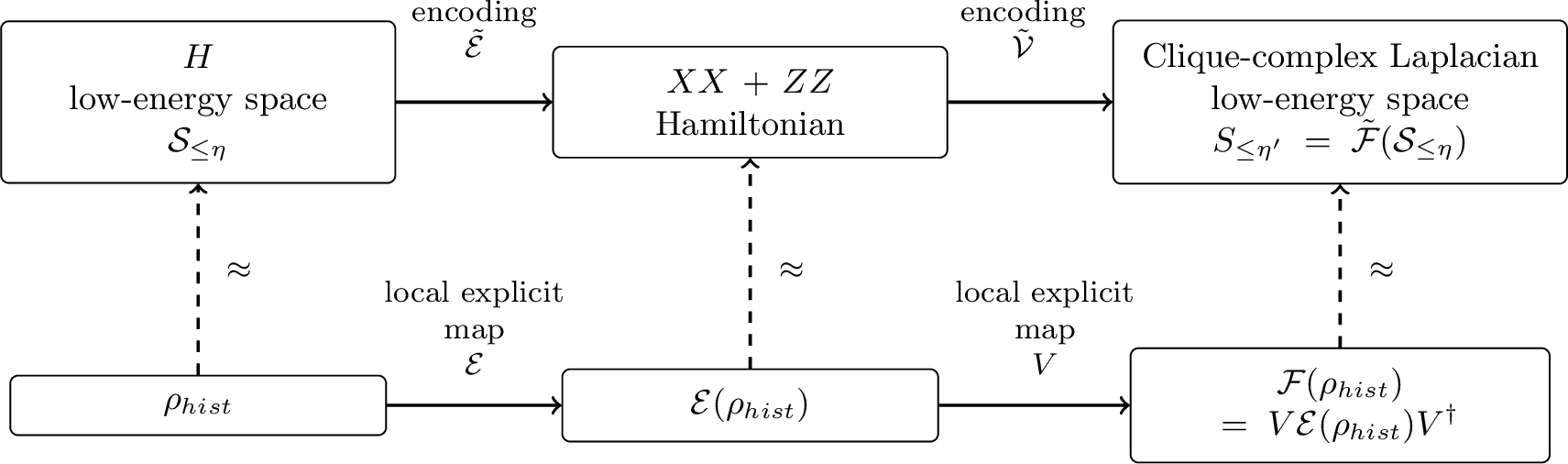
It then follows from Weyl’s inequality that \[|\lambda_i(\Delta_{m-1}) - \lambda_i(H_{\textsf{DQC_1}}) - C| \leq \epsilon/2\] where \(\lambda_i(\Delta_{m-1})\) is the \(i\)’th eigenvalue of \(\Delta_{m-1}(G)\) below \(\Lambda\) (in ascending order not counting multiplicities) and \(\lambda_i(H_{\textsf{DQC_1}})\) denotes the \(i\)’th eigenvalue of \(H_\textsf{DQC_1}\) (also in ascending order). Then we consider an instance of LENS for TDA with the graph \(G\) and threshold \[\eta' = \frac{J_{in}}{2(T+1)}+C+\epsilon_{sim}.\] We also take the precision in this instance to be \(\epsilon/2\) and note that the slightly smaller gap \(\delta':=\delta-2\epsilon_{sim}\geq1/\mathrm{poly}(n)\) satisfies the property that \(\Delta_{m-1}(G)\) has no eigenvalue in \((\eta', \eta'+\delta']\). Let \(\chi\) denote the output of an oracle for this LENS for TDA instance. Then we have \[\label{eqn:32bound32132LENS32hardness} \left| \frac{\sum_{0\leq\lambda_i\leq\eta'}\lambda_i(\Delta_{m-1})}{\dim S_{\leq \eta'}} - \chi\right|\leq \frac{\epsilon}{2}\tag{6}\] We note that the sum over \(\lambda_i(\Delta_{m-1})\) will include the additional multiplicities occurring from the complex to real CMP simulation. However, this just doubles the multiplicities of all eigenvalues, and so the sum as well as the dimension are both doubled which leaves the whole quantity unchanged. In particular, we have that \(\dim S_{\leq \eta'} = 2\dim S_{\leq \eta} = 2\cdot2^{N-1}\), from our choice of \(\eta'\) and since both \(\Delta_{m-1}\) and \(H_\textsf{DQC_1}\) have a spectral gap above these thresholds. Hence, adjusting for the multiplicities we have \[\frac{1}{\dim S_{\leq\eta'}}\sum_{0\leq \lambda_i\leq\eta'}\lambda_i(\Delta_{m-1}) = \frac{1}{2^{N-1}}\sum_{\lambda_i\in E_{\leq\eta'}}\lambda_i(\Delta_{m-1})\] where \(E_{\leq \eta'}\) denotes the set of eigenvalues of \(\Delta_{m-1}\) less than \(\eta'\) with each multiplicity halved (so that it matches that of the original DQC\(_1\) Hamiltonian). We can then bound the difference between the low-energy normalized subtrace of \(\Delta_{m-1}\) (shifted down by \(C\)) and that of \(H_\textsf{DQC_1}\): \[\begin{align} \left|\frac{1}{2^{N-1}}\sum_{\lambda_i\in E_{\leq \eta'}}\lambda_i(\Delta_{m-1}) - C - \frac{1}{2^{N-1}}\sum_{\lambda_i\leq \eta}\lambda_i(H_\textsf{DQC_1})\right| &\leq \frac{1}{2^{N-1}}\sum_{i=1}^{2^{N-1}}|\lambda_i(\Delta_{m-1}) -C-\lambda_i(H_\textsf{DQC_1})|\\ &\leq \frac{1}{2^{N-1}}\sum_{i=1}^{2^{N-1}}\epsilon/2\\ &=\epsilon/2 \label{eqn:32bound32232LENS32hardness} \end{align}\tag{7}\] Finally using the triangle inequality with equations 6 and 7 , we can bound the difference between \(\chi-C\) and the low-energy subtrace of \(H_\textsf{DQC_1}\) \[\left| (\chi -C) - \frac{1}{\dim S_{\leq \eta}}\sum_{\lambda_i\leq\eta}\lambda_i \right|\leq \epsilon\] It follows that an oracle for LENS for TDA, together with polynomial-time classical pre and postprocessing is sufficient to determine an output for LENS with arbitrary inverse polynomial precision. We note the polynomial-time preprocessing is needed to compute the simulating Laplacian graph \(G\) and postprocessing is required to subtract the constant \(C\) from the LENS for TDA output. By the simulation results in [28] and [17] both of these can be done in polynomial time classically. Combining the above with the fact that LENS is DQC\(_1\)-hard, it follows that an oracle for LENS for TDA is sufficient to decide an arbitrary DQC\(_1\) instance with polynomial-time classical pre and postprocessing. Hence we conclude that LENS for TDA is DQC\(_1\)-hard.
The above construction summarized in Figure 2 also preserves the state-preparation condition. The encoding \(\mathcal{E}(\cdot)\) is a tensor product of local isometries, and hence is implementable by a polynomial-size circuit. In the Rayudu simulation, the reference encoding maps each computational basis state \(\ket{x_1\cdots x_m}\) to \(\prod_i S_{i,x_i}\ket{vac}\) in the \(m\)-fermion sector, where each \(S_{i,x_i}\) acts only on the constant-size triangle encoding qubit \(i\). This is again a product of constant-size isometries and is efficiently implementable. Therefore, applying the composed explicit encoding to the efficiently preparable history-state mixture from Lemma 8 prepares the uniform mixture over the explicitly encoded low-energy subspace. ◻
6.2 DQC\(_1\)-hardness of LESD for TDA and NQHP↩︎
The remaining two hardness proofs are much simpler. In fact, the proof of DQC\(_1\)-hardness for LESD for TDA is completely analogous to the reduction from LENS to LESD in the case of local Hamiltonians.
Proof of Theorem 4: LESD for TDA is DQC\(_1\)-hard. The proof of this is identical to the proof that LESD is DQC\(_1\)-hard for local Hamiltonians in Section 5.3. Simply replace \(H\) with \(\Delta_{m-1}\) from the proof that LENS for TDA is DQC\(_1\)-hard and also replace the threshold \(\eta=\frac{J_{in}}{2(T+1)}\) with the shifted threshold on the simulator Laplacian \[\eta' = \frac{J_{in}}{2(T+1)}+C+\epsilon_{sim}\] from the same proof. The state-preparation condition is inherited from the same LENS for TDA hard instance: the uniform mixture over the low-energy subspace \(S_{\leq\eta'}\) of \(\Delta_{m-1}(G)\) is prepared by applying the explicit composed encoding to the history-state mixture from Lemma 8. By choosing the simulation and encoding accuracy sufficiently small compared with the precision used in each LESD for TDA query, this preparation is within the required trace-distance error. ◻
It remains to show that Normalized Quasi-Harmonic Persistence (NQHP) is DQC\(_1\)-hard. We do this by reducing from LESD for TDA, which is DQC\(_1\)-hard by the above.
Proof of Theorem 8: NQHP is DQC\(_1\)-hard. We consider an instance of LESD for TDA with the simulator Laplacian \(\Delta_{m-1}\) of the DQC\(_1\) Hamiltonian \(H_\textsf{DQC_1}\) as in the proof of theorem 2. We consider the same upper threshold of \[\eta' = \frac{J_{in}}{2(T+1)}+C+\epsilon_{sim}\] and let \(\delta'\geq1/\mathrm{poly}(n)\) be the gap from the proof of Theorem 2, so that \(\Delta_{m-1}\) has no eigenvalue in \((\eta', \eta'+\delta']\). Let \(b\leq\eta'\) and \(\xi\leq\delta'/2\) be the other thresholds for the problem instance. Then fixing a precision \(\epsilon = \frac{1}{\mathrm{poly}(n)}\), LESD for TDA gives an output \(\chi\) satisfying: \[\label{eq:lesd} \frac{\sum_{0\leq \lambda_i\leq b}1}{\dim S_{\leq \eta'}}-\epsilon \leq \chi\leq \frac{\sum_{0\leq\lambda_i\leq b+\xi}1}{\dim S_{\leq \eta'}}+\epsilon\tag{8}\] We will show that an oracle for NQHP on a suitable instance can provide an output that also satisfies the above, hence solving the LESD for TDA instance.
To see this take \(G_1=G_2=G\), the graph such that \(\Delta_{m-1}\) simulates \(H_{\textsf{DQC_1}}\) as in the proof of theorem 2 and \(d=m-1\). This choice also preserves the state-preparation condition. Since \(G_1=G_2\) and we will choose \(\hat{\eta}\) inside the spectral gap above \(\eta'\), the initial subspace \(\mathrm{Im}\,\mathcal{P}_{1,\hat{\eta}}\) is exactly \(S_{\leq\eta'}\). Hence its uniform mixture is the same state prepared in the LESD for TDA hard instance. Moreover, for every queried \(b\leq\eta'\) we have \(\mathcal{P}_{2,b}\leq \mathcal{P}_{1,\hat{\eta}}\), so \(\mathcal{P}_{2,b}\Pi_{\mathrm{Im}\mathcal{P}_{1,\hat{\eta}}}\mathcal{P}_{2,b}=\mathcal{P}_{2,b}\) and every nonzero eigenvalue is \(1\). Thus the large overlap condition holds with \(a_{\min}=1\). We want to approximate the quantity in eq. 8 by the output between \[\frac{ \dim \mathrm{Im}\mathcal{P}_{2,b}|_{\mathrm{Im}\mathcal{P}_{1,\hat{\eta}}} }{ \tilde{\beta}^{1}_{d,\hat{\eta}} } \quad\text{and}\quad \frac{ \dim \mathrm{Im}\mathcal{P}_{2,b+\xi}|_{\mathrm{Im}\mathcal{P}_{1,\hat{\eta}}} }{ \tilde{\beta}^{1}_{d,\hat{\eta}} }\] with properly chosen parameters \(\hat{\delta}\) and \(\hat{\eta}\). Clearly, this is achieved if \[\tilde{\beta}^{1}_{d,\hat{\eta}} = \dim S_{\leq \eta'}\] and \[\mathrm{Im}\mathcal{P}_{2,b}|_{\mathrm{Im}\mathcal{P}_{1,\hat{\eta}}} = S_{\leq b}, \quad \text{and}\quad \mathrm{Im}\mathcal{P}_{2,b+\xi}|_{\mathrm{Im}\mathcal{P}_{1,\hat{\eta}}} = S_{\leq b+\xi}\] hold. (In the definition of NQHP, it is required that \(b+\xi\leq \hat{\eta}\) holds for all allowed \(b\).) We take \(\hat{\eta}:=\eta'+\xi\) and \(\hat{\delta}:=\delta'-\xi\). We will see that this choice of parameters satisfies these conditions.
6.2.0.1 Matching the numerator.
Since there is no spectrum in \((\eta',\eta'+\delta']\), we have \(S_{\leq\hat{\eta}}=S_{\leq\eta'}\) and \(b+\xi\leq\hat{\eta}\) for every \(b\leq\eta'\). Taking \(\xi\) and \(\epsilon\) to be the same as in the LESD for TDA instance also we see the following. For any \(b+\xi\leq\hat{\eta}\) we see that \(\mathrm{Im}\mathcal{P}_{2,b}\subset \mathrm{Im}\mathcal{P}_{1,\hat{\eta}}\). This is because \(\mathcal{P}_{1,\hat{\eta}}\) is the orthogonal projector onto the eigenstates of \(\Delta_{m-1}(G_1)\) with eigenvalues less than \(\hat{\eta}\) and \(\mathcal{P}_{2,b}\) is the orthogonal projector onto eigenstates of \(\Delta_{m-1}(G_2)\) with eigenvalue less than \(b\). But since we took \(G_1=G_2\) the two combinatorial Laplacians coincide, and hence the subspace corresponding to eigenvalues below \(b\) is a subset of that for eigenvalues below \(\hat{\eta}\). Immediately this gives: \[\mathrm{Im}\mathcal{P}_{2,b}|_{\mathrm{Im}\mathcal{P}_{1,\hat{\eta}}} = \mathrm{Im}\mathcal{P}_{2,b} = \mathrm{Span}(\{\ket{\psi_i}: \lambda_i\leq b\}) = S_{\leq b}\] The same is also true for the case with \(\xi\) in the numerator threshold. That is \[\mathrm{Im}\mathcal{P}_{2,b+\xi}|_{\mathrm{Im}\mathcal{P}_{1,\hat{\eta}}} = S_{\leq b+\xi}.\]
6.2.0.2 Matching the denominator.
Turning attention to the denominator, we see that by definition \(\tilde{\beta}_{m-1,\hat{\eta}} = \dim S_{\leq \hat{\eta}}=\dim S_{\leq\eta'}\). Hence overall we have \[\frac{\dim \mathrm{Im}\mathcal{P}_{2,b}|_{\mathrm{Im}\mathcal{P}_{1,\hat{\eta}}}}{\tilde{\beta}^1_{d,\hat{\eta}}}= \frac{\dim S_{\leq b}}{\dim S_{\leq \eta'}} = \frac{\sum_{0\leq\lambda_i\leq b}1}{\dim S_{\leq \eta'}}\] as well as the analogous result when \(b\) is replaced with \(b+\xi\). Hence it follows that for any \(b\leq\eta'\), the output of this NQHP instance satisfies the same bounds as the original LESD for TDA instance. Moreover, the proof of DQC\(_1\)-hardness for LESD for TDA only required outputs for \(b\leq\eta'\) with the same choice of \(\eta'\). Hence we conclude that polynomially many queries to an oracle for NQHP is sufficient to decide an arbitrary DQC\(_1\) instance, and so NQHP is DQC\(_1\)-hard by a polynomial-time truth-table reduction. ◻
7 Toward \(\mathsf{SDQC}_1\)-Hardness of NHP↩︎
In this section, we discuss a route toward proving Conjecture 1. First, we explain why the TDA analogue of Normalized Persistence requires a stronger ingredient than the simulation tools used in the proof of Normalized Quasi-Harmonic Persistence. The quasi-harmonic result in Section 6.2 relies on approximate low-energy simulation based on the Rayudu construction, combined with universal Hamiltonian simulation. By contrast, NHP reads the exact harmonic space. A perturbative simulation that moves zero eigenvalues by inverse-polynomial error can preserve all low-energy density estimates used for NQHP, while completely losing the Betti number and hence the persistent Betti number.
The closest existing exact-kernel primitive is the King–Kohler construction for gapped clique homology [15]. This construction performs a reduction from a \(\mathsf{QMA}_1\) verification problem, formulated through a quantum satisfiability instance, to clique homology, while preserving the zero-energy space of the local Hamiltonian and approximately preserving the promise gap for the combinatorial Laplacian. More concretely, they reduce from local Hamiltonians composed of projectors onto integer states, where integer states refer to states with integer amplitudes in the computational basis up to normalization, and construct a clique complex by (1) constructing a qubit graph with \(2^n\) holes and (2) adding gadgets for each local projector with small vertex weights. However, the King–Kohler construction does not give the ingredient needed here as a black box. Our reduction from \(\mathsf{SDQC}_1\) does not merely ask whether a kernel is nonempty. It asks for the dimension of a whole perfectly accepted subspace, normalized by the dimension of the valid history subspace. It also asks that this quotient be reproduced through a filtration. Moreover, the local-Hamiltonian proof in this work uses a hierarchy of penalty scales: the output term is treated as a smaller perturbation relative to the clock, propagation, and input terms. To transfer the proof to clique complexes, one would need a coefficient-sensitive refinement of the King–Kohler construction that represents this relative output weight while preserving the exact kernel and an inverse-polynomial gap.
It is useful to separate the missing proof into an exact-kernel analogue of the route used for NQHP. The natural intermediate problem is a TDA version of LEKD: given a weighted clique complex and a dimension \(d\), estimate the fraction of the relevant low-energy space that is exactly harmonic, with a promise gap above zero. For the \(\mathsf{SDQC}_1\) history Hamiltonian, the corresponding target construction would have two stages. A natural candidate for this step is the circuit-to-Hamiltonian construction of [44], which is better suited to the clique-complex realization. We omit the details of this construction here. First, one would realize the output-free history Hamiltonian \[H_1 := J_{in}H_{in} +J_{prop}H_{prop} +J_{clock}H_{clock}\] by a weighted combinatorial Laplacian \(\Delta_{1,d}\) in such a way that \(\ker\Delta_{1,d}\) has the same dimension as \(\ker H_1\), and the spectral gap above this kernel is preserved up to inverse-polynomial accuracy.
Second, one would add an output gadget corresponding to \[H_2(\lambda) := H_1 + \lambda H_{out},\] where \(\lambda\) is inverse-polynomial but smaller than the scale of the gadgets enforcing the output-free history space. One would assign inverse-polynomially smaller vertex weights to the output gadget than to the gadgets implementing \(H_1\). With this comparatively small output weight, the desired property of the Laplacian \(\Delta_{2,d}\) is \[\dim\ker\Delta_{2,d}=\dim\ker H_2(\lambda),\] with an inverse-polynomial gap above the harmonic space. Establishing this coefficient-sensitive construction along with the approximate preservation of the spectral gap appears to require new control beyond the present King–Kohler analysis.
Finally, NHP needs more than a kernel count for a single simplicial complex. The weighted complexes must form a filtration \(X_1\hookrightarrow X_2\), and the encodings of the kernels must be compatible with this inclusion. Ideally, the filtration should use a common encoding of the valid history space: the chain-level inclusion \(C_d(X_1)\hookrightarrow C_d(X_2)\) should send each encoded history state in \(X_1\) to the same encoded history state in \(X_2\). Under this identification, projecting onto the harmonic space of \(X_2\) should correspond exactly to projecting \(\ker H_1\) onto \(\ker H_2(\lambda)\). Then \[\beta_d(X_1)=\dim\ker H_1, \qquad \beta_d^{1,2}= \dim\mathrm{Im}\,\Pi_{\ker H_2(\lambda)}\big|_{\ker H_1},\] and an oracle for NHP would decide the underlying \(\mathsf{SDQC}_1\) instance in the same way as the local-Hamiltonian Normalized Persistence oracle.
We isolate this missing ingredient as the following conjecture and then show that this conjecture implies Conjecture 1.
Conjecture 2 (Coefficient-sensitive kernel realization). There is a polynomial-time procedure that, given PSD history Hamiltonians that are sums of projectors onto integer states with global coefficients \[H_1= J_{in}H_{in} +J_{prop}H_{prop} +J_{clock}H_{clock}, \qquad H_2(\lambda)=H_1+\lambda H_{out},\] arising from an \(\mathsf{SDQC}_1\) verifier over a fixed gate set, where \(\lambda\) is inverse-polynomially smaller than the gadget scale of \(H_1\), outputs a dimension \(d\) and weighted clique complexes \(X_1\hookrightarrow X_2\) with \(|V(X_i)|,d=\mathrm{poly}(n)\) such that, writing \(\Delta_{i,d}\) for their \(d\)-dimensional combinatorial Laplacians:
(Kernel fidelity and gap) there are isometries \(\mathcal{E}_i\) satisfying \(\ker\Delta_{i,d}=\mathcal{E}_i(\ker H_i)\), where \(H_2\) denotes \(H_2(\lambda)\). In particular, \(\beta_d(X_i)=\dim\ker H_i\). Moreover, the procedure outputs efficiently computable inverse-polynomial lower bounds \(\widehat{\delta}_1,\widehat{\delta}_2 \geq 1/\mathrm{poly}(n)\) such that each \(\Delta_{i,d}\) has no spectrum in \((0,\widehat{\delta}_i]\).
(Functoriality) the encodings are compatible with the simplicial inclusion \(\iota:C_d(X_1)\hookrightarrow C_d(X_2)\) in the following sense: \(\mathcal{E}:=\iota\circ\mathcal{E}_1\) is an isometry on \(\ker H_1\) whose restriction to \(\ker H_2\) agrees with \(\mathcal{E}_2\). Consequently, \[\Pi_{\ker\Delta_{2,d}}\big|_{\ker\Delta_{1,d}} = \mathcal{E} \big(\Pi_{\ker H_2(\lambda)}\big|_{\ker H_1}\big) \mathcal{E}^{\dagger},\] and hence \[\beta_d^{1,2} = \dim\mathrm{Im}\, \Pi_{\ker H_2(\lambda)}\big|_{\ker H_1}.\]
This conjecture is deliberately narrower than a full universal simulation theorem. It only asks for the class of frustration-free history Hamiltonians that arise in the \(\mathsf{SDQC}_1\) reduction, and for the preservation of the exact kernel structure rather than the full spectrum. At the same time, it asks for properties that approximate Hamiltonian simulation does not provide: exact kernel multiplicity and compatibility with a filtration. A stronger and independently interesting direction would be to prove a general kernel-preserving universality theorem for weighted clique Laplacians. Such a theorem would likely imply the realization primitive above, but the present conjecture isolates the more specific structure needed for NHP. It would also be interesting to explore kernel-preserving universality for local Hamiltonians.
Lemma 11 (Conditional hardness of Normalized Harmonic Persistence). Conjecture 2 implies that Normalized Harmonic Persistence is \(\mathsf{SDQC}_1\)-hard.
Proof. Let \(x\) be an \(\mathsf{SDQC}_1\) instance. The local-Hamiltonian reduction for Normalized Persistence constructs \(H_1\) and \(H_2(\lambda)=H_1+\lambda H_{\mathrm{out}}\) so that estimating \[\frac{ \dim\mathrm{Im}\, \Pi_{\ker H_2(\lambda)}\big|_{\ker H_1}}{\dim\ker H_1}\] suffices to decide \(x\). Applying Conjecture 2 gives a filtration \(X_1\hookrightarrow X_2\) and a dimension \(d\) with \(\beta_d^1=\dim\ker H_1\) and \[\beta_d^{1,2} = \dim\mathrm{Im}\, \Pi_{\ker H_2(\lambda)}\big|_{\ker H_1}.\] The computable lower bounds \(\widehat{\delta}_1,\widehat{\delta}_2\) ensure that the resulting NHP instance satisfies the required spectral-gap promise. Therefore \[\frac{\beta_d^{1,2}}{\beta_d^1} = \frac{ \dim\mathrm{Im}\, \Pi_{\ker H_2(\lambda)}\big|_{\ker H_1}}{\dim\ker H_1}.\] A single query to NHP on \((X_1,X_2,d)\) therefore decides the \(\mathsf{SDQC}_1\) instance. The reduction is polynomial-time by the size guarantee in the conjecture. ◻
8 Containment of Low-Energy and Normalized Persistence Problems↩︎
In this section, we provide proofs of containments for the low-energy and normalized persistence problems.
8.1 Containment for Low-Energy Problems↩︎
8.1.0.1 Containment of LENS (Lemma 1)
Proof. By the state-preparation assumption, we can prepare a state \(\tilde{\rho}\) satisfying \(\|\tilde{\rho}-\rho_{\mathcal{S}_{\leq\eta}}\|_1\leq\tau\), where \(\tau\leq \epsilon/(3\max\{1,\|H\|\})\). We then modify the Sparse Uniform Eigenvalue Sampling (SUES) algorithm of [6]. Instead of assuming direct access to \(\rho_{\mathcal{S}_{\leq\eta}}\), we proceed as follows:
Prepare \(\tilde{\rho}\).
Perform phase estimation w.r.t.\(e^{iH}\), with precision and Hamiltonian simulation error chosen so that their sum is at most \(\epsilon/3\).
Measure the energy register to obtain \(\hat{\lambda}\).
For the ideal input \(\rho_{\mathcal{S}_{\leq\eta}} = \frac{1}{\dim\mathcal{S}_{\leq\eta}}\sum_{i:\,\lambda_i\leq\eta} \ket{\psi_i}\bra{\psi_i}\), each eigenvalue \(\lambda_i\leq\eta\) is sampled with probability \(1/\dim\mathcal{S}_{\leq\eta}\), up to the phase-estimation error. The trace-distance error from replacing \(\rho_{\mathcal{S}_{\leq\eta}}\) by \(\tilde{\rho}\) changes the expected sampled energy by at most \(\|H\|\tau\leq\epsilon/3\). Averaging over polynomially many independent repetitions and applying Hoeffding’s inequality gives an estimate within additive error \(\epsilon\) of \[\frac{\sum_{0\leq\lambda_i\leq\eta}\lambda_i}{\dim\mathcal{S}_{\leq\eta}}\] with probability at least \(\mu\). ◻
8.1.0.2 Containment of LESD (Lemma 2)
Proof. Again use the state-preparation assumption to prepare \(\tilde{\rho}\) with \(\|\tilde{\rho}-\rho_{\mathcal{S}_{\leq\eta}}\|_1\leq\tau\), where \(\tau\leq\epsilon/3\). We adapt the eigenvalue counting algorithm of [6] for LLSD to solve LESD. Rather than applying phase estimation to the maximally mixed state \(I/2^n\), we proceed as follows:
Prepare \(\tilde{\rho}\).
Perform phase estimation w.r.t.\(e^{iH}\), with precision and Hamiltonian simulation error chosen so that their sum is less than \(\xi/2\).
Measure the energy register to obtain energy estimate \(\hat{\lambda}\), and record the indicator \(\mathbf{1}[\hat{\lambda} \leq b + \xi/2]\).
For the ideal input \(\rho_{\mathcal{S}_{\leq\eta}}\), all eigenvectors with eigenvalue at most \(b\) are counted, while all eigenvectors with eigenvalue greater than \(b+\xi\) are not counted. Thus the ideal fraction of counted samples lies between \[\frac{\sum_{0\leq\lambda_i\leq b}1}{\dim\mathcal{S}_{\leq\eta}} \quad\text{and}\quad \frac{\sum_{0\leq\lambda_i\leq b+\xi}1}{\dim\mathcal{S}_{\leq\eta}}.\] The trace-distance error from replacing \(\rho_{\mathcal{S}_{\leq\eta}}\) by \(\tilde{\rho}\) changes this probability by at most \(\tau\leq\epsilon/3\). By Hoeffding’s inequality, polynomially many independent repetitions suffice to ensure the sampling error is at most \(2\epsilon/3\), with probability at least \(\mu\). This yields an output \(\chi\) satisfying the conditions in LESD. ◻
8.1.0.3 Containment of LEKD (Lemma 3)
Proof. The proof is the same as the proof of Lemma 2, with the final counting threshold specialized to the kernel. Specifically, we proceed as follows:
Prepare \(\tilde{\rho}\) satisfying \(\|\tilde{\rho}-\rho_{\mathcal{S}_{\leq\eta}}\|_1\leq\tau\) with \(\tau\leq\epsilon/3\), using the state-preparation assumption.
Perform phase estimation w.r.t.\(e^{iH}\), with precision and Hamiltonian simulation error chosen so that their sum is less than \(\delta/2\).
Measure the energy register to obtain energy estimate \(\hat{\lambda}\), and record the indicator \(\mathbf{1}[\hat{\lambda} \leq \delta/2]\).
Since \(H\) has no eigenvalue in \((0,\delta]\), every eigenvalue is either \(0\) or greater than \(\delta\). Therefore, for the ideal input \(\rho_{\mathcal{S}_{\leq\eta}}\), eigenstates with \(\lambda_i=0\) are counted and eigenstates with positive energy are not counted. The trace-distance error from using \(\tilde{\rho}\) changes this probability by at most \(\tau\leq\epsilon/3\). The same trace-distance and sampling bounds as above give an additive-\(\epsilon\) estimate of \[\frac{\sum_{\lambda_i=0}1}{\dim\mathcal{S}_{\leq\eta}}\] with probability at least \(\mu\). ◻
8.2 Containment for Normalized Persistence Problems↩︎
8.2.0.1 Containment of Normalized Quasi-Persistence (Lemma 4)
Proof. Let \(\mathcal{S} = \ker H_1\), \(D = \dim\mathcal{S}\), \(P_- = \mathcal{P}_{2,b}\), \(P_+ = \mathcal{P}_{2,b+\xi}\), and \[m_- := \dim\mathrm{Im}\,P_-|_{\mathcal{S}}, \qquad m_+ := \dim\mathrm{Im}\,P_+|_{\mathcal{S}}.\] The goal is to output a number lying between \(m_-/D-\epsilon\) and \(m_+/D+\epsilon\) with probability at least \(\mu\).
Let \(\{\ket{\psi_j}\}_{j=1}^{D}\) be an orthonormal eigenbasis of \(\Pi_{\mathcal{S}}P_-\Pi_{\mathcal{S}}\) within \(\mathcal{S}\), with eigenvalues \(a_j \in \{0\} \cup [a_{\min},1]\). Then \(m_- = |\{j:a_j>0\}|\). Since \(P_-^2=P_-\) and \(\Pi_{\mathcal{S}}\ket{\psi_j}=\ket{\psi_j}\), \[\|P_-\ket{\psi_j}\|^2 = \braket{\psi_j|P_-|\psi_j} = \braket{\psi_j|\Pi_{\mathcal{S}}P_-\Pi_{\mathcal{S}}|\psi_j} = a_j.\]
Using phase estimation for \(H_2\) with precision \(\xi/4\), followed by thresholding at \(b+\xi/2\), we obtain an efficiently implementable cutoff filter. For simplicity, we first consider an idealized projector given by \(Q=\mathcal{P}_{2,b'}\) for some \(b'\in [b,b+\xi]\). The following analysis holds for any projector \(\mathcal{P}_{2,b'}\) where \(b'\in [b,b+\xi]\). The idealized projector satisfies the operator relation \[P_- \leq Q \leq P_+ .\] Equivalently, \(Q\) accepts every eigenvector of \(H_2\) with eigenvalue at most \(b\) and rejects every eigenvector with eigenvalue larger than \(b+\xi\).
Let \(\lambda_1(Q),\ldots,\lambda_D(Q)\) be the eigenvalues of \(\Pi_{\mathcal{S}}Q\Pi_{\mathcal{S}}\) on \(\mathcal{S}\), arranged in nonincreasing order. Since \(\Pi_{\mathcal{S}}P_-\Pi_{\mathcal{S}} \leq \Pi_{\mathcal{S}}Q\Pi_{\mathcal{S}} \leq \Pi_{\mathcal{S}}P_+\Pi_{\mathcal{S}}\), \(\Pi_{\mathcal{S}}Q\Pi_{\mathcal{S}}\) on \(\mathcal{S}\) has at least \(m_-\) number of eigenvectors with eigenvalue \(\geq a_{\mathrm{min}}\). It may have additional eigenvectors (with arbitrary eigenvalues) but the number of non-zero eigenvalues is bounded by \(m_+\). Write the idealized cutoff as a block-encoding \(U_Q\) of \(Q\) with ancilla register \(a\), satisfying \((I \otimes \bra{0^a})\,U_Q\,(I \otimes \ket{0^a}) = Q\) in the idealized analysis. Write \(P_0 := I_n \otimes \ket{0^a}\bra{0^a}\). Consider the following algorithm:
Algorithm.
Prepare \(\rho_{\mathcal{S}}\).
Apply fixed-point amplitude amplification (FPAA) [45] to \(U_Q\) with lower bound \(\sin\theta_{\min} := \sqrt{a_{\min}}\) and error parameter \(\delta\); this requires \(O(a_{\min}^{-1/2}\log(1/\delta)) = \mathrm{poly}(n)\) queries to \(U_Q\).
Measure the ancilla; record success (\(= \ket{0^a}\)).
Repeat for \(O(\epsilon^{-2}\log(1/(1-\mu)))\) independent trials and output fraction of success.
Analysis. Let \(\{\ket{\varphi_j}\}_{j=1}^{D}\) be an orthonormal eigenbasis of \(\Pi_{\mathcal{S}}Q\Pi_{\mathcal{S}}\) on \(\mathcal{S}\), with corresponding eigenvalues \(\lambda_j(Q)\). Write \(\ket{\phi_j}:=\ket{\varphi_j}\ket{0^a}\) and \(\ket{\phi_j'}:=U_Q\ket{\phi_j}\). We analyze the three cases for each of the eigenvectors:
\(\lambda_j(Q) \geq a_{\min}\): The initial success amplitude \(\|Q\ket{\varphi_j}\| = \sqrt{\lambda_j(Q)} \geq \sin\theta_{\min}\). By the fixed-point property of FPAA [45], the post-amplification success probability satisfies \(p_j \geq 1 - 2\delta\).
\(\lambda_j(Q) = 0\): Since \(Q\ket{\varphi_j} = 0\), we have \(P_0\ket{\phi_j'} = 0\), and a direct computation shows that \(\ket{\phi_j'}\) is a fixed point of the oblivious Grover iterate \(G := -U_Q(I-2P_0)U_Q^{\dagger} (I-2P_0)\). Since FPAA is a polynomial in \(G\), the success probability remains zero.
\(0<\lambda_j(Q)<a_{\min}\): We make no amplification guarantee for this case, but the resulting success probability is still between \(0\) and \(1\).
The average success probability over \(\rho_{\mathcal{S}} = \frac{1}{D}\sum_j \ket{\varphi_j}\bra{\varphi_j}\) satisfies \[p_{\mathrm{succ}} = \frac{1}{D}\sum_j p_j \;\in\; \left[\frac{m_-(1-2\delta)}{D},\;\frac{m_+}{D}\right].\] This is because there are at least \(m_-\) eigenvalues that are amplified with success probability at least \(1-2\delta\) and at most \(m_+\) eigenvalues of \(\Pi_{\mathcal{S}}Q\Pi_{\mathcal{S}}\) are nonzero. We can set \(\delta\leq 1/\exp(n)\) while keeping the FPAA procedure efficient. Then, by applying Hoeffding’s inequality to \(O(\epsilon^{-2}\log(1/(1-\mu)))\) trials, the empirical mean estimates \(p_{\mathrm{succ}}\) to within \(\pm\epsilon/3\) with probability \(\geq \mu\).
In the actual implementation, phase estimation gives a filter whose acceptance probability is at least \(1-\alpha\) on eigenvalues \(\leq b\), at most \(\alpha\) on eigenvalues \(>b+\xi\), and arbitrary on the interval \((b,b+\xi]\). We can choose \(\alpha\) inverse-polynomially small compared with \(\epsilon\) and the polynomial length of the FPAA circuit so that the final success probability changes by at most \(\epsilon/3\). Thus the idealized analysis above continues to give \[p_{\rm succ}\in \left[\frac{m_-(1-2\delta)}{D}-\epsilon/3,\, \frac{m_+}{D}+\epsilon/3\right].\] By taking \(\delta\le \epsilon/6\) and estimating \(p_{\rm succ}\) to additive error \(\epsilon/3\), we have \[\frac{m_-}{D}-\epsilon \le \chi \le \frac{m_+}{D}+\epsilon\] with probability at least \(\mu\). ◻
The remaining containment proofs are similar to the above proof.
8.2.0.2 Containment of Normalized Persistence (Lemma 5)
Proof. Apply the proof of Containment of Normalized Quasi-Persistence (Lemma 4) with \(\mathcal{P} = \Pi_{\ker H_2}\). It remains to show that a block-encoding \(U_{\mathcal{P}}\) of \(\Pi_{\ker H_2}\) can be constructed in polynomial time. By running phase estimation on \(H_2\) with precision \(\delta_2' < \delta_2/4\), we can implement an \(\alpha\)-approximate block-encoding of \(\Pi_{\ker H_2}\) with \(\alpha\) sufficiently small compared with the length of FPAA. Then, a similar analysis to Lemma 4 holds. ◻
8.2.0.3 Containment of Normalized Quasi-Harmonic Persistence (Lemma 6)
Proof. Apply the proof of Containment of Normalized Quasi-Persistence (Lemma 4) with \(\mathcal{S} = \mathrm{Im} \mathcal{P}_{1,\eta}\), \(P_-=\mathcal{P}_{2,b}\), and \(P_+=\mathcal{P}_{2,b+\xi}\). An approximate cutoff block-encoding \(U_Q\) for the window \([b,b+\xi]\), with idealized cutoff satisfying \(\mathcal{P}_{2,b}\leq Q\leq \mathcal{P}_{2,b+\xi}\), is obtained by Hamiltonian simulation of \(\Delta_{2,d}\) followed by phase estimation with threshold \(b+\xi/2\) and precision \(O(\xi)\). Then, a similar analysis to Lemma 4 holds. ◻
8.2.0.4 Containment of Normalized Harmonic Persistence (Lemma 7)
Proof. Apply the proof of Containment of Normalized Persistence (Lemma 5) with \(\mathcal{S} = \mathcal{H}_d^1\) and \(\mathcal{P} = \Pi_{\mathcal{H}_d^2}\). The approximate block-encoding of \(\Pi_{\mathcal{H}_d^2} = \Pi_{\ker\Delta_{2,d}}\) is obtained by phase estimation on \(\Delta_{2,d}\) with precision \(\delta_2' < \delta_2/4\). Then, a similar analysis to Lemma 4 holds. ◻
Acknowledgements↩︎
DL acknowledges funding from UK EPSRC (EP/W032643/1 and EP/Z53318X/1). MSK acknowledges funding from the UK EPSRC through EP/Z53318X/1 and EP/W032643/1, the KIST through Open Innovation fund and the National Research Foundation of Korea grant funded by the Korean government (MSIT) (No. RS-2024-00413957). RH was supported by JST PRESTO Grant Number JPMJPR23F9 and JST ASPIRE Grant Number JPMJAP26A4, Japan.
Author Contributions↩︎
DL and RH conceived the idea and proved the results. RB, MSK acted as supervisors for DL and participated in discussions. All four authors participated in writing the final draft.
9 Combinatorial-Laplacian Simulation↩︎
Here we outline the construction used in [17] to show that estimating the minimum eigenvalue of a combinatorial Laplacian is QMA-hard. This construction uses the representation of the combinatorial Laplacian via the fermion hardcore model. That is, a model where no fermions are allowed to occupy adjacent sites. Precisely, consider a weighted graph \(G=(V,E)\) with weight \(u_i\) on vertex \(i\). Then the fermion hardcore model on \(G\) is given by the Hamiltonian: \[H_G = \sum_{(i,j)\in E}u_iu_j P_ia_i^\dagger a_j P_j + \sum_{i\in V}u_i^2P_i\] where \(a_i^\dagger\) and \(a_i\) are fermionic creation and annihilation operators respectively. The \(P_i\) are projectors that enforce the hardcore constraints of the graph and are given by: \[P_i = \prod_{j| (i,j)\in E}({I}-a_j^\dagger a_j).\] We see that each \(P_i\) projects onto the subspace where there are no fermions adjacent to vertex \(i\). It can be shown that \(H_G\) is a direct sum of the combinatorial Laplacians corresponding to the independence complex of \(G\). In particular the \(k\)’th combinatorial Laplacian of \(\bar{G}\) is given by the restriction of \(H_G\) to the subspace with \((k+1)\) fermions. Rayudu [17] used the fermion hardcore model to show that a combinatorial Laplacian can simulate an \(XX+ZZ\) Hamiltonian. Moreover, since these are universal in the sense of [28] it follows that weighted combinatorial Laplacians are also capable of universal simulation in some sense. First suppose that we want to simulate a Hamiltonian consisting of one term, \(\frac{3}{8}\mu_{i,j}(X_iX_j +Z_iZ_j)\), with \(\mu_{i,j}>0\). Hence we want to simulate a 2 qubit space \(\mathcal{H}_{target}= (\mathbb{C}^2)^{\otimes2}\). Then to encode each qubit we use fermionic states that obey the hardcore restrictions on a triangle, as shown in Figure 3. Note that such states must consist of at most one fermion.
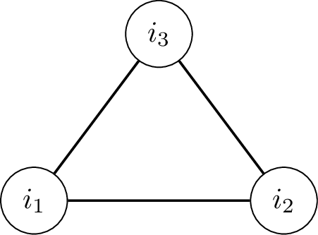
Then consider the fermion hardcore model on this triangle (with coefficients 1 for now) \[H_{0,i} = P_{i_1}a_{i_1}^\dagger a_{i_2}P_{i_2} + P_{i_2}a_{i_2}^\dagger a_{i_1}P_{i_1} + P_{i_1}a_{i_1}^\dagger a_{i_3}P_{i_3} + P_{i_3}a_{i_3}^\dagger a_{i_1}P_{i_1}+ P_{i_2}a_{i_2}^\dagger a_{i_3}P_{i_3} + P_{i_3}a_{i_3}^\dagger a_{i_2}P_{i_2} + P_{i_1} + P_{i_2} + P_{i_3}\] It is clear that the subspace of the Fock space satisfying the hardcore constraints is 4 dimensional, as we cannot have more than one fermion on the graph. One can then show that \(H_{0,i}\) has two \(0\)-energy ground states, given by \[\begin{align} \ket{0}&=S_0\ket{vac}\\ \ket{1}&=S_1\ket{vac} \end{align}\] where \[\begin{align} S_0 &= \frac{1}{2\sqrt{3}}[(1-\sqrt{3})a_3^\dagger - 2a_1^\dagger + (1+\sqrt{3})a_2^\dagger]\\ S_1 &= \frac{1}{2\sqrt{3}}[(1+\sqrt{3})a_3^\dagger -2a_1^\dagger +(1-\sqrt{3})a_2^\dagger] \end{align}\] A 2 dimensional ground space might seem strange, as the complement of this graph has 3 connected components, and so we should expect \(\beta_0=3\). However, the fermion hardcore model instead captures the ‘reduced homology’ of the independence complex. In this convention we consider the empty set (or vacuum in the fermion picture) to be a \((-1)\)-simplex. This means that the \(0\)’th Betti number will now actually be equal to the number of connected components minus one. Note that this convention leaves all other Betti numbers unchanged.
We will use the ground states \(\ket{0},\ket{1}\) to encode qubit \(i\). To encode multiple qubits we use several copies of the same triangle, and the \(XX+ZZ\) interactions between them are simulated using mediator modes \(x,y,z\), see Figure 4.
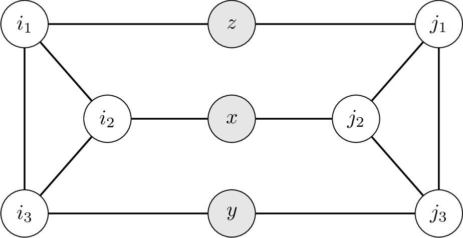
Now consider the Hamiltonian \[H_0 = H_{0,i} + H_{0,j}\] Note that \(H_0\) is just the fermion hardcore model on two disjoint copies of the qubit triangle. It follows that, in the two fermion sector, \(H_0\) has four ground states \[\begin{align} \ket{00} &= S_{0,i}S_{0,j}\ket{vac}\\ \ket{01} &= S_{0,i}S_{1,j}\ket{vac}\\ \ket{10} &= S_{1,i}S_{0,j}\ket{vac}\\ \ket{11} &= S_{1,i}S_{1,j}\ket{vac} \end{align}\] where \(S_{0,i}\) and \(S_{1,i}\) are just the previous \(S_0\) and \(S_1\) operators with all creation operators acting on the \(i\)-nodes. \(S_{0,j}\) and \(S_{1,j}\) are defined analogously. We can then encode the 2 qubit space \(\mathcal{H}_{target} = (\mathbb{C}^2)^{\otimes 2}\) in these ground states. Precisely, we will take the simulator Hilbert space to be \(\mathcal{H}_{sim} = \Pi_{hc}\mathcal{F}^{(2)}\), where \(\mathcal{F}^{(2)}\) denotes the 2 fermion sector of the full fermionic Fock space on the 9 sites, and \(\Pi_{hc}\) is the projector onto states that obey the hardcore constraints corresponding to the graph in Figure 4. That is, \(\mathcal{H}_{sim}\) is the space spanned by states of 2 fermions on the graph in Figure 4 such that no two fermions are adjacent. Importantly, \(\mathcal{H}_{sim}\) does contain states with fermions on the mediators. This means, that for the 2 qubit and 1 interaction graph, \(\dim(\mathcal{H}_{sim}) = 24\). Despite this, the groundspace of \(H_0\) is still 4 dimensional which we use to encode the 2 qubit Hilbert space. The isometry \(\mathcal{E}:\mathcal{H}_{target}\to \mathcal{H}_{sim}\) is then simply the mapping from the 4 computational basis states to the 4 fermionic states above. The goal now is to simulate an \(XX+ZZ\) interaction through a perturbation to \(H_0\) that acts on the mediator modes. This is achieved with the following result of Bravyi and Hastings. Here we assume \(H_0\) has smallest eigenvalue 0 and next smallest eigenvalue greater than or equal to 1. Note that both of these conditions hold for the \(H_0\) defined above. We use \(\Pi_-\) and \(\Pi_+\) to denote the projectors onto the ground space of \(H_0\) and its orthogonal complement, respectively. We also use the standard shorthand \(O_{\pm\pm}\) to denote \(\Pi_{\pm}O\Pi_{\pm}\) for an operator \(O\). With this in mind, the result is as follows:
Theorem 9 (Second Order Simulation [42]). Consider a target Hamiltonian \(H_{target}\) acting on \(\mathcal{H}_{target}\). Suppose there exists an isometry \(\mathcal{E}:\mathcal{H}_{target}\to \mathcal{H}_{sim}\) along with \(H_0\), \(V_{main}\), \(V_{extra}\) acting on \(\mathcal{H}_{sim}\) such that \((V_{main})_{--} = 0\), \(V_{extra}\) is block diagonal with respect to \(\Pi_-\) and \(\Pi_{+}\) and \[\left \lVert \mathcal{E}H_{target}\mathcal{E}^\dagger - (V_{extra})_{--} + (V_{main})_{-+}H_0^{-1}(V_{main})_{+-} \right \rVert\leq \epsilon/2.\] Suppose further that the norms of \(V_{main}\) and \(V_{extra}\) are at most \(\Lambda\). Then \(H_{sim} = \Delta H_0 + \Delta^{1/2}V_{main} + V_{extra}\) simulates \(H_{target}\) (in the sense of Bravyi and Hastings) with an error of \((\eta,\epsilon)\), provided that \(\Delta \geq O(\epsilon^{-2}\Lambda^6 + \eta^{-2}\Lambda^2)\). For the relevant notion of simulation here see definition 6.
The perturbations considered by Rayudu are given by \(V_{main} = \sqrt{\mu_{i,j}}(V_x + V_y + V_z)\) and \(V_{extra} = \mu_{i,j}(P_x + P_y + P_z)\), where \[\begin{align} V_x &= P_xa_x^\dagger a_{i_2}P_{i_2} + P_{i_2}a_{i_2}^\dagger a_x P_x + P_xa_x^\dagger a_{j_2}P_{j_2}+ P_{j_2}a_{j_2}^\dagger a_x P_x\tag{9}\\ V_y &= P_ya_y^\dagger a_{i_3}P_{i_3} + P_{i_3}a_{i_3}^\dagger a_y P_y + P_ya_y^\dagger a_{j_3}P_{j_3}+ P_{j_3}a_{j_3}^\dagger a_y P_y\\ V_z &= P_za_z^\dagger a_{i_1}P_{i_1} + P_{i_1}a_{i_1}^\dagger a_z P_z + P_za_z^\dagger a_{j_1}P_{j_1}+ P_{j_1}a_{j_1}^\dagger a_z P_z. \tag{10} \end{align}\] Aiming to apply the theorem above, we note that \((V_{main})_{--} =0\) since all four ground states of \(H_0\) do not contain a mediator fermion. Then the effect of the perturbation \(V_{main}\) can be computed as \[-(V_{main})_{-+}H_0^{-1}(V_{main})_{+-}= -\frac{7}{12}I + \frac{5}{24}(X_iX_j + Z_iZ_j)\] and similarly the effect due to \(V_{extra}\) is given by \[(V_{extra})_{--} = \frac{4}{3}I + \frac{1}{6}(X_iX_j + Z_iZ_j).\] Note that \(V_{extra}\) is not actually block diagonal with respect to \(\Pi_{-}\) and \(\Pi_{+}\) however this condition in theorem 9 can be relaxed to \((V_{main})_{-+}H_0^{-1}(V_{extra})_{+-}=0\). This is because the block diagonal condition is just to kill three unwanted contributions in the effective Hamiltonian, but the above condition ensures two of these are zero and the third is \(O(\Delta^{-1})\) which can be absorbed into the error. One can then check that this latter condition does hold for our choice of \(V_{extra}\). It remains to upper bound \(\Lambda\), the bound on the operator norms of \(V_{main}\) and \(V_{extra}\). We note that both perturbations consist of projectors, and terms of the form \(Pa^\dagger_pa_qP + Pa_q^\dagger a_pP\), both of which have norm at most one. Hence we have: \[\begin{align} \left \lVert V_{main} \right \rVert &\leq 6\sqrt{\mu_{i,j}}\\ \left \lVert V_{extra} \right \rVert &\leq 3\mu_{i,j} \end{align}\] Hence we can take \(\Lambda = \max\{6\sqrt{\mu_{i,j}}, 3\mu_{i,j}\}\). Putting all of this together we can simulate \[\mu_{i,j}(\frac{3}{4}I + \frac{3}{8}(X_iX_j+Z_iZ_j))\] on the encoded qubits \(i\) and \(j\) with error \((\eta,\epsilon)\) using the simulator Hamiltonian \[H_{sim} = \Delta H_0 + \Delta^{1/2}V_{main}+ V_{extra}\] where we take \(\Delta \geq O(\epsilon^{-2}\Lambda^6 + \eta^{-2}\Lambda^2)\). We note that the target Hamiltonian contains an identity shift from the actual desired Hamiltonian, however since this shift is known the actual spectrum of the desired Hamiltonian can be obtained by subtracting this constant. Finally we see that \(H_{sim}\) is the fermion hardcore model on the graph in Figure 4, with vertex weighting \(u_{i_k}=u_{j_k}=\sqrt{\Delta}\) for \(k=1,2,3\) and \(u_x=u_y=u_z=\sqrt{\mu_{i,j}}\). Since \(\mathcal{H}_{sim}\) is the subspace spanned by two independent fermions, it follows that \(H_{sim}\) is equivalent to \(\Delta_1(\text{ind}(G))\), where \(\text{ind}(G)\) denotes the independence complex of the graph in Figure 4. That is, the first combinatorial Laplacian of the complement graph \(\bar{G}\).
It remains to show how this construction generalises to a full \(n\)-qubit Hamiltonian with XX+ZZ interactions. Let \([n]=\{1,2,\ldots,n\}\) denote the qubits the Hamiltonian acts on, where we have fixed some ordering from 1 to \(n\). Then we denote the set of interactions by \(\mathcal{I}\), where \[\mathcal{I} = \{(i,j)\in [n]^2: i<j \text{and} X_iX_j+Z_iZ_j \text{occurs in}H_{target}\}.\] Motivated by the identity shift in the two qubit case we then take \[H_{target}=CI + \sum_{(i,j)\in \mathcal{I}}\frac{3}{8}\mu_{i,j}(X_iX_j+Z_iZ_j)\] where \(\mu_{i,j} = \mathrm{poly}(n)>0\) and \(C\) is a constant to be determined later. Let \(k = |\mathcal{I}|\leq \frac{n(n-1)}{2}\) also. We will simulate \(H_{target}\) using the fermion hardcore model on a graph. Again we encode each qubit \(i\) using a triangle on the nodes \(i_1,i_2,i_3\) and for each interaction between qubits \(i\) and \(j\) we introduce 3 mediator nodes \(x_{i,j}\), \(y_{i,j}\), \(z_{i,j}\). We do this such that each interaction gives a subgraph identical to the graph in Figure 4. If we call the overall graph constructed in this way \(G\), then it is clear that \(G\) has \(3n+3k\) nodes. We take \(\mathcal{H}_{sim}=\Pi_{hc}\mathcal{F}^{(n)}\), the space spanned by states with \(n\) fermions on \(G\) that satisfy the hardcore constraints. Again, the dimension of \(\mathcal{H}_{sim}\) will be the number of independent sets on \(G\) of size \(n\). Then if we take \[H_0 = \sum_{i=1}^nH_{0,i}\] it is clear that \(H_0\) has a ground space of dimension \(2^n\), spanned by states of the form: \[\begin{align} \ket{00\ldots0} &=S_{1,0}S_{2,0}\cdots S_{n,0}\ket{vac}\\ \ket{10\ldots0}&=S_{1,1}S_{2,0}\cdots S_{n,0}\ket{vac}\\ \ket{01\ldots0}&=S_{1,0}S_{2,1}\cdots S_{n,0}\ket{vac}\\ \ldots \notag \end{align}\] where \(S_{i,0}\) and \(S_{i,1}\) denote the operators \(S_0\) and \(S_1\) with creation operators on the triangle corresponding to \(i\). This ground space is the encoding of the \(n\)-qubit Hilbert space that \(H_{target}\) acts on. Then the perturbations we consider are given by \[\begin{align} V_{main} &= \sum_{(i,j)\in \mathcal{I}}\sqrt{\mu_{i,j}} V_{main}^{(i,j)}\\ V_{extra} &= \sum_{(i,j)\in \mathcal{I}}\mu_{i,j}V^{(i,j)}_{extra} \end{align}\] where \(V_{main}^{(i,j)}=V_{x_{i,j}}+V_{y_{i,j}}+V_{z_{i,j}}\) with each term as in equations (9 10 ) and \(V_{extra}^{(i,j)} = P_{x_{i,j}}+P_{y_{i,j}}+P_{z_{i,j}}\). That is, a sum over all interactions of the same perturbations that we had in the two qubit case. We can then upper bound the norms of the perturbations as \[\begin{align} \left \lVert V_{main} \right \rVert &\leq 6\sum_{(i,j)\in\mathcal{I}}\sqrt{\mu_{i,j}}\\ \left \lVert V_{extra} \right \rVert&\leq 3\sum_{(i,j)\in \mathcal{I}}\mu_{i,j} \end{align}\] and so we can take \[\Lambda = \max\left\{6\sum_{(i,j)\in\mathcal{I}}\sqrt{\mu_{i,j}}, 3\sum_{(i,j)\in\mathcal{I}}\mu_{i,j}\right\}=\mathrm{poly}(n).\] Then one can show with the same computations as before that \[H_{sim} = \Delta H_0 + \Delta^{1/2}V_{main}+ V_{extra}\] is a \((\eta,\epsilon)\) simulation of \(H_{target}\) for \(\Delta \geq O(\epsilon^{-2}\Lambda^6 + \eta^{-2}\Lambda^2)\), by theorem 9. Note that after performing the same computations as the two qubit case, one can see that the identity shift is given by \[C = \frac{3}{4}\sum_{(i,j)\in \mathcal{I}}\mu_{i,j}\] As \(H_{sim}\) acts on the space of \(n\) fermions that satisfy the hardcore constraints, it follows that it is equivalent to the \(\Delta_{n-1}(\text{ind}(G))\), with suitable vertex weighting as in the 2-qubit case. We conclude that an \(n\)-qubit \(XX+ZZ\) Hamiltonian can be simulated (in the sense of Bravyi and Hastings) by the \((n-1)\)’th combinatorial Laplacian of a \(3n+3k\) node graph, up to an efficiently computable identity shift.
10 Formal Statements of Related Problems↩︎
Here we outline some of the related problems that fit into the complexity landscape we discuss. These problems, and their relevant complexities, also appear in Table 1.
First we outline the following problem:
Problem 10 (Normalized Subtrace).
Input:
Real numbers \(\epsilon \geq \frac{1}{\mathrm{poly}(n)}\) and \(1> \mu>1/2\).
A sparse positive semidefinite Hamiltonian \(H \in \mathbb{C}^{2^n\times 2^n}\) with \(\|H\|\leq \mathrm{poly}(n)\).
Output: An estimate \(\chi\in \mathbb{R}\) with probability at least \(\mu\) that satisfies \[\overline{\mathrm{Tr}_\eta}(H) -\epsilon \leq \chi \leq \overline{\mathrm{Tr}_\eta}(H) +\epsilon,\] where \[\overline{\mathrm{Tr}_\eta}(H):= \frac{1}{2^n}\sum_{0\leq \lambda_i \leq \eta} \lambda_i.\]
The following complexity theoretic result was shown in [26].
Theorem 10 ([26]). Normalized Subtrace is DQC\(_1\)-hard for \(O(\log (n))\)-local Hamiltonians.
A related problem was studied in [6]. For a positive semidefinite matrix \(H\in \mathbb{C}^{2^n\times 2^n}\) and \(a\leq b \in \mathbb{R}_{\geq 0}\), we define low-lying spectral density by \[D_H(a,b):=\frac{1}{2^n}\sum_{k:a\leq \lambda_k\leq b} 1,\] where \(\lambda_0 \leq \cdots \leq \lambda_{2^n-1}\) are the eigenvalues of \(H\)1. Then, the Low-lying spectral density estimation (LLSD) problem is defined as follows:
Problem 11 (Low-lying Spectral Density (LLSD) [6]).
Input:
Real numbers \(\epsilon \geq \frac{1}{\mathrm{poly}(n)}\), \(\eta \geq \frac{1}{\mathrm{poly}(n)}\), \(\delta \geq \frac{1}{\mathrm{poly}(n)}\) and \(1> \mu>1/2\).
A sparse positive semidefinite Hamiltonian \(H \in \mathbb{C}^{2^n\times 2^n}\) with \(\|H\|\leq \mathrm{poly}(n)\).
Output: An estimate \(\chi\in [0,1]\) with probability at least \(\mu\) that satisfies \[D_H(0,\eta)-\epsilon \leq \chi \leq D_H(0,\eta+\delta)+\epsilon\]
The following result is known on this problem.
Theorem 11 ([6]). LLSD is DQC\(_1\)-hard for \(O(\log (n))\)-local Hamiltonians.
The two problems above are the inspiration for our problems LENS and LESD. Our results generalise these hardness results such that they still hold when the normalization is taken to be the dimension of a low-energy subspace.
Next, we move to the TDA literature and consider the following problem:
Problem 12 (\(\delta\)-Harmonic Persistence [19]).
- Input:
-
Simplicial complexes \(K_1 \subseteq K_2\), where \(K_i = \mathrm{Cl}(G_i)\) and \(|V(G_i)| = n\) for \(i = 1, 2\).
An integer \(0 \leq p < n\).
A \(\mathrm{poly}(n)\)-size classical description of a set \(S \subseteq K_{1,p}\) of \(p\)-simplices in \(K_1\).
- Promise:
-
Spectral gap \(\gamma(\Delta_p^{K_2}) := \min\{|\lambda| \mid \lambda \in \mathrm{Spec}(\Delta_p^{K_2}),\, \lambda > 0\} \geq \frac{1}{\mathrm{poly}(n)}\).
For the uniform superposition \(\ket{\sigma} := \frac{1}{\sqrt{|S|}}\sum_{\sigma_i \in S}\ket{\sigma_i}\), either
\(\|\mathrm{proj}_{\mathcal{H}_p(K_2)}(\ket{\sigma})\| \geq \delta\), or
\(\|\mathrm{proj}_{\mathcal{H}_p(K_2)}(\ket{\sigma})\| < \frac{1}{\exp(n)}\).
- Output:
-
\(1\) if (a), \(0\) if (b).
This problem was shown to be \(\mathsf{BQP}_1\)-hard and contained in \(\mathsf{BQP}\). The following two promise problems for local Hamiltonians are introduced in [19] as underlying quantum primitives for Harmonic Persistence. First, we introduce the Kernel Overlap problem.
Problem 13 (Kernel Overlap).
Input:
An \(n\)-qubit \(O(\log(n))\)-local Hamiltonian \(H = \sum_{i=1}^m H_i\) with \(m = O(\mathrm{poly}(n))\).
A succinct description of a quantum state \(|\psi\rangle\).
Promise:
Spectral gap \(\gamma(H) := \min\{|\lambda| \mid \lambda \in \mathrm{Spec}(H),\, \lambda > 0\} \geq \frac{1}{\mathrm{poly}(n)}\).
Either (a) \(\|\mathrm{proj}_{\ker H}(|\psi\rangle)\| \geq \frac{1}{\mathrm{poly}(n)}\), or (b) \(\|\mathrm{proj}_{\ker H}(|\psi\rangle)\| < \frac{1}{\exp(n)}\).
Output: \(1\) if (a), \(0\) if (b).
Similarly to the Harmonic persistence, this problem was shown to be \(\mathsf{BQP}_1\)-hard and contained in \(\mathsf{BQP}\) in [19]. Next, we introduce a low-energy variant of this problem.
Problem 14 (Low-energy Overlap). Input:
An \(n\)-qubit log-local Hamiltonian \(H = \sum_{i=1}^m H_i\) with \(m = O(\mathrm{poly}(n))\).
A threshold \(\eta \in \Omega(1/\mathrm{poly}(n))\).
A succinct description of a quantum state \(|\psi\rangle\).
Promise: Either (a) \[\|\mathrm{proj}_{E_{\leq\eta}(H)}(|\psi\rangle)\| \geq \frac{1}{\mathrm{poly}(n)},\] or (b) \[\|\mathrm{proj}_{E_{\leq\eta}(H)}(|\psi\rangle)\| < \frac{1}{\exp(n)}.\]
Output: \(1\) if (a), \(0\) if (b).
Here \[E_{\leq\eta}(H) := \mathrm{Span}_{\mathbb{C}} \left\{ |\psi\rangle \,\middle|\, |\psi\rangle \text{ is an eigenvector of } H \text{ with eigenvalue } < \eta \right\}.\]
This problem is known to be \(\mathsf{BQP}\)-complete [19].