A Decomposable Probe for Few-Step Diffusion Models:
Prompt, Latent, and Score Selectivity across Backbone Families and Distillation Paradigms
July 03, 2026
Abstract
Few-step distilled diffusion students cut text-to-image inference from \(\sim\!50\) to \(1\)–\(8\) network evaluations, but the resulting quality gap is almost always summarised by a single end-to-end FID/CLIP scalar that cannot say which axis of the conditioning response changed, nor whether a behaviour is a property of the architecture, the distillation objective, or simply of being a diffusion model. We replace the scalar with a decomposable probe that injects controlled perturbations along three layers (prompt encoder, denoiser input, denoiser output) under three modes (mean, variance, scale) and six strengths, and reports a bootstrap-median Bures \(W_2^2\) selectivity ratio on Inception features. Applied under a single matched estimator to a sweep of \(23\) models — five teachers and \(18\) distilled students across five backbone families (SDXL, SD1.5, SD3.5, PixArt-\(\alpha\), FLUX), three architecture classes (UNet, DiT, MMDiT), and five distillation paradigms — the three layers read three empirically separable factors: the prompt layer is a universal prompt-mean response within this diffusion T2I sweep (a sanity channel rather than a discriminator), the latent layer reads the prediction type, and the score layer reads the distillation objective. Our main result is that, within this sweep, the latent layer is a near-binary detector of rectified-flow backbones: its ratio exceeds \(1\) across a sustained low-to-mid band only for rectified-flow models (SD3.5, FLUX) and no \(\epsilon\)-prediction model satisfies the sustained-band criterion; the obvious wide-T5-conditioning explanation is ruled out by a matched \(\epsilon\)-prediction control (PixArt-\(\alpha\)), and the fingerprint survives adversarial (ADD) distillation on two RF backbone families as both teacher and student. Two secondary score-layer findings hold across families under narrower scopes: a canonical \(4\)-step Turbo-family ADD-vs-rest contrast (the ADD student is the lowest same-family student at the \(4\)-step comparison on the two UNet families that have a non-ADD baseline — not extrapolated to \(1\)-step, where aggressive non-ADD students can enter the ADD range; the two rectified-flow families contribute ADD-only points consistent with the low-ADD end but without a same-family non-ADD contrast), and a CI-separated trajectory-rollout early-strength score spike observed on both UNet and DiT, with magnitude depending on step count and backbone. All ratios are CI-citable under one estimator; we release the per-cell tables and the estimator.
1 Introduction↩︎
Few-step distilled diffusion students — ADD/Turbo, Lightning, LCM, DMD2, Hyper-SD, and their kin — have collapsed text-to-image inference from \(\sim\!50\) network function evaluations down to \(1\)–\(8\). The price of this speedup is well documented in aggregate (worse FID, weaker prompt alignment, reduced sample diversity), but is reported almost exclusively as a single end-to-end scalar that treats the student as a black box. Such a scalar cannot distinguish a student that has lost prompt-mean sensitivity from one whose latent or score response has changed, nor can it say whether a given behaviour is a property of the architecture, the distillation objective, or simply of being a diffusion model at all. These are mechanistically distinct properties, and a headline number cannot tell them apart.
We take the opposite approach: instead of one scalar, a decomposable probe. Our diagnostic injects controlled perturbations into the forward pass along three orthogonal layers — the prompt encoder, the denoiser input (latent), and the denoiser output (score) — under three modes (mean, variance, scale) and six strengths, and summarises each cell of the resulting grid by a bootstrap-median Bures \(W_2^2\) selectivity ratio on Inception features. The probe is training-free, acts through forward hooks, and is backbone-agnostic.
1.0.0.1 The three layers read three empirically separable factors.
Applied under a single matched estimator to a sweep of \(23\) models — five teachers and \(18\) distilled students, spanning five backbone families (SDXL, SD1.5, SD3.5, PixArt-\(\alpha\), FLUX), three architecture classes (UNet, DiT, MMDiT), and five distillation paradigms — the three layers turn out to be far from redundant. Each reads a distinct, empirically separable property of the model (we use “orthogonal” descriptively throughout, not as a claim of statistical independence): the prompt layer is a universal prompt-mean response within this diffusion T2I sweep (every model is prompt-mean selective and so it discriminates none of our factors of interest, making it a sanity channel rather than a discriminator); the latent layer is a near-binary detector of the prediction type (rectified-flow vs \(\epsilon\)-prediction); and the score layer reads the distillation objective. This decomposition is the spine of the paper and the lens through which we read three findings.
1.0.0.2 Finding 1 (main): the latent layer detects rectified-flow, and the fingerprint survives ADD distillation.
The latent layer shows a sustained low-to-mid-strength elevation (\(R\) above \(1\) across a band of strengths) only for the two rectified-flow backbones (SD3.5, FLUX); \(\epsilon\)-prediction models either stay below \(1\) or show only isolated, non-band-shaped excursions. A control disambiguates the cause: PixArt-\(\alpha\) shares SD3.5’s wide T5 conditioning but is \(\epsilon\)-prediction, and it does not reproduce the band, ruling out the obvious wide-T5-conditioning explanation and attributing the effect to the rectified-flow denoiser. The fingerprint moreover survives distillation: the two distilled students on RF backbones — both pure-adversarial (ADD), an objective that flattens the score-layer signal — still pass on the latent layer. Within this sweep the latent layer is thus a near-binary detector of the prediction type (read as a sustained low-to-mid band) that survives ADD distillation, seen across two RF backbone families (MMDiT and DiT), as both teacher and student.
1.0.0.3 Finding 2: a score-layer ADD-vs-rest detector.
On the score layer at the canonical strength \(s\!=\!0.5\), and at the canonical \(4\)-step comparison, the adversarial-distilled (ADD) student is the lowest of its family, below every \(4\)-step non-ADD student with non-overlapping confidence intervals on both UNet families that contain one; the two non-UNet ADD students extend the low-ADD end to MMDiT and DiT. We state this as a binary contrast at the \(4\)-step comparison and explicitly not as a five-paradigm ranking: the four non-ADD paradigms are not pairwise separable at this cell, and this should not be extrapolated to \(1\) step, where the most aggressive non-ADD students can enter or even undercut the ADD range (SDXL Hyper-1 \(0.35\) below Turbo-1 \(0.49\)).
1.0.0.4 Finding 3: a trajectory-rollout early-strength score spike.
Students whose loss includes a multi-step trajectory-rollout regression term, without a dominant adversarial component, exhibit a localized early-strength spike on the score layer: the low-strength peak (\(s\!\leq\!0.1\)) has a confidence interval strictly above \(1\) and CI-separated above the value at \(s\!=\!0.5\). This appears for consistency (LCM) and backward-simulation (Flash) students on UNet and most strongly for LCM on a pure DiT backbone, while the DiT/MMDiT ADD controls (SD3.5-Turbo, FLUX-schnell) show no such spike. The spike is associated with trajectory-rollout objectives and observed on both UNet and DiT, but its appearance and magnitude depend on step count and backbone.
1.0.0.5 Scope.
This paper is an instrument and its readings. We report the probe and what it reveals across the sweep; we do not attach a downstream task (e.g.model attribution or a training-time correction) here, and we are deliberate about the limits of each reading — the score-layer finding is a binary detector, not a paradigm ranking. We release all per-cell CI-citable tables and the matched estimator.
1.0.0.6 Contributions.
A decomposable layer-/mode-resolved probe for diffusion text-to-image models, with a bootstrap-median true Bures \(W_2^2\) selectivity ratio and a single matched estimator applied identically to \(23\) models.
A separable-factor decomposition: across five families and three architecture classes, the prompt / latent / score layers read a universal property / the prediction type / the distillation objective, respectively.
A rectified-flow detector: within this sweep the latent layer is a near-binary detector of the prediction type (read as a sustained low-to-mid band) that survives ADD distillation, with the obvious wide-T5-conditioning explanation ruled out by a matched \(\epsilon\)-prediction control and four RF cases spanning two architecture families and teacher/student roles.
Two cross-family score-layer findings: a canonical \(4\)-step Turbo-family ADD-vs-rest contrast (ADD lowest same-family student at the \(4\)-step comparison on the two UNet families, not extrapolated to \(1\)-step, with ADD-only points extending it to the two RF families), and a trajectory-rollout early-strength spike present on both UNet and DiT.
2 Related Work↩︎
2.1 Few-Step Diffusion Distillation↩︎
Recent years have produced a dense menu of methods that compress multi-step diffusion teachers (\(20\)–\(50\) sampler steps) [1], [2] into 1–8-step students. We group them by the distillation loss family, since this taxonomy is the backbone of our experimental design rather than a survey end-point: (a) Adversarial Diffusion Distillation (ADD) [3] and its progressive variant SDXL-Lightning [4] train the student against an adversarial discriminator and a teacher-derived score loss; (b) Consistency Models [5], [6] and their latent-space adaptations LCM and LCM-LoRA [7], [8] train the student to be self-consistent along the diffusion trajectory; (c) Score Identity / Distribution Matching Distillation (SiD, DMD, DMD2) [9]–[11] reformulate the distillation objective as an identity over scores or as a distribution-matching loss with an auxiliary fake-score network; (d) Trajectory-segmented hybrids such as Hyper-SD [12] interleave consistency, score, and adversarial objectives on partitioned timestep ranges; and (e) Backward simulation approaches like Imagine Flash [13] and Flash Diffusion [14] feed student trajectories back into the training loop. Our sweep instantiates these families on non-UNet backbones as well — SD3.5-Turbo (ADD on MMDiT, [15], [16]), FLUX.1-schnell (ADD on DiT, [17], [18]), and PixArt-LCM (consistency on DiT, [7], [19], [20]) — which is what lets the probe’s readings be tested off the UNet backbone.
Table 1 uses short operational paradigm labels that map onto these families: ADD (a) covers both the Turbo-family adversarial objective (SD-Turbo, SDXL-Turbo) and the progressive-adversarial variant SDXL-Lightning [4] — which builds on the progressive-distillation lineage [21] but adds an adversarial objective — and which we label progressive-adv to distinguish it from the Turbo-family ADD variant; trajectory denotes the consistency family (b) (LCM); distribution-match (c); mixed denotes the trajectory-segmented hybrid Hyper-SD (d); and Flash Diffusion (e) is a backward-simulation objective, labelled backward-sim. We use the term trajectory-rollout operationally in Section 4.5 for objectives that train on student or generated trajectory segments — the consistency (b) and backward-simulation (e) families — even when combined with auxiliary adversarial terms, and reserve ADD for the adversarial-dominant objectives (a).
2.2 Architectures and Prediction Types↩︎
Our sweep spans three architecture classes that differ along two axes relevant to the probe: the backbone family and the denoiser prediction type. (i) UNet with \(\epsilon\)-prediction: SDXL [22] (two CLIP [23] text encoders) and SD1.5 (one CLIP encoder) are the classical latent-diffusion [24] configuration. (ii) Diffusion Transformer (DiT) with \(\epsilon\)-prediction: PixArt-\(\alpha\) [19] replaces the UNet with a pure transformer [25] and conditions on a single T5-XXL [26] encoder, holding the wide T5 conditioning of the rectified-flow models fixed while keeping \(\epsilon\)-prediction — which is exactly what lets it serve as the control that isolates the prediction type in Section 4.3. (iii) Rectified-flow denoisers: SD3.5 (an MMDiT with two CLIP encoders plus T5, [15]) and FLUX [17] (a DiT with CLIP-L plus T5)2 are trained under a flow-matching / rectified-flow objective [27], [28] rather than \(\epsilon\)-prediction. The prediction-type axis (rectified-flow vs \(\epsilon\)-prediction) is the one the latent layer turns out to read.
2.3 CFG Geometry in Multistep Diffusion↩︎
A separate thread analyses the geometry of classifier-free guidance (CFG, [29]) and its effect on sample diversity. [30] show that CFG behaves as a predictor–corrector on the score, alternating a denoising predictor with a sharpening corrector in the SDE limit, and [31] disentangle quality from variation by guiding generation with a weaker version of the same model (autoguidance) rather than with an unconditional one. These analyses are multi-step and live in the limit of large NFE. Our setting differs in two respects: we operate on distilled few-step students (1–8 NFE) and we measure response geometry on real Inception features rather than in an analytical large-NFE limit.
2.4 Inference-Time / Test-Time Interventions↩︎
A group of methods modifies inference without altering diffusion weights. PAG (perturbed-attention guidance, [32]) replaces self-attention with identity in a guidance branch; FreeU [33] reweights the U-Net backbone features while suppressing low-frequency skip-connection components; AYS (align-your-steps, [34]) reshapes the timestep schedule under a KL-optimality criterion. We relate to this line methodologically: like these methods our probe acts through forward hooks and needs no retraining, but it is a diagnostic instrument that reads model behaviour rather than an intervention that changes it.
2.5 Diagnostic Metrics for Generative Models↩︎
The metric stack we use is standard but combined deliberately around one design choice the related literature does not commit to: a bootstrap-median Bures \(W_2^2\) ratio as the headline statistic.
The full closed-form Gaussian \(W_2^2\) on Inception features is the natural feature-space distance under our setup but is non-linear in the empirical covariance, so the plug-in estimator does not coincide with the bootstrap distribution of the same functional at our cell sizes (cf.Section 3.1). We therefore report a bootstrap-median ratio with the full Bures \(W_2^2\) functional inside the bootstrap loop; the bootstrap-median aligns the point estimate and its confidence interval under a single statistical object. Larger-scale alternatives such as Sinkhorn–\(W_2\) [35] could be substituted without changing the qualitative conclusions. We read single-number FID with care, since it is a biased estimator whose bias depends on the model and sample size [36], [37]; our headline statistic is therefore the bootstrap-median ratio rather than a raw plug-in FID. A \(W_2^2\)-independent diversity channel (e.g.a Vendi score [38] on DINOv2 [39] embeddings, which does not share the Bures functional with our headline ratio) is a natural complement to the probe; we leave a full diversity readout to future work.
3 The Probe↩︎
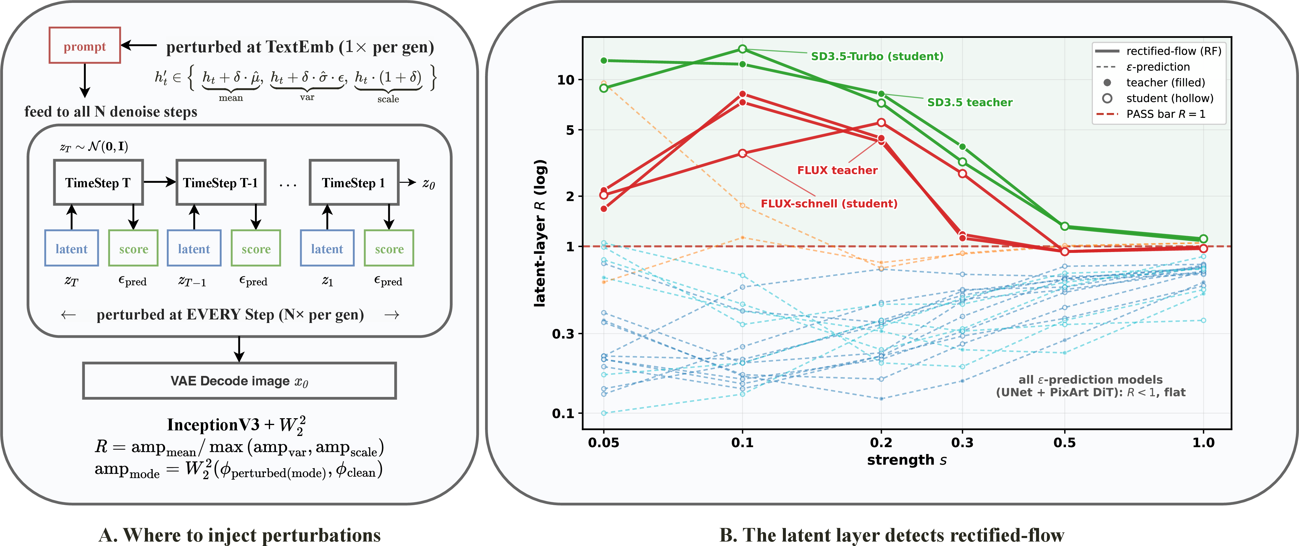
We probe a diffusion text-to-image model by injecting controlled perturbations into its forward pass and measuring how the output distribution responds. The probe is deliberately decomposable: it factors the response along three injection layers and three perturbation modes, and (Section 4.2) each layer turns out to read a different, orthogonal property of the model.
3.1 Layer–Mode Selectivity Scan↩︎
3.1.0.1 Setup.
Given a diffusion model \(G_\theta\) (teacher or distilled student), we inject controlled perturbations along three orthogonal layers and measure how the output distribution responds. The three layers are:
Prompt layer (\(\mathcal{P}_\text{prompt}\)): forward hook on the text-encoder hidden states (one site per encoder; backbones expose 1–3 text encoders, see Section 4.1).
Latent layer (\(\mathcal{P}_\text{latent}\)): forward pre-hook on the denoiser input (UNet for SDXL/SD1.5; the DiT/MMDiT
transformerfor PixArt/SD3.5/FLUX).Score layer (\(\mathcal{P}_\text{score}\)): forward hook on the denoiser output (the predicted \(\epsilon\)/velocity).
On each layer we apply three perturbation modes of strength \(s\): mean (\(x \mapsto x + s\hat{\mu}\)), variance (\(x \mapsto x + s\hat{\sigma}\,\varepsilon\), \(\varepsilon\sim\mathcal{N}(0,I)\)), and scale (\(x \mapsto (1+s)x\)), where \(\hat{\mu},\hat{\sigma}\) are estimated on a calibration set. The full grid is \(3\,\text{layers}\times 3\,\text{modes}\times 6\,\text{strengths}\) with \(s\in\{0.05,0.1,0.2,0.3,0.5,1.0\}\).
3.1.0.2 Selectivity ratio.
For each (layer, strength) cell, let \(\mathrm{amp}_m \;=\; W_2^2\!\bigl(\phi(G_\theta(\cdot;\,\mathrm{perturb}_m)),\,\phi(G_\theta(\cdot))\bigr)\) denote the squared \(W_2\) distance between perturbed and clean Inception-v3 [40] features \(\phi\), evaluated under perturbation mode \(m\in\{\text{mean},\text{var},\text{scale}\}\). Each \(\mathrm{amp}_m\) is computed using the full Bures \(W_2^2\) functional [41] on \(d\!=\!2048\) Inception-v3 features, evaluated within a bootstrap-median framework (Section 2.5). We summarise the cell by the selectivity ratio \[\label{eq:ratio} R_\text{sel} \;=\; \frac{\mathrm{amp}_\text{mean}}{\max(\mathrm{amp}_\text{var},\,\mathrm{amp}_\text{scale})},\tag{1}\] which is large iff the mean perturbation dominates both higher-moment perturbations on that layer. We compute a bootstrap percentile interval over \(n\) resamples of the prompt set and report the \(5\text{th}, 50\text{th}, 95\text{th}\) percentiles as \(R_\text{lo}, R_\text{point}, R_\text{hi}\) respectively, i.e.a \(90\%\) percentile interval centred on the bootstrap median.
3.1.0.3 Why bootstrap-median rather than plug-in.
At our operating cell sizes (\(n\!\approx\!1500\)–\(2000\) prompts, \(d\!=\!2048\) Inception features) the plug-in \(R_\text{sel}\!=\!\widehat{W_2^2}(\text{base},\text{mean})/\max\widehat{W_2^2}(\text{base},\{\text{var},\text{scale}\})\) inherits a non-linear functional bias: the Bures functional is non-linear in the covariance and the bias does not cancel between numerator and denominator, so the plug-in \(R_\text{sel}\) does not match the bootstrap distribution of the same ratio. Reporting the bootstrap-median percentiles therefore aligns the headline point and its interval under a single statistical object; the plug-in value is retained in our release for audit. A formal bias decomposition and the audit cells we use to verify the correction are reported in Appendix 7.
3.1.0.4 Reading a cell.
Rather than a binary PASS/NOT-PASS verdict, we report the continuous ratio \(R_\text{point}\) with its \([R_\text{lo},R_\text{hi}]\) interval and the dominant mode, and compare cells
across models under a single matched estimator. Three distinct uses of the ratio recur and should not be conflated. (i) \(R\!=\!1\) is the equality line: the value at which the mean perturbation exactly matches the
strongest higher-moment perturbation on that layer, used only as a reference boundary, not a detector. (ii) The rectified-flow latent detector (Section 4.3) is a sustained-band criterion: a
model/configuration passes when its latent-layer ratios have \(R_\text{lo}\!>\!1\) on at least three of the four low-to-mid strengths \(s\!\in\!\{0.05,0.1,0.2,0.3\}\), including at least
one \(s\!\geq\!0.2\); this is what separates a genuine band from an isolated single-cell low-\(s\) excursion. (iii) The bar \(R_\text{lo}\!\geq\!2.0\) with
dominant mode mean is a conservative strong-selectivity visual marker only, not the detector threshold. The analysis in Section 4 turns on the relative ordering of CI-disjoint ratios and on the
sustained-band criterion, not on the \(R_\text{lo}\!\geq\!2.0\) marker. All reported intervals quantify prompt-resampling uncertainty under a fixed checkpoint, sampler, and generation seed; unless explicitly noted they
should not be read as full cross-seed uncertainty intervals, and they do not include checkpoint-training or generation-seed variability. Intervals narrower than \(0.005\) round to a single value at two decimal places and
are printed as e.g.\(0.66\,[0.66,0.66]\).3 We do not read isolated cells as discoveries. The main claims are restricted to structured
contrasts stated in advance — sustained bands across adjacent strengths, matched-step same-family contrasts, and CI-separated low-strength peaks — and we apply no family-wise multiple-comparison correction; the released grid should be read as exploratory
outside these stated contrasts.
3.2 Matched Estimator across the Sweep↩︎
Every ratio reported in this paper comes from a single two-stage pipeline applied identically to all 23 models. Stage A computes per-cell true Bures \(W_2^2\) point estimates from an \(n_\text{base}\)-prompt conditioning bank against per-strength perturbed banks of the same size. Stage B (GPU float64) bootstraps \(n_\text{resample}\!=\!200\) true Bures \(W_2^2\) ratios per cell, replaces the point with the bootstrap median, and records the \(5/95\)th percentile interval, so point and CI come from one coherent distribution. Holding the estimator
fixed across SDXL, SD1.5, SD3.5, PixArt-\(\alpha\), and FLUX is what makes the cross-backbone ratios directly comparable. A faster diagonal-covariance proxy used for early sweeps is biased relative to the true Bures
estimator and is never used for a main-text claim; the bias analysis and audit trail are in Appendix 7.
4 Experiments↩︎
4.1 Experimental Setup↩︎
4.1.0.1 The 23-model sweep.
We run the probe on a sweep of \(23\) models, all measured under the identical matched estimator of Section 3.2: five teachers and \(18\) distilled students, spanning five backbone families, three architecture classes (UNet, DiT, MMDiT), and five distillation paradigms. We count a model as a checkpoint with a fixed sampler step setting, so student step variants (e.g.Hyper at \(1/4/8\) steps) count separately; FLUX.1-dev is one checkpoint evaluated at both \(28\) and \(50\) steps and counted once. Table 1 lists the full set. The design is a stress test: a layer reading is only an instrument if it tracks the same factor across families, prediction types, paradigms, and step counts rather than an artefact of any single configuration.
| Family | Arch.class | Text enc. | Role | Paradigm | Steps |
|---|---|---|---|---|---|
| SDXL | UNet | 2\(\times\)CLIP | teacher | — | 50 |
| SDXL | UNet | 2\(\times\)CLIP | student | distribution-match. | 1, 4 |
| SDXL | UNet | 2\(\times\)CLIP | student | mixed (Hyper) | 1, 4, 8 |
| SDXL | UNet | 2\(\times\)CLIP | student | trajectory (LCM) | 4, 8 |
| SDXL | UNet | 2\(\times\)CLIP | student | progressive-adv | 4 |
| SDXL | UNet | 2\(\times\)CLIP | student | ADD (Turbo) | 1, 4 |
| SD1.5 | UNet | 1\(\times\)CLIP | teacher | — | 50 |
| SD1.5 | UNet | 1\(\times\)CLIP | student | trajectory (LCM) | 4 |
| SD1.5 | UNet | 1\(\times\)CLIP | student | backward-sim (Flash) | 4 |
| SD1.5 | UNet | 1\(\times\)CLIP | student | mixed (Hyper) | 4 |
| SD1.5 | UNet | 1\(\times\)CLIP | student | ADD (SD-Turbo) | 1, 4 |
| PixArt-\(\alpha\) | DiT, \(\epsilon\)-pred | T5 | teacher | — | 20 |
| PixArt-\(\alpha\) | DiT, \(\epsilon\)-pred | T5 | student | trajectory (LCM) | 4 |
| SD3.5 | MMDiT, rect.-flow | 2\(\times\)CLIP + T5 | teacher | — | 28 |
| SD3.5 | MMDiT, rect.-flow | 2\(\times\)CLIP + T5 | student | ADD (Turbo) | 4 |
| FLUX.1-dev | DiT, rect.-flow | CLIP-L + T5 | teacher | — | 28, 50 |
| FLUX.1 | DiT, rect.-flow | CLIP-L + T5 | student | ADD (schnell) | 4 |
4pt
4.1.0.2 Prompts and metrics.
Unless stated otherwise, measurements start from \(2{,}000\) MS-COCO [42] val captions, fixed across all cells of the perturbation grid (SD1.5 and SDXL at \(512^2\); SD3.5, PixArt-\(\alpha\), and FLUX at \(1024^2\)). After discarding generations that fail to decode or produce degenerate features, the effective per-cell bank is \(n\!\approx\!1500\)–\(2000\) prompts (Section 3.1), held fixed within a model. Image features are Inception-v3 [40] pool3 (\(2048\)-d); the \(W_2^2\) distance is the closed-form Bures functional [41] under a Gaussian assumption on Inception features. Bootstrap CIs use the matched estimator of Section 3.2 (\(n_\text{resample}\!=\!200\), base-fixed).
4.2 The Three Layers Read Three Orthogonal Factors↩︎
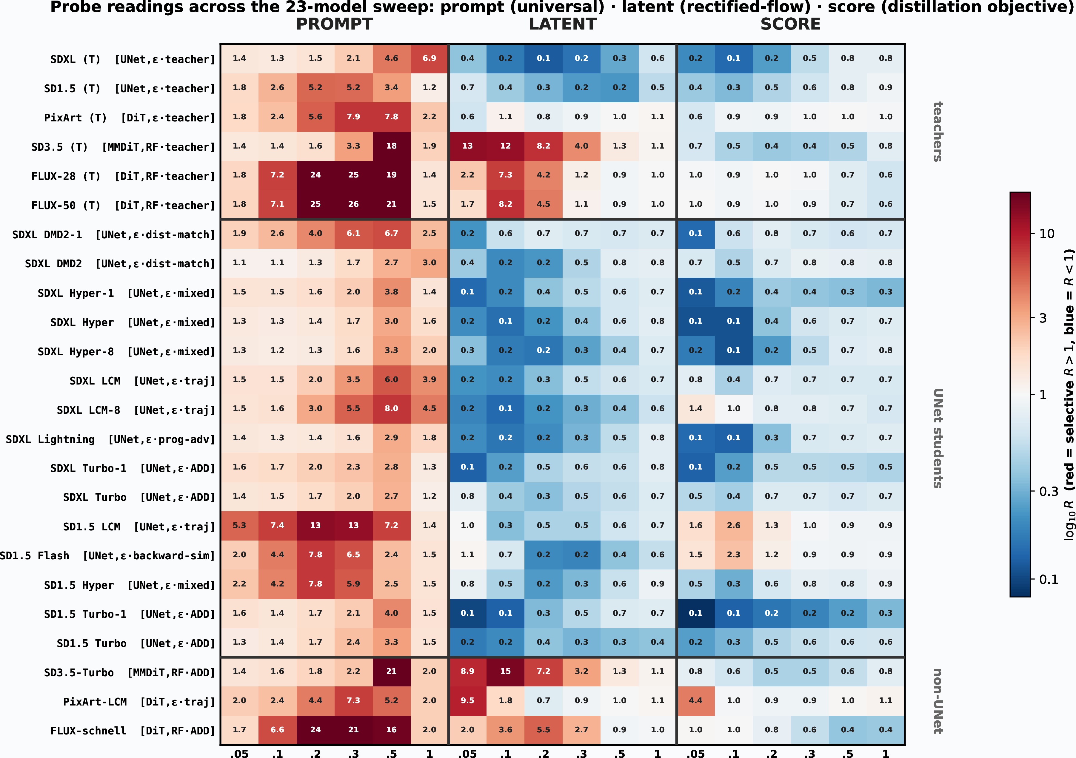
The central empirical observation of the paper is that the three injection layers are not three noisy views of one quantity; each tracks a distinct, empirically separable property of the model (Figure 2). Table 2 summarises the partition that holds across all \(23\) models.
| Layer | Factor it reads | Signature across the 23-model sweep |
|---|---|---|
| prompt | common prompt-conditioning | Prompt-mean selective on every model (teacher and |
| response (universal here) | student, all five families); peak ratio varies widely | |
| (\(\sim\!2.7\)–\(26\)) and tracks no factor of interest. | ||
| latent | prediction type | Sustained low-strength elevation (\(R\!>\!1\) across a band) |
| (rectified-flow vs \(\epsilon\)-pred) | only on rectified-flow denoisers; \(\epsilon\)-pred models | |
| lack the band. | ||
| score | distillation objective | ADD students are the lowest same-family student at the |
| (ADD vs non-ADD) | canonical \(4\)-step comparison; trajectory-rollout students spike at low \(s\). |
5pt
The prompt-layer reading is universal: every model in the sweep is prompt-mean selective. Its magnitude varies substantially, however — peak prompt-mean ratios span roughly \(2.7\) to \(26\) across the sweep — and it tracks neither the prediction type nor the distillation objective. This makes the prompt layer a useful sanity channel but a poor discriminator. The discriminating power lives in the other two layers, which we examine next. (One contamination caveat is deferred to Section 4.5: on trajectory-rollout students the latent reading is perturbed at the lowest strengths; the latent factor is therefore read as a sustained low-to-mid band rather than a single-cell crossing.)
4.3 Main Finding: the Latent Layer Detects Rectified-Flow, and Survives ADD Distillation↩︎
The latent layer separates the sweep into a clean, near-binary split (Figure 1B). Across all five teachers, only the two rectified-flow backbones (SD3.5, FLUX) show a sustained low-strength latent band with \(R\) well above \(1\) across several strengths; the three \(\epsilon\)-pred teachers (SDXL, SD1.5, PixArt-\(\alpha\)) do not (Table 3). SDXL and SD1.5 stay below \(1\) at every strength; PixArt-\(\alpha\) shows only a small near-threshold excursion (peak \(1.13\) at \(s\!=\!0.1\)), an order of magnitude short of the RF band and without the sustained low-\(s\) shape. Crucially, PixArt-\(\alpha\) shares SD3.5’s wide T5 conditioning but reverts the prediction type to \(\epsilon\), and it does not reproduce the RF latent band — which rules out the hypothesis that wide T5 conditioning alone is sufficient to produce the band and points to the prediction type / rectified-flow parameterization as the best-supported factor within this sweep.
| Teacher | Arch./ pred. | Cond. | prompt peak | latent @ \(s\!=\!0.05\) | latent peak |
|---|---|---|---|---|---|
| SD1.5 | UNet, \(\epsilon\) | 1\(\times\)CLIP | 5.20 | 0.65 | \(<1\) |
| SDXL | UNet, \(\epsilon\) | 2\(\times\)CLIP | 6.88 | \(<1\) | \(<1\) |
| PixArt-\(\alpha\) | DiT, \(\epsilon\) | T5 | 7.93 | 0.61 [0.59, 0.62] | 1.13 |
| SD3.5 | MMDiT, RF | 2\(\times\)CLIP + T5 | 17.91 | 13.01 [12.54, 13.43] | 13.01 |
| FLUX.1-dev (28) | DiT, RF | CLIP-L + T5 | 25.44 | 2.17 [2.07, 2.25] | 7.31 |
| FLUX.1-dev (50) | DiT, RF | CLIP-L + T5 | 26.25 | 1.68 [1.62, 1.75] | 8.21 |
5pt
4.3.0.1 The fingerprint survives distillation.
The detector would be a teacher-only curiosity if distillation erased it. It does not. The two distilled students on RF backbones — both trained with a pure adversarial objective (ADD), which (next subsection) flattens the score-layer signal — nonetheless retain the latent fingerprint: SD3.5-Turbo passes with a sustained band (\(8.88\) at \(s\!=\!0.05\), peak \(15.27\) at \(s\!=\!0.1\), still \(7.23\) at \(s\!=\!0.2\)), and FLUX.1-schnell passes across a band (\(2.03\) at \(s\!=\!0.05\), peak \(5.53\) at \(s\!=\!0.2\)). Every UNet student (SDXL, SD1.5) lacks the band. The one \(\epsilon\)-pred DiT student, PixArt-LCM, is the informative boundary case: it has an isolated latent excursion at the two lowest strengths (\(9.53\) at \(s\!=\!0.05\), \(1.76\) at \(s\!=\!0.1\)) that drops below \(1\) by \(s\!=\!0.2\) and stays near-threshold thereafter, and does not form the sustained RF band — this is the same trajectory-rollout sensitivity that surfaces on its score layer (Section 4.5), not the RF signature. Read as a band-shaped criterion rather than a single low-\(s\) crossing, the latent layer is thus, within this sweep, a near-binary detector of the prediction type that survives ADD distillation, seen across two RF backbone families (MMDiT and DiT) as both teacher and student — four RF cases (Table 4).
| latent ratio (low \(s\)) | teacher | distilled student |
|---|---|---|
| rectified-flow | SD3.5 13.01; FLUX 2.17 (band) | SD3.5-Turbo 8.88; schnell 2.03 (band) |
| \(\epsilon\)-pred | SDXL, SD1.5, PixArt (no band) | all SDXL/SD1.5 students, PixArt-LCM\(\dagger\) (no band) |
6pt
4.4 Secondary Finding 1: a Score-Layer ADD-vs-non-ADD Detector↩︎
On the score layer at \(s\!=\!0.5\), and at the canonical \(4\)-step comparison, the adversarial-distillation (ADD) student occupies the low end of its family, and is the lowest same-family student at this \(4\)-step comparison: the ADD student sits below every \(4\)-step non-ADD student, with non-overlapping CIs, on both UNet families that contain a same-family non-ADD student (Table 5). At \(4\) steps on SDXL, Turbo-4 (\(0.66\) [\(0.66\), \(0.66\)]) falls below the nearest non-ADD student (LCM \(0.68\) [\(0.67\), \(0.68\)]) with disjoint intervals, and below the rest (\(0.69\)–\(0.82\)); this SDXL margin is small in absolute magnitude but CI-disjoint under the matched estimator, whereas on SD1.5 the gap is wider still (SD-Turbo-4 \(0.60\) [\(0.60\), \(0.60\)] vs Hyper \(0.77\) [\(0.77\), \(0.78\)]). The two non-UNet ADD students extend the low-ADD end of the contrast to the MMDiT and DiT families (SD3.5-Turbo \(0.55\), FLUX-schnell \(0.38\)).
| Family | Steps | ADD student, \(R(s\!=\!0.5)\) [CI] | nearest non-ADD, same steps [CI] |
|---|---|---|---|
| SDXL | 4 | Turbo-4 \(0.66\) [0.66, 0.66] | LCM \(0.68\) [0.67, 0.68]; then \(0.69\)–\(0.82\) |
| SD1.5 | 4 | SD-Turbo-4 \(0.60\) [0.60, 0.60] | Hyper \(0.77\) [0.77, 0.78]; LCM/Flash \(0.91\)–\(0.92\) |
| SD3.5 | 4 | SD3.5-Turbo-4 \(0.55\) [0.53, 0.56] | –\(\ddagger\) |
| FLUX | 4 | schnell-4 \(0.38\) [0.36, 0.39] | –\(\ddagger\) |
4pt
4.4.0.1 Scope: matched-step binary detector, not a five-paradigm ordering.
Two caveats bound the claim. First, the detector is a binary ADD-vs-rest cut, not a ranking of the five paradigms: the four non-ADD paradigms are not pairwise separable at \(s\!=\!0.5\) (their \(4\)-step medians span \(0.68\)–\(0.82\), within \(\sim\!0.15\) of one another), so we do not order them. Second, the separation is step-matched, not absolute: at \(1\) step the most aggressive non-ADD students approach the ADD range (SDXL Hyper-1 reaches \(0.35\), below Turbo-1’s \(0.49\)), because step count alone moves a student by as much as the paradigm does (Hyper-SDXL spans \(0.35\!\to\!0.72\) across \(1/4/8\) steps). The honest reading is therefore that an adversarial-dominated objective drives the score-layer ratio down, and at fixed step count this isolates ADD from the rest; the cut should not be quoted across mismatched step counts.
4.5 Secondary Finding 2: a Trajectory-Rollout Early-Strength Score Spike↩︎
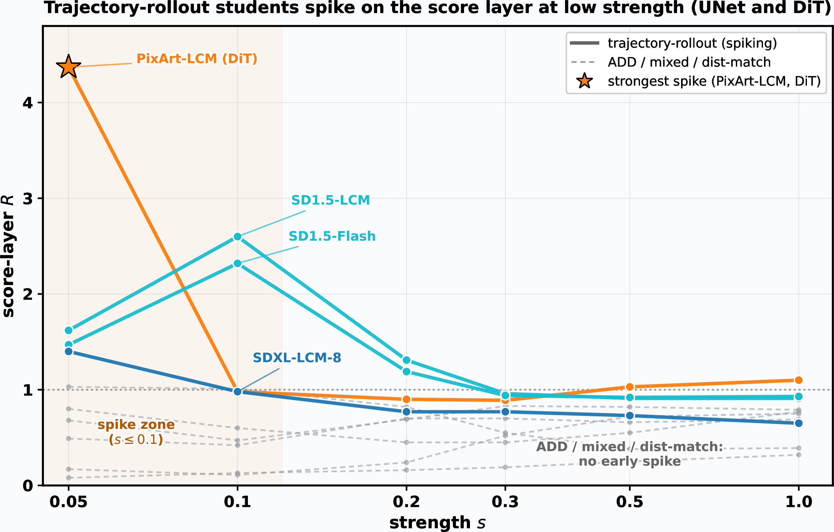
The score layer carries a second, shape-based signal. Some students exhibit a localized early-strength spike: the score ratio rises above \(1\) at low strength (with a CI strictly above \(1\)) and then falls, so that the low-\(s\) peak (\(s\!\leq\!0.1\)) is CI-separated above the \(s\!=\!0.5\) value (Figure 3, Table 6). Under this criterion the spike appears only on students whose loss trains on student or generated trajectory segments (our operational trajectory-rollout label, which does not imply the absence of auxiliary adversarial terms): LCM on both UNet backbones (SDXL-LCM at \(8\) steps), Flash (backward-simulation) on SD1.5, and most strongly PixArt-LCM on a pure DiT backbone (peak \(4.37\) [\(4.28\), \(4.45\)] at \(s\!=\!0.05\), the largest distilled spike in the sweep). No tested ADD, mixed, or distribution-matching representative satisfies the CI-separated spike criterion: their score ratios have no CI-separated low-\(s\) peak above \(1\). Within the full released sweep the spike is thus exclusive to trajectory-rollout among the tested paradigms, though not universal within it (SDXL-LCM at \(4\) steps does not reach the threshold, so magnitude is step- and backbone-dependent). The most tempting counterexample, FLUX-schnell (ADD), has low-\(s\) score \(1.03\) [\(0.98\), \(1.08\)] — a peak whose CI straddles \(1\) — so it does not meet the criterion; the DiT/MMDiT ADD controls (SD3.5-Turbo, FLUX-schnell) show no spike, so on DiT the spike still separates trajectory-rollout from ADD. The spike is thus associated with trajectory-rollout objectives and observed on both UNet and DiT, while its appearance and magnitude shift with step count and backbone.
| Backbone \(\times\) paradigm | Arch. | low-\(s\) peak [CI] | \(s\!=\!0.50\) [CI] | spike? |
|---|---|---|---|---|
| PixArt \(\times\) LCM-4 | DiT | 4.37 [4.28, 4.45] | 1.03 [1.03, 1.03] | ✔✔ |
| SD1.5 \(\times\) LCM-4 | UNet | 2.60 [2.59, 2.61] | 0.91 [0.91, 0.92] | ✔ |
| SD1.5 \(\times\) Flash-4 | UNet | 2.32 [2.30, 2.34] | 0.92 [0.92, 0.92] | ✔ |
| SDXL \(\times\) LCM-8 | UNet | 1.40 [1.35, 1.45] | 0.73 [0.73, 0.73] | ✔ |
| FLUX \(\times\) schnell-4 (ADD) | DiT | 1.03 [0.98, 1.08] | 0.38 [0.36, 0.39] | \(\times\)\(\ast\) |
| SDXL \(\times\) LCM-4 | UNet | 0.76 [0.74, 0.78] | 0.68 [0.67, 0.68] | \(\times\) |
| SDXL \(\times\) Lightning-4 | UNet | 0.14 | 0.69 | \(\times\) |
| SD1.5 \(\times\) Hyper-4 | UNet | 0.46 | 0.77 | \(\times\) |
| SDXL \(\times\) Hyper-8 | UNet | 0.17 | 0.72 | \(\times\) |
| SDXL \(\times\) DMD2-1 | UNet | 0.58 | 0.62 | \(\times\) |
| SDXL \(\times\) Turbo-4 (ADD) | UNet | 0.49 | 0.66 | \(\times\) |
| SD1.5 \(\times\) SD-Turbo-4 (ADD) | UNet | 0.31 | 0.60 | \(\times\) |
| SD3.5 \(\times\) Turbo-4 (ADD) | MMDiT | 0.80 | 0.55 | \(\times\) |
6pt
4.5.0.1 Latent contamination caveat.
PixArt-LCM also shows a latent excursion at the two lowest strengths (\(9.53\) at \(s\!=\!0.05\), \(1.76\) at \(s\!=\!0.1\)) co-located with its score spike. This is not the band-shaped RF latent signature of Section 4.3 (which is sustained across \(s\!\in\![0.05, 0.3]\) on SD3.5/FLUX); it is the same trajectory-rollout sensitivity surfacing in both layers at low strength, and it collapses below \(1\) by \(s\!=\!0.2\). Because the RF signature is read as a sustained band rather than a single low-\(s\) crossing, this isolated two-cell excursion does not classify PixArt-LCM as rectified-flow (Table 4).
4.6 Distillation Amplifies Prompt Collapse Strongly on SD1.5, Weakly Elsewhere↩︎
A final observation uses the architecture-matched teacher/student pairs. Comparing the prompt-layer peak ratio of each student against its own teacher, distillation amplifies prompt-mean collapse strongly on SD1.5, only weakly and inconsistently on SDXL, and near-neutrally on the DiT/MMDiT pairs (Table 7). We report this as an observation rather than a law: the comparison is peak-versus-peak (the peaks sit at different strengths on teacher and student), SDXL’s students straddle their teacher (the amplification is carried by SD1.5), and the non-UNet families contribute a single student each.
| Family | Arch. | best student peak / teacher peak |
|---|---|---|
| SD1.5 | UNet | 13.32 / 5.20 = 2.56\(\times\) |
| SDXL | UNet | 7.98 / 6.88 = 1.16\(\times\)\(\S\) |
| SD3.5 | MMDiT | 21.05 / 17.91 = 1.18\(\times\) |
| PixArt-\(\alpha\) | DiT | 7.30 / 7.93 = 0.92\(\times\) |
| FLUX | DiT | 23.66 / 26.25 = 0.90\(\times\) |
6pt
5 Discussion↩︎
5.1 What the probe establishes, and what it does not↩︎
The three layers read three empirically separable factors (Section 4.2), and the strongest of the three readings is the latent layer. The rectified-flow detector (Section 4.3) rests on a clean separation (two RF backbones pass, three \(\epsilon\)-prediction backbones do not), a control that removes the obvious confound (PixArt-\(\alpha\) holds T5 conditioning fixed but is \(\epsilon\)-prediction and does not pass), and four RF cases spanning teacher/student and MMDiT/DiT. We state this as a property of the prediction type that survives the distillation runs we tested — both pure-adversarial (ADD) — and not as a claim about every possible RF distillation: we did not test a non-ADD RF student, so “survives ADD” is the precise statement. We do not claim that this criterion is a universal rectified-flow detector outside the tested public checkpoints; it is the factor that cleanly separates this sweep.
The score-layer findings are deliberately scoped narrower. Finding 2 is a binary ADD-vs-non-ADD detector, not a five-paradigm ranking: the four non-ADD paradigms are not pairwise separable at \(s\!=\!0.5\) and step count confounds any finer ordering (Section 4.4). Finding 3 is associated with trajectory-rollout objectives and observed on both UNet and DiT, but its appearance and magnitude depend on step count and backbone (SDXL-LCM spikes at \(8\) steps but not \(4\)), and each non-UNet paradigm is represented by a single student. The amplification observation (Section 4.6) is a peak-versus-peak comparison on single non-UNet students and is reported as an observation, not a law.
5.2 Limitations↩︎
The probe is white-box: it requires the model weights and forward code to install the hooks, so it does not perform image-only detection. The non-UNet coverage is three students (ADD on MMDiT and DiT; trajectory on DiT); we have no non-ADD RF student and no distribution-matching or mixed student off UNet, so the latent fingerprint is shown to survive ADD only, and the score-layer paradigm structure is densest on UNet. Most students are measured at a single seed (cross-seed robustness was established on the SDXL zoo in earlier work). One reading is contaminated at low strength: trajectory-rollout students show a spurious latent excursion at the two lowest strengths, which is why the RF fingerprint is read as a sustained low-to-mid band rather than a single low-\(s\) crossing (Section 4.5).
5.3 Toward a downstream use↩︎
This paper stops at the instrument and its readings. Two downstream uses are natural but deliberately left to future work. First, the score layer reads a property — the distillation objective — that is not recoverable from the weights or configuration, so auditing an undisclosed training recipe from a released checkpoint is a non-circular application; by contrast, detecting the architecture via the latent layer is circular, since the prediction type is already declared in the model configuration, and we do not claim it as an application. Second, the per-layer readings could serve as a during-training signal to guide distillation. Both require an evaluation we do not undertake here, and we make no downstream claim in this version.
6 Conclusion↩︎
We presented a decomposable, layer-/mode-resolved probe for diffusion text-to-image models, and applied it under a single matched estimator to a \(23\)-model sweep spanning five backbone families, three architecture classes, and five distillation paradigms. The probe’s three injection layers turn out to read three empirically separable factors — a universal prompt-conditioning response on the prompt layer, the prediction type on the latent layer, and the distillation objective on the score layer. Within this sweep the latent layer in particular is a near-binary detector of rectified-flow backbones that survives ADD distillation, under the sustained-band criterion, with the obvious wide-T5-conditioning explanation ruled out by a matched \(\epsilon\)-prediction control and four RF cases across two architecture families and teacher/student roles; two further cross-family findings — a binary ADD-vs-non-ADD score detector and a trajectory-rollout early-strength spike present on both UNet and DiT — complete the picture. We release all per-cell CI-citable tables and the matched estimator. Turning these readings into a downstream use — auditing an undisclosed distillation recipe, or guiding distillation during training — is the natural next step.
7 Bures Estimator: Plug-in Bias and Bootstrap-Median Fix↩︎
This appendix records the estimator decision behind every \(R_\text{lo}\) number reported in the main text. The squared-Wasserstein-2 ratio \(R_\text{sel}\) defined in eq. 1 is evaluated on the true Bures \(W_2^2\) functional applied to Inception-v3 pool3 statistics, computed via a low-rank Gram form, on every one of the 23 models in the sweep. At our operating cell sizes (\(n\!\approx\!1500\)–\(2000\), \(d\!=\!2048\)) the plug-in estimator \(W_2^2(\widehat{\mu},\widehat{\Sigma})\) inherits a non-linear functional bias: because the Bures functional is non-linear in the covariance, its plug-in does not coincide with the bootstrap distribution of the same functional, so the plug-in point estimate does not in general fall inside the bootstrap percentile interval; we therefore adopt the bootstrap-median percentile estimator below as the single-distribution headline.
7.0.0.1 Bootstrap-median estimator.
We replace the plug-in with a bootstrap-median percentile estimator: \(n_\text{resample}\) resamples of the prompt set, the median of the resampled ratios is reported as \(R_\text{point}\), and the \(5/95\)th percentiles as \([R_\text{lo}, R_\text{hi}]\), i.e.a \(90\%\) percentile interval. This is the headline statistic on every model in the main text. The plug-in value is retained in our release for audit purposes; it is never the bar a claim is checked against. All cross-backbone comparison cells use the base-fixed bootstrap-median estimator with \(n_\text{resample}\!=\!200\) and a fixed seed, applied identically to every model in the sweep so that all ratios are estimator-matched.
7.0.0.2 Matched across backbones.
The single methodological requirement for the cross-backbone claims is that the same estimator is applied to every model. We confirm that SDXL, SD1.5, SD3.5, PixArt-\(\alpha\), and FLUX teachers and all 18 students are computed under base-fixed bootstrap-median true Bures \(W_2^2\). For the record, a fast diagonal-covariance proxy was used for early exploratory sweeps but for no cell in this paper: it drops the cross-dimension covariance terms and biases the selectivity ratio relative to the true Bures functional, with a direction that depends on the cell (the sign is not uniform across layers/strengths). Rather than rely on any fixed-sign argument, every cross-backbone cell is recomputed with the true functional so that all \(23\) models are estimator-comparable.
8 Architecture / Paradigm Master Mapping↩︎
Table 8 records the \(2\!\times\!2\) disambiguation that attributes the latent fingerprint to the prediction type rather than the text-conditioning width: PixArt-\(\alpha\) is the \((\epsilon\text{-pred}, \text{T5})\) cell that falsifies the wide-conditioning hypothesis.
| \(\epsilon\)-prediction | rectified-flow | |
|---|---|---|
| T5 (+ CLIP) | PixArt-\(\alpha\): no band (peak \(1.13\)) (\(\times\)) | SD3.5: band, peak \(13.01\) (✔); FLUX: band, peak \(7.31\) (\(28\)-step) (✔) |
| CLIP only | SDXL, SD1.5: no band (\(\times\)) | (none in sweep) |
6pt
9 Per-Backbone Full Sweep Tables↩︎
All cells are \(R_\text{point}\) with \([R_\text{lo}, R_\text{hi}]\) in brackets, base-fixed bootstrap-median true Bures \(W_2^2\), \(n_\text{resample}\!=\!200\), full \(3\)-layer \(\times\) \(6\)-strength grid. Latent and score columns give \(R_\text{point}\) (CIs in the released JSON). We group by family; teachers first.
9.0.0.1 Non-UNet teachers: RF backbones (SD3.5, FLUX) and the \(\epsilon\)-prediction control (PixArt-\(\alpha\)).
Table 9 gives the non-UNet teachers: SD3.5 and FLUX as the rectified-flow cases, and PixArt-\(\alpha\) as the matched T5 \(\epsilon\)-prediction control. The latent column is the load-bearing one for Section 4.3.
| Teacher | layer | \(s\!=\!0.05\) | \(s\!=\!0.1\) | \(s\!=\!0.2\) | \(s\!=\!0.3\) | \(s\!=\!0.5\) | \(s\!=\!1.0\) |
|---|---|---|---|---|---|---|---|
| SD3.5 (28, RF) | prompt | 1.36 | 1.42 | 1.59 | 3.27 | 17.91 | 1.93 |
| latent | 13.01 | 12.37 | 8.22 | 3.96 | 1.30 | 1.08 | |
| score | 0.66 | 0.45 | 0.39 | 0.42 | 0.47 | 0.77 | |
| PixArt-\(\alpha\) (20, \(\epsilon\)) | prompt | 1.76 | 2.41 | 5.64 | 7.93 | 7.85 | 2.18 |
| latent | 0.61 | 1.13 | 0.80 | 0.90 | 1.00 | 1.05 | |
| score | 0.64 | 0.91 | 0.89 | 0.98 | 1.02 | 0.97 | |
| FLUX.1-dev (28, RF) | prompt | 1.81 | 7.17 | 24.14 | 25.44 | 19.38 | 1.45 |
| latent | 2.17 | 7.31 | 4.23 | 1.18 | 0.93 | 0.99 | |
| score | 0.98 | 0.93 | 1.00 | 0.96 | 0.73 | 0.61 | |
| FLUX.1-dev (50, RF) | prompt | 1.84 | 7.12 | 24.95 | 26.25 | 20.92 | 1.49 |
| latent | 1.68 | 8.21 | 4.46 | 1.12 | 0.93 | 0.99 | |
| score | 0.99 | 0.93 | 0.96 | 0.93 | 0.74 | 0.60 |
4pt
9.0.0.2 Non-UNet students (SD3.5-Turbo, PixArt-LCM, FLUX-schnell).
Table 10 gives the three non-UNet distilled students. The two ADD students (SD3.5-Turbo, FLUX-schnell) retain the latent fingerprint band; PixArt-LCM shows the low-strength latent excursion (\(9.53\) at \(s\!=\!0.05\), \(1.76\) at \(s\!=\!0.1\)) flagged in Section 4.5 and the strongest score early-spike in the sweep.
| Student | layer | \(s\!=\!0.05\) | \(s\!=\!0.1\) | \(s\!=\!0.2\) | \(s\!=\!0.3\) | \(s\!=\!0.5\) | \(s\!=\!1.0\) |
|---|---|---|---|---|---|---|---|
| SD3.5-Turbo-4 (ADD) | prompt | 1.45 | 1.57 | 1.84 | 2.21 | 21.05 | 1.99 |
| latent | 8.88 | 15.27 | 7.23 | 3.21 | 1.32 | 1.11 | |
| score | 0.80 | 0.60 | 0.45 | 0.45 | 0.55 | 0.77 | |
| PixArt-LCM-4 (traj.) | prompt | 2.04 | 2.36 | 4.38 | 7.30 | 5.15 | 2.00 |
| latent | 9.53 | 1.76 | 0.74 | 0.91 | 1.01 | 1.05 | |
| score | 4.37 | 0.98 | 0.90 | 0.89 | 1.03 | 1.10 | |
| FLUX-schnell-4 (ADD) | prompt | 1.74 | 6.56 | 23.66 | 21.05 | 16.15 | 1.98 |
| latent | 2.03 | 3.61 | 5.53 | 2.73 | 0.93 | 0.97 | |
| score | 1.03 | 1.01 | 0.82 | 0.55 | 0.38 | 0.39 |
4pt
9.0.0.3 UNet teachers and students (SDXL, SD1.5).
Tables 11 and 12 give the full per-cell \(R_\text{point}\) grid for the two UNet families. Every latent row stays below \(1\) at low strength (no rectified-flow fingerprint, Section 4.3); the score column at \(s\!=\!0.5\) carries the ADD-detector ordering (Section 4.4), and the SDXL-LCM-8 / SD1.5-LCM / SD1.5-Flash score rows carry the low-strength spike (Section 4.5).
| Model (SDXL) | layer | \(s\!=\!0.05\) | \(s\!=\!0.1\) | \(s\!=\!0.2\) | \(s\!=\!0.3\) | \(s\!=\!0.5\) | \(s\!=\!1.0\) |
|---|---|---|---|---|---|---|---|
| SDXL teacher (50) | prompt | 1.37 | 1.33 | 1.48 | 2.08 | 4.58 | 6.88 |
| latent | 0.36 | 0.17 | 0.12 | 0.16 | 0.27 | 0.61 | |
| score | 0.20 | 0.14 | 0.25 | 0.52 | 0.80 | 0.80 | |
| SDXL DMD2-1 | prompt | 1.94 | 2.56 | 4.04 | 6.08 | 6.65 | 2.51 |
| latent | 0.22 | 0.57 | 0.73 | 0.68 | 0.66 | 0.69 | |
| score | 0.14 | 0.58 | 0.77 | 0.68 | 0.62 | 0.65 | |
| SDXL DMD2-4 | prompt | 1.12 | 1.13 | 1.31 | 1.71 | 2.74 | 3.03 |
| latent | 0.40 | 0.20 | 0.23 | 0.47 | 0.76 | 0.78 | |
| score | 0.68 | 0.47 | 0.69 | 0.83 | 0.82 | 0.79 | |
| SDXL Hyper-1 | prompt | 1.49 | 1.46 | 1.63 | 2.02 | 3.84 | 1.45 |
| latent | 0.14 | 0.20 | 0.36 | 0.51 | 0.64 | 0.74 | |
| score | 0.12 | 0.19 | 0.40 | 0.37 | 0.35 | 0.32 | |
| SDXL Hyper-4 | prompt | 1.32 | 1.26 | 1.36 | 1.71 | 2.99 | 1.65 |
| latent | 0.21 | 0.15 | 0.22 | 0.38 | 0.64 | 0.75 | |
| score | 0.11 | 0.11 | 0.36 | 0.63 | 0.69 | 0.73 | |
| SDXL Hyper-8 | prompt | 1.29 | 1.23 | 1.30 | 1.65 | 3.33 | 1.97 |
| latent | 0.35 | 0.17 | 0.16 | 0.26 | 0.43 | 0.71 | |
| score | 0.17 | 0.11 | 0.24 | 0.52 | 0.72 | 0.75 | |
| SDXL LCM-4 | prompt | 1.51 | 1.51 | 2.03 | 3.48 | 6.01 | 3.85 |
| latent | 0.22 | 0.21 | 0.34 | 0.54 | 0.63 | 0.68 | |
| score | 0.76 | 0.44 | 0.72 | 0.67 | 0.68 | 0.68 | |
| SDXL LCM-8 | prompt | 1.49 | 1.57 | 3.00 | 5.51 | 7.98 | 4.45 |
| latent | 0.19 | 0.14 | 0.22 | 0.29 | 0.37 | 0.58 | |
| score | 1.40 | 0.98 | 0.77 | 0.77 | 0.73 | 0.65 | |
| SDXL Lightning-4 | prompt | 1.38 | 1.32 | 1.35 | 1.56 | 2.91 | 1.82 |
| latent | 0.21 | 0.16 | 0.21 | 0.31 | 0.53 | 0.76 | |
| score | 0.14 | 0.13 | 0.35 | 0.68 | 0.69 | 0.73 | |
| SDXL Turbo-1 | prompt | 1.61 | 1.69 | 1.97 | 2.29 | 2.81 | 1.31 |
| latent | 0.13 | 0.25 | 0.46 | 0.55 | 0.57 | 0.77 | |
| score | 0.13 | 0.25 | 0.50 | 0.50 | 0.49 | 0.46 | |
| SDXL Turbo-4 | prompt | 1.41 | 1.49 | 1.70 | 1.99 | 2.74 | 1.21 |
| latent | 0.79 | 0.41 | 0.35 | 0.48 | 0.55 | 0.71 | |
| score | 0.49 | 0.42 | 0.70 | 0.70 | 0.66 | 0.69 |
4pt
| Model (SD1.5) | layer | \(s\!=\!0.05\) | \(s\!=\!0.1\) | \(s\!=\!0.2\) | \(s\!=\!0.3\) | \(s\!=\!0.5\) | \(s\!=\!1.0\) |
|---|---|---|---|---|---|---|---|
| SD1.5 teacher (50) | prompt | 1.75 | 2.65 | 5.20 | 5.16 | 3.37 | 1.20 |
| latent | 0.65 | 0.41 | 0.31 | 0.24 | 0.23 | 0.52 | |
| score | 0.39 | 0.33 | 0.47 | 0.61 | 0.80 | 0.91 | |
| SD1.5 LCM-4 | prompt | 5.34 | 7.38 | 13.32 | 12.80 | 7.18 | 1.38 |
| latent | 0.99 | 0.34 | 0.45 | 0.45 | 0.61 | 0.74 | |
| score | 1.62 | 2.60 | 1.31 | 0.96 | 0.91 | 0.91 | |
| SD1.5 Flash-4 | prompt | 2.02 | 4.38 | 7.79 | 6.48 | 2.42 | 1.50 |
| latent | 1.05 | 0.67 | 0.20 | 0.19 | 0.36 | 0.55 | |
| score | 1.47 | 2.32 | 1.19 | 0.94 | 0.92 | 0.93 | |
| SD1.5 Hyper-4 | prompt | 2.25 | 4.24 | 7.77 | 5.89 | 2.50 | 1.49 |
| latent | 0.83 | 0.45 | 0.24 | 0.32 | 0.57 | 0.87 | |
| score | 0.46 | 0.29 | 0.64 | 0.78 | 0.77 | 0.86 | |
| SD1.5 SD-Turbo-1 | prompt | 1.55 | 1.41 | 1.66 | 2.06 | 4.03 | 1.51 |
| latent | 0.10 | 0.13 | 0.33 | 0.49 | 0.69 | 0.73 | |
| score | 0.08 | 0.13 | 0.16 | 0.19 | 0.25 | 0.32 | |
| SD1.5 SD-Turbo-4 | prompt | 1.27 | 1.35 | 1.71 | 2.40 | 3.29 | 1.47 |
| latent | 0.17 | 0.20 | 0.36 | 0.31 | 0.34 | 0.36 | |
| score | 0.25 | 0.31 | 0.47 | 0.55 | 0.60 | 0.63 |
4pt
References↩︎
Independent Researcher.
patrickmupersonal@outlook.com↩︎FLUX.1 uses a hybrid transformer with both double-stream (MMDiT-style) and single-stream blocks; we write “DiT” as shorthand and treat SD3.5 and FLUX as two rectified-flow backbone families rather than as fully independent architectures.↩︎
A width below \(0.005\) collapses to a point under two-decimal rounding; the full-precision intervals are in the released per-cell tables.↩︎