Graph Neural Networks for the Graphical Bootstrap
July 03, 2026
Abstract
We study a graph classification problem involving over 20 million graphs, arising from high-order perturbative computations of correlators in planar \(\mathcal{N}=4\) super-Yang–Mills, a model closely related to the theory of the strong nuclear force. We benchmark graph neural networks, including graph transformers, achieving robust generalization to larger graphs with up to \(99.996\%\) ROC AUC. Then, we analyze how the models can be used to gain a computational speedup compared to the traditional graphical bootstrap algorithm, through shrinking the redundant data by up to \(85.5\%\) at the level of denominator graphs. Finally, we study the embeddings of the models to investigate their interpretability.
1 Introduction↩︎
With the upcoming high-luminosity upgrade of the LHC, particle-physics data are expected to reach unprecedented precision. To match this and further test our understanding of the underlying physics, comparably precise higher-order perturbative calculations are required. The object of interest is typically the scattering amplitude, whose perturbative expansion translates into diagrams with increasing number of vertices, while the number of such diagrams grows factorially with each perturbative order. This increase in complexity requires identifying new structures and simplifications. An ideal setting to develop and test such new ideas is \(\mathcal{N}=4\) super Yang-Mills theory (SYM) [1].
In particular, we focus on 4-point correlator integrands (a simple limit of which yields amplitude integrands) in planar \(\mathcal{N}=4\) SYM. These have been computed to higher and higher orders in perturbation theory over many years [2]–[7] culminating in the recent remarkable 12-th order result [8]. The four point integrand at \(\ell\)-th perturbative order, is a permutation invariant rational function of \(n=4+{\ell}\) spacetime points \(x_{1},\ldots,x_{n}\), allowing for an ansatz expansion in purely combinatorial objects, \[\label{eq:ansatz} f^{(n)}(x_1,\ldots,x_{n}) = \sum_{a,b} c^{(n)}_{a,b} \textcolor{blue}{f^{(n)}_{a,b}}(x_1,\ldots,x_{n}) \,.\tag{1}\] Here the \(c^{(n)}_{a,b}\) are numerical coefficients and \(\textcolor{blue}{f^{(n)}_{a,b}}\) are permutation invariant functions of \(x_i\). Strong physical requirements allow us to associate these functions with graphs, called \(f\)-graphs [3], [4], which have \(n\) nodes and two types of edges, numerator edges, \(N(f_{a,b}^{(n)})\), and denominator edges, \(D(f_{a,b}^{(n)})\). The denominator edges alone must form a planar graph, and the net (denominator minus numerator) valency at each vertex must be four. The precise relation is \[\label{fgraphs} \textcolor{blue}{f^{(n)}_{a,b}}(x_1,\ldots,x_{n}) = \sum_{\sigma \in S_{n}} \frac{1}{|\text{Aut}(f^{(n)}_{a,b})|} \frac{\prod_{(ij)\in N(f^{(n)}_{a,b})} x_{ij}^2}{\prod_{(ij) \in D(f^{(n)}_{a,b})} x_{ij}^2}\,.\tag{2}\] Here \(x_i\) only appears through distance pairs \(x_{ij}^2:=(x_{i}-x_{j})^2\), \(|\text{Aut}(f_{a,b}^{(n)})|\) is the graph symmetry factor and \(S_{n}\) represents the \(n\)-point permutation group. The full set of relevant f-graphs is generated by first drawing all physically allowed denominator graphs and then dressing them with numerator edges in all possible ways. The label \(a\) runs over the various denominator graphs (black lines) while \(b\), whose relevance only begins at \(n=10\), the different dressings with numerator edges (blue, dashed lines). For example at 8 points in figure 1 there are only 3 possible \(f\)-graphs, the first two admit a single numerator decoration while the third one none. Here all coefficients have values \(\pm1\), whereas at higher \(n\), zero coefficients, higher integers and fractional coefficients appear. The statistics of \(f\)-graphs and denominator graphs (\(d\)-graphs) are shown in table 1.
| # nodes | \(\leq 9\) | 10 | 11 | 12 | 13 | 14 | 15 | 16 |
|---|---|---|---|---|---|---|---|---|
| # \(f\)-graphs | 13 | 36 | 220 | 2,707 | 42,979 | 898,353 | 22,024,902 | 619,981,403 |
| # \(d\)-graphs | 13 | 31 | 164 | 1,430 | 13,936 | 152,009 | 1,697,302 | 19,212,867 |
| % Vanishing \(c_{a,b}\) | 0 | 28 | 42 | 61 | 76 | 85 | 91 | 94 |
| % Vanishing \(d_{a}\) | 0 | 27 | 35 | 49 | 59 | 66 | 71 | 75 |

The computation of each perturbative term progresses by constructing an ansatz as in 1 using all allowed f-graphs. Physical constraints translate into graphical rules [6] (the graphical bootstrap) such as the “rung rule” (Figure [fig:rung95rule]), which replaces a squared face with a pyramid dressed with numerator edges on the diagonals, or the more powerful “cusp rule” [7], [8], providing linear equations among the various \(c_{a,b}^{(n)}\). The rung rule is very simple but leaves many coefficients undetermined (14% at \(n=16\)), whereas the cusp rule is more complete and may give a unique solution for all coefficients [7]. However, as shown in Table 1, the number of \(f\)-graphs grows factorially; at \(n=16\), the cusp rule yields a system of approximately \(10^{10}\) sparse equations that required 3 days on an HPC cluster to be solved [8]. At \(n > 16\), the construction and solution of such systems become computationally prohibitive.
One would like to use machine learning to predict the graph coefficients directly. However, as with all exact analytic results, ultimately 100% accuracy is sought. Instead therefore, we propose a more modest goal which will have immediate practical use without needing such high accuracy. Although the number of graphs grows to a monstrous scale, exceeding 600 million at \(n = 16\), the ansatz becomes increasingly redundant, with \(94\%\) of \(f\)-graphs not contributing (table 1). Rather than predicting the coefficients themselves, we use machine learning to identify graphs that can be discarded \((c_{a,b}^{(n)}=0)\). We simplify further, by considering families of graphs with the same underlying denominator together (\(d\)-graphs) and so predict the binary coefficient: \[\label{eq:dengraph} d^{(n)}_a = \begin{cases} 0 & \text{if } c^{(n)}_{a,b}=0 \;\forall b \\ 1 & \text{otherwise} \end{cases}\tag{3}\] which simply states that if all numerator dressings of a denominator graph vanish, it has label 0, otherwise 1. This reduces the problem to a binary classification task on simple unlabelled planar graphs. Since the system is solvable only when all graphs with coefficients equal to 1 are present, we require \(100\%\) recall on positives. The reduction of the redundant fraction of the ansatz is then quantified by the True Negative Rate (TNR), which measures the fraction of correctly identified negative-class graphs.
1.0.0.1 Related work
The use of machine learning to obtain exact or symbolic results in theoretical high-energy physics has recently attracted growing attention, see for example [9]. This work employs Transformers to predict exact coefficient data in planar \(\mathcal{N}=4\) SYM correlators. Related directions include symbolic amplitude computation using machine learning [10] and the simplification of polylogarithmic expressions [11].
2 Models, features and methodology↩︎
We benchmark three architectures: Graph Isomorphism Network (GIN) [12], Graph Attention Network (GAT) [13], and Graphormer (GT) [14]. This enables a direct comparison between message passing, attention-based message passing, and transformer-style global attention within a unified setup.
All models share the same node inputs that combine three feature families: centrality scores (degree, clustering, betweenness, closeness, PageRank) [15], top-3 Laplacian eigenvectors as positional encodings [16], and graphlet orbit counts up to \(k=4\) [17]. Since the coefficients are constrained by physical properties of the correlator that depend on graph substructures, we select features sensitive to local structural patterns.
GIN and GAT share a backbone of \(L\) layers with batch normalization, Jumping Knowledge [18], and an MLP head; GIN uses sum pooling, GAT attention pooling with residuals. The GT uses a pre-LayerNorm Transformer [19] with global self-attention and adjacency/shortest-path biases.
Each experiment involves training on graphs with up to \(n\) nodes and predicting coefficients for graphs with \(n+1\) nodes, we refer to them as \(n\!\to\! n+1\). Graphs with \(n \leq 9\) have distinct statistical properties (no vanishing coefficients) so we exclude these. This binary classification task faces an increasing distribution shift, as class imbalance grows with \(n\) (table 1). To ensure cross-size generalization, hyperparameters were selected by training on \(10\le N\le n-1\) node graphs and validating on \(n\)-node graphs (i.e., a graph-size based split rather than a random partition). Then we ran a 300-point random grid search (learning rate \(5\cdot10^{-5}-5\cdot10^{-3}\), weight decay \(5\cdot10^{-7}-10^{-3}\), dropout 0.2–0.5, 2–5 layers, 4–128 hidden channels, batch size 4–256; GT heads 8–32) for 10 epochs. Finally, models with the hyperparameters of the six best runs (top-3 by validation loss and top-3 by validation ROC AUC) are trained for 100 epochs on the full \(10,\ldots,n\) data and we adopt the average of their raw outputs as per model predictions. Optimization uses Adam, binary cross-entropy-with-logits, and OneCycle scheduling. Training runs on 1–4 GPUs (A100/V100 class), with the heaviest jobs taking 8–12 hours.
3 Experiments, results and interpretability↩︎
3.0.0.1 Ranking and class separability
Models are trained up to \(12\leq n \leq 15\) node graphs and always tested on \(n+1\) ones, matching the physics setting where \(d_{a}^{(n+1)}\) are inferred from \(d_{a}^{(n)}\). We are eventually interested in the ansatz reduction task (requiring 100% recall), but it is initially interesting to consider the ranking of predicted probabilities among the two classes and analyse the choice of a threshold in the next paragraph.
To this end, Table 2 reports ROC AUC of the three architectures on different training setups. We observe a strong performance across all experiments , which improves, despite stronger class imbalance, at higher \(n\). GT is consistently the best, reaching an impressive \(99.996\%\), while GIN becomes competitive only when training includes at least \(n=13\) data. The results strongly indicate that, indeed, the graphs constitute a learnable dataset, since despite the distribution shift between training and testing there is a strong threshold independent class separation.
| 12 \(\!\to\!\) 13 | 13 \(\!\to\!\) 14 | 14 \(\!\to\!\) 15 | 15 \(\!\to\!\) 16 | |
|---|---|---|---|---|
| GIN | 88.608 | 95.647 | 98.534 | 98.600 |
| GAT | 89.597 | 95.679 | 97.871 | 98.137 |
| GT | 97.921 | 99.459 | 99.959 | 99.996 |
To interpret these results from a physics perspective, we ask how well the models capture the simplest among the graphical rules, the rung rule, which under the denominator-graph labelling in 3 , only relates graphs of positive class (\(d_a=1\)). To quantify the effect we compute the probability of superiority [20] between rung-rule-generated data and its complement in the positive class across all experiments. GIN and GAT show weak-to-moderate separation (\(50\)–\(55\%\) and \(48\)–\(69\%\), respectively), whereas GT shows a stronger effect, increasing from \(61\%\) to \(86\%\) as training size grows. This indicates that GT captures rung-rule relevant substructures more effectively which is justified by the access that the Transformer architecture provides to complicated graph substructures.
3.0.0.2 Ansatz reduction
Next, the ansatz reduction task is addressed with special focus on its operational constraint (100% Recall) which is threshold-sensitive. We ask: is there a threshold satisfying the constraint that can be estimated robustly while also removing a substantial fraction of the ansatz? We define \(\mathbf{t_{\mathrm{train}}}\) (\(\mathbf{t_{\mathrm{test}}}\)) as the minimum predicted probability over true positives in the training (test) dataset for each model. Thus, \(\mathbf{t_{\mathrm{test}}}\) is the optimal threshold: the smallest value that guarantees zero false negatives (FN). We observe that no predictable mapping from \(\mathbf{t_{\mathrm{train}}}\) to \(\mathbf{t_{\mathrm{test}}}\) exists across architectures and experiments. GAT is the most stable: \(\mathbf{t_{\mathrm{train}}}/10\) guarantees zero false negatives across all experiments while still hitting a high TNR, reaching \(43.5, 50.4\) and \(50\%\) for \(n+1=14,15,16\) respectively. For GIN and GT, in contrast, the optimal threshold can lie several orders of magnitude below \(\mathbf{t_{\mathrm{train}}}\) (Table 3).
| \(\mathbf{t_{\mathrm{train}}}\) | \(\mathbf{t_{\mathrm{test}}}\) | FN @ \(\mathbf{t_{\mathrm{train}}}\) | FN @\(\mathbf{t_{\mathrm{train}}}/10\) | TNR @\(\mathbf{t_{\mathrm{train}}}/10\) | TNR @\(\mathbf{t_{\mathrm{test}}}\) | |
|---|---|---|---|---|---|---|
| GIN | 0.026 | \(1.14\cdot10^{-5}\) | 252 | 29 | 47.5 % | 4% |
| GAT | 0.27 | 0.10 | 82 | 0 | 50% | 61.0% |
| GT | 0.47 | \(5\cdot10^{-9}\) | 18193 | 1053 | 99.3% | 85.5% |
Threshold selection could be coupled to the linear solve: start from a candidate threshold, and decrease it if the reduced ansatz yields no solution. An analysis of the efficiency gain of such a pipeline is left for the future. Here we quantify pruning: with optimal threshold GAT and GT remove up to \(61\%\) and \(85.5\%\) of the redundant \(d\)-graph sector respectively (millions of graphs), with GT improving from \(42.6\%\) at \(n+1=13\) to \(85.5\%\) at \(n+1=16\).
3.0.0.3 Interpretability
We extract graph embeddings and train linear probes to predict pre-computed graph-level features [21], testing whether global structure is encoded in the representations. We consider standard cycle counts \(C_3,C_4,C_5\) and induced 4-node graphlets \(\begin{tikzpicture}[ baseline={([yshift=.3ex]current bounding box.south)}, scale=0.2, every node/.style={circle,fill=black,inner sep=0.9pt}, edge/.style={black,thin,line cap=round,line join=round} ] \coordinate (TL) at (0,1); \coordinate (TR) at (1.15,1); \coordinate (BL) at (0,0); \coordinate (BR) at (1.15,0); \draw[edge] (TL)--(TR); \draw[edge] (TL)--(BL); \draw[edge] (BL)--(BR); \node at (TL) {}; \node at (TR) {}; \node at (BL) {}; \node at (BR) {}; \end{tikzpicture},\begin{tikzpicture}[ baseline={([yshift=.3ex]current bounding box.south)}, scale=0.2, every node/.style={circle,fill=black,inner sep=0.9pt}, edge/.style={black,thin,line cap=round,line join=round} ] \coordinate (TL) at (0,1); \coordinate (TR) at (1.15,1); \coordinate (BL) at (0,0); \coordinate (BR) at (1.15,0); \draw[edge] (TL)--(TR)--(BR)--(BL)--cycle; \node at (TL) {}; \node at (TR) {}; \node at (BL) {}; \node at (BR) {}; \end{tikzpicture},\begin{tikzpicture}[ baseline={([yshift=.3ex]current bounding box.south)}, scale=0.2, every node/.style={circle,fill=black,inner sep=0.9pt}, edge/.style={black,thin,line cap=round,line join=round} ] \coordinate (TL) at (0,1); \coordinate (TR) at (1.15,1); \coordinate (BL) at (0,0); \coordinate (BR) at (1.15,0); \draw[edge] (TL)--(TR); \draw[edge] (TL)--(BL); \draw[edge] (BL)--(BR); \draw[edge] (BL)--(TR); \node at (TL) {}; \node at (TR) {}; \node at (BL) {}; \node at (BR) {}; \end{tikzpicture}\). Note that the cycles \(C_n\) can include chords, additional edges across the cycle, so for example
indicates the induced 4-cycle graphlet only, in contrast to \(C_4\). Table ¿tbl:tab:linear95probe95new? reports the corresponding \(r^2\) scores.
4pt


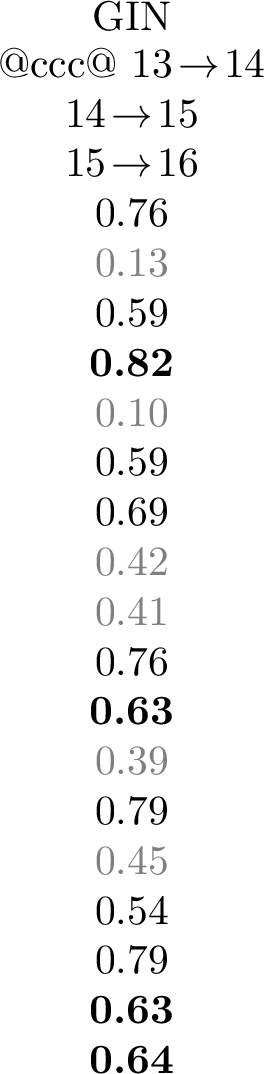
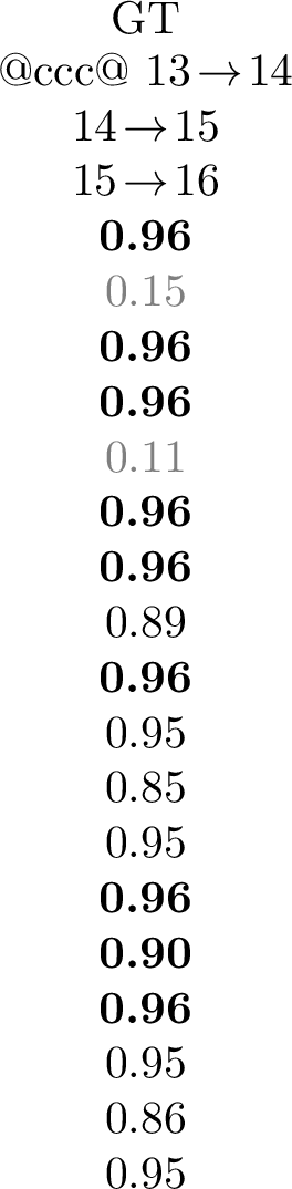
Three features stand out. First, GAT embeddings achieve the highest \(r^2\), indicating strong aggregation of local structure. Second, the \(14\!\to\!15\) experiment shows a striking anomaly: the predictability of \(C_3\) and \(C_4\) collapses, while induced graphlets and \(C_5\) remain highly recoverable. The origin of this effect is unclear and points to a non-trivial structural transition in the dataset. Finally, the high \(r^2\) for \(C_5\), despite no explicit input, indicates that the embeddings capture higher-order, non-local structure.
4 Discussion / Future work↩︎
Our results show that GNNs can identify redundant sectors of the graphical bootstrap while preserving exactness. Working at the \(d\)-graph level limits the reduction, capturing only a subset of vanishing \(f\)-graphs (34% at \(n=16\)). A natural next step is \(f\)-graph-level pruning, which remains a binary task, deciding whether \(c^{(n)}_{a,b}=0\), i.e. on graphs with both numerator and denominator edges. Direct coefficient prediction is a separate and harder problem; nevertheless, at fixed loop order the target is a finite and highly structured set of rational numbers [8]. At 13-loops we expect them to be multiples of \(\frac{1}{8}\) ranging from \(-42\) to \(14\) (stronger constraints can also be conjectured). The coefficient-prediction problem could be then formulated as a structured finite-label task. Finally, we believe this work provides a useful benchmark for learning on purely combinatorial graphs and strengthens the connection between exact results in high-energy physics and machine learning. Code and data are available at code and dataset.
This research was supported in part through the Maxwell computational resources operated at Deutsches Elektronen-Synchrotron DESY, Hamburg, Germany. The authors would like to thank Roi Naveiro Flores for insightful conversation and the beginning of the project. GD is grateful to Nicola Segala for stimulating discussions on graph spectra. PH is supported by STFC Consolidated Grant ST/X000591/1. RA and GD are funded by the Deutsche Forschungsgemeinschaft (DFG, German Research Foundation) under Germany’s Excellence Strategy – EXC 2121 “Quantum Universe” – 390833306.