Variable Bit-width Quantization:
Learning Per-Group Precision for “Bigger-but-Smaller” Language Models
July 03, 2026
Abstract
Low-bit quantization shrinks language models but treats precision as a single global hyper-parameter: every weight is forced to the same bit-width. We introduce Variable Bit-width Quantization (VBQ), a training-time method in which each contiguous group of 64 weights learns its own resolution from \(\{1,2,4,8\}\) bits through a Gumbel-Softmax relaxation, trained jointly with the network by an alternating optimization that gives the precision logits a clean, task-aligned signal. Across decoder-only transformers, VBQ discovers a consistent and strongly heterogeneous allocation, within individual projection types and not merely across layers, that is impossible to express with per-layer methods: \(69\%\) of groups collapse to 1 bit, the language-model head averages \(1.09\) bits, while the first MLP block keeps \(\sim\!2.5\) bits. The discovered pattern is stable enough to be frozen into a fixed recipe and reused without any further search. Using this recipe we demonstrate a “bigger-but-smaller” regime: a 131M-parameter model at \(1.82\) mean bits reaches validation perplexity \(4.2\) on TinyStories, beating a 55M FP16 model (PPL \(4.4\)) while using \(3.8\times\) less storage, and the same recipe lets a \(1.46\)B-parameter model on FineWeb-Edu match a \(593\)M FP16 control at \(\sim\!3.7\times\) less storage (\(2.5\times\) more parameters, \(\sim\!3.7\times\) smaller footprint). Measured as quality-per-byte, VBQ is \(3.9\)–\(8.4\times\) more efficient than FP16. Crucially, the recipe maps directly to packed low-bit storage, so it also accelerates inference: with custom fused dequantize-and-multiply kernels, autoregressive decode, which is memory-bandwidth bound, is faster at equal output, and because the benefit is bandwidth-driven the speedup grows with scale (parity at \(131\)M, \(1.9\times\) at \(1.0\)B, \(4.7\times\) at \(9\)B on Apple silicon). We complement perplexity with a distributional analysis (KL divergence and argmax-flip rate) that reveals a striking mechanism: deeper layers progressively self-heal the quantization error injected by early layers. We delimit the method’s scope honestly: its win is a from-scratch, train-time phenomenon, and scaling the search economically beyond \(1.5\)B parameters and adapting it to pretrained checkpoints remain open. VBQ reframes precision as a learnable, non-uniform resource and shows that spending a fixed bit budget unevenly is materially better than spending it uniformly.
1 Introduction↩︎
The dominant lever for deploying large language models (LLMs) under tight memory budgets is quantization: storing weights at fewer than 16 bits. Almost all deployed schemes (post-training methods such as GPTQ [1] and AWQ [2], and quantization-aware training such as BitNet [3], [4]) fix a single bit-width for (almost) all weights. The schemes that do vary it still fix the allocation by a predetermined rule rather than learning it. Production toolchains such as Unsloth’s dynamic GGUF quants [5] keep salient layers at higher precision as a per-layer, post-training heuristic; NVIDIA’s NVFP4 [6] goes finer, mixing precision within a tensor through 16-element micro-blocks (and reserving a few hand-picked layers for higher precision), and is used both for post-training quantization and for 4-bit pretraining [7]. In every case the bit allocation follows a fixed format or heuristic; it is not a per-group choice the optimization learns during training.
This is a convenient, yet suboptimal modeling choice. Weights in an LLM are not equally important: attention output projections tolerate aggressive compression, while the first feed-forward block and a small set of frequent output-vocabulary rows are far more sensitive. A method that could allocate bits where they matter, at fine granularity and decided by the optimization itself, should dominate any uniform assignment on the quality/size frontier.
A second observation motivates how much precision is actually needed, and is what set this work in motion. In production neural retrieval, the neural hashing that compresses embedding vectors in Algolia’s search stack [8] was originally trained on FP32 vectors and compressed them roughly \(10\times\), to about \(3.2\) bits per dimension, with a change in ranking quality (nDCG) smaller than the noise of the embedding model itself; we later relaxed this to \(4\) bits, but pushing below that range degraded quality quickly. We had treated this as a practical rule of thumb: a trained representation seems to carry on the order of \(3\)–\(4\) useful bits per value, a limit we hit in production, and one that has since surfaced repeatedly in the LLM literature. Apple’s on-device foundation model is independent, production-scale evidence of the same limit: it compresses to a mixed 2-/4-bit scheme averaging \(3.7\) bits-per-weight to match the uncompressed model (and \(3.5\) bits without significant quality loss) [9]. The same threshold recurs in [10], who find \(4\)-bit Pareto-optimal in their \(k\)-bit inference scaling laws. That the largest deployers either still pay for 16-bit weights or accept lossy quantization, yet a carefully mixed scheme reaches \(\sim\!4\) bits without measurable quality loss, is what made the opportunity concrete: there was clearly room to operate near \(4\) bits losslessly; the open question was how to get there. We read this convergence across retrieval, on-device LLMs, and scaling-law analyses as an empirical floor: below roughly \(3.5\)–\(4\) bits per value, information is genuinely lost. VBQ’s “bigger-but-smaller” result is consistent with this floor, but with a crucial twist about how to reach it. The way to hit the floor is not to round every weight to four bits: uniform 4-bit quantization forces a lossy approximation of weights that were never trained for it. It is to spend a comparable total budget differently: distribute it across more, lower-precision weights (in our recipe, an average of \(\sim\!1.8\) bits) so the network learns a representation that lives natively at low bits. The information budget is conserved; the layout is what changes, and, as we show, layout is decisive.
We propose Variable Bit-width Quantization (VBQ). Each group of 64 contiguous weights is given a categorical variable over the candidate bit-widths \(\{1,2,4,8\}\), relaxed with Gumbel-Softmax [11], [12] so it is differentiable. The central difficulty is that the cross-entropy gradient, flowing through the quantizer, overwhelms the bit-budget penalty by two-to-three orders of magnitude, freezing the precision logits at their initialization. We resolve this with two design choices: gradient isolation (the reconstructed weights are detached when computing the bit-selection path, so cross-entropy cannot back-propagate into the precision logits) and an alternating optimization (weight steps and precision steps are interleaved, in the spirit of DARTS [13]). Together these let the logits actually move and commit.
Our key empirical findings are:
A learnable, heterogeneous precision hierarchy emerges (Section 5.1). The network drives \(69\%\) of groups to 1 bit and reserves \(4\)/8 bit for a minority, producing a \(1.78\)-bit mean. The allocation is heterogeneous within projection types, structurally impossible for per-layer mixed-precision methods.
The recipe is the product, not the search (Section 3.4). Bit assignments lock in by \(\sim\!20\%\) of training; freezing them into a fixed recipe (uniform 2 bit blocks, a \(4\)-bit first block, and a frequency-tiered language-model head averaging \(1.18\) bits) reproduces the adaptive result with no Gumbel machinery at deployment.
Bigger-but-smaller (Section 5.2). A 131M model at \(1.82\) bits (29 MB) beats a 55M FP16 model (109 MB) on perplexity, and the same recipe lets a \(1.46\)B model (\(2.5\times\) more parameters) match a \(593\)M FP16 control on FineWeb-Edu at \(\sim\!3.7\times\) less storage.
Depth self-heals quantization error (Section 5.3). A KL-divergence decomposition shows that the representational gap injected by the early 4-bit block is progressively reduced by later 2-bit blocks; the per-position argmax-flip rate vs.FP16 falls monotonically from \(71\%\) to \(28\%\) across depth.
The compression is real at inference time (Section 6). The recipe maps to packed \(\{1,2,4,8\}\)-bit storage that our fused dequantize-and-multiply kernels consume directly, never materializing FP16 weights. Because autoregressive decode is memory-bandwidth bound, the storage win becomes a speed win that grows with model size: from parity at \(131\)M to \(4.7\times\) faster decode at \(9\)B, at bit-exact agreement, on Apple silicon.
VBQ’s win is a from-scratch, train-time phenomenon rather than a free lunch for compressing arbitrary pretrained checkpoints; we make this scope explicit and report the relevant open problems (chiefly economical scaling of the search beyond \(1.5\)B parameters) in Section 7.
2 Related Work↩︎
2.0.0.1 Low-bit and ternary LLMs.
BitNet [3] and BitNet b1.58 [4] train transformers with 1-bit / ternary weights from scratch, fixing the same precision everywhere. ParetoQ [14] unifies 1- to 4-bit QAT and finds that most of the training budget is best spent in full precision with a short low-bit fine-tune, a different regime from our purely from-scratch QAT. Low-bit models have also gained traction at the deployment frontier: the Bonsai family [15] ships open-weight 1-bit and ternary (1.58-bit) models up to \(8\)B parameters with strong reported accuracy-per-byte for on-device inference, obtained by quantization-aware training to a single uniform low-bit format. We note it as evidence of real appetite for the “bigger-but-smaller” regime; VBQ differs in learning a heterogeneous per-group allocation, of which a uniform budget is a special case, so a successfully-learned non-uniform allocation can only match or improve on a uniform one at equal bytes (we do not attempt a head-to-head comparison, as the scale, tokenizer, and evaluation suite differ). VBQ differs from all of these in that the bit-width is not a global constant but a per-group learned quantity.
2.0.0.2 Post-training quantization (PTQ).
GPTQ [1], AWQ [2], SmoothQuant [16], QuIP# [17] and AQLM [18] compress an already-trained model using calibration data, second-order information, or learned codebooks. LLM.int8() [19] keeps a few outlier channels in higher precision via a fixed threshold. Production toolchains increasingly ship per-layer dynamic mixed precision in this PTQ regime: Unsloth’s dynamic GGUF quants [5] leave salient layers at higher precision via an importance heuristic while pushing the rest to low bit-widths: a post-training, per-tensor analogue of the per-group allocation VBQ learns during training. These are complementary to VBQ: they operate after training and at (mostly) fixed, per-layer bit-widths, whereas we learn the allocation during training at per-group granularity.
2.0.0.3 Mixed-precision search.
Learning or searching per-layer bit-widths is well studied for CNNs: HAQ [20] (RL), HAWQ [21] (Hessian), and the differentiable DNAS / EdMIPS family [22], [23]. For LLMs, MixLLM [24] and SliM-LLM [25] allocate precision across output features or groups, but as post-training salience heuristics. The closest in spirit is the differentiable, Gumbel-based CNN search of [22]; VBQ brings this idea to decoder-only LLMs, at per-group (64-weight) granularity, with gradient isolation and alternating optimization that are necessary to make training-time selection work at this scale. To our knowledge, no prior work learns per-group bit-widths jointly during training for LLMs.
2.0.0.4 Concurrent work on differentiable quantization.
Two recent papers apply differentiable discrete relaxations to LLM precision in post-training settings, and clarify what is distinct about VBQ. GSQ [26] uses a Gumbel-Softmax relaxation to jointly learn per-coordinate scalar-grid assignments and per-group scales of an already-trained model, matching trellis-quantized accuracy while staying in a deployment-friendly scalar format; it optimizes a layer-wise reconstruction loss rather than the task loss, and selects grid points rather than power-of-two bit-widths. dMX [27] learns per-layer floating-point (OCP MX) formats via a continuous offset annealed to discrete formats. VBQ is complementary on three axes: it learns integer bit-widths at per-group (64-weight) granularity, from scratch against the task loss, and distills the result into a fixed recipe; the shared lesson across all three is that annealed differentiable relaxations are an effective way to make discrete precision decisions trainable.
2.0.0.5 Scaling laws and the practical precision floor.
[28] and [29] formalize how parameter count trades against precision, and [10] study \(k\)-bit inference scaling and find \(4\)-bit Pareto-optimal. This \(\sim\!4\)-bit regime is borne out in production: Apple’s on-device foundation model [9] compresses to a mixed 2-/4-bit scheme averaging \(3.7\) bits-per-weight that matches the uncompressed model (and \(3.5\) bits without significant quality loss), a deployed mixed-precision system landing at exactly the precision floor that also motivates VBQ (Section 3). Hardware is converging on the same regime: NVIDIA’s NVFP4 [6] is a \(4\)-bit floating-point format with two-level micro-block scaling (a per-\(16\)-value FP8 scale and a per-tensor FP32 scale) that holds under \(1\%\) accuracy loss versus FP8 on some models, but it fixes a single \(4\)-bit format across the network rather than learning where precision is needed. Our “bigger-but-smaller” results are a concrete instantiation of this trade in the per-group mixed-precision setting: rather than round each weight to the \(\sim\!4\)-bit floor, spend a comparable budget on more, lower-precision parameters.
2.0.0.6 Evaluation beyond perplexity.
[30] show that accuracy alone hides large behavioral changes from compression, and advocate KL divergence and flips (answers changing) as distance metrics. We adopt both to audit VBQ (Section 5.3).
3 Method↩︎
3.1 Per-group quantization↩︎
A weight matrix \(W\) is partitioned into contiguous groups of \(G=64\) weights. Each group \(g\) has a symmetric absmax scale \(s_g\) and a bit-width \(b_g\). For a target bit-width \(b\), the quantizer is \[s_g = \frac{\max_{i\in g}|w_i|}{2^{\,b-1}-1},\qquad \hat{w}_i = s_g \cdot \mathrm{clip}\!\Big(\mathrm{round}(w_i/s_g),\, -(2^{\,b-1}-1),\,2^{\,b-1}-1\Big).\] The 1-bit case is handled as sign with a per-group absmean scale, \(\hat{w}_i = \mathrm{sign}(w_i)\cdot\mathrm{mean}_{j\in g}|w_j|\). Gradients pass through the round/clip via the straight-through estimator [31].
3.1.0.1 Why group size matters.
With \(G{=}1\) the scheme is degenerate: for any single weight, \(\hat{w}=\mathrm{round}(w/s)\cdot s = w\) regardless of \(b\), so all bit-widths produce identical outputs and there is nothing to choose. A shared per-group scale (\(G{=}64\)) is what creates a genuine quality/precision trade-off and, empirically, the heterogeneous allocation we observe (Section 5.1).
3.2 Differentiable bit selection↩︎
Each group carries logits \(\boldsymbol{\ell}_g\in\mathbb{R}^{K}\) over the \(K{=}4\) candidates \(\mathcal{B}=\{1,2,4,8\}\). During the selection path we draw a Gumbel-Softmax sample \(\boldsymbol{\pi}_g=\mathrm{softmax}((\boldsymbol{\ell}_g+\boldsymbol{e}_g)/\tau)\) with Gumbel noise \(\boldsymbol{e}_g\) and temperature \(\tau\) annealed from \(5.0\) to \(0.5\), and form the soft-quantized weight as a convex combination of the candidate reconstructions, \(\hat{w}^{\text{soft}}_i = \sum_{k} \pi_{g,k}\,\hat{w}^{(\mathcal{B}_k)}_i\). The expected bit cost of the network is \(\bar{b} = \frac{1}{N}\sum_g \sum_k \pi_{g,k}\,\mathcal{B}_k\), and the training objective is \(\mathcal{L} = \mathcal{L}_{\text{CE}} + \lambda\,\bar{b}\).
3.2.0.1 What the objective optimizes (and why VBQ is not lossless at fixed size).
\(\mathcal{L}\) is a penalty (Lagrangian) objective, not a quality-constrained one: \(\lambda\) is an exchange rate that trades cross-entropy for bits, and each group is compressed until the marginal quality cost of one fewer bit exceeds \(\lambda\). We deliberately choose \(\lambda\) so the mean lands at \(\sim\!1.8\) bits, below the \(3.5\)–\(4\)-bit information floor discussed in the introduction. At a fixed parameter count VBQ is therefore expected to be worse than an FP16 model: pushing precision below the floor genuinely discards information, and this is by design, not a mis-tuned selection. The capacity is recovered not by squeezing each weight but by layout: spending the same total bit budget across more, lower-precision weights that the network learns to use natively (the “bigger-but-smaller” result). This depends on weights co-adapting to their assigned bit-widths during training; it cannot be obtained by lowering the bits-per-weight of an already-trained model, which merely forces a lossy approximation of weights that were never trained for it. In other words, VBQ does not compress a trained network to fewer bits; it starts from a more efficient bit layout chosen for the target accuracy and storage.
3.3 Gradient isolation and alternating optimization↩︎
The naive objective does not work: the cross-entropy gradient reaching \(\boldsymbol{\ell}_g\) through \(\hat{w}^{\text{soft}}\) is \(\sim\!16\times\) larger than the penalty gradient at every temperature, and Adam’s normalization entrenches whichever logit started largest. The logits never move.
We make two changes. (i) Gradient isolation: in the bit-selection path the candidate reconstructions are detached from the weight values (\(\hat{w}^{(\mathcal{B}_k)} = \texttt{detach}(\cdot)\)), so cross-entropy cannot back-propagate into \(\boldsymbol{\ell}_g\); only the bit penalty trains the precision decision. (ii) Alternating optimization (cf.DARTS [13]): we interleave a weight step (update \(W\) on \(\mathcal{L}_{\text{CE}}\) with logits frozen) and a logit step (update \(\boldsymbol{\ell}\) on \(\mathcal{L}_{\text{CE}}+\lambda\bar b\) with \(W\) frozen). This gives the logits a clean, task-aligned signal about how precision affects loss, rather than the contaminated gradient that froze them. With both changes the bit distribution collapses from near-uniform to a committed (entropy \(<\!1\%\)) heterogeneous allocation. Algorithm 1 makes the two steps precise.
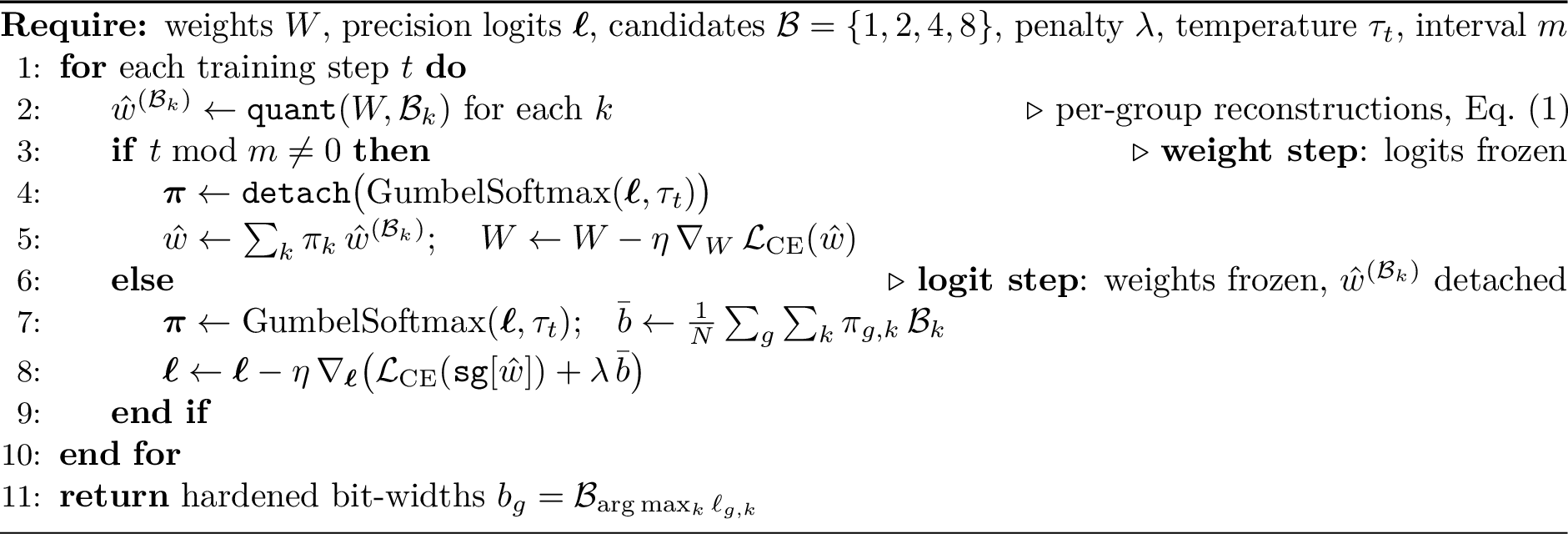
Here \(\texttt{sg}[\cdot]\) (\(\equiv\texttt{detach}\)) is the stop-gradient that implements gradient isolation: in the logit step the reconstructions are held constant so the only path into \(\boldsymbol{\ell}\) is through \(\bar b\) and the explicit dependence of \(\boldsymbol{\pi}\) on \(\boldsymbol{\ell}\).
3.4 From discovery to a fixed recipe↩︎
Because the allocation locks early (Section 5.1), production training does not need the Gumbel machinery at all. We distill the discovered pattern into a fixed VBQ recipe:
First block MLP (
gate/up/down): 4 bit (most sensitive layer).All other attention and MLP projections: 2 bit.
Language-model head: frequency-tiered per-row mixed precision. We count token frequencies in the training corpus, rank the vocabulary in descending order of frequency, and assign bit-widths by rank percentile: top \(0.5\%\) of tokens at 8 bit, next \(1.5\%\) at 4 bit, next \(10\%\) at 2 bit, bottom \(88\%\) at 1 bit (mean \(1.18\) bits). These four cutoffs are not tuned per run; they are chosen once to reproduce the per-row allocation that the adaptive search discovers for the head (Section 5.1).
The recipe is the single most transferable artifact of the method: it requires only a token-frequency table for the head (a single pass over the corpus) and a one-line projection-name map for a new architecture.
4 Experimental Setup↩︎
4.0.0.1 Models and data.
The discovery and ablation studies use nanoGPT-style decoder-only transformers (RoPE [32], SwiGLU [33], weight-tied head) trained on TinyStories [34] (200M tokens, GPT-2 tokenizer [35]). Scale-up experiments use FineWeb-Edu [36] (2B tokens, Qwen tokenizer [37]). Sizes range from 55M to 1.46B parameters.
4.0.0.2 Training.
AdamW (\(\beta=(0.9,0.95)\), weight decay \(0.1\)), cosine schedule \(3\!\times\!10^{-4}\!\to\!3\!\times\!10^{-5}\) with warmup, gradient clip \(1.0\). TinyStories runs use \(35\)K iterations. Storage is reported as the packed weight size at the realized mean bit-width (embedding/head included); “FP16” baselines store every weight in 16 bits. We report validation perplexity (PPL), and for the distributional study, mean token-level KL divergence to an FP16 reference and the argmax-flip rate.
5 Results↩︎
5.1 A learned, heterogeneous precision hierarchy↩︎
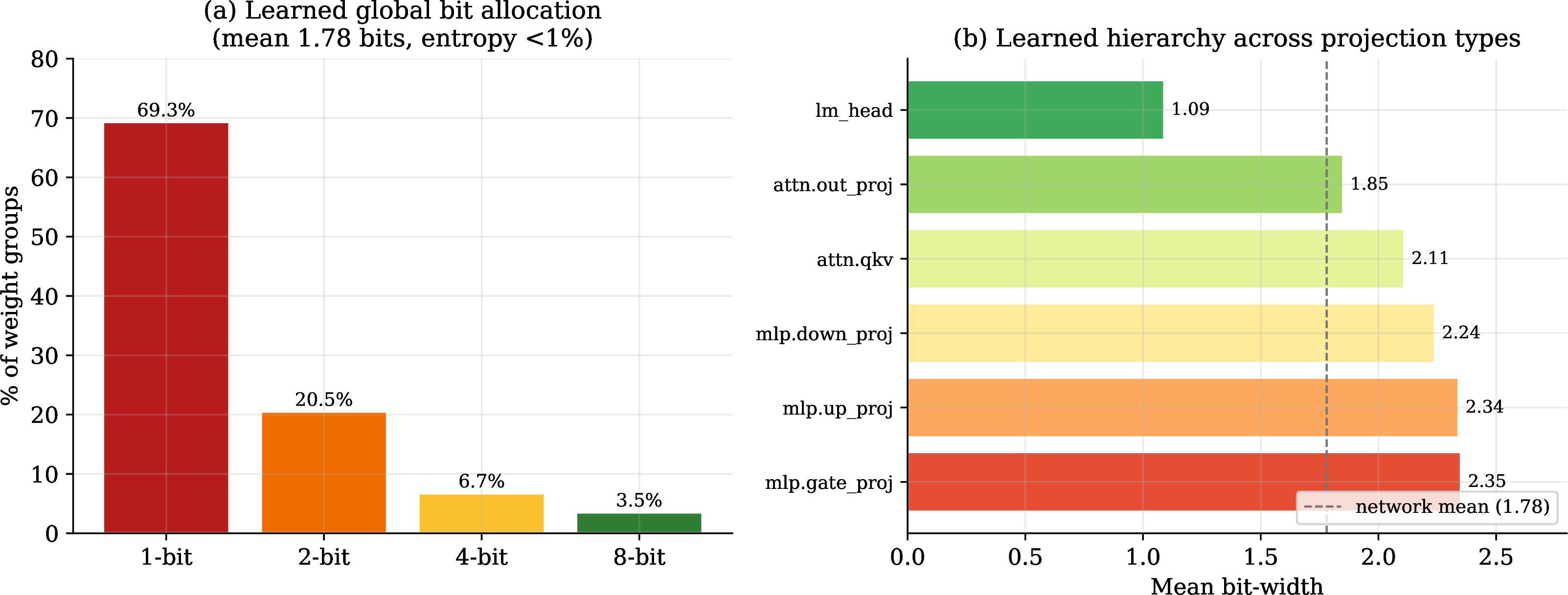
The adaptive pilot (58M, 8 layers, TinyStories) converges to a mean of \(1.78\) bits with a sharply heterogeneous distribution (Figure 2a): \(69.3\%\) of groups choose 1 bit, \(20.5\%\) 2 bit, \(6.7\%\) 4 bit, \(3.5\%\) 8 bit, at near-zero selection entropy. The allocation follows a stable projection-type hierarchy (Figure 2b): the language-model head averages \(1.09\) bits (\(92.5\%\) of its rows are pure 1 bit), attention output projections are the cheapest in-block projection, and the SwiGLU gate/up projections of the first block are the hungriest (up to \(2.5\) bits with \(\sim\!10\%\) 8 bit groups). Crucially, the heterogeneity exists within a projection type, not only across layers, a degree of freedom no per-layer method can use.
The head’s allocation is semantically interpretable: \(4.8\%\) of the \(1000\) most-frequent vocabulary rows contain 8 bit groups versus \(0.06\%\) of the rarest, and the high-precision rows are dominated by function words and punctuation. The same frequency structure is what motivates the recipe’s frequency-tiered head (Section 3.4). Finally, the allocation locks by \(\sim\!10\)K of \(50\)K steps; the remaining \(80\%\) of training only tunes weights within fixed precision, empirical justification for prescribing the recipe directly.
5.1.0.1 The discovery transfers to a different architecture (DeltaNet).
To test whether this hierarchy is an artifact of standard transformers, we re-ran the same Gumbel search on Qwen3.5’s hybrid architecture, in which \(75\%\) of the token-mixing layers are Gated DeltaNet (linear
attention) with non-standard projections (in_proj_qkv, in_proj_z, linear_attn.out_proj) rather than softmax attention. The same projection-type hierarchy emerges, and, counter to our worry that an untested layer
family might need more precision, the DeltaNet projections turn out to be the most compressible in the model: in_proj_qkv selects 1 bit for \(95.7\%\) of its groups, while the precision-hungry
projections are again the value and MLP up/down projections (\(\sim\!70\%\) 1 bit, \(\sim\!30\%\) 2 bit). The ranking is stable across checkpoints and no group demands \(4\)/8 bit by mid-training. The practical payoff is that the recipe needs no architecture-specific retuning: extending it to the new projection names and placing DeltaNet layers at 2 bit is, if anything, conservative.
This discovery run fixes the layout; its quality is then validated by the controlled \(1.0\)B from-scratch comparison against a matched FP16 control (Section 7), and the
same packed model supplies the Qwen3.5 inference measurements (Section 6).
5.2 From adaptive to prescribed, and “bigger-but-smaller”↩︎
Table 1 shows the TinyStories scaling ladder. Three points stand out. First, the search is a one-time cost, not a per-model one: the discovered layout, frozen into the fixed recipe, equals or beats the adaptive pilot with no Gumbel machinery at all. This is the practical crux of the method: the expensive part is discovering where the bits should go, and that needs to happen only once. Once the allocation pattern is known, any new model can be trained at low precision by simply reading off the recipe (a per-projection bit map plus a token-frequency table for the head); no search, no relaxation, no extra hyper-parameters at train time. Every result below the pilot row in Table 1, and the entire \(1.46\)B FineWeb-Edu scale-up, uses the prescribed recipe directly rather than re-running the search. Second, the frequency-tiered head is the single most impactful component: switching the head from uniform 1 bit (008a) to frequency-tiered (008f) improves PPL by \(0.6\) for only \(+0.09\) mean bits. Third, and headline: scaling the model up \(2.4\times\) while staying at \(1.82\) bits yields PPL \(4.2\), which beats the 55M FP16 baseline (PPL \(4.4\)) at \(3.8\times\) less storage (Figure 3 (a)). Every VBQ point lies on or below the FP16 Pareto frontier.
| Model | Params | Mean bits | Val PPL | Storage | \(\Delta\) PPL vs.55M FP16 |
|---|---|---|---|---|---|
| 55M FP16 (baseline) | 55M | 16.0 | 4.4 | 109 MB | n/a |
| 131M FP16 (quality ceiling) | 131M | 16.0 | 3.9 | 262 MB | \(-11\%\) |
| adaptive pilot | 55M | 1.78 | 5.1 | 12 MB | \(+16\%\) |
| uniform | 55M | 1.50 | 5.5 | 10 MB | \(+25\%\) |
| mixed head | 55M | 1.59 | 4.9 | 11 MB | \(+11\%\) |
| \(1.3\times\) scale | 73M | 1.66 | 4.9 | 15 MB | \(+11\%\) |
| \(2.4\times\) scale | 131M | 1.82 | 4.2 | 29 MB | \(\bm{-5\%}\) |
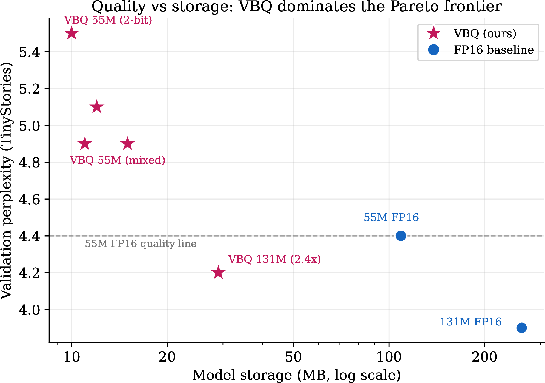
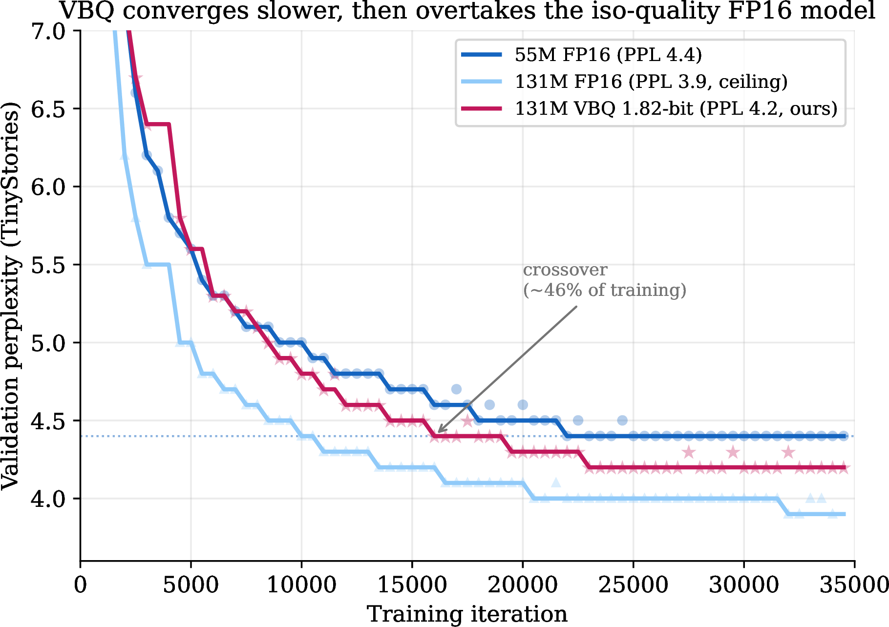
Figure 3: Bigger-but-smaller. (a) Validation perplexity vs.packed storage on TinyStories: every VBQ model (crimson stars) sits on or below the FP16 baselines (blue circles); the \(131\)M VBQ model at \(29\) MB beats the \(55\)M FP16 model at \(109\) MB. (b) Validation perplexity over training for three fixed-architecture \(35\)K-iteration runs. Faint markers are the raw per-eval points; solid lines trace the best perplexity reached so far (a running minimum), which is robust to the transient single-eval spikes visible in the scatter. The \(131\)M VBQ model (\(1.82\) bits) converges more slowly than FP16 but keeps improving after the \(55\)M FP16 model plateaus, crossing its quality line (dotted) at \(\sim\!46\%\) of training and finishing at PPL \(4.2\) vs.\(4.4\).. a — Quality vs.storage frontier., b — Training crossover (real eval logs).
5.2.0.1 Quantization as regularization.
Figure 3 (b) plots the real validation curves. VBQ converges slower than FP16 but keeps improving after FP16 plateaus, crossing the 55M-FP16 quality line near \(46\%\) of training. We attribute this to the low-bit constraint acting as a regularizer: with dropout \(0\), the 131M VBQ model shows a smaller train/val gap than its FP16 twin. A practical consequence is that VBQ runs must not be judged early.
5.2.0.2 Scaling to 1.46B.
On FineWeb-Edu with the Qwen tokenizer, the same recipe applied to a \(1.46\)B-parameter model (\(1.77\) mean bits) reaches a best validation loss of \(2.964\) (PPL \(19.4\)), matching the \(593\)M FP16 control’s best PPL of \(19.4\). The match holds at \(\sim\!3.7\times\) less storage (\(0.32\) vs \(1.19\) GB) with \(2.5\times\) more parameters. The recipe keeps the frequency-tiered head (mean \(1.18\) bits) here too, and its importance is quantified by the TinyStories ablation above: replacing it with a uniform 1 bit head costs \(0.6\) PPL for a saving of only \(+0.09\) mean bits. What matters is not the head’s average bit budget but where those bits go.
5.2.0.3 Quality-per-byte.
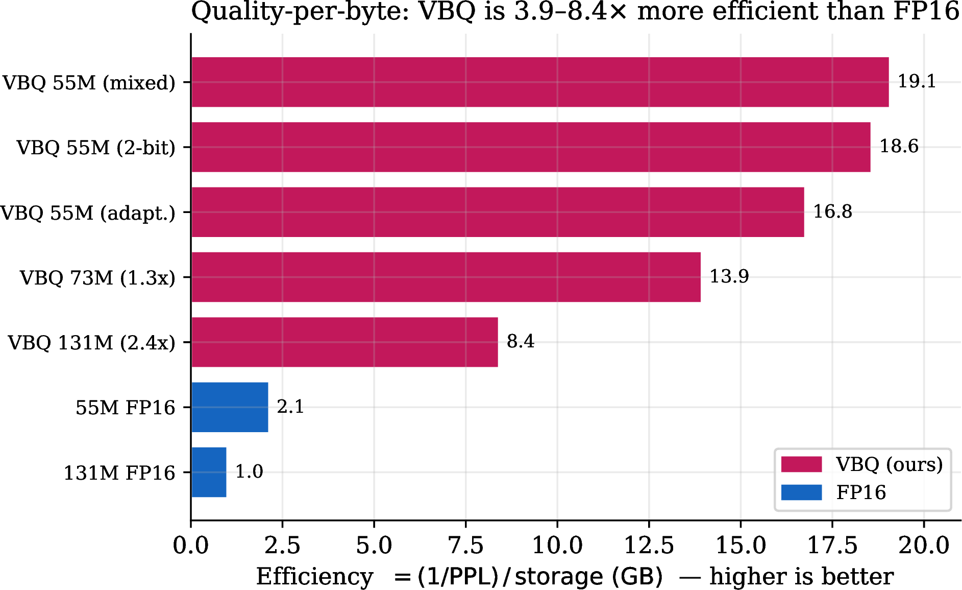
Summarizing with an efficiency metric \((1/\text{PPL})/\text{storage\,(GB)}\), VBQ models are \(3.9\)–\(8.4\times\) more efficient than FP16 across the ladder (Figure 4); the mixed-head 55M model is the most efficient point overall, and there is no overlap between the VBQ and FP16 clusters.
5.3 Distributional analysis: depth self-heals quantization error↩︎
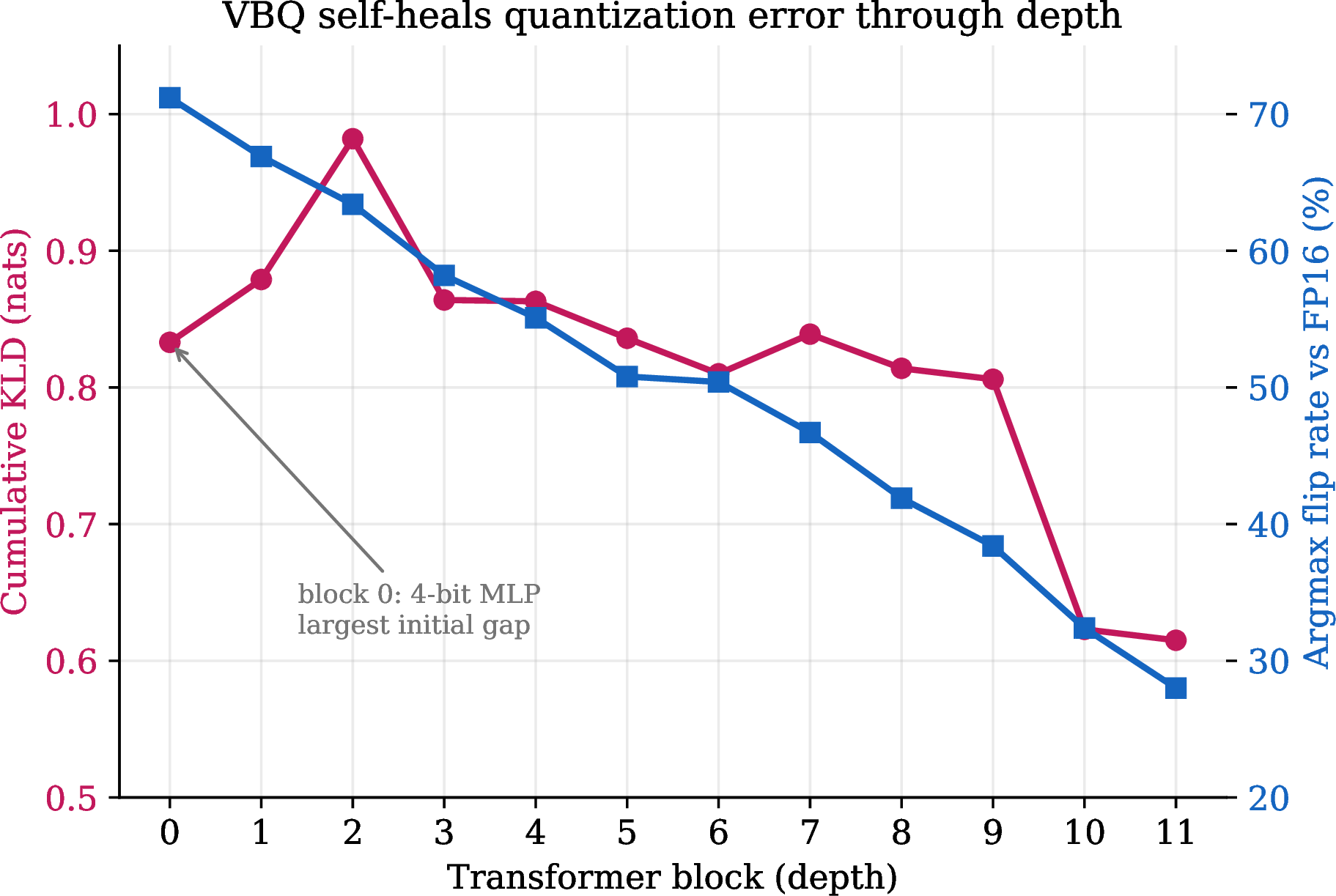
Perplexity can hide behavioral change [30]. We therefore measure mean token-level KL divergence and argmax-flip rate of the 131M VBQ model against a 131M FP16 reference. The full model has mean KLD \(0.21\) nats and an \(18.7\%\) flip rate: at roughly one position in five VBQ selects a different top-1 token, a behavioral cost invisible to PPL, which we report for honesty.
Two findings refine the picture. First, swapping components between the VBQ and FP16 models makes things worse (an FP16 head on VBQ blocks yields KLD \(0.62\), \(3\times\) the full VBQ model), showing the blocks and head co-adapt: the low-bit head works precisely because the blocks learned to produce representations robust to sign-only quantization. Second, a depth probe that projects each block’s hidden state through a single shared FP16 head (excluding VBQ’s own co-adapted head, so blocks are comparable across depth) shows the representational gap is injected early: the \(4\)-bit first block contributes the largest KLD (\(0.83\), \(71\%\) flips) and is then progressively reduced by later \(2\)-bit blocks, the probe’s flip rate falling monotonically from \(71\%\) to \(28\%\) at the final block (Figure 5). This probe sits above the full model’s \(18.7\%\) end-to-end flip rate precisely because it bypasses VBQ’s co-adapted head; restoring that head recovers the \(18.7\%\). VBQ networks effectively learn an error-correcting code over depth. This also explains a negative ablation: adding precision to individual blocks barely moves KLD (\(<\!4.4\%\) for \(+0.34\) bits), because the co-adaptation absorbs whatever precision it is given, making more blocks, not more bits per block, the natural lever.
5.4 Depth vs.width↩︎
The self-healing mechanism suggests depth should be a cheap quality lever, since each extra \(2\)-bit block is nearly free in storage. We tested this directly at fixed width (\(d{=}512\)): adding depth helps consistently but sub-linearly. A 12-layer model improves PPL by \(5\)–\(6\%\) over 8 layers (\(4.9\!\to\!4.6\)), but a 26-layer model plateaus at \(4.77\), far short of the \(\sim\!4.3\) a naive depth extrapolation predicts, and worse per parameter than going wider. Pure depth is therefore not a substitute for width: the headline \(131\)M result wins by being both wider and deeper, not deeper alone.
6 Inference: storage savings become speed↩︎
A learned bit budget is only useful if it survives to deployment. Because autoregressive decode at batch size 1 is memory-bandwidth bound (each generated token must stream every weight from memory through the arithmetic units), a model that stores its weights in fewer bits also reads fewer bytes per token, and decodes faster in direct proportion, provided the weights are never expanded to FP16 in memory.
6.0.0.1 Fused kernels over packed weights.
We implement custom fused dequantize-and-multiply GEMV kernels (Metal for Apple silicon, CUDA for NVIDIA) with a specialization per bit bucket \(\{1,2,4,8\}\). Each kernel loads the packed low-bit bytes for a group, expands them to FP16 in registers using the per-group scale, and accumulates the matrix–vector product, so the full-precision weight matrix is never materialized in memory and the bandwidth saving is realized end to end. The mixed-precision head is stored as a small number of frequency-grouped row buckets.
6.0.0.2 The speedup grows with model size.
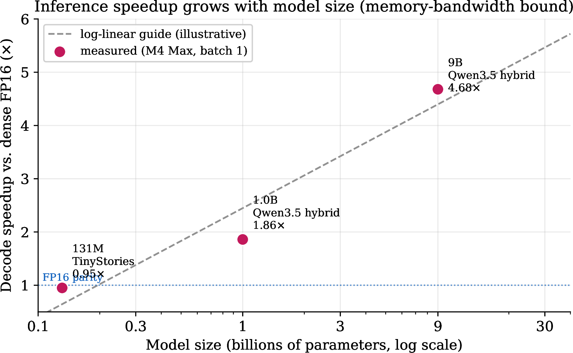
Because the benefit is bandwidth-driven, it appears only once weight traffic dominates; i.e., it scales with model size (Figure 6). Table 2 reports the same-weights
comparison (identical model and runtime; the FP16 baseline is produced by dequantizing the VBQ weights into dense FP16, so only the weight representation differs) at batch 1 on an Apple M4 Max, as the median of repeated runs. At \(131\)M the model is small enough that per-token overhead, not bandwidth, dominates, so VBQ runs at parity (\(0.95\times\)) and the win is purely the \(\sim\!2\times\) smaller memory footprint. By \(1.0\)B decode is \(1.86\times\) faster, and by \(9\)B it is \(4.68\times\) faster (\(135\) vs.\(29\) tok/s), while also fitting in \(3.8\) GB instead of \(17\) GB of peak memory, i.e.running comfortably where the FP16 model is far heavier. The \(1.0\)B/\(9\)B runs use mlx-lm’s generate_step (the real
async_eval decode path); the \(131\)M run uses our fused-kernel greedy decode. VBQ reproduces the dense-FP16 model’s outputs to numerical parity (verified separately: Pearson
correlation \(1.00000\), identical top-1 token), so these are speedups at equal output, not an accuracy/speed trade.
| Linear weights | Peak memory | Decode tok/s | ||
| Model | Params | FP16 \(\to\) VBQ | FP16 \(\to\) VBQ | FP16 \(\to\) VBQ(speedup) |
| TinyStories LM | 131M | \(324\to117\) MB | \(350\to180\) MB | \(592\to564\)(\(0.95\times\)) |
| Qwen3.5 hybrid | 1.0B | \(1503\to240\) MB | \(1845\to592\) MB | \(232\to432\)(\(\bm{1.86\times}\)) |
| Qwen3.5 hybrid | 9B | \(15859\to2528\) MB | \(17052\to3783\) MB | \(29\to135\)(\(\bm{4.68\times}\)) |
The \(9\)B row benchmarks decode speed only; the quality of that particular from-scratch run is a separate, unresolved matter (Section 7), but the packed model is architecturally representative, so it is a valid measurement of how the inference benefit scales.
6.0.0.3 Granularity is deployment-friendly.
We quantize contiguous \(64\)-weight groups (rather than per-channel or per-tensor) because a single shared scale over a short contiguous run is what creates a local quality/precision trade-off (Section 3) while still packing into aligned byte boundaries. Two practical details keep the packed model fast. First, the deployed artifact is the recipe, which is near-uniform per projection type (mostly 2 bit, a 4 bit first block, a tiered head) rather than a fully heterogeneous per-group map, so a kernel dispatches one bit bucket per projection, not one per group. Second, the fastest decode GEMV requires the contracted dimension to be a multiple of \(512\); we zero-pad MLP intermediates to satisfy this (the padded channels are mathematically inert: \(\mathrm{silu}(0)\cdot u = 0\)), recovering a \(1.67\times\) kernel speedup that would otherwise be lost on awkward shapes such as Qwen’s \(8960\)-wide MLP. An export-time check validates this contract.
7 Limitations and Open Problems↩︎
We state the method’s scope plainly, and separate what we have shown from what remains open.
7.0.0.1 Economical scaling beyond 1.5B is the main open problem.
Our positive quality results run from 55M to \(1.46\)B parameters; economically validating the recipe beyond that remains open. A separate controlled \(1.0\)B gate run on Qwen3.5’s hybrid architecture (\(1006.7\)M total parameters) used a different tokenizer, a matched FP16 control, and \(\geq\!99\%\) quantization coverage, but was deliberately short at \(0.37\) tokens/parameter, about \(4\times\) fewer than the \(\sim\!1.4\) used in the matched FineWeb runs. This was by design: it is a cheap transfer probe to check that the recipe carries to a hybrid architecture at all, not a run to convergence; full matched runs at this scale are precisely the economics we flag as unsolved. Even so, at the stopped checkpoint VBQ was \(+0.28\) nats behind FP16 (\(1.33\times\) PPL) with the gap still narrowing over the final third (\(0.36\!\to\!0.28\) nats), consistent with VBQ’s known slower convergence and showing no sign of a scaling ceiling. This \(1.0\)B gate is not numerically comparable to the \(1.46\)B FineWeb-Edu standard-transformer result (architecture, tokenizer, and token budget all differ), so it probes recipe transfer to a harder hybrid setting rather than contradicting the standard-transformer parity result. We also attempted a single \(9\)B from-scratch knowledge-distillation [38] run, but it was confounded and we do not draw conclusions from it: a coverage bug left \(18\%\) of parameters (non-standard hybrid-attention projections) unquantized so the realized precision was not the intended \(1.77\) bits, and it was trained at only \(0.27\) tokens/parameter (about \(5\times\) under the \(\sim\!1.4\) used by our successful runs) on an untested architecture family. A properly-tokened \(9\)B run (estimated \(\sim\!12\)B tokens) was beyond our compute budget. Nothing in our results suggests the method stops scaling; closing the \(\ge\!9\)B regime economically, and clearing the strong-baseline bar at that scale (a \(4\)-bit PTQ of a same-storage teacher), is future work rather than a counter-result.
7.0.0.2 Frozen-base depth-boosting does not add useful capacity.
Motivated by self-healing, we tried to add low-bit correction blocks onto a converged 12-layer model with the base frozen (a gradient-boosting analogy with near-identity initialization). Training loss improved but validation did not (a classic overfit signature, with intermittent instability); the added blocks fit batch idiosyncrasies rather than generalizable residual signal. At least with a small frozen base, post-hoc correction depth is not a shortcut to the from-scratch win. We suspect a larger pretrained base would not rescue this either: the “bigger-but-smaller” win comes from weights co-adapting to low bit-widths during training, which a frozen or otherwise pretrained base cannot inherit; and indeed, separate attempts to search per-group bit-widths post-hoc on frozen pretrained weights were dominated by trivial uniform 4-bit. The more promising direction is therefore to scale the from-scratch “bigger-but-smaller” recipe itself, not to adapt pretrained bases.
7.0.0.3 Scope.
Our positive results are on English next-token modeling up to \(1.5\)B parameters, on two corpora, with perplexity and KL/flip metrics; we do not report downstream task suites (MMLU/GSM8K/etc.) at scale. The method targets the train-from-scratch setting; it is not, on current evidence, a superior post-training compressor competing with GPTQ, AWQ, QuIP#, or AQLM at \(4\) bits.
8 Conclusion↩︎
VBQ treats numerical precision as a per-group, learnable resource rather than a global constant. A Gumbel-Softmax relaxation, made trainable by gradient isolation and alternating optimization, discovers a strongly heterogeneous bit-width hierarchy that is stable enough to freeze into a reusable recipe. The central lesson is that spending a fixed bit budget unevenly is materially better than spending it uniformly: with the recipe, models become simultaneously larger in parameter count and smaller in storage than their FP16 equivalents, and \(3.9\)–\(8.4\times\) more efficient in quality-per-byte. This is consistent with the \(\sim\!4\)-bit compression floor that recurs across independent settings [8]–[10]: VBQ reaches that floor not by rounding each weight to four bits, but by redistributing a comparable budget across more, lower-precision weights. This is not only a storage result: the same packed weights decode faster through fused low-bit kernels, increasingly so with scale (up to \(4.7\times\) at \(9\)B), because decode is memory-bandwidth bound. The three wins compound rather than trade off: a VBQ model can hold more parameters, occupy about a quarter of the storage, and decode several times faster than its FP16 counterpart at once, and because the speedup is bandwidth-driven it grows with model size, so the combination is most valuable exactly where serving cost dominates. A KL-divergence analysis reveals why the aggressive bit budget is survivable: depth self-heals the error injected by early layers, so the network effectively learns an error-correcting code that lets a non-uniform allocation pay off. The remaining frontier is to push the from-scratch “bigger-but-smaller” recipe economically past \(1.5\)B parameters. Precision should not be treated merely as a post-training tuning knob, but as a structural design input to training itself: choosing the bit layout up front yields faster, more efficient models that can operate closer to the quality/size Pareto frontier out of the box.
8.0.0.1 Reproducibility.
All figures are regenerated from the released training logs and tabulated results by the script in paper/figures/.
References↩︎
UD-* series): salient layers are retained at higher precision via an importance heuristic while the rest are pushed to low bit-widths.