1 Introduction↩︎

Many online decision-making problems, such as online ad display and contextual treatment assignment, involve choosing among actions represented by feature vectors that can include both the current context and action-specific information. In these applications, feasible actions are naturally round-specific: they depend on the current user or patient and, in ad display, on the ad impressions currently available. Linear bandits [1], [2] provide a standard model for such problems: each feasible decision is represented by a feature vector, and its expected reward is modeled as the inner product between this feature vector and an unknown parameter vector. The standard performance measure for a policy is regret, which compares the policy’s cumulative reward with that of a benchmark. In the classical stationary model, the unknown parameter is fixed, and this benchmark selects the best feasible decision under the fixed parameter at each round.

In many applications, however, the relationship between actions and expected rewards may drift over time: user preferences may evolve, market conditions may shift, and patient responses to treatments may change. This concern has motivated a broad literature on non-stationary stochastic optimization and non-stationary bandit learning [3]–[8]. The non-stationary linear bandit model captures such drift by allowing the reward parameter to change across rounds. Formally, consider an online decision-making problem over \(T\) rounds: at each round \(t\), the learner observes a feasible decision set \(\mathcal{A}_t\subseteq\mathbb{R}^d\), chooses an action \(a_t\in\mathcal{A}_t\), and receives a reward with conditional mean \(\langle a_t,\theta_t\rangle\), where \(\theta_t\) is the current reward parameter. Following [7], the non-stationarity of a problem instance is measured by the path length of the reward-parameter sequence, \(P_T:=\sum_{t=1}^{T-1}\|\theta_{t+1}-\theta_t\|_2\). For a policy \(\pi\), with \(a_t\) denoting its round-\(t\) action, define the dynamic regret \[\operatorname{Reg}_T(\pi) := \mathbb{E}\sum_{t=1}^T \left[ \max_{a\in\mathcal{A}_t}\langle a,\theta_t\rangle - \langle a_t,\theta_t\rangle \right],\] which compares the learner’s expected reward at each round with that of the best feasible action under the current parameter. The goal is to achieve small dynamic regret when \(P_T\) is moderate.

Several works study non-stationary linear bandits under path-length constraint [7], [9]–[11]. However, existing rate-optimal approaches for non-stationary linear bandits do not fully cover the case of round-specific feasible decision sets. [7] obtain the \(\widetilde{O}(T^{2/3}P_T^{1/3})\) upper bound in this regime by requiring all feasible actions to lie on a fixed set of orthogonal directions, and establish the corresponding \(\Omega(T^{2/3}P_T^{1/3})\) lower bound. The orthogonal-direction assumption can be restrictive in contextual applications, where users, ad opportunities, and patient-treatment pairs are often described by context-dependent attributes, leading to feature vectors with shared structure rather than scalar multiples of fixed orthogonal basis directions. This restriction leaves open the problem of achieving the optimal \(T^{2/3}P_T^{1/3}\) dynamic-regret dependence for non-stationary linear bandits with general round-specific feasible decision sets [10], [11].

Our contributions. We show that the optimal \(T^{2/3}P_T^{1/3}\) dynamic-regret dependence can be achieved for round-specific decision sets without the orthogonal-direction assumption. We prove this in two settings: general compact decision sets and \(K\)-armed contextual linear bandits.

The key idea is a local misspecification reduction: parameter drift within each block is treated as model misspecification, so the desired dynamic-regret rate follows from blockwise regret guarantees that adapt to the misspecification level. The reduction is based on the following blockwise bound. On a block \(\mathcal{I}=\{\tau,\ldots,\tau+n-1\}\), using \(\theta_\tau\) as the block comparator gives \[\sup_{t\in\mathcal{I}}\sup_{a\in\mathcal{A}_t} |\langle a,\theta_t-\theta_\tau\rangle| \le L P_{\mathcal{I}},\] where \(L\) upper bounds the norms of feasible actions and \(P_{\mathcal{I}}\) denotes the path length of the parameter sequence restricted to block \(\mathcal{I}\). In general, if a block comparator \(\bar\theta\) has uniform error at most \(\varepsilon\) on \(\mathcal{I}\), dynamic regret on the block is bounded by two terms: regret against the blockwise fixed-parameter benchmark induced by \(\bar\theta\), and an approximation term \(O(n\varepsilon)\). The first term is precisely the regret of a misspecified linear bandit on the block, with misspecification level \(\varepsilon\). Consequently, a guarantee of order \(\widetilde{O}(\sqrt n+n\varepsilon)\) yields the block dynamic-regret bound \(\widetilde{O}(\sqrt n+nLP_{\mathcal{I}})\) after taking \(\varepsilon=LP_{\mathcal{I}}\). Restarting on blocks of length \(\Delta\) and summing over blocks gives the tradeoff \(\widetilde{O}(T/\sqrt\Delta+\Delta P_T)\). Choosing the optimal \(\Delta\) gives the \(\widetilde{O}(T^{2/3}P_T^{1/3})\) dependence.

We obtain the following guarantees in two settings:

• General compact decision sets. For linear bandits with general compact, adaptive non-anticipating decision sets and an oblivious parameter path, Theorem 1 shows that a restarted CORRAL aggregation of SquareCB.Lin+ bases [12] achieves the expected dynamic-regret bound \[\widetilde{O}\!\left( d\sqrt T + L^{1/3}d^{5/6}T^{2/3}P_T^{1/3} \right).\] Thus the method attains the optimal \(T^{2/3}P_T^{1/3}\) dynamic-regret dependence, matching the lower-bound dependence of [7] while allowing general round-specific compact action sets beyond the orthogonal-direction structure.

• \(K\)-armed contextual linear bandits. For \(K\)-armed contextual linear bandits under an oblivious adversary, with \(\Lambda_K:=1+\log K\), Theorem 2 shows that restarting SupLinUCB [2] achieves the expected dynamic-regret bound \[\widetilde{O}\!\left( \sqrt{dT}\,\Lambda_K + \sqrt d\,\Lambda_K^{5/6}T^{2/3}P_T^{1/3} \right).\] This again matches the optimal dependence on \(T\) and \(P_T\), as certified by Proposition [prop:finite-k-lower-bound].

Unlike the original SquareCB.Lin+ misspecification guarantee of [12], which considers oblivious sequences, our setting allows adaptive non-anticipating decision sets. This requires an additional conditional argument. On each block, the comparator and misspecification radius are fixed before the within-block randomization. Consequently, the misspecification-dependent terms remain predictable, and the SquareCB.Lin+ base and CORRAL master guarantees can be invoked conditionally. If \(P_T\) is unknown, a Bandit-over-Bandit layer can remove this tuning at the usual parameter-free cost [7], [10].

Related work and positioning. Restarting, sliding-window, and weighted-estimation methods are common tools for non-stationary bandits [4], [7], [9]–[11]. For non-stationary linear bandits, recent work identifies a gap between simple forgetting analyses and the \(T^{2/3}P_T^{1/3}\) lower bound when feasible sets are round-specific [10]. Our work addresses this gap: round-specific feasible sets can be handled directly by reducing within-block parameter drift to bounded linear misspecification. The proof is built on this connection between non-stationary linear bandits and misspecified linear bandits, using misspecification-adaptive linear-bandit guarantees [12], [13] to remove the orthogonal-structure assumption on round-specific action sets.

Organization. The rest of the manuscript is organized as follows. Section 2 introduces the model and block notation. Section 3 proves the dynamic-regret guarantee for general linear bandits with adaptive non-anticipating decision sets. Section 4 develops restarted SupLinUCB and its dynamic-regret guarantee for \(K\)-armed contextual linear bandits. Section 5 concludes this manuscript.

2 Problem Setting↩︎

We consider a non-stationary contextual linear bandit over \(T\) rounds. At each round \(t\), the learner observes a nonempty feasible decision set \(\mathcal{A}_t\subseteq\mathbb{R}^d\). We identify each feasible action with its feature vector. The learner selects an action \(a_t\in\mathcal{A}_t\) and observes a scalar reward \(r_t=r_t(a_t)\). There is an unknown parameter sequence \(\theta_1,\ldots,\theta_T\in\mathbb{R}^d\), and the conditional mean reward is linear: \(\mu_t(a)=\langle a,\theta_t\rangle\) for \(a\in\mathcal{A}_t\). When a norm bound \(S\) on the parameters is imposed, we write \(\Theta:=\{\theta\in\mathbb{R}^d:\|\theta\|_2\le S\}\); in the \(K\)-armed setting below we use the same notation with \(S=1\).

Histories. Let \(\mathcal{H}_{t-1}\) denote the interaction history through the end of round \(t-1\). When adaptive decision sets are allowed, we also write \(\mathcal{G}_t\) for the round-\(t\) \(\sigma\)-field after the current decision set and the learner’s action distribution have been determined, but before the action is sampled and before the reward noise is realized.

Dynamic regret. For a policy \(\pi\), let \(a_t\) be the action selected by \(\pi\) at round \(t\), and let \(a_t^\star\) be an optimal action at round \(t\), i.e., \(a_t^\star\in\argmax_{a\in\mathcal{A}_t}\mu_t(a) =\argmax_{a\in\mathcal{A}_t}\langle a,\theta_t\rangle\). The expected dynamic regret of \(\pi\) is \[\operatorname{Reg}_T(\pi) := \mathbb{E}\left[ \sum_{t=1}^T \left( \langle a_t^\star,\theta_t\rangle - \langle a_t,\theta_t\rangle \right) \right].\] When the policy or algorithm is clear from context, we write \(\operatorname{Reg}_T\) for \(\operatorname{Reg}_T(\pi)\).

\(K\)-armed contextual specialization. The \(K\)-armed contextual linear-bandit setting considered by [2] is the special case \(\mathcal{A}_t=\{x_t(i):i\in[K]\}\). The learner chooses \(i_t\in[K]\), equivalently \(a_t=x_t(i_t)\), and \(\mu_t(i):=\mu_t(x_t(i))\).

Block notation. For an interval \(\mathcal{I}=\{\tau,\ldots,\tau+n-1\}\), write \(\mathbb{E}_\tau[\cdot]:=\mathbb{E}[\cdot\mid\mathcal{H}_{\tau-1}]\), where \(\mathcal{H}_{\tau-1}\) is the history before the block starts. The dynamic regret on block \(\mathcal{I}\) is \(\operatorname{Reg}(\mathcal{I}) := \sum_{t\in\mathcal{I}} \left( \langle a_t^\star,\theta_t\rangle - \langle a_t,\theta_t\rangle \right)\).

3 General Linear Bandits with Adaptive Non-Anticipating Decision Sets↩︎

In this section we consider the setting in which the parameter path \((\theta_t)_{t=1}^T\) is fixed before interaction begins and is independent of the learner’s randomization and reward noise. The decision sets, however, may be adaptive but non-anticipating: at each round \(t\), \(\mathcal{A}_t\) may depend on \(\mathcal{H}_{t-1}\), but it is fixed before any current-round learner randomization is drawn and before the reward noise is realized. Equivalently, after \(\mathcal{A}_t\) and the learner’s action distribution have been determined, \(\mathcal{G}_t\) contains these quantities but not the round-\(t\) action sample. The technical point, relative to the oblivious-sequence analysis in [12], is that our block proof is written conditionally on this round-\(t\) \(\sigma\)-field, which allows adaptively generated decision sets.

Allowing such adaptivity is important in operational problems where the feasible actions at a round are shaped by past decisions, resource states, and observed feedback. Online ad display provides one example. For a given impression, ad eligibility may depend on past serving decisions through frequency caps, exposure limits, campaign pacing or delivery constraints, and advertiser-side resource availability. It may also depend on feedback observed before the current impression, such as past clicks, conversions, negative feedback, or other engagement signals. Thus the model allows the feasible action set to respond to the learner’s previous actions and observations, while requiring it to be fixed before the current reward realization.

Unbounded conditionally sub-Gaussian rewards can be clipped and rescaled, incurring only standard logarithmic factors. Thus, we state the formal results under bounded rewards.

Algorithmic idea. Following the restarting viewpoint of [4], the algorithm partitions the horizon into blocks and restarts a CORRAL master [12], [14] over SquareCB.Lin+ bases. The CORRAL layer randomizes over base learners and competes with the best base learner in hindsight, up to its aggregation cost. In our use of CORRAL, the bases are indexed by a geometric grid of candidate misspecification levels. On each block, the unknown parameter drift acts as an unknown misspecification level, and the grid contains a candidate within a constant factor of this level.

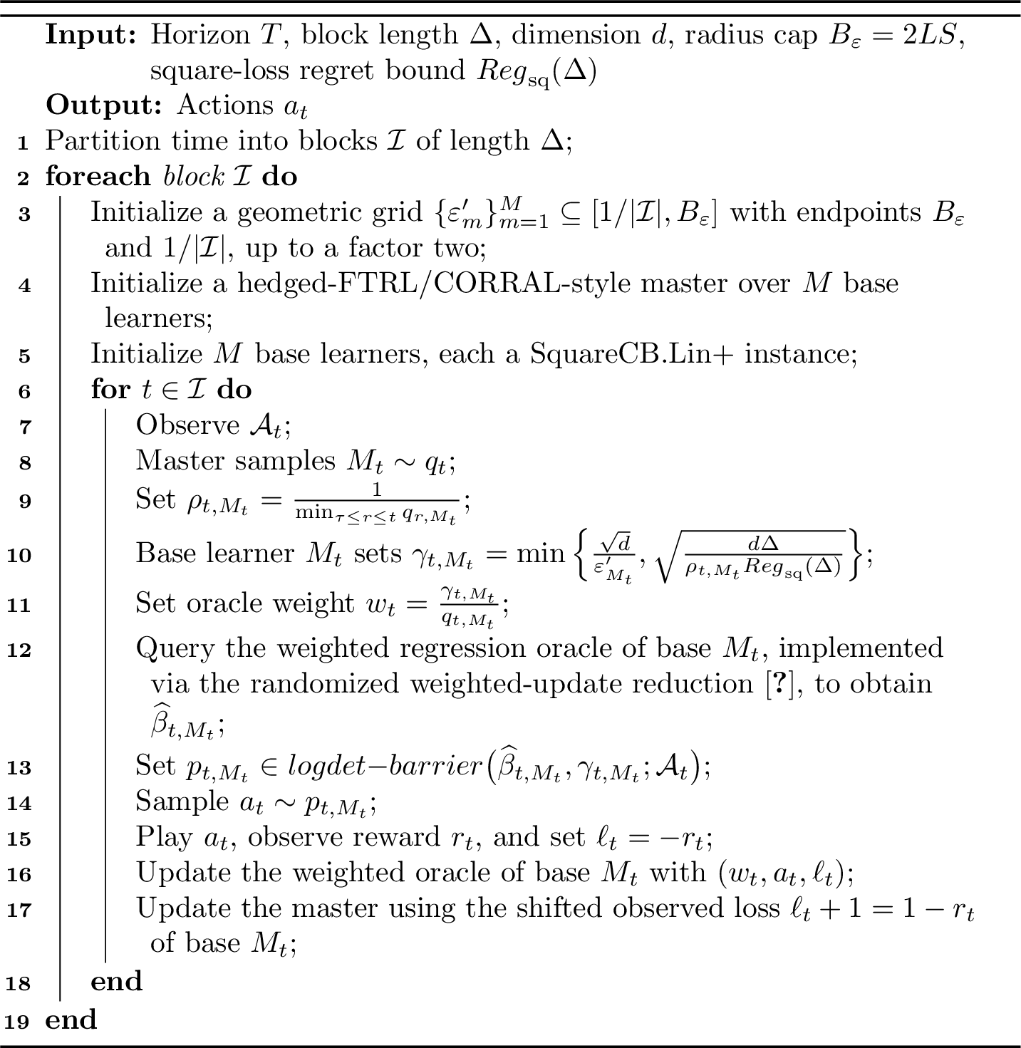
We now describe the grid, oracle interface, and sampling rule used in Algorithm 1. On a block of length \(n\), let \(B_\varepsilon:=2LS\) and use a geometric grid \(\{\varepsilon'_m\}_{m=1}^M\subseteq[1/n,B_\varepsilon]\), with largest point \(B_\varepsilon\), smallest point \(1/n\), and common ratio two. For base \(m\), set the exploration parameter \[\gamma_{t,m} = \min\left\{ \frac{\sqrt d}{\varepsilon'_m}, \sqrt{\frac{dn}{\rho_{t,m}\operatorname{Reg}_{\rm sq}(n)}} \right\}.\] Although Algorithm 1 invokes a weighted square-loss oracle, the randomized reduction of [12] allows this interface to be implemented using an unweighted online square-loss regression oracle. For the bounded linear square-loss class considered here, the online Newton step of [15] gives \(\operatorname{Reg}_{\rm sq}(n)=\widetilde{O}(d)\).

For the SquareCB.Lin+ sampling rule, let \(\Delta(\mathcal{A})\) be the set of distributions on \(\mathcal{A}\), and for \(p\in\Delta(\mathcal{A})\) write \(\bar a_p:=\mathbb{E}_{a\sim p}[a]\) and \(H_p:=\mathbb{E}_{a\sim p}[aa^\top]\). Given \((\widehat\beta,\gamma,\mathcal{A})\), the base chooses any minimizer of \[\label{eq:logdet-barrier-definition} \begin{align} \argmin_{p\in\Delta(\mathcal{A})} \Bigl\{\langle \bar a_p,\widehat\beta\rangle-\gamma^{-1}\log\det(H_p-\bar a_p\bar a_p^\top) \Bigr\}. \end{align}\tag{1}\] We write \(\operatorname{logdet\text{-}barrier}(\widehat\beta,\gamma;\mathcal{A})\) for this set of minimizers.

At round \(t\), the master samples an index \(M_t\sim q_t\) and follows base learner \(M_t\). Let \(Z_{t,m}:=\mathbf{1}\{M_t=m\}\). On a block \(\mathcal{I}=\{\tau,\ldots,\tau+n-1\}\), define \(\rho_{t,m}:=1/\min_{\tau\le r\le t}q_{r,m}\) and \(\rho_{\mathcal{I},m}:=\max_{t\in\mathcal{I}}\rho_{t,m}\). The master outputs an interior distribution, so \(q_{t,m}>0\). If base \(m\) is selected, its oracle weight is \(w_{t,m}:=\gamma_{t,m}/q_{t,m}\). Each base \(m\) proposes an action distribution \(p_{t,m}\). The selected base therefore proposes \(p_{t,M_t}\), and the learner samples \(a_t\sim p_{t,M_t}\).

Lemma 1 gives the block regret guarantee for Algorithm 1 under the fixed-radius misspecification condition above.

Let \(\mathcal{G}_t\) be the round-\(t\) \(\sigma\)-field defined above. Let \(\ell_t=-r_t(a_t)\) denote the observed loss supplied to the selected base. The master receives the shifted loss \(\ell_t+1=1-r_t(a_t)\). Under the mean-loss convention \(L_t(a)=-\langle a,\theta_t\rangle\), we have \(\mathbb{E}[\ell_t\mid \mathcal{G}_t,M_t,a_t]=L_t(a_t)\). Then \(a_t^\star\in\argmax_{a\in\mathcal{A}_t} \langle a,\theta_t\rangle =\argmin_{a\in\mathcal{A}_t}L_t(a)\), and therefore \[L_t(a_t)-L_t(a_t^\star) = \langle a_t^\star,\theta_t\rangle - \langle a_t,\theta_t\rangle .\] Thus the reward-regret on the block is exactly the loss-regret for the losses \(L_t\).

We condition on \(\mathcal{F}_{\mathcal{I}}\), the \(\sigma\)-field just before the first within-block randomization. Under Assumption 4, the comparator \(\theta_{\mathcal{I}}^\star\) is fixed under this conditioning. Put \(\beta_{\mathcal{I}}^\star:=-\theta_{\mathcal{I}}^\star\). Then, for every \(t\in\mathcal{I}\), \[\begin{align} &\sup_{a\in\mathcal{A}_t} \left| L_t(a)-\langle a,\beta_{\mathcal{I}}^\star\rangle \right|\\ =& \sup_{a\in\mathcal{A}_t} \left| \langle a,\theta_t\rangle - \langle a,\theta_{\mathcal{I}}^\star\rangle \right|\le \bar\varepsilon_{\mathcal{I}}. \end{align}\] The proof follows the structure of the oblivious-sequence argument of [12], with the sequence-level comparator and misspecification radius replaced by the fixed block pair \((\beta_{\mathcal{I}}^\star,\bar\varepsilon_{\mathcal{I}})\). For each \(t\in\mathcal{I}\), the residual \[e_t(a):=L_t(a)-\langle a,\beta_{\mathcal{I}}^\star\rangle\] is \(\mathcal{G}_t\)-measurable as a function of \(a\in\mathcal{A}_t\). Moreover, \(\sup_{a\in\mathcal{A}_t}|e_t(a)|\le\bar\varepsilon_{\mathcal{I}}\).

The learner’s regret under CORRAL decomposes into two parts: master regret and base regret. The base-regret term for base \(m\) takes the following importance-weighted form: \[\operatorname{Reg}_{\rm Imp}^m(\mathcal{I}) := \mathbb{E}_\tau\!\left[ \sum_{t\in\mathcal{I}} \frac{Z_{t,m}}{q_{t,m}} \bigl( L_t(a_t)-L_t(a_t^\star) \bigr) \right].\] Here \(Z_{t,m}/q_{t,m}\) is the importance weight that makes the selected rounds for base \(m\) an unbiased conditional estimate of the loss-regret of the counterfactual actions proposed by that base.

For every bounded random function \(\phi_t\) on \(\mathcal{A}_t\) whose values are \(\mathcal{G}_t\)-measurable, \[\label{eq:conditional-importance-weighting} \mathbb{E}\!\left[ \frac{Z_{t,m}}{q_{t,m}}\phi_t(a_t) \,\middle|\,\mathcal{G}_t \right] = \mathbb{E}_{a\sim p_{t,m}}[\phi_t(a)] .\tag{2}\] Because \(\beta_{\mathcal{I}}^\star\) and \(\bar\varepsilon_{\mathcal{I}}\) are fixed under the block conditioning, the residual-dependent functions used below are \(\mathcal{G}_t\)-measurable, so 2 applies.

Let \(a_t^\circ\in\argmin_{a\in\mathcal{A}_t} \langle a,\beta_{\mathcal{I}}^\star\rangle\) be an action optimal under the fixed block comparator. We use deterministic tie-breaking so that \(a_t^\circ\) is \(\mathcal{G}_t\)-measurable. Next we present the key conversion step: it upper bounds instantaneous dynamic regret against the true roundwise optimum by instantaneous static regret under the fixed block model, plus the block misspecification penalty. By the block misspecification bound, \[\begin{align} L_t(a_t)-L_t(a_t^\star) &\le \langle a_t,\beta_{\mathcal{I}}^\star\rangle - \langle a_t^\star,\beta_{\mathcal{I}}^\star\rangle + 2\bar\varepsilon_{\mathcal{I}} \\ &\le \langle a_t-a_t^\circ, \beta_{\mathcal{I}}^\star\rangle + 2\bar\varepsilon_{\mathcal{I}}. \end{align}\] For a distribution \(p\) on \(\mathcal{A}_t\), write \(\bar a_p:=\mathbb{E}_{a\sim p}[a]\). Thus \(\bar a_{p_{t,m}}\) is the mean action proposed by base \(m\) at round \(t\). Therefore \[\begin{align} \operatorname{Reg}_{\rm Imp}^m(\mathcal{I}) &\le \mathbb{E}_\tau\!\left[ \sum_{t\in\mathcal{I}} \frac{Z_{t,m}}{q_{t,m}} \langle a_t-a_t^\circ, \beta_{\mathcal{I}}^\star\rangle \right] + 2\bar\varepsilon_{\mathcal{I}}n \\ &= \mathbb{E}_\tau\!\left[ \sum_{t\in\mathcal{I}} \langle \bar a_{p_{t,m}}-a_t^\circ, \beta_{\mathcal{I}}^\star\rangle \right] + 2\bar\varepsilon_{\mathcal{I}}n . \end{align}\] The equality uses 2 with \(\phi_t(a)=\langle a-a_t^\circ, \beta_{\mathcal{I}}^\star\rangle\) and \(\phi_t\equiv1\). Applying 2 with \(\phi_t\equiv1\) gives \(\mathbb{E}[Z_{t,m}/q_{t,m}\mid\mathcal{G}_t]=1\), so the additive misspecification term is bounded by \(2\bar\varepsilon_{\mathcal{I}}n\).

The base uses \[\gamma_{t,m} = \min\left\{ \frac{\sqrt d}{\varepsilon'_m}, \sqrt{\frac{dn}{\rho_{t,m}\operatorname{Reg}_{\rm sq}(n)}} \right\}.\] Let \(\widehat\beta_{t,m}\) be the \(\mathcal{G}_t\)-measurable prediction made by base \(m\)’s square-loss oracle at round \(t\). Thus \(\langle a,\widehat\beta_{t,m}\rangle\) is the base’s predicted loss for action \(a\). By Lemma 4, applied conditionally on \(\mathcal{G}_t\), we have \[\begin{align} &\langle \bar a_{p_{t,m}}-a_t^\circ, \beta_{\mathcal{I}}^\star\rangle\\ \le& \frac{d}{\gamma_{t,m}} + \frac{\gamma_{t,m}}{4} \|\widehat\beta_{t,m}-\beta_{\mathcal{I}}^\star \|_{\mathbb{E}_{a\sim p_{t,m}}[aa^\top]}^2 . \end{align}\] Let \(v_{t,m}:=\widehat\beta_{t,m}-\beta_{\mathcal{I}}^\star\). The norm term is a second moment under the action distribution proposed by base \(m\): \[\|v_{t,m}\|_{\mathbb{E}_{a\sim p_{t,m}}[aa^\top]}^2 = \mathbb{E}_{a\sim p_{t,m}} \!\left[\langle a,v_{t,m}\rangle^2\right].\] Applying 2 with \(\phi_t(a)=\gamma_{t,m}\langle a,v_{t,m}\rangle^2\), and then summing over \(t\in\mathcal{I}\), rewrites this distributional second moment as the importance-weighted realized square term \[D_{\mathcal{I},m} := \mathbb{E}_\tau\!\left[ \sum_{t\in\mathcal{I}} \frac{Z_{t,m}}{q_{t,m}} \gamma_{t,m} \langle a_t,\widehat\beta_{t,m} -\beta_{\mathcal{I}}^\star\rangle^2 \right].\] Then \[\label{eq:base-regret-before-square-loss} \operatorname{Reg}_{\rm Imp}^m(\mathcal{I}) \le \sum_{t\in\mathcal{I}} \mathbb{E}_\tau\!\left[\frac{d}{\gamma_{t,m}}\right] + \frac{1}{4}D_{\mathcal{I},m} + 2\bar\varepsilon_{\mathcal{I}}n .\tag{3}\]

It remains to relate \(D_{\mathcal{I},m}\) to weighted square-loss regret. The oracle weight conditional on selecting base \(m\) is \(w_{t,m}=\gamma_{t,m}/q_{t,m}\). Equivalently, the effective weight for the length-\(n\) block sequence is \[\omega_{t,m}:=\frac{Z_{t,m}\gamma_{t,m}}{q_{t,m}} .\] On every round for which base learner \(m\) is selected, \[\label{eq:weighted-square-decomposition} \begin{align} &\langle a_t,\widehat\beta_{t,m} -\beta_{\mathcal{I}}^\star\rangle^2 \\ =& (\langle a_t,\widehat\beta_{t,m}\rangle-\ell_t)^2 - (\langle a_t,\beta_{\mathcal{I}}^\star\rangle-\ell_t)^2 \\ &\quad + 2\bigl(\ell_t-\langle a_t,\beta_{\mathcal{I}}^\star\rangle\bigr) \langle a_t,\widehat\beta_{t,m} -\beta_{\mathcal{I}}^\star\rangle . \end{align}\tag{4}\] The weighted-update reduction of [12], applied to the underlying unweighted square-loss oracle, gives \[\label{eq:weighted-square-excess-bound} \begin{align} &\mathbb{E}_\tau\!\left[ \sum_{t\in\mathcal{I}} \omega_{t,m}\left((\langle a_t,\widehat\beta_{t,m}\rangle-\ell_t)^2 - (\langle a_t,\beta_{\mathcal{I}}^\star\rangle-\ell_t)^2\right) \right] \\ &\qquad\le \mathbb{E}_\tau\!\left[ \max_{t\in\mathcal{I}} \frac{\gamma_{t,m}}{q_{t,m}} \right]\operatorname{Reg}_{\rm sq}(n). \end{align}\tag{5}\] For the remaining cross-term, write \(e_t(a):=L_t(a)-\langle a,\beta_{\mathcal{I}}^\star\rangle\). Since \(\mathbb{E}[\ell_t\mid\mathcal{G}_t,M_t,a_t]=L_t(a_t)\), the stochastic noise part vanishes by the tower property. Hence \[\label{eq:weighted-cross-term-bound} \begin{align} &2\mathbb{E}_\tau\!\left[ \sum_{t\in\mathcal{I}} \omega_{t,m} \bigl(\ell_t-\langle a_t,\beta_{\mathcal{I}}^\star\rangle\bigr) \langle a_t,\widehat\beta_{t,m} -\beta_{\mathcal{I}}^\star\rangle \right] \\ =& 2\mathbb{E}_\tau\!\left[ \sum_{t\in\mathcal{I}} \omega_{t,m} e_t(a_t) \langle a_t,\widehat\beta_{t,m} -\beta_{\mathcal{I}}^\star\rangle \right] \\ \le& 2\mathbb{E}_\tau\!\left[ \sum_{t\in\mathcal{I}} \omega_{t,m}e_t(a_t)^2 \right] + \frac{1}{2}D_{\mathcal{I},m}, \end{align}\tag{6}\] where the last step uses \(2uv\le 2u^2+\frac{1}{2}v^2\). The first term is controlled pointwise by the block misspecification: \[\label{eq:weighted-residual-square-bound} \begin{align} &\mathbb{E}_\tau\!\left[ \sum_{t\in\mathcal{I}} \omega_{t,m}e_t(a_t)^2 \right]\\ =& \mathbb{E}_\tau\!\left[ \sum_{t\in\mathcal{I}} \gamma_{t,m} \mathbb{E}_{a\sim p_{t,m}}[e_t(a)^2] \right] \\ \le& \mathbb{E}_\tau\!\left[ \sum_{t\in\mathcal{I}} \gamma_{t,m}\bar\varepsilon_{\mathcal{I}}^2 \right] \le n\frac{\sqrt d}{\varepsilon'_m} \bar\varepsilon_{\mathcal{I}}^2 . \end{align}\tag{7}\] Combining 4 , 5 , 6 , and 7 , and then isolating \(D_{\mathcal{I},m}\), yields \[\label{eq:weighted-D-bound} D_{\mathcal{I},m} \le 2\mathbb{E}_\tau\!\left[ \max_{t\in\mathcal{I}} \frac{\gamma_{t,m}}{q_{t,m}} \right]\operatorname{Reg}_{\rm sq}(n) + 4n\frac{\sqrt d}{\varepsilon'_m} \bar\varepsilon_{\mathcal{I}}^2 .\tag{8}\] Substituting 8 into 3 gives \[\begin{align} &\operatorname{Reg}_{\rm Imp}^m(\mathcal{I})\\ \le& \sum_{t\in\mathcal{I}} \mathbb{E}_\tau\!\left[\frac{d}{\gamma_{t,m}}\right] + \frac{1}{2} \mathbb{E}_\tau\!\left[ \max_{t\in\mathcal{I}} \frac{\gamma_{t,m}}{q_{t,m}} \right]\operatorname{Reg}_{\rm sq}(n) \\ &\qquad + n\frac{\sqrt d}{\varepsilon'_m} \bar\varepsilon_{\mathcal{I}}^2 + 2\bar\varepsilon_{\mathcal{I}}n . \end{align}\] Since \[\frac{1}{\gamma_{t,m}} \le \frac{\varepsilon'_m}{\sqrt d} + \sqrt{ \frac{\rho_{\mathcal{I},m}\operatorname{Reg}_{\rm sq}(n)}{dn} },\] we have \[\begin{align} &\sum_{t\in\mathcal{I}} \mathbb{E}_\tau\!\left[\frac{d}{\gamma_{t,m}}\right]\\ \le& \varepsilon'_m n\sqrt d + \mathbb{E}_\tau[\sqrt{\rho_{\mathcal{I},m}}] \sqrt{dn\,\operatorname{Reg}_{\rm sq}(n)}. \end{align}\] Moreover, \[\max_{t\in\mathcal{I}} \frac{\gamma_{t,m}}{q_{t,m}} \le \max_{t\in\mathcal{I}} \gamma_{t,m}\rho_{t,m} \le \sqrt{ \frac{\rho_{\mathcal{I},m}dn}{\operatorname{Reg}_{\rm sq}(n)} }.\] Therefore \[\begin{align} \operatorname{Reg}_{\rm Imp}^m(\mathcal{I}) &\le \frac{3}{2} \mathbb{E}_\tau[\sqrt{\rho_{\mathcal{I},m}}] \sqrt{dn\,\operatorname{Reg}_{\rm sq}(n)} \\ &\qquad + \left( \varepsilon'_m + \frac{\bar\varepsilon_{\mathcal{I}}^2}{\varepsilon'_m} \right)n\sqrt d + 2\bar\varepsilon_{\mathcal{I}}n . \end{align}\] It remains to combine the base guarantee with the master guarantee. For each base learner \(m\), let \(a_{t,m}\) denote the action drawn from \(p_{t,m}\) at time \(t\). The master is updated with the shifted observed loss \(\ell_t+1\), because \(\ell_t=-r_t(a_t)\) may be negative whereas the master guarantee (Lemma 3) requires nonnegative bounded losses. After conditioning on \(\mathcal{G}_t\), the mean shifted loss associated with base learner \(m\) is \(\mathbb{E}_{a\sim p_{t,m}}[L_t(a)+1]\). The same shift is applied to every base learner, so it cancels in the master regret comparison. For any fixed base \(m\), \[\begin{align} &\mathbb{E}_\tau[\operatorname{Reg}(\mathcal{I})]\\ =& \mathbb{E}_\tau\!\left[ \sum_{t\in\mathcal{I}} \bigl( L_t(a_t)-L_t(a_t^\star) \bigr) \right] \\ =& \mathbb{E}_\tau\!\left[ \sum_{t\in\mathcal{I}} \bigl( (L_t(a_t)+1) - (L_t(a_{t,m})+1) \bigr) \right]\\ &+ \operatorname{Reg}_{\rm Imp}^m(\mathcal{I}). \end{align}\] The equality follows from 2 : \[\mathbb{E}_\tau[L_t(a_{t,m})+1] = \mathbb{E}_\tau\!\left[ \frac{Z_{t,m}}{q_{t,m}} \bigl(L_t(a_t)+1\bigr) \right].\]

Apply Lemma 3 to the shifted master losses \(\tilde{L}_{t,m}=L_t(a_{t,m})+1\in[0,1]\subset[0,2]\), we have \[\begin{align} &\mathbb{E}_\tau\!\left[ \sum_{t\in\mathcal{I}} \bigl(L_t(a_t)-L_t(a_{t,m})\bigr) \right]\\ \le& \widetilde{O}\!\left( \sqrt{dn\,\operatorname{Reg}_{\rm sq}(n)} \right)\\ &- \frac{3}{2} \mathbb{E}_\tau[\sqrt{\rho_{\mathcal{I},m}}] \sqrt{dn\,\operatorname{Reg}_{\rm sq}(n)} . \end{align}\] Adding the preceding base bound cancels the \(\rho_{\mathcal{I},m}\)-dependent terms: \[\begin{align} \mathbb{E}_\tau[\operatorname{Reg}(\mathcal{I})] &\le \widetilde{O}\!\left( \sqrt{dn\,\operatorname{Reg}_{\rm sq}(n)} \right) \\ &\qquad + \left( \varepsilon'_m + \frac{\bar\varepsilon_{\mathcal{I}}^2}{\varepsilon'_m} \right)n\sqrt d + 2\bar\varepsilon_{\mathcal{I}}n . \end{align}\]

Finally choose the analysis grid point \(m^\star\) using the fixed upper bound \(\bar\varepsilon_{\mathcal{I}}\). Such a point always exists because the geometric grid covers \([1/n,B_\varepsilon]\) up to a factor two and has \(1/n\) as its smallest point. If \(\bar\varepsilon_{\mathcal{I}}\ge 1/n\), the grid construction gives \(m^\star\) such that \(\varepsilon'_{m^\star}\le\bar\varepsilon_{\mathcal{I}} \le2\varepsilon'_{m^\star}\). Because \(\bar\varepsilon_{\mathcal{I}}\) is fixed under the block conditioning, this is a fixed comparator base for the master and base lemmas. Moreover, \[\varepsilon'_{m^\star} + \frac{\bar\varepsilon_{\mathcal{I}}^2}{\varepsilon'_{m^\star}} \le 3\bar\varepsilon_{\mathcal{I}}.\] If \(\bar\varepsilon_{\mathcal{I}}<1/n\), choose the smallest grid point \(\varepsilon'_{m^\star}=1/n\). The resulting additive \(O(\sqrt d)\) term is absorbed by the leading term. Hence \[\mathbb{E}_\tau[\operatorname{Reg}(\mathcal{I})] \le \widetilde{O}\!\left( \sqrt{dn\,\operatorname{Reg}_{\rm sq}(n)} + \sqrt d\,n\,\bar\varepsilon_{\mathcal{I}} \right).\] With online Newton step for the bounded linear square-loss class, \(\operatorname{Reg}_{\rm sq}(n)=\widetilde{O}(d)\), and therefore \[\mathbb{E}_\tau[\operatorname{Reg}(\mathcal{I})] \le \widetilde{O}\!\left( d\sqrt n + \sqrt d\,n\,\bar\varepsilon_{\mathcal{I}} \right).\]

Theorem 1 converts the block guarantee of Lemma 1 into a dynamic-regret bound for non-stationary linear bandits with general compact decision sets, using the restarted corralled SquareCB.Lin+ algorithm.

Let \(\mathcal{I}_i=\{\tau_i,\ldots,\tau_i+n_i-1\}\), with \(n_i:=|\mathcal{I}_i|\le\Delta\), denote the restarted blocks. The last block may have \(n_i<\Delta\). For each block, set \[P_{\mathcal{I}_i} := \sum_{s=\tau_i+1}^{\tau_i+n_i-1} \|\theta_s-\theta_{s-1}\|_2 .\] Choosing the block anchor \(\theta_{\mathcal{I}_i}^\star=\theta_{\tau_i}\), define the fixed analysis radius \[\bar\varepsilon_{\mathcal{I}_i} := \min\{L P_{\mathcal{I}_i},B_\varepsilon\}, \qquad B_\varepsilon:=2LS.\] Because the parameter path is oblivious, \(P_{\mathcal{I}_i}\), and hence \(\bar\varepsilon_{\mathcal{I}_i}\), is fixed before the block. Moreover, for every \(t\in\mathcal{I}_i\) and \(a\in\mathcal{A}_t\), \[|\langle a,\theta_t-\theta_{\tau_i}\rangle| \le L\|\theta_t-\theta_{\tau_i}\|_2 \le L P_{\mathcal{I}_i},\] and also \[|\langle a,\theta_t-\theta_{\tau_i}\rangle| \le L(\|\theta_t\|_2+\|\theta_{\tau_i}\|_2) \le B_\varepsilon.\] Thus Assumption 4 holds with \(\bar\varepsilon_{\mathcal{I}_i}\). Applying Lemma 1 to this restarted block, together with \(\operatorname{Reg}_{\rm sq}(n_i)=\widetilde{O}(d)\), gives \[\begin{align} \mathbb{E}_{\tau_i}[\operatorname{Reg}(\mathcal{I}_i)] &\le \widetilde{O}\!\left( d\sqrt{n_i} + \sqrt d\,n_i\,\bar\varepsilon_{\mathcal{I}_i} \right) \\ &\le \widetilde{O}\!\left( d\sqrt{\Delta} + L\sqrt d\,\Delta\,P_{\mathcal{I}_i} \right). \end{align}\] Let \(N\) be the number of restarted blocks in the partition. Taking expectations and summing over blocks gives \[\begin{align} \operatorname{Reg}_T &\le \widetilde{O}\!\left( Nd\sqrt{\Delta} + L\sqrt d\,\Delta \sum_{i=1}^N P_{\mathcal{I}_i} \right) \\ &\le \widetilde{O}\!\left( \frac{dT}{\sqrt{\Delta}} + L\sqrt d\,\Delta P_T \right). \end{align}\] Here we used \(N\le T/\Delta+1\le 2T/\Delta\) and \(\sum_iP_{\mathcal{I}_i}\le P_T\).

If \(P_T=0\), the theorem sets \(\Delta=T\), and the preceding bound gives \[\operatorname{Reg}_T \le \widetilde{O}(d\sqrt T).\] If \(P_T>0\), let \[\Delta_\star := \left( \frac{\sqrt d\,T}{L P_T} \right)^{2/3}.\] If \(\Delta_\star>T\), using \(\Delta=T\) gives \(\operatorname{Reg}_T\le\widetilde{O}(d\sqrt T)\). If \(\Delta_\star<1\), then \(LP_T>\sqrt d\,T\) implies that \(L^{1/3}d^{5/6}T^{2/3}P_T^{1/3}\) is at least order \(T\) for \(d\ge1\), so we use the trivial bounded-regret bound \(\operatorname{Reg}_T\le T\). Hence in all cases \[\operatorname{Reg}_T \le \widetilde{O}\!\left( d\sqrt T + L^{1/3}d^{5/6}T^{2/3}P_T^{1/3} \right).\]

4 K-Armed Contextual Linear Bandits with an Oblivious Adversary↩︎

In this section we consider the \(K\)-armed contextual linear-bandit specialization under an oblivious adversary, where \(\mathcal{A}_t=\{x_t(i):i\in[K]\}\) at each round. In this setting, the restarted SupLinUCB algorithm can be analyzed directly. This uses the observation of [13] that SupLinUCB satisfies a misspecification-adaptive regret bound. Because the standard SupLinUCB analysis relies on the stagewise independence property under contexts fixed before the learner’s randomization, our SupLinUCB guarantee inherits the same oblivious-adversary assumption. On each block, parameter drift induces a uniform misspecification term, and the confidence/elimination analysis absorbs this perturbation without a CORRAL master. The logarithmic dependence on the number of arms enters through the quantity \(\Lambda_K:=1+\log K\), which we use throughout this section.

We use the standard SupLinUCB algorithm of [2], run freshly on each restarted block. On a block \(\mathcal{I}=\{\tau,\ldots,\tau+n-1\}\), set the number of stages to \(S=\lceil\log_2 n\rceil\), initialize all stage sample sets \(\Psi_\tau^\ell=\emptyset\), and use \(\alpha=\max\{1,\sqrt{\frac{1}{2}\log(2nK/\delta)}\}\). Here \(\Psi_t^\ell\) denotes the set of rounds in the current block that have been assigned to stage \(\ell\) before round \(t\). In particular, \(\Psi_{\tau+n}^\ell\) is the final stage-\(\ell\) sample set for the block. The stage notation \(\widehat A_\ell(t)\), \(A_t^\ell\), \(s_{t,a}^\ell\), and \(w_{t,a}^\ell\) is as in [2] and is specified in Lemma 5. At a high level, SupLinUCB maintains stage-specific sample sets, repeatedly refines the active arm set using upper-confidence comparisons, and either stops when all surviving arms have small widths or explores an arm with large stage-\(\ell\) width. Lemma 2 gives the block regret guarantee for restarted SupLinUCB under uniform block misspecification.

Condition on \(\mathcal{H}_{\tau-1}\). Under Assumption 5, write \(\mu_t(a)=\langle a,\theta_{\mathcal{I}}^\star\rangle+\epsilon_t(a)\), where \(|\epsilon_t(a)|\le\varepsilon_{\mathcal{I}}\). After conditioning, the block comparator, the contextual action sets, and the residual functions \(\epsilon_t(\cdot)\) are fixed before the within-block randomization of SupLinUCB. Thus, relative to the fixed comparator \(\theta_{\mathcal{I}}^\star\), the block is a realizable contextual linear bandit with an additive misspecification term that is deterministic after conditioning and uniformly bounded by \(\varepsilon_{\mathcal{I}}\). This is the point at which the oblivious block assumption is used: the misspecification residuals may vary across \(t\) and \(a\), but they do not adapt to the current randomized action or reward noise. By Lemma 5, on an event of conditional probability at least \(1-\delta\), all SupLinUCB confidence and elimination comparisons satisfy the usual realizable bounds with an additional perturbation \[\Delta_{\mathcal{I}} = C\varepsilon_{\mathcal{I}}\alpha\sqrt d .\] Hence the subsequent argument can follow the original SupLinUCB exploration/elimination counting proof, with each comparison paying an additional \(O(\Delta_{\mathcal{I}})\) error. SupLinUCB either explores at some stage \(\ell\), in which case the played round is added to the stage-\(\ell\) sample set, or it stops confidently and plays from the surviving active set. Let \(\mathcal{E}_\ell\) be the set of rounds on which the algorithm explores at stage \(\ell\), and let \(\mathcal{T}_{\rm conf}\) be the set of confident-stopping rounds. These sets partition \(\mathcal{I}\): each round either explores at exactly one stage or stops confidently, so every round is counted once. Moreover, \(\mathcal{E}_\ell=\Psi_{\tau+n}^\ell\), since the restarted algorithm initializes \(\Psi_\tau^\ell=\emptyset\) and adds a round to \(\Psi^\ell\) exactly when it explores at stage \(\ell\). On an exploration round in \(\mathcal{E}_\ell\), the active-set part of Lemma 5 bounds the instantaneous regret by \(C2^{-\ell}+CS\Delta_{\mathcal{I}}\). On a confident-stopping round, the same lemma gives \(Cn^{-1/2}+CS\Delta_{\mathcal{I}}\). Summing these two bounds over the partition gives \[\begin{align} \operatorname{Reg}(\mathcal{I}) &\le \sum_{\ell=1}^{S} |\mathcal{E}_\ell| \bigl(C2^{-\ell}+CS\Delta_{\mathcal{I}}\bigr) + |\mathcal{T}_{\rm conf}| \bigl(Cn^{-1/2}+CS\Delta_{\mathcal{I}}\bigr) \\ &\le C\sum_{\ell=1}^{S}2^{-\ell}|\mathcal{E}_\ell| + C\sqrt n + CS\Delta_{\mathcal{I}}n, \end{align}\] where the second inequality uses \(|\mathcal{T}_{\rm conf}|\le n\) and \(\sum_{\ell=1}^S|\mathcal{E}_\ell|+|\mathcal{T}_{\rm conf}|=n\). Since \(\mathcal{E}_\ell=\Psi_{\tau+n}^\ell\), this yields \[\begin{align} \operatorname{Reg}(\mathcal{I}) &\le C\sum_{\ell=1}^{S}2^{-\ell}|\Psi_{\tau+n}^\ell| + C\sqrt n + CS\Delta_{\mathcal{I}}n . \end{align}\] Here \(S=\lceil\log_2 n\rceil\). Lemma 6 of [2] gives \[|\Psi_{\tau+n}^\ell| \le 5\cdot 2^\ell(1+\alpha^2) \sqrt{d|\Psi_{\tau+n}^\ell|}.\] This invocation is unaffected by misspecification because Lemma 6 of [2] is a deterministic counting bound for the stage-\(\ell\) sample set, based on the elliptical-potential argument and the rule that a round is added to \(\Psi^\ell\) only when its stage-\(\ell\) width is large. It does not rely on the linear reward model being well specified, nor on the confidence intervals being valid for the true rewards. Multiplying this display by \(2^{-\ell}\) and summing over stages gives \[\sum_{\ell=1}^S2^{-\ell}|\Psi_{\tau+n}^\ell| \le C(1+\alpha^2)\sqrt d \sum_{\ell=1}^S\sqrt{|\Psi_{\tau+n}^\ell|}.\] Since the stage sample sets are disjoint and contain at most \(n\) rounds, Cauchy–Schwarz gives \[\sum_{\ell=1}^S\sqrt{|\Psi_{\tau+n}^\ell|} \le \sqrt{S\sum_{\ell=1}^S|\Psi_{\tau+n}^\ell|} \le \sqrt{Sn}.\] Therefore, \[\sum_{\ell=1}^S2^{-\ell}|\Psi_{\tau+n}^\ell| \le C(1+\alpha^2)\sqrt{dSn}.\] Using \(S=O(\log n)\), \(\alpha^2=O(\log(nK/\delta))\), and \(\Delta_{\mathcal{I}}=C\varepsilon_{\mathcal{I}}\alpha\sqrt d\), we obtain \[\operatorname{Reg}(\mathcal{I}) \le \widetilde{O}\!\left( \sqrt{dn}\,\Lambda_K + \varepsilon_{\mathcal{I}}n\sqrt{d\Lambda_K} \right)\] with conditional probability at least \(1-\delta\). Taking \(\delta=1/n\) and using bounded per-round regret gives the conditional expectation bound.

Theorem 2 converts the SupLinUCB block guarantee into a known-path-length dynamic regret bound for the \(K\)-armed contextual case.

On each block \(\mathcal{I}_i=\{\tau_i,\ldots,\tau_i+n_i-1\}\), the anchor \(\theta_{\mathcal{I}_i}^\star=\theta_{\tau_i}\) gives \(\varepsilon_{\mathcal{I}_i}\le P_{\mathcal{I}_i}\), where \(P_{\mathcal{I}_i} := \sum_{s=\tau_i+1}^{\tau_i+n_i-1} \|\theta_s-\theta_{s-1}\|_2\). The norm bounds also give \(\|\theta_{\mathcal{I}_i}^\star\|_2\le1\) and uniformly bounded per-round regret. Lemma 2 therefore gives \[\mathbb{E}_{\tau_i}[\operatorname{Reg}(\mathcal{I}_i)] \le \widetilde{O}\!\left( \sqrt{dn_i}\,\Lambda_K + \sqrt{d\Lambda_K}\,n_iP_{\mathcal{I}_i} \right).\] Summing over the restarted blocks gives the tradeoff \[\operatorname{Reg}_T \le \widetilde{O}\!\left( \frac{\sqrt d\,\Lambda_K T}{\sqrt\Delta} + \sqrt{d\Lambda_K}\,\Delta P_T \right).\] Optimizing this display with the chosen \(\Delta\) gives the stated bound. The endpoint cases \(\Delta=T\) and \(\Delta=1\) are handled as in Theorem 1.

The following proposition records a lower bound for non-stationary \(K\)-armed contextual linear bandits. A proof sketch is deferred to Appendix 7.

Proposition [prop:finite-k-lower-bound] shows that the restarted SupLinUCB bound is optimal in its dependence on \(T\) and \(P_T\). The remaining gap is in the dimension/action-set dependence: the upper bound has non-stationary coefficient \(\sqrt d\,\Lambda_K^{5/6}\), whereas the lower bound gives \(\Gamma_{d,K}\). We leave closing this dimension/action-set dependence gap for future work.

5 Conclusion↩︎

We studied non-stationary linear bandits with round-specific decision sets through a misspecification-reduction viewpoint, deriving dynamic-regret guarantees with optimal dependence on \(T\) and \(P_T\) for both general linear bandits and \(K\)-armed contextual linear bandits.

Two important questions remain open. First, the general linear-bandit guarantee \(\widetilde{O}(d^{5/6}T^{2/3}P_T^{1/3})\) has a factor \(\widetilde{O}(d^{1/6})\) gap relative to the \(\Omega(d^{2/3}T^{2/3}P_T^{1/3})\) lower bound of [7]. Closing this dimension gap is an important theoretical question. Second, for non-stationary linear bandits with general compact decision sets, it remains unclear whether the CORRAL-style aggregation layer is necessary, or whether one can design a single base algorithm that adapts directly to the unknown block misspecification level, in the spirit of adaptive guarantees such as [16].

Acknowledgements↩︎

We thank Feng Ruan, Yinyu Ye, Hongfan Wu, and Peng Zhao for helpful discussions at different stages of this work.

References↩︎