Variational integrators using
forced discrete Hamiltonian systems
July 02, 2026
Abstract
We study discrete Hamiltonian systems defined on cotangent bundles that are subjected to external forces, whose trajectories are determined by a discrete variational principle. We analyze the evolution of the canonical symplectic structure and, when a Lie group of symmetries is present, the corresponding evolution of the associated momenta. Given a continuous forced Hamiltonian system, we construct an exact discrete analogue whose order-\(r\) approximations yield trajectories that approximate the continuous ones with accuracy of at least order \(r\). We also give two methods to build approximate discrete systems. Combining these, we obtain a variational integrator: first approximate the exact discrete system and then solve the resulting algebraic equations of motion.
1 Introduction↩︎
In Numerical Analysis, Geometric Numerical Integration refers to the construction of algorithms that approximate the solution of ordinary differential equations while preserving the geometric characteristics of the given problem [1]. When the differential equations arise as equations of motion of mechanical systems there is a well known way of constructing geometric integrators using what are known as Discrete Mechanical Systems. The solution of the equation of motion of a (continuous) mechanical system, a trajectory, can be seen as a critical point of a variational problem in a space of paths. Similarly, trajectories of a discrete mechanical system are critical points of a certain functional —defined in a space of discrete paths that, crucially, is finite dimensional— and are characterized by equations of motion that are algebraic. Solving these equations gives rise to a numerical integrator of the original differential problem (see [2]), known as a variational integrator, provided that
the discrete mechanical system is “close enough” to the continuous one, and
that [it:goal-approximation] suffices to conclude that the trajectories of the systems are “close enough”.
Also of importance,
- how well do variational integrators preserve the geometric characteristics of the system?
The description of trajectories of mechanical systems defined on a configuration space \(Q\) as critical points of a functional is characteristic of the Lagrangian formulation of Mechanics —variational formulation would be a better name—, where the functional, called the action, is computed using a Lagrangian function \(L\) over the tangent bundle \(TQ\). Alternatively, it is possible to give a characterization of trajectories as critical points of a functional on curves in the cotangent bundle \(T^*Q\), computed using a Hamiltonian function \(H\) on \(T^*Q\) (see [3] or [4]). In most cases, the two descriptions are equivalent. Both approaches have discrete versions: by far, the most common is the Lagrangian approach, where the discrete action is defined using a discrete Lagrangian function \(L_d:Q\times Q\rightarrow \mathbb{R}\) (see [5], [2] and [6]). The discrete Hamiltonian approach considers discrete paths in \(T^*Q\) and the corresponding action functional is constructed using a discrete Hamiltonian function \(H_d:T^*Q\rightarrow \mathbb{R}\) (see [7] and [8]). These variational integrators are known to satisfy points [it:goal-approximation] and [it:goal-close95implies95flow95close] and, regarding [it:goal-properties], preserve some natural symplectic structures whereas, if symmetry is present, the associated momenta are conserved (see [2], [9] and [10]).
Unfortunately, in many real world applications, it is necessary to consider mechanical systems that are subjected to external forces. These systems rarely have the nice conservation properties mentioned above. Still, the forced discrete Lagrangian systems have been successfully used and studied for some time (see [2], [11], [9], and [12]).
On the other hand, the study of forced discrete Hamiltonian systems lags behind. The purpose of this paper is to study such systems, with focus on the case where the configuration manifold \(Q\) is a finite dimensional real vector space. We define trajectories of a forced discrete Hamiltonian system (FDHS) as the solutions of a discrete variational problem, similar to what is done in Section 3.2 of [13], and, also, extending the idea used in Section 3 of [8] to the forced case. Actually, for a technical reason, we introduce a slightly more general notion that we call extended trajectory of the system. Trajectories, extended or plain, are, also, characterized as solutions of a system of algebraic equations. As in the Lagrangian case, we introduce a notion of forced discrete Legendre transformation —in fact, two of them, a \(+\) and a \(-\) version— and call regular the FDHSs where they are local diffeomorphisms. We prove that, if the space of extended trajectories of length \(N\) is non-empty, it is an open set in \(Q^{N+1}\).
We also study some of the structural properties of FDHSs. As expected, we see that the canonical symplectic form \(\omega_Q\) on \(T^*Q\) is not, in general, preserved by the flow; an exception is the case when the forces are closed. Similarly, if a Lie group is a symmetry group of the system, we obtain a formula describing the evolution of the corresponding canonical momentum map and give a condition that ensures that it is conserved. These properties are the current, partial, answer to the point [it:goal-properties] above.
Even though the theory that we develop in this paper is purely Hamiltonian, we see that given a “good” Lagrangian system (meaning hyperregular and satisfying a certain “modified hyperregularity condition”) it is possible to construct an FDHS such that there is a bijective correspondence between the trajectories of the former system and the extended trajectories of the latter.
A central part of the paper is the error analysis of the variational integrators constructed using FDHSs. We first prove that, given a (continuous) forced Hamiltonian system \(\mathcal{M}\), there is an \(h\)-dependent family of FDHSs \(\mathcal{M}_{d,h}^E\) (\(h\) is a scalar parameter defined in a neighborhood of \(0\)) such that the trajectories of \(\mathcal{M}_{d,h}^E\) are the trajectories of \(\mathcal{M}\) evaluated at times that are multiples of \(h\), and conversely. We call \(\mathcal{M}_{d,h}^E\) the exact FDHS associated to \(\mathcal{M}\). Unfortunately, this system \(\mathcal{M}_{d,h}^E\) has no direct practical use because it cannot be computed effectively in most real cases. The true interest in \(\mathcal{M}_{d,h}^E\) comes from using approximations \(\mathcal{M}_{d,h}\) of \(\mathcal{M}_{d,h}^E\), usually thought of as discretizations of \(\mathcal{M}\). The main result we prove in this area is that if \(\mathcal{M}_{d,h} = \mathcal{M}_{d,h}^E + \mathcal{O}(h^{r+1})\) for some \(r\in\mathbb{N}\) (notation to be explained), then the corresponding flows satisfy \(\mathbf{F}^{{\mathcal{M}}}_{{h}} = \mathbf{F}^{{\mathcal{M}_{d,h}^E}} = \mathbf{F}^{{\mathcal{M}_{d,h}}} + \mathcal{O}(h^{r+1})\). Thus, if we choose a discretization of \(\mathcal{M}\) that is accurate to order \(r\), the corresponding variational integrator has, at least, the same order of accuracy (local error of the same order). This is the answer to the point [it:goal-close95implies95flow95close].
We also touch on the practical matter of constructing discretizations for a given (continuous) forced Hamiltonian system \(\mathcal{M}\). We propose a method based on expanding \(\mathcal{M}_{d,h}^E\) as a Taylor series around \(h=0\); we provide explicit formulas for the expansion up to orders \(1\) and \(2\). An alternative method using Gaussian quadrature and the shooting method for integrating boundary value problems for ODEs is discussed. Anyone of these methods provides a concrete way to satisfy [it:goal-approximation].
The paper is structured as follows: Section 2 reviews some notions and results on (continuous) forced Hamiltonian systems from the variational point of view. Forced discrete Hamiltonian systems and their dynamics are introduced in Section 3. Section 4 analyzes the evolution of the symplectic form and momentum by the flow of an FDHS; it also discusses the construction of an FDHS from a given forced Lagrangian system, such that the trajectories of the two systems are in bijective correspondence. Sections 5 and 6 are dedicated to the error analysis of the corresponding variational integrators: the former focuses on the exact FDHS while the latter proves that a discretization of order \(r\) leads to an integrator of order, at least, \(r\). Last, Section 7 discusses two methods that can be used to construct FDHSs in practice.
2 Forced Hamiltonian systems: variational approach↩︎
Since we are looking for a variational version of forced discrete Hamiltonian system, we will work, following [8], on a real vector space \(Q\). Hence, its cotangent bundle can be trivialized as \(T^*Q \simeq Q \times Q^*\) and expressions such as \(p \dot{q}\) or \((q,p)\) for a curve in it are adequate.
We begin with a brief review of the variational formulation of Hamiltonian mechanics.
Definition 1. A forced Hamiltonian system is a triple \((Q,H,\phi)\), where \(Q\) is a finite dimensional real vector space, \(H : T^*Q \longrightarrow\mathbb{R}\) is a smooth function and \(\phi \in \Omega^1(T^*Q)\) is a horizontal \(1\)-form.
A curve \((q,p) : \mathbb{R}\longrightarrow T^*Q\) is a (type I) trajectory of \((Q,H,\phi)\) if it satisfies \[\delta \int_0^T (p \dot{q} - H(q,p)) \;dt + \int_0^T \check{\phi}(q,p)(\delta q) \;dt = 0,\] for all infinitesimal variation \((\delta q,\delta p)\) over \((q,p)\) such that \(\delta q(0) = 0\) and \(\delta q(T) = 0\), where \(\check{\phi}\) is given by \(\phi(q,p)(\delta q,\delta p) = \check{\phi}(q,p)(\delta q)\) (recall that \(\phi\) is horizontal). This kind of infinitesimal variations will be called of type I.
Proposition 1. Let \(\mathcal{M}\mathrel{\vcenter{:}}=(Q,H,\phi)\) be a forced Hamiltonian system. A curve \((q,p)\) on \(T^*Q\) is a trajectory of \(\mathcal{M}\) if and only if it satisfies \[\label{eq:Hamilton95equations} \begin{cases} \dot{q}(t) = D_2 H(q(t),p(t)) \\ \dot{p}(t) = -D_1 H(q(t),p(t)) + \check{\phi}(q(t),p(t)). \end{cases}\qquad{(1)}\]
Proof. Let \((q,p)\) be a curve in \(T^*Q\) and \((\delta q,\delta p)\) an infinitesimal variation over \((q,p)\). Then, the standard integration by parts argument leads to \[\label{eq:Hamilton95equations-1} \begin{align} \delta \int_0^T (p \dot{q} -& H(q,p)) \;dt + \int_0^T \check{\phi}(q,p)(\delta q) \;dt = p(T) \delta q(T) - p(0) \delta q(0) \\& + \int_0^T \left( \left( - \dot{p} - D_1H(q,p) + \check{\phi}(q,p) \right) \, \delta q + \left( \dot{q} - D_2H(q,p) \right) \, \delta p \right) \;dt. \end{align}\tag{1}\]
If \((q,p)\) is a trajectory of \(\mathcal{M}\) and \((\delta q,\delta p)\) has endpoints of type I, then, since the variations are arbitrary, \(-\dot{p} - D_1H(q,p) + \check{\phi}(q,p) = 0\) and \(\dot{q} - D_2H(q,p) = 0\), proving ?? .
Conversely, if \((q,p)\) satisfies ?? and \((\delta q,\delta p)\) has type I, then 1 yields \[\delta \int_0^T (p \dot{q} - H(q,p)) \;dt + \int_0^T \check{\phi}(q,p)(\delta q) \;dt = 0,\] that is, \((q,p)\) is a trajectory of \(\mathcal{M}\). ◻
The equations ?? are called forced Hamilton equations (see, for example, [2, Sec. 3.1.2]).
Example 1. Let \(Q \mathrel{\vcenter{:}}=\mathbb{R}^n\) equipped with the canonical inner product, \[H(q,p) \mathrel{\vcenter{:}}=\frac{\lVert p\rVert^2}{2m} + V(q) \quad\text{ and }\quad \phi(q,p) \mathrel{\vcenter{:}}= a(q,p)\, dq ,\] for constant \(m > 0\) and a smooth function \(a : T^*Q \longrightarrow\mathbb{R}^n\). We call such systems of mechanical type.
In this case, the equations ?? become \[\label{ex:simple95with95kappa95and95nu-equations} \begin{cases} \dot{q}(t) = \frac{1}{m} p(t) \\ \dot{p}(t) = -\nabla V(q(t)) + a(q(t),p(t)). \end{cases}\tag{2}\] Solving these equations for \(V(q)\mathrel{\vcenter{:}}=\nu q\) and \(a(q,p) \mathrel{\vcenter{:}}=\kappa\) with constants \(\nu, \kappa\in\mathbb{R}^n\), we find that, for initial conditions \((q_0,p_0)\), we have \(\dot{q}_0 \mathrel{\vcenter{:}}=\frac{p_0}{m}\), and the trajectory of the system is \[(q(t),p(t)) = \left( \frac{1}{2m} (\kappa - \nu) t^2 + \frac{p_0}{m} t + q_0 , (\kappa - \nu) t + p_0 \right).\]
The previous formulation works for trajectories whose initial and final positions are known. There are other formulations in which the known data are \(q(0)\) and \(p(T)\) or \(p(0)\) and \(q(T)\). In this direction, and inspired by [8], we have the following definition.
Definition 2. Let \(\mathcal{M}\mathrel{\vcenter{:}}=(Q,H,\phi)\) be a forced Hamiltonian system. A curve \((q,p)\) on \(T^*Q\) is a type II trajectory of \(\mathcal{M}\) if it satisfies \[\delta \left( p(T) q(T) - \int_0^T (p \dot{q} - H(q,p)) \;dt \right) - \int_0^T \check{\phi}(q,p)(\delta q) \;dt = 0\] for all infinitesimal variations \((\delta q,\delta p)\) over \((q,p)\) such that \(\delta q(0) = 0\) and \(\delta p(T) = 0\).
Proposition 2. Let \(\mathcal{M}\mathrel{\vcenter{:}}=(Q,H,\phi)\) be a forced Hamiltonian system. A curve \((q,p)\) on \(T^*Q\) is a type II trajectory of \(\mathcal{M}\) if and only if it satisfies \[\begin{cases} \dot{q}(t) = D_2 H(q(t),p(t)) \\ \dot{p}(t) = -D_1 H(q(t),p(t)) + \check{\phi}(q(t),p(t)). \end{cases}\]
Proof. Let \((q,p)\) be a curve in \(T^*Q\) and let \((\delta q,\delta p)\) be an infinitesimal variation over \((q,p)\). Then, by the standard integration by parts argument, we have \[\begin{gather} \delta \left( p(T) q(T) - \int_0^T (p \dot{q} - H(q,p)) \;dt \right) - \int_0^T \check{\phi}(q,p)(\delta q) \;dt = q(T) \delta p(T) + p(0) \delta q(0)\\ - \int_0^T \left( (-\dot{p} - D_1H(q,p) + \check{\phi}(q,p)) \;\delta q + (\dot{q} - D_2H(q,p)) \;\delta p \right) \;dt. \end{gather}\] To complete the proof we just apply the same reasoning as in the proof of Proposition 1. ◻
Remark 3. The trajectories of the forced Hamiltonian systems are solutions of the forced Hamilton equations ?? , so that the initial value problem is well studied and it is easy to discuss the existence and uniqueness of solutions. In the case of the type II trajectories, they are solutions of ?? , but with different boundary conditions, making the analysis harder. In what follows we will assume the existence and uniqueness of these solutions so that we can define the boundary value flow \(\mathbf{F}^{{\mathcal{M}}}_{{h},{t}}(q_0,p_1)\) that assigns to each time \(t\) the value of the trajectory \((q(t),p(t))\) of the system \(\mathcal{M}\) that satisfies \(q(0)=q_0\) and \(p(h)=p_1\). See, also, Proposition 5.
Example 2. Returning to Example 1, we have that, given boundary conditions \(q(0) \mathrel{\vcenter{:}}= q_0\) and \(p(h) \mathrel{\vcenter{:}}= p_1\), the flow is given by \[\mathbf{F}^{{}}_{{h},{t}}(q_0,p_1) = \left( \frac{1}{2m} (\kappa - \nu) t^2 + \frac{p_1 - h(\kappa - \nu)}{m} t + q_0 , (\kappa - \nu)(t - h) + p_1 \right).\]
Definition 3. Let \(\mathcal{M}\mathrel{\vcenter{:}}=(Q,H,\phi)\) be a forced Hamiltonian system. Its Legendre transform is the smooth map —commuting with the projections— \(\mathbb{F}H : T^*Q \longrightarrow TQ\) given by \[\mathbb{F}H(q,p) \mathrel{\vcenter{:}}= D_2H(q,p).\] \(\mathcal{M}\) is said to be regular if \(\mathbb{F}H\) is a local diffeomorphism and hyperregular if it is a (global) diffeomorphism.
Remark 4. Notice that \(D_2H(q,p) \in Q \times Q^{**} \simeq Q \times Q \simeq TQ\), since \(Q\) is a vector space.
We close this section with a result that proves that, locally, solutions to the forced Hamilton equations ?? with boundary conditions do exist. We assume that \(Q=\mathbb{R}^n\) or, more generally, \(Q\subset \mathbb{R}^n\) is an open subset. Of course, this means no loss of generality as this identification corresponds to the choice of a basis in the \(\mathbb{R}\)-vector space \(Q\). Also, for \(x\in\mathbb{R}^n\), we use the norm \(\lVert x\rVert_\infty\mathrel{\vcenter{:}}=\max\{\left\lvert{x_1}\right\rvert,\ldots, \left\lvert{x_n}\right\rvert\}\) and denote the corresponding balls by \(B^\infty\).
Proposition 5. Let \(\mathcal{M}\mathrel{\vcenter{:}}=(Q,H,\phi)\) be a forced Hamiltonian system. For \((q_0,p_1)\in Q\times Q^*\), there exist constants \(r,r'>0\) and \(T_-<T_+\) such that \(0\in (T_-,T_+)\) and, for any \(T\in [T_-,T_+]\) and \((q_0',p_1') \in \overline{B^\infty_{r'}(q_0,p_1)} \subset Q\times Q^*\), the boundary value problem \[\label{eq:flow95of95hamilton95equations-b-II-eqs} \begin{cases} \dot{q}(t) = D_2H(q(t),p(t)), \quad\text{ for }\quad T_-<t<T_+\\ \dot{p}(t) = -D_1H(q(t),p(t)) + \check{\phi}(q(t),p(t)) \quad\text{ for }\quad T_-<t<T_+\\ q(0) = q_0',\quad\text{ and }\quad p(T)=p_1' \end{cases}\qquad{(2)}\] has a unique solution \((q(t),p(t))\) that satisfies \(\lVert(q(0),p(0))-(q_0,p_1)\rVert_\infty < r\). That solution is a smooth function of \(t\), \(T\) and \((q_0',p_1')\), simultaneously.
Proof. This technical result can be proved starting from a modification of the guidance provided in several exercises of [14] (see Exercises 1.1.4, 1.2.13 and 1.2.14), as well as Theorem 2.10 of [15]. ◻
Remark 6. The boundary value problem ?? is well behaved, even when \(T=0\) (where it becomes an initial value problem) because the boundary conditions are set on independent functions (\(q(0)\) vs. \(p(T)\)). This should be contrasted with the corresponding differential problem for (type I) trajectories where the boundary conditions are imposed on the same function (\(q(0)\) and \(q(T)\)) which leads to singular behavior of the system when \(T=0\).
3 Forced discrete Hamiltonian systems↩︎
Given a forced Hamiltonian system \(\mathcal{M}\mathrel{\vcenter{:}}=(Q,H,\phi)\) and \(h > 0\), we introduce a notion of discrete Hamiltonian as an approximation \[H_d(q_0,p_1) \approx p(h) q(h) - \int_0^h (p(t) \dot{q}(t) - H(q(t),p(t))) \;dt,\] where \((q(t),p(t)) \mathrel{\vcenter{:}}=\mathbf{F}^{{\mathcal{M}}}_{{h},{t}}(q_0,p_1)\) is the trajectory of \(\mathcal{M}\) that satisfies the boundary conditions \(q(0) = q_0\) and \(p(h) = p_1\). Similarly, the discrete force is an approximation \[\phi_d(q_0,p_1)(\delta q_0, \delta p_1) \approx \int_0^h \phi(q(t),p(t)) T_{(q_0,p_1)} \mathbf{F}^{{\mathcal{M}}}_{{h},{t}}(\delta q_0, \delta p_1) \;dt.\]
Definition 4. A forced discrete Hamiltonian system (FDHS) is a triple \(\mathcal{M}_d \mathrel{\vcenter{:}}=(Q,H_d,\phi_d)\) where \(Q\) is a finite dimensional real vector space, \(H_d : T^*Q \longrightarrow\mathbb{R}\) is a smooth function and \(\phi_d\) is a \(1\)-form on \(T^*Q\).
A discrete curve \((q_\cdot,p_\cdot) = ((q_0,p_0),\ldots,(q_N,p_N))\) is a type II trajectory of \(\mathcal{M}_d\) if it satisfies \[\delta \left( p_N q_N - \sum_{k=0}^{N-1} (p_{k+1} q_{k+1} - H_d(q_k,p_{k+1})) \right) - \sum_{k=0}^{N-1} \phi_d(q_k,p_{k+1})(\delta q_k,\delta p_{k+1}) = 0\] for all infinitesimal variations \((\delta q_\cdot,\delta p_\cdot)\) over \((q_\cdot,p_\cdot)\) with boundary conditions \(\delta q_0 = 0\) and \(\delta p_N = 0\).
In what follows, unless explicitly stated otherwise, we will consider systems with type II trajectories. Thus, we will drop the “type II” in the name.
Example 3. A simple FDHS on \(Q\mathrel{\vcenter{:}}=\mathbb{R}^n\) that is, somehow, a discretization of the system that appears in Example 1, whose notation we use, is given by \[\begin{gather} H_d(q,p):=pq + h H(q,p) = pq + h \left(\frac{\lVert p\rVert^2}{2m} + V(q)\right),\\ \phi_d(q,p) \mathrel{\vcenter{:}}= h\, \phi(q,p) = h\, a(q,p) dq, \end{gather}\] where \(h>0\) is a constant.
Proposition 7. Let \(\mathcal{M}_d \mathrel{\vcenter{:}}=(Q,H_d,\phi_d)\) be an FDHS. A discrete curve \((q_\cdot,p_\cdot) = ((q_0,p_0),\ldots,(q_N,p_N))\) is a trajectory of \(\mathcal{M}_d\) if and only if it satisfies \[\label{eq:discrete95Hamilton95equations} \begin{cases} q_k = D_2H_d (q_{k-1},p_k) - \phi_d^p(q_{k-1},p_k), \\ p_k = D_1H_d (q_k,p_{k+1}) - \phi_d^q(q_k,p_{k+1}) \end{cases} \quad\text{for}\quad k=1,\ldots,N-1,\qquad{(3)}\] where we have used the decomposition associated to the Cartesian product, \[\label{eq:phi95d95qp95decomposition} \phi_d(q,p)(\delta q,\delta p) = \phi_d^q(q,p)(\delta q) + \phi_d^p(q,p)(\delta p).\qquad{(4)}\]
Proof. Let \((\delta q_\cdot,\delta p_\cdot)\) be an infinitesimal variation over \((q_\cdot,p_\cdot)\). Then, \[\label{eq:discrete95Hamilton95equations-1} \begin{align} \delta \bigg( p_N &q_N - \sum_{k=0}^{N-1} (p_{k+1} q_{k+1} - H_d(q_k,p_{k+1})) \bigg) - \sum_{k=0}^{N-1} \phi_d(q_k,p_{k+1})(\delta q_k,\delta p_{k+1}) \\ =& \sum_{k=1}^{N-1} \big( \left( D_1H_d(q_k,p_{k+1}) - p_k - \phi_d^q(q_k,p_{k+1}) \right) (\delta q_k) \\ &+ \left( D_2H_d(q_{k-1},p_k) - q_k - \phi_d^p(q_{k-1},p_k) \right) (\delta p_k) \big) \\ &+ \left( D_1H_d(q_0,p_1) - \phi_d^q(q_0,p_1) \right) (\delta q_0) + \left( D_2H_d(q_{N-1},p_N) - \phi_d^p(q_{N-1},p_N) \right) (\delta p_N). \end{align}\tag{3}\]
Using the same arguments as in the previous propositions, if \((q_\cdot,p_\cdot)\) is a trajectory and \((\delta q_\cdot,\delta p_\cdot)\) satisfies the corresponding boundary conditions, then the first expression in 3 should vanish, which, in terms of the last expression proves equation ?? .
Conversely, if \((q_\cdot,p_\cdot)\) satisfies ?? and \((\delta q_\cdot,\delta p_\cdot)\) satisfies the corresponding boundary conditions, then the last expression in 3 shows that it is a trajectory of the system. ◻
A similar approach to the variational principle used in Definition 4 has, also, been considered in [13]. A difference between the two approaches is that we consider \(q_\cdot\) and \(p_\cdot\) to be independent, whereas in the cited work, they are functionally related. This is reflected in the difference between our equations ?? and their (4a).
Example 4. The equations of motion ?? for the of Example 3 are \[\begin{cases} q_k = q_{k-1} + \frac{h}{m} p_k,\\ p_k= p_{k+1} + h\nabla V(q_k)-h\, a(q_k,p_{k+1}), \end{cases} \quad\text{for}\quad k=1,\ldots,N-1.\] Interestingly, a relabeling of the first equations leads to \[\begin{cases} q_{k+1} = q_{k} + \frac{h}{m} p_{k+1}, \quad\text{ for }\quad k=0,\ldots,N-2,\\ p_{k+1}= p_{k} - h\nabla V(q_k) + h\, a(q_k,p_{k+1}), \quad\text{ for }\quad k=1,\ldots,N-1, \end{cases}\] that is the well known semi-explicit partitioned Euler method1 of order \(1\) applied to 2 (see the expression (1.9) on p. 4 of [1]). Moreover, this connection to the Euler method remains valid if the Hamiltonian and force used in Example 1 are replaced by arbitrary \(H\) and \(\phi\).
Example 5. Let \(\mathcal{M}_d\mathrel{\vcenter{:}}=(Q,H_d,\phi_d)\) be the forced discrete Hamiltonian system given by \(H_d(q_0,p_1)\mathrel{\vcenter{:}}= p_1q_0\) and \(\phi_d(q_0,p_1)\mathrel{\vcenter{:}}= 0\). The equations of motion ?? become \[q_k = q_{k-1},\quad p_k = p_{k+1} \quad\text{ for }\quad k=1,\ldots,N-1.\] Then, the trajectories of \(\mathcal{M}_d\) must satisfy \[q_0=\cdots=q_{N-1} \quad\text{ and }\quad p_1=\cdots=p_N.\]
Notice that the equations ?? that characterize the trajectories of an FDHS do not involve neither \(p_0\) nor \(q_N\). We could use a notion of trajectory in which those points are absent, considering curves such as \(((q_0,p_1),\ldots,(q_{N-1},p_N))\), but we opt for keeping them and asking the points to satisfy an additional condition, as it is done in [8, Sec. 3.1].
Definition 5. Let \(\mathcal{M}_d \mathrel{\vcenter{:}}=(Q,H_d,\phi_d)\) be a forced discrete Hamiltonian system. A trajectory \((q_\cdot,p_\cdot) \mathrel{\vcenter{:}}=((q_0,p_0),\ldots,(q_N,p_N))\) of \(\mathcal{M}_d\) is an extended trajectory of \(\mathcal{M}_d\) if it satisfies \[p_0 = D_1H_d (q_0,p_1) - \phi_d^q(q_0,p_1) \quad\text{and}\quad q_N = D_2H_d (q_{N-1},p_N) - \phi_d^p(q_{N-1},p_N).\]
Remark 8. After ?? , a discrete curve \((q_\cdot,p_\cdot) \mathrel{\vcenter{:}}=((q_0,p_0),\ldots,(q_N,p_N))\) is an extended trajectory of the FDHS \((Q,H_d,\phi_d)\) if and only if it satisfies \[\label{eq:extended95discrete95Hamilton95equations} \begin{cases} q_{k+1} = D_2H_d (q_k,p_{k+1}) - \phi_d^p(q_k,p_{k+1}), \\ p_k = D_1H_d (q_k,p_{k+1}) - \phi_d^q(q_k,p_{k+1}), \end{cases} \quad\text{for}\quad k=0,\ldots,N-1.\tag{4}\]
Example 6. Continuing with Example 5, we see that the extended trajectories of \(\mathcal{M}_d\) must satisfy \[q_0=\cdots=q_{N} \quad\text{ and }\quad p_0=\cdots=p_N.\] Thus, in terms of the discrete flow (to be discussed later), \(\mathbf{F}^{{\mathcal{M}_d}} = id_{T^*Q}\).
Definition 6. Let \((Q,H_d,\phi_d)\) be an FDHS. We define its forced discrete Legendre transforms \(\mathbb{F}_{\phi_d}^\pm H_d : T^*Q \longrightarrow T^*Q\) by \[\begin{align} \mathbb{F}_{\phi_d}^+ H_d (q_0,p_1) &\mathrel{\vcenter{:}}=\left( D_2H_d(q_0,p_1) - \phi_d^p(q_0,p_1) , p_1 \right), \\ \mathbb{F}_{\phi_d}^- H_d (q_0,p_1) &\mathrel{\vcenter{:}}=\left( q_0 , D_1H_d(q_0,p_1) - \phi_d^q(q_0,p_1) \right). \end{align}\]
Remark 9. The forced discrete Hamilton equations ?? of the FDHS \((Q,H_d,\phi_d)\) may be rewritten as \[\label{eq:forced95discrete95Hamiton95equations-ff} \mathbb{F}_{\phi_d}^+ H_d(q_{k-1},p_k) = \mathbb{F}_{\phi_d}^- H_d(q_k,p_{k+1}), \quad\text{ for }\quad k = 1,\ldots,N-1,\tag{5}\] and the condition for a trajectory to be extended is equivalent to \[\label{eq:extended95forced95discrete95Hamiton95equations-ff} (q_0,p_0) = \mathbb{F}_{\phi_d}^- H_d(q_0,p_1) \quad\text{and}\quad (q_N,p_N) = \mathbb{F}_{\phi_d}^+ H_d(q_{N-1},p_N).\tag{6}\]
Definition 7. We say that an FDHS \(\mathcal{M}_d\mathrel{\vcenter{:}}=(Q,H_d,\phi_d)\) is regular if the forced discrete Legendre transforms \(\mathbb{F}_{\phi_d}^\pm H_d : T^*Q \longrightarrow T^*Q\) are local diffeomorphisms; if they are diffeomorphisms, we say that \(\mathcal{M}_d\) is hyperregular.
Remark 10. Let \(\mathcal{M}_d\mathrel{\vcenter{:}}=(Q,H_d,\phi_d)\) be a forced discrete Hamiltonian system. Then, using the triviality of \(T^*Q\simeq Q\times Q^*\) and \(TQ\simeq Q\times Q\), we see that the regularity condition for \(\mathcal{M}_d\) is equivalent to the nonsingularity (invertibility) of both \(D_{12}H_d(q_0,p_1)-D_1\phi_d^p(q_0,p_1)\) and \(D_{21}H_d(q_0,p_1)-D_2\phi_d^q(q_0,p_1)\).
For practical purposes, it is important to notice that the equations of motion for trajectories and extended trajectories of FDHSs can be decoupled (in \(k\)) and, so, can be solved iteratively instead of having to solve them concurrently. We have the following result, whose proof is a straightforward verification.
Lemma 1. Let \(\mathcal{M}_d\mathrel{\vcenter{:}}=(Q,H_d,\phi_d)\) be a forced discrete Hamiltonian system and \((q_\cdot,p_\cdot) \mathrel{\vcenter{:}}=((q_0,p_0),\ldots,(q_N,p_N))\) be a discrete path in \(T^*Q\). Then \((q_\cdot,p_\cdot)\) is an extended trajectory of \(\mathcal{M}_d\) if and only if each \(((q_k,p_k),(q_{k+1},p_{k+1}))\) is an extended trajectory of \(\mathcal{M}_d\) for \(k=0,\ldots,N-1\).
Algebraic equations do not always have solutions and the equations of motion of an FDHS ?? (or 4 ) are no exception, even for regular systems. The next result establishes that, given a (length-\(1\)) extended trajectory of an FDHS, a flow for the system can be defined near that trajectory.
Proposition 11. Let \(\mathcal{M}_d\mathrel{\vcenter{:}}=(Q,H_d,\phi_d)\) be a regular forced discrete Hamiltonian system and \((q_\cdot,p_\cdot) \mathrel{\vcenter{:}}=((q_0,p_0),(q_1,p_1))\) be an extended trajectory of \(\mathcal{M}_d\). Then, there are open subsets \(U,V\subset T^*Q\) and a diffeomorphism \(F^{\mathcal{M}_d}:U\rightarrow V\) such that
\((q_0,p_0)\in U\), \((q_1,p_1)\in V\) and \(F^{\mathcal{M}_d}(q_0,p_0) = (q_1,p_1)\).
For any \((q_0',p_0')\in U\), if \((q_1',p_1') \mathrel{\vcenter{:}}= F^{\mathcal{M}_d}(q_0',p_0')\), then \(((q_0',p_0'),(q_1',p_1'))\) is an extended trajectory of \(\mathcal{M}_d\).
Any extended trajectory \(((q_0',p_0'),(q_1',p_1'))\) of \(\mathcal{M}_d\) such that \((q_0',p_0')\in U\) and \((q_1',p_1')\in V\) satisfies \((q_1',p_1') = F^{\mathcal{M}_d}(q_0',p_0')\).
Proof. Being \(((q_0,p_0),(q_1,p_1))\) an extended trajectory of \(\mathcal{M}_d\), using 6 we have that \((q_0,p_0)=\mathbb{F}_{\phi_d}^- H_d(q_0,p_1)\) and \((q_1,p_1)=\mathbb{F}_{\phi_d}^+H_d(q_{0},p_1)\). As, by the regularity of \(\mathcal{M}_d\), both \(\mathbb{F}_{\phi_d}^\pm H_d\) are local diffeomorphisms, it is easy to see that there are open subsets \(U,V,W\subset T^*Q\) such that \((q_0,p_0)\in U\), \((q_1,p_1)\in V\) and \((q_0,p_1)\in W\) and, also, \(\mathbb{F}_{\phi_d}^- H_d|_W^U\) and \(\mathbb{F}_{\phi_d}^+ H_d|_W^V\) are diffeomorphisms. Define \[\label{eq:discrete95flow95in95terms95of95legendre95transforms} F^{\mathcal{M}_d}:U\rightarrow V \quad\text{ by }\quad F^{\mathcal{M}_d} \mathrel{\vcenter{:}}=(\mathbb{F}_{\phi_d}^+ H_d|_W^V) \circ (\mathbb{F}_{\phi_d}^- H_d|_W^U)^{-1}.\tag{7}\] Then, as \(F^{\mathcal{M}_d}(q_0,p_0) = (\mathbb{F}_{\phi_d}^+ H_d|_W^V) ((\mathbb{F}_{\phi_d}^- H_d|_W^U)^{-1}(q_0,p_0)) = \mathbb{F}_{\phi_d}^+ H_d(q_0,p_1) = (q_1,p_1)\), we see that point [it:existence95of95discrete95flow95near95extended95trajectory-domain] is satisfied.
For any \((q_0',p_0')\in U\), let \[(q_1',p_1') \mathrel{\vcenter{:}}= F^{\mathcal{M}_d}(q_0',p_0') = (\mathbb{F}_{\phi_d}^+ H_d|_W^V)((\mathbb{F}_{\phi_d}^- H_d|_W^U)^{-1}(q_0',p_0')).\] Then, by the explicit form of both \(\mathbb{F}_{\phi_d}^\pm H_d\) we see that \((\mathbb{F}_{\phi_d}^- H_d|_W^U)^{-1}(q_0',p_0') = (q_0',p_1')\). Thus, \[\begin{gather} (q_1',p_1') = \mathbb{F}_{\phi_d}^+ H_d|_W^V(q_0',p_1') = \mathbb{F}_{\phi_d}^+ H_d(q_0',p_1'),\\ (q_0',p_0') = \mathbb{F}_{\phi_d}^- H_d|_W^U(q_0',p_1') = \mathbb{F}_{\phi_d}^- H_d(q_0',p_1'), \end{gather}\] that, using 6 , show that \(((q_0',p_0'),(q_1',p_1'))\) is an extended trajectory of \(\mathcal{M}_d\). Hence, point [it:existence95of95discrete95flow95near95extended95trajectory-flow] is valid.
Last, if \(((q_0',p_0'),(q_1',p_1'))\) is an extended trajectory of \(\mathcal{M}_d\) with \((q_0',p_0')\in U\) and \((q_1',p_1')\in V\), it satisfies 6 , so that (using that the restriction of the Legendre transforms are diffeomorphisms) \[(q_1',p_1') = (\mathbb{F}_{\phi_d}^+ H_d|_W^V) \circ (\mathbb{F}_{\phi_d}^- H_d|_W^U)^{-1}(q_0',p_0') = F^{\mathcal{M}_d}(q_0',p_0'),\] proving the validity of point [it:existence95of95discrete95flow95near95extended95trajectory-trajectory]. ◻
Remark 12. In the context of Proposition 11, the regularity of \(\mathcal{M}_d\) ensures that both forced discrete Legendre transforms are locally invertible. The existence of a discrete trajectory ensures that the open sets where those transforms can be properly composed have nonempty intersection. In the proof of the Proposition we also obtain the explicit formula 7 for the discrete flow.
We can depict the extended discrete trajectories as follows. \[\xymatrixcolsep{1.5pc}\xymatrix{ {} & {(q_0,p_1)} \ar@{|->}[dl]_{\mathbb{F}_{\phi_d}^-H_d} \ar@{|->}[dr]^{\mathbb{F}_{\phi_d}^+H_d} & {} & {(q_1,p_2)} \ar@{|->}[dl]_{\mathbb{F}_{\phi_d}^-H_d} & {\cdots} & {(q_{N-1},p_N)} \ar@{|->}[dr]^{\mathbb{F}_{\phi_d}^+H_d} & {}\\ {(q_0,p_0)} \ar@{|->}[rr]_{F^{\mathcal{M}_d}} & {} & {(q_1,p_1)} \ar@{|-}[r] & {} & {\cdots} & {} \ar@{->}[r] & {(p_N,q_N)} }\]
4 Structural properties↩︎
4.1 Relation with Lagrangian systems↩︎
It is well known that, under certain regularity conditions, there exists a relation between the trajectories of (continuous) Lagrangian and Hamiltonian systems. Specifically, given a Lagrangian system, the Legendre transform can be used to construct a Hamiltonian system whose trajectories are in correspondence with those of the original Lagrangian system. We begin this section observing how this is reflected in the discrete setting.
In this context, let us recall a few definitions. See Part 3 of [2] and [12] for additional information.
Definition 8. A forced discrete Lagrangian system (FDLS) is a triple \((Q,L_d,f_d)\) where \(Q\) is a smooth manifold, the configuration space, \(L_d : Q \times Q \longrightarrow\mathbb{R}\) is a smooth function, the discrete Lagrangian and \(f_d \in \Omega^1(Q \times Q)\) is a differential \(1\)-form on \(Q \times Q\), the discrete force.
Definition 9. A discrete curve \(q_\cdot\mathrel{\vcenter{:}}=(q_0,\ldots,q_N)\) is a trajectory of the FDLS \((Q,L_d,f_d)\) if it satisfies \[\label{eq:forced-variational32principle} \delta \left( \sum_{k=0}^{N-1} L_d(q_{k},q_{k+1}) \right) + \sum_{k=0}^{N-1} f_d(q_k,q_{k+1})(\delta q_k,\delta q_{k+1}) = 0,\tag{8}\] for all infinitesimal variations \(\delta q_\cdot\) over \(q_\cdot\) with fixed endpoints, that is, \(\delta q_0=0\) and \(\delta q_N=0\).
Theorem 13. Let \((Q,L_d,f_d)\) be a FDLS. Then, a discrete curve \(q_\cdot : \{ 0,\ldots,N \} \longrightarrow Q\) is a trajectory of \((Q,L_d,f_d)\) if and only if the following algebraic identities are satisfied: \[\label{eq:forced95EL95equations} D_2 L_d(q_{k-1},q_k) + D_1 L_d(q_k,q_{k+1}) + f_d^+(q_{k-1},q_k) + f_d^-(q_k,q_{k+1}) = 0 \in T_{q_k}^{*}Q\tag{9}\] for all \(k = 1,\ldots,N-1\), known as forced discrete Euler–Lagrange equations.
Notice that in 9 we are taking advantage of the Cartesian product structure of \(Q\times Q\) to decompose \(f_d = f_d^- + f_d^+\).
Definition 10. Given a FDLS \(\mathcal{M}_d\mathrel{\vcenter{:}}=(Q,L_d,f_d)\), the forced discrete Legendre transforms are the maps \(\mathbb{F}^+_{f_d}L_{d}: Q \times Q \longrightarrow T^*Q\) and \(\mathbb{F}^-_{f_d}L_{d} : Q \times Q \longrightarrow T^*Q\) defined by \[\begin{align} \mathbb{F}^+_{f_d}L_{d}(q_0,q_1) &\mathrel{\vcenter{:}}= D_2 L_d(q_0,q_1) + f_d^+(q_0,q_1) \in T_{q_1}^*Q, \\ \mathbb{F}^-_{f_d}L_{d}(q_0,q_1) &\mathrel{\vcenter{:}}=-D_1 L_d(q_0,q_1) - f_d^-(q_0,q_1) \in T_{q_0}^*Q. \end{align}\] When \(\mathbb{F}^+_{f_d}L_{d}\) and \(\mathbb{F}^-_{f_d}L_{d}\) are local diffeomorphisms, \(\mathcal{M}_d\) is said to be regular and, if they are (global) diffeomorphisms, \(\mathcal{M}_d\) is said to be hyperregular.
Notice that the forced discrete Euler–Lagrange equations 9 may be written as \[\label{eq:forced95EL95equations-ff} \mathbb{F}^+_{f_d}L_{d}(q_{k-1},q_{k}) = \mathbb{F}^-_{f_d}L_{d}(q_{k},q_{k+1}) \quad\text{ for }\quad k=1,...,N-1.\tag{10}\]
In what follows, we will use the second components of both transforms, so it will be useful to define the functions \[\begin{align} \overline{\mathbb{F}^+_{f_d}L_{d}}(q_0,q_1) &\mathrel{\vcenter{:}}=(\operatorname{pr}_2 \circ \mathbb{F}^+_{f_d}L_{d})(q_0,q_1) \in Q^* \\ \overline{\mathbb{F}^-_{f_d}L_{d}}(q_0,q_1) &\mathrel{\vcenter{:}}=(\operatorname{pr}_2 \circ \mathbb{F}^-_{f_d}L_{d})(q_0,q_1) \in Q^*, \end{align}\] where \(\operatorname{pr}_2 : Q \times Q^* \longrightarrow Q^*\) is the projection onto the second factor.
Let us consider the function \(\widetilde{\mathbb{F}}_{f_d}L_d : Q \times Q \longrightarrow Q \times Q^*\) given by \[\widetilde{\mathbb{F}}_{f_d} L_d(q,q') \mathrel{\vcenter{:}}= \left(q,\overline{\mathbb{F}_{f_d}^+ L_d}(q,q')\right).\]
Definition 11. We say that a FDLS \((Q,L_d,f_d)\) satisfies the modified regularity condition (MRC) if \(\widetilde{\mathbb{F}}_{f_d} L_d\) is a local diffeomorphism. If \(\widetilde{\mathbb{F}}_{f_d} L_d\) is a (global) diffeomorphism, then we say that it satisfies the modified hyperregularity condition (MHC).
It is easy to find examples that show that the regularity of a FDLS does not guarantee the satisfaction of the MRC.
Let \((Q,L_d,f_d)\) be a FDLS that satisfies the MHC. We define \(H_d : T^*Q \longrightarrow\mathbb{R}\) by \[\label{eq:H95d95from95L95d} H_d(q,p) \mathrel{\vcenter{:}}= p q^+ - L_d(q,q^+), \quad\text{where q^+ \in Q satisfies}\quad p = \overline{\mathbb{F}_{f_d}^+ L_d}(q,q^+).\tag{11}\]
Since \(\widetilde{\mathbb{F}}_{f_d} L_d\) is a diffeomorphism, \(q^+ \mathrel{\vcenter{:}}=(\operatorname{pr}_2 \circ (\widetilde{\mathbb{F}}_{f_d} L_d)^{-1})(q,p)\), so that \(H_d\) is well defined. In other words, we have a function \(q^+ : Q \times Q^* \longrightarrow Q\) that satisfies \((\widetilde{\mathbb{F}}_{f_d} L_d)^{-1} (q,p) = (q,q^+(q,p))\).
The other ingredient required to construct an FDHS associated to \((Q,L_d,f_d)\) is a \(1\)-form on \(T^*Q\). With this in mind, we consider \[\label{eq:phi95d95from95f95d} \phi_d \mathrel{\vcenter{:}}=((\widetilde{\mathbb{F}}_{f_d} L_d)^{-1})^* f_d.\tag{12}\]
Unraveling the definitions, we obtain \[\label{eq:phi95d95from95f95d-explicit} \begin{align} \phi_d^q(q,p)(\delta q) &= \left( f_d^-(q,q^+(q,p)) + f_d^+(q,q^+(q,p)) D_1 q^+ (q,p) \right) (\delta q) \\ \phi_d^p(q,p)(\delta p) &= f_d^+(q,q^+(q,p)) D_2q^+(q,p)(\delta p). \end{align}\tag{13}\]
In summary, we have constructed an FDHS \((Q,H_d,\phi_d)\) from a FDLS \((Q,L_d,f_d)\) that satisfies the MHC.
Next, we study the relation between the trajectories of both systems. Given a discrete curve \(q_\cdot \mathrel{\vcenter{:}}=(q_0,\ldots,q_N)\) in \(Q\), we define a discrete curve in \(T^*Q\) by \[\label{eq:curve95in95T9442Q95from95curve95in95Q} (q_k,p_k) \mathrel{\vcenter{:}}= \begin{cases} \mathbb{F}_{f_d}^+ L_d (q_{k-1},q_k), \quad\text{ if }\quad k = 1,\ldots,N,\\ \mathbb{F}_{\phi_d}^-H_d(q_0,p_1), \quad\text{ if }\quad k=0. \end{cases}\tag{14}\]
Lemma 2. Let \((Q,L_d,f_d)\) be a FDLS that satisfies the MHC and let \((Q,H_d,\phi_d)\) be the FDHS constructed by 11 and 12 . Then,
for every discrete curve \(q_\cdot = (q_0,\ldots,q_N)\) in \(Q\), the discrete curve \((q_\cdot,p_\cdot) = ((q_0,p_0),\ldots,(q_N,p_N))\) in \(T^*Q\) constructed via 14 satisfies the first equation in 4 as well as the \(k=0\) case of the second.
Conversely, let \((q_\cdot,p_\cdot) \mathrel{\vcenter{:}}=((q_0,p_0),\ldots,(q_N,p_N))\) be a discrete curve in \(T^*Q\) that satisfies the first equation in 4 as well as the \(k=0\) case of the second. Then, \((q_\cdot,p_\cdot)\) is constructed from \(q_\cdot \mathrel{\vcenter{:}}=(q_0,\ldots,q_N)\) by 14 .
Proof. Computing, using 11 and 13 , we have \[\label{eq:D2Hd} \begin{align} D_2H_d(q,p) &= D_2 (p q^+(q,p) - L_d(q,q^+(q,p))) \\ &= q^+(q,p) + \phi_d^p(q,p). \end{align}\tag{15}\]
For every \(k = 0,\ldots,N-1\), taking \(q \mathrel{\vcenter{:}}= q_{k}\) and \(p \mathrel{\vcenter{:}}= p_{k+1} \mathrel{\vcenter{:}}=\overline{\mathbb{F}_{f_d}^+ L_d}(q_{k},q_{k+1})\), we have \(q^+(q,p) = q^+(q_{k},p_{k+1}) = q_{k+1}\). Then, \[D_2H_d(q_{k},p_{k+1}) \stackrel{\eqref{eq:D2Hd}}{=} q^+(q_k,p_{k+1}) + \phi_d^p(q_k,p_{k+1}) = q_{k+1} + \phi_d^p(q_k,p_{k+1}),\] which is equivalent to the first equation in 4 . For \(k=0\), comparison of 14 with the second equation of 4 shows that the conditions are equivalent.
For every \(k = 0,\ldots,N-1\), taking \(q \mathrel{\vcenter{:}}= q_k\) and \(p \mathrel{\vcenter{:}}= p_{k+1}\), the first equation in 4 says that \[q^+(q_k,p_{k+1}) \stackrel{\eqref{eq:D2Hd}}{=} D_2H_d(q_k,p_{k+1}) - \phi_d^p(q_k,p_{k+1}) \stackrel{\eqref{eq:extended95discrete95Hamilton95equations}}{=} q_{k+1}.\]
Hence, by the definition of \(q^+(q_k,p_{k+1})\), \[p_{k+1} = \overline{\mathbb{F}_{f_d}^+ L_d}(q_k,q^+(q_k,p_{k+1})) = \overline{\mathbb{F}_{f_d}^+ L_d}(q_k,q_{k+1}),\] so that \[\mathbb{F}_{f_d}^+ L_d (q_k,q_{k+1}) = \left( q_{k+1} , \overline{\mathbb{F}_{f_d}^+ L_d}(q_k,q_{k+1})\right) = (q_{k+1}, p_{k+1}),\] proving that the case \(k=1,\ldots,N\) of 14 holds. The case \(k=0\) of 14 is equivalent to the \(k=0\) case of the second equation of 4 , completing the proof.
◻
Proposition 14. Let \(\mathcal{M}_d\mathrel{\vcenter{:}}=(Q,L_d,f_d)\) be a FDLS that satisfies MHC. Given discrete curves \(q_\cdot\mathrel{\vcenter{:}}=(q_0,\ldots,q_N)\) and \((q_\cdot,p_\cdot)\mathrel{\vcenter{:}}=((q_0,p_0),\ldots,(q_N,p_N))\) related as in 14 , \(q_\cdot\) is a trajectory of \(\mathcal{M}_d\) if and only if \((q_\cdot,p_\cdot)\) is an extended trajectory of the FDHS \((Q,H_d,\phi_d)\) constructed using 11 and 12 from \(\mathcal{M}_d\).
Proof. Since \(q_\cdot\) is a discrete curve in \(Q\) and \((q_\cdot,p_\cdot)\) is a discrete curve in \(T^*Q\) that are related by 14 , due to Lemma 2, we only have to prove that \(q_\cdot\) satisfies 10 if and only if \((q_\cdot,p_\cdot)\) satisfies the second equation in 4 , for \(k=1,\ldots,N-1\).
Using 11 and, then, 13 , for arbitrary \((q,p)\), we obtain \[D_1H_d(q,p) = \phi_d^q(q,p) + \overline{\mathbb{F}_{f_d}^- L_d}(q,q^+(q,p)).\]
For any \(q_\cdot\) and \((q_\cdot,p_\cdot)\) related by 14 , we evaluate the previous identity at \(q \mathrel{\vcenter{:}}= q_k\) and \(p \mathrel{\vcenter{:}}= p_{k+1} \mathrel{\vcenter{:}}=\overline{\mathbb{F}_{f_d}^+ L_d}(q_k,q_{k+1})\) with \(k=0,\ldots,N-1\): \[\label{eq:D1Hd32en32qk-132pk} \begin{align} D_1H_d(q_k,p_{k+1}) &= \phi_d^q(q_k,p_{k+1}) + \overline{\mathbb{F}_{f_d}^- L_d}(q_k,q^+(q_k,p_{k+1})) \\ &= \phi_d^q(q_k,p_{k+1}) + \overline{\mathbb{F}_{f_d}^- L_d}(q_k,q_{k+1}). \end{align}\tag{16}\]
If \(q_\cdot\) is a trajectory of \((Q,L_d,f_d)\), then it satisfies 10 , which, used in 16 for \(k=1,\ldots,N-1\) and taking 14 into account, says that \((q_\cdot,p_\cdot)\) satisfies the second equation in 4 for \(k\) in that range.
Conversely, if \((q_\cdot,p_\cdot)\) is an extended trajectory of \((Q,H_d,\phi_d)\), then it satisfies the second equation in 4 , and 16 says that \[p_k = \overline{\mathbb{F}_{f_d}^- L_d}(q_k,q_{k+1}).\] Using now the case \(k=1,\ldots,N-1\) of 14 we see that 10 is satisfied and \(q_\cdot\) is a trajectory of \((Q,L_d,f_d)\). ◻
4.2 The canonical symplectic structure↩︎
We now study the evolution of the canonical symplectic structure of \(T^*Q\) by the flow of an FDHS. In [8], the authors study this for unforced systems, where one expects this structure to be conserved.
Given an FDHS \((Q,H_d,\phi_d)\), let us define the \(2\)-forms \(\omega_{\phi_d}^\pm \mathrel{\vcenter{:}}=(\mathbb{F}_{\phi_d}^\pm H_d)^* \omega_Q\), where \(\omega_Q\) is the canonical \(2\)-form on \(T^*Q\). In coordinates, using the decomposition ?? , \[\phi_d = \phi_d^q + \phi_d^p = \phi_{d,j}^q \;dq^j + \phi_d^{p,j} \;dp_j\] we have \[(\mathbb{F}_{\phi_d}^+ H_d)^*(q^i \;dp_i) = \left( \frac{\partial H_d}{\partial p_i} - \phi_d^{p,i} \right) \;dp_i\] and, therefore, \[\begin{align} (\mathbb{F}_{\phi_d}^+ H_d)^*(\omega_Q) &= \frac{\partial^2 H_d}{\partial q^j \partial p_i} \;dq^j \wedge dp_i + \frac{\partial^2 H_d}{\partial p_j \partial p_i} \;dp_j \wedge dp_i - d\phi_d^{p,i} \wedge dp_i \\ &= \frac{\partial^2 H_d}{\partial q^j \partial p_i} \;dq^j \wedge dp_i - d\phi_d^{p,i} \wedge dp_i. \end{align}\]
A similar computation shows that \[(\mathbb{F}_{\phi_d}^- H_d)^*(\omega_Q) = \frac{\partial^2 H_d}{\partial q^j \partial p_i} \;dq^j \wedge dp_i + d\phi_{d,j}^q \wedge dq^j.\]
Defining \[\omega_{H_d} \mathrel{\vcenter{:}}= \frac{\partial^2 H_d}{\partial q^j \partial p_i} \;dq^j \wedge dp_i,\] we have proved the following result:
Proposition 15. If \((Q,H_d,\phi_d)\) is an FDHS, then \[\omega_{\phi_d}^+ = \omega_{H_d} - d\phi_d^p \wedge dp \quad\text{and}\quad \omega_{\phi_d}^- = \omega_{H_d} + d\phi_d^q \wedge dq.\]
Corollary 1. If \((Q,H_d,\phi_d)\) is an FDHS, then \[\omega_{\phi_d}^+ - \omega_{\phi_d}^- = -d\phi_d.\]
Let \(\mathcal{M}_d\mathrel{\vcenter{:}}=(Q,H_d,\phi_d)\) be a regular FDHS. We are interested in the evolution of \(\omega_Q\) by the discrete flow \((q_k,p_k)\mapsto (q_{k+1},p_{k+1})\) of the system. If we denote this flow by \(\mathbf{F}^{{\mathcal{M}_d}}\), recalling 5 and 6 , we can express \(\mathbf{F}^{{\mathcal{M}_d}} = \left( \mathbb{F}_{\phi_d}^+ H_d \right) \circ \left( \mathbb{F}_{\phi_d}^- H_d \right)^{-1}\) and, using the previous computations, derive the following result.
Proposition 16. Let \((Q,H_d,\phi_d)\) be a regular FDHS. Then, the evolution of the canonical symplectic form \(\omega_Q\) is given by \[\label{eq:evolution95of95omega95Q95with95forces} {\mathbf{F}^{{\mathcal{M}_d}}}^* (\omega_Q) = \omega_Q - \left( \left( \mathbb{F}_{\phi_d}^- H_d \right)^{-1} \right)^*(d\phi_d).\qquad{(5)}\]
Remark 17. Notice that if \(\phi_d\) is closed (in particular, if \(\phi_d \equiv 0\)), we have that \(\omega_Q\) is preserved by the flow of the system.
Example 7. A discretization of a damped harmonic oscillator is given by the FDHS \((Q,H_d,\phi_d)\) where \(Q\mathrel{\vcenter{:}}=\mathbb{R}\), \[H_d(q,p) \mathrel{\vcenter{:}}= pq + h \frac{p^2}{2m} + \frac{h}{2} \nu q^2 \quad\text{ and }\quad \phi_d(q,p) \mathrel{\vcenter{:}}=-h \kappa \frac{p}{m} \;dq,\] where \(m\), \(\nu\) and \(\kappa\) are constants and \(h\neq 0\) is a fixed time-step.
The forced discrete Legendre transforms are \[(\mathbb{F}_{\phi_d}^+ H_d)(q,p) = \left( q + h \frac{p}{m} , p \right), \quad\text{ and }\quad (\mathbb{F}_{\phi_d}^- H_d)(q,p) = \left( q , p + h \nu q + h \kappa \frac{p}{m} \right).\]
If \(1 + \frac{h\kappa}{m} \neq 0\), we have \[(\mathbb{F}_{\phi_d}^- H_d)^{-1} (q',p') = \left( q' , \frac{p' - h \nu q'}{1 + \frac{h\kappa}{m}} \right) = \left( q' , \frac{m}{m + h\kappa} (p' - h \nu q') \right).\]
We see that \[\begin{align} \left( \left( \mathbb{F}_{\phi_d}^- H_d \right)^{-1} \right)^* (d\phi_d) &=\frac{h\kappa}{m} \;dq' \wedge \left( \frac{m}{m + h\kappa} (dp' - h \nu dq') \right) \\ &= \frac{h\kappa}{m + h\kappa} (dq' \wedge dp') = \frac{h\kappa}{m + h\kappa} \omega_Q, \end{align}\] and, then, according to Proposition 16, \[{\mathbf{F}^{{\mathcal{M}_d}}}^* (\omega_Q) = \omega_Q - \frac{h\kappa}{m + h\kappa} \omega_Q = \left( 1 - \frac{h\kappa}{m + h\kappa} \right) \;\omega_Q.\]
Notice that if \(\kappa = 0\) (i.e., the force vanishes), the canonical symplectic structure is preserved by the flow.
4.3 The canonical momentum map↩︎
Let \(\mathcal{M}_d\mathrel{\vcenter{:}}=(Q,H_d,\phi_d)\) be an FDHS and let \(G\) be a Lie group acting on the left on \(Q\), by a free and proper action \(l^Q\). Let \(l^{Q^*}\) be the induced action on \(Q^*\). Following the ideas for the unforced case found in [8, Sec. 5], \(G\) is said to be a symmetry group for the system \((Q,H_d,\phi_d)\) if the function \(R_d : Q \times Q \times Q^* \longrightarrow\mathbb{R}\) given by \[R_d(q_0,q_1,p_1) \mathrel{\vcenter{:}}= p_1 q_1 - H_d(q_0,p_1)\] is \(G\)-invariant for the action \(l_g^{Q \times Q \times Q^*}(q_0,q_1,p_1) \mathrel{\vcenter{:}}= (l_g^Q(q_0),l_g^Q(q_1),l_g^{Q^*}(p_1))\).
Let \(J : T^*Q \longrightarrow\mathfrak g^*\) be the canonical momentum map, defined by \(J(q,p)\xi \mathrel{\vcenter{:}}= p(\xi_Q(q))\) for any \(\xi \in \mathfrak g\). Given an extended trajectory \(((q_0,p_0),(q_1,p_1))\) of \(\mathcal{M}_d\) and \(\varepsilon > 0\), let \(q_i^\varepsilon \mathrel{\vcenter{:}}= l^Q_{\exp(\varepsilon \xi)}(q_i)\) and \(p_i^\varepsilon \mathrel{\vcenter{:}}= l^{Q^*}_{\exp(\varepsilon \xi)}(p_i)\), with \(i = 0,1\). Since \(R_d\) is \(G\)-invariant, a computation similar to that of [8] yields \[\begin{align} 0 & = \frac{d}{d\varepsilon} \left( p_1^\varepsilon q_1^\varepsilon - H_d(q_0^\varepsilon,p_1^\varepsilon) \right) \bigg|_{\varepsilon=0} \\ & = p_1 \left. \frac{d}{d\varepsilon} q_1^\varepsilon \right|_{\varepsilon=0} + q_1 \left. \frac{d}{d\varepsilon} p_1^\varepsilon \right|_{\varepsilon=0} - D_1H_d(q_0,p_1) \left. \frac{d}{d\varepsilon} q_0^\varepsilon \right|_{\varepsilon=0} - D_2H_d(q_0,p_1) \left. \frac{d}{d\varepsilon} p_1^\varepsilon \right|_{\varepsilon=0} \\ & = p_1 \left. \frac{d}{d\varepsilon} q_1^\varepsilon \right|_{\varepsilon=0} + q_1 \left. \frac{d}{d\varepsilon} p_1^\varepsilon \right|_{\varepsilon=0} - \left(p_0 + \phi^q_d(q_0,p_1) \right) \left. \frac{d}{d\varepsilon} q_0^\varepsilon \right|_{\varepsilon=0} - \left(q_1 + \phi^p_d(q_0,p_1) \right) \left. \frac{d}{d\varepsilon} p_1^\varepsilon \right|_{\varepsilon=0} \\ & = p_1 \left. \frac{d}{d\varepsilon} q_1^\varepsilon \right|_{\varepsilon=0} - p_0 \left. \frac{d}{d\varepsilon} q_0^\varepsilon \right|_{\varepsilon=0} - \phi^q_d(q_0,p_1) \left. \frac{d}{d\varepsilon} q_0^\varepsilon \right|_{\varepsilon=0} - \phi^p_d(q_0,p_1) \left. \frac{d}{d\varepsilon} p_1^\varepsilon \right|_{\varepsilon=0} \\ & = p_1 \xi_Q(q_1) - p_0 \xi_Q(q_0) - \phi_d(q_0,p_1) \xi_{Q \times Q^*}(q_0,p_1). \end{align}\]
Rewriting the previous identity in terms of the canonical momentum map \(J\), we have the following result.
Proposition 18. Let \(\mathcal{M}_d\mathrel{\vcenter{:}}=(Q,H_d,\phi_d)\) be an FDHS and let \(G\) be a symmetry group of the system. Then, the canonical momentum map \(J : T^*Q \longrightarrow\mathbb{R}\) evolves according to \[J(q_1,p_1) \xi = J(q_0,p_0) \xi + \phi_d(q_0,p_1) \left( \xi_{Q \times Q^*}(q_0,p_1) \right),\] where \(((q_0,p_0),(q_1,p_1))\) is an extended trajectory of \(\mathcal{M}_d\).
In particular, if \(\phi_d(q_0,p_{1})(\xi_{Q \times Q^*}(q_0,p_{1})) = 0\), the canonical momentum map is preserved along the extended trajectories of the system.
Example 8. Consider a unit mass particle moving in the plane with radial potential and friction-type forcing (as seen in [12] Example 2.3 and, originally, in [2] Example 3.2.3) from the Hamiltonian point of view. This leads to the forced Hamiltonian system \((Q,H,\phi)\) that, in polar coordinates, is given by \(Q\mathrel{\vcenter{:}}=\mathbb{R}^+ \times S^1\), \[\begin{align} H(r,\theta,p^r,p^\theta) \mathrel{\vcenter{:}}=& \frac{1}{2} \left( (p^r)^2 + \frac{(p^\theta)^2}{r^2} \right) + r^2 (r^2 - 1)^2,\\ \phi(r,\theta,p^r,p^\theta) \mathrel{\vcenter{:}}=& -\mu \left( p^r dr + p^\theta d\theta \right), \end{align}\] where \(\mu\) is the constant coefficient of friction. For convenience of computation, we consider, instead, its lift to its covering space, \(Q\mathrel{\vcenter{:}}=\mathbb{R}^+\times\mathbb{R}\).
A possible discretization is the FDHS \((Q,H_d,\phi_d)\) given by \[\begin{align} H_d(r,\eta,p^r,p^\eta) &= p^r r + p^\eta \eta + \frac{h}{2} \left( (p^r)^2 + \frac{(p^\eta)^2}{r^2} \right) + h r^2 (r^2 - 1)^2, \\ \phi_d(r,\eta,p^r,p^\eta) &= - h \mu \left[ p^r dr + p^\eta d\eta \right], \end{align}\] where \(h\neq 0\) is a constant.
The rotational invariance of the continuous system becomes a translational invariance in the \(\eta\) variable for the lifted system. The Lie group \(\mathbb{R}\) is a symmetry group of the system, since \[\begin{align} R_d(q_0,q_1,p_1) &\mathrel{\vcenter{:}}=\langle p_1,q_1 \rangle - H_d(q_0,p_1) \\ &= p^r_1 (r_1 - r_0) + p^\eta_1 (\eta_1 - \eta_0) - \frac{h}{2} \left( (p^r_1)^2 + \frac{(p^\eta_1)^2}{r_0^2} \right) - h r_0^2 (r_0^2 - 1)^2 \end{align}\] is invariant by the action \[l_g^{Q \times Q \times Q^*}(r_0,\eta_0,r_1,\eta_1,p^r_1,p^\eta_1) \mathrel{\vcenter{:}}= (r_0, \eta_0 + g, r_1, \eta_1 + g, p^r_1, p^\eta_1), \quad g \in \mathbb{R}.\]
For \(\xi \in \mathbb{R}=\operatorname{Lie}(\mathbb{R})\), the infinitesimal generator for the action is \[\xi_{Q \times Q^*}(q_0,p_1) = \frac{d}{dt} \bigg|_{t=0}l^{Q \times Q^*}_{t\xi}(r_0,\eta_0,p^r_1,p^\eta_1) = (0,\xi,0,0).\] Therefore, \[\phi_d(q_0,p_1) \left( \xi_{Q \times Q^*}(q_0,p_1) \right) = - h \mu \left( p^r_1 \cdot 0 + p^\eta_1 \xi \right) = - h \mu p^\eta_1 \xi\] and Proposition 18 yields \[J(q_1,p_1) = J(q_0,p_0) - h \mu p^\eta_1.\]
5 Error analysis: discrete exact systems↩︎
So far, we have considered forced discrete Hamiltonian systems as discrete-time dynamical systems, mostly independent of their, more common, continuous-time counterparts. In this section we want to see how, given a (continuous) forced Hamiltonian system \(\mathcal{M}\), there is a one parameter family of FDHSs \(\mathcal{M}_{d,h}^E\) —known as the discrete exact systems—, whose trajectories (for a given \(h\)) interpolate the trajectories of \(\mathcal{M}\) at discrete time steps (usually \(h\)).
Example 9. Let \(\mathcal{M}\mathrel{\vcenter{:}}=(Q,H,\phi)\) be a forced Hamiltonian system. For any \(h\neq 0\) we define \(H_{d,h}^E:T^*Q\rightarrow \mathbb{R}\) by \[\label{eq:exact95discrete95hamiltonian95system-II-hamiltonian} H_{d,h}^E(q_0,p_1) \mathrel{\vcenter{:}}= p(h) q(h) - \int_0^h (p(t) \dot{q}(t) -H(q(t),p(t))) dt,\tag{17}\] where \((q(t),p(t)) \mathrel{\vcenter{:}}=\mathbf{F}^{{\mathcal{M}}}_{{h},{t}}(q_0,p_1)\) is the trajectory of \(\mathcal{M}\) that satisfies the boundary conditions \(q(0)=q_0\) and \(p(h)=p_1\). Similarly, we define \(\phi_{d,h}^E\in \Omega^1(T^*Q)\) by \[\label{eq:exact95discrete95hamiltonian95system-II-force} \phi_{d,h}^E(q_0,p_1)(\delta q_0,\delta p_1) \mathrel{\vcenter{:}}= \int_0^h \phi(q(t),p(t))T_{(q_0,p_1)} \mathbf{F}^{{\mathcal{M}}}_{{h},{t}}(\delta q_0,\delta p_1) dt.\tag{18}\] Then, \(\mathcal{M}_{d,h}^E\mathrel{\vcenter{:}}=(Q,H_{d,h}^E,\phi_{d,h}^E)\) is a discrete Hamiltonian system that we call the exact forced discrete Hamiltonian system associated to \(\mathcal{M}\). This notion can be extended to the case \(h=0\) with \[\label{eq:exact95discrete95hamiltonian95system-II-h610} H_{d,0}^E(q_0,p_1) \mathrel{\vcenter{:}}= p_1q_0 \quad\text{ and }\quad \phi_{d,0}^E(q_0,p_1) \mathrel{\vcenter{:}}= 0.\tag{19}\]
It is not clear that the family of systems \(\mathcal{M}_{d,h}^E\) described in Example 9 is well defined because it relies on the existence of the flow associated to boundary value problems. Proposition 19 shows that, under certain conditions, \(\mathcal{M}_{d,h}^E\) is well defined.
Let \(\mathcal{M}\mathrel{\vcenter{:}}=(Q,H,\phi)\) be a forced Hamiltonian system and \((q_0,p_1)\in T^*Q = Q\times Q^*\). Then, by Proposition 5, there exist constants \(r,r'>0\) and \(T_-<T_+\) such that \(0\in (T_-,T_+)\) and, for any \(T\in [T_-,T_+]\) and \((q_0',p_1') \in \overline{B^\infty_{r'}(q_0,p_1)} \subset Q\times Q^*\), the boundary value problem ?? has a unique solution \((q(t),p(t))\) that satisfies \((q(0),p(0))\in B^\infty_r(q_0,p_1)\). Fix \(T\in [T_-,T_+]\); given \((q_0',p_1')\in B^\infty_{r'}(q_0,p_1)\), let \((q_T(t),p_T(t))\) be the unique solution of ?? such that \((q_T(0),p_T(0))\in B^\infty_r(q_0,p_1)\). With this information we define \[\label{eq:exact95discrete95hamiltonian95system-II-hamiltonian-local} H_{d,T}^E(q_0',p_1') \mathrel{\vcenter{:}}= p_T(T) q_T(T) - \int_0^T (p_T(t) \dot{q_T}(t) -H(q_T(t),p_T(t))) dt,\tag{20}\] and \[\label{eq:exact95discrete95hamiltonian95system-II-force-local} \phi_{d,T}^E(q_0',p_1')(\delta q_0',\delta p_1') \mathrel{\vcenter{:}}= \int_0^T \phi(q_T(t),p_T(t))T_{(q_0',p_1')} F^{\mathcal{M}}_t(\delta q_0',\delta p_1') dt,\tag{21}\] over \(B^\infty_{r'}(q_0,p_1)\).
Proposition 19. With the definitions as above, \(H_{d,T}^E(q_0',p_1')\) and \(\phi_{d,T}^E(q_0',p_1')\) given by 20 and 21 are smooth as functions of \(T\in (T_-,T_+)\) and \((q_0',p_1')\in B^\infty_{r'}(q_0,p_1)\).
Proof. It follows readily from Proposition 5. ◻
Next, we explain the “exact” part of the name of \(\mathcal{M}_{d,h}^E\) introduced in Example 9. We first have a technical result involving forced discrete Legendre transforms and, then, the real goal, relating discrete trajectories of \(\mathcal{M}_{d,h}^E\) to the continuous ones of \(\mathcal{M}\).
Lemma 3. Let \(\mathcal{M}\mathrel{\vcenter{:}}=(Q,H,\phi)\) be a forced Hamiltonian system and \(\mathcal{M}_{d,h}^E\mathrel{\vcenter{:}}=(Q,H_{d,h}^E,\phi_{d,h}^E)\) be the exact forced discrete Hamiltonian system associated to \(\mathcal{M}\) (Example 9). Then, \[\mathbb{F}^+_{\phi_{d,h}^E} H_{d,h}^E(q_0,p_1) = (q(h),p_1)\quad\text{ and }\quad \mathbb{F}^-_{\phi_{d,h}^E} H_{d,h}^E(q_0,p_1) = (q_0,p(0))\] where \((q(t),p(t)) \mathrel{\vcenter{:}}=\mathbf{F}^{{\mathcal{M}}}_{{h},{t}}(q_0,p_1)\) is the boundary value flow of \(\mathcal{M}\) corresponding to the boundary values \((q_0,p_1)\).
Proof. Let \((q(t),p(t)) \mathrel{\vcenter{:}}=\mathbf{F}^{{\mathcal{M}}}_{{h},{t}}(q_0,p_1)\) be as in the statement. Then, differentiating 20 with respect to \(q_0'\) and integrating by parts, we obtain \[\begin{align} D_1H_{d,h}^E(q_0,p_1) =& p(0) - \int_0^h \bigg(\big( -\dot{p}(t)- D_1H(q(t),p(t))\big) {\frac{\partial {q(t)}}{\partial {q_0}}} \\& \phantom{p(0) - \int_0^h \bigg(} + \big(\dot{q}(t)- D_2H(q(t),p(t))\big) {\frac{\partial {p(t)}}{\partial {q_0}}} \bigg) dt. \end{align}\] Also, for any \(X_{q_0} \in T_{q_0}Q\), \[(\phi_{d,h}^E)^q(q_0,p_1)(X_{q_0}) = \int_0^h \check{\phi}(q(t),p(t)) \left({\frac{\partial {q(t)}}{\partial {q_0}}} X_{q_0}\right) dt.\] Thus, \[\begin{gather} D_1H_{d,h}^E(q_0,p_1) - (\phi_{d,h}^E)^q(q_0,p_1) = p(0) - \int_0^h \bigg( \big(\dot{q}(t)- D_2H(q(t),p(t))\big) {\frac{\partial {p(t)}}{\partial {q_0}}} \\+ \big( -\dot{p}(t)- D_1H(q(t),p(t)) +\check{\phi}(q_0,p_1)\big) {\frac{\partial {q(t)}}{\partial {q_0}}} \bigg) dt = p(0), \end{gather}\] where the integral vanished because \((q(t),p(t))\) is a trajectory of \(\mathcal{M}\) and, so, it satisfies ?? .
The second formula in the statement follows along similar lines. ◻
Proposition 20. Given a forced Hamiltonian system \(\mathcal{M}\mathrel{\vcenter{:}}=(Q,H,\phi)\) and \(h>0\), let \(\mathcal{M}_{d,h}^E\mathrel{\vcenter{:}}=(Q,H_{d,h}^E,\phi_{d,h}^E)\) be the exact forced discrete Hamiltonian system constructed in Example 9.
In addition, let \((q(t),p(t))\) be a trajectory of \(\mathcal{M}\) defined, at least, for \(t\in [0,2h]\). Then, \(((q(0),p(0)),(q(h),p(h)),(q(2h),p(2h)))\) is an extended trajectory of \(\mathcal{M}_{d,h}^E\).
Conversely, if \(((q_0,p_0),(q_1,p_1),(q_2,p_2))\) is an extended discrete trajectory of \(\mathcal{M}_{d,h}^E\), there is a trajectory \((q(t),p(t))\) of \(\mathcal{M}\) such that \((q_k,p_k) = (q(kh),p(kh))\), for \(k=0,1,2\).
Proof. Let \((q_k,p_k)\mathrel{\vcenter{:}}=(q(kh),p(kh))\) for \(k=0,1,2\), where \((q(t),p(t))\) is a trajectory of \(\mathcal{M}\), as in the statement. According to Remark 9, in order to prove that \((q_\cdot,p_\cdot)\) is a trajectory of \(\mathcal{M}_{d,h}^E\) we have to check that \[\mathbb{F}^+_{\phi_{d,h}^E} H_{d,h}^E(q_{0},p_1) = \mathbb{F}^-_{\phi_{d,h}^E} H_{d,h}^E(q_1,p_{2}).\] Using Lemma 3, this identity becomes \[\label{eq:exact95trajectories95imp95disc95trajectories-II-cond951} (\overline{q}(h),p_1) = (q_1,\overline{p}(0)),\tag{22}\] where \(\overline{q}(t)\) is the first component of \(\mathbf{F}^{{\mathcal{M}}}_{{h},{t}}(q_0,p_1)\), and \(\overline{p}\) is the second component of \(\mathbf{F}^{{\mathcal{M}}}_{{h},{t}}(q_1,p_2)\). By construction, we see that \(\overline{q}(t) = q(t)\) and \(\overline{p}(t)=p(t+h)\). Thus, condition 22 is satisfied and \((q_\cdot,p_\cdot)\) is a trajectory of \(\mathcal{M}_{d,h}^E\).
Similarly, using Lemma 3, writing \(\overline{p}(t)\) for the second component of \(\mathbf{F}^{{\mathcal{M}}}_{{h},{t}}(q_0,p_1)\), we have \((q_0,p_0) = (q_0,\overline{p}(0)) = \mathbb{F}^-_{\phi_{d,h}^E} H_{d,h}^E(q_0,p_1)\), where we have used that \(\overline{p}(t) = p(t)\). Last, writing \(\overline{q}(t)\) for the first component of \(\mathbf{F}^{{\mathcal{M}}}_{{h},{t}}(q_1,p_2)\), we have \((q_2,p_2) = (\overline{q}(h),p_2) = \mathbb{F}^+_{\phi_{d,h}^E} H_{d,h}^E(q_{1},p_2)\), where we have used that \(\overline{q}(t)=q(t+h)\). So, we conclude that \((q_\cdot,p_\cdot)\) is an extended trajectory of \(\mathcal{M}_{d,h}^E\), proving point [it:exact95trajectories95imp95disc95trajectories-II-cont95are95disc] of the statement.
Conversely, given an extended trajectory \((q_\cdot,p_\cdot) \mathrel{\vcenter{:}}=((q_0,p_0),(q_1,p_1),(q_2,p_2))\) of \(\mathcal{M}_{d,h}^E\) we define \[(q_0(t),p_0(t)) \mathrel{\vcenter{:}}=\mathbf{F}^{{\mathcal{M}}}_{{h},{t}}(q_0,p_1) \quad\text{ and }\quad (q_1(t),p_1(t)) \mathrel{\vcenter{:}}=\mathbf{F}^{{\mathcal{M}}}_{{h},{t}}(q_1,p_2)\] and observe that, because of Lemma 3 and the fact that \((q_\cdot,p_\cdot)\) is a trajectory of \(\mathcal{M}_{d,h}^E\), \[\label{eq:exact95trajectories95imp95disc95trajectories-II-BCs} (q_0(h),p_0(h)) = \mathbb{F}^+_{\phi_{d,h}^E} H_{d,h}^E(q_0,p_1) = \mathbb{F}^-_{\phi_{d,h}^E} H_{d,h}^E(q_1,p_2) = (q_1(0),p_1(0)).\tag{23}\] Now, both \((q_0(t),p_0(t))\) and \((q_1(t),p_1(t))\) are solutions of the same system of first order ODEs, albeit with different initial conditions. From this perspective, 23 says that \[(q(t),p(t)) \mathrel{\vcenter{:}}= \begin{cases} (q_0(t),p_0(t)) \quad\text{ if }\quad 0\leq t \leq h,\\ (q_1(t-h),p_1(t-h)) \quad\text{ if }\quad h\leq t \leq 2h\\ \end{cases}\] is a solution of the same ODE —hence a trajectory of \(\mathcal{M}\)—, satisfying, for example, \(q(0)=q_0\) and \(p(h)=p_1\). Thus \[q_0=q(0),\quad q_1=q_1(0)=q(h),\quad p_1=p_0(h)=p(h),\quad\text{ and }\quad p_2=p_1(h)=p(2h).\] Last, as \((q_\cdot,p_\cdot)\) is an extended trajectory of \(\mathcal{M}_{d,h}^E\), using 6 and Lemma 3, \[\begin{gather} (q_0,p_0) = \mathbb{F}^-_{\phi_{d,h}^E} H_{d,h}^E(q_0,p_1) = (q_0,p_0(0)) = (q(0),p(0)),\\ (q_2,p_2) = \mathbb{F}^+_{\phi_{d,h}^E} H_{d,h}^E(q_1,p_2) = (q_1(h),p_2) = (q(2h),p(2h)). \end{gather}\] Thus, we also have \(p_0 = p(0)\) and \(q_2=q(2h)\) which, together with the previous computations concludes the proof of point [it:exact95trajectories95imp95disc95trajectories-II-disc95are95cont] in the statement. ◻
6 Error analysis: approximations↩︎
Given a (continuous) forced Hamiltonian system \(\mathcal{M}\), we saw in Section 5 that the discrete exact system \(\mathcal{M}_{d,h}^E\) has the very attractive property of having its trajectories be the trajectories of \(\mathcal{M}\), evaluated at discrete times that are multiples of \(h\).
Still, the family \(\mathcal{M}_{d,h}^E\) is almost never constructible in practice. Thus, we consider approximations of \(\mathcal{M}_{d,h}^E\) by families of FDHSs \(\mathcal{M}_{d,h}\) —known as discretizations of \(\mathcal{M}\)— that, ideally, also approximate the trajectories of \(\mathcal{M}_{d,h}^E\) which, in turn, interpolate the trajectories of \(\mathcal{M}\).
6.1 Contact order of maps↩︎
Here we introduce the notion of contact order for families of maps between (open subsets of) finite-dimensional real vector spaces. In what follows, \(Q\) and \(Q'\) are two such spaces. For any map \(f:Q\times\mathbb{R}\rightarrow Q'\), we define \(\overline{f}:Q\times \mathbb{R}\rightarrow Q'\times \mathbb{R}\) by \(\overline{f}(q,h)\mathrel{\vcenter{:}}=(f(q,h),h)\). In what follows, we will consider smooth maps, with respect to the natural structures of smooth manifold on \(Q\) and \(Q'\). Also, \(\mathcal{W},\mathcal{W}_a\subset Q\times \mathbb{R}\) are open neighborhoods of \(Q\times \{0\}\).
Definition 12. Let \(f_a:\mathcal{W}_a\rightarrow Q'\) be smooth maps for \(a=1,2\). We say that \(f_2=f_1+\mathcal{O}(h^{r+1})\) for \(r\in\mathbb{N}\) if there is an open subset \(U\subset\mathcal{W}_1\cap\mathcal{W}_2\) containing \(Q\times\{0\}\) and a continuous function \(\delta f:U\rightarrow Q'\) such that \[\label{eq:contact95order95global} f_2(q,h)-f_1(q,h) = h^{r+1} \delta f(q,h) \quad\text{ for all }\quad (q,h)\in U.\tag{24}\] If \(f_2=f_1+\mathcal{O}(h^{r+1})\) it is said that \(f_1\) and \(f_2\) have contact of order \(r\).
Remark 21. More general notions of contact order for maps of \(C^k\) type and between smooth manifolds are also considered in the literature. See, for example, [16] and [9]. Still, Definition 12 suffices for the current context.
Remark 22. Notice that the notion of contact order is not strict, in the sense that if the contact order between two maps is \(r\) it could also be \(r'\) for some \(r'>r\).
The following result provides a convenient characterization for the contact order.
Proposition 23. Let \(f_a:\mathcal{W}_a\rightarrow Q'\) be smooth maps for \(a=1,2\) and \(r\in\mathbb{N}\) constant. Then, the following assertions are equivalent.
\(f_2=f_1+\mathcal{O}(h^{r+1})\).
For each \(q\in Q\) there is an open subset \(V_q\subset Q\) containing \(q\) such that \[D_2^jf_2(q',h)|_{h=0} = D_2^jf_1(q',h)|_{h=0} \quad\text{ for all }\quad j=0,\ldots,r \quad\text{ and }\quad q'\in V_q.\]
Proposition 23 is an application of Taylor’s Formula (with a parameter). See Lemma 2.24 in [9].
In the next two results, we use open neighborhoods \(\mathcal{W}_a\subset Q\times\mathbb{R}\) and \(\mathcal{W}'_a\subset Q'\times\mathbb{R}\) of \(Q\times\{0\}\) and \(Q'\times \{0\}\), respectively.
Proposition 24. Let \(f_a:\mathcal{W}_a\rightarrow Q'\) and \(g_a:\mathcal{W}'_a\rightarrow Q''\) be smooth maps for \(a=1,2\), such that such that \(\overline{f_a}(\mathcal{W}_a)\subset \mathcal{W}'_a\) (for \(a=1,2\)), \(f_2=f_1+\mathcal{O}(h^{r+1})\) and \(g_2=g_1+\mathcal{O}(h^{r+1})\). Then, \(g_2\circ \overline{f_2} = g_1\circ \overline{f_1} +\mathcal{O}(h^{r+1})\).
Proof. This result can be proved comparing the derivatives \(D_2^j(g_a\circ \overline{f_a})(q,h)\big|_{h=0}\) for \(a=1\) and \(2\) (Proposition 23), using a recursive formula for \({\frac{\partial {}}{\partial {h^k}}} \left(g_a(f_a(q,h),h)\right)\) in terms of a function (independent of \(a\)) of \(D_1^\alpha D_2^\beta g_a(f_a(q,h),h)\) and \(D_2^\gamma(f(q,h))\) for \(0\leq \alpha, \beta, \gamma\leq k\).
Alternatively, this result is an adaptation of (a part of) Proposition 3 of [16] to the case of vector spaces. ◻
Proposition 25. Let \(f_a:\mathcal{W}_a\rightarrow Q'\) be smooth maps for \(a=1,2\) such that \(f_a|_{Q\times\{0\}}:Q\times\{0\}\rightarrow Q'\) are diffeomorphisms. Then,
there are open subsets \(U_a\subset \mathcal{W}_a\) and \(U'_a\subset Q'\times\mathbb{R}\) containing \(Q\times\{0\}\) and \(Q'\times\{0\}\) respectively, such that \(\overline{f_a}(U_a)\subset U'_a\) and \(\overline{f_a}|_{U_a}^{U'_a}\) is a diffeomorphism (onto).
There are smooth maps \(g_a:U'_a\rightarrow Q\) such that \(\overline{g_a}|^{U_a}\circ \overline{f_a} = id_{U_a}\).
If \(f_2=f_1+\mathcal{O}(h^{r+1})\) for some \(r\in\mathbb{N}\), then \(g_2=g_1+\mathcal{O}(h^{r+1})\).
Proof. Using the Cartesian product structures and the fact that \(f_a|_{Q\times\{0\}}:Q\times\{0\}\rightarrow Q'\) is a diffeomorphism, we see that \(\overline{f_a}\) is a local diffeomorphism at each \((q,0)\). Then, as \(f_a|_{Q\times\{0\}}:Q\times\{0\}\rightarrow Q'\) is a bijection between closed submanifolds of \(\mathcal{W}_a\) and \(Q'\times\mathbb{R}\), statement [it:order95of95inverses-R95vector95space-adapted95h610-diffeo] follows from Theorem 1 in [16]2.
As \(\overline{f_a}|_{U_a}^{U'_a}\) is a diffeomorphism, we can define \(g_a \mathrel{\vcenter{:}}= p_1\circ \left( \overline{f_a}|_{U_a}^{U'_a}\right)^{-1}\) and it is easy to check that it satisfies the condition that appears in statement [it:order95of95inverses-R95vector95space-adapted95h610-inverses].
Statement [it:order95of95inverses-R95vector95space-adapted95h610-order] can be proved comparing the derivatives \((D_2^jg_a)(f_a(q,h),h)\big|_{h=0}\) for \(a=1\) and \(2\) (Proposition 23), using a recursive formula for \({\frac{\partial {}}{\partial {h^k}}} (D_2^jg_a)(f_a(q,h),h)\) in terms of a function (independent of \(a\)) of \((D_1^\alpha D_2^\beta g_a)(f_a(q,h),h)\) and \((D_2^\gamma f)(q,h)\) for \(0\leq \alpha, \gamma \leq k\), \(0\leq \beta < k\) and for each \(k\in\mathbb{N}\).
Alternatively, statement [it:order95of95inverses-R95vector95space-adapted95h610-order] is an adaptation of Proposition 4 in [16] to the case of vector spaces. ◻
When \(\mathcal{W}\subset Q\times \mathbb{R}\) is an open subset, \(T\mathcal{W}= (TQ\oplus T\mathbb{R})|_\mathcal{W}\). Then, if \(f:\mathcal{W}\rightarrow Q'\) is smooth, we consider \(D_1f\) to be the restriction of \(Tf\) to \((TQ\oplus\{0\})|_\mathcal{W}\). As \((TQ\oplus\{0\})|_\mathcal{W}\simeq \mathcal{W}\times Q\) is an open subset in a vector space, we can apply our order of contact notions to \(D_1f\).
Lemma 4. Let \(f_a:\mathcal{W}_a \rightarrow \mathbb{R}\) be smooth maps for \(a=1,2\) such that \(f_2 = f_1 + \mathcal{O}(h^{r+1})\). Then, \(D_1f_a:(TQ\times\{0\})|_{\mathcal{W}_a}\rightarrow \mathbb{R}\) (\(a=1,2\)) satisfy \(D_1f_2 = D_1f_1 + \mathcal{O}(h^{r+1})\).
Proof. Using Proposition 23 this computation can be done checking that the first \(r\) derivatives with respect to \(h\) of \(D_1f_1\) and \(D_1f_2\) at points with \(h=0\) are the same. This, in turn, follows by applying \(D_1\) to the \(D_2^jf_1(q,0) = D_2^jf_2(q,0)\) (for \(j=0,\ldots,r\)), which is valid by the hypotheses and the Proposition. ◻
6.2 Contact order of systems↩︎
Here we extend the notion of contact order between maps to contact order between FDHSs.
Definition 13. Let \(\mathcal{M}_{d,h}^1\mathrel{\vcenter{:}}=(Q,H_{d,h}^1,\phi_{d,h}^1)\) and \(\mathcal{M}_{d,h}^2\mathrel{\vcenter{:}}=(Q,H_{d,h}^2,\phi_{d,h}^2)\) be two smooth \(1\)-parameter families of forced discrete Hamiltonian systems. They are said to have contact of order \(r\) if \(H_{d,h}^2=H_{d,h}^1+\mathcal{O}(h^{r+1})\) and \(\phi_{d,h}^2=\phi_{d,h}^1+\mathcal{O}(h^{r+1})\); in this case, we write \(\mathcal{M}_{d,h}^2=\mathcal{M}_{d,h}^1+\mathcal{O}(h^{r+1})\).
Proposition 26. Let \(\mathcal{M}_{d,h}^1\mathrel{\vcenter{:}}=(Q,H_{d,h}^1,\phi_{d,h}^1)\) and \(\mathcal{M}_{d,h}^2\mathrel{\vcenter{:}}=(Q,H_{d,h}^2,\phi_{d,h}^2)\) be two smooth \(1\)-parameter families of forced discrete Hamiltonian systems such that \(\mathcal{M}_{d,h}^2=\mathcal{M}_{d,h}^1+\mathcal{O}(h^{r+1})\). Then, the corresponding forced discrete Legendre transforms have contact order \(r\), that is, \[\mathbb{F}^\pm_{\phi_d^2} H_d^2 = \mathbb{F}^\pm_{\phi_d^1} H_d^1 + \mathcal{O}(h^{r+1}).\]
Proof. It follows applying Lemma 4 to \(H_{d,h}^2 = H_{d,h}^1 +\mathcal{O}(h^{r+1})\) and using that \(\phi_{d,h}^2 = \phi_{d,h}^1+ \mathcal{O}(h^{r+1})\). ◻
The next result is the key to the error analysis of forced Hamiltonian systems.
Theorem 27. Let \(\mathcal{M}_{d,h}^1\mathrel{\vcenter{:}}=(Q,H_{d,h}^1,\phi_{d,h}^1)\) and \(\mathcal{M}_{d,h}^2\mathrel{\vcenter{:}}=(Q,H_{d,h}^2,\phi_{d,h}^2)\) be two smooth \(1\)-parameter families of forced discrete Hamiltonian systems such that their forced discrete Legendre transforms \(\mathbb{F}^\pm_{\phi_{d,h}^a} H_{d,h}^a\) (for \(a=1,2\)) are diffeomorphisms when \(h=0\). If \(\mathcal{M}_{d,h}^2=\mathcal{M}_{d,h}^1+ \mathcal{O}(h^{r+1})\), then, the corresponding discrete flows \(\mathbf{F}^{{\mathcal{M}_{d,h}^1}}\) and \(\mathbf{F}^{{\mathcal{M}_{d,h}^2}}\) have contact order \(r\), that is \[\mathbf{F}^{{\mathcal{M}_{d,h}^2}} = \mathbf{F}^{{\mathcal{M}_{d,h}^1}} + \mathcal{O}(h^{r+1}).\]
Proof. By hypothesis, \(\mathcal{M}_{d,h}^2=\mathcal{M}_{d,h}^1+ \mathcal{O}(h^{r+1})\), so that, by Proposition 26, \(\mathbb{F}^\pm_{\phi_{d,h}^2} H_{d,h}^2 = \mathbb{F}^\pm_{\phi_{d,h}^1} H_{d,h}^1 + \mathcal{O}(h^{r+1})\). As both \(\mathbb{F}^\pm_{\phi_{d,h}^1} H_{d,h}^1\) and \(\mathbb{F}^\pm_{\phi_{d,h}^2} H_{d,h}^2\) are diffeomorphisms when \(h=0\), by Proposition 25, we see that \((\mathbb{F}^\pm_{\phi_{d,h}^2} H_{d,h}^2)^{-1} = (\mathbb{F}^\pm_{\phi_{d,h}^1} H_{d,h}^1)^{-1} + \mathcal{O}(h^{r+1})\). Then, by Proposition 24, we have that \[\mathbb{F}^+_{\phi_{d,h}^2} H_{d,h}^2 \circ (\mathbb{F}^-_{\phi_{d,h}^2} H_{d,h}^2)^{-1} = \mathbb{F}^+_{\phi_{d,h}^1} H_{d,h}^1 \circ (\mathbb{F}^-_{\phi_{d,h}^1} H_{d,h}^1)^{-1} + \mathcal{O}(h^{r+1}).\] The statement now follows from 7 . ◻
6.3 Discretizations of FDHSs↩︎
Now we come back to the relationship between a family of forced discrete Hamiltonian systems and a given, continuous, one.
Definition 14. Given a forced Hamiltonian system \(\mathcal{M}\mathrel{\vcenter{:}}=(Q,H,\phi)\), a smooth \(1\)-parameter family of forced discrete Hamiltonian systems \(\mathcal{M}_{d,h}\mathrel{\vcenter{:}}=(Q,H_{d,h},\phi_{d,h})\) is a discretization of \(\mathcal{M}\) if it satisfies \[\label{eq:discretization-conditions} \begin{gather} H_{d,h}(q_0,p_1) = p_1q_0 + h H(q_0,p_1) + \mathcal{O}(h^2),\\ \phi_{d,h}(q_0,p_1) = h \phi(q_0,p_1) + \mathcal{O}(h^2). \end{gather}\tag{25}\]
Example 10. Let \(\mathcal{M}\mathrel{\vcenter{:}}=(Q,H,\phi)\) be a forced Hamiltonian system and \(\mathcal{M}^E_{d,h}\mathrel{\vcenter{:}}=(Q,H^E_{d,h},\phi^E_{d,h})\) be the \(1\)-parameter family of exact discrete Hamiltonian systems associated to \(\mathcal{M}\) constructed in Example 9. As \(H^E_{d,h}\) and \(\phi^E_{d,h}\) are smooth functions of all of their variables, including \(h\) (near \(0\)), a careful Taylor expansion around \(h=0\) shows that \[\begin{align} H_{d,h}^E(q_0,p_1) =& p_1q_0 + h H(q_0,p_1) + \mathcal{O}(h^2),\\ \phi_{d,h}^E(q_0,p_1) =& h \check{\phi}(q_0,p_1) + \mathcal{O}(h^2). \end{align}\] We see that \(\mathcal{M}^E_{d,h}\) is a discretization of \(\mathcal{M}\) that we naturally call the exact discretization of \(\mathcal{M}\). In fact, a longer and more careful computation shows that \[\begin{align} H_{d,h}^E(q_0,p_1) = p_1q_0 + H(q_0,p_1) h + \frac{1}{2} D_1H(q_0,p_1) D_2H(q_0,p_1) h^2 + \mathcal{O}(h^3) \end{align}\] and \[\begin{align} \phi_{d,h}^E(q_0,p_1)&(\delta q_0,\delta p_1) = \check{\phi}(q_0,p_1)(\delta q_0) h + \frac{1}{2} \bigg(\left\langle{D_1(\check{\phi}(q_0,p_1)(\delta q_0))},{D_2H(q_0,p_1)}\right\rangle \\& \phantom{ = } + \left\langle{\check{\phi}(q_0,p_1)},{D_{21}H(q_0,p_1)(\delta q_0) +D_{22}H(q_0,p_1)(\delta p_1)}\right\rangle \\& \phantom{ = } + \left\langle{D_2(\check{\phi}(q_0,p_1)(\delta q_0))},{D_1H(q_0,p_1)-\check{\phi}(q_0,p_1)}\right\rangle\bigg) h^2 + \mathcal{O}(h^3). \end{align}\] Alternatively, using local coordinates, \[\label{eq:H95d94E-order952} H_{d,h}^E(q_0,p_1) = p_{1,j}q_0^j + H(q_0,p_1) h + \frac{h^2}{2} {\frac{\partial {H(q_0,p_1)}}{\partial {q_0^j}}} {\frac{\partial {H(q_0,p_1)}}{\partial {p_{1,j}}}} + \mathcal{O}(h^3)\tag{26}\] and \[\label{eq:phi95d94E-order952} \begin{align} \phi_{d,h}^E(q_0,p_1) =& h \sum_{k=1}^n \check{\phi}_k(q_0,p_1) dq_0^k + \frac{h^2}{2} \bigg[ \check{\phi}_j(q_0,p_1) \frac{\partial^2 H(q_0,p_1)}{\partial p_{1,j} \partial p_{1,k}} d p_{1,k} \\&+\bigg( {\frac{\partial {\check{\phi}_k(q_0,p_1)}}{\partial {q_0^j}}} {\frac{\partial {H(q_0,p_1)}}{\partial {p_{1,j}}}} + \check{\phi}_j(q_0,p_1) \frac{\partial^2 H(q_0,p_1)}{\partial p_{1,j} \partial q_0^k}\bigg) dq_0^k \bigg] + \mathcal{O}(h^3). \end{align}\tag{27}\]
Definition 15. A discretization, \(\mathcal{M}_{d,h}\), of the forced Hamiltonian system \(\mathcal{M}\mathrel{\vcenter{:}}=(Q,H,\phi)\) is said to have contact of order \(r\) if \(\mathcal{M}_{d,h} = \mathcal{M}_{d,h}^E + \mathcal{O}(h^{r+1})\), where \(\mathcal{M}_{d,h}^E\) is the exact discretization of \(\mathcal{M}\). Notice that all discretizations of \(\mathcal{M}\) have contact order \(\geq 1\).
We can apply Theorem 27 to discretizations as follows.
Theorem 28. Given a forced Hamiltonian system \(\mathcal{M}\mathrel{\vcenter{:}}=(Q,H,\phi)\) let \(\mathcal{M}_{d,h}\) be any discretization of \(\mathcal{M}\) of contact order \(r\). Then \[\mathbf{F}^{{\mathcal{M}}}_{{h}} = \mathbf{F}^{{\mathcal{M}_{d,h}^E}} = \mathbf{F}^{{\mathcal{M}_{d,h}}} + \mathcal{O}(h^{r+1}).\]
Proof. The first identity is valid by Proposition 20. By Lemma 3 with \(h=0\), we have \(\mathbb{F}^\pm_{\phi_{d,0}^E} H_{d,0}^E = id_{T^*Q}\) and, using Proposition 26 together with \(\mathcal{M}_{d,h} = \mathcal{M}_{d,h}^E + \mathcal{O}(h^{r+1})\), we see that \(\mathbb{F}^\pm_{\phi_{d,0}} H_{d,0} = id_{T^*Q}\). Then, the second identity in the statement follows from Theorem 27, because both discrete Legendre transforms are diffeomorphisms when \(h=0\) and \(\mathcal{M}_{d,h} = \mathcal{M}_{d,h}^E +\mathcal{O}(h^{r+1})\). ◻
7 Construction of forced discrete Hamiltonian systems↩︎
In this section, we consider the practical construction of forced discrete Hamiltonian systems \(\mathcal{M}_{d,h}\mathrel{\vcenter{:}}=(Q,H_{d,h},\phi_{d,h})\) that approximate a given forced Hamiltonian system \(\mathcal{M}\mathrel{\vcenter{:}}=(Q,H,\phi)\). There are different possible approaches. One of them relies on the approximations of orders \(1\) and \(2\) of the exact discrete system \(\mathcal{M}_{d,h}^E\) provided by Example 10. More precisely, defining \[\label{eq:H95d94E95and95phi95d94E-order951} H_{d,h}(q_0,p_1) = p_1q_0 + h H(q_0,p_1) \quad\text{ and }\quad \phi_{d,h}(q_0,p_1) = h \check{\phi}(q_0,p_1)\tag{28}\] we have a discretization of \(\mathcal{M}\) that is accurate to order \(1\), whereas defining \(H_{d,h}\) and \(\phi_{d,h}\) using 26 and 27 we have a discretization of \(\mathcal{M}\) that is accurate to order \(2\).
Next we describe an alternative, using the shooting method, following [19] and [20]. Both \(H_{d,h}^E\) and \(\phi_{d,h}^E\) are defined in 17 and 18 as integrals of certain functions that involve the exact trajectories of \(\mathcal{M}\). Thus, one can use a quadrature formula to approximate the integral and a numerical integrator for the (initial value problem) that approximates the exact trajectory of \(\mathcal{M}\). More precisely, fix a Gaussian quadrature formula such that, for \(f:[0,h]\rightarrow \mathbb{R}\), it is accurate to order \(a\), that is, \[\label{eq:shooting-quadrature95precission} \sum_{j=0}^n b_j f(c_jh) = \int_0^h f(x) dx +\mathcal{O}(h^{a+1}).\tag{29}\] We also fix a numerical integrator \(\Phi_h:T^*Q\rightarrow T^*Q\) for Hamilton’s equations ?? that is accurate to order \(b\), that is, \[\label{eq:shooting-integrator95precission} \Phi_h(q,p) = \mathbf{F}^{{\mathcal{M}}}_{{h}}(q,p) + \mathcal{O}(h^{b+1}).\tag{30}\]
Ideally, we would proceed as follows: in order to define \(H_{d,h}(q_0,p_1)\) we would find \(p_0\in Q^*\) such that \(\operatorname{pr}_2(\mathbf{F}^{{\mathcal{M}}}_{{h}}(q_0,p_0))=p_1\). Then, we would use \(\Phi_{c_j h}(q_0,p_0)\) to define a discrete trajectory (that approximates \(\mathbf{F}^{{\mathcal{M}}}_{{c_j h}}(q_0,p_0)\)) and, last, use the quadrature formula and 17 to define \(H_{d,h}(q_0,p_1)\). Unfortunately, we don’t know \(\mathbf{F}^{{\mathcal{M}}}_{{h}}(q_0,p_0)\), so that we replace \(p_0\) by \(\tilde{{p_0}}\in Q^*\) such that \(\operatorname{pr}_2(\Phi_h(q_0,\tilde{{p_0}})) = p_1\). It can be seen that \(\tilde{{p_0}} = p_0 +\mathcal{O}(h^{b+1})\) (this is analogous to Lemma 3.1 in [20]). Then, we define \[(q^j,p^j)\mathrel{\vcenter{:}}=\Phi_{c_j h}(q_0,\tilde{{p_0}}) \quad\text{ and }\quad v^j \mathrel{\vcenter{:}}= D_2H(q^j,p^j) \quad\text{ for }\quad j=0,\ldots,n.\] Notice that, for \((q(t),p(t)) \mathrel{\vcenter{:}}=\mathbf{F}^{{\mathcal{M}}}_{{t}}(q_0,p_0)\), \[\begin{align} (q(c_j h),p(c_j h)) =& \mathbf{F}^{{\mathcal{M}}}_{{t}}(q_0,p_0) = \mathbf{F}^{{\mathcal{M}}}_{{t}}(q_0,\tilde{{p_0}} + \mathcal{O}(h^{b+1})) = \mathbf{F}^{{\mathcal{M}}}_{{t}}(q_0,\tilde{{p_0}}) + \mathcal{O}(h^{b+1}) \\=& \Phi_{c_j h}(q_0,\tilde{{p_0}}) +\mathcal{O}(h^{b+1}) = (q^j,p^j) +\mathcal{O}(h^{b+1}), \end{align}\] where the third equality follows by a first order Taylor expansion of the flow and the fourth is due to the accuracy of the numerical integrator. On the other hand, as \((q(t),p(t))\) solves ?? , we have \[\begin{align} \dot{q}(c_j h) =& D_2H(q(c_j h),p(c_j h)) = D_2H((q^j,p^j)+\mathcal{O}(h^{b+1})) \\=& D_2H(q^j,p^j) + \mathcal{O}(h^{b+1}) = v^j +\mathcal{O}(h^{b+1}). \end{align}\] Last, we define \[\label{eq:shooting95H95phi-def}\begin{gather}[t] H_{d,h}(q_0,p_1) \mathrel{\vcenter{:}}= p^nq^n-\sum_{j=0}^n b_j(p^jv^j-H(q^j,p^j)),\\ \phi_{d,h}(q_0,p_1)(\delta q_0,p_1) \mathrel{\vcenter{:}}=\sum_{j=1}^n b_j\check{\phi}(q^j,p^j)(T_{(q_0,p_1)}q^j(\delta q_0,\delta p_1)). \end{gather} \tag{31}\] Notice that, by construction, all \((q^j,p^j)\) are functions of \(q_0\) and \(p_1\) and, as long as \(\Phi_h\) is \(C^1\), the derivative \(T_{(q_0,p_1)}q^j\) that appears in \(\phi_{d,h}\) is well defined. In addition, it follows from \(q^j = q(c_j h) +\mathcal{O}(h^{b+1})\) that \(T_{(q_0,p_1)}q^j = T_{(q_0,p_1)}q(c_j h) + \mathcal{O}(h^{b+1})\).
Proposition 29. For the maps \(H_{d,h}\) and \(\phi_{d,h}\) constructed using 31 for a quadrature rule satisfying 29 and a numerical integrator \(\Phi_h\) satisfying 30 , we have \[H_{d,h} = H_{d,h}^E +\mathcal{O}(h^{\min\{a,b\}+1}) \quad\text{ and }\quad \phi_{d,h} = \phi_{d,h}^E +\mathcal{O}(h^{\min\{a,b\}+1}).\]
Proof. We have \[\begin{align} H_{d,h}^E&(q_0,p_1) = p(h) q(h) - \int_0^h (p(t) \dot{q}(t) -H(q(t),p(t))) dt \\=& p(h) q(h) - \left( \sum_{j=0}^n b_j \left( p(c_j h) \dot{q}(c_j h) - H(q(c_j h), p(c_j h))\right)\right) + \mathcal{O}(h^{a+1}) \\=& (p^n+\mathcal{O}(h^{b+1})) (q^n+\mathcal{O}(h^{b+1})) - \bigg(\sum_{j=0}^n b_j ((p^j+\mathcal{O}(h^{b+1})) (v^j+\mathcal{O}(h^{b+1})) \\&\phantom{(p^n+\mathcal{O}(h^{b+1})) (q^n+\mathcal{O}(h^{b+1})) - \bigg(} - \underbrace{H((q^j,p^j)+\mathcal{O}(h^{b+1}))}_{=H(q^j,p^j) +\mathcal{O}(h^{b+1})})\bigg) +\mathcal{O}(h^{a+1}) \\=& p^n q^n- \left(\sum_{j=0}^n b_j (p^j v^j - H(q^j,p^j))\right) + \mathcal{O}(h^{a+1}) + \mathcal{O}(h^{b+1}) \\=& H_{d,h}(q_0,p_1) +\mathcal{O}(h^{\min\{a,b\}+1}). \end{align}\] A similar computation shows the result for \(\phi_{d,h}\). ◻
The following result, whose proof follows by unraveling the definitions, shows that the order \(1\) discretization considered at the beginning of the section has some interesting properties in connection with the commutativity of the discretization and the passage from the Hamiltonian to the Lagrangian formalisms.
Proposition 30. Let \((Q,H,\phi)\) be a regular forced Hamiltonian system of mechanical type with potential depending only on \(q\). Given a fixed time–step \(h>0\), the FDHS \((Q,H_{d,h},\phi_{d,h})\) given by 28 , is equivalent to the system obtained via the FDLS constructed using the discretization \(\Delta_h : TQ \longrightarrow Q \times Q\), \[\Delta_h(q,v) \mathrel{\vcenter{:}}=\left( q , q + h v \right), \quad \Delta_h^{-1}(q_0,q_1) = \left( q_0 , \frac{q_1 - q_0}{h} \right).\] In other words, the following diagram commutes \[\xymatrix{ (Q,H,\phi) \ar@{-->}[d] \ar[r]^-{\mathbb{F}H} & (Q,L,f) \ar@{-->}[d]^-{\Delta_h} \\ (Q,H_{d,h},\phi_{d,h}) & (Q,L_d,f_d) \ar[l]_-{\widetilde{\mathbb{F}}_{f_d} L_d} }\] where the arrows represent the different constructions using the mentioned maps and the dashed ones indicate that it results in a discrete system.
Example 11. Let us revisit Example 8, where we considered the forced Hamiltonian system \(\mathcal{M}\mathrel{\vcenter{:}}=(Q,H,\phi)\) given by \(Q \mathrel{\vcenter{:}}=\mathbb{R}^2\), \[H(q,p) \mathrel{\vcenter{:}}=\frac{\lVert p\rVert^2}{2} + \lVert q\rVert^2 \left( \lVert q\rVert^2 - 1 \right)^2 \quad\text{ and }\quad \phi(q,p) \mathrel{\vcenter{:}}=-\mu \left( p^x \;dq^x + p^y \;dq^y \right),\] where \(\mu\geq 0\) is a constant and we are using the notation \(q = (q^x,q^y)\), \(p = (p^x,p^y)\).
Using the order \(1\) discretization of \(\mathcal{M}\) given by 28 , we obtain the FDHS \(\mathcal{M}_{d,h}\mathrel{\vcenter{:}}=(Q,H_{d,h},\phi_{d,h})\) with \[\begin{gather} H_{d,h}(q,p) = p q + h H(q,p) = \langle p,q \rangle + \frac{h}{2} \lVert p\rVert^2 + h \lVert q\rVert^2 \left( \lVert q\rVert^2 - 1 \right)^2,\\ \phi_{d,h}(q,p) = h \check{\phi}(q,p) = -\mu h \left( p^x \;dq^x + p^y \;dq^y \right). \end{gather}\]
Using the equations 4 , we find that the flow of \(\mathcal{M}_{d,h}\) is \[\begin{align} q^x_{k+1}& = q^x_k + \frac{h}{1 + h\mu} \left( p^x_k - h q^x_k K(q_k) \right),& p^x_{k+1}& = \frac{1}{1 + h\mu} \left( p^x_k - h q^x_k K(q_k) \right),\\ q^y_{k+1}& = q^y_k + \frac{h}{1 + h\mu} \left( p^y_k - h q^y_k K(q_k) \right),& p^y_{k+1}& = \frac{1}{1 + h\mu} \left( p^y_k - 2 h q^y_k K(q_k) \right),\\ \end{align}\] where \(K(q)\mathrel{\vcenter{:}}= 2\left((\lVert q\rVert^2 -1)^2 + 2 \lVert q\rVert^2 (\lVert q\rVert^2 - 1)\right)\).
This FDHS gives rise to an order \(1\) numerical integrator that we call FDHS-O1. A similar construction starting with \(\mathcal{M}\) and using 26 and 27 leads to an order \(2\) numerical integrator that we call FDHS-O2. We compare these integrators with the classical order
\(4\) Runge–Kutta denoted by RK4 (applied to the equations ?? corresponding to \(\mathcal{M}\)). As a benchmark we use the solution provided by NDSolve in .
Following Example 3.14 in [12], we consider \(\mu \mathrel{\vcenter{:}}= 10^{-3}\) and initial conditions
\(q_0 \mathrel{\vcenter{:}}=(0.1,1.1)\), \(p_0 \mathrel{\vcenter{:}}=(0.6,0.1)\) to plot the trajectories and the energy evolution of the system. In addition, we used a timestep of \(h=0.2\) and a maximum time of \(4000\). Figure 1 (a) shows the (benchmark) evolution of the system in \(Q\). Figure 1 (b) compares the local error for the FDHS-O1, FDHS-O2 and the RK4 integrators: notice that all show approximately the same order of magnitude in the error. Still, the error for
FDHS-O2 is about one third of the error of RK4 even though one is order \(2\) and the other is order \(4\) —this is possibly due to the fact that \(h\) is fairly large, which is convenient for the applications.
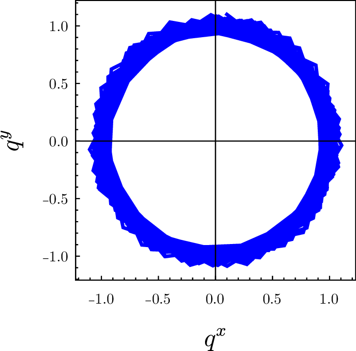
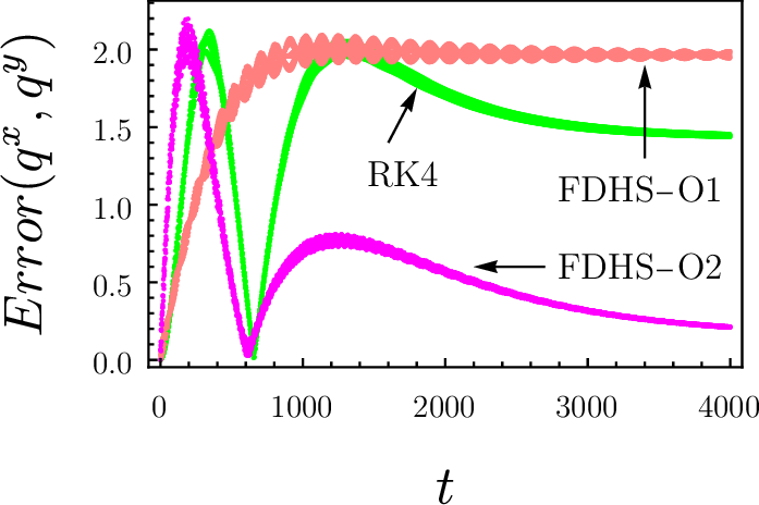
Figure 1: Position evolution (Benchmark and numerical). Parameters: \(\mu=10^{-3}\) and \(h=0.2\). Initial conditions: \(q_0=(0.1,1.1)\),
\(p_0=(0.6,0.1)\). Methods: Benchmark (Blue), FDHS-O1 (Pink), FDHS-O2 (Magenta) and RK4 (Green)..
As this is a forced system, with a friction-type force, it is interesting to compare the energy evolution under the different numerical integrators. Figure 2 (a) shows the (benchmark) evolution of the energy of
the system. Figure 2 (b) compares the errors of the energy estimates for FDHS-O1, FDHS-O2 and RK4. Notice that, qualitatively speaking, all three integrators follow the
benchmark, that is, the error is decreasing; the graph also shows the typical “oscillatory” behavior of the error for the variational integrators. Last, observe how, even the order \(1\) FDHS-O1 outperforms
RK4 in this case.
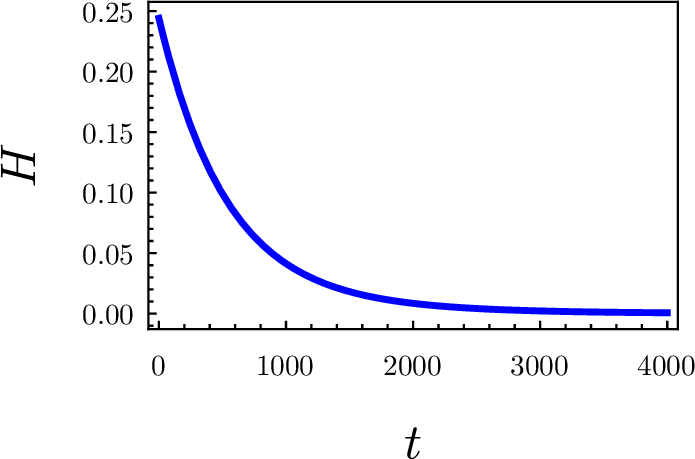
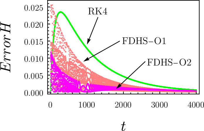
Figure 2: Energy evolution (Benchmark and numerical). Parameters: \(\mu=10^{-3}\) and \(h=0.2\). Initial conditions: \(q_0=(0.1,1.1)\), \(p_0=(0.6,0.1)\). Methods: Benchmark (Blue), FDHS-O1 (Pink), FDHS-O2 (Magenta) and RK4 (Green)..
Acknowledgments↩︎
This document is the result of research partially supported by grants from the Universidad Nacional de Cuyo [code 06/80020240100069UN], Universidad Nacional de La Plata [code SX007], and CONICET.
References↩︎
arXiv:2103.11060“Error analysis of forced discrete
mechanical systems,” J.Geom. Mech., vol. 13, 2021, doi: 10.3934/jgm.2021017.