Post-Generation Curation of Synthetic Images via Homogeneous-Heterogeneous Splitting
July 02, 2026
Abstract
Recent generative models can produce high-quality synthetic images, offering scalable training training data for data-hungry models. Existing approaches to exploiting this potential typically involve 1) training or fine-tuning generators, or 2) using lightweight post-hoc adaptation like prompt engineering or inference-time guidance, making them generator-specific and expertise-intensive. We study a complementary question: given a fixed pool of generated images, can downstream utility be improved purely by selecting an informative subset? The answer is yes. We show that effective selection must counter a structural bias of modern generators: they tend to over-produce canonical modes of each class while under-representing intra-class variation. Building on this insight, we split each real class into a canonical Homogeneous () subset and a non-redundant Heterogeneous () subset, then score synthetic images by a fidelity-diversity criterion that rewards semantic alignment while penalizing canonical redundancy. The method is generator-agnostic and requires no retraining. Across multiple benchmarks, it consistently outperforms state-of-the-art data selection baselines and matches the real-data performance with up to \(40\%\) fewer synthetic samples. The same criterion remains effective when applied on top of stronger task-tuned generators, with gains on both classification and segmentation tasks. Post-generation selection is therefore not a substitute for better generators, but a complementary mechanism for improving the utility of synthetic data.
1 Introduction↩︎
Generative models (GMs) produce high-quality synthetic data and offer a promising solution for data scarcity in data-intensive AI. Recent studies demonstrate that GMs can effectively replicate datasets (CIFAR-10, ImageNet) and improve downstream models trained on such synthetic data in generalization, transferability, and in-domain accuracy [1]–[6].
However, practical challenges remain: 1) synthetic datasets may contain low-fidelity or mislabeled samples, introducing harmful noise; 2) Inadvertently over-representing dominant patterns could transfer inherent biases to downstream models; 3) While scaling the data alleviates these issues, it incurs higher computational overhead and longer training times.
To harness synthetic data, researchers are prioritizing improved generation techniques that yield more faithful and diverse data. These approaches can be broadly categorized into: 1) training- or fine-tuning-based methods [3], [7], which adapt generators to better match target distributions; 2) lightweight strategies like guidance [8]–[12] or prompting [13]–[15]. While effective, these approaches face distinct trade-offs: training-based methods incur substantial computational overhead due to the optimization of large-scale models, whereas lightweight strategies often rely on model-specific configurations, significant domain expertise, or extensive empirical tuning. Alternatively, data selection [16], [17] separates quality control from the image generation, bypassing the typical pitfalls of steering-based methods. This data-centric focus serves as a practical and complementary refinement stage, ensuring high-quality synthetic outputs even after specialized, task-guided generation phases.
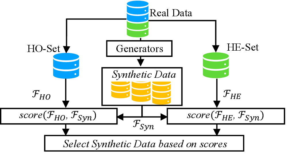
Aligning curated data with the target distribution is a promising post-processing principle. Image–Label Alignment methods [4], [18], [19] assume that high-quality data align strictly with the generative labels, employing pre-trained discriminators to filter out noisy samples; Image–Image Alignment [20], [21] prioritizes synthetic samples that closely resemble real images. Both strategies emphasize fidelity, but largely neglect diversity, reducing the utility of synthetic data [6] due to repeated patterns and missing novel information.
Motivated by these limitations, we propose a fidelity–diversity balanced post-generation curation framework to enhance the utility of synthetic imagery for downstream tasks. In the curation pipeline, we first split the real dataset into two subsets: a Homogeneous set characterized by high internal similarity, and a Heterogeneous set enriched with variation. Based on this partitioning, we design a scoring mechanism to identify and select desired synthetic instances, balancing high semantic quality with representational diversity, shown as Fig. 1). Concretely, we compute two complementary metrics: 1) fidelity scores, measuring semantic similarity to real samples; 2) diversity scores, quantifying the deviation from repetitive patterns. Combining such metrics, we curated the final desired synthetic pool.
To quantify the utility of our curation strategy, experiments are implemented across diverse datasets (e.g., CIFAR-10, ImageNet, etc.) and architectures (e.g., ResNet, ViT). We synthesize data pools using generators trained on target distributions, then apply the curation method to train downstream models for in- and out-of-distribution testings. Furthermore, we apply the curation as a post-process after optimized generations for downstream tasks. Empirical results demonstrate the validity of our post-generation processing under the different settings. In summary, our contributions are as follows:
A nearest-neighbor-cover partition () of real data with a minimality guarantee (Prop. 1), giving an explicit notion of canonical vs.non-redundant samples.
A principled, post-generation selection strategy that jointly quantifies and balances fidelity and diversity. The framework is generator-agnostic, requiring only a synthetic data pool, and avoids costly retraining or fine-tuning of generators.
Extensive experiments validate the approach across classification and segmentation benchmarks with multiple generators and backbones. Our method consistently improves in-domain accuracy and OOD robustness over baselines, plus an additional plug-in evaluation on top of generator-side intervention methods.
2 Related Works↩︎
2.1 Curating Synthetic Data for downstream utility↩︎
Synthetic data has emerged as a promising solution to data scarcity in the AI era [22]–[24]. Recent studies show that models trained on synthetic data can learn robust visual representations [4], [25]–[28]. Moreover, augmenting real datasets with synthetic samples has been shown to further improve model performance [2], [29], [30]. However, the distribution gap between real and synthetic data [6], [31] highlights the need for careful tailoring [5], [24], [32], [33] to fully exploit the potential of synthetic data.
Intervening before or during generation is an effective way to improve the utility of synthetic data. Fine-tuning-based methods adapt generators to target distributions or downstream tasks [3], [7], while prompt-, guidance-, and sampling-based methods steer generated samples toward desired classes, attributes, or harder variations [8]–[10], [14]. Although these approaches can improve the utility of synthetic data, they often require generator access, task-specific tuning, prompt expertise, or additional generation cost. In contrast, post-generation curation offers a practical and scalable alternative to generation-time intervention for improving synthetic data utility.
2.2 Post-Generation Synthetic Data Curations↩︎
Unlike real data pruning [17], [34], [35], synthetic data usage involves generator bias, distribution drift, and mode collapse. Such artifacts require careful curation to steer synthetic pool toward the target.
Fidelity-Guided Curation. High-fidelity generations ensure semantic correctness, making fidelity-based selection effective. Such curation strategies can be broadly categorized into two main approaches: 1) Image-Label
Alignment: pretrained or task-specific models are used to filter low-quality samples by discarding those misclassified within top-\(k\) predictions [36]–[39]. Concretely, CLIP [40] is used to assess image-label semantic alignment [4], [21], [41] ; 2) Image-Image Alignment: this approach quantifies similarity between synthetic and real images to filter out low-quality data that deviate from
the real distribution [20], [21], [42], [43]. Specificly, clustering-based curation [21] use real-data cluster centroids as anchors to retrieve synthetic samples. While straightforward, these methods rely heavily on visual similarity and risk reducing data diversity for downstream tasks.
Diversity-Guided Curations. As generative images become increasingly realistic, diversity is key for downstream usage. Prior works enhance diversity by varying prompts [13], applying text-conditioned augmentation [15], [44], using textual inversion [45], or conditioning on classifier
outputs [46]. While effective, these methods require fine-tuning or prompt
engineering and focus on generation-time diversity, offering little guidance on how to efficiently leverage existing synthetic datasets. Building the priors, we curate synthetic datasets by jointly considering fidelity and diversity, without modifying
generative model output, forming a post-generation data curation pipeline.
3 Methods↩︎
Overview. We target the following post-generation curation problem and assume only sample access to the generator. Given (i) a labeled real reference set \(\mathcal{D}_R=\{(I_i,y_i)\}_{i=1}^{|\mathcal{D}_R|}\), (ii) a synthetic pool \(\mathcal{D}_S=\{\tilde{I}_j\}_{j=1}^{|\mathcal{D}_S|}\) with class assignments inherited from the generator’s conditioning, and (iii) a selection budget \(k\) (possibly much larger than \(|\mathcal{D}_R|\)), the goal is to select \(\mathcal{A}\subseteq\mathcal{D}_S\) so that the selected synthetic training set improves downstream classification on the real distribution.
Our method has two steps. First, we split the real reference images into a Homogeneous subset \(\mathcal{I}_{HO}\) of local representatives and a Heterogeneous subset \(\mathcal{I}_{HE}\) of non-redundant variation (Sec. 3.1). Second, we allocate the synthetic budget across these two subsets and score each synthetic candidate with a partition-conditioned fidelity–diversity criterion (Sec. 3.2). The key design principle is that the selected set should match both the canonical component and the heterogeneous component of the real class, instead of ranking all synthetic images against a single pooled reference distribution.
3.1 Categorizing Homogeneous () and Heterogeneous () Samples↩︎
To guide the selection of synthetic data, we first categorize target real distribution into two distinct sets: Homogeneous () and Heterogeneous (). instances represent the canonical semantics, exhibiting high intra-class similarity in feature space. instances capture greater variation, including less typical instances that contribute to diversity.
Identifying and Instances. We construct the /split from the directed \(1\)-nearest-neighbor (1-NN) graph of each real class in feature space. The construction is local, non-parametric, and costs \(O(n^2d)\) for a class with \(n\) examples and \(d\) is the feature dimension of input. Unlike a centroid-near/far split (\(k\)-means, core-set partitions), it does not impose a global axis through the class: \(\mathcal{I_{HO}}\) contains examples that other examples use as their closest local representatives, while \(\mathcal{I_{HE}}\) contains examples with zero in-degree in this local graph.
Given images \(\mathcal{I}=\{I_1,\ldots,I_n\}\), we extracted \(\ell_2\)-normalized features \(\mathcal{F}=\{f_1,\ldots,f_n\}\) using a pretrained encoder (MoCo v3 [47]). We use cosine distance \(d(f_i,f_j)=1-\langle f_i,f_j\rangle\) throughout. For each \(I_i\), we define its within-class nearest neighbor \[j^\ast(i)=\arg\max_{j\neq i}\langle f_i,f_j\rangle . \label{eq:nn-map}\tag{1}\] Therefore, the set is the image of this map and the set is its complement: \[\mathcal{I_{HO}}=\{I_i:\exists j\neq i,\;j^\ast(j)=i\},\qquad \mathcal{I_{HE}}=\mathcal{I}\setminus\mathcal{I_{HO}}. \label{eq:ho-he}\tag{2}\] Equivalently, in the directed 1-NN graph with edges \(I_i\to I_{j^\ast(i)}\), \(\mathcal{I_{HO}}\) is the set of nodes with positive in-degree and \(\mathcal{I_{HE}}\) is the set of zero in-degree nodes.
Proposition 1 (\(\mathcal{I}_{HO}\) as a minimal nearest-neighbor cover). Assume every sample has a unique within-class nearest neighbor. Then \(\mathcal{I}_{HO}\) is the unique inclusion-minimal subset \(A \subseteq \mathcal{I}\) such that \[\min_{I_i \in A,\, i \neq j} d(f_j,f_i) \;=\; \min_{I_i \in \mathcal{I},\, i \neq j} d(f_j,f_i), \quad \forall\, I_j \in \mathcal{I}. \label{eq:nn-cover-main}\qquad{(1)}\] Thus, with \(\varepsilon = \max_j d(f_j,f_{j^\ast(j)})\), every real sample has an \(\mathcal{I}_{HO}\) representative within distance \(\varepsilon\).
Proposition 1 formalizes the representative role of \(\mathcal{I_{HO}}\): replacing the full class by \(\mathcal{I_{HO}}\) preserves the nearest-neighbor reconstruction cost of every training image. The complement \(\mathcal{I_{HE}}\) should therefore not be read as noise or outliers. It is the part of the class that is not needed as a nearest-neighbor representative for other examples, and is precisely where non-redundant variation can be lost when a generator over-produces canonical images.
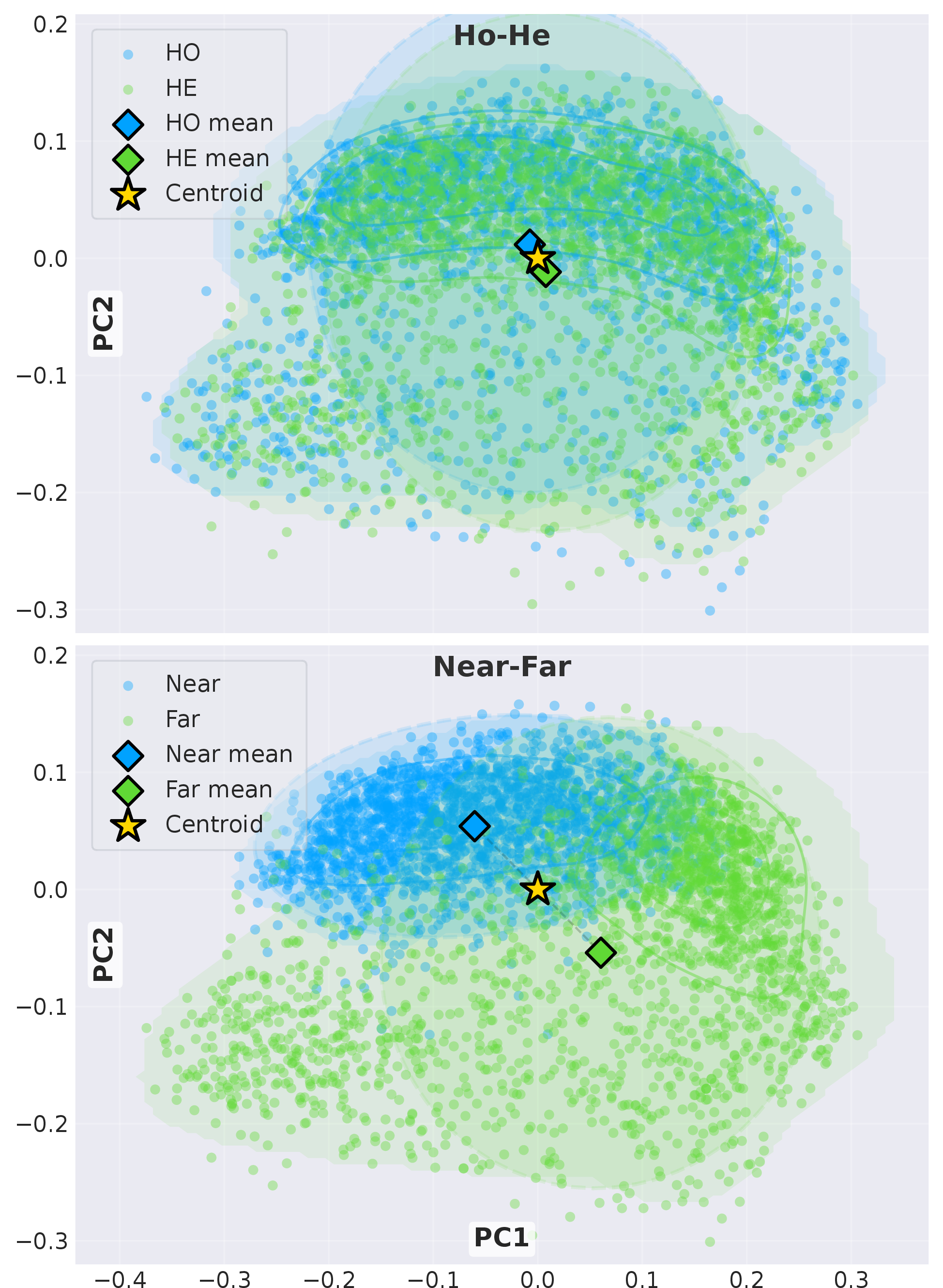
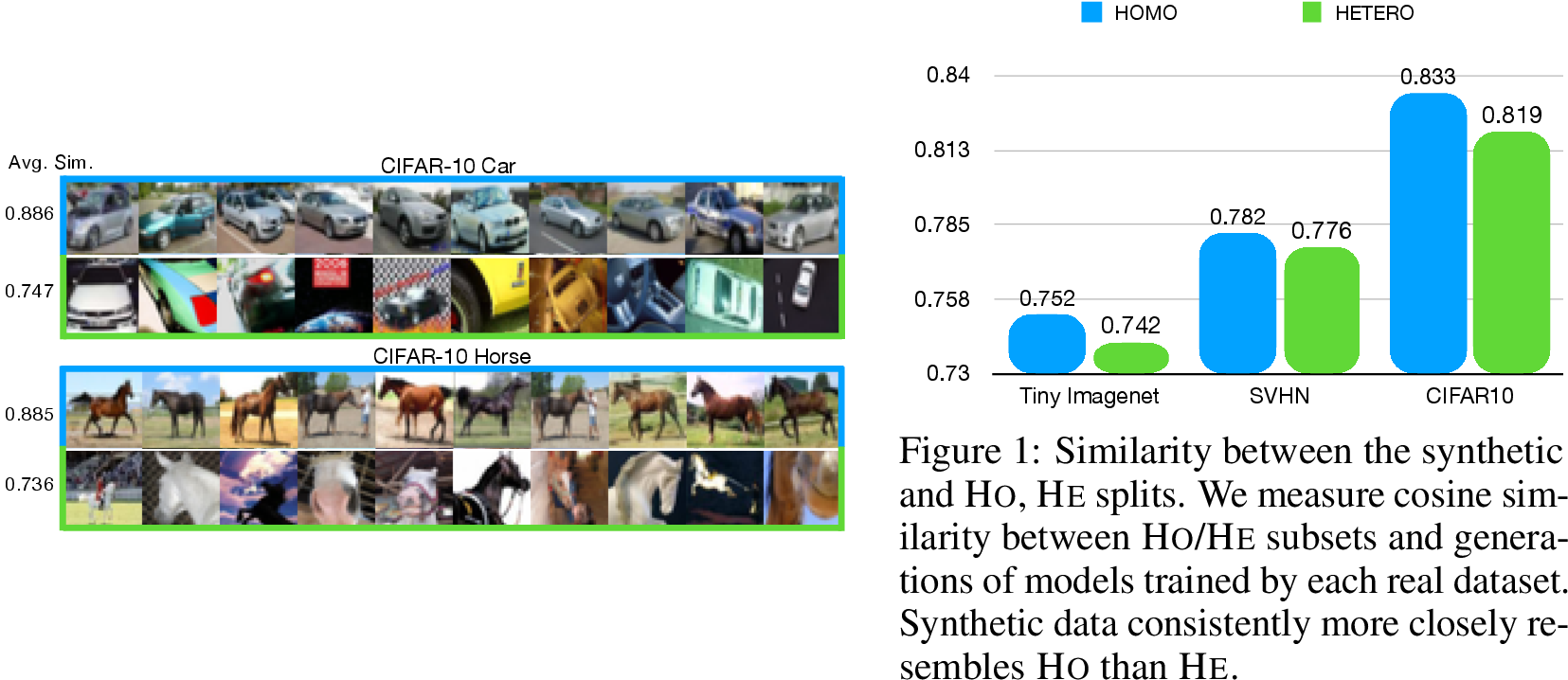
Empirical \(\boldsymbol{\mathcal{I_{HO}}} - \boldsymbol{\mathcal{I_{HE}}}\) Analysis and Impact. As visualized in Fig. 2, the split preserves local neighborhood and keeps each semantic mode mixed across both subsets, avoiding mode imbalance during guided selection. In contrast, centroid-based alternatives that define near/far canonical patterns tend to isolate individual mode regions, yielding suboptimal selection references. Without a complete semantic landscape, prioritizing any single mode during synthetic data curation inevitably overlooks parts of the real distribution, leading to information loss. We also show -partition instances in CIFAR-10 (Fig. [fig:ho95he95samples]). Because samples are retrieved as local representatives, they have higher intra-class similarity than samples, both visually and quantitatively (more cases in Appendix Fig. 10 and Tab. [tbl:tab:ho95he95intr95class]).
Although both \(\mathcal{I}_{HO}\) and \(\mathcal{I}_{HE}\) encompass all distribution modes, we observe an interesting divergence in downstream behaviors: 1) GMs preferentially learn and reproduce \(\boldsymbol{\mathcal{I}_{HO}}\). As quantified in Fig. [fig:ho95vs95he], synthetic data disproportionately mirrors \(\mathcal{I}_{HO}\) over \(\mathcal{I}_{HE}\). This inherent preference indicates that GMs gravitate toward repeated canonical patterns within \(\mathcal{I}_{HO}\), which may explain the persistent diversity limitations observed in modern generative models. 2) Discriminators exhibit a similar performance bias, excelling on \(\boldsymbol{\mathcal{I}_{HO}}\) while struggling with \(\boldsymbol{\mathcal{I}_{HE}}\). This discrepancy indicates that, despite sharing underlying semantics, \(\mathcal{I}_{HE}\) contains inherently more challenging cases that discriminators fail to model effectively (empirical supports across datasets is provided in the Appendix [discriminators], Fig. 13).
3.2 Synthetic Data Selection Strategy↩︎
Given the and sets, we propose a synthetic data selection strategy to identify desirable instances from a fixed synthetic pool. The core objective is to ensure high semantic fidelity while enhancing diversity by prioritizing samples that diverge from the dominant patterns in .
Partitioned Selection Strategy. Unlike prior methods that treat the entire real dataset as a single reference for data selection, we propose a partitioned selection approach. We treat and as separate partitions and select synthetic instances by referring to real images within each partition under the same principle: desired synthetics should be sufficiently close to their corresponding real instances, while prioritizing those that deviate from canonical representations. By combining the selection results from and instances, we obtain the final selected pool.
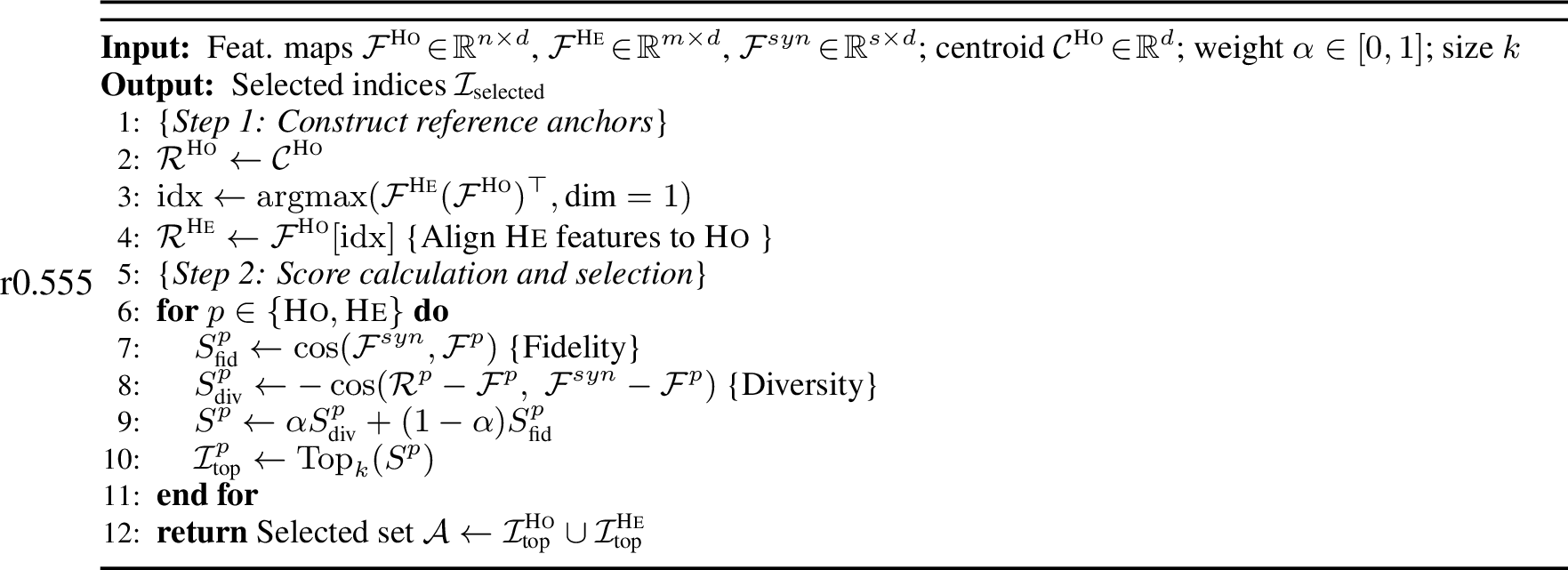
Concretely, we compute a selection score \(S^p\) for each synthetic sample based on its correlation with partition \(p\in\{\ho, \he\}\). Samples are ranked within each partition, and the instances with high \(S^p\) get retrieved. Alg. 4 for the pseudo‑code of our selection procedure.
Scoring Mechanism for Each Partition. Our selection mechanism balances two competing objectives: the fidelity score, measuring how closely a synthetic instance resembles the real, and the diversity score, measuring how much it deviates from canonical patterns in the real dataset.
1) Fidelity Score. The fidelity score \(S^p_{\text{fid}}\) quantifies how well the synthetic samples align with the real distribution of partition \(p\). We measure this using the cosine similarity between the synthetic features \(\mathcal{F}^{syn}\) and the real features \(\mathcal{F}^p\), as defined in Eq. 3 . A higher fidelity score indicates that the synthetic samples closely resemble the real data in the corresponding partition: \[S^{p}_{\text{fid}} = \cos(\mathcal{F}^{syn}, \mathcal{F}^p). \label{eq:fidelity}\tag{3}\]

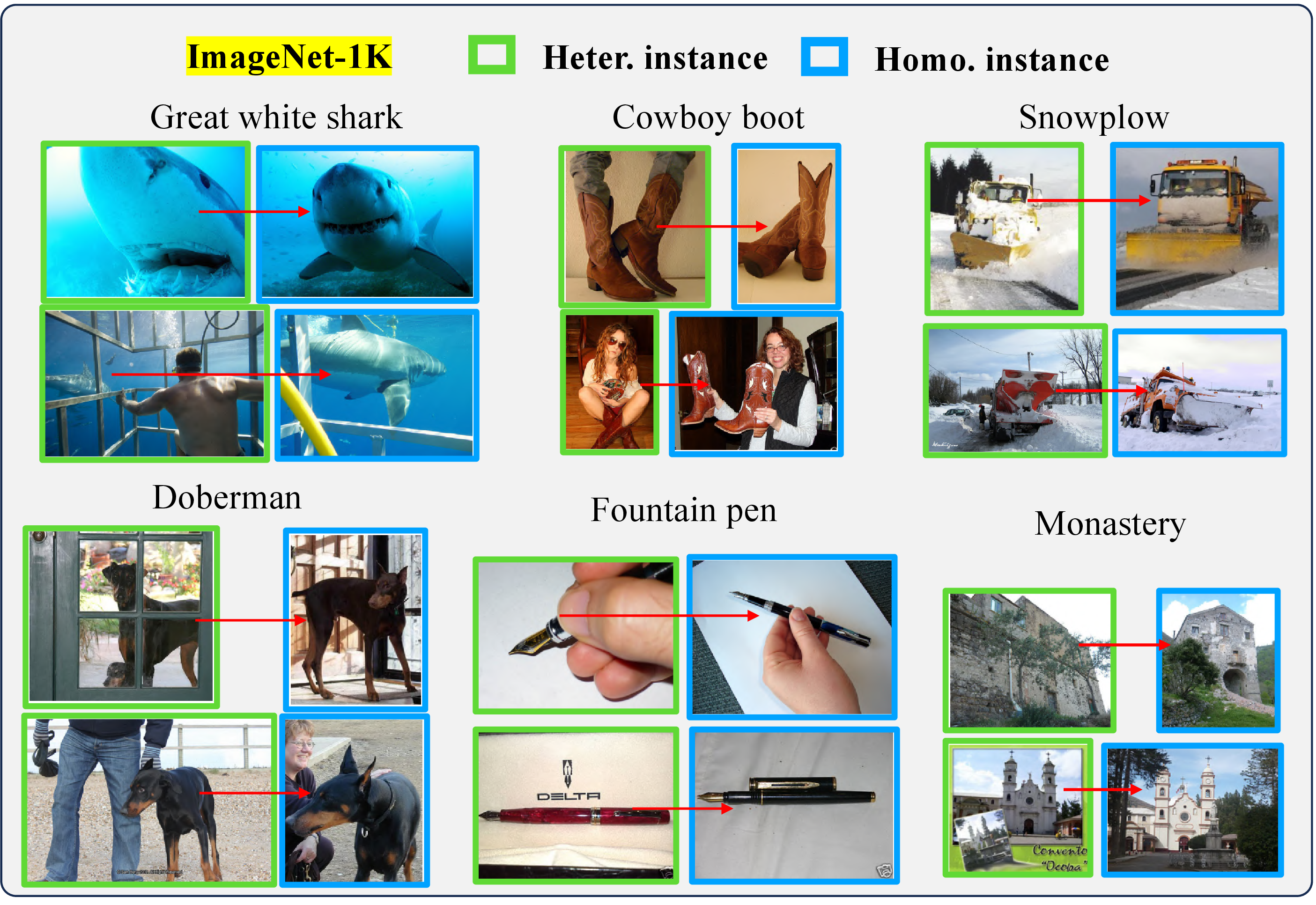
2) Diversity Score. The diversity score \(S^p_{\text{div}}\) is designed to encourage the selected synthetic samples to deviate from canonical patterns. To achieve this, we define a subset-specific reference anchor \(\mathcal{R}^p\). For the subset, the anchor is the centroid of the real features (\(\mathcal{R}^{\ho} = \mathcal{C}^{\ho}\)). For the subset, the anchor is the nearest matching feature in the subset (\(\mathcal{R}^{\he} = \mathcal{F}^{\ho}[\mathrm{idx}]\)). The diversity metric is then formulated as the negative cosine similarity between two directional vectors, as defined in Eq. 4 : one from the real instance \(\mathcal{F}^p\) to the anchor \(\mathcal{R}^p\), and the other from the same real instance to the synthetic data \(\mathcal{F}^{syn}\) (representative visual cases are shown in Fig. 14 of the Appendix). \[S^{p}_{\text{div}} = -\cos(\mathcal{R}^p - \mathcal{F}^p, \; \mathcal{F}^{syn} - \mathcal{F}^p). \label{eq:diversity}\tag{4}\] As illustrated in Fig. 5, if these two vectors point in opposite directions, the cosine similarity is negative, leading to a higher diversity score. If the vectors are aligned, the synthetic sample is closer to the homogeneous distribution, resulting in a lower diversity score.
3) Total Score. To control the trade-off between fidelity and diversity, we define the score as: \[{S}^p = \alpha \cdot S_\text{div}^p + (1 - \alpha) \cdot S^p_\text{fid}, \label{f:core95score}\tag{5}\] where \(\alpha\) is a hyperparameter that determines the selection priority. \(\alpha = 0\) (MaxSim) prioritizes fidelity, ensuring that synthetic instances closely resemble real ones. \(\alpha = 1\) (MaxDiv) prioritizes diversity, encouraging synthetic samples that deviate from the dominant patterns of real data. Adjusting \(\alpha\) enables flexible control over the selection behavior to match downstream needs.
Practical Considerations. (a) Complexity. Building the 1-NN graph costs \(O(n^2d)\) after feature extraction, where \(n\) is number of real samples, \(d\) is feature dimension. Scoring is implemented as batched matrix multiplication and costs \(O(|\mathcal{D}_S|nd)\), where \(|\mathcal{D}_S|\) denotes the number of synthetic candidates. (b) Encoder choice. The split is relative to encoder \(\phi\), so a domain-mismatched encoder can degrade curation. Sec. 5 compares representative encoders and shows that the gains are not tied to a single feature extractor. (c) No balanced requirement. The split is induced by the 1-NN graph; it does not assume a target ratio or require pre-labeled canonical examples. Unequal partition sizes only change how the synthetic budget is allocated across the two scoring branches: larger partitions receive proportionally more selections, while smaller partitions still receive explicit coverage. Thus, the near-balanced masses observed in the experiments are an empirical property of the datasets, not a requirement of the method.
4 Experiments↩︎
We evaluate post-generation curation under two settings. The general setting fixes a generator and a synthetic pool, applies each selection method under the same budget, and trains downstream classifiers for in-domain (Sec. [sec:scaling]) and out-of-domain (OOD) (Sec. 4.3) evaluation. The plug-in setting (Sec. 4.4) applies the same curation step after task-customized generation to test whether selection remains useful when the generator has already been adapted to a downstream task.
4.1 Datasets and Baselines↩︎
Datasets. The main evaluation spans classification and segmentation datasets with increasing scale and visual complexity. For SVHN [48],
CIFAR-10 [49], and Tiny-ImageNet [50], covering 10, 10, and 200 classes respectively, we curate synthetic pools generated by EDM [51]. For
large-scale validation, we use ImageNet-1K (IN-1K) synthetics generated by EDM2 [52], [53]. In total, the evaluation covers 4 in-domain benchmarks and 9 OOD benchmarks. The plug-in experiments further use task-customized generation for ImageNet-100 (IN-100) [54] and VOCaug [55] (Sec. 4.4).
Baselines. For each comparison, all selection methods operate on the same synthetic pool and use the same selection budget. In the main evaluation, we compare three categories of selection methods. RandSelect [56]–[58] is an uninformed random baseline.
CLIP-Align [4] represents image–label alignment by ranking generated images with CLIP
text–image scores. RealScore [20] and SBSim [21] represent image–image alignment. In the plug-in setting, the baselines are generation-side interventions that already target the downstream task: inference-time intervention [59] and the fine-tuned generator JoDiffusion [60].
Implementation. Unless otherwise stated, we use \(\alpha=0.5\) for all main experiments and keep the downstream training recipe fixed within each comparison.
4.2 Scaling Model Performance with Selective Synthetic Data↩︎
We first ask whether curation improves the value of synthetic data as the training budget grows. For each selected set, we train the same downstream architecture with the same recipe and evaluate on the corresponding real test set. The small- and medium-scale experiments use ResNet-18/50 [61] and EfficientNet-B0 [62]; the IN-1K experiments further include ViT-B/16 [63]. Full training details are provided in Appendix 11.2.
| Selection | Scratch | Fine-tune | ||||||||
| +0 | +1M | +3M | + 0 | +1M | +3M | 1M | 3M | 1M | 3M | |
| Random | 64.22 | 70.90 | 73.54 | 69.27 | 72.03 | 72.13 | 78.52 | 78.68 | 71.90 | 73.65 |
| RealScore | - | 70.92 | 73.53 | - | 72.01 | 72.16 | 78.52 | 78.67 | 71.93 | 73.62 |
| CLIP-Align | - | 69.18 | 70.88 | - | 69.44 | 70.98 | 72.40 | 75.23 | 62.57 | 67.57 |
| SBSim (\(\alpha=0\)) | - | 70.95 | 73.23 | - | 71.97 | 72.18 | 78.58 | 78.76 | 72.18 | 74.14 |
| Diversity (\(\alpha=1\)) | - | 71.42 | 73.79 | - | 71.80 | 73.25 | 78.72 | 79.14 | 72.25 | 74.25 |
| Ours | - | 71.49 | 74.02 | - | 72.09 | 73.33 | 78.97 | 79.36 | 73.14 | 74.76 |
4.5pt
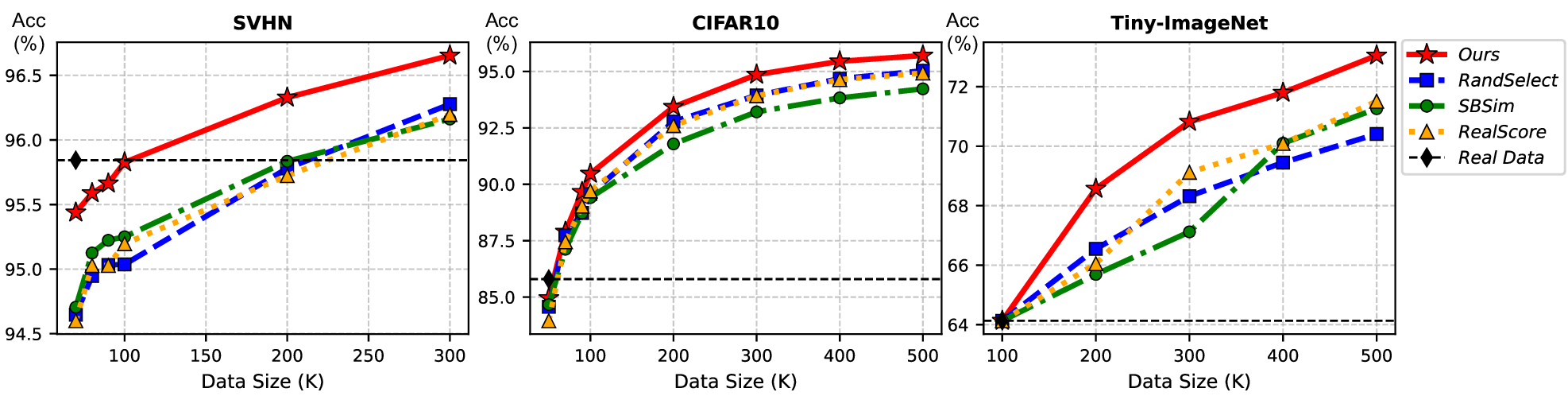
Across SVHN, CIFAR-10, and Tiny-ImageNet, Fig. 6 shows consistent gains from our curation, with the largest benefits appearing as the selection budget grows. On
SVHN, our method matches the real-data baseline with substantially fewer examples ( k synthetic samples), whereas alternative methods require over 200 k to reach comparable accuracy. On CIFAR-10, our method achieves 95%
accuracy with 300 k samples, while RandSelect and RealScore require around 500 k, and SBSim demands substantially more. This pattern is consistent with the failure mode targeted by our method: once high-fidelity canonical samples
saturate, additional gains depend on selecting less redundant variation. For the harder Tiny-ImageNet, we use selected synthetic data as augmentation since synthetic-only training suffers a larger domain gap; our curation improves
ResNet-50 accuracy at every augmentation budget.
For IN-1K, prior work [2], [3], [6] reported a persistent gap between real and synthetic data at ImageNet scale. We therefore
evaluate two practical uses of selected synthetic data: 1) training models from scratch with synthetic data as augmentation and 2) fine-tuning pre-trained models using synthetic data alone. Tab. 1 reports results for
ViT-B/16 and ResNet-50 with 1M and 3M selected images from an EDM2 pool. Using the same training configuration, our method gives the best accuracy across all settings, indicating that the fidelity–diversity balance remains useful at ImageNet scale.
4.3 Enhancing Model Generalizability with Selected Samples↩︎
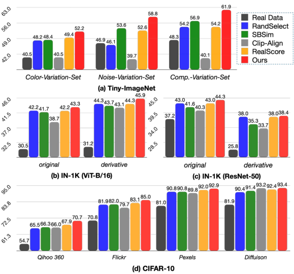
Models trained on informative and diverse data are expected to achieve greater robustness under OOD settings. In this part, we evaluate the generalizability of the best models trained (from scratch) in the previous section with OOD datasets. The results demonstrate that curated synthetic data improves model generalizability.
OOD of Tiny-ImageNet. We use Tiny-ImageNet-C [64], which incorporates various types of corruption. We classify them into three types: color-variation set (brightness adjustment, contrast variation), noise-variation set (pixelation, Gaussian noise, motion blur), and compression-variation set (JPEG compression). The results are reported in Fig. 7 (a). OOD of IN-1K. We use several OOD datasets and categorize them into two groups 1) original suite, including ImageNet-V2 [65] and ImageNet-Sketch [66]; 2) derivative suite, including ImageNet-C [67], -Drawing, and -Cartoon [68], derived from the validation set (Appendix [in-1k-ood] for details). The evaluation results are summarized in Fig. 7 (b), (c). OOD of CIFAR-10. CIFAR-10-Warehouse [69] is used as a benchmark, collecting data from diverse sources (different search engines). The results are reported in Fig. 7 (d). More results (OOD of SVHN, examples of OOD data) are presented in Appendix 11.4.
4.4 Plug-in Curation after Generator-Side Interventions↩︎
We next test whether curation remains useful after the synthetic pool has already been improved by a generator-side intervention. Keeping each task-adapted pool fixed, we apply our selection as a plug-in post-processing step. We study two representative intervention types: inference-time generator intervention for classification [59] and generator fine-tuning for segmentation [60].
r0.42
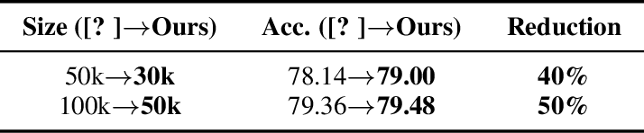
Classification. We apply our curation to synthetic images generated with inference-time intervention [59] on IN-100, then train ResNet-18 on the selected data. As shown in Tab. ¿tbl:tab:data95reduction?, our curation further improves synthetic data utility: curation provides both an equal-budget gain and a 40–50% data reduction on task-aware samples.
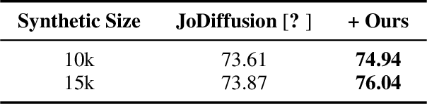
Segmentation. We curate synthetic VOCaug data produced by the fine-tuned generator JoDiffusion [60], then train the downstream segmentation model (DeepLabV3 [70]). In Tab. [tbl:tab:data95size95comparison95in95segmentation], we report mIoU, showing that our method provides additional gains on top of customized generation via fine-tuning. Overall, both results suggest that post-generation curation is a generator-agnostic approach that further improves the utility of optimized synthetic data, highlighting the practical value of our curation strategy.
5 Analysis and Discussion↩︎


Figure 8: Testing accuracy versus trade-off \(\alpha\) (0 = fidelity, 1 = diversity). Each subfigure compares the 100K, 300K, and 500K settings with trend lines, and the optimal point on each curve is marked
by a star. Results are reported with ResNet-18 using the average accuracy over 8 runs.. b — StyleGAN [71]
(FID: 3.17), c — EDM [72]
(FID: 2.67), d — EDM2 [52]
(FID: 1.39)
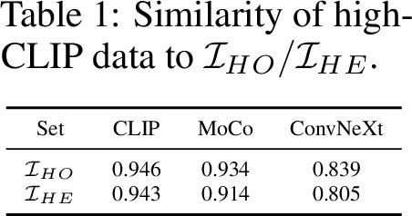
CLIP Filtering Biases Toward Canonical Modes. The weak performance of CLIP-Align in Sec. 4.2 suggests that image–text alignment alone is not a sufficient selection criterion. Tab. ¿tbl:tab:feature95similarity? provides a quantitative diagnostic on CIFAR-10: High-CLIP-score samples are consistently closer to \(\mathcal{I}_{HO}\) than to \(\mathcal{I}_{HE}\) across CLIP, MoCo, and ConvNeXt features. This supports the interpretation that CLIP filtering over-selects canonical modes and under-covers harder variations.
Generator Quality and Data Budget Shift the Optimal Fidelity-Diversity Balance (\(\boldsymbol{\alpha}\)). We explore the relationship between \(\alpha\) in Eq. 5 and different GMs. Our experiments use 1M synthetic CIFAR-10 samples from three GMs. As shown in Fig. 8, the optimal \(\alpha\) depends on both the quality of the synthetic data and the volume of training data. (1) For StyleGAN2 (Fig. 8 (b)), which yields the highest FID, fidelity remains the key factor for classification performance; (2) When the generated distributions are closer to the real (as in EDM and EDM2), Figs.8 (c), 8 (d) demonstrate the benefit of tuning the trade-off factor \(\alpha\). (3) Arcoss all the datasets, as the training volume increases, the optimal \(\alpha\) shifts toward larger values, underscoring the increasing importance of diversity at larger scales, where canonical high-fidelity samples provide limited additional gains. (4) In terms of the best \(\alpha\) in each GMs, the biggest shift is observed in the most advanced EDM2, suggesting that with larger training volumes and highly realistic generations, diversity becomes the decisive factor.
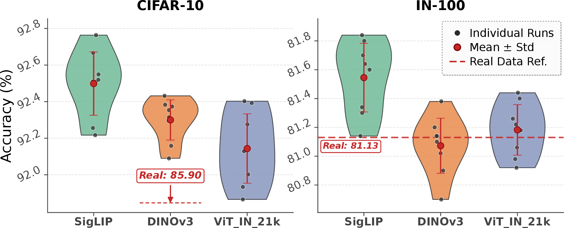
Impact of Feature Extractors. Since our strategy relies on image features, we examine whether the choice of feature extractor matters. We conduct an ablation study using three representative encoders, each reflecting a distinct training
paradigm: SigLIP (text–image alignment) [73], DINOv3 (self-supervised) [74], and ViT (supervised). Evaluations are performed on two datasets with different image resolutions, CIFAR-10 and ImageNet-100 (configurations are summarized in Appendix 12.2). The results, summarized in Fig. 9, show that although SigLIP achieves the best performance, the absolute differences among extractors remain modest. This suggests that
SigLIP is a promising choice, but its impact is relatively minor compared to the quality of synthetic data and the choice of \(\alpha\) in the proposed strategy.
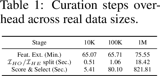
Curation Overhead Is Small Relative to Training. Comparing to previous post-generation selection, our curation introduces unique cost in \(\mathcal{I}_{HO}/\mathcal{I}_{HE}\) splitting, scoring and
selection. Once features are extracted, all such operations reduce to batched cosine similarity computations that are GPU-friendly and fast in practice (implementation in Appendix [Code:32scoring], 13.2). Tab. [tbl:tab:runtime95scale] shows the runtime of
each stage of our curation for 10M synthetic samples across varying real-data scales. Feature extraction dominates the overall overhead. Since it is a one-time inference cost shared by most instance-selection baselines, the overhead specific to our method
remains negligible even at large scales.
3pt
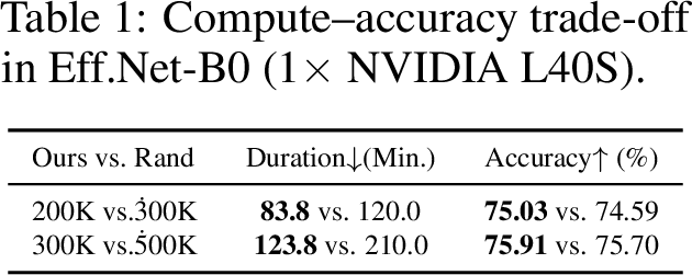
Furthermore, when downstream training is considered, the extra curation cost is well justified. In the Tiny-ImageNet setting, curation of a 1M-image pool takes 3.8 minutes in total (3.5 minutes for feature extraction and 0.3 minutes for scoring and selection). In contrast, training on 200K, 300K, and 500K augmented samples takes 80, 120, and 210 minutes, respectively. As shown in Tab .[tbl:tab:compute95compare], despite incurring 3.8 additional minutes over random selection, our method delivers better performance with fewer training samples, effectively compensating for the curation overhead in downstream training.
The Characteristics of Split in Real Data. Splitting \(\mathcal{I_{HO}}\) and \(\mathcal{I_{HE}}\) within a class across datasets, the number of samples in each subset remains nearly equal, suggesting that approximately half of the samples effectively capture the primary semantics of the class. Using \(\mathcal{I_{HO}}\) and \(\mathcal{I_{HE}}\) as curation references, we observed that although the two sets have comparable volumes, \(\mathcal{I_{HO}}\) yields fewer unique synthetic instances. We attribute this to the higher intra-class similarity within \(\mathcal{I_{HO}}\) (Tab. [tbl:tab:ho95he95intr95class] in the Appendix), which makes it more challenging for GMs to capture fine-grained variations among similar concepts, compared to the more diverse \(\mathcal{I_{HE}}\).
6 Conclusions↩︎
We introduced a generator-agnostic framework for post-generation curation of synthetic images. By splitting real data into and references and selecting synthetics with a partition-wise fidelity–diversity score, the method improves in-domain accuracy, strengthens OOD generalization, reduces the amount of synthetic data needed to match real-data baselines, and remains complementary to task-customized generation for both classification and segmentation. The analysis further suggests a practical principle for synthetic-data use: as generator fidelity and training budgets increase, curation should shift from merely retaining recognizable samples toward allocating more budget to non-redundant variation.
Appendix
The supplementary material is organized by the role each section plays in supporting the main paper. Appendix 7 first gives visual examples and intra-class statistics that characterize the /partition. Appendix [app:hohe-theory] explains the motivation and theoretical interpretation of the partition. Appendix [discriminators] examines how the /split exposes generator and discriminator biases. Appendix [app:selection-details] describes the synthetic-data selection procedure and visualizes the diversity score. Appendix 11 provides the full experimental details, including compute resources, generator usage, training recipes, in-domain results, and out-of-domain results. Appendix 12 reports additional ablations, Appendix [Code:32implement] gives the scoring and selection implementation, and Appendices 14–15 discuss limitations and broader impacts.
7 Visual and Statistical Properties of the HO/HE Partition↩︎
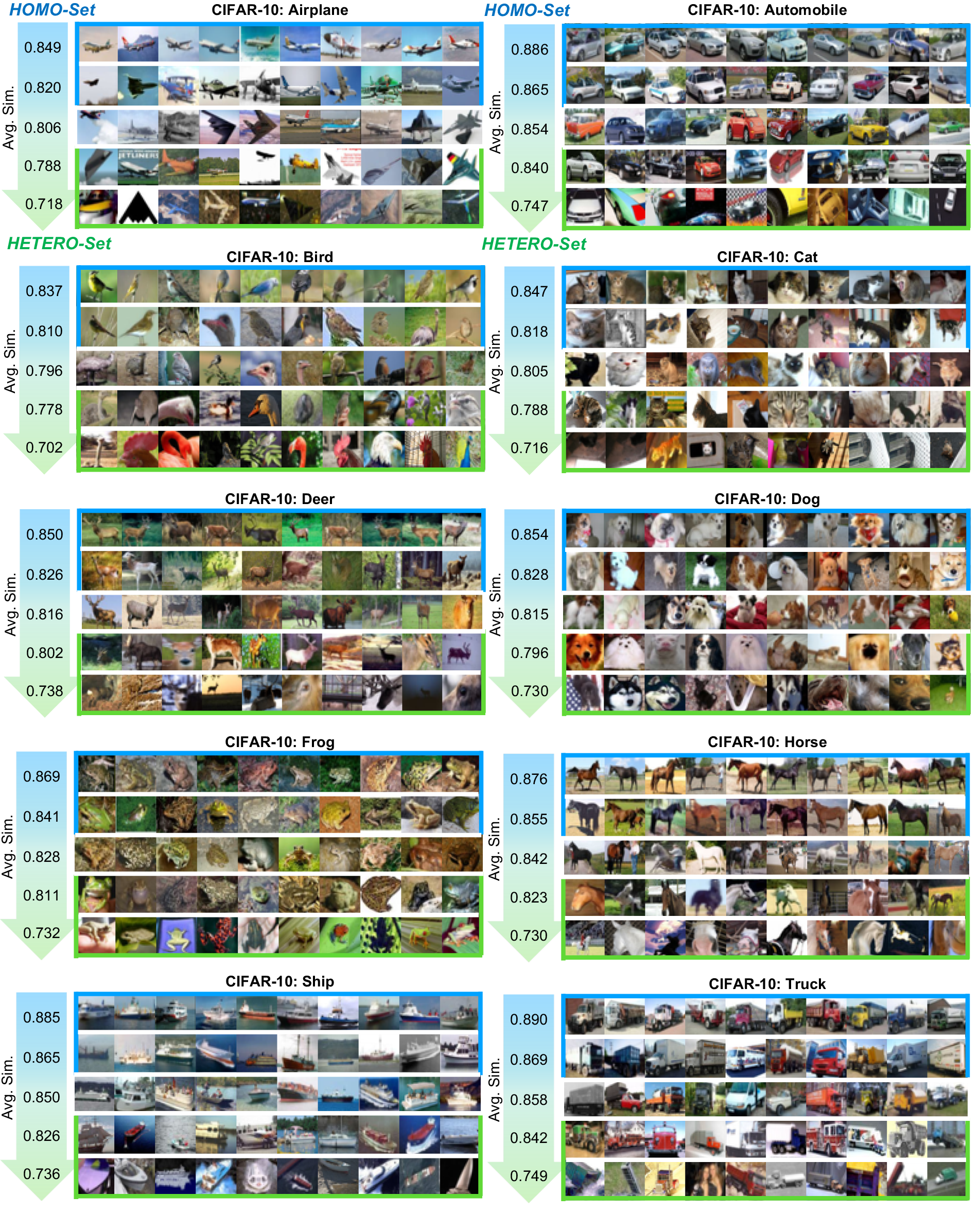
This section provides the visual and quantitative evidence referenced in Sec. 3.1. We partition each real class into \(\mathcal{I}_{HO}\), which contains local canonical representatives, and \(\mathcal{I}_{HE}\), which contains less redundant intra-class variation. Fig. 10 shows CIFAR-10 examples, and Tab. [tbl:tab:ho95he95intr95class] shows that \(\mathcal{I}_{HO}\) has higher intra-class similarity than \(\mathcal{I}_{HE}\) across datasets.
| Subset | SVHN | CIFAR-10 | Tiny-ImageNet | ImageNet-1K |
|---|---|---|---|---|
| \(\mathcal{I}_{HO}\) | 0.8507 | 0.7948 | 0.8236 | 0.8000 |
| \(\mathcal{I}_{HE}\) | 0.8385 | 0.7887 | 0.7894 | 0.7725 |
8 Motivation and Theoretical Justification of -Partition↩︎
In Sec. [main:graph95theory], we argue that the proposed partition admits a theoretical justification under a graph-based view. In this section, we further elaborate the motivation behind the and design and provide a formal analysis showing why optimizing with respect to this partition is well-aligned with the learning objective in our setting.
8.1 Semantic-mode diversity and Variation Diversity↩︎
To clarify the design of our real data partition, we first distinguish between semantic-mode diversity and variation diversity. We provide a PCA visualization in Figure11. In Figure11 (a), the real data are partitioned into two sets based on the distance of each instance to the class centroid: the “near” set contains canonical patterns, while the “far” set consists of patterns that are less similar to the semantic core and therefore exhibit higher semantic-mode diversity. Each of them cover the subregion of original feature space. In contrast, Figure 11 (b) illustrates our /partition, where both and cover all semantic modes present in the real data, and the diversity in manifests as variation diversity, rich variations around each semantic mode across the entire dataset.
Thus, Figure11 (a) illustrates semantic-mode diversity: the “near” and “far” sets are distinguished by the presence of different semantic modes in each subregion. In contrast, Figure11 (b) shows the /partition, where the two sets are distinguished by the variation level within each mode across the entire feature space, rather than by different modes themselves.
8.2 Why we choose -PARTITION↩︎
Standard image augmentations improve model performance by increasing variation within the dataset while preserving the main semantics. Inspired by this, we hypothesize that, when curating synthetic data, if we can construct a set that covers all semantic modes while exhibiting high variation within each mode, we can similarly expect performance gains. Based on this idea, we propose the /partition of the real data, which preserves all modes (as shown in Figure11 (b)) but explicitly distinguishes them by their level of intra-mode variation, and use them as guidance for synthetic data selection.
8.3 Nearest-neighbor representative coverage↩︎
For each real feature \(r_i\), define its nearest neighbor by \[j(i)=\arg\min_{j\neq i} d(r_i,r_j).\] The set is the image of this nearest-neighbor map, \(H=\{r_{j(i)}:i\in[n]\}\), and the set is \(E=R\setminus H\). Equivalently, if we build the directed 1-nearest-neighbor graph by drawing an edge \(r_i\to r_{j(i)}\), then \(H\) is the set of nodes with positive in-degree and \(E\) is the set of zero in-degree nodes.
Proof of Proposition 1. For any \(r_i\), the feature \(r_{j(i)}\) belongs to \(H\) by construction and \(j(i)\neq i\). Therefore \[\min_{h\in H,\,h\neq r_i} d(r_i,h) \leq d(r_i,r_{j(i)}) = \min_{r\in R,\,r\neq r_i} d(r_i,r).\] Since \(H\subseteq R\), the reverse inequality holds automatically, giving equality for \(H\).
Conversely, let \(A\subseteq R\) satisfy the equality in Proposition 1 for every \(r_i\). Under the unique-nearest-neighbor assumption, the only element of \(R\setminus\{r_i\}\) that attains the right-hand side is \(r_{j(i)}\). Hence \(r_{j(i)}\in A\) for all \(i\), and thus \(H\subseteq A\). Since \(H\) itself satisfies the equality, it is the unique inclusion-minimal subset with this property.
Finally, set \(\varepsilon=\max_i d(r_i,r_{j(i)})\). The equality just proved implies \[\min_{h\in H,\,h\neq r_i} d(r_i,h)=d(r_i,r_{j(i)})\leq \varepsilon\] for every \(r_i\in R\), yielding the stated coverage radius. ◻
This result gives the precise sense in which contains canonical representatives: it is the smallest set that preserves every training point’s nearest-neighbor reconstruction cost. The complement is therefore not “noise” or “outliers” by definition; rather, it contains real samples that are not needed as nearest-neighbor representatives for other samples and thus encode less redundant local variation.
8.4 Geometric interpretation of the diversity score.↩︎
The diversity score has a simple angular meaning. For an anchor \(r\), let \(a_r=h(r)-r\) be the direction from \(r\) to its nearest neighbor. If a synthetic candidate \(z\) moves from \(r\) inside a cone of half-angle \(\theta\) around \(a_r\), then \[\left\langle \frac{z-r}{\|z-r\|}, \frac{a_r}{\|a_r\|} \right\rangle \geq \cos\theta \qquad\Rightarrow\qquad S^{\he}_{\mathrm{div}}(z,r)\leq -\cos\theta .\] Thus increasing \(\alpha\) suppresses candidates that are close to an anchor only by drifting back toward the canonical direction. This is the intended complement to the fidelity term: fidelity keeps the selected sample semantically aligned with an anchor, while diversity discourages repeated canonical collapse.
8.5 Graph interpretation of the partition.↩︎
In this section, we discuss the properties of the partition and prove its optimality in our setting. As defined in Eqs. 2 ,, we can review such partitions in the graph setting. In the original dataset, each feature of the image could be viewed as the node, and the cosine similarity between different features could be used as the distance connecting each pair of nodes (higher similarity corresponds to a smaller distance and less cost for transfer). Then we can compose a fully connected graph \(G=(V,E)\), and \(V\) is the set of nodes, and \(|V| = n\), and \(E\) is the set of edges, \(|E| = n\times n\).
To find the “hubs" in the graph, we traverse all nodes in the graph and connect each node to its single nearest neighbor, forming a directed graph \(G'= (V, E')\), where \(|E'| = n\). Under this setting, is equivalent to the collection of nodes whose in-degree is positive.
So in the graph setting, the definition of could be rewritten as:
\[\mathrm{HO} = \left\{ a \in V \;\middle|\;\exists b \in V \setminus \{a\}, \text{ such that } \forall c \in V \setminus \{a, b\}, d(a, b) \le d(c, b) \right\}\]
Based on the definition above, we can derive the following properties:
To reach any node \(b\) in the graph, starting from a node in (different from \(b\)) consistently yields the minimal cost. Such property implies that learning the pattern in , and then we can reconstruct the whole original feature space with the smallest cost.
Suppose, in the original graph, each node has a single nearest neighbor. Then, theoretically, is a minimal subset of nodes such that every node in the graph can be reached from some node in with minimal cost.


Figure 11: PCA visualization in ImageNet-1K (n03769881), using different partition strategies. a — Centroid Partition, b — -Partition
Training downstream models on a given dataset can be interpreted as optimizing the model to capture the full set of patterns in the underlying feature space. From a graph perspective, once the model learns the patterns in , it can often propagate this knowledge to other modes with relatively little additional cost. As a result, after sufficient training, downstream models naturally exhibit a preference for , where the patterns are easier to learn and generalize.
Therefore, motivated by this insight, we propose a synthetic data selection strategy built on the partition to better unlock the value of synthetic samples for downstream training.
9 Generator and Discriminator Biases in the /Split↩︎
Echoing the discussion of Downstream Model Preference in Sec. [preference], \(\mathcal{I}_{HO}\) and \(\mathcal{I}_{HE}\) together constitute a complete real dataset, and when such data are used to train downstream models, these characteristics may be implicitly inherited.
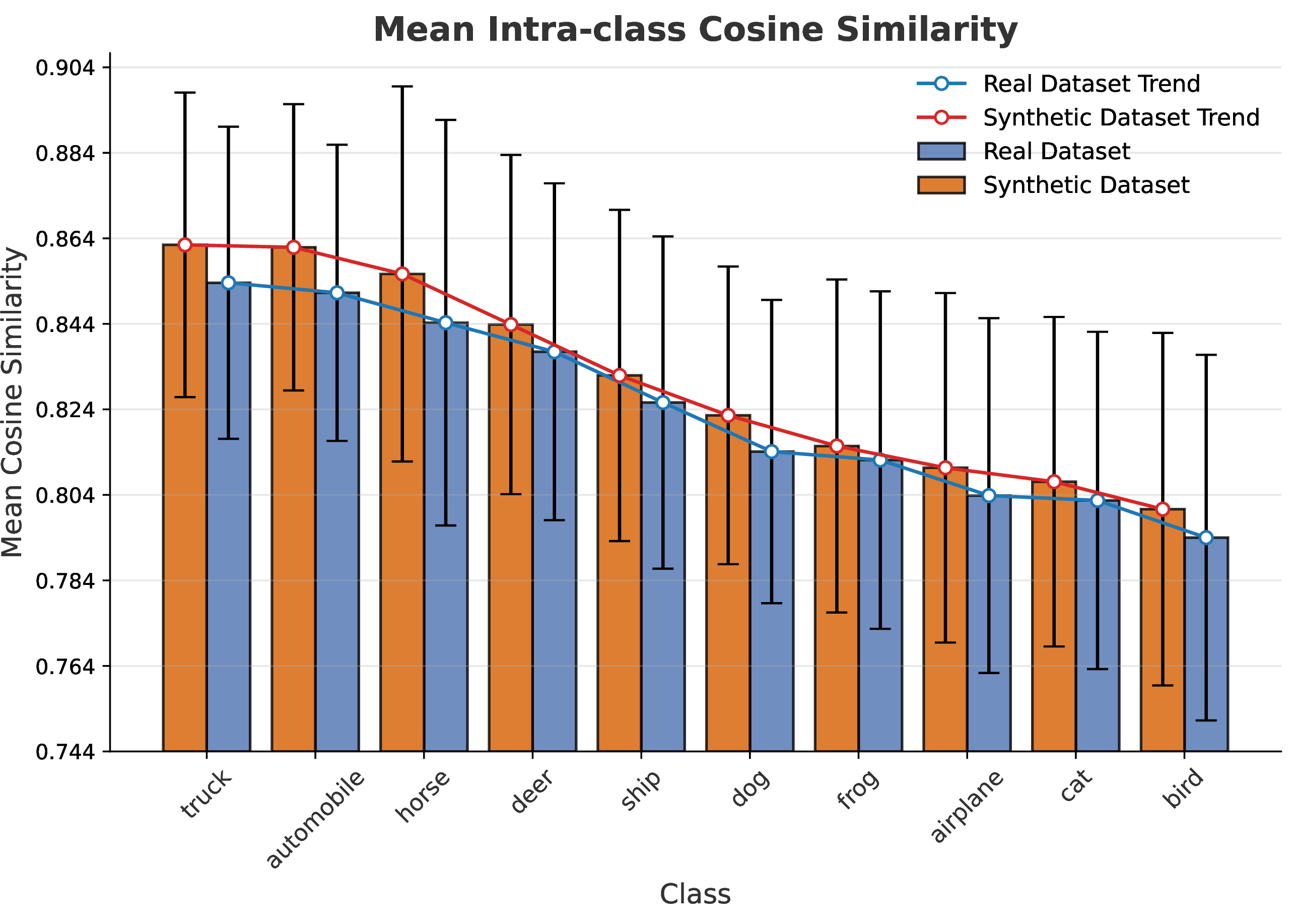
For Generative Models, we investigate the relationship between generated instances and real instances in \(\mathcal{I}_{HO}\) and \(\mathcal{I}_{HE}\). As shown in Figure [fig:ho95vs95he], samples generated by EDM[72] exhibit higher similarity to those in the \(\mathcal{I}_{HO}\), highlighting the well-known limitation of reduced diversity in generative data. Since \(\mathcal{I}_{HO}\) samples capture canonical patterns that are easier for generative models to learn, this bias toward \(\mathcal{I}_{HO}\) leads to higher intra-class similarity compared to real datasets, thereby reducing overall diversity, as shown in Figure 12.
For Discriminators, trained on real data, we observe a clear performance gap between \(\mathcal{I}_{HO}\) and \(\mathcal{I}_{HE}\), even when evaluation is conducted on the original training set. As shown in Figure 13, we run inference using off-the-shelf pretrained models (referring Table 3) on the training datasets and consistently find higher accuracy on \(\mathcal{I}_{HO}\) than on \(\mathcal{I}_{HE}\). We attribute this gap to differences in canonicality: \(\mathcal{I}_{HO}\) contains more canonical instances that are easier for models to fit, whereas \(\mathcal{I}_{HE}\) demands modeling a broader range of intra-class variations.
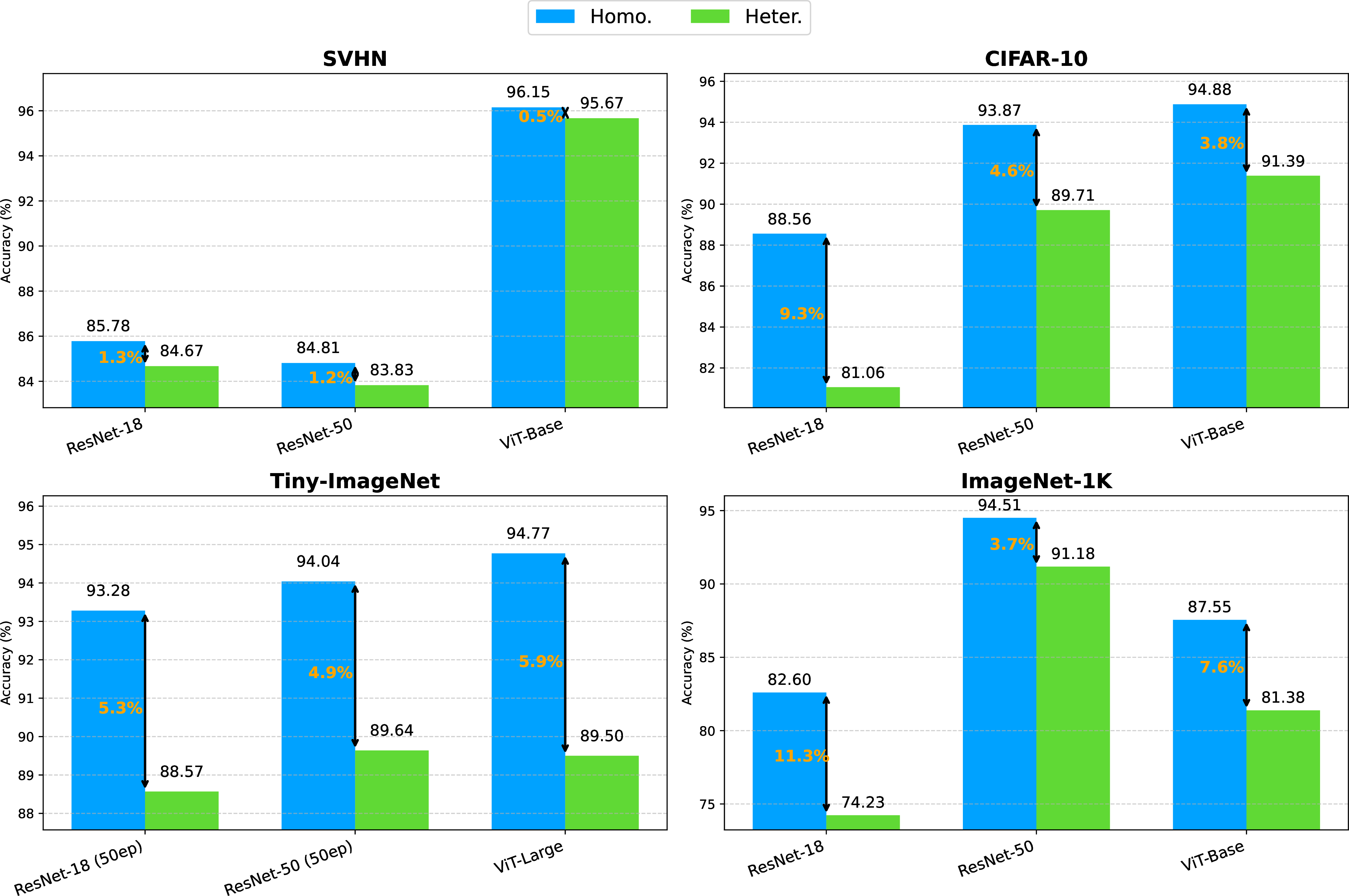
Based on this observation, training discriminators with generative data can be risky, as it may amplify the limitations already present in those trained with real data, further biasing the model toward canonical samples and degrading performance on real data inference.
| Dataset | Model | Link |
|---|---|---|
| SVHN | ResNet-18 | https://huggingface.co/edadaltocg/resnet18_svhn |
| ResNet-50 | https://huggingface.co/edadaltocg/resnet50_svhn | |
| ViT-Base | https://huggingface.co/edadaltocg/vit_base_patch16_224_in21k_ft_svhn | |
| CIFAR-10 | ResNet-18 | https://huggingface.co/SamAdamDay/resnet18_cifar10 |
| ResNet-50 | https://huggingface.co/anonauthors/cifar10-timm-resnet50 | |
| ViT-Base | https://huggingface.co/nateraw/vit-base-patch16-224-cifar10 | |
| Tiny-ImageNet | ResNet-18 | https://github.com/zeyuanyin/tiny-imagenet |
| ResNet-50 | https://github.com/zeyuanyin/tiny-imagenet | |
| ViT-L | https://github.com/ehuynh1106/TinyImageNet-Transformers | |
| ImageNet-1K | All models | timm [75] |
10 Synthetic Data Selection Details↩︎
Following the previous discussion on and , this section introduces our synthetic data selection strategy designed to mitigate the limitations of training discriminators on generative data. The key difference from prior approaches is the incorporation of a diversity score. During selection, in addition to the fidelity score, which measures how closely synthetic samples resemble real data, the diversity score quantifies how far a synthetic instance departs from canonical patterns. As illustrated in Figure 14, when referencing real instances, a synthetic sample receives a higher diversity score if its direction from the set deviates more strongly from the direction toward the canonical pattern.
11 Experiment Details and Full Results↩︎
11.1 Generator usage in the main paper↩︎
To validate our strategy, we train models on synthetic datasets and evaluate them on real data across two settings: in-domain and out-of-domain testing. In these experiments, we utilize publicly available generative models and synthetic dataset, and conduct training using their released code repositories. The corrsponding responses are illustrated in Table 4. For the generator usage in Sec. 4.4, we follow the original papers and use the generators reported in [59], [60]
| Resource | Link |
|---|---|
| Classifiers | |
| SVHN & CIFAR-10 | https://github.com/ML-GSAI/Understanding-GDA |
| Tiny-ImageNet | https://github.com/DennisHanyuanXu/Tiny-ImageNet |
| ImageNet-1K | https://huggingface.co/docs/timm/training_script |
| Generative Models & Data | |
| Synthetic data & code for SVHN, CIFAR, and Tiny-ImageNet | https://github.com/wzekai99/DM-Improves-AT |
| Generator for ImageNet-1K | https://github.com/NVlabs/edm2 |
11.2 IN-1K training recipe↩︎
We use the timm codebase to train models for the IN-1K setting. Since training in IN-1K involves a relatively complex configuration and the final performance can vary with different settings, we report the exact configuration used in the main paper to
facilitate reproduction of our empirical results. We train vit_base_patch16_224 and resnet50 from scratch, and fine-tune vit_base_patch16_224.augreg_in21k and resnetv2_50x1_bit.goog_in21k pretrained on
ImageNet-21K. The concrete settings are shown in Figure 15.
None
Figure 15: Training recipes for different backbones. Top row: from-scratch training. Bottom row: fine-tuning with ImageNet-21K initialization..
11.3 sec:In-domain32classification32accuracy↩︎
Echoing Sec. 4.2, we evaluate model performance on SVHN, CIFAR-10, and Tiny-ImageNet to enable hierarchical assessment across datasets of varying complexity, and further conduct experiments on ImageNet-1K to simulate the large-scale setting.
SVHN: We compare our method with prior approaches, and the results are reported in Table 5. When trained exclusively on synthetic datasets, model performance can surpass that of models trained on real data as the training volume increases. Among different strategies, ours consistently achieves the best performance across varying training data scales.
| Method | 73,257 (Ori. Size) | 80K | 90K | 100K | 200K | 300K |
|---|---|---|---|---|---|---|
| Real Data | 95.84\(\pm\)0.12 | - | - | - | - | - |
| RandSelect [56] | 94.65\(\pm\)0.11 | 94.95 \(\pm\)0.16 | 95.03\(\pm\)0.20 | 95.04\(\pm\)0.13 | 95.78\(\pm\)0.08 | 96.28 \(\pm\)0.13 |
| Clip-Align [4] | 89.14\(\pm\)0.31 | 89.38\(\pm\)0.26 | 89.67\(\pm\)0.23 | 89.67\(\pm\)0.17 | 90.22\(\pm\)0.24 | 90.70 \(\pm\)0.22 |
| RealScore [20] | 94.60\(\pm\)0.12 | 95.03\(\pm\)0.18 | 95.03\(\pm\)0.13 | 95.20\(\pm\)0.16 | 95.72\(\pm\)0.13 | 96.20\(\pm\)0.05 |
| SBSim [21] | 94.71\(\pm\)0.16 | 95.13\(\pm\)0.08 | 95.22\(\pm\)0.12 | 95.25\(\pm\)0.14 | 95.84\(\pm\)0.13 | 96.16\(\pm\)0.06 |
| Ours | 95.44\(\pm\)0.17 | 95.59\(\pm\)0.12 | 95.66\(\pm\)0.11 | 95.83\(\pm\)0.13 | 96.33\(\pm\)0.11 | 96.65\(\pm\)0.04 |
CIFAR-10: We compare our method with prior approaches, and the results are reported in Table 6. When trained exclusively on synthetic datasets, model performance can surpass that of models trained on real data as the training volume increases. Among different strategies, ours consistently achieves the best performance across varying training data scales.
| Methods | 50K (Original Size) | 70K | 90K | 100K | 200K | 300K | 400K | 500K |
|---|---|---|---|---|---|---|---|---|
| Real | 85.80 \(\pm\) 0.73 | - | - | - | - | - | - | - |
| Random | 84.57 \(\pm\) 0.31 | 87.74 \(\pm\)0.48 | 88.73 \(\pm\)0.71 | 89.57\(\pm\)0.25 | 92.78\(\pm\)0.18 | 93.94\(\pm\)0.25 | 94.68 \(\pm\)0.08 | 95.03\(\pm\)0.06 |
| Clip | 77.09\(\pm\)1.19 | 80.97\(\pm\)1.05 | 82.34\(\pm\)0.27 | 82.81\(\pm\)0.67 | 85.62\(\pm\)0.64 | 86.94\(\pm\)0.14 | 87.56\(\pm\)0.29 | 88.39\(\pm\)0.25 |
| Realism | 83.95\(\pm\)1.28 | 87.45\(\pm\)0.58 | 89.03\(\pm\)0.39 | 89.70\(\pm\)0.16 | 92.60\(\pm\)0.30 | 93.92\(\pm\)0.44 | 94.64\(\pm\)0.20 | 94.93\(\pm\)0.11 |
| Similarity | 84.67\(\pm\)0.98 | 87.12\(\pm\)0.70 | 88.72\(\pm\)0.38 | 89.41\(\pm\)0.23 | 91.79\(\pm\)0.23 | 93.21\(\pm\)0.17 | 93.83\(\pm\)0.17 | 94.23\(\pm\)0.13 |
| Ours | 84.96\(\pm\)0.31 | 87.90\(\pm\)0.35 | 89.66\(\pm\)0.40 | 90.47\(\pm\)0.39 | 93.43\(\pm\)0.17 | 94.86\(\pm\)0.20 | 95.45\(\pm\)0.16 | 95.71\(\pm\)0.10 |
Tiny-ImageNet: We compare our method with prior approaches, and the results are reported in Table 7. In this more complex setting, we first train models exclusively on synthetic data, where the performance gap between synthetic- and real-trained models is around 10%. To effectively validate the utility of synthetic data in discriminator training, we use synthetic data as an augmentation to real data. Under this setting, our method consistently outperforms alternatives across different experimental configurations.
| Data Selection Methods | +100K | +200K | +300K | +400K | |
|---|---|---|---|---|---|
| EfficientNet-B0 | Real Data | 73.87 \(\pm\) 0.29 | – | – | – |
| RandSelect [56] | 74.16 \(\pm\) 0.25 \((+0.29)\) | 74.59 \(\pm\) 0.28 \((+0.29)\) | 75.00 \(\pm\) 0.21 \((+1.13)\) | 75.70 \(\pm\) 0.14 \((+1.70)\) | |
| CLIP-Align [4] | 60.54 \(\pm\) 0.42 \((-13.33)\) | 62.24 \(\pm\) 0.50 \((-11.63)\) | 62.59 \(\pm\) 0.36 \((-11.28)\) | 63.13 \(\pm\) 0.05 \((-10.74)\) | |
| RealScore [20] | 74.66 \(\pm\) 0.27 \((+0.79)\) | 75.67 \(\pm\) 0.19 \((+1.90)\) | 75.80 \(\pm\) 0.14 \((+1.93)\) | 76.60 \(\pm\) 0.04 \((+2.73)\) | |
| MaxSim (\(\alpha=0\)) [21] | 74.69 \(\pm\) 0.09 \((+0.82)\) | 75.11 \(\pm\) 0.25 \((+1.24)\) | 75.48 \(\pm\) 0.29 \((+1.61)\) | 75.94 \(\pm\) 0.16 \((+2.07)\) | |
| MaxDiv (\(\alpha=1\)) | 74.93 \(\pm\) 0.11 \((+1.06)\) | 75.59 \(\pm\) 0.11 \((+1.72)\) | 75.90 \(\pm\) 0.11 \((+2.03)\) | 76.23 \(\pm\) 0.05 \((+2.36)\) | |
| Ours | 75.03 \(\pm\) 0.18 \((+1.16)\) | 75.91 \(\pm\) 0.06 \((+2.04)\) | 76.65 \(\pm\) 0.14 \((+2.78)\) | 76.86 \(\pm\) 0.14 \((+2.99)\) | |
| ResNet-50 | Real Data | 64.13 \(\pm\) 0.67 | – | – | – |
| RandSelect [56] | 66.55 \(\pm\) 0.24 \((+2.42)\) | 68.32 \(\pm\) 0.25 \((+4.19)\) | 69.45 \(\pm\) 0.42 \((+5.32)\) | 70.41 \(\pm\) 0.21 \((+6.28)\) | |
| CLIP-Align [4] | 53.12 \(\pm\) 0.88 \((-11.01)\) | 55.16 \(\pm\) 0.38 \((-8.97)\) | 56.97 \(\pm\) 0.30 \((-7.16)\) | 58.30 \(\pm\) 0.25 \((-5.83)\) | |
| RealScore [20] | 66.05 \(\pm\) 0.45 \((+1.92)\) | 69.12 \(\pm\) 0.11 \((+4.99)\) | 70.09 \(\pm\) 0.19 \((+5.96)\) | 71.51 \(\pm\) 0.11 \((+7.38)\) | |
| SBSim (\(\alpha=0\)) [21] | 65.69 \(\pm\) 0.35 \((+1.56)\) | 67.12 \(\pm\) 0.57 \((+2.99)\) | 70.10 \(\pm\) 0.37 \((+5.97)\) | 71.26 \(\pm\) 0.42 \((+7.13ß)\) | |
| Diversity (\(\alpha=1\)) | 65.87 \(\pm\) 0.50 \((+1.74)\) | 68.16 \(\pm\) 0.25 \((+4.03)\) | 70.12 \(\pm\) 0.13 \((+5.99)\) | 72.52 \(\pm\) 0.21 \((+8.39)\) | |
| Ours | 68.57 \(\pm\) 0.19 \((+4.44)\) | 70.82 \(\pm\) 0.08 \((+6.69)\) | 71.80 \(\pm\) 0.26 \((+7.67)\) | 73.05 \(\pm\) 0.25 \((+8.92)\) |
11.4 Out-of-domain classification accuracy↩︎
Assessing models’ robustness, OOD evaluations are implemented ( Sec. 4.3 in main paper). We report the concrete performance values in each setting as blow:
SVHN: We evaluate OOD performance using the extra split of SVHN [48] and test subset of distorted SVHN. Detailed results are presented in Table [tbl:tab:SVHN95OOD].
| Method | SVHN | SVHN-Extra | SVHN-test-small-collage | SVHN-test-middle-collage | SVHN-test-strong-collage | SVHN-test w/large-collage | SVHN-Extra w/large-collage |
|---|---|---|---|---|---|---|---|
| Real Data | 95.90 | 98.09 | 93.53 | 86.24 | 80.20 | 72.15 | 75.68 |
| RandSelect | 96.19 | 98.20 | 93.85 | 86.52 | 80.92 | 73.35 | 77.27 |
| SBSim | 96.25 | 98.22 | 94.04 | 86.79 | 80.63 | 72.16 | 76.29 |
| Clip-Align | 87.21 | 92.77 | 83.97 | 73.26 | 63.83 | 54.37 | 60.87 |
| RealScore | 96.25 | 98.20 | 93.86 | 86.47 | 80.86 | 73.09 | 77.04 |
| Ours | 96.66 | 98.45 | 94.42 | 87.41 | 81.50 | 73.96 | 77.76 |
CIFAR-10: We use CIFAR-10-Warehouse [69] as a benchmark, the subset of data in this benchmark is illustrated in Figure 16. The inference results are presented in Table 9.
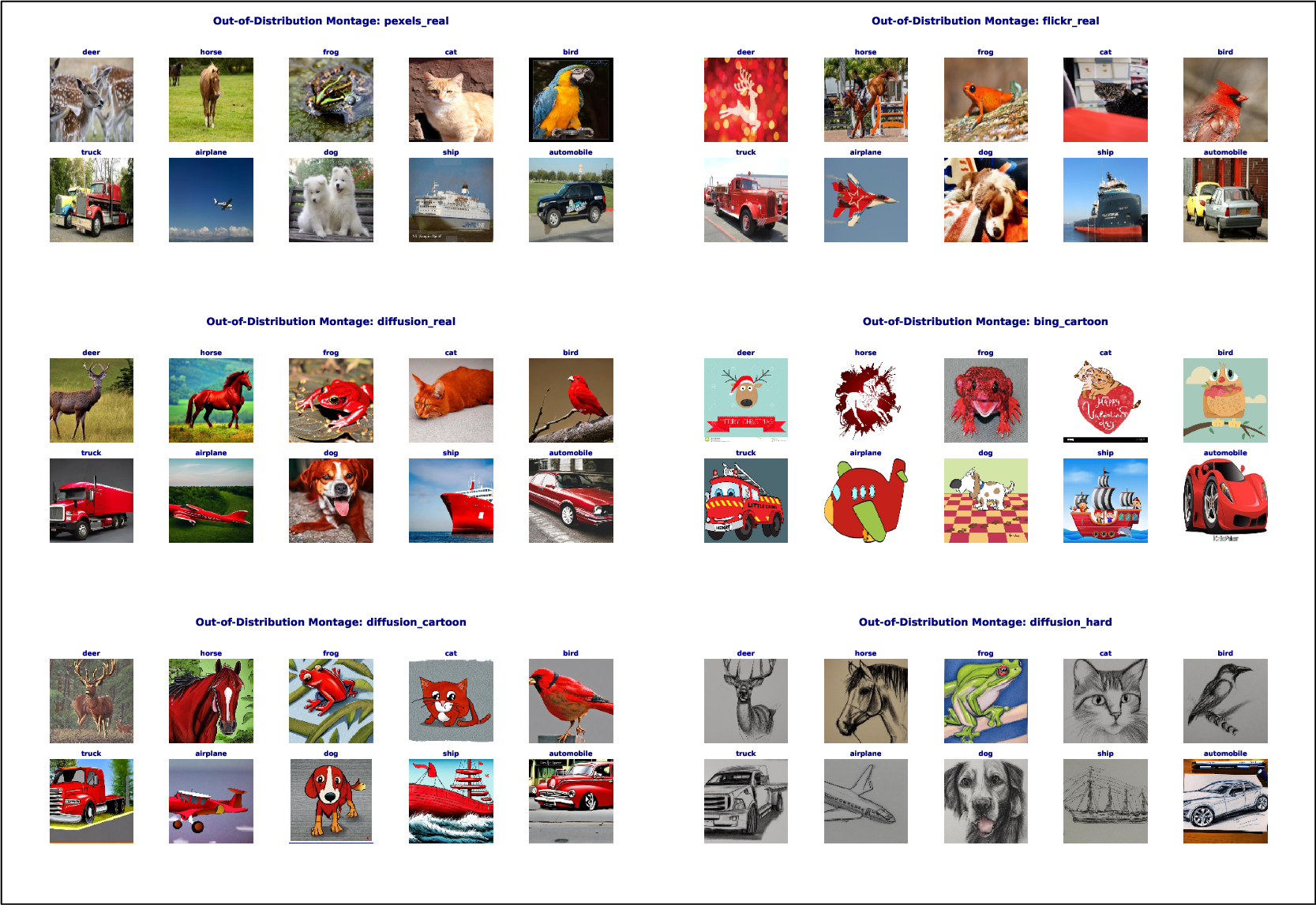
| Method | Diffusion | Flickr | Pexels | 360 |
|---|---|---|---|---|
| Original | 0.819 | 0.708 | 0.810 | 0.547 |
| Random Sampling | 0.904 | 0.819 | 0.908 | 0.655 |
| Similar Only | 0.914 | 0.820 | 0.908 | 0.663 |
| CLIP | 0.932 | 0.797 | 0.898 | 0.660 |
| Realism | 0.924 | 0.831 | 0.920 | 0.679 |
| Ours | 0.934 | 0.850 | 0.935 | 0.709 |
Tiny-ImageNet: We utilize Tiny-ImageNet-C [64] for the evaluation of OOD, which incorporates various types of corruption. We classify them into three types: color-variation set (brightness adjustment, contrast variation), noise-variation set (pixelation, Gaussian noise, motion blur), and compression-variation set (JPEG compression). The results are presented in Table 10.
| Method | Color | Noise | Compression |
|---|---|---|---|
| Original | 40.52 | 46.94 | 48.33 |
| Random Sampling | 48.17 | 46.13 | 54.23 |
| Similar Only | 48.40 | 53.62 | 56.89 |
| CLIP | 40.52 | 39.73 | 40.12 |
| Realism | 49.41 | 52.57 | 54.23 |
| Ours | 52.19 | 58.77 | 61.86 |
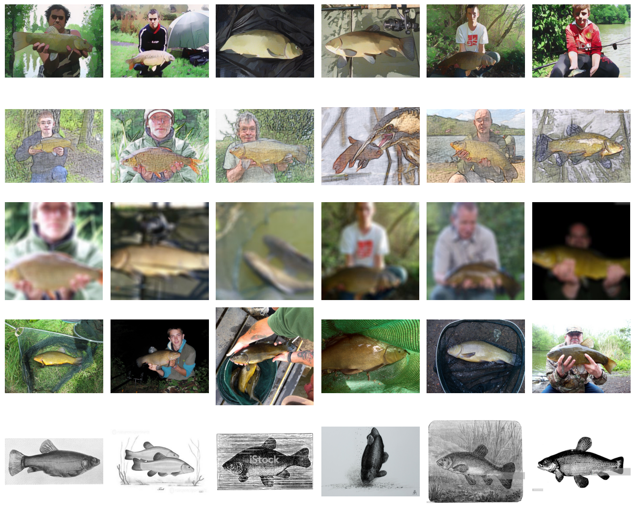
ImageNet-1K: We use five ImageNet-1K OOD, illustrated in Figure 17:
1) ImageNet-V2 [65] is constructed to closely match the distribution of the original ImageNet-1K, containing 50,000 images across the same 1,000 classes as the original validation set.
2) ImageNet-Sketch [66] consists of black-and-white sketches covering all ImageNet-1K classes, with 50 images per class.
3) ImageNet-C [67] evaluates model robustness to common corruptions such as noise, blur, weather effects, and digital distortions by applying perturbations with severity levels from 1 to 5 to the original ImageNet validation images.
4) ImageNet-Drawing [68] is derived from the ImageNet validation set, where images are transformed into drawing styles using generative adversarial networks and image processing techniques.
5) ImageNet-Cartoon [68] is also derived from the ImageNet validation set, where images are transformed into cartoon styles.
We categorize them into two main groups based on the sources of image. 1) Original OOD: ImageNet-V2 and ImageNet-Sketch; 2) Derivative OOD: ImageNet-C, ImageNet-Drawing and ImageNet-Cartoon. The inference results is illustrated in the Table 11, 12.
| Method | IN-V2-freq. | IN-Sketch | IN-Cartoon | IN-Drawing | IN-C (gaussian) | IN-C (motion) | IN-C (jpeg) | IN-C (snow) |
|---|---|---|---|---|---|---|---|---|
| Original | 49.86 | 11.213 | 43.36 | 17.494 | 18.434 | 30.774 | 47.668 | 29.476 |
| Random Sampling | 60.57 | 23.826 | 58.974 | 27.728 | 35.51 | 41.136 | 61.364 | 40.986 |
| SBSim | 60.16 | 23.3 | 58.554 | 29.342 | 33.258 | 39.736 | 61.158 | 39.952 |
| CLIP-Align | 56.3 | 21.193 | 56.276 | 32.686 | 35.086 | 38.16 | 58.296 | 38.08 |
| Realism | 60.61 | 23.73 | 58.93 | 27.75 | 35.48 | 41.2 | 61.31 | 40.88 |
| Ours | 61.25 | 25.308 | 59.65 | 30.138 | 37.226 | 43.394 | 62.18 | 42.666 |
| Method | IN-V2-freq. | IN-Sketch | IN-Cartoon | IN-Drawing | IN-C (gaussian) | IN-C (motion) | IN-C (jpeg) | IN-C (snow) |
|---|---|---|---|---|---|---|---|---|
| Original | 56.98 | 17.34 | 41.852 | 14.948 | 11.418 | 22.78 | 41.552 | 22.46 |
| Random Sampling | 60.78 | 25.29 | 55.27 | 26.054 | 31.518 | 26.152 | 53.132 | 35.906 |
| SBSim | 58.81 | 24.378 | 52.118 | 24.762 | 28.18 | 25.774 | 50.156 | 30.628 |
| CLIP-Align | 56.45 | 24.201 | 49.996 | 24.956 | 27.188 | 22.928 | 49.212 | 27.722 |
| Realism | 60.78 | 25.3 | 55.25 | 26.044 | 31.6 | 26.13 | 53.135 | 35.906 |
| Ours | 61.76 | 26.77 | 55.404 | 26.16 | 35.458 | 25.93 | 52.98 | 34.29 |
| Dataset | Generator | Synthetic Data Size | Classifier | Training Size |
|---|---|---|---|---|
| CIFAR-10 | EDM | 1M | ResNet-18 | 100K |
| ImageNet-100 | EDM2 | 1M | ResNet-50 | 120K |
8pt
12 Additional Analysis↩︎
12.1 Limitation of CLIP filter↩︎
Reviewing the experimental results, we observe that using CLIP as a filter to select synthetic data consistently leads to the worst performance when training discriminators. Upon inspecting the selected samples, we attribute this degradation to the dominance of monotonous instances. As illustrated in Figure 18, high- and low-CLIP-score examples in Tiny-ImageNet generated by EDM highlight this issue, while Figure 19 presents corresponding cases in ImageNet-1K generated by EDM2. When constructing datasets from a synthetic pool, prioritizing high-CLIP-score instances produces collections enriched with canonical patterns but lacking diversity, ultimately resulting in weaker performance on both in-domain and out-of-domain evaluations.


12.2 Feature Extractor Ablation↩︎
Our strategy is built upon image feature representations; therefore, we further investigate whether the choice of feature extractor influences the final performance of classifiers. In this ablation study, we conduct experiments on two datasets: CIFAR-10 and ImageNet-100. The experimental configurations are summarized in Table 13. Specifically, for CIFAR-10, we use EDM to generate 1M synthetic samples and apply our strategy to select 100K training instances, which are then used to train a ResNet-18 model.
13 Implement Details↩︎
13.1 Code:32scoring↩︎
Listing lst:alignment: Synthetic alignment scoring
def compute_synthetic_common_alignment_scores(
    syn_normed,               # [N, D]  normalized synthetic features
    real_common_normed        # [M_1, D] normalized real-common
    synthetic_common_fidelity = syn_normed @ real_common_normed.T

    # diversity score
    centroid_common = F.normalize(real_common_normed.mean(dim=0, keepdim=True), dim=1)
    A = syn_normed.unsqueeze(1) - real_common_normed.unsqueeze(0)  # [N, M_1, D]
    B = centroid_common - real_common_normed  # [M_1, D]
    numerator = (A * B.unsqueeze(0)).sum(dim=-1)      # [N, M_1]
    A_norm = A.norm(dim=-1)                           # [N, M_1]
    B_norm = B.norm(dim=-1).unsqueeze(0)              # [1, M_1]

    synthetic_common_diversity = numerator / (A_norm * B_norm + 1e-8)  # [N, M_1]
    synthetic_common_score = synthetic_common_fidelity - synthetic_common_diversity  # [N, M_1]
    return synthetic_common_fidelity, synthetic_common_diversity, synthetic_common_score

def compute_synthetic_rare_alignment_scores(
  syn_normed = None, real_rare_normed = None,
  real_np = None,  # real features matrix
  class_rare_2_common_in_real_dict = None  ):
  synthetic_rare_fidelity = syn_normed @ real_rare_normed.T  # [N, M_2]

  rare_2_common_in_real_dict = class_rare_2_common_in_real_dict

  common_counterpart_index = [i["common_image"] for i in rare_2_common_in_real_dict.values()]

  common_counterpart_matrix = get_real_subset_features_matrix(real_np, common_counterpart_index)  # [M_2, D]
  normalized_common_counterpart_matrix = F.normalize(common_counterpart_matrix, dim=1)  # [M_2, D]

  rare_2_common_matrix = normalized_common_counterpart_matrix - real_rare_normed  # shape: [M2, D]
  norm_rare_2_common_matrix = rare_2_common_matrix / rare_2_common_matrix.norm(dim=-1, keepdim=True)  # Normalize to unit vectors

  rare_2_synthetic_matrix = syn_normed.unsqueeze(1) - real_rare_normed.unsqueeze(0)  # [N, M2, D]
  norm_rare_2_synthetic_matrix = rare_2_synthetic_matrix / rare_2_synthetic_matrix.norm(dim=-1, keepdim=True)  # [N, M2, D]

  cos_sim_matrix = (norm_rare_2_synthetic_matrix * norm_rare_2_common_matrix.unsqueeze(0)).sum(dim=-1)
  synthetic_rare_diversity = cos_sim_matrix  # [N, M2]
  synthetic_rare_score = synthetic_rare_fidelity - synthetic_rare_diversity  # [N, M2]
  return synthetic_rare_fidelity, synthetic_rare_diversity, synthetic_rare_score
13.2 sec:Code:32selection↩︎
Listing lst:topk_synthetic: Top-k synthetic selection
def get_the_highest_score_index(matrix, synthetic_name_list, top_k=250, top_n=2, reverse=False):
    if matrix.shape[0] > matrix.shape[1]:
        matrix = matrix.T
        number_of_real = matrix.shape[0]
        number_of_synthetic = matrix.shape[1]
    if reverse:
        matrix = -matrix

    # for each row return the top-n largest column indices and values
    topk_values, topk_indices = torch.topk(matrix, top_n, dim=1)  # shape: (rows, top_n)
    # print("the shape of matrix:", matrix.shape)
    assert len(synthetic_name_list) == matrix.shape[1], \;
        "Synthetic image names length must match the number of synthetic features."

    retrieval_syn_image_and_scores = {}
    # iterate through each row
    for indices, values in zip(topk_indices, topk_values):
        for idx, val in zip(indices, values):
            current_image_name = synthetic_name_list[idx.item()]
            current_value = retrieval_syn_image_and_scores.get(current_image_name, -9999)
            if val.item() > current_value:
                retrieval_syn_image_and_scores[current_image_name] = val.item()
    # check unique count
    assert len(set(retrieval_syn_image_and_scores.keys())) >= top_k, \;
        f"The number of unique top-{top_n} column indices is less than top_k."
    return list(retrieval_syn_image_and_scores.keys()), retrieval_syn_image_and_scores
14 Limitations↩︎
This work has several limitations, which also point to promising directions for future research.
1) Dependence on generator quality. Our method operates as a post-generation curation strategy built on top of off-the-shelf generators, without intervening in or steering the generation process itself. As a result, the upper bound of synthetic data utility is inherently constrained by the quality of the generator. When the generator is too weak to produce realistic images, curation may largely reduce to selecting samples with relatively higher fidelity, while diversity-aware selection may become less beneficial because low-fidelity samples can further weaken downstream performance. Nevertheless, as modern generative models continue to improve, synthetic data is becoming increasingly realistic, making post-generation curation more meaningful for unlocking its downstream utility.
2) Limited to unimodal image settings. Our current method focuses on curating synthetic image data and does not extend to multimodal settings. As vision-language models continue to advance, synthetic datasets that support multimodal training are becoming increasingly important. However, multimodal curation involves data formats beyond images and requires modeling interactions across modalities, which are not addressed by the current framework. Extending post-generation curation to multimodal data is therefore an important and meaningful direction for future work.
3) Reliance on real reference data. Our method requires a real reference set to construct the \(\mathcal{I}_{HO}\)/\(\mathcal{I}_{HE}\) partition, which is standard in reference-based curation. In practice, however, only a small reference set is often sufficient, since the partition depends more on relative intra-class similarity than on absolute data scale.
4) Dependence on pretrained feature extractors. Our scoring procedure relies on pretrained feature extractors. Although Fig. 9 shows that the method is only modestly sensitive to the choice of encoder, a severely domain-mismatched feature extractor may still degrade partition quality. In practice, we recommend using strong general-purpose encoders, such as SigLIP, when domain-specific alternatives are unavailable.
15 sec:Broader32impacts↩︎
Our work on synthetic data selection raises several ethical considerations that warrant discussion. Bias Amplification: Our HOMO-HETERO partitioning strategy could potentially amplify biases present in the original data if the HOMO set disproportionately represents certain demographic groups or patterns. We mitigate this by explicitly incorporating diversity metrics in our selection criteria. Environmental Impact: While synthetic data generation incurs computational costs, our selective curation approach reduces the environmental footprint by enabling comparable performance with smaller datasets, requiring fewer training iterations and less storage. Privacy Preservation: Although synthetic data generally poses fewer privacy risks than real data, our method does not specifically filter for instances that might inadvertently resemble real individuals. Practitioners should implement additional privacy checks when deploying our method in sensitive domains. Responsible Use: We acknowledge that synthetic data technology could be misused for creating deceptive content. Our method is designed for legitimate research and educational purposes, specifically to improve model training efficiency while maintaining performance standards. We encourage adherence to established guidelines for synthetic data use and advocate for continued development of detection methods to distinguish synthetic from real content.
References↩︎
Corresponding author.↩︎