GLM-5 Serving Parameter Tuning for OpenClaw
Single-Deployment MaaS Inference Optimization for Long-Context Agent Workloads
April 27, 2026
huamj5@chinaunicom.cn, wangn85@chinaunicom.cn, yangpj16@chinaunicom.cn
wangk115@chinaunicom.cn, liansg@chinaunicom.cn
Abstract
OpenClaw requests are dominated by long, tool-augmented prefixes: a sizable system prompt, accumulated conversation history, and tool outputs that are fed back into the context window [1], [2]. Under this workload shape—approximately 28000 to 30000 input tokens per request and about 500 output tokens—serving quality is governed jointly by throughput, time-to-first-token (TTFT), and tail latency rather than by raw short-prompt throughput alone [3], [4].
This report positions the tuning work inside a Model-as-a-Service (MaaS) multi-model inference optimization architecture. The broader architecture spans domain applications, MaaS platform performance optimization, multi-model orchestration, inference optimization, and compute-stack adaptation; the scope of this report is the Single-Node Optimization block in the inference-optimization layer, where serving parameters such as chunked prefill, tensor parallelism (TP), pipeline parallelism (PP), and max-running-request concurrency are tuned for one GLM-5 serving deployment. In this report, Single-Node Optimization is the architecture-block label, not a restriction to one physical server; the measured deployment uses the two-node, sixteen-GPU cluster described in Section 4.
Within the tested parameter space, the best measured configuration is chunked-prefill-size=3072, tp=4, pp-size=4, and max-running-requests=24. Relative to the conservative 2048/4/4/16
baseline, this setting improves request throughput from 0.43 to 0.48 req/s and total token throughput from 9029.64 to 9993.23 tok/s, while reducing TTFT average from 8.98 to 6.69 seconds and latency P90 from 40.23 to 32.64 seconds. Under a fixed hardware
footprint, that corresponds to an estimated 10.4% lower serving cost per request and 9.6% lower serving cost per token. Relative to the 4096/4/4/16 comparison profile, normalized serving cost falls by about 20.8% per request and 21.1% per
token.
Accordingly, we recommend 3072 / tp4 / pp4 / max24 as the default deployment profile for OpenClaw. The data also show that the optimum is not monotonic: larger chunk sizes (4096, 6144) and deeper queueing
(32, 48) do not further improve this workload. The results indicate a workload-specific sweet spot rather than a simple “larger is always better” rule.
1 Background and Problem Definition↩︎
Optimizing serving parameters using “raw model throughput” (e.g., short prompts, single-turn, synthetic load) can be misleading for OpenClaw. OpenClaw constructs a per-run context that includes: (i) a system prompt describing tools/skills/runtime constraints, (ii) the full conversation history, and (iii) tool calls and tool outputs; all of these consume tokens inside the model context window [1], [2]. As a result, even when the user prompt is brief, the effective model input can become very long, especially as multi-turn interactions accumulate and tool outputs (command output, file snippets, web/tool results) are reinjected [1].
This yields three business-relevant characteristics for OpenClaw agent serving:
Long system prompt and high context overhead. Tool schemas and injected workspace content add non-trivial context cost each turn [2]. This increases the probability of “long prefix” requests even in routine usage.
Multi-turn accumulation and tool-heavy traces. Multi-round agent sessions are inherently prefix-growing: each turn appends assistant outputs and tool transcripts [1]. Long-prefix requests make prefill time and KV-cache pressure first-order performance factors [5].
Interactive stability over peak throughput. In an agent product, user experience is driven by responsiveness (TTFT) and predictability (tail latency), not by maximizing requests-per-second at the cost of jitter and queueing [3], [4]. Over-aggressive batching can turn the endpoint into a throughput-first queueing system, where some requests wait much longer before streaming begins.
Given this workload, three parameters become especially critical:
Chunked prefill size. SGLang exposes --chunked-prefill-size to control the maximum tokens per prefill chunk [6]. This directly affects how long prefixes are partitioned, which in turn influences prefill efficiency, interference with decode, and observed TTFT under load.
Tensor parallelism and pipeline parallelism. --tp-size and --pp-size determine how the model computation is split across devices [6]. TP trades compute locality for collective communication (as in Megatron-style tensor model parallelism), while PP introduces pipeline scheduling and potential “bubble” overhead that
depends on stage balance and micro-batching [7]–[9].
Max running requests. --max-running-requests caps the number of running requests and thereby constrains effective batch size and queue depth [6]. It is a primary knob for throughput versus latency stability; SGLang guidance explicitly frames it as a control surface for memory safety and batching behavior [10].
2 MaaS Multi-Model Inference Optimization Architecture↩︎
Figure 1 shows the MaaS Multi-Model Inference Optimization Architecture that frames this report. The architecture is organized as a five-layer stack: an application layer for domain-facing workloads, a platform layer for MaaS performance optimization, an orchestration layer for multi-model fusion, an inference optimization layer for request scheduling and model-serving efficiency, and a compute adaptation layer for accelerator- and toolchain-specific execution. This report focuses on the Single-Node Optimization block in the inference optimization layer, especially TP/PP parameter tuning and the adjacent serving controls that determine prefill behavior and request concurrency.
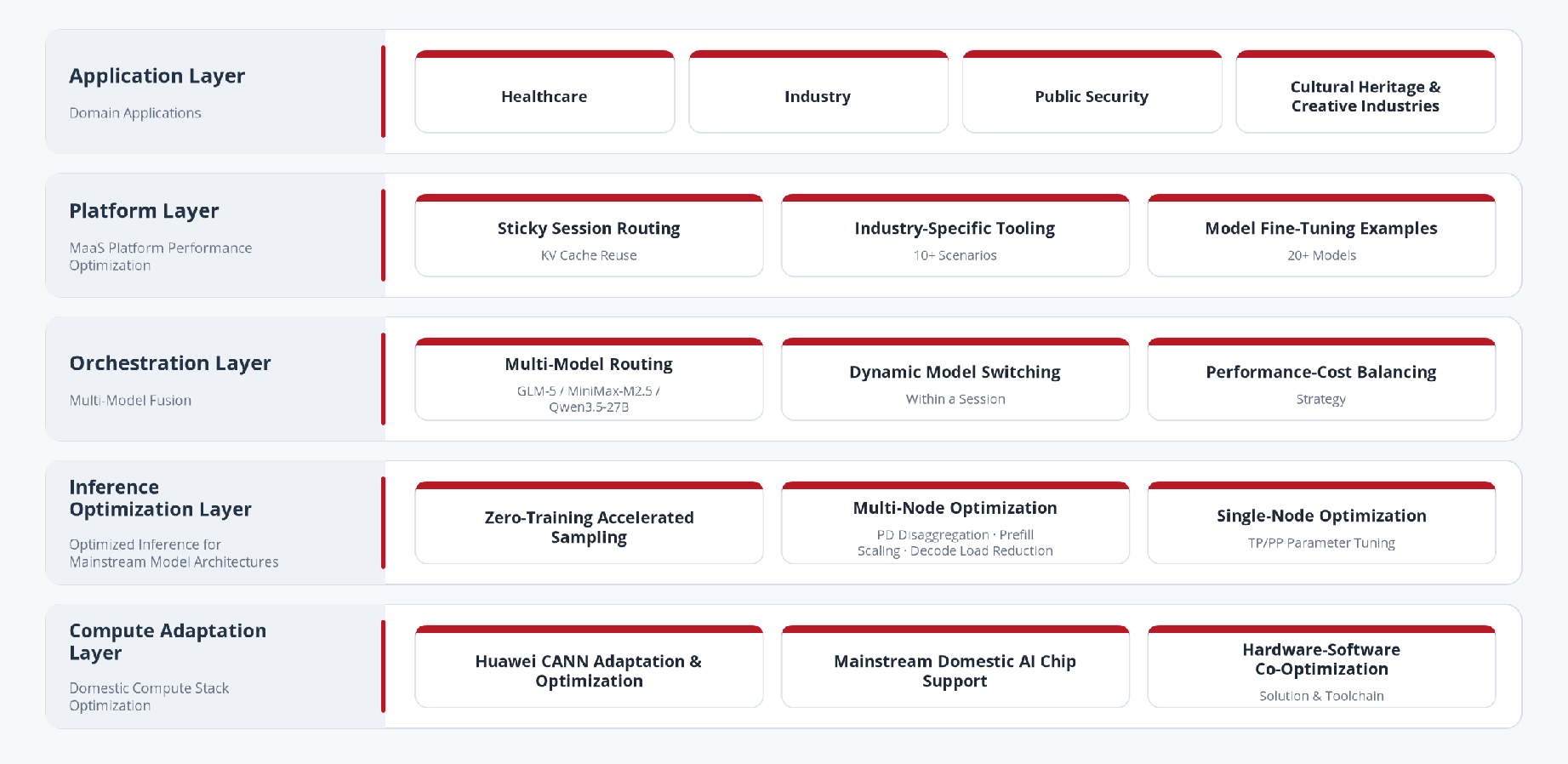
The application layer captures the domain workloads served by the MaaS platform. In the illustrated architecture, these workloads include healthcare, industry, public security, and cultural heritage/creative-industry applications. This layer is important because each domain can produce different prompt shapes, safety constraints, latency targets, and tool-use patterns. For OpenClaw, the dominant workload shape is a long-context agent session rather than a short single-turn prompt, so the serving profile must be optimized for large prefills and interactive streaming latency.
The platform layer represents MaaS platform performance optimization. Its mechanisms include sticky session routing for KV-cache reuse, industry-specific tooling, and model fine-tuning examples. Sticky session routing is especially relevant for long-context agents: when requests from the same session are routed consistently, repeated prefixes and accumulated session context can be reused more effectively, reducing avoidable recomputation and improving TTFT stability. The tooling and fine-tuning components provide the surrounding platform capabilities needed to specialize the MaaS service for multiple application domains.
The orchestration layer implements multi-model fusion. The architecture explicitly includes multi-model routing across models such as GLM-5, MiniMax-M2.5, and Qwen3.5-27B, dynamic model switching within a session, and performance–cost balancing. These functions decide which model should serve a request or a session segment. This report does not tune cross-model routing policies; instead, it holds model selection fixed to the GLM-5 serving path so that the impact of single-deployment serving parameters can be measured cleanly.
The inference optimization layer is the main technical layer for this study. It contains zero-training accelerated sampling, multi-node optimization, and single-node optimization. The multi-node branch covers mechanisms such as
prefill/decode disaggregation, prefill scaling, and decode-load reduction. The single-node branch covers TP/PP parameter tuning, which is the direct focus of the present work. In addition to TP/PP, the experiments tune chunked-prefill-size and
max-running-requests, because these parameters determine how long-prefix requests are partitioned, admitted, and batched before decoding begins.
The compute adaptation layer maps the optimized inference workload onto the available compute stack. The architecture includes Huawei CANN adaptation and optimization, mainstream domestic AI chip support, and hardware–software co-optimization through solution and toolchain work. Although the measurements in this report are collected on the fixed experimental hardware described later, the role of this layer is to ensure that the same optimization method can be adapted to different accelerator backends and deployment toolchains.
In this report, Single-Node Optimization refers to optimizing one GLM-5 serving deployment path while holding the higher-level MaaS routing and multi-model orchestration policies constant. It should not be interpreted as a claim that the
measured hardware footprint is limited to one physical server; rather, it identifies the architectural scope of the work: local serving-parameter tuning for a single model-serving path. The recommended 3072 / tp4 / pp4 / max24 profile should
therefore be read as the best tested single-deployment configuration for the OpenClaw long-context workload under the measured environment.
3 Methodology↩︎
This section defines the workload abstraction, evaluation metrics, and controlled-comparison protocol used to study serving-parameter sensitivity for OpenClaw.
Benchmark workload and traffic abstraction. The objective of the benchmark is not to maximize synthetic short-prompt throughput, but to approximate the request shape of OpenClaw online traffic, which is dominated by
long system prompts, accumulated conversation history, and tool-returned context [1]. To reflect this property, the experiments use
SGLang bench_serving with a long-input synthetic profile rather than a short-context microbenchmark. A representative command uses --dataset-name random, --random-input-len 30000,
--random-output-len 500, and --random-range-ratio 0.2, together with the same model and tokenizer path as the online deployment. Under this setup, the generated requests have an average input length of approximately 28000–30000
tokens and an average output length of approximately 500 tokens. This workload construction is a deliberate abstraction: it does not replay production traces token by token, but it preserves the dominant systems characteristic relevant to this
study—very long prefills with moderate decode length. That choice makes the benchmark suitable for answering the report’s central question, namely which server parameters best balance throughput and latency for the OpenClaw long-context serving
regime.
Evaluation metrics and interpretation. The current sweep records the following directly measured metrics from the benchmark output [3]: (i) output token throughput (tok/s), (ii) total token throughput (tok/s), (iii) request throughput (req/s), (iv) average TTFT, (v) TTFT P90, (vi) average TPOT, and (vii) end-to-end latency P90. Together, these metrics capture both system efficiency and user-perceived responsiveness. Throughput metrics quantify hardware utilization under sustained load, while TTFT and percentile latency characterize interactivity and stability under queueing pressure [4], [11]. The analysis centers on fields directly reported by the benchmark output. Metrics such as average end-to-end latency, ITL, or P99 latency are not introduced unless they are explicitly available, which avoids overstating precision or fabricating unsupported comparisons.
Methodological principle. The study follows a controlled-comparison design: keep the deployment platform, model artifact, and software stack fixed; vary only the serving parameters of interest; and evaluate each candidate under a workload that reflects the long-context characteristics of OpenClaw. The study does not claim a universal optimum for GLM-5 serving. Rather, it identifies the most effective configuration within the tested parameter space for a specific production-like workload running on a specific FP8 model artifact and a specific two-node H100 cluster.
Benchmark provenance and reproducibility scope. The raw sweep values used in Table 1, Figure 2, Figure 3, and Table 2 are taken from the internal GLM-5 serving stress-test log for the OpenClaw long-context workload [12]. Each row in the raw CSV corresponds to one aggregate bench_serving measurement for a single server configuration. The available log records aggregate throughput and latency metrics but does not include
repeated-run identifiers, a random seed, or a warm-up duration; consequently, this report does not claim confidence intervals or statistical significance. All recommendations are therefore phrased as best measured within the tested parameter space
under the fixed hardware and software environment, not as a universal optimum for GLM-5 serving.
4 Experiments↩︎
4.1 Experimental Setup↩︎
This section describes the experimental platform, model artifact, and serving stack used for the parameter sweep.
Testbed and hardware configuration. All measurements were collected on the same distributed serving cluster so that parameter comparisons are made under a fixed hardware budget. The deployment platform consists of a two-node,
sixteen-GPU H100 cluster, with eight H100 GPUs per node. Each server is equipped with 2\(\times\) Intel Xeon Platinum 8468 CPUs (48 cores per socket, for 96 physical cores and 192
hardware threads per node) and 2 TiB of system memory. Local storage is organized as 2\(\times\) 1.7 TB Samsung SATA SSDs in RAID1 for the system volume, together with 8\(\times\) 7 TB Intel NVMe SSDs for high-throughput data access and benchmark staging. The I/O and network inventory includes multiple Mellanox ConnectX-7 InfiniBand adapters, as well as Intel
E810-XXV and Mellanox ConnectX-6 Dx Ethernet controllers. This hardware context is important for interpreting the parallelism study, because the tested tp/pp decompositions—2/8, 4/4, and
8/2—all consume the same sixteen accelerators but induce different collective-communication and pipeline-balance demands on the interconnect fabric [9]. By fixing CPU, memory, storage, and network configuration across the entire sweep, the study isolates the effect of serving parameters rather than mixing them with host-level
resource variation.
| Block / role | chunk | tp | pp | max-run | Out tok/s | Total tok/s | Req/s | TTFT avg | TTFT P90 | TPOT ms | Latency P90 |
|---|---|---|---|---|---|---|---|---|---|---|---|
| Chunk | 2048 | 4 | 4 | 16 | 215.17 | 9029.64 | 0.43 | 8.98 | 14.18 | 54 | 40.23 |
| Chunk best (max16) | 3072 | 4 | 4 | 16 | 220.89 | 9269.88 | 0.44 | 8.04 | 12.58 | 54 | 40.07 |
| Chunk | 4096 | 4 | 4 | 16 | 187.90 | 7885.54 | 0.38 | 9.73 | 17.39 | 63 | 51.98 |
| Chunk | 6144 | 4 | 4 | 16 | 202.62 | 8503.08 | 0.41 | 8.85 | 15.00 | 59 | 44.97 |
| Global winner | 3072 | 4 | 4 | 24 | 238.13 | 9993.23 | 0.48 | 6.69 | 11.61 | 50 | 32.64 |
| Queue | 3072 | 4 | 4 | 32 | 235.55 | 9885.18 | 0.47 | 7.01 | 12.07 | 50 | 33.21 |
| Queue | 3072 | 4 | 4 | 48 | 231.16 | 9701.02 | 0.46 | 7.39 | 12.87 | 50 | 34.03 |
| 4096/max32 check | 4096 | 4 | 4 | 32 | 225.47 | 9462.00 | 0.45 | 7.73 | 12.90 | 51 | 36.01 |
| TP/PP | 3072 | 2 | 8 | 24 | 207.43 | 8705.06 | 0.41 | 7.80 | 12.96 | 57 | 37.41 |
| TP/PP | 3072 | 8 | 2 | 24 | 164.56 | 6905.99 | 0.33 | 9.48 | 16.50 | 73 | 47.55 |
4.0pt
Model artifact and precision scope. The serving target is the GLM-5 FP8 checkpoint. Accordingly, all benchmark results in this report characterize the FP8 deployment variant of GLM-5 on the current H100 cluster. Quantization changes the model weight footprint and therefore the amount of GPU memory that remains available for long-context KV cache and for concurrent requests. It can also change runtime behavior indirectly through kernel selection, memory-fragmentation patterns, and communication pressure in distributed execution [5], [13]. For that reason, the recommended parameter setting derived in this report should not be over-generalized to BF16, INT4, W4A8, or other GLM-5 artifacts without separate measurement. The conclusions here are intentionally narrower: they identify the best tested serving configuration for the FP8 OpenClaw deployment under the present hardware conditions.
Serving stack and controlled variables. The online service is implemented with SGLang v0.5.9 in two-node distributed mode and uses the flashinfer attention backend. Across all experiments, the fixed
server-side settings include --nnodes 2, --served-model-name glm-5, --trust-remote-code, --tool-call-parser glm47, --reasoning-parser glm45, --enable-reasoning-tokens,
--context-length 202752, --mem-fraction-static 0.85, --enable-metrics, and --enable-cache-report. Only three serving knobs are intentionally varied in the sweep: --chunked-prefill-size, the
tensor/pipeline parallelism split (tp/pp), and --max-running-requests. This experimental design provides a clean basis for comparison: the model artifact, cluster topology, and serving framework are held constant, so performance
differences can be attributed directly to the scheduling and partitioning choices under study [6].
5 Ablation Study↩︎
5.1 Chunked Prefill Size Ablation↩︎
Long-prefix requests shift the compute balance toward the prefill stage: the server must process the entire prompt to build KV cache state before it can decode subsequent tokens. For tool-augmented agents, such long-prefill behavior is common because conversation history and tool outputs are injected back into context [1], [5].
SGLang’s --chunked-prefill-size sets the maximum number of tokens per chunk during chunked prefill [6]. In principle, a
larger chunk can reduce scheduling overhead for very long prompts, but it can also make prefill bursts more monopolizing and worsen decode interference for other requests. A smaller chunk improves fairness, but may fragment long-prefix progress too
aggressively.
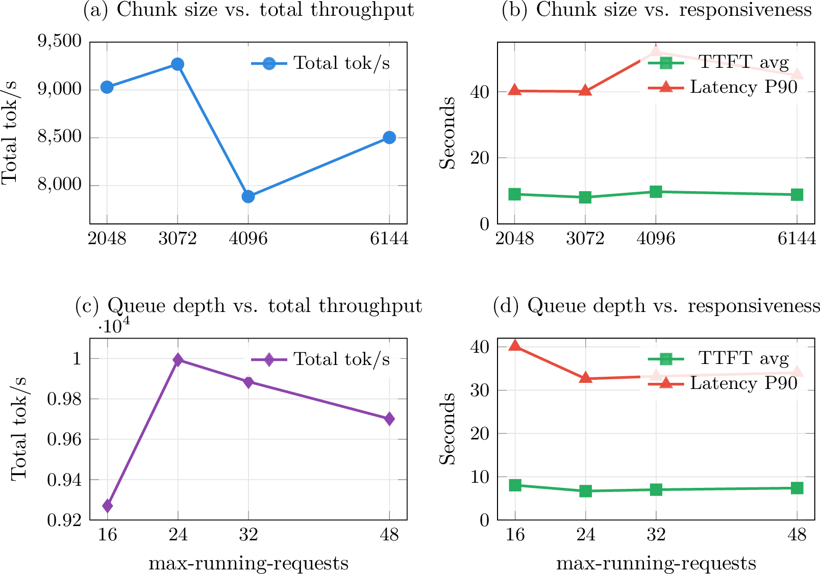
The expanded sweep shows that the best measured point in this workload is chunked-prefill-size=3072, not 4096. Holding tp=4, pp-size=4, and max-running-requests=16 fixed, moving from
2048 to 3072 raises total token throughput from 9029.64 to 9269.88 tok/s and reduces TTFT average from 8.98 to 8.04 seconds, while keeping latency P90 nearly unchanged (40.23 to 40.07 seconds). By contrast, 4096 and 6144 underperform in the max-16 chunk
sweep, with 4096 being the weakest tested chunk size on both throughput and latency. A high-chunk cross-check at 4096/4/4/32 improves over 4096/4/4/16, but it still remains below the recommended 3072/4/4/24 point on
request throughput, total-token throughput, TTFT average, and latency P90.
Interpretation. For the current OpenClaw traffic pattern, 2048 appears slightly too conservative for long-prefix efficiency, while 4096 and above are already large enough to introduce chunk-level burstiness without compensating gains. The sweet spot therefore sits in the middle: 3072 advances long prefills more efficiently than 2048 while avoiding the latency penalty observed at 4096 and 6144 [6].
| Profile | chunk | tp | pp | max-run | Req/s | Total tok/s | Cost / req | Cost / tok | Decision note |
|---|---|---|---|---|---|---|---|---|---|
| Baseline 2048/16 | Rollback point | ||||||||
| Comparison 4096/16 | Not recommended | ||||||||
| Recommended 3072/24 | Default profile |
3pt
5.2 TP/PP Parallelism Ablation↩︎
SGLang supports both tensor parallelism (--tp-size) and pipeline parallelism (--pp-size) [6]. Tensor
parallelism splits intra-layer computation and introduces collective communication; pipeline parallelism splits layers across stages and can suffer stage imbalance and bubble overhead [7], [8]. vLLM documentation similarly notes that distributed serving is highly sensitive to the TP/PP split and interconnect properties [9].
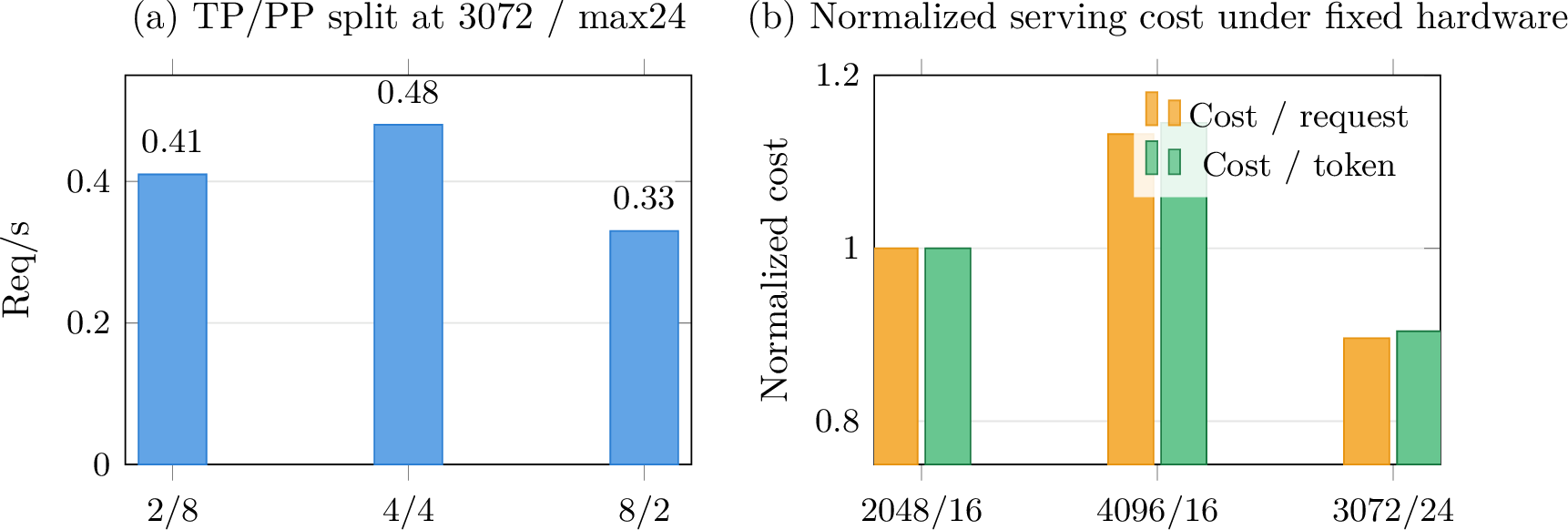
The new data preserve the earlier direction on this axis: tp=4 and pp-size=4 is still the best tested split. Under the same chunked-prefill-size=3072 and max-running-requests=24, the
4/4 split reaches 0.48 req/s and 9993.23 tok/s, compared with 0.41 req/s and 8705.06 tok/s for 2/8, and 0.33 req/s and 6905.99 tok/s for 8/2. TTFT average is also best at 6.69 seconds, versus 7.80 seconds for 2/8 and 9.48 seconds for 8/2.
Interpretation. In this cluster, tp=4 / pp=4 appears to strike the right balance among three competing effects: per-device memory headroom for long-context KV cache, communication cost for TP collectives, and
pipeline balance for PP stages. The 2/8 split likely pays more pipeline bubble cost, while the 8/2 split likely pays more communication and synchronization overhead. As before, this conclusion should be stated conservatively as best among the tested
splits on the current hardware topology [9].
5.3 Max-Running-Requests Ablation↩︎
SGLang’s --max-running-requests caps the number of simultaneously running requests [6]. In many serving setups, raising
this cap increases effective batch size and throughput but eventually worsens queueing delay and tail latency [10].
The best measured point in this sweep is max-running-requests=24, not 16 or 32. Holding chunked-prefill-size=3072, tp=4, and pp-size=4 fixed, moving from 16 to 24 increases request
throughput from 0.44 to 0.48 req/s and total token throughput from 9269.88 to 9993.23 tok/s. At the same time, TTFT average drops from 8.04 to 6.69 seconds and latency P90 drops from 40.07 to 32.64 seconds. Thus, 24 is not merely a higher-throughput mode;
it is a strict improvement over 16 on both efficiency and responsiveness in this workload.
Beyond 24, the gains flatten and then reverse in the 3072 queue sweep. At 32 and 48, throughput remains below the 24-run peak, while TTFT and latency P90 rebound slightly. The separate 4096/4/4/32 cross-check confirms that simply pairing a
larger chunk with deeper queueing does not surpass the 3072/max24 profile. This suggests that the concurrency knee of the current OpenClaw workload sits around 24 running requests. Past that point, queueing and scheduling overhead begin to dominate the
marginal batching benefit.
For this deployment, max-running-requests=24 is the best tested queue-depth setting. It combines the highest measured throughput with the best TTFT and latency P90 among the evaluated alternatives in the current environment [4], [10].
5.3.0.1 Cost reduction under a fixed hardware footprint.
Because all configurations in the current sweep use the same model and the same serving footprint, normalized serving cost can be estimated as the inverse of achieved throughput. On a request basis, \[\mathrm{NormCost}_{\mathrm{req}}(i)=\frac{\mathrm{RPS}_{\mathrm{baseline}}}{\mathrm{RPS}_{i}},\] and on a token basis, \[\mathrm{NormCost}_{\mathrm{tok}}(i)=\frac{\mathrm{TotalTok/s}_{\mathrm{baseline}}}{\mathrm{TotalTok/s}_{i}}.\] Applying these definitions to the measured winner 3072/4/4/24 yields a normalized cost of 0.896 per
request and 0.904 per token, which means a reduction of 10.4% and 9.6% relative to the 2048/4/4/16 baseline. Against the 4096/4/4/16 comparison profile, the savings are even larger: 20.8% per request and 21.1% per token.
6 Conclusions and Recommendations↩︎
Primary conclusion. Within the measured parameter space, the best tested configuration for OpenClaw-serving GLM-5 is:
chunked-prefill-size |
3072 |
tp / pp-size |
4 / 4 |
max-running-requests |
24 |
This profile is the measured winner on both throughput and latency among the tested candidates, rather than a compromise that sacrifices responsiveness for throughput.
Supporting evidence. The measured results indicate: (i) 3072 is a better chunk size than both 2048 and 4096 for this long-context workload, (ii) the queue-depth optimum sits at 24 rather than 16 or 32, and (iii) the 4/4 TP/PP split remains the best tested partitioning choice.
Quantified business impact. Relative to the conservative 2048/4/4/16 baseline, the recommended profile improves request throughput by 11.6% and total token throughput by 10.7%, while reducing TTFT average by 25.5% and
latency P90 by 18.9%. Under constant hardware, this translates into an estimated serving-cost reduction of 10.4% per request and 9.6% per token. Relative to the 4096/4/4/16 comparison profile, the recommended setting reduces normalized serving
cost by roughly 20.8% per request and 21.1% per token.
Operational recommendation. Use 3072 / tp4 / pp4 / max24 as the default OpenClaw profile. Keep 2048 / 4 / 4 / 16 as a conservative rollback point during production rollout if needed. Treat
4096 / 4 / 4 / 16 and TP/PP splits such as 2/8 or 8/2 as not recommended for the current workload, because they are strictly worse on the measured axes.
Further work. A subsequent round should add resource telemetry (GPU utilization, memory headroom, KV-cache occupancy), archive exact benchmark command lines, and repeat the same sweep under several traffic mixes such as pure chat, retrieval-heavy, and tool-heavy sessions. For the present internal deployment decision, the existing measurements are sufficient to nominate the best tested parameter combination and quantify the associated serving-cost reduction; stronger external performance claims should be backed by repeated runs and confidence intervals.