HNSW with Accuracy Guarantees Using Graph Spanners
January 01, 1970
Abstract
Hierarchical Navigable Small World (HNSW) graphs serve as the industry standard due to their logarithmic complexity and strong empirical performance. However, HNSW relies on greedy graph traversal, a heuristic that provides no theoretical guarantees of correctness. In this paper, we propose a novel "Certify-then-Rectify" framework that bridges the gap between the speed of heuristic search and the rigor of exact retrieval. Rather than discarding HNSW, our approach first employs a distribution-free statistical certifier to dynamically evaluate the quality of a standard HNSW search with minimal overhead. If the certification indicates that the retrieved neighbors are of low quality, the framework safely escalates to a rigorous exact recovery algorithm. To make this exact recovery computationally feasible, we reinterpret the HNSW graph as a geometric spanner and utilize Extreme Value Theory to stochastically estimate its maximum empirical stretch factor. This allows us to mathematically bound the maximum distance of true nearest neighbors. Furthermore, we successfully extend these theoretical guarantees to filtered search scenarios. Extensive evaluations on benchmark datasets demonstrate that our tiered framework delivers the average-case speed of HNSW while ensuring the worst-case correctness of exact search.
1 Introduction↩︎
Nearest Neighbor Search (NNS) is the computational engine behind modern AI, driving workloads ranging from Large Language Model (LLM) retrieval to molecular simulations. As datasets scale into the billions of vectors, exact linear scanning becomes computationally prohibitive, necessitating Approximate Nearest Neighbor (ANN) algorithms. Among these, Hierarchical Navigable Small World (HNSW) graphs [1], [2] have become the industry standard due to their logarithmic complexity and generally strong empirical performance.
However, HNSW relies on a greedy traversal of a proximity graph—a heuristic that offers no theoretical guarantee of recall [3]–[6]. While HNSW performs well empirically, it is highly sensitive to hyperparameter selection (e.g., beam width, construction depth) [7], [8]. In high-dimensional spaces, greedy search frequently gets trapped in local minima, failing to retrieve the true nearest neighbor due to topology disconnects or the "curse of dimensionality." While a 95% recall rate is acceptable for e-commerce, it is fundamentally inadequate for logic-driven and scientific domains where a single missing entry can invalidate a result.
The demand for Exact kNN is growing rapidly in complex, high-stakes applications: In training perception models, identifying "hard negatives"—images that look safe but are actually dangerous—is critical [9], [10]. If an ANN algorithm fails to retrieve these specific edge cases during data mining, the training set remains noisy, compromising safety. Exact retrieval is required to rigorously clean training distributions. In systems combining neural retrieval with symbolic logic or LLMs, vector search acts as a predicate selector. Missing a specific "bridge" entity (e.g., a specific legal precedent or protein structure) leads to "hallucinations" or false logical implications because the reasoning engine operates on incomplete premises [11], [12]. Existing attempts to mitigate these failures by simply increasing or predicting [3], [8] HNSW hyperparameters yield diminishing returns, incurring latency penalties without ever providing a guarantee of correctness. Moreover, they impose retraining overheads under distribution shifts.
We propose a novel framework that bridges the gap between the speed of heuristic search and the rigor of exact retrieval. We acknowledge that while our proposed search method, MBV (Metric Bound Verification) (utilizing our proposed Stretch Bounded Expansion from Query), accurately provides a formal probabilistic guarantee, it is computationally slower than heuristic HNSW. Therefore, rather than discarding HNSW, we wrap it in a Certify-then-Rectify (CTR) framework.
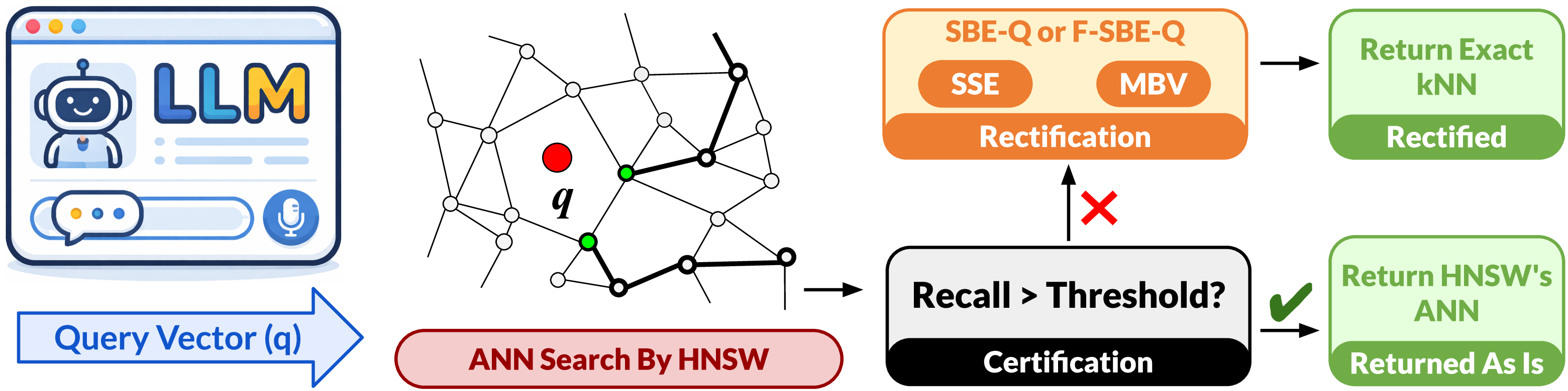
Our approach allows users to first certify the quality of a standard HNSW search result with negligible overhead. If—and only if—the certification indicates that the retrieved neighbors are of low quality, we trigger the computationally heavier MBV algorithm to identify the exact kNN, with high tunable probability 1. This tiered strategy provides the best of both worlds: the average-case speed of HNSW and the worst-case correctness of exact search (see Figure 1). Our implementation is also made publicly available 2.
Our contributions are structured as follows (see Figure 1):
1.0.0.1 1. Stochastic Stretch Estimation (SSE):
To enable exact search, we reinterpret the HNSW graph as a geometric spanner. We introduce SSE, a sampling algorithm that accurately approximates the graph’s stretch factor t. This factor allows us to mathematically bound the maximum distance the true nearest neighbor could reside from our approximate candidates, establishing a dynamic search radius.
1.0.0.2 2. Stretch-Bounded Expansion (SBE-Q):
We present SBE-Q a technique to recover the exact neighbors. Unlike greedy heuristic descent, SBE-Q performs a principled expansion.
SBE from the Query Point (SBE-Q): We confine the search to a radius defined by the distance to the k-th approximate neighbor (\(d_k\)) multiplied by the stretch factor t (i.e., radius=\(t \times d_k\)). This guarantees the discovery of the true nearest neighbors.
Reservoir Sampling: To ensure SBE-Q remains theoretically sound, we use reservoir sampling to virtually "insert" the query point q into the stretch estimation sample without altering the graph’s global stretch properties.
We also explore a baseline variant, SBE-NN (Expansion from Nearest Neighbor), but find SBE-Q significantly more efficient due to its tighter bounding radius.
1.0.0.3 3. Metric Bound Verification (MBV):
Finally, we refine the candidate set obtained by SBE-Q using triangular inequality bounds derived from the stretch factor. This step recycles distance computations from the initial search to strictly filter points, ensuring the final output is the exact k-NN set. Our approach will work for any distance metric that directly or indirectly satisfies triangle inequality.
1.0.0.4 4. Utility in Filtered Search:
We further demonstrate that SBE-Q naturally adapts to filtered search (e.g., "nearest vector where property P is true"), addressing scenarios where filtering fractures the small-world topology. Our techniques can be utilized within extensions like ACORN [2] to prevent traversals from getting stranded in disconnected subgraphs. Theoretical and experimental details are in Section 8. The CTR framework is also fully integrated with DiskANN [13] in the disk-resident graph search setting and experimental details are in Section 7.10.
1.0.0.5 5. Certification of HNSW Results:
We introduce a post-hoc, distribution-free statistical certification framework for vanilla HNSW. By leveraging Conformal Risk Control (CRC) [14], [15] and Learn-then-Test (LTT) [16] procedures, we construct a rigorous certifier that evaluates a distance-margin score derived purely from HNSW’s internal search state. This approach establishes finite-sample statistical guarantees on expected recall shortfall and provides per-query probabilistic bounds. Ultimately, this certifier acts as a dynamic gatekeeper with minimal computational overhead, determining whether to confidently accept the fast heuristic results or to safely escalate to exact recovery via MBV. The entire approach is realized as a lightweight wrapper around existing HNSW implementations, facilitating ease of use.
1.0.0.6 6. End-to-End Guarantee:
We establish a formal end-to-end probabilistic recall guarantee for the complete Certify-then-Rectify framework (Section 6.4).
2 Preliminaries↩︎
In this section, we formalize the problem of Nearest Neighbor Search (NNS) and the structure of Hierarchical Navigable Small World (HNSW) graphs. We establish the notation for the search procedure and its computational artifacts, and we introduce the concept of graph spanners and stretch factors, which form the theoretical basis of our proposed method.
Let \(\mathcal{X}\) be a dataset of \(n\) points in a \(d\)-dimensional vector space equipped with a distance metric \(dist(\cdot, \cdot)\) (typically Euclidean distance). Given a query \(q\) and an integer \(k\), the Exact \(k\)-Nearest Neighbor (\(k\)-NN) problem is to find the set \(\mathcal{N}^*_k(q) \subseteq \mathcal{X}\) such that \(|\mathcal{N}^*_k(q)| = k\) and \(\forall x \in \mathcal{N}^*_k(q), \forall y \in \mathcal{X} \setminus \mathcal{N}^*_k(q), dist(q, x) \leq dist(q, y)\).
The HNSW index is a hierarchical graph structure approximating the proximity of points in \(\mathcal{X}\). It consists of a series of layers \(L_0, L_1, \dots, L_{l_{max}}\), where layer \(L_0\) contains all data points, and each subsequent layer \(L_i\) contains a subset of the points from layer \(L_{i-1}\), forming a hierarchy. Formally, an HNSW structure is a tuple of graphs \(\mathcal{H} = (G_0, G_1, \dots, G_{l_{max}})\). Each graph \(G_i = (V_i, E_i)\) is defined such that \(V_i \subseteq \mathcal{X}\). The edges \(E_i\) connect points within the same layer based on proximity heuristics. The hierarchy allows for logarithmic search complexity by initiating the search at the top layer (coarse granularity) and progressively refining the search region as traversal moves down to layer \(L_0\) (fine granularity).
Construction proceeds iteratively by inserting points \(x \in \mathcal{X}\). For each \(x\), a maximum layer \(l(x) \leq l_{max}\) is selected randomly based on an exponential distribution. The point is inserted into all graphs \(G_0, G_1, \dots, G_{l(x)}\). Connections in each layer are established using a heuristic selection strategy that balances proximity with spatial diversity (connectivity) to ensure the "small world" property, typically bounded by a maximum degree parameter \(M\).
The search for the \(k\)-NN of a query \(q\) in HNSW is a greedy traversal. Starting from an entry point \(e_{top}\) in the top layer \(L_{l_{max}}\), the algorithm greedily moves to the neighbor minimizing \(dist(q, \cdot)\) until a local minimum is reached. This process repeats down to layer \(L_0\). In layer \(L_0\), a beam search is conducted with a beam width parameter \(ef\). Let this process be denoted as \(\text{Search}(q, k, ef)\). The output of this heuristic search is an approximate set \(\mathcal{N}_k(q) \subseteq \mathcal{X}\), where often \(|\mathcal{N}_k(q)| < k\) and \(\mathcal{N}_k(q) \cap \mathcal{N}^*_k(q)\) may be empty in worst-case scenarios. Crucially, our approach utilizes the artifacts generated during this traversal. We define the Search Trace \(\mathcal{T}(q)\) as the set of all points for which the distance to \(q\) was computed during the search: \[\mathcal{T}(q) = \{ x \in \mathcal{X} \mid dist(q, x) \text{ was computed during } \text{Search}(q, k, ef) \}.\] This set includes the visited nodes and their immediate neighbors evaluated during the beam search. To bound the error of the approximate search, we analyze the bottom-layer graph \(G_0\) as a geometric spanner.
Definition 1. A weighted graph \(G = (V, E)\), where vertices are points in a metric space \((\mathcal{X}, dist)\), is a \(t\)-spanner if, for every pair of vertices \(u, v \in V\), the shortest path distance in the graph, denoted \(d_G(u, v)\), satisfies: \[dist(u, v) \leq d_G(u, v) \leq t \cdot dist(u, v).\] The value \(t \geq 1\) is called the stretch factor (or dilation) of the spanner.
In the context of NNS, the stretch factor limits how much the graph topology distorts the true metric space. If \(G_0\) were a perfect 1-spanner (a complete graph with edge weights equal to metric distances), greedy search would be exact. The sparsification required for efficiency introduces distortion. While HNSW construction heuristics do not theoretically guarantee a constant stretch factor \(t\) for arbitrary worst-case inputs (i.e., it is not a \(t\)-spanner by design in the traditional computational geometry sense), any realized finite HNSW graph instance \(G_0\) possesses an intrinsic, maximum empirical stretch \(t_{emp}\) defined as: \[t_{emp} = \max_{u, v \in \mathcal{X}} \frac{d_{G_0}(u, v)}{dist(u, v)}.\] This property is pivotal: if we know (or estimate) \(t_{emp}\), we can relate the graph distance—which we can explore efficiently via Breadth-First Search (BFS) or Dijkstra—to the unknown metric distance \(dist(q, x)\), thereby establishing a stopping condition for search expansion that guarantees the inclusion of \(\mathcal{N}^*_k(q)\).
3 STOCHASTIC STRETCH ESTIMATION↩︎
For graphs of realistic sizes, computing the stretch factor exactly is not computationally feasible, as it would involve computations quadratic to the number of nodes in the graph. We, in turn, present sampling based algorithms to estimate the stretch factor of an HNSW graph \(G\).
Let \(S\) be a random variable representing the stretch factor of a uniformly random pair \((u,v)\) from \(V \times V \setminus \{(v,v) : v \in V\}\). Rather than estimating arbitrary percentiles, our goal is to estimate the absolute maximum empirical stretch factor via a finite sample.
Definition 2 (Sample Block Maxima). Let the total sampled pairs be divided into \(m\) blocks of size \(n\). Let \(M_{n,i} = \max\{S_{i,1}, \dots, S_{i,n}\}\) be the maximum stretch factor observed in the \(i\)-th block.
Theorem 1 (EVT Maximum Stretch Bound). According to the Fisher-Tippett-Gnedenko theorem [17], the distribution of the maximum of a large sequence of independent, identically distributed random variables converges to a specific family of distributions. For the right tail of the stretch factor distribution, the cumulative distribution function (CDF) of the block maxima converges to the Generalized Extreme Value (GEV) distribution: \[H(s; \mu, \sigma, \xi) = \exp\left(-\left[1 + \xi\left(\frac{s-\mu}{\sigma}\right)\right]^{-1/\xi}\right)\] where \(\mu\) is the location parameter, \(\sigma > 0\) is the scale parameter, and \(\xi\) is the shape parameter.
By modeling the “right tail” (the largest observed stretch factors) of our sample, we can accurately estimate the unobserved probability density of extreme stretch distortions. For a given confidence level \(\beta \in (0,1)\), the estimated maximum stretch factor \(t^*\) is defined as the return level derived from the inverse CDF of the fitted GEV distribution: \[t^* = \mu - \frac{\sigma}{\xi} \left[ 1 - (-\ln \beta)^{-\xi} \right]\]
Thus, with confidence \(\beta\), the true empirical stretch factor of the graph is bounded by \(t^*\).
3.1 Practical Application of the EVT Bound↩︎
In practice, applying Theorem 3.2 requires a systematic sampling and fitting procedure prior to initiating the search. First, we generate a large pool of independent stretch factor samples by computing the exact metric distance and the shortest-path graph distance for random pairs of vertices in \(G\). This pool is then partitioned into \(m\) distinct blocks of size \(n\). We extract the maximum stretch value from each block, resulting in a specialized dataset composed entirely of block maxima. Next, we apply Maximum Likelihood Estimation (MLE) to this dataset to find the optimal parameters for the Generalized Extreme Value distribution: the location \(\mu\), scale \(\sigma\), and shape \(\xi\). Once the MLE converges and the parameters are established, we substitute them—along with our target confidence level \(\beta\) (e.g., \(0.99\))—into the GEV return level equation. The resulting value, \(t\), acts as the rigorously defined operating stretch factor for our subsequent search expansions, ensuring the search radius dynamically adapts to the graph’s most extreme topological distortions.
4 Graph based pruning techniques↩︎
4.1 Stretch Bounded Expansion from Nearest Neighbor (SBE-NN)↩︎
We consider \((\mathcal{X}, \mathit{dist})\) to be a metric space, where \(G_0=(\mathcal{X},E)\) corresponds to the bottom-layer HNSW graph. Notably, this can be viewed as a weighted graph where each edge \((u,v)\in E\) has weight \(\mathit{dist}(u,v)\). We denote the shortest-path distance in \(G_0\) (sum of edge weights) as \(d_{G_0}(u,v)\).
Assuming \(G_0\) to be a \(t\)-spanner (globally or locally in the vicinity of \(q\)) in the sense that for all relevant pairs \(u,v\): \[\mathit{dist}(u,v) \le d_{G_0}(u,v) \le t \cdot \mathit{dist}(u,v)\]
To analyze the search expansion, we must distinguish between the approximate candidates returned by the HNSW index and the unknown ground truth.
For a given query \(q\), let the ordered set of \(k\) candidates returned by the initial HNSW search be \(\{x_{(1)}, x_{(2)}, \dots, x_{(k)}\}\). We define the distances to the nearest and \(k\)-th candidates as: \[\hat{d}_1 = \mathit{dist}(q, x_{(1)}) \quad \text{and} \quad \hat{d}_k = \mathit{dist}(q, x_{(k)})\]
Let \(N_k^*(q)\) denote the set of the true top-\(k\) nearest neighbors. Let \(d_k^*\) denote the distance to the true \(k\)-th nearest neighbor: \[d_k^* = \max_{x \in N_k^*(q)} \mathit{dist}(q, x)\]
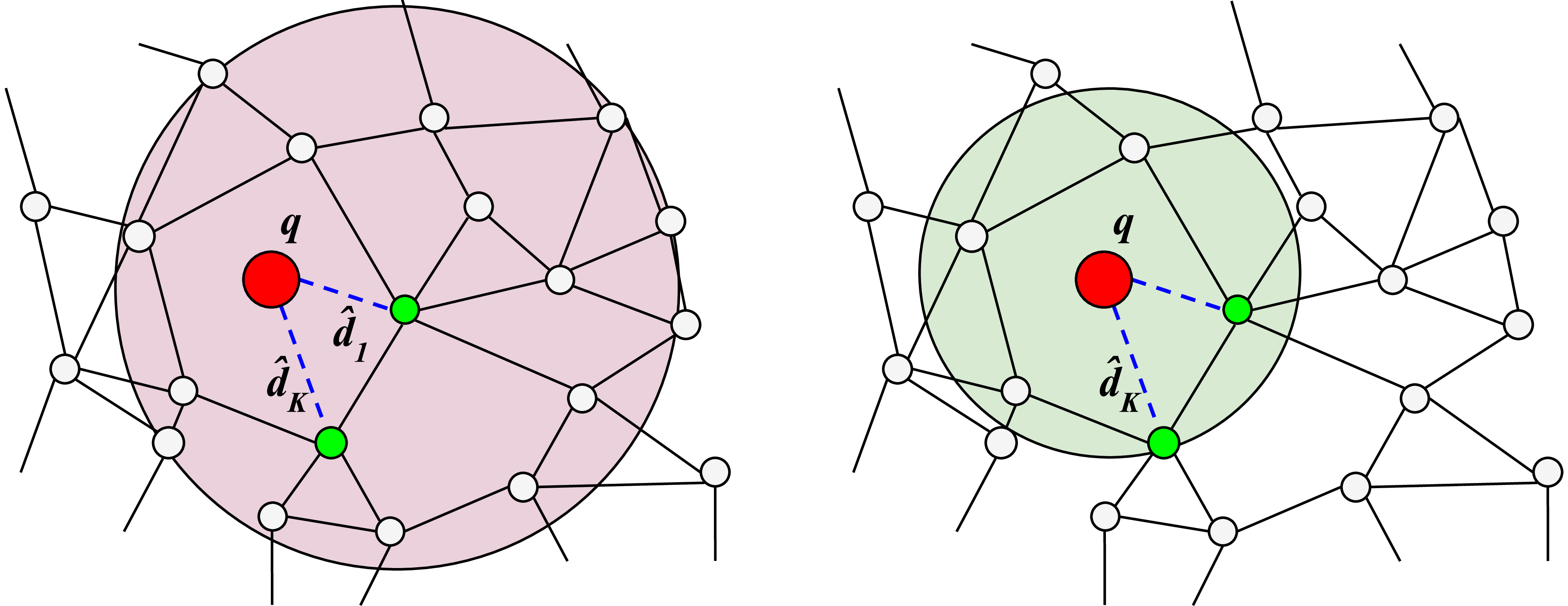
Since the HNSW candidates \(\{x_{(1)}, \dots, x_{(k)}\}\) form a valid subset of \(\mathcal{X}\) of size \(k\), and the true set \(N_k^*(q)\) minimizes the sum of distances, it necessarily holds that the true \(k\)-th distance is bounded by the approximate \(k\)-th distance: \[\label{eq:bound95dk} d_k^* \le \hat{d}_k\tag{1}\] This observation allows us to construct a search radius based on the observed HNSW results that guarantees the inclusion of the unknown true neighbors as per Figure 2.
Theorem 2 (Stretch-bounded containment of true top-k). Given a query \(q\), let \(x_{(1)}\) be the nearest candidate and \(\hat{d}_k\) be the distance to the \(k\)-th candidate returned by HNSW. Every point in the true top-\(k\) set \(N_k^*(q)\) lies inside the graph ball of radius \(t(\hat{d}_1 + \hat{d}_k)\) centered at \(x_{(1)}\).
Formally, for every \(x^* \in N_k^*(q)\): \[d_{G_0}(x_{(1)}, x^*) \le t(\hat{d}_1 + \hat{d}_k)\] Consequently: \[N_k^*(q) \subseteq \{x \in \mathcal{X} : d_{G_0}(x_{(1)}, x) \le t(\hat{d}_1 + \hat{d}_k)\}\]
Proof. Let \(x^*\) be any point in the true set \(N_k^*(q)\). By definition of the true \(k\)-th distance and Equation 1 : \[\label{eq:one} \mathit{dist}(q, x^*) \le d_k^* \le \hat{d}_k\tag{2}\]
Using the triangle inequality in the metric space: \[\label{eq:two} \mathit{dist}(x_{(1)}, x^*) \le \mathit{dist}(x_{(1)}, q) + \mathit{dist}(q, x^*)\tag{3}\] Substituting known variables \(\mathit{dist}(x_{(1)}, q) = \hat{d}_1\) and the bound from Equation 2 : \[\mathit{dist}(x_{(1)}, x^*) \le \hat{d}_1 + \hat{d}_k\] This represents the maximum possible metric distance between the entry point \(x_{(1)}\) and any true answer \(x^*\). This worst-case occurs when \(q\) lies strictly between \(x_{(1)}\) and \(x^*\) (collinear).
Since \(G_0\) is a \(t\)-spanner, the graph distance is bounded by \(t\) times the metric distance: \[\label{eq:three} d_{G_0}(x_{(1)}, x^*) \le t \cdot \mathit{dist}(x_{(1)}, x^*)\tag{4}\] Combining these inequalities yields: \[\label{eq:four} d_{G_0}(x_{(1)}, x^*) \le t(\hat{d}_1 + \hat{d}_k)\tag{5}\] As \(x^*\) was arbitrary, the inclusion holds for all true top-\(k\) points. ◻
Figure 2 (left) illustrates Dijkstra’s search region as the ball with radius \(t\cdot(\hat{d}_1+\hat{d}_k)\) centered at the first nearest neighbor. Any embedded vector outside of the ball is pruned.
4.2 Stretch Bounded Expansion from Query (SBE-Q)↩︎
While SBE-NN (Section 4.1) guarantees exactness, the search radius relies on the triangle inequality to bridge the gap between the starting node \(x_{(1)}\) and the query \(q\). This introduces unnecessary “slack” in the search bound—specifically the term \(\hat{d}_1 = \mathit{dist}(x_{(1)}, q)\). In high-dimensional spaces, even the nearest neighbor may be at a significant distance from \(q\), inflating the search radius unnecessarily. To tighten this bound, we propose SBE-Q, which conceptually initiates the expansion directly from the query point \(q\).
To formalize this, we treat the query \(q\) as a temporary node inserted into the graph \(G\). Let \(G' = (V', E')\) denote the graph augmented with \(q\), where \(V' = V \cup \{q\}\). Edges are established between \(q\) and the top-\(M_0\) computed candidates to respect graph degree upper bound. (In the case \(k<M_0\), we use \(k\).) This virtual insertion alters the graph topology. In Section 4.3, we demonstrate how to efficiently test the stretch factor of \(G'\). Let \(t'\) be the stretch factor of the augmented graph \(G'\) (which may differ from \(t\)). We derive a bound depending solely on \(\hat{d}_k\) and \(t'\), eliminating the \(\hat{d}_1\) overhead (see Figure 2).
Theorem 3 (Stretch-Bounded Expansion from Query). Let \(q\) be a query point virtually inserted into the graph \(G\) such that the augmented graph \(G'\) is a \(t'\)-spanner. Let \(\hat{d}_k\) be the distance to the \(k\)-th candidate returned by HNSW. Every true top-\(k\) point lies inside the graph ball of radius \(t' \cdot \hat{d}_k\) centered at \(q\).
Formally, for every \(x^* \in N_k^*(q)\): \[\label{eq:sbe-q-bound} d_{G'}(q, x^*) \le t' \cdot \hat{d}_k\tag{6}\]
Proof. Let \(x^*\) be any arbitrary point in the true \(k\)-nearest neighbor set \(N_k^*(q)\). By definition of the true set and the property that the HNSW \(k\)-th distance is an upper bound (\(d_k^* \le \hat{d}_k\)): \[\label{eq:metric-bound} \mathit{dist}(q, x^*) \le d_k^* \le \hat{d}_k\tag{7}\]
Since the augmented graph \(G'\) satisfies the \(t'\)-spanner property for the pair \((q, x^*)\), the shortest path distance in \(G'\) is bounded by the metric distance scaled by \(t'\): \[\label{eq:spanner-bound} d_{G'}(q, x^*) \le t' \cdot \mathit{dist}(q, x^*)\tag{8}\]
Combining Inequality 7 and Inequality 8 , we obtain: \[d_{G'}(q, x^*) \le t' \cdot \hat{d}_k\]
Since this holds for any arbitrary \(x^* \in N_k^*(q)\), the entire set of true nearest neighbors is contained within the graph ball \(B_{G'}(q, t' \cdot \hat{d}_k)\). ◻
Remark 1. The SBE-Q bound \(d_{G'}(q, x) \le t' \cdot \hat{d}_k\) is strictly tighter than the SBE-NN bound \(d_{G_0}(x_{(1)}, x) \le t (\hat{d}_k + \hat{d}_1)\) whenever \(t' \approx t\). By shifting the expansion center to \(q\), we remove the penalty \(\hat{d}_1\) (the distance from the query to the closest returned candidate). In Section 7.4, we empirically demonstrate that this approach significantly reduces the volume of the graph explored while maintaining probabilistic guarantees.
Figure 2 (right) illustrates Dijkstra’s search region as the ball with radius \(t\cdot \hat{d}_k\) centered at the query point \(q\). The Dijkstra’s expansion is smaller than the expansion obtained by starting the search at the first nearest neighbor (left panel), because we do not need to traverse the additional \(t\cdot \hat{d}_1\) term again.
4.3 Incremental Stretch Factor Estimation↩︎
For an HNSW graph \(G=(V,E)\) of realistic size, re-evaluating the stretch factor distribution from scratch after every “virtual” query insertion is computationally prohibitive. We seek to maintain the validity of the EVT bounds derived in Section 3 without incurring the cost of a full resample.
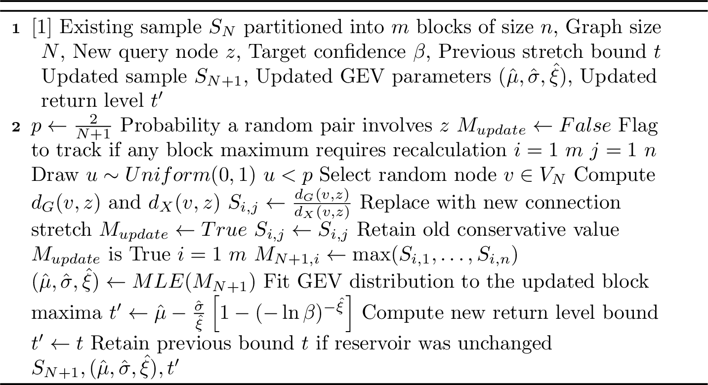
When we simulate the insertion of a query node \(q\), the population of vertex pairs expands. To maintain a representative sample of tail extremes without full re-computation, we employ a reservoir-style update that probabilistically injects new pairs involving \(q\) while retaining existing sample values.
4.3.0.1 Algorithm: Incremental Reservoir Tail Patching.
Because the insertion of \(q\) adds edges to the graph, the shortest path distance \(d_G(u,v)\) for any existing pair \((u,v)\) can only decrease or remain constant; it cannot increase. Therefore, the previously sampled extreme stretch values either remain accurate or act as conservative overestimates. We define the update probability \(p\) as the likelihood that a uniformly random pair in the augmented graph involves the new node \(q\). If a newly sampled stretch factor involving \(q\) falls into the extreme right tail, it is injected into the pool of block maxima, and the GEV parameters \((\mu,\sigma,\xi)\) are efficiently refitted. Algorithm 3 presents the overall approach.
4.3.1 Theoretical Guarantees↩︎
We assert that the sample of extreme values updated by the Incremental Reservoir Tail Patching algorithm allows for a valid certification of the maximum stretch factor using the methodology of Theorem 1.
Theorem 4 (Conservative EVT Certification). Let \(S_{ext}\) be the pool of extreme stretch values maintained during incremental insertion. Let \((\hat{\mu}, \hat{\sigma}, \hat{\xi})\) be the GEV parameters fitted to \(S_{ext}\). For a confidence level \(\beta\), the probability that the true maximum stretch factor of the augmented graph \(G'\) does not exceed the estimated return level \(t'\) is at least \(\beta\).
Proof. The validity of this bound relies on the monotonically non-increasing nature of graph distances under edge addition. For retained pairs not involving \(q\), the stored stretch value \(S^{old}\) satisfies \(S^{old} \ge S^{true}\). Therefore, the right tail of our sampled distribution stochastically dominates the true right tail of the augmented graph. Fitting the GEV distribution to these conservative maxima yields a return level \(t'\) that safely upper-bounds the true maximum stretch. ◻
4.3.2 Complexity Analysis↩︎
The computational efficiency of this incremental strategy is superior to full resampling. The number of distance computations required follows a Binomial distribution \(K \sim B(n,p)\), where \(p = \frac{2}{N+1}\). The expected number of computations is \(E[K] = \frac{2n}{N+1}\).
For a typical configuration where the graph size \(N\) is large, the expected graph distance sampling cost is negligible. The primary additional overhead is the Maximum Likelihood Estimation (MLE) required to update the three GEV parameters \((\mu, \sigma, \xi)\). Because MLE is performed solely on the small subset of extreme tail values rather than the entire sample, it operates in \(\mathcal{O}(m)\) time (where \(m\) is the number of block maxima), effectively allowing for continuous certification with near-zero marginal cost per simulated insertion.
5 Metric Bound Verification↩︎
While the Stretch-Bounded Expansion (SBE-Q and F-SBE-Q) described in Sections 4.2 and 8 provides a theoretical containment guarantee for the true \(k\)-nearest neighbors, naively evaluating the metric distance \(dist(q, v)\) for every node \(v\) within the search radius \(t' \cdot d_k\) can be computationally expensive. To bridge the gap between theoretical exactness and practical latency, we introduce Metric Bound Verification (MBV).
MBV is a pruning mechanism integrated directly into the graph traversal. It exploits the triangular inequality inherent in the metric space to discard candidates within the search radius without performing explicit distance computations. By maintaining recursive lower bounds on the distance from the query to the current node, we can rigorously certify that specific sub-branches of the graph cannot contain better candidates than those already found.
These pruning mechanisms are universal; they apply equally to the unconstrained SBE-Q search and the filtered F-SBE-Q search, as they rely solely on metric space properties independent of node attributes.
5.1 Recursive Lower Bound Pruning↩︎
The core of MBV relies on propagating lower bounds down the search tree (the path taken by Dijkstra’s algorithm from the virtual query node \(q\)). For any node \(u\) visited during the expansion, let \(p\) be its parent in the search trace (i.e., the node that added \(u\) to the priority queue). By the triangle inequality, the metric distance \(\mathit{dist}(q, u)\) is lower-bounded by the distance to the parent minus the edge weight connecting them: \[\mathit{dist}(q, u) \ge \mathit{dist}(q, p) - \mathit{dist}(p, u)\] Since the edge weight \(w(p, u)\) in the graph corresponds to the metric distance between \(p\) and \(u\), we can derive a recursive lower bound \(LB(u)\). This bound depends on whether the parent \(p\) was fully evaluated or merely pruned (where only a lower bound is known).
Evaluated Parent: If \(\mathit{dist}(q, p)\) has been computed (note if this distance was in the Search Trace \(\mathcal{T}(q)\), as per section 2, it will be re-used), then: \(LB(u) = \mathit{dist}(q, p) - w(p, u)\)
Pruned Parent: If \(p\) was pruned based on its own lower bound \(LB(p)\), we propagate the uncertainty: \(LB(u) = LB(p) - w(p, u)\)
Let \(\hat{d}_k\) be the distance to the current \(k\)-th nearest neighbor found so far (initially from HNSW, then updated dynamically). If \(LB(u) >
\hat{d}_k\), we can certify that \(u\) is strictly worse than the current candidate set and cannot improve the result. Consequently, we mark \(u\) as PRUNED and skip the
expensive \(\mathit{dist}(q, u)\) calculation (Figure 4). Crucially, we still explore \(u\)’s neighbors, as the graph topology may lead back toward \(q\), but we do so carrying the derived lower bound.

5.2 Elliptical Search Space Pruning↩︎
Beyond avoiding distance computations, we can also prune the search space itself using an “Elliptical Intersection” check. If the exact distance \(\mathit{dist}(q, u)\) is computed, we can determine if the entire branch stemming from \(u\) is effectively dead. A node \(u\) can be discarded—preventing the addition of its neighbors to the queue—if the path through \(u\) cannot possibly reach a point closer than the current \(k\)-th neighbor bound \(\hat{d}_k\) within the remaining search budget.
Formally, if \(d_{G'}(q, u)\) is the graph distance traveled so far and \(R_{search} = t' \cdot \hat{d}_k\) is the current stretch-bounded radius, any descendant \(v\) must satisfy \(d_{G'}(q, v) \le R_{search}\). This implies the “remaining fuel” from \(u\) is \(R_{search} - d_{G'}(q, u)\). If the metric distance \(\mathit{dist}(q, u)\) exceeds this remaining capacity plus the target distance \(\hat{d}_k\), no descendant can qualify. The pruning condition is (Figure 4): \[\label{eq:ellipse-pruning} d_{G'}(q, u) + \mathit{dist}(q, u) > t' \cdot \hat{d}_k + \hat{d}_k\tag{9}\] This check tightens the search region from a simple graph ball to the intersection of the graph ball and the underlying metric constraints.
5.3 Algorithm↩︎
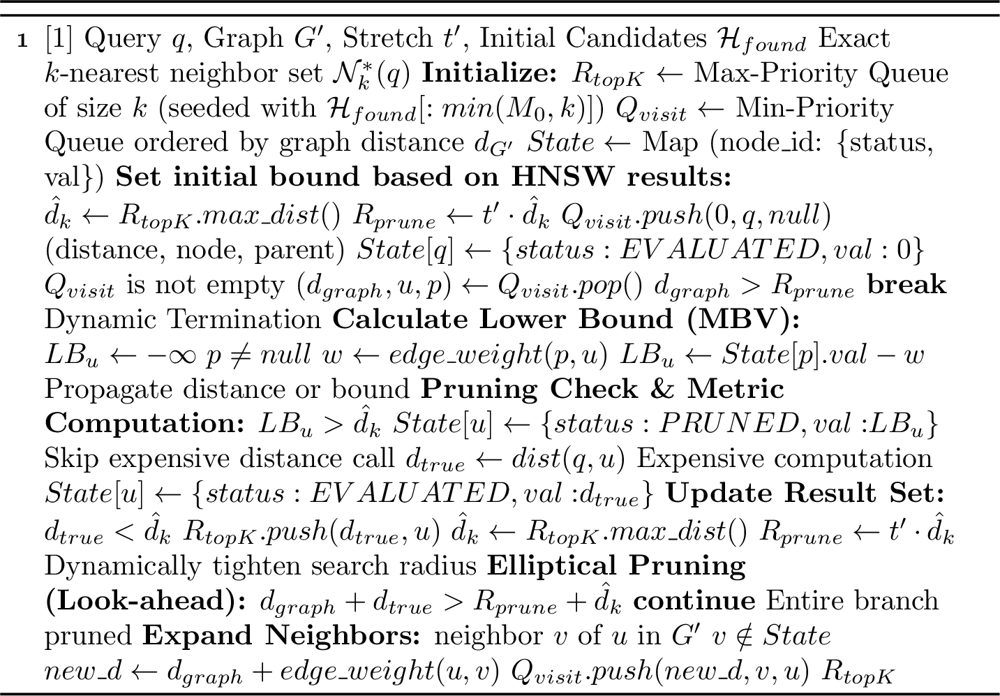
The integrated procedure, SBE-Q with Metric Bound Verification, is detailed in Algorithm 5. It replaces the naive expansion phases, ensuring that expensive metric evaluations are minimized while maintaining the probabilistic guarantees of exactness derived in Theorem 3.
This algorithm upgrades the heuristic search of an HNSW graph into an exact retrieval engine by rigorously bounding the search space and pruning unnecessary calculations. It operates through two integrated mechanisms:
5.3.0.1 Stretch-Bounded Expansion (SBE):
The search treats the query \(q\) as a virtual node and expands strictly within a dynamic radius \(R_{\text{prune}} = t' \cdot \hat{d}_k\). This radius is derived from the graph’s stretch factor \(t'\) and the current best-known \(k\)-th distance \(\hat{d}_k\). Since the true \(k\)-th distance \(d_k^*\) satisfies \(d_k^* \le \hat{d}_k\), this radius guarantees that all true \(k\)-nearest neighbors are contained within the boundary. As better candidates are discovered, \(\hat{d}_k\) decreases, automatically shrinking the search radius. Specifically:
- Discovery of Better Candidates:
-
As the expansion traverses the graph, it computes the exact metric distance \(d_{true}\) for a visited node \(u\). If \(d_{true} < \hat{d}_k\), \(u\) improves upon the current top-\(k\) set.
- The Update Event:
-
The algorithm inserts \(u\) into the priority queue of results (\(R_{topK}\)) and removes the previous furthest candidate. Consequently, \(\hat{d}_k\) immediately decreases.
- Tightening the Radius:
-
This reduction in \(\hat{d}_k\) triggers an immediate recalculation of \(R_{prune} = t' \cdot \hat{d}_k\). The algorithm effectively “pulls in” the search horizon, pruning pending nodes in the queue that are now outside the new, tighter boundary.
5.3.0.2 Metric Bound Verification (MBV):
To avoid expensive metric distance computations for every visited node, the algorithm applies two pruning checks:
Recursive Lower Bound Pruning: It utilizes the triangle inequality to propagate lower bounds from parent nodes to their children. If a node’s lower bound distance \(LB(u)\) exceeds the current \(\hat{d}_k\), the node is discarded without performing the expensive distance calculation.
Elliptical Pruning: It evaluates if a graph branch is “dead” by checking if the path through a node can possibly reach a better candidate within the remaining search budget. If \(d_{G'}(q, u) + \mathit{dist}(q, u) > (t' + 1) \cdot \hat{d}_k\), the entire branch is pruned.
Together, these techniques guarantee the retrieval of the exact \(k\)-nearest neighbors while maintaining efficiency by aggressively filtering out unpromising candidates. Figure 4 (right) presents the Elliptical Search Space Pruning technique where the node \(u\) is far enough from \(q\) by graph distance (path shown in blue), such that any descendant of \(u\) (shown by the red cloud) in the shortest-path tree will not be within the top-k as they are far away in vector space as well (shown by the orange line) and thus, can be pruned.
6 Statistical Certification via Conformal Risk Control↩︎
We frame the “Certify” phase of our “Certify-then-Rectify” workflow as a distribution-free selective prediction problem. By leveraging Conformal Risk Control (CRC) [14], [15] and Learn-then-Test (LTT) [16] procedures, we construct a rigorous statistical certifier. This certifier acts as a gatekeeper, dynamically deciding whether to trust the fast, approximate candidates returned by HNSW, or to escalate to the exact, but computationally heavier, exact recovery procedures (SBE-Q and MBV).
6.1 Problem Setup and Certifiability Score↩︎
Let \(\mathcal{N}_{k}(q)\) represent the approximate top-\(k\) candidates returned by the vanilla HNSW greedy traversal. Let \(\mathcal{N}_{k}^{*}(q)\) represent the true \(k\)-nearest neighbors obtained via an exact oracle (in our framework, this oracle is SBE-Q coupled with MBV). We define the per-query recall as: \[Recall(q) = \frac{|\mathcal{N}_{k}(q) \cap \mathcal{N}_{k}^{*}(q)|}{k}\]
Given a target recall threshold \(\tau \in (0,1]\), we call a top-\(k\) result set "compliant" to \(\tau\) if \(Recall(q) \ge \tau\). Given \(\tau\) and a target risk level \(\alpha \in (0,1)\), our goal is to build a certifier \(C(q)\) that outputs “accept” only when it can statistically guarantee that the top-\(k\) result set is compliant with \(\tau\).
To achieve this, we define a score \(s(q)\) from HNSW’s internal search trace. We use a compact feature vector \(z(q)\) that captures (i) distance geometry, (ii) search reach, and (iii) path stability: \[\begin{align} z(q)=\Big[\hat{d}_1,\ldots\hat{d}_{100},\;\tilde{d}_1,\ldots,\tilde{d}_{10},|\mathcal{T}(q)|,\;n_{\mathrm{rev}}(q),\;\Delta_{\mathrm{rev}}(q)\Big]. \end{align}\] \(\hat{d}_1,\ldots,\hat{d}_{100}\) are the top-100 returned distances, and in the case \(k<100\), we pad with 0 entries. \(\tilde{d}_1,\ldots,\tilde{d}_{10}\) are the remaining top-10 candidate-frontier distances at termination. These features capture distance geometry. Following previous work [18], we capture the search reach with \(|\mathcal{T}(q)|\), where \(\mathcal{T}(q)\) is the search trace defined in Section 2. We use distance-reversal statistics for path stability: \(n_{\mathrm{rev}}(q)\) is the number of direction reversals in successive expansion distances, and \(\Delta_{\mathrm{rev}}(q)\) is their cumulative magnitude. More precisely, let \[d^{\mathrm{pop}}_1,d^{\mathrm{pop}}_2,\ldots,d^{\mathrm{pop}}_T\] denote the sequence of metric distances from \(q\) of the nodes popped from the bottom-layer HNSW candidate queue. A distance reversal occurs at index \(j\in\{2,\ldots,T-1\}\) whenever the local direction of this sequence changes, i.e., \[\bigl(d^{\mathrm{pop}}_j-d^{\mathrm{pop}}_{j-1}\bigr)\bigl(d^{\mathrm{pop}}_{j+1}-d^{\mathrm{pop}}_j\bigr)<0.\] Equivalently, the popped distances are locally non-monotone; for example, \(100,50,120\) and \(50,120,80\) each contain a reversal. Let \(r_j(q)\) indicate whether a local reversal occurs at position \(j\). We define \(n_{\mathrm{rev}}(q)=\sum_{j=2}^{T-1} r_j(q)\) as the number of reversals, and \(\Delta_{\mathrm{rev}}(q)\) as the sum of the adjacent jump magnitudes (ie. the two factors of the product in the above equation) over all positions \(j\) with \(r_j(q)=1\). These features quantify instability in the HNSW traversal order: larger values indicate that the search path is less geometrically consistent. Our feature-ablation results indicate that distance geometry contributes most of the score separability, while path stability statistics provide complementary gains in harder regimes: removing distance features reduces AUROC by \(0.009\!\sim\!0.055\) across datasets. Removing reversal features has a smaller average effect but still non-negligible (up to \(\Delta\)AUROC \(=0.017\)). This supports using the full vector for cross-dataset robustness. The feature vector is then mapped through logistic regression trained on a calibration set. Crucially, the statistical guarantee is independent of the model’s predictive quality; a poor fit simply yields a more conservative certifier.
6.2 Guaranteeing Expected Shortfall via CRC↩︎
To guarantee the average quality of the certified results without making underlying distributional assumptions about the metric space, we utilize the Conformal Risk Control (CRC) framework. We define the recall shortfall as our per-query loss function: \[l(q) = \max(0, \tau - Recall(q))\]
Given a calibration set \(\mathcal{D}_{cal} = \{(q_{i}, \mathcal{N}_{k}^{*}(q_{i}))\}_{i=1}^{n}\) drawn i.i.d. from an unknown query distribution \(\mathcal{P}\), the procedure operates as follows:
Compute the score \(s_{i} = s(q_{i})\) and the loss \(l_{i}\) for each calibration query, sorting them in descending order of their score.
For any candidate threshold \(\theta\), define the empirical risk as: \[\hat{R}(\theta) = \frac{\sum_{i=1}^{n} l_{i} \cdot \mathbb{1}[s_{i} \ge \theta]}{\sum_{i=1}^{n} \mathbb{1}[s_{i} \ge \theta] + 1}\]
Select the optimal threshold \(\hat{\theta}\) that bounds this empirical risk: \[\hat{\theta} = \inf \left\{ \theta : \hat{R}(\theta) \le \alpha(1-\tau) \cdot \frac{n}{n+1} \right\}\]
Theorem 6.1 (CRC Guarantee for HNSW Recall). If the calibration queries \(q_1, ..., q_n\) are i.i.d. from \(\mathcal{P}\), then for a new test query \(Q \sim \mathcal{P}\), the certifier \(C(Q) = \mathbb{1}[s(Q) \ge \hat{\theta}]\) satisfies: \[\mathbb{E}[l(Q) \cdot \mathbb{1}[s(Q) \ge \hat{\theta}]] \le \alpha(1-\tau)\] This guarantee is exact in a finite-sample sense and requires no knowledge of HNSW’s internal workings.
6.3 Pointwise Guarantees via Learn-then-Test (LTT)↩︎
If a strict, per-query probabilistic guarantee is required, we deploy the Learn-then-Test (LTT) framework. LTT controls the certifier’s precision, ensuring that \(\mathbb{P}_{q \sim \mathcal{P}}[Recall(q) \ge \tau \mid s(q) \ge \hat{\theta}] \ge 1 - \epsilon\) with a confidence level of \(1 - \alpha\).
We split the calibration set \(\mathcal{D}_{cal}\) into a training set \(\mathcal{D}_{tr}\) and a test set \(\mathcal{D}_{te}\). From \(\mathcal{D}_{tr}\), we define a finite set of candidate thresholds \(\Theta\). For each candidate threshold \(\theta \in \Theta\) evaluated on \(\mathcal{D}_{te}\), we test the null hypothesis \(H_{0}^{\theta} : \mathbb{P}[Recall(q) < \tau \mid s(q) \ge \theta] > \epsilon\).
Let \(m_{\theta}\) denote the number of certified queries and \(x_{\theta}\) denote the subset of those queries that failed to meet the target recall. We compute the one-sided binomial p-value: \[\text{p-value} = \sum_{j=0}^{x_{\theta}} \binom{m_{\theta}}{j} \epsilon^{j}(1-\epsilon)^{m_{\theta}-j}\] To account for multiple testing over \(\Theta\), we apply a Bonferroni correction, rejecting \(H_{0}^{\theta}\) only if \(\text{p-value} \le \frac{\alpha}{|\Theta|}\). The final threshold is selected as: \[\hat{\theta} = \max\{\theta \in \Theta : H_{0}^{\theta} \text{ is rejected}\}\]
6.4 End-to-End Guarantee↩︎
We certify two different events: the stochastic stretch estimation (SSE) underwrites exactness of the rectify branch with extreme-value confidence \(\beta\), while the conformal certifier (CRC/LTT) controls \(\tau\)-recall on the certify branch with a distribution-free guarantee. The end-to-end behaviour of CTR is therefore a mixture over the certify/escalate split, and the two guarantees live on independent probability spaces. We make this precise here.
6.4.0.1 Sources of randomness.
We isolate three independent sources: (i) the calibration sample \(\mathcal{D}_{\mathrm{cal}}=\{(q_i,\mathcal{N}^{*}_k(q_i))\}_{i=1}^{n}\sim P^{\,n}\), which fixes the threshold \(\hat{\theta}\); (ii) a fresh test query \(Q\sim P\); and (iii) the reservoir/SSE sampling \(\omega\) used to fit the augmented stretch factor \(t'\) on the query-augmented graph \(G'_Q\), drawn only when \(Q\) is escalated.
Let \(C(q)=\mathbf{1}[\,s(q)\ge\hat{\theta}\,]\) denote the certifier (Section 6), and let \(\widehat{\mathcal{N}}(Q)\) be the CTR output: \(\widehat{\mathcal{N}}(Q)=\mathcal{N}_k(Q)\) if \(C(Q)=1\) (certify), and \(\widehat{\mathcal{N}}(Q)=\mathrm{\small MBV}(Q)\) if \(C(Q)=0\) (escalate). Write \(\rho:=\Pr_{Q}[\,C(Q)=1\,]\) for the certify rate induced by \(\hat{\theta}\), and recall the per-query loss \(\ell(q)=\max\!\big(0,\;\tau-\mathrm{Recall}(q)\big)\).
6.4.0.2 Assumptions.
Assumption 1 (Reachability). For every escalated query \(q\), each true neighbor \(x^{*}\in\mathcal{N}^{*}_k(q)\) is reachable from \(q\) in the augmented bottom-layer graph \(G'_q\).
Assumption 2 (Calibration oracle). The ground-truth labels \(\mathcal{N}^{*}_k(q_i)\) used to calibrate \(\hat{\theta}\) are the true top-\(k\) sets.
Assumption 1 is the connectivity caveat of vanilla HNSW (cf.the rare \(in\;degree=0\) nodes); without it even exhaustive expansion within the stretch ball can miss a neighbor. Assumption 2 is discussed and relaxed in Remark 4.
Lemma 1 (Exactness of the rectify branch). Fix an escalated query \(q\) and let \(\mathcal{E}_\omega\) be the event that \(G'_q\) satisfies the \(t'_\omega\)-spanner property on every pair \((q,x^{*})\) with \(x^{*}\in\mathcal{N}^{*}_k(q)\). Under Assumption 1, \[\Pr_{\omega}\!\big[\,\mathrm{\small MBV}(q)=\mathcal{N}^{*}_k(q)\;\big|\;C(q)=0\,\big]\;\ge\;\beta .\]
Proof. By the conservative EVT certification (Theorem 4, via Theorem 1), the return level \(t'_\omega\) upper-bounds the true maximum stretch of \(G'_q\) with confidence at least \(\beta\), i.e. \(\Pr_\omega[\mathcal{E}_\omega]\ge\beta\). Condition on \(\mathcal{E}_\omega\). Theorem 3 then yields the containment \[\mathcal{N}^{*}_k(q)\;\subseteq\;B_{G'_q}\!\big(q,\;t'_\omega\,\hat{d}_k\big),\] so SBE-Q’s Dijkstra expansion, which explores exactly this graph ball, visits every true neighbor. The MBV pruning steps are lossless on the true top-\(k\): a node \(u\) is discarded only when its certified lower bound satisfies \(LB(u)>\hat{d}_k\), and since \(\hat{d}_k\ge d^{*}_k\ge \mathrm{dist}(q,x^{*})\) for every \(x^{*}\in\mathcal{N}^{*}_k(q)\) throughout the traversal, no true neighbor can ever trigger the pruning condition; the elliptical check is dominated by the same inequality. As \(\hat{d}_k\) decreases monotonically toward \(d^{*}_k\), the dynamic radius never drops below \(d^{*}_k\). Hence, under Assumption 1, the procedure returns precisely \(\mathcal{N}^{*}_k(q)\) on \(\mathcal{E}_\omega\), and the claim follows. ◻
Because the reservoir patch re-fits \(t'\) for each \(G'_q\) individually (Algorithm 3), Lemma 1 is per-query and transfers to \(Q\sim P\) with no distributional assumption: \(\Pr_{Q,\omega}[\mathrm{Recall}(Q)=1\mid C(Q)=0]\ge\beta\).
Lemma 2 (Certify branch, restated). With the score \(s\), threshold \(\hat{\theta}\), and loss \(\ell\) of Section 6:
(CRC,exact, marginal over \(\mathcal{D}_{\mathrm{cal}}\times P\)) \(\mathbb{E}\!\big[\,\ell(Q)\,\mathbf{1}[C(Q)=1]\,\big]\;\le\;\alpha\,(1-\tau).\)
(LTT; per-query, confidence \(1-\alpha\) over \(\mathcal{D}_{\mathrm{cal}}\)) \(\Pr_{Q}\!\big[\,\mathrm{Recall}(Q)\ge\tau\;\big|\;C(Q)=1\,\big]\;\ge\;1-\epsilon.\)
Theorem 5 (End-to-end \(\tau\)-compliance of CTR). Suppose Assumptions 1–2 hold.
Per-query form (LTT route). With probability at least \(1-\alpha\) over the draw of \(\mathcal{D}_{\mathrm{cal}}\), \[\Pr_{Q,\omega}\!\big[\,\mathrm{Recall}(Q)\ge\tau\,\big] \;\ge\;\rho\,(1-\epsilon)\;+\;(1-\rho)\,\beta \;\ge\;\min(1-\epsilon,\;\beta).\]
Expected-shortfall form (CRC route; unconditional, finite-sample exact). \[\mathbb{E}\!\big[\max\!\big(0,\;\tau-\mathrm{Recall}(Q)\big)\big] \;\le\;\alpha\,(1-\tau)\;+\;(1-\beta)\,\tau,\] equivalently \(\;\mathbb{E}[\mathrm{Recall}(Q)]\;\ge\;\tau-\alpha(1-\tau)-(1-\beta)\,\tau.\)
Proof. (i) Condition on the certify/escalate split, which is a function of \((Q,\hat{\theta})\) and is independent of the SSE randomness \(\omega\): \[\Pr[\mathrm{Recall}(Q)\ge\tau] =\rho\,\Pr[\mathrm{Recall}\ge\tau\mid C{=}1] +(1-\rho)\,\Pr[\mathrm{Recall}\ge\tau\mid C{=}0].\] On the event of probability \(1-\alpha\) over calibration, the first conditional is \(\ge 1-\epsilon\) by Lemma 2(2). The second is \(\ge\beta\) by Lemma 1, since exact recovery gives \(\mathrm{Recall}=1\ge\tau\). The mixture is a convex combination of \(1-\epsilon\) and \(\beta\), hence at least their minimum.
(ii) Decompose the expected loss by the certifier, \[\mathbb{E}[\ell(Q)] =\underbrace{\mathbb{E}\!\big[\ell(Q)\mathbf{1}[C{=}1]\big]}_{\le\,\alpha(1-\tau)\;\text{(Lemma~\ref{lem:certify}(1))}} +\;\mathbb{E}\!\big[\ell(Q)\mathbf{1}[C{=}0]\big].\] On the escalate branch \(\ell(Q)=0\) whenever the stretch event \(\mathcal{E}_\omega\) holds (Lemma 1), and \(\ell(Q)\le\tau\) otherwise; as \(\Pr_\omega[\neg\mathcal{E}_\omega]\le 1-\beta\) independently of the split, the second term is at most \(\tau\,(1-\beta)\). Summing yields the bound. ◻
Corollary 1 (Probability of identifying the true \(k\)-NN). Exact identification of the true \(k\) nearest neighbors corresponds to the compliance target \(\tau=1\). Under Assumptions 1–2, with probability at least \(1-\alpha\) over \(\mathcal{D}_{\mathrm{cal}}\), \[\Pr_{Q,\omega}\!\big[\,\widehat{\mathcal{N}}(Q)=\mathcal{N}^{*}_k(Q)\,\big] \;\ge\;\rho\,(1-\epsilon)+(1-\rho)\,\beta \;\ge\;\min(1-\epsilon,\;\beta).\] In particular, as \(\epsilon\to 0\), \(\alpha\to 0\), and \(\beta\to 1\), the bound tends to \(1\): the probability of recovering the true \(k\)-NN can be made arbitrarily high.
Proof. Set \(\tau=1\) in Theorem 5(i) and note that \(\mathrm{Recall}(Q)\ge 1\) is equivalent to \(\widehat{\mathcal{N}}(Q)=\mathcal{N}^{*}_k(Q)\). ◻
Remark 2 (Why \(\tau=1\) forces the LTT route). At \(\tau=1\) the CRC bound of Theorem 5(ii) degenerates to \(\mathbb{E}[\ell(Q)]\le 1-\beta\): the conformal term \(\alpha(1-\tau)\) vanishes and all exactness flows from the EVT guarantee on the escalate branch. For the operating points used in our experiments (\(\tau=0.9\)), certified queries return plain HNSW, which is only \(\tau\)-good and carries no exactness guarantee; the honest unconditional bound on exact identification is then \(\Pr[\widehat{\mathcal{N}}(Q)=\mathcal{N}^{*}_k(Q)]\ge(1-\rho)\beta\) plus HNSW’s uncontrolled exact rate on the certified fraction. Thus Corollary 1 is a statement about the \(\tau=1\) regime; for \(\tau<1\) the meaningful end-to-end claim is the compliance guarantee of Theorem 5, not exactness.
Remark 3 (Two probability spaces). The confidence \(\beta\) is an extreme-value return-level guarantee over the stretch sampling \(\omega\), whereas \(1-\epsilon\) and \(1-\alpha\) are distribution-free conformal guarantees over \(P\) and \(\mathcal{D}_{\mathrm{cal}}\). The mixture in Theorem 5(i) is valid precisely because these sources are independent. They are not interchangeable: \(\beta\) inherits the usual GEV extrapolation optimism of a fitted return level, while the conformal quantities are finite-sample exact.
Remark 4 (Oracle-in-calibration coupling). The labels \(\mathcal{N}^{*}_k(q_i)\) in \(\mathcal{D}_{\mathrm{cal}}\) are produced by the same MBV oracle, which is itself exact only with confidence \(\beta\) per query (Lemma 1). Consequently the conformal guarantees are, strictly, recall-relative-to-oracle. To make them recall-relative-to-truth one either assumes Assumption 2 directly, or pays a union bound over the calibration set, replacing \(1-\epsilon\) by \(1-\epsilon-n(1-\beta)\) in Theorem 5(i). This is the single point at which the two phases are not cleanly independent. The theorem is validated empirically in Section 7.
6.5 The Query-Time Decision Rule↩︎
With \(\hat{\theta}\) calibrated, the online query processing acts as a simple, two-step decision process:
Query \(q\) Run HNSW to obtain \(\mathcal{N}_{k}(q)\) and compute the score \(s(q)\). CERTIFY: Return \(\mathcal{N}_{k}(q)\). ESCALATE: Run the exact oracle (SBE-Q and MBV) and return \(\mathcal{N}_{k}^{*}(q)\).
7 Experiments↩︎
7.1 Datasets and Implementation Setup↩︎
| Dataset | Description | \(d\) | metric | #queries |
|---|---|---|---|---|
| SIFT1M | Image feature transform vectors | 128 | l2 | 10k |
| GIST1M | GIST image descriptors | 960 | l2 | 1k |
| DEEP1M | Subset of deep image features | 96 | l2 | 10k |
| T2I10M | Subset of multimodal text-to-image search | 200 | cosine | 5k |
| T2I100M | Subset of multimodal text-to-image search | 200 | cosine | 5k |
We augment nmslib/hnswlib3 in C++ to implement the proposed CTR pipeline, including the rectification algorithm, namely MBV, on top of HNSW. We evaluate the
system on three standard benchmark datasets: SIFT1M, GIST1M4, and DEEP1M, and two datasets for scalability test in Section 7.7:
Text-to-Image (T2I) 10M and T2I 100M5 (vectors normalized). Dataset statistics are detailed in Table 1. All tests run with a single
thread on an Intel Xeon Ice Lake 3.5 GHz processor with 247 GB memory and are memory-resident. For compilation, we use \(-O3\) and -march=native.
We vary \(M\), \(ef_c\) (beam width during construction), \(ef_s\), and \(k\) and examine both the cost of exact rectification and the behavior of the certification stage under different HNSW operating points. We therefore use a fixed 90% of queries provided by each dataset (the last column of Table 1) as the calibration set for conformal predictor training.
7.2 Validating Stretch Estimation via Level-2 Ground Truth↩︎
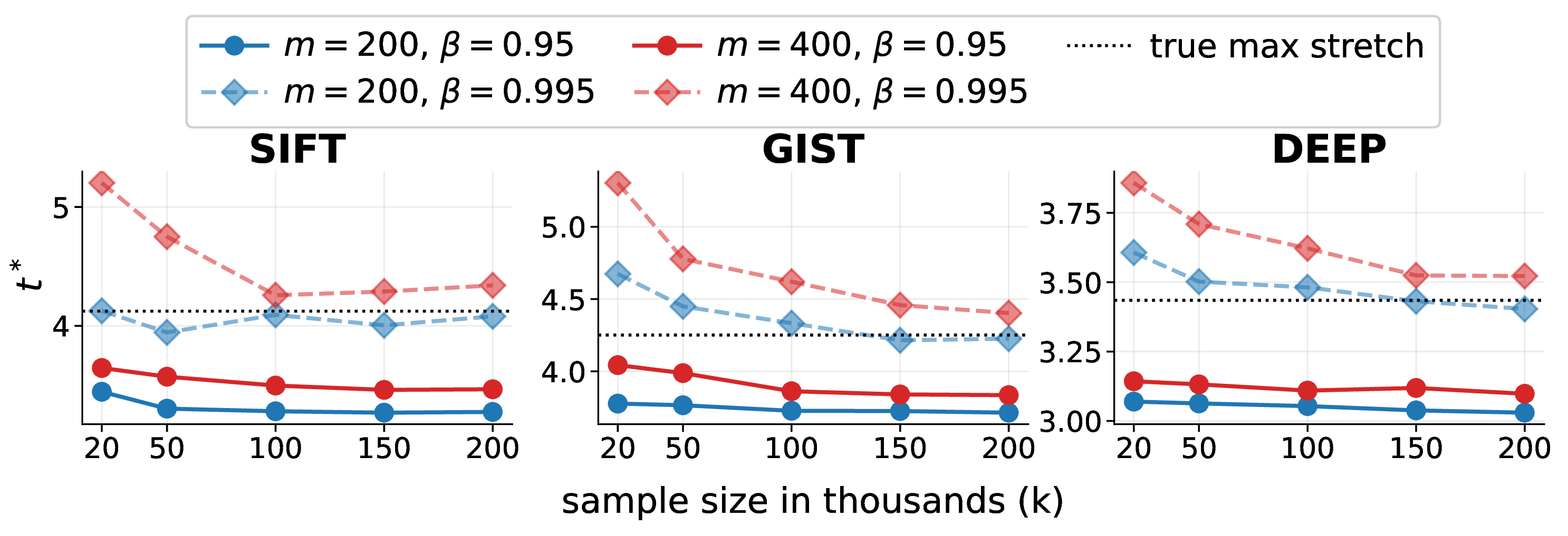
We validate our stochastic stretch estimation and characterize its sensitivity to key EVT hyperparameters using the level-2 HNSW subgraph, where the true maximum stretch \(t_{emp}\) is computable by brute force over a tractable number of nodes6. We ablate the two parameters that must be committed to before sampling—confidence level \(\beta\) and block count \(m\)—across \((\beta, m) \in \{0.95, 0.995\} \times \{200, 400\}\) and vary sample size to generate four stretch value curves, using the brute-force \(t_{emp}\) as ground truth. Test is conducted on SIFT, GIST, and DEEP with \(M{=}32, ef_c{=}100\).
In Figure 6, we show that higher \(\beta\) consistently raises \(t^*\) since it selects a higher quantile of the fitted GEV and is more conservative. A larger block count (\(m{=}400\)) yields higher, more conservative estimates than \(m{=}200\): more blocks supply more fitting points to the GEV, enabling better characterization of the upper tail of stretch values, whereas fewer blocks underfit the extremes. This comes at a convergence cost—\(m{=}400\) saturates more slowly because smaller per-block samples produce more variable block maxima, so the fitted return level continues drifting as sample size grows rather than leveling off. Despite these differences, all \((\beta, m)\) configurations yield a stable fitted \(t^*\)—one whose value no longer changes meaningfully with additional samples—by approximately 150k sampled pairs across all three datasets. High-confidence settings (\(\beta{=}0.995\)) with large \(m\) consistently yield estimates that bound the true empirical stretch with a safe margin, whereas lower-confidence configurations reduce estimation accuracy. Therefore, for base-layer operation in later sections we use the conservative \(m{=}400\), \(\beta{=}0.995\) setting to mitigate stretch underestimation probability.
7.3 Stretch and HNSW Construction Parameters↩︎
To further investigate how HNSW construction parameters influence the empirical maximum stretch of the resulting graph, we adopt the same Stochastic Stretch Estimation (SSE) procedure described in Section 7.2 and repeat it for graphs derived from various HNSW construction parameters. We report the estimated stretch across SIFT1M and DEEP1M, and use a parameter grid spanning \(M \in \{16,32,48,64\}\), \(ef_c \in \{100,200,300\}\), with \(\beta = 0.995\) fixed throughout. The results are presented in Figure 7.
The graph shows that for fixed \(ef_c\), increasing \(M\) consistently reduces the stretch, reflecting improved graph connectivity. Similarly, for fixed \(M\), larger \(ef_c\) yields lower stretch, indicating higher-quality nearest-neighbor connections during construction. These findings align with the role of HNSW construction in shaping the graph’s effective spanner properties and its associated stretch behavior.

| Dataset | Metric | \(M=16,\,ef_c=100\) | \(M=16,\,ef_c=200\) | \(M=32,\,ef_c=100\) | \(M=32,\,ef_c=200\) | ||||||||
| \(k\) | 10 | 50 | 100 | 10 | 50 | 100 | 10 | 50 | 100 | 10 | 50 | 100 | |
| SIFT1M | \(t\) | 4.059 | 4.059 | 4.059 | 3.853 | 3.853 | 3.853 | 3.657 | 3.657 | 3.657 | 3.601 | 3.601 | 3.601 |
| SBE-NN | 48.95 | 50.54 | 51.41 | 48.16 | 49.66 | 50.47 | 47.42 | 48.59 | 49.21 | 48.47 | 50.00 | 50.83 | |
| SBE-NN+LBP&EP | 40.07 | 42.31 | 43.20 | 39.95 | 43.14 | 44.61 | 39.30 | 42.24 | 43.54 | 40.67 | 43.84 | 45.32 | |
| SBE-Q | 5.60 | 14.07 | 18.66 | 4.04 | 11.38 | 15.82 | 3.40 | 10.13 | 14.22 | 3.62 | 10.37 | 14.67 | |
| SBE-Q+LBP | 4.01 | 11.19 | 15.54 | 2.88 | 8.95 | 12.99 | 2.45 | 7.85 | 11.60 | 2.57 | 8.23 | 12.11 | |
| MBV | 3.85 | 6.37 | 7.91 | 2.80 | 4.84 | 6.08 | 2.38 | 4.33 | 5.51 | 2.51 | 4.59 | 5.89 | |
| DEEP1M | \(t\) | 4.251 | 4.251 | 4.251 | 4.148 | 4.148 | 4.148 | 4.067 | 4.067 | 4.067 | 3.867 | 3.867 | 3.867 |
| SBE-NN | 81.03 | 84.75 | 86.52 | 71.36 | 76.12 | 78.40 | 83.43 | 86.86 | 88.51 | 83.08 | 86.53 | 88.19 | |
| SBE-NN+LBP&EP | 70.88 | 76.72 | 79.33 | 55.45 | 61.76 | 64.69 | 73.95 | 79.45 | 81.86 | 72.84 | 78.49 | 80.99 | |
| SBE-Q | 3.82 | 12.60 | 20.89 | 1.39 | 5.96 | 15.82 | 4.71 | 14.32 | 20.03 | 3.65 | 12.64 | 19.07 | |
| SBE-Q+LBP | 3.48 | 10.04 | 17.23 | 1.22 | 4.35 | 13.29 | 4.12 | 11.49 | 16.09 | 3.08 | 9.51 | 14.72 | |
| MBV | 3.29 | 6.46 | 10.11 | 1.20 | 2.73 | 9.48 | 4.07 | 7.77 | 8.52 | 3.05 | 6.70 | 8.40 | |
| GIST1M | \(t\) | 4.470 | 4.470 | 4.470 | 4.119 | 4.119 | 4.119 | 3.930 | 3.930 | 3.930 | 3.646 | 3.646 | 3.646 |
| SBE-NN | 84.91 | 86.08 | 86.63 | 83.83 | 85.15 | 85.77 | 85.10 | 86.40 | 87.01 | 83.95 | 85.26 | 85.87 | |
| SBE-NN+LBP&EP | 80.27 | 81.64 | 82.27 | 77.69 | 79.22 | 79.93 | 78.98 | 80.55 | 81.26 | 76.31 | 78.05 | 78.85 | |
| SBE-Q | 15.67 | 31.42 | 38.75 | 10.04 | 23.54 | 30.90 | 9.42 | 22.89 | 30.39 | 6.66 | 17.26 | 24.07 | |
| SBE-Q+LBP | 15.49 | 28.52 | 35.71 | 9.75 | 20.95 | 27.85 | 8.96 | 19.88 | 27.08 | 5.80 | 14.25 | 20.42 | |
| MBV | 15.01 | 23.62 | 26.04 | 9.70 | 16.55 | 18.58 | 8.94 | 15.58 | 17.52 | 5.64 | 11.47 | 13.15 | |
5pt
7.4 System Ablation↩︎
We compare the number of distance computations (NDC) required to return the true \(k\) nearest neighbors across system variants. For ease of display, NDC is reported as a percentage of the total number of base nodes in the 1M-size datasets we use (NDC % of 1M), eg. 1% means we did 10k distance computations. Experiments fix \(ef_s{=}100\) and vary \(k\in\{10,50,100\}\). We evaluate four index configurations \((M,\,ef_c)\in\{16,32\}\times\{100,200\}\) on three datasets (SIFT1M, DEEP1M, GIST1M). This experiment is independent of the final certification stage and no target recall is enforced.
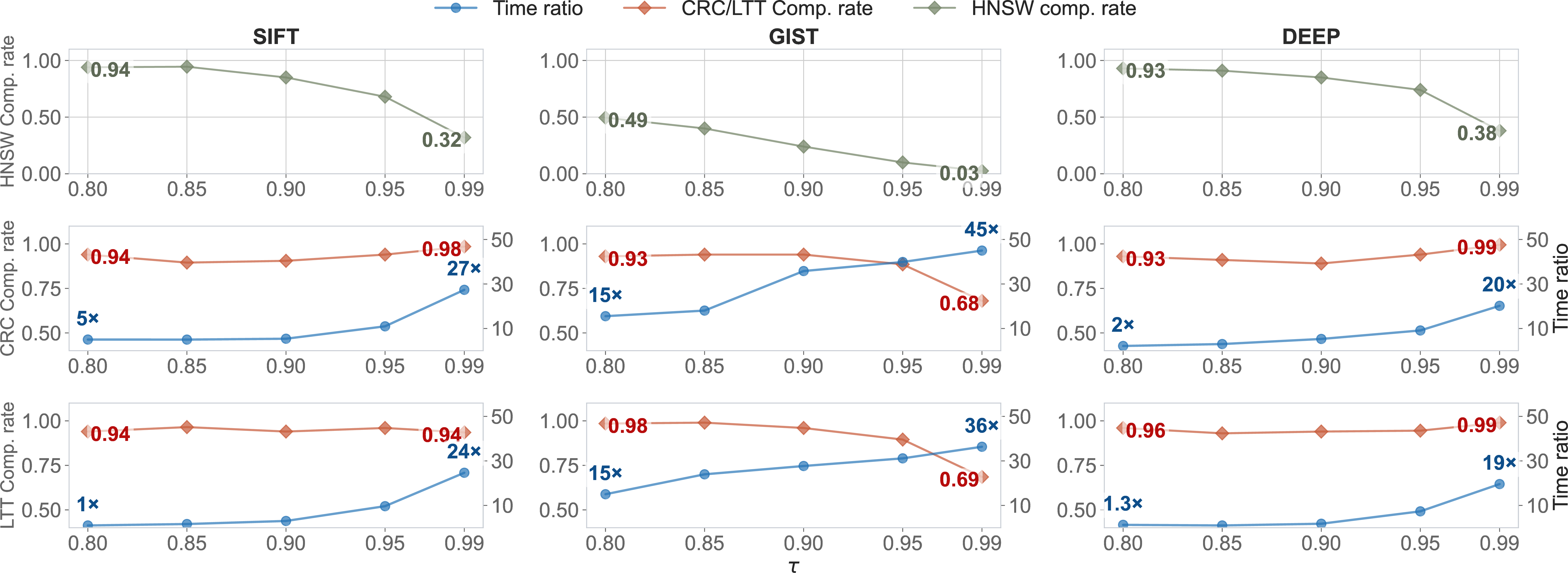
Experimental setup. In these experiments, we fix the underlying HNSW parameters to \(M{=}32\), \(ef_c{=}200\), and \(ef_s{=}100\). Results are averaged over 100 random queries. In Figure 8, panels (a)–(c) show CRC and panels (d)–(f) show LTT on the three datasets. We fix the target recall threshold to \(\tau{=}0.90\), and for LTT we set \(\epsilon{=}0.5\). Each blue point is an operating point obtained by varying \(\alpha\), and the numeric annotation next to the point is the corresponding \(\alpha\) value; runtime is reported on the x-axis as a multiple of plain HNSW under the same configuration. In Figure 9, we keep the same HNSW configuration and vary \(\tau\), with \(\alpha{=}0.05\) and \(\epsilon{=}0.5\) specifically for LTT; panels (a)–(c) show plain HNSW, panels (d)–(f) show CRC, and panels (g)–(i) show LTT.
Compared variants. We organise the variants into two families and compare five of them. The baselines,SBE-NN and SBE-Q, are expansion strategies that identify candidate nodes within the stretch-bounded radius without any pruning of final distance computations.Applying the methods lower-bound pruning (LBP) and elliptical pruning (EP) on top of SBE-NN yields SBE-NN+LBP&EP,and on SBE-Q gives the proposed MBV. To isolate the individual contribution of LBP and EP,we additionally include SBE-Q+LBP, which applies only the LBP component to SBE-Q;the gap between SBE-Q+LBP and MBV in Table 2 quantifies the saving attributable to EP.
Results. Table 2 reveals two consistent trends. First, SBE-Q is a substantially stronger baseline than SBE-NN across all configurations, owing to its smaller expansion radius: eliminating the additive \(\hat{d}_1\) term present in SBE-NN dramatically shrinks the graph region explored during rectification. Building on SBE-Q, applying LBP (SBE-Q+LBP) further reduces NDC by \(14.3\)–\(26.4\%\) across configurations relative to SBE-Q alone. Adding EP on top (MBV) achieves an additional \(25.8\)–\(58.3\%\) reduction across configurations by adaptively tightening the truncation radius as the running maximum of discovered \(k\)-NN distances decreases during Dijkstra traversal. Overall, the effect of augmenting SBE-Q with MBV is more pronounced in \(k=50\) or \(k=100\), as the larger \(d_k\) leads to a larger expansion radius, resulting in more nodes to explore and more pruning opportunities. MBV is consequently our best-performing method: on SIFT1M it reduces NDC to as low as \(2.51\%\) of base nodes at the finest index configuration for small \(k\), and to around \(5.6\%\) on the higher-dimensionality and harder GIST1M dataset. Second, a cross-configuration trend mirrors the stretch estimation results: finer graphs (larger \(M\) or \(ef_c\)) yield smaller \(t^{*}\), which in turn shrinks the expansion radius \(t^{*}\times\hat{d}_k\) and lowers NDC for all five variants. Both trends above are consistent across different \(k\).
7.5 Recall Target Compliance of Conformal Parameters↩︎
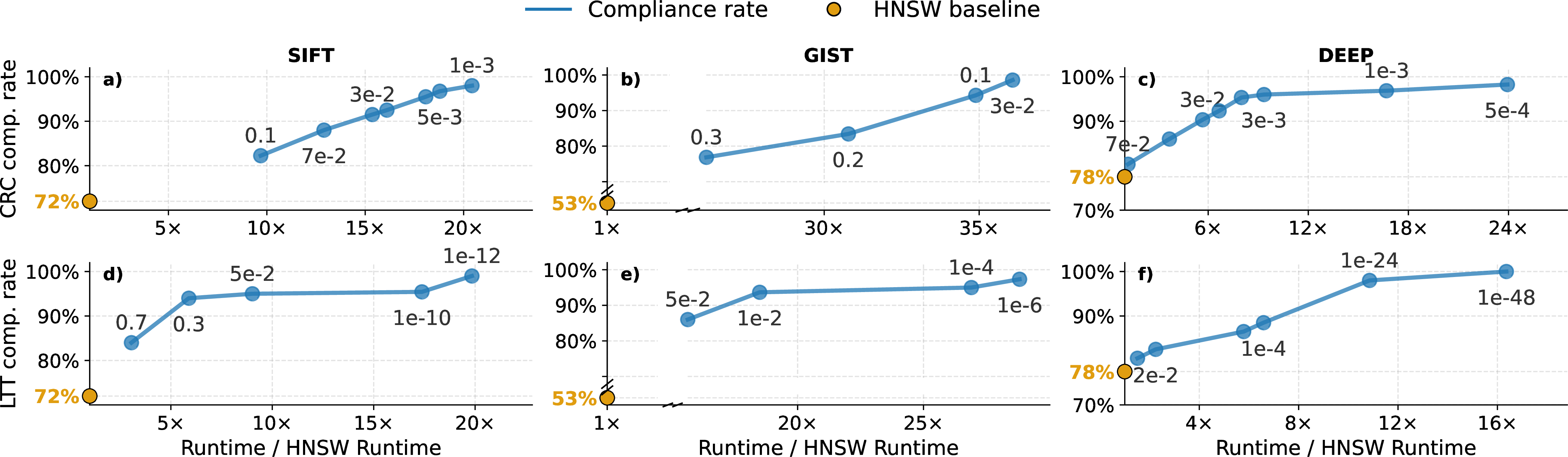

We next evaluate how the conformal parameters affect the final recall–runtime trade-off of CTR via the CRC/LTT. Rather than reporting average recall, we utilize per-query result-set compliance from Section 6.1 and report the compliance rate over a set of queries, which is the fraction of queries for which \(Recall(q){\ge} \tau\). Compliance rate is based on the result set after the rectification step, if certification fails.
In these experiments, we fix the underlying HNSW parameters to \(M{=}32\), \(ef_c{=}200\), and \(ef_s{=}100\). In Figure 8, panels (a)–(c) show CRC and panels (d)–(f) show LTT on the three datasets. We fix the target recall threshold to \(\tau{=}0.90\), and for LTT we set \(\epsilon{=}0.5\). Each blue point is an operating point obtained by varying \(\alpha\), and the numeric annotation next to the point is the corresponding \(\alpha\) value; runtime is reported on the x-axis as a multiple of plain HNSW under the same configuration. In Figure 9, we keep the same HNSW configuration and vary \(\tau\), with \(\alpha{=}0.05\) and \(\epsilon{=}0.5\); panels (a)–(c) show plain HNSW, panels (d)–(f) show CRC, and panels (g)–(i) show LTT.
Results. In Figure 8, for both CRC and LTT, decreasing \(\alpha\) makes certification stricter, so fewer HNSW outputs are certified directly and more queries are rectified. This raises the compliance rate but also increases runtime; larger \(\alpha\) has the opposite effect. Across the \(\tau\)-sweeps in Figure 9, the compliance rate of plain HNSW (\(ef_s{=}100\)) drops quickly as \(\tau\) increases, whereas both CTR variants remain much flatter because rectification preserves compliance on hard queries at the cost of higher runtime ratio. Specifically, at high \(\tau\) values (eg. \(\tau=0.9, 0.99\)), HNSW fails the target recall more often, and the expensive MBV is invoked by the certifier more frequently, resulting in increased CTR runtime7.
Comparing the two certifiers, LTT achieves higher compliance at comparable runtime ratios. This improvement comes from LTT’s stricter per-query guarantee, which enables a more selective allocation of the heavier MBV computation to queries that are more likely to have low recall and therefore contribute the most to compliance gains. Take the \(\alpha\)-sweep for GIST in Figure 8 for example, under the \(\alpha=5 \times 10^{-2}\) setting, LTT has four fewer false negatives and one fewer false positive than CRC in the runtime-comparable \(\alpha=0.3\) setting. We further verified that the recall shortfall of both CRC and LTT is below the respective expected and probabilistic bounds stated in Theorem 5, across all values of \(\tau\), \(\alpha\), \(\epsilon\), and \(\beta\) (for stretch estimation as experiment setup) used in these experiments, validating our theorem empirically.
Notably, the small \(\alpha\) values that appear in LTT are largely an inherent consequence of the test itself: the null benchmark is the boundary case with \(x_\theta\) failures among \(m_\theta\) certified queries under a Binomial\((m_\theta,\epsilon)\) model, and the corresponding one-sided tail probability can become extremely small as soon as the observed failure count falls below the nominal level \(\epsilon m_\theta\). Thus, the practically useful range of \(\alpha\) in LTT is naturally shifted toward smaller values; this is a property of the testing mechanism rather than an unusually aggressive confidence requirement.
Figure 10 further illustrates how the LTT threshold \(\theta\) varies jointly with \(\alpha\) and \(\epsilon\). The qualitative trend of \(\theta\) varying with \(\alpha\) and \(\epsilon\) is consistent. In particular, along a fixed-\(\epsilon\) slice of the surface, decreasing \(\alpha\) increases the selected threshold \(\theta\). Since LTT certifies a query only when its score exceeds \(\theta\), a larger threshold makes certification more selective: fewer queries are accepted directly, more queries are sent to rectification, and the final compliance rate increases at the cost of higher latency. Conversely, for the same fixed \(\epsilon\), increasing \(\alpha\) lowers \(\theta\), which certifies more queries directly and therefore reduces runtime, but also lowers compliance. To visually illustrate this trade-off, the black contour lines in Figure 10 depict constant-\(\epsilon\) cross-sections of the threshold surface: \(\epsilon{=}0.4\) for SIFT1M and DEEP1M, and \(\epsilon{=}0.7\) for GIST1M. Each such cross-section isolates the one-dimensional family of operating points obtained by varying \(\alpha\) while holding \(\epsilon\) fixed, thereby making clear how the resulting change in \(\theta\) governs the latency–compliance trade-off described above. The figure also suggests a practical tuning strategy: first select \(\epsilon\) so as to avoid the broad plateau region of \(\theta\) (the yellow region, where variation in \(\epsilon\) has relatively little effect on the threshold), and then vary \(\alpha\) to choose the desired operating point along the corresponding constant-\(\epsilon\) trade-off curve.
We next study how the HNSW operating point affects the latency–compliance trade-off. In Figure 11, blue/green use \(M{=}16\) and red/brown use \(M{=}32\); blue/red use \(ef_s{=}200\), while green/brown use \(ef_s{=}300\). Panels (a)–(c) show CRC and panels (d)–(f) show LTT for SIFT, GIST, and DEEP. Across the rerun, increasing \(ef_s\) generally shifts curves upward and left, and increasing \(M\) produces a similar improvement in these operating ranges. The reason is that both changes improve the quality of the initial HNSW search: larger \(ef_s\) explores more candidates at query time, while larger \(M\) gives the graph more connectivity. As a result, more queries already meet the compliance target before rectification, so the expensive recovery step is triggered less often. This lowers the runtime ratio needed to reach a given compliance rate. Overall, Figure 11 suggests that \(ef_s\) is the cleaner query-time knob, while \(M\) provides a stronger index-level operating point when its memory and build-time cost is acceptable.
The CTR framework naturally extends to filtered search on top of algorithms such as ACORN [2]. We present our results in Section 8.2.
7.6 Repeated Certification↩︎
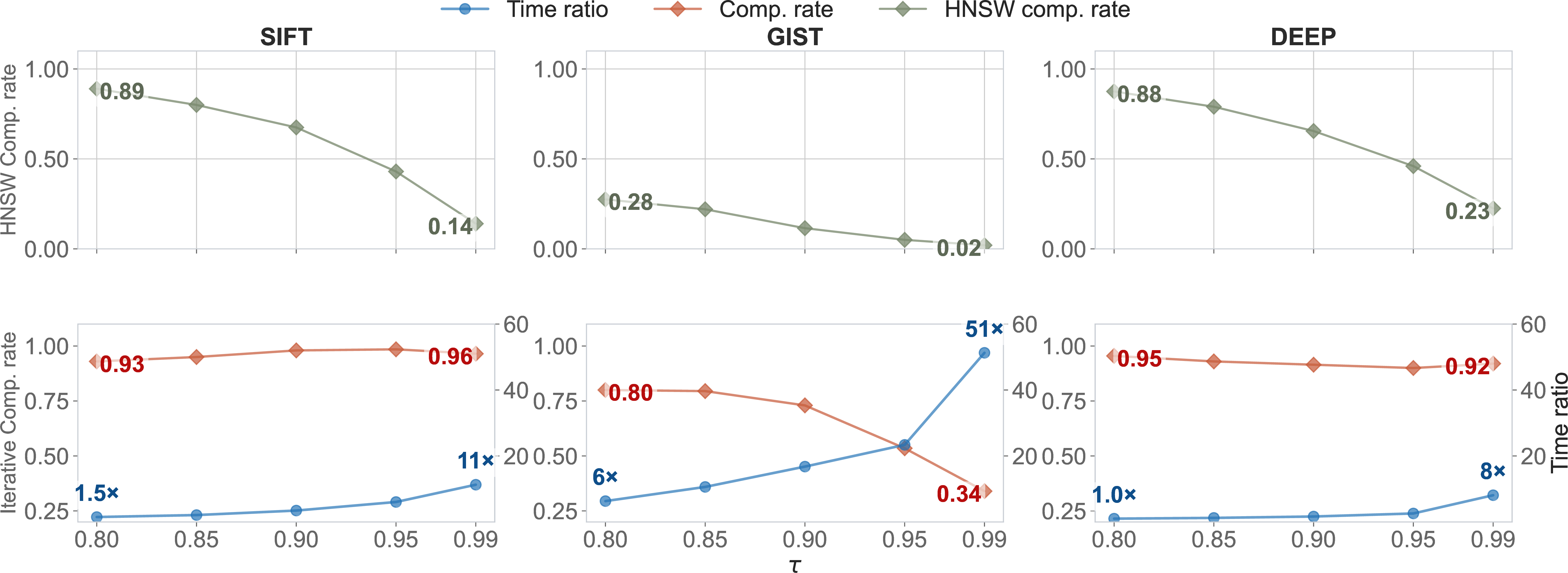
Motivation. Section 7.5 shows that at high \(\tau\), HNSW fails the target recall on a growing share of queries, so the certifier escalates to the expensive exact MBV rectification more often and CTR’s runtime ratio increases accordingly. As an alternative to invoking MBV, we explore repeating the certification attempt with an expanded search radius: instead of exactly rectifying a query that fails certification, we simply re-run HNSW at a larger \(ef_s\) and re-certify, hoping that the extra candidates already push the result into compliance without ever paying for exact recovery. This policy trades the correctness guarantee of exact rectification for the hope of a cheaper, purely HNSW-side fix, and we study whether this mitigates the runtime increase from Section 7.5 while keeping recall competitive.
Experimental setup. The repeated-certification policy proceeds as follows. Starting from \(ef_s{=}100\), we run HNSW and score the result with a CRC certifier calibrated at that \(ef_s\) and the target \(\tau\); if the certifier accepts, we stop and return the current result. Otherwise we increase \(ef_s\) by \(100\), re-run HNSW at the new, larger radius, and re-certify with a separately calibrated certifier for that \(ef_s\); this repeats until certification succeeds or \(ef_s\) reaches \(ef_{max}{=}1000\), at which point the last HNSW result is returned regardless of certifier outcome. No MBV or other exact-recovery step is ever invoked. Crucially, this requires calibrating one CRC certifier per \(ef_s\) value—ten certifiers, one each for \(ef_s \in \{100, 200, \dots, 1000\}\), for every (dataset, \(\tau\)) pair—rather than a single certifier as in Section 7.5. All certifiers are calibrated offline, on the held-out calibration split (with size being 80% of the #queries column in Table 1) before any online evaluation begins; at query time the appropriate pre-fit certifier is simply looked up for the current \(ef_s\) and applied, so this calibration cost is a one-time offline expense and is not counted in the online per-query runtime ratios reported below. We fix \(k{=}100\) and \(\alpha{=}0.01\), sweep \(\tau \in \{0.80, 0.85, 0.90, 0.95, 0.99\}\), and evaluate on \(200\) held-out queries per dataset on SIFT1M, GIST1M, and DEEP1M.
Results. Figure 12 shows that, on SIFT1M and DEEP1M, repeated certification substantially mitigates the runtime increase seen with the rectifier in Section 7.5 while keeping recall on a similar level: on SIFT1M the runtime ratio only grows from \(1.5\times\) to \(11\times\) across the \(\tau\)-sweep (versus \(1\times\)–\(24\times\) for the LTT rectifier) while compliance stays at \(0.93\)–\(0.96\) (versus \(0.94\)–\(0.97\) for the rectifier); on DEEP1M the runtime ratio grows from \(1.0\times\) to \(8\times\) (versus \(1.3\times\)–\(19\times\) for the rectifier) while compliance stays at \(0.92\)–\(0.95\) (versus \(0.96\)–\(0.99\) for the rectifier).
On GIST1M, however, the policy performs markedly worse, especially at high \(\tau\): compliance falls from \(0.80\) at \(\tau{=}0.80\) to just \(0.34\) at \(\tau{=}0.99\), even as the runtime ratio still climbs to \(51\times\). The reason is that GIST1M’s hard queries are hard precisely because plain HNSW cannot reach them: the top row of Figure 12 shows the HNSW baseline compliance rate on GIST1M collapsing to \(0.02\) at \(\tau{=}0.99\), meaning almost no query is compliant at \(ef_s{=}100\). Repeated certification responds to this by escalating \(ef_s\) into the thousands on these queries, but pushing \(ef_s\) arbitrarily high does not guarantee that HNSW’s beam search actually surfaces the true nearest neighbors it is missing; many attempts are spent re-searching without ever satisfying the certifier, so both runtime and the miss rate grow together. The rectifier, by contrast, still reaches 70% compliance on GIST1M at \(\tau{=}0.99\) (versus \(0.34\) for repeated certification) because MBV guarantees exact recovery of the true \(k\)-nearest neighbors whenever it is invoked (Lemma 1), rather than merely hoping a larger beam finds them. Overall, these results indicate that repeated certification is an attractive lower-cost alternative when the underlying HNSW index has enough residual capacity to reach the target recall through search-radius expansion alone (SIFT1M, DEEP1M), but exact rectification remains preferable whenever queries are difficult and the compliance target is stringent, since only rectification offers a correctness guarantee independent of how well HNSW itself performs.
7.7 Scalability Experiments↩︎
A natural concern is whether dataset size adversely affects the runtime overhead of CTR: larger datasets contain more candidate nodes within any search radius, which could inflate the cost of SBE-Q. We test this using the Yandex Text-to-Image dataset8 at two scales—T2I-10M and T2I-100M—with index configuration \(M{=}32\), \(ef_c{=}200\) on normalized vectors, with an Intel Xeon Ice Lake 3.5 GHz processor with 64GB memory. For each scale, stretch estimation is carried out following the same procedure as Section 7.2 (\(\beta{=}0.995\), \(m{=}400\)). As we use a subset of T2I-1B, query ground truths were re-computed by brute-force.
| T2I-10M (t=4.133) | T2I-100M (t=4.124) | |||||
|---|---|---|---|---|---|---|
| \(k\) | 10 | 50 | 100 | 10 | 50 | 100 |
| million NDC | 0.55 | 1.16 | 1.55 | 2.33 | 4.63 | 6.11 |
| % of \(N\) | 5.55 | 11.64 | 15.51 | 2.33 | 4.63 | 6.11 |
5pt
We first run MBV without the certifier on 200 text queries sampled from T2I. Table 3 reports average NDC in absolute value and as a fraction of dataset size. Stretch estimation on 10M and 100M scales yields \(t\)=4.133 and \(t\)=4.124 respectively, confirming that the graph stretch does not grow appreciably with dataset size. At the same time, a \(10\times\) larger corpus means base vectors are distributed more densely in the ambient space: the \(k\)-th true neighbor of a typical query lies closer, so \(d_k\) decreases. Since the SBE-Q search radius equals \(t \cdot d_k\), a smaller \(d_k\) directly shrinks the expansion ball, and that ball covers a smaller fraction of the \(N\) base nodes. Table 3 reflects this exactly: the expansion fraction drops by roughly \(2.5\times\) across all \(k\) values when moving from 10M to 100M (eg. \(k{=}10\): \(5.55\%\to2.33\%\)). Recall is consistently 1 in all settings.
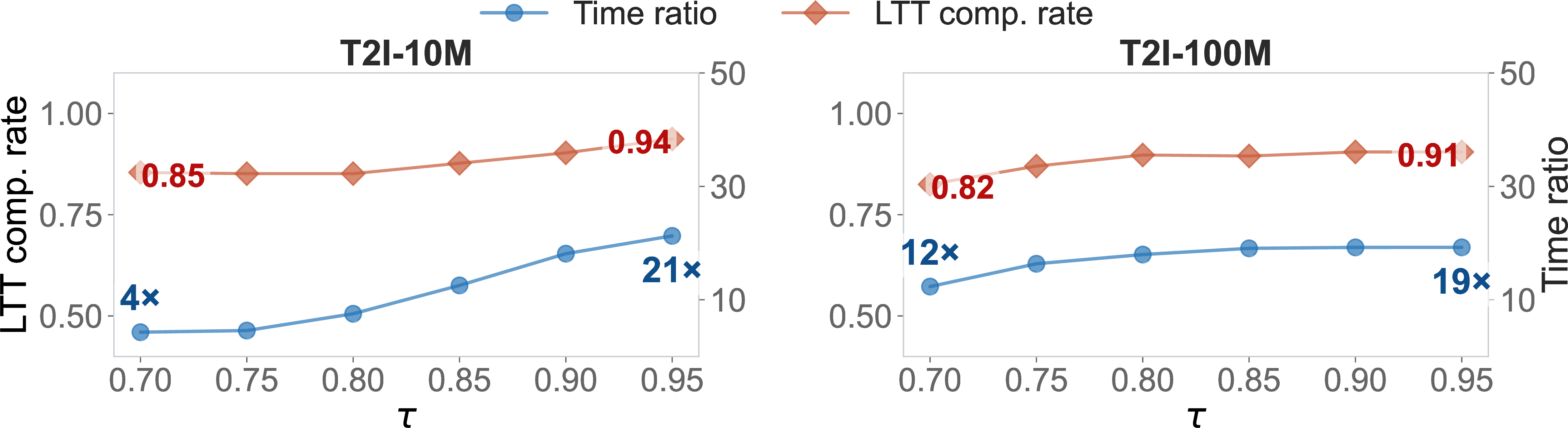
We next conduct a full \(\tau\)-sweep (\(ef_s{=}100\), \(k{=}100\)) to evaluate end-to-end overhead. Absolute latency increases with dataset size, as expected: HNSW grows by \(8\)–\(9.4\times\) and CTR by \(7.5\)–\(8.4\times\). The key question is whether CTR adds disproportionate overhead beyond this baseline HNSW growth. Figure 13 shows that the normalized runtime ratio remains comparable across scales: the peak ratio even decreases from \(21.3\times\) at 10M to \(19.2\times\) at 100M. Thus, because the expansion radius remains bounded, CTR preserves the compliance–runtime trade-off across scales and introduces no additional scaling bottleneck beyond HNSW itself.
7.8 ConANN vs.CTR↩︎
We now perform an end-to-end system comparison against ConANN [20], a recent ANN system that calibrates a conformal early-termination rule on an IVF index to also control approximation error and meet recall target. Both systems are evaluated on three datasets (SIFT1M, DEEP1M,and T2I-10M with normalized vectors), sweeping the recall target \(\tau\in\{0.80,0.85,0.90,0.95,0.99\}\) (points connected in order of increasing \(\tau\) values on graph) with \(k{=}100\); we report the per-query compliance rate \(\Pr[\mathrm{Recall}(q)\ge\tau]\) against end-to-end throughput.
Index configurations. ConANN indexes each dataset with IVF-Flat using \(1024\) Voronoi cells and exact \(L_2\) scoring within probed cells, \(\alpha\) calculated as \(1-\tau\). CTR runs on HNSW with \(M{=}32\), \(ef_c{=}200\), and query-time \(ef_s{=}100\); we certify each result with LTT (Section 6) and rectify queries that fail certification with MBV.
Results. Figure 14 reports the compliance–throughput trade-off. Across all three datasets CTR attains higher compliance than ConANN at every comparable target; the systems differ chiefly in where they sit on the throughput axis. On SIFT1M, CTR is throughput-competitive: at modest targets (\(\tau\!\le\!0.90\)) it is as fast or faster than ConANN—at \(\tau{=}0.85\) LTT sustains \(1.7\)k QPS at \(91\%\) compliance versus ConANN’s \(1.5\)k QPS at \(67\%\)—and only at stringent targets does ConANN regain a throughput edge (e.g.\(789\) versus \(97\) QPS at \(\tau{=}0.95\)), where its compliance nonetheless plateaus at \(0.72\)–\(0.82\) against CTR’s \(0.94\)–\(0.99\). The gap in compliance rate is a direct consequence of the certify-then-rectify mechanism: LTT supplies a per-query confidence guarantee, and this guarantee, combined with CTR’s ability to recover the exact nearest neighbors for queries flagged as low-quality, is what gives CTR its edge, lifting the recall of such queries toward 1 and raising the overall compliance rate. ConANN, by contrast, can only reorder and truncate its IVF probe and cannot exactly recover the neighbors it misses, so a fixed fraction of queries necessarily remains below \(\tau\) at every point.

7.9 DARTH vs. CRC/LTT↩︎
Recently, DARTH [3] was proposed solely as a predictor of recall. We therefore compare it directly against CRC and LTT in a certifier-only setting, i.e., without true neighbor rectification (as DARTH does not have this capability). Table 4 reports the F1 scores with respect to the binary event \(Recall(q)\ge\tau\). For fairness, we use DARTH only as a recall predictor and let HNSW run to the same stopping point in all methods, rather than using DARTH’s early-termination mechanism. The experiment is conducted on SIFT1M with \(M{=}32\), \(ef_c{=}200\), \(ef_s{=}100\), \(k{=}100\) and 1000 random queries, utilizing the implementation from the DARTH authors. Across all three target levels, CRC/LTT attain higher F1, with the gap becoming larger at stricter targets. Similar results were obtained across all data sets and are omitted for brevity. DARTH is a best-effort predictor and does not formally control the fraction of queries whose recall falls below the target. In contrast, CRC and LTT are calibrated for fixed deployment settings (dataset, index configuration, workload, and target recall \(\tau\)) and explicitly control compliance-related errors under that setting. Consequently, for deciding whether an HNSW result should be accepted as meeting a prescribed recall target, CRC/LTT yield a more reliable acceptance rule.
| \(\tau\) | DARTH | CTR | ||
| Default | Tuned | CRC | LTT | |
| 0.85 | 0.968 | 0.971 | 0.983 | 0.983 |
| 0.90 | 0.913 | 0.913 | 0.965 | 0.966 |
| 0.95 | 0.709 | 0.709 | 0.865 | 0.874 |
5pt
7.10 Extension to Disk-based Search↩︎
In real production settings, loading the full vector index into memory is often infeasible at billion-scale. Vector search methods that account for disk I/O are therefore necessary. In this section we show that CTR extends to such settings using DiskANN [13], which achieves state-of-the-art disk-based ANN performance by storing a Vamana graph index on disk and exploiting beam-search with asynchronous I/O to amortise latency across concurrent node fetches.
Experimental Setup. We consider three settings. (1) In-memory: the Vamana graph variant of DiskANN, where the full graph with full-precision vectors is loaded into memory prior to ANN search. We use an Intel Ice Lake node with 64GB DDR4 unified memory. (2) Limited memory: memory is insufficient to hold the entire database. (3) Heavier disk-IO We additionally increase result size \(k\) based on the limited memory setting to assess the impact on disk-IO brought by an increased MBV expansion radius, which scales with \(t\cdot d_k\).
DiskANN search retains only quantized vectors and graph edges in memory while exact vectors reside on disk. To preserve the exactness guarantees of our algorithm, we forgo the quantized vectors and instead keep precomputed graph edge weights in memory, which costs \(\sim\)2.6GB on the T2I-10M graph (\(R{=}64\)). The MBV algorithm is otherwise unchanged: it performs Dijkstra expansion using solely these in-memory graph edges; the only difference is that exact distance computations (Algorithm 5, line 25) issue disk reads on cache misses. In this setting, we use an Intel Ice Lake node with 8GB DDR4 memory attached to a 75GB local NVMe drive. Experiments use the T2I-10M dataset; when fully loaded, it requires \(\sim\)8GB for base vectors and \(\sim\)2.6GB for the graph (\(R{=}64\)), totalling \(\sim\)10.6GB—exceeding the 8GB constraint but well within the 64GB limit of Setting 1. For all settings we run a \(\tau\)-sweep following Section 7.5, using LTT for all conformal predictors. Settings (1) and (2) results in the left and right panels of Figure 15 respectively; setting (3) results in Figure 16.
Parameters. We evaluate setting 1, 2 with \(k =10\) and setting 3 with \(k=20\). We use \(\alpha=0.1\), \(\varepsilon=0.5\), and \(\tau\in\{0.75,0.80,0.85,0.90,0.95\}\). The DiskANN index is built with maximum degree \(R=64\) and construction list size \(L_{\text{build}}=100\); search uses list size \(L=100\) and disk beam width \(B=2\). MBV is initialised from a single seed with 10,000 hot-cached nodes in Vamana
mode. Disk reads are issued via io_uring in basic single-issuer mode with direct I/O and a submit-batch size of 8, using a single thread. The MBV graph stretch parameter \(t=3.71\) is estimated following
Section 7.2.
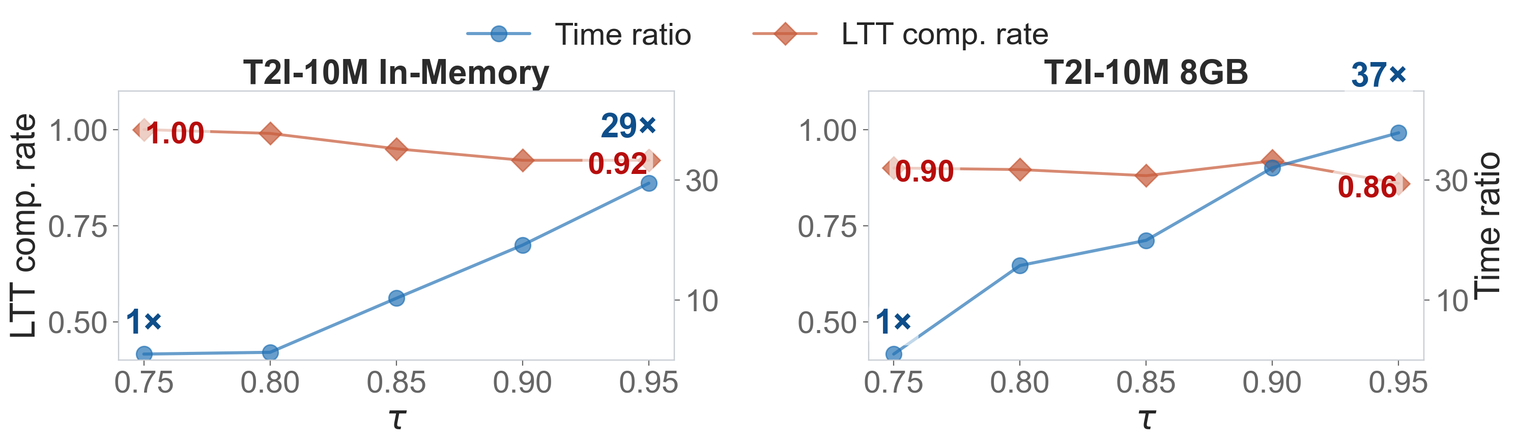
Results. As shown in Figure 15, the in-memory Vamana setting (left panel) confirms that CTR generalises beyond HNSW: it extends directly to the Vamana graph and achieves compliance–runtime trade-offs comparable to those observed on HNSW in Figure 9 of Section 7.5. In the limited-memory setting with \(k{=}10\) (right panel of Figure 15), the additional disk I/O incurred by MBV expansion remains controlled, adding 8–10\(\times\) DiskANN time to the runtime ratio at each \(\tau\) level. Notably, compliance rates in the limited-memory setting are consistently lower than in the in-memory setting. This gap arises because native DiskANN beam search relies on quantized vectors as distance proxies, yielding a weaker ANN baseline than exact Vamana search; as a result, the conformal certifier operates on lower-quality candidates, reducing the fraction of queries that pass certification.
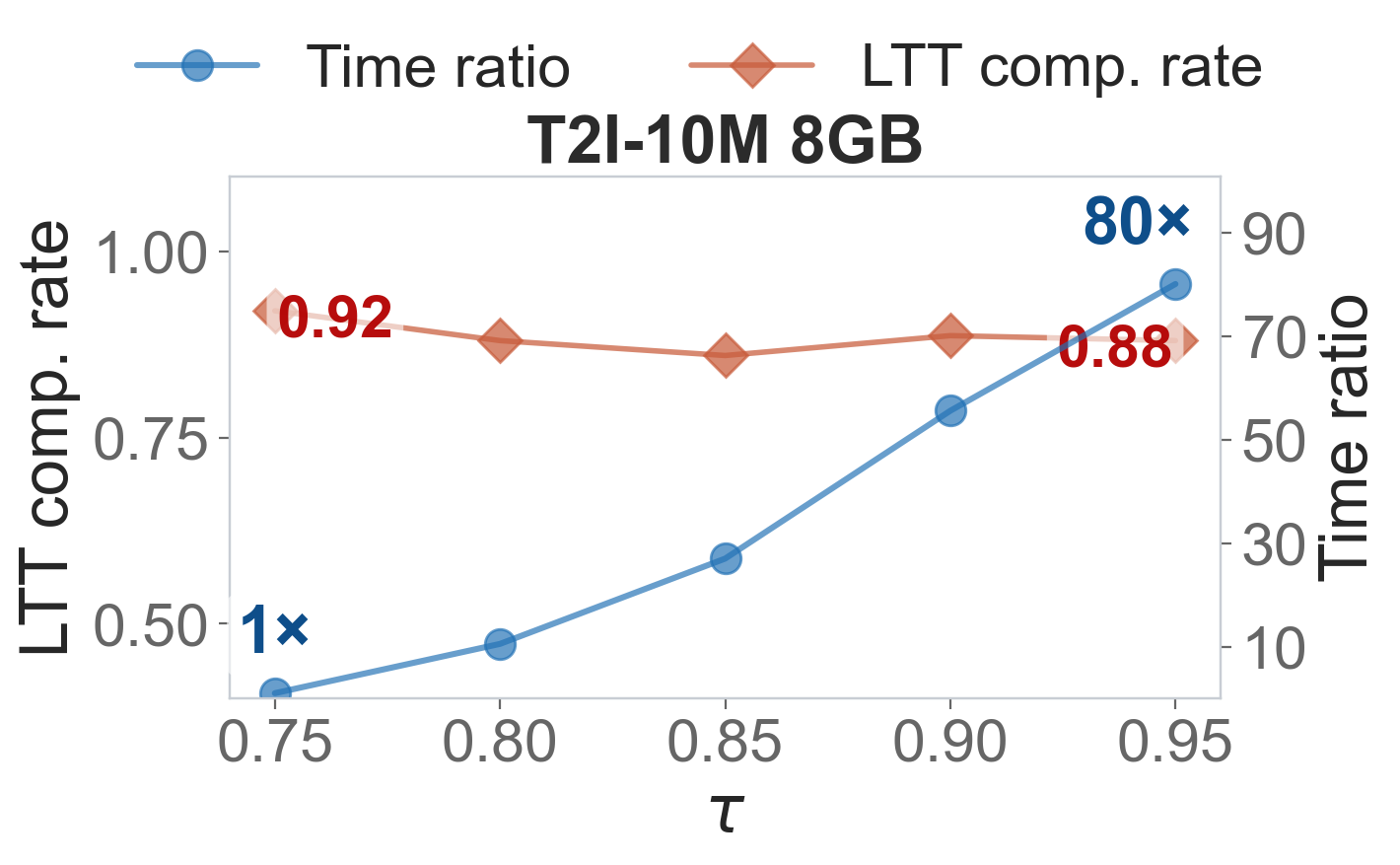
For setting (3), Figure 16 shows the effect of increasing \(k\) from 10 to 20. This enlarges the MBV search radius (\(t\cdot d_k\) grows as \(d_k\) increases with \(k\)), expanding the explored graph fraction by approximately 70% for queries that fail certification and thereby increasing disk I/O. This is directly reflected in the runtime ratio: at \(\tau{=}0.9\), the ratio rises from approximately \(30\times\) to \(50\times\) the DiskANN baseline. Overall, MBV transfers the recall–runtime trade-off observed from HNSW to disk-based vector search without any algorithmic modification.
8 Filtered Stretch-Bounded Expansion from Query (F-SBE-Q)↩︎
In this Section, we show the CTR methodology can be directly extended to handle filtered ANN search (FANNS), and provide experimental results of our implementation. In FANNS, the goal is to retrieve the approximate \(k\)-nearest neighbors that satisfy a specific predicate condition \(P\). Standard heuristic traversals often fail in these scenarios when filters disconnect the “small world” topology. However, by leveraging the global connectivity of the underlying graph structure—regardless of the predicate status of intermediate nodes—we can guarantee exact recovery of true nearest neighbors using the bounds derived from the approximate search results.
Remark (CTR Modifications for FANNS). The CTR pipeline requires only minimal modification to support FANNS. Deriving F-SBE-Q from SBE-Q entails a single algorithmic change: lines 25–30 of Algorithm 17 are augmented to check the predicate prior to computing the distance. The lower-bound and elliptical pruning techniques carry over unchanged, since the distance metric is independent of predicate membership—any candidate node that cannot be closer to \(q\) than the \(k\)-th approximate neighbor, by the triangle inequality, may be pruned regardless of whether it satisfies \(P\). The conformal predictor features defined in Section 6 are likewise applied to FANNS without modification.
8.0.1 Problem Formulation↩︎
Let \(P: \mathcal{X} \rightarrow \{0,1\}\) be a boolean predicate function. We seek the set of \(k\) nearest neighbors \(\mathcal{N}_{k,P}^*(q)\) such that for all \(x \in \mathcal{N}_{k,P}^*(q)\), \(P(x)=1\). Let \(d_{k,P}^*\) denote the distance to the true \(k\)-th nearest neighbor in the satisfying set: \[d_{k,P}^* = \max_{x \in \mathcal{N}_{k,P}^*(q)} \mathit{dist}(q, x)\] Let \(\mathcal{H}_{found}\) be the set of candidates returned by the initial HNSW search (or any heuristic phase). We identify the subset of these candidates that satisfy the predicate \(P\). If at least \(k\) such candidates exist, let \(\hat{d}_{k,P}\) denote the distance to the \(k\)-th closest satisfying candidate found so far.
Similar to the unfiltered case, the distance to the \(k\)-th candidate found by any approximate method is an upper bound on the true \(k\)-th distance: \[d_{k,P}^* \le \hat{d}_{k,P}\]
8.0.2 Theoretical Guarantees↩︎
We extend Theorem 3 to the filtered case using the observable bound \(\hat{d}_{k,P}\). The critical insight is that while the targets must satisfy \(P\), the path taken in the graph \(G'\) to reach them need not. Thus, we rely on the spanner property of the full augmented graph \(G'\).
Theorem 6 (Filtered SBE-Q). Let \(q\) be a query point virtually inserted into the graph \(G\) such that the augmented graph \(G'\) is a \(t'\)-spanner. Let \(\hat{d}_{k,P}\) be the distance to the \(k\)-th approximate neighbor satisfying predicate \(P\) (as returned by HNSW or updated dynamically). Then, every true filtered top-\(k\) point lies inside the graph ball of radius \(t' \cdot \hat{d}_{k,P}\) centered at \(q\).
Formally, for every \(x^* \in \mathcal{N}_{k,P}^*(q)\): \[d_{G'}(q, x^*) \le t' \cdot \hat{d}_{k,P}\]
Proof. Let \(x^*\) be any arbitrary point in the true filtered set \(\mathcal{N}_{k,P}^*(q)\). By definition of the true set and the upper bound property of the approximate results: \[\mathit{dist}(q,x^*) \le d_{k,P}^* \le \hat{d}_{k,P}\] Since the augmented graph \(G'\) is a \(t'\)-spanner over the full set of vertices \(V \cup \{q\}\), there exists a path between \(q\) and \(x^*\) in \(G'\) such that: \[d_{G'}(q,x^*) \le t' \cdot \mathit{dist}(q, x^*)\] Substituting the metric bound: \[d_{G'}(q,x^*) \le t' \cdot \hat{d}_{k,P}\] Thus, the search radius defined by the approximate results is sufficient to encompass all true answers. ◻
8.0.3 Algorithm↩︎
The expansion algorithm (Algorithm 17) proceeds by traversing the graph \(G'\) starting from \(q\). Crucially, to preserve the spanner property \(t'\), the traversal visits nodes regardless of whether they satisfy \(P\). The predicate \(P(v)\) is checked only during the candidate collection phase to update the dynamic bound \(\hat{d}_{k,P}\). While Algorithm 17 presents the logic for predicate handling, in practice, this traversal is further optimized using the Metric Bound Verification techniques we introduce in Section 5.
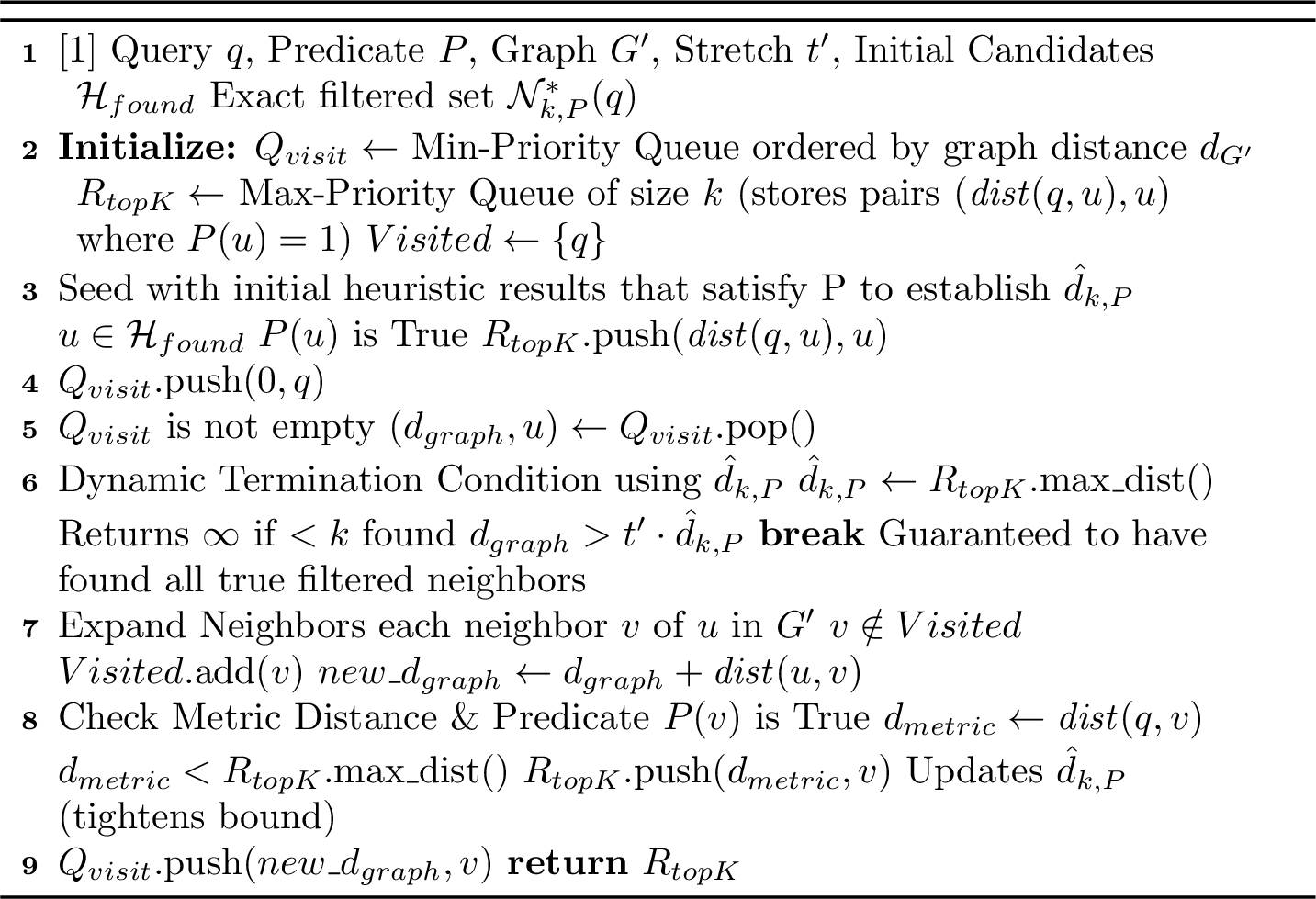
| Dataset | Metric | \(M{=}16,M_\beta{=}32,ef_c{=}200,k{=}10\) | \(M{=}16,M_\beta{=}32,ef_c{=}200,k{=}100\) | \(M{=}32,M_\beta{=}64,ef_c{=}200,k{=}10\) | \(M{=}32,M_\beta{=}64,ef_c{=}200,k{=}100\) | ||||||||||||
| \(\sigma\) | 1 | 5 | 10 | 25 | 1 | 5 | 10 | 25 | 1 | 5 | 10 | 25 | 1 | 5 | 10 | 25 | |
| SIFT1M | \(t\) (SSE \(c\)) | 4.699 | 4.203 | 4.175 | 6.089 | 4.699 | 4.203 | 4.175 | 6.089 | 4.052 | 3.775 | 3.750 | 3.641 | 4.052 | 3.775 | 3.750 | 3.641 |
| F-SBE-NN (% of 1M) | 92.06 | 82.14 | 82.39 | 85.15 | 97.09 | 89.60 | 89.24 | 87.23 | 85.71 | 74.25 | 74.74 | 68.64 | 92.58 | 82.66 | 82.69 | 76.89 | |
| F-SBE-Q (% of 1M) | 28.72 | 15.31 | 12.64 | 25.50 | 44.35 | 32.86 | 29.25 | 41.96 | 28.16 | 14.94 | 12.28 | 8.30 | 45.38 | 32.68 | 28.97 | 22.67 | |
| MBV (% of 1M) | 28.48 | 15.10 | 12.44 | 25.01 | 44.15 | 32.60 | 28.91 | 40.35 | 27.97 | 14.75 | 12.11 | 8.18 | 45.24 | 32.48 | 28.76 | 22.46 | |
| \(t\) (SSE \(c\)) | 4.369 | 3.946 | 3.914 | 6.628 | 4.369 | 3.946 | 3.914 | 6.628 | 3.571 | 3.560 | 3.520 | 3.608 | 3.571 | 3.560 | 3.520 | 3.608 | |
| F-SBE-NN (% of 1M) | 98.81 | 93.94 | 92.92 | 91.29 | 99.77 | 96.92 | 96.27 | 91.47 | 97.93 | 95.40 | 94.14 | 93.25 | 99.47 | 97.73 | 96.89 | 96.21 | |
| F-SBE-Q (% of 1M) | 21.94 | 7.99 | 6.55 | 45.76 | 60.88 | 30.21 | 24.61 | 72.09 | 13.97 | 8.48 | 6.17 | 6.04 | 51.15 | 34.38 | 26.51 | 24.04 | |
| MBV (% of 1M) | 21.91 | 7.97 | 6.54 | 45.60 | 60.85 | 30.17 | 24.58 | 72.00 | 13.96 | 8.47 | 6.16 | 6.03 | 51.12 | 34.35 | 26.48 | 24.00 | |
| GIST1M | \(t\) (SSE \(c\)) | 5.207 | 5.199 | 5.180 | 6.984 | 5.207 | 5.199 | 5.180 | 6.984 | 3.887 | 3.387 | 3.387 | 3.909 | 3.887 | 3.387 | 3.387 | 3.909 |
| F-SBE-NN (% of 1M) | 90.70 | 89.98 | 90.12 | 61.63 | 91.77 | 90.74 | 90.81 | 61.83 | 93.66 | 87.88 | 87.51 | 91.47 | 94.87 | 89.50 | 89.05 | 92.56 | |
| F-SBE-Q (% of 1M) | 53.08 | 49.25 | 47.25 | 45.22 | 69.05 | 64.61 | 62.64 | 51.62 | 37.33 | 15.38 | 13.74 | 27.85 | 60.83 | 35.63 | 32.61 | 48.30 | |
| MBV (% of 1M) | 52.99 | 49.12 | 47.08 | 45.21 | 69.00 | 64.55 | 62.58 | 51.61 | 36.99 | 15.13 | 13.49 | 27.40 | 60.68 | 35.33 | 32.30 | 47.97 | |
8.1 Experiments On Stretch-Bounded Expansion For Filtered Search↩︎
To demonstrate SBE extends naturally to filtered ANN search (FANNS), we augment ACORN [2], a representative filtered-search method, with F-SBE-Q. Our experiments in this section are comparable to the setup in Section 7.4. Note that ACORN is a variant of HNSW that adds extra edges to the underlying graph, controlled by a parameter \(\gamma\). In essence, the higher the selectivity of the query predicates (fewer matching vectors), the higher the value of \(\gamma\) required, which produces denser graphs that keep the search traversal highly navigable. Moreover, ACORN explores 2-hop neighbors at each step to maximize the probability of retrieving nearest neighbors that satisfy the query predicates.
In order to understand the impact of predicate selectivity on our framework, we introduce a selectivity parameter \(\sigma\), which we define as the percentage of database vectors satisfying a query predicate. For instance, the value \(\sigma = 1\) would imply that only \(1\%\) of vectors pass the filter (highly restrictive), while \(\sigma = 25\) admits \(25\%\) (moderately selective). In our experiments, we set the value of \(\gamma\) as the inverse of the selectivity parameter \(\sigma\) per the recommendation given in the ACORN paper [2]. We evaluate the performance of F-SBE-NN, F-SBE-Q, and MBV on ACORN across three datasets (SIFT1M, DEEP1M, and GIST1M respectively). Observe that the results in Table 5 depict trends similar to those observed for HNSW (Table 2).
As shown in Table 5, decreasing \(\sigma\) (i.e., higher selectivity) generally increases the number of nodes explored by F-SBE-Q, subject to the estimated stretch and density of the underlying graph. When either the density or stretch of the graph is high, the number of nodes explored by SBE-Q also increases, while guaranteeing perfect recall across all cases (subject to the estimation of the stretch \(t\), which varies with the parameter \(\gamma\)). We typically observe this increase because more selective predicates both raise the density of the underlying graph (through parameter \(\gamma\)) and yield a larger \(d_k\); that is, the top-\(k\) filtered results lie farther from \(q\), which in turn enlarges the search radius. Our results further demonstrate the benefits of F-SBE-Q and MBV over F-SBE-NN, consistent with what we observed for HNSW. It is known [2] that ACORN exhibits low recall for highly selective predicates, and our framework resolves this.
8.2 Conformal Parameter Evaluation on Filtered Search↩︎
This subsection presents extended results demonstrating that our end-to-end Certify-then-Rectify (CTR) framework generalizes to the FANNS setting. Here the experiment is comparable to Section 7.5 in its motivation. In the unfiltered case, the previous sections establish that wrapping vanilla HNSW with our statistical certifiers (CRC and LTT) and exact recovery procedures (SBE-Q with MBV) yields a principled recall–runtime trade-off: queries whose HNSW results are statistically certified as meeting the target recall \(\tau\) are returned directly, while those that fail certification are escalated to exact recovery. Here, we investigate whether the same framework transfers to filtered search, where the goal is to retrieve the \(k\) nearest neighbors that additionally satisfy a boolean predicate \(P\). Our results span a total of six datasets. We use the SIFT1M, GIST1M and DEEP1M datasets where we introduce synthetic predicates - in essence, given a value \(\sigma\), we randomly select \(\sigma\) percent of vectors to satisfy a boolean predicate. We further evaluate our framework on three datasets with real predicates. These include the PAPER [21] and LAION1M [22] datasets from the ACORN paper. Moreover, to demonstrate scalability, we evaluate our framework on the ARXIV dataset9, which contains high-dimensional vectors.
| Dataset | \(N\) | \(d\) | \(\gamma\) | \(\sigma\) | Predicate |
|---|---|---|---|---|---|
| Paper | 2.03M | 200 | 12 | \({\sim}8\%\) | 1-of-12 label |
| LAION1M | 1.00M | 512 | 30 | \({\sim}10\%\) | CLIP top-3/30 |
| arXiv | 2.74M | 4096 | 12 | \({\sim}0 \text{ to } 28\%\) | EMIS category |
4pt
8.2.1 Experimental Setup↩︎
For our experiments on synthetic data, we set (\(\gamma = 1/\text{selectivity}\)), so that selectivity levels (\(\sigma=5\%, 10\%, 25\%\)) correspond to (\(\gamma=20, 10, 4\)), respectively. For purpose of meaningful evaluation, we used 4-fold cross-validation with 1K queries per fold, where each fold contains 25% of the queries.
Across all our datasets, we used the same index and search settings: \(ef_c\)=64, \(ef_s\)=128, and \(k\)=50, with \(M\)=16 and the compression factor \(M_\beta\)=32. The LTT parameter \(\epsilon\) was dataset-dependent (explored in further detail in Section 7.5) in the \(\alpha\)-sweep experiments: we used \(\epsilon\)=0.8 for GIST and \(\epsilon\)=0.5 for the rest of the five datasets. The certifier \(\alpha\) grids and \(\tau\) values were also chosen per preset; for instance, the \(\tau\)-sweeps used 0.65–0.75 for the LAION1M dataset and 0.7–0.8 for the ARXIV dataset. We set different target recall (\(\tau\)) windows for different datasets in order to demonstrate the transition point where the pipeline shifts from certifying nearly all queries to rectifying nearly all of them. Throughout our experiments, the values of our configuration parameters remain fixed. Moreover, for brevity, the stochastic stretch factor used for rectification is held constant at \(t = 4.5\) across all runs, as our primary objective is not to fine-tune the expansion radius but rather to (a) validate that the CTR certification-rectification pipeline transfers to filtered search with minimal modification, and (b) study how the predicate selectivity \(\sigma\) modulates the recall-runtime trade-off.
We evaluate three selectivity levels: \(\sigma \in \{5, 10, 25\}\). As \(\sigma\) decreases (higher selectivity), ACORN must traverse more of the graph to accumulate \(k\) qualifying candidates, increasing the chance of a suboptimal heuristic result and triggering rectification. Therefore, we set \(\tau = 0.95\) for the Paper dataset, \(0.90\) for Sift1M and Deep1M, \(0.80\) for Laion1M, and \(0.75\) for Gist1M and arXiv, in accordance with the base recall provided by ACORN.
For each configuration, we measure two key quantities: (i) the compliance rate, defined as the fraction of test queries for which the final output (after any rectification) satisfies \(Recall(q) \ge \tau\), and (ii) the runtime ratio, defined as the end-to-end wall-clock time of the CTR pipeline normalized by the standalone ACORN runtime. Normalizing runtime by the ACORN baseline allows direct comparison of the overhead introduced by certification and rectification, independent of the absolute cost of the filtered traversal itself.
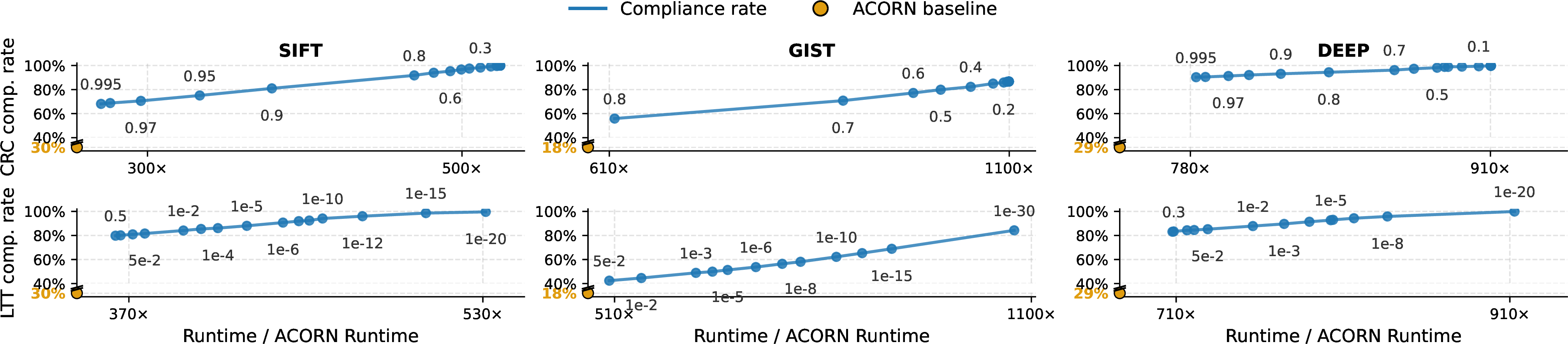
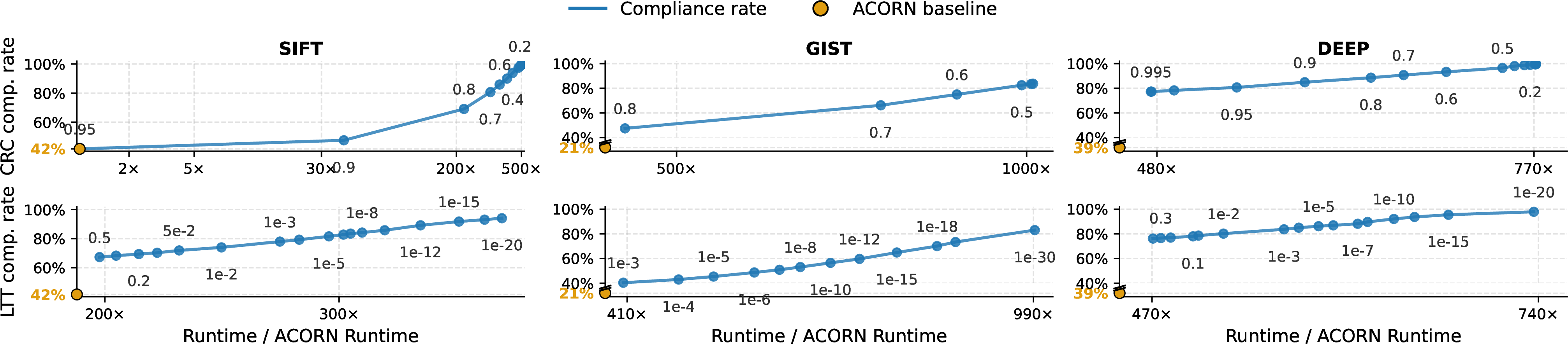


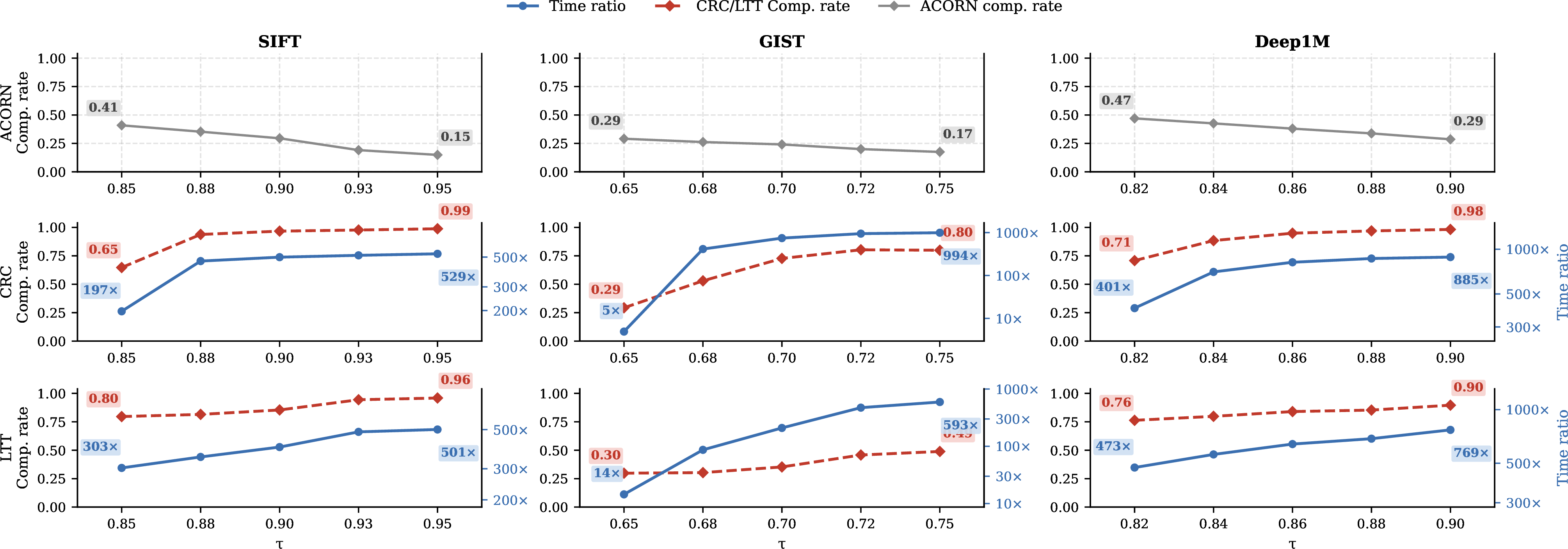
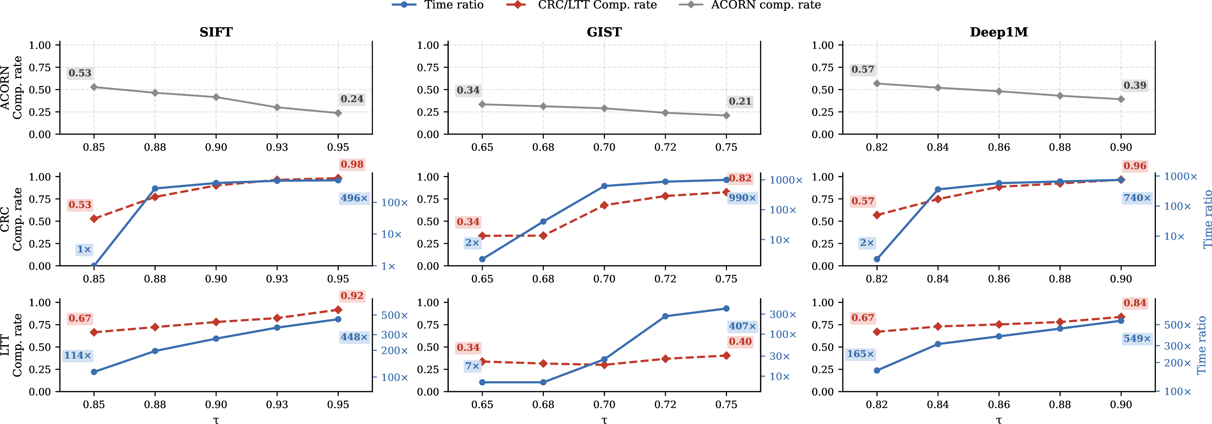
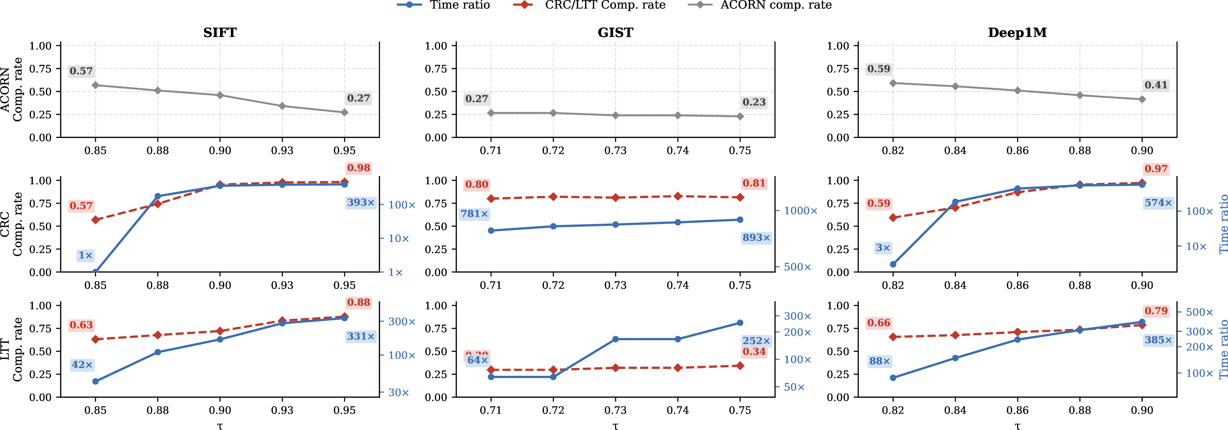

Effect of Varying \(\alpha\) (Alpha-Sweeps). The parameter \(\alpha\) governs the stringency of the statistical certifier. In CRC, \(\alpha\) controls the risk level of the conformal procedure: a smaller \(\alpha\) requires stronger statistical evidence that the HNSW output meets the recall target before it is accepted without rectification. In LTT, \(\alpha\) serves as the significance level of the hypothesis test that the certifier’s error rate does not exceed a prescribed tolerance \(\epsilon\).
Figures 18, 19 and 20 present the alpha-sweep results for selectivity levels \(\sigma = 5\), \(10\), and \(25\), respectively for datasets with synthetic predicates. Figure 21 presents alpha-sweep results for datasets with real query predicates. Each panel plots the compliance rate (y1 axis) and the normalized runtime (y2 axis) as a function of \(\alpha\), for both CRC and LTT. The baseline ACORN operating point is highlighted for reference.
For CRC, the results reveal a smooth and monotonic trade-off. At small values of \(\alpha\), the certifier is highly conservative: it demands strong statistical evidence before accepting ACORN results, so a large fraction of queries fail certification and are escalated to the exact F-SBE-Q + MBV recovery pipeline. This drives the compliance rate close to \(1.0\), where nearly every query ultimately meets the recall target, albeit at the cost of elevated runtime, since the Dijkstra-based expansion in F-SBE-Q is substantially more expensive than the heuristic traversal alone. As \(\alpha\) increases, the certifier becomes more permissive: it accepts a larger share of ACORN outputs at face value, bypassing rectification. This reduces runtime because fewer queries invoke the expensive recovery procedure, but the compliance rate decreases accordingly, since some of the directly accepted results do not actually meet the target recall.
For LTT, our results exhibit the same qualitative monotonic trade-off but with a notable quantitative difference: the practically useful range of \(\alpha\) in LTT is shifted toward substantially smaller values (often by many orders of magnitude). This is an inherent property of the Learn-then-Test mechanism rather than an indication of an unusually stringent confidence requirement. In LTT, the null hypothesis is the boundary case in which exactly \(x_\theta\) failures occur among \(m_\theta\) certified queries under a \(\text{Binomial}(m_\theta, \epsilon)\) model. The corresponding one-sided tail probability becomes extremely small as soon as the observed failure count drops even slightly below the nominal level \(\epsilon \cdot m_\theta\). As a result, the test rejects the null (and therefore certifies the query) only at very small \(\alpha\) values, compressing the effective operating range. Despite this shift, the shape of the compliance-versus-runtime frontier mirrors that of CRC: decreasing \(\alpha\) pushes more queries through rectification, raising both compliance and runtime, while increasing \(\alpha\) does the reverse.
Effect of Varying \(\tau\) (Tau-Sweeps). Figures 22, 23 and 24 present our results for tau-sweep experiments on datasets with synthetically generated predicates, while Figure 25 presents those for datasets with real predicates. In our experiments, we fix the certifier parameters and vary the target recall threshold \(\tau\). Each panel reports three quantities as a function of \(\tau\): the compliance rate of the CTR pipeline, the compliance rate of standalone ACORN without any certification or rectification, and the runtime ratio of the CTR pipeline relative to ACORN.
The results reveal a striking complementary pattern. As \(\tau\) increases (i.e., stricter recall requirements), ACORN’s native compliance rate declines steeply: at high recall thresholds, fewer and fewer of ACORN’s heuristic results happen to contain a sufficiently large overlap with the true \(k\)-nearest filtered neighbors. In contrast, the CTR pipeline maintains a substantially higher compliance rate across the full range of \(\tau\). This is because the certifier detects the queries for which ACORN’s output is deficient and escalates them to exact recovery via SBE-Q with MBV, which is guaranteed to return the true filtered neighbors. The gap between ACORN and CTR curves quantifies the value added by the certify-then-rectify mechanism: it is precisely those queries that would have silently returned low-recall results under ACORN alone that are caught and corrected. The runtime-ratio curve increases with \(\tau\), reflecting the fact that higher recall targets cause more queries to fail certification and require rectification. This increase is gradual at low-to-moderate \(\tau\) values (where ACORN already achieves reasonable recall for most queries) and steepens at high \(\tau\) values as the fraction of rectified queries grows.
Effect of Varying the Selectivity Parameter (\(\sigma\)). The alpha-sweep figures report runtime as a ratio relative to ACORN’s own runtime rather than as absolute latency. This normalization removes a large shared runtime component (the filtered traversal itself) and consequently compresses between-selectivity differences. In our experiments, ACORN’s absolute runtime is already fairly similar across selectivity levels (especially on SIFT1M), so the dominant visible variation within each panel comes from the \(\alpha\)-driven certification and rectification behavior rather than from \(\sigma\) directly.
Nevertheless, the effect of selectivity is discernible, particularly at the high-runtime end of the alpha frontier (i.e., at small \(\alpha\), where rectification is triggered most frequently). At this end, the runtime ratio decreases as selectivity decreases from \(\sigma = 5\) to \(\sigma = 25\). The mechanism is as follows: when the predicate is less selective (\(\sigma = 25\)), a larger fraction of the database satisfies the filter, so ACORN’s heuristic traversal is more likely to encounter qualifying candidates and return a result that already meets the recall target. Consequently, fewer queries require rectification, and the average per-query overhead shrinks. Conversely, at \(\sigma = 5\), the predicate is highly restrictive; ACORN must traverse deeper into the graph to find \(k\) qualifying neighbors, increasing the chance of a suboptimal result and triggering rectification more often. Thus, selectivity effects manifest primarily as vertical shifts in the runtime axis rather than as changes in the overall shape of the compliance curve.
Concluding Remarks. Taken together, these results validate that the Certify-then-Rectify framework transfers naturally to the filtered search setting. Across all datasets and across selectivity levels ranging from highly restrictive (\(\sigma = 5\)) to moderately selective (\(\sigma = 25\)), the CTR pipeline consistently achieves substantially higher compliance with the target recall than standalone ACORN, at a controlled and tunable runtime overhead. The \(\alpha\) parameter provides a smooth knob for navigating this trade-off: conservative settings (small \(\alpha\)) prioritize correctness, while permissive settings (large \(\alpha\)) prioritize speed. As part of future efforts, we plan to investigate how information about different predicates-including their distribution, cardinality, and proximity to the query point-can be exploited to further optimize the framework. In particular, we intend to study whether predicate-specific stretch values can reduce the overhead incurred during rectification for highly restrictive filters, and whether adaptive calibration strategies can improve the certifier’s discrimination when the predicate selectivity varies across queries within a single workload.
9 Related Work↩︎
A dominant family of graph indexing and ANN search algorithms stems from proximity-construction methods grounded in the geometry of relative neighborhood graphs (RNGs) and approximate Delaunay graphs [23], [24]. Key examples include navigable indexes such as Navigable Small-World graphs (NSW) and their hierarchical HNSW variant [1], [25], which constitute the state-of-the-art. Given its success, many variants of the vanilla HNSW have been proposed in recent literature [2], [26]–[28]. Related approaches further include navigating spread-out graphs (NSGs) [29] and the disk-based DiskANN index [13]. Efforts have also been made to accelerate kNN search by compressing the vector space using quantization [30] and inverted file (IVF) indexing [31], [32], and using locality-sensitive hashing [33]–[35]. A comprehensive survey on ANN search appears in [36]. For filtered search, the literature can be split into: (i) works on filter-aware index structures [26], [28], [37], [38]; (ii) standard ANN backbones with improved query-time execution [2], [39]; and (iii) multi-index approaches [40]. A survey of filtered search methods is given in [41].
Beyond improving the search algorithm itself, recent work has emphasized that query difficulty and workload composition strongly affect the observed behavior of ANN indexes. Wang et al. [42] introduced Steiner-hardness, a query hardness measure specifically designed for graph-based ANN indexes, while Ceccarello et al. [18] studied how to evaluate and generate query workloads of controlled difficulty for high-dimensional vector similarity search. Recent work further explores learned termination checks, where models map query-time features to per-query budgets [7], [43], [44]. Related declarative target-recall approaches terminate when the system predicts (heuristically) that the target recall has been met (e.g., DARTH [3]). Similar early-exit ideas also appear in non-graph pipelines [20], [45]–[48]. We also build on statistical models grounded in extreme value theory, including standard inferential toolkits for Weibull distributions [49], [50] and conformal prediction [14]–[16], [51]. Lastly, note that our formulations w.r.t. distance-call pruning take inspiration from recent literature on this topic [44], [52]–[59].
10 Final Remarks↩︎
This paper introduces a framework for generating correctness certificates in ANN search by wrapping HNSW in a "Certify-then-Rectify" pipeline. Using a Conformal Prediction formulation, we efficiently certify whether HNSW’s top-k results miss closer neighbors. If certification fails, we trigger exact recovery to fetch true top-k neighbors. Our key novelty is reinterpreting HNSW’s bottom layer as an empirical graph spanner to estimate a high-confidence stretch factor, bounding the exact recovery search radius. Recovery uses Stretch-Bounded Expansion from Query (SBE-Q) and Metric Bound Verification (MBV) to prune distance computations while preserving correctness. The framework supports filtered search without predicate-respecting paths.
References↩︎
In the sequel we use the term exact search when deploying MBV, with the understanding that the probability to identify the true kNN can be made arbitrarily high as per Section 6.4 evaluated further empirically in Section 7.↩︎
Both SIFT1M and GIST1M from: http://corpus-texmex.irisa.fr/↩︎
Both DEEP and T2I from: https://research.yandex.com↩︎
Vanilla HNSW has no guarantee in connectivity (see also [2]). Our stretch calculation is therefore conducted only for reachable nodes, despite unreachable nodes being rare (3 \(in\;degree{=}0\) nodes in our SIFT1M \(M{=}16,efc{=}200\) graph).↩︎
In our technical report [19] we explore repeating certification attempts with an expanded search radius to maintain compliance and mitigate runtime increases↩︎
https://research.yandex.com/blog/benchmarks-for-billion-scale-similarity-search↩︎
https://huggingface.co/datasets/SPCL/arxiv-for-fanns-large↩︎