1 Introduction↩︎

Finite-strain elasticity provides the framework for a wide spectrum of materials and applications in which the assumption of infinitesimally small displacements is no longer tenable [1], [2]. Once large deformations enter, the linear relation between stress and strain of Hooke’s law is lost and the governing equations become nonlinear, both geometrically and, in general, materially [3]. Since analytical solutions for such problems are rarely available, one relies on numerical methods, primarily the Finite Element Method (FEM), which discretises the weak (or, for hyperelastic materials, the variational) formulation of the problem [4], [5]. Two practical difficulties, however, persistently accompany finite element simulations at finite strain: the treatment of complex geometries, and the consistent derivation of the linearised operators required by Newton-type solvers. This paper addresses both within a single variational framework.

In classical, body-fitted FEM the mesh matches the geometry of the domain, so that the overall complexity of a simulation is concentrated in the meshing procedure [6], which becomes expensive for intricate or evolving geometries [7]. Non-matching (unfitted, immersed) methods avoid this bottleneck by embedding the physical domain into a fixed background mesh and describing its boundary implicitly, typically by a level-set function [8]. The family of such methods includes the Partition of Unity FEM [9], the Extended/Generalised FEM [10], [11], the Immersed FEM [12], the Shifted Boundary Method [13], and the Cut Finite Element Method (CutFEM), introduced in [14] and reviewed comprehensively in [8], [15]. In this work we adopt CutFEM in its classical form: Dirichlet boundary conditions are imposed weakly by Nitsche’s method [16], closely related to stabilised Lagrange multiplier formulations [17]–[19], and the small-cut ill-conditioning is cured by ghost-penalty stabilisation [20], [21].

Although CutFEM has matured rapidly, with applications ranging from linear elasticity [22], [23] to fluid–structure interaction [24]–[26] and contact problems [27]–[29], its application to nonlinear elasticity remains comparatively scarce. The principal contributions are [30]–[33], each presenting an unfitted discretisation of a finite-strain problem: [33] treats fracture and contact, [31] coupled mechanics–diffusion–reaction, [30] boundary-value and interface problems, and [32] elasto-plasticity with an aggregation-based alternative to the ghost penalty. All of these impose Dirichlet conditions weakly in the spirit of Nitsche, and [31], [33] derive residual and tangent from a total variational formulation. None of them, however, reports the use of automatic differentiation for the constitutive derivatives.

The second difficulty mentioned above is the derivation of the residual and tangent themselves. At finite strain these involve the first Piola–Kirchhoff stress tensor and the fourth-order elasticity tensor, i.e. the first and second derivatives of the strain energy density. Manual derivation is error-prone and its implementation cumbersome [34], while finite differences suffer from truncation errors; both jeopardise the consistent linearisation on which the quadratic convergence of Newton’s method depends [35]. Automatic differentiation (AD) offers an exact and flexible alternative: it computes derivatives of arbitrarily complex functions to machine precision, provided they decompose into elementary operations with known derivatives [36], [37]. Its use for residual and tangent generation in nonlinear solid mechanics has been demonstrated on fitted meshes [34], [37]–[39], and pairs naturally with energy-based formulations [40], [41]: once the material law is specified as an energy, residual and tangent follow mechanically by differentiation, and the code becomes model-independent.

In this paper we combine these ingredients into a single, fully variational CutFEM framework for nonlinear elasticity. The key structural observation is that not only the bulk material response, but also the Nitsche boundary terms and the ghost-penalty stabilisation can be incorporated into one augmented energy functional, from which the complete discrete residual and (symmetrised) tangent follow by successive variations. This energy formulation has immediate practical consequences: the tangent is symmetric by construction, the damped Newton iteration becomes a descent method for the total energy, and the constitutive derivatives (the Piola–Kirchhoff stress tensor and the fourth-order elasticity tensor) are generated by AD (here via AceGen, following [42]). Consequently, exchanging the hyperelastic model requires changing only the scalar energy density. To the best of our knowledge, no previous work combines (i) an unfitted finite element discretisation, (ii) nonlinear elasticity, (iii) automatic differentiation, and (iv) a model-independent, energy-only formulation in a single framework.

On the theoretical side, we analyse the linearised problem solved at each Newton step: we prove cut-independent coercivity, continuity, and an \(O(h^{-2})\) condition number bound under a uniform ellipticity assumption along the Newton path, and show that the damped Newton iteration is a descent method for the total energy. Verifying the three Brezzi–Rappaz–Raviart assumptions [43] for the linearised CutFEM forms (stability from the cut-independent coercivity, consistency from the interpolation estimate, and the Lipschitz tangent on the regular branch, in the sense of [43]) yields a quasi-optimal convergence theorem for regular (corner-free) solutions, with the symmetrised-tangent approximation accounted for through the exactly assembled residual. We then analyse the accuracy at unfitted Dirichlet–Neumann junctions, where the regularity that underpins this theorem fails. When such a junction lies in the interior of a cut cell, the corner singularity \(r^\lambda\) of the exact solution [44], [45] cannot be reproduced by a single polynomial on the junction cell, and we prove an unconditional lower bound that caps the \(L^2\) rate at \(h^{\min(p+1,\,2\lambda)}\) independently of the polynomial degree, the Nitsche parameter, the stabilisation, the quadrature, and, by the same regularity argument, the alignment of the junction with the background mesh. This cap is a property of the exact solution, shared with body-fitted discretisations on quasi-uniform meshes; what is specific to the unfitted setting is that none of its devices (exact junction quadrature, penalty tuning, vertex alignment) removes it. We quantify the dependence of \(\lambda\) on the material parameters via the Kolosov–Muskhelishvili characteristic equation, for both the clamped–free (mixed) and clamped–clamped corner: on a straight boundary segment the first-order cap is material-independent, while at a right-angle corner a smaller Poisson ratio mitigates but never removes the degradation for \(p \geq 2\). Finally, we show that the cap is removable by local mesh refinement and that the resulting rate is inherited by CutFEM cut-independently: whatever rate a matching mesh attains on the same background refinement, the unfitted discretisation attains too (Theorem 2,9). Consequently, the corner-specific analysis reduces to the classical body-fitted question.

We validate the framework on two hyperelastic models, the neo-Hookean model and a deviatoric–volumetric split neo-Hookean model, run through the identical code path with only the scalar energy density changed, directly demonstrating the model-independence of the energy-only formulation. On a smooth, corner-free disc test case both models attain optimal \(h\)-convergence for \(p = 1, 2, 3\). On the pole geometry we then exhibit the predicted corner behaviour: under mixed boundary conditions the Dirichlet–Neumann junctions cap the rate at \(2\lambda < 2\) for every polynomial degree, while under pure Dirichlet conditions the milder clamped–clamped corners cap it at \(2\lambda \in (2, 3.27)\), optimal only for \(p = 1\). Errors are measured against a matching body-fitted discretisation on the same meshes, and the singular-exponent predictions are confirmed across a sweep of the Poisson ratio in linear elasticity.

The remainder of the paper is a round trip from formulation to discretisation, through numerics, and back to analysis to understand and remedy the convergence cap that the numerics reveal at corners. Section 2 casts the finite-strain problem as energy minimisation and derives the residual and tangent driving the damped Newton scheme. Section 3 brings this to the CutFEM setting, covering level-set geometry, energy-consistent Nitsche boundary terms, ghost-penalty stabilisation, and AD-generated constitutive tensors. Section 4 establishes stability, conditioning, and convergence for the resulting linearised problems. Section 5 then verifies these predictions numerically: smooth domains behave exactly as theory promises, but corners introduce an unexpected accuracy cap. The remaining sections return to theoretical analysis to explain and remove it. Section 6 identifies the cap as an approximation-theoretic obstruction at unfitted Dirichlet–Neumann junctions and quantifies this effect through the Kolosov–Muskhelishvili characteristic equation, while Section 7 proposes local mesh grading as a remedy and confirms numerically that it restores optimal, cut-independent convergence rates; the supporting stability analysis is proved in 9.

2 Problem Formulation↩︎

We intend to solve problems in nonlinear elasticity whereby the material law is formulated as an energy functional. We begin by deriving the tangent and residual in the abstract sense, which are directly used in linearising the problem using Newton’s method. The presentation of the energy minimisation problem is synthesised from [46] and [47]. We follow the notation commonly used in solid mechanics literature (e.g., [46], [48], [49]), where \(\Delta \boldsymbol{U}\) and \(\Delta \boldsymbol{u}\) refer to the correction of the displacement field \(\boldsymbol{u}\) rather than the Laplacian operator.

Many problems in elasticity lend themselves well to being formulated as minimisation problems of an energy functional [5]. To make this energy functional explicit for elastic materials, we begin by introducing the basic kinematic quantities that characterise the deformation of the body. A hyperelastic material has both a reference configuration and a current configuration. One may liken this to a ground state and a deformed state. We define the domain of the current configuration as \(\omega\), which is linked to the reference domain \(\Omega \subset \mathbb{R}^d\) by the deformation mapping \(\boldsymbol{\varphi} : \Omega \rightarrow \mathbb{R}^d\). We use the mapping to define the displacement field \(\boldsymbol{u}\) as the difference between the position in the reference and current configurations. In other words, given a position vector \(\boldsymbol{X} \in \Omega\), and the resulting location \(\boldsymbol{x} \in \omega\): \[\begin{align} \boldsymbol{u}(\boldsymbol{X}) & = \boldsymbol{\varphi}(\boldsymbol{X}) - \boldsymbol{X} \\ & = \boldsymbol{x} - \boldsymbol{X} \end{align}\] This can then be used to define the deformation gradient \(\boldsymbol{F}\), which is one of the kinematic quantities of primary interest. The deformation gradient \(\boldsymbol{F}\) has a few common alternative notations, namely: \[\boldsymbol{F} = \frac{\partial \boldsymbol{x}}{\partial \boldsymbol{X}} = \frac{\partial \boldsymbol{\varphi}}{\partial \boldsymbol{X}} = \nabla\boldsymbol{\varphi} = \boldsymbol{I} + \nabla\boldsymbol{u}\] where \(\nabla(\cdot)\) denotes the gradient in the reference configuration. This deformation gradient \(\boldsymbol{F}\) is then used to define the energy functional \(\mathcal{E}(\boldsymbol{u})\). In elasticity, one will typically see \(\mathcal{E}(\boldsymbol{u})\) being defined in terms of \(\boldsymbol{F}\):

\[\label{eq:energy} \mathcal{E}(\boldsymbol{u}) := \int_\Omega \Psi(\boldsymbol{F}) \:\: d V - \int_\Omega \boldsymbol{f}_0\cdot \boldsymbol{u} \:\: d V - \int_{\Gamma_N} \boldsymbol{t}_0 \cdot \boldsymbol{u} \:\: d S\tag{1}\] where \(\Psi(\boldsymbol{F})\) is the strain energy density function, which describes the elastic response of the material, \(\boldsymbol{f}_0\) describes internal body forces, and \(\boldsymbol{t}_0\) describes the surface traction applied on the Neumann boundary \(\Gamma_N \subset \partial \Omega\) [47]. In contrast to the Dirichlet boundary, where \(\boldsymbol{u}\) is fixed, on the Neumann boundary surface tractions are applied. Since the energy is formulated in the reference configuration, the applied traction is given by \(\boldsymbol{t}_0 = \boldsymbol{P}\boldsymbol{N}\), where \(\boldsymbol{P}\) is the first Piola–Kirchhoff stress tensor introduced below and \(\boldsymbol{N}\) is the outward unit normal in the reference configuration [47].

Given a space of admissible displacements \(U\), the energy minimisation problems require that we seek a \(\boldsymbol{u} \in U\) s.t.: \[\label{eq:energyminimisationproblem} \mathcal{E}(\boldsymbol{u}) = \text{inf}_{\boldsymbol{v} \in U} \mathcal{E}(\boldsymbol{v})\tag{2}\] which can be found by setting the first variation of 1 equal to 0. In the context of finite-strain elasticity, this minimum point refers to where the material is in a state of equilibrium [47]. In this setting, the first variation, which we refer to as the nonlinear residual function, is equal to the Gateaux derivative of \(\mathcal{E}\) at the current iterate \(\bar{\boldsymbol{u}}\) in a direction \(\delta \boldsymbol{u}\), which represents an infinitesimal perturbation to \(\bar{\boldsymbol{u}}\). The Gateaux derivative \(D_{\delta\boldsymbol{u}}\mathcal{E}(\bar{\boldsymbol{u}})\) looks as follows: \[\begin{align} \label{nonlinres} D_{\delta\boldsymbol{u}}\mathcal{E}(\bar{\boldsymbol{u}}) := \mathcal{F}(\bar{\boldsymbol{u}}, \delta\boldsymbol{u}) & = \int_\Omega \frac{\partial \Psi}{\partial \nabla\: \boldsymbol{u}}\bigg|_{\bar{\boldsymbol{u}}}: \nabla\delta \boldsymbol{u} \: dV - \int_\Omega \boldsymbol{f}_0\cdot \delta\boldsymbol{u} \:\: d V - \int_{\Gamma_N} \boldsymbol{t}_0 \cdot \delta\boldsymbol{u} \:\: d S \\ & = \int_\Omega \boldsymbol{P} : \nabla\delta\boldsymbol{u} \:\: d V - \int_\Omega \boldsymbol{f}_0\cdot \delta \boldsymbol{u} \:\: d V - \int_{\Gamma_N} \boldsymbol{t}_0 \cdot \delta \boldsymbol{u} \:\: d S \end{align}\tag{3}\] where \(\boldsymbol{P}\) is the Piola–Kirchhoff tensor: \[\boldsymbol{P}:=\frac{\partial\Psi }{\partial\boldsymbol{F}}= \frac{\partial\Psi}{\partial \boldsymbol{\text{ Grad } u}}\] and so the problem becomes \[\int_\Omega \boldsymbol{P} : \text{ Grad }\delta\boldsymbol{u} \:\: d V - \int_\Omega \boldsymbol{f}_0\cdot \delta \boldsymbol{u} \:\: d V - \int_{\Gamma_N} \boldsymbol{t}_0 \cdot \delta \boldsymbol{u} \:\: d S = 0 \:\: \forall \delta \boldsymbol{u}\] We define the tangent operator: \[\begin{align} \label{eq:tangent} \mathcal{K}(\bar{\boldsymbol{u}}, \Delta \boldsymbol{u}, \delta \boldsymbol{u}) & := D_{\Delta\boldsymbol{u}}\mathcal{F}(\bar{\boldsymbol{u}}, \delta \boldsymbol{u}) \\ & = \int_\Omega D_{\Delta\boldsymbol{u}}\boldsymbol{P} : \nabla \delta\boldsymbol{u} \; d V = \int_\Omega \nabla\Delta\boldsymbol{u} : \mathbb{L} : \nabla\delta\boldsymbol{u} \; d V , \end{align}\tag{4}\] with the fourth-order tensor \(\mathbb{L}\): \[\label{eq:L} \mathbb{L} := \frac{\partial\boldsymbol{P}}{\partial\boldsymbol{F}} = \frac{\partial^2\Psi}{\partial\boldsymbol{F}\otimes\partial\boldsymbol{F}} .\tag{5}\] which requires the calculation of the tensor product (denoted \(\otimes\)) of two second-order tensors and possesses the major symmetry \(L_{ijkl} =L_{klij}\).

Starting from the energy \(\mathcal{E}(\boldsymbol{u})\) as defined in 1 , we obtain the following variational formulation: \[\begin{align} \mathcal{F}(\bar{\boldsymbol{u}}, \delta\boldsymbol{u}) & := D_{\delta \boldsymbol{u}}\mathcal{E}(\bar{\boldsymbol{u}}) \\ & = \int_\Omega \boldsymbol{P} : \nabla\delta\boldsymbol{u} \: d V - \int_\Omega \boldsymbol{f}_0\cdot \delta\boldsymbol{u} \:\: d V -\int_{\Gamma_N} \boldsymbol{t}_0 \cdot \delta \boldsymbol{u} \:\: d S = 0 \:\: \forall \delta \boldsymbol{u} \\ \mathcal{K}(\bar{\boldsymbol{u}}, \Delta \boldsymbol{u}, \delta \boldsymbol{u}) & := D_{\Delta\boldsymbol{u}}\mathcal{F}(\bar{\boldsymbol{u}}, \delta \boldsymbol{u}) \\ & = \int_\Omega D_{\Delta\boldsymbol{u}}\boldsymbol{P} : \nabla \delta\boldsymbol{u} \; d V = \int_\Omega \nabla\Delta\boldsymbol{u} : \mathbb{L} : \nabla\delta\boldsymbol{u} \; d V \end{align}\]

2.1 Solving the Linearised Problem↩︎

The nonlinear residual function as defined in 3 is linear in \(\delta \boldsymbol{u}\), but generally nonlinear in \(\bar{\boldsymbol{u}}\). As a result, we rely on iterative methods to find the solution. A standard approach would be the Newton-Raphson method. In this method, a correction \(\Delta\boldsymbol{u}\) to the current approximation \(\boldsymbol{\bar{u}}\) is calculated by linearising the residual around \(\boldsymbol{\bar{u}}\): \[\mathcal{F}(\bar{\boldsymbol{u}}+\Delta\boldsymbol{u},\delta\boldsymbol{u}) \approx \mathcal{F}(\bar{\boldsymbol{u}},\delta\boldsymbol{u}) + \mathcal{K}(\bar{\boldsymbol{u}};\Delta\boldsymbol{u},\delta\boldsymbol{u}) = 0 \qquad \forall \delta \boldsymbol{u}\] which gives us Newton’s method update \(\Delta \boldsymbol{u}\) by solving the linear problem: \[\begin{align} \mathcal{K}(\bar{\boldsymbol{u}}; \Delta\boldsymbol{u}, \delta\boldsymbol{u}) & = -\mathcal{F}(\bar{\boldsymbol{u}}, \delta\boldsymbol{u}) \text{ for } \Delta\boldsymbol{u} \\ \label{eq:newtonupdate} \bar{\boldsymbol{u}}^{(k+1)} & = \bar{\boldsymbol{u}}^{(k)} + \beta \Delta\boldsymbol{u} \end{align}\tag{6}\] The parameter \(\beta\) denotes step-size control. Implementations of Newton’s method where \(0 < \beta < 1\) are often referred to as damped or relaxed Newton’s method. Relaxing \(\beta\) can prevent issues such as entrapment in local minima. A typical convergence criterion for the Newton-Raphson iteration would be when the residual norm \(||\mathcal{F}(\bar{\boldsymbol{u}}^{(k)}, \delta\boldsymbol{u}) ||\) falls below some tolerance threshold.

3 Discretisation with the Cut Finite Element Method↩︎

To solve the infinite-dimensional problem, the Finite Element Method (FEM) constructs a finite-dimensional subspace \(\mathbb{V}_h \subset \mathbb{V}\) and searches for a discrete solution \(\boldsymbol{u}_h \in \mathbb{V}_h\) such that \(\mathcal{F}(\boldsymbol{u}_h; \boldsymbol{v}_h) = 0\) for all discrete test functions \(\boldsymbol{v}_h \in \mathbb{V}_h\). The discrete solution \(\boldsymbol{u}_h\) is described as a linear combination of basis functions \(\{\varphi_j\}_{j=1}^N\) with coefficients \(\{U_j\}_{j=1}^N\), where \(N\) equals the number of degrees of freedom and \(\boldsymbol{U} = \{U_1, ..., U_N\}^T\) is the vector of unknown coefficients.

Typically, these basis functions are piecewise polynomial functions. More concretely, one defines a triangulation \(\mathcal{T}_h\), which divides the domain \(\Omega\) into simplices, for example triangles in 2D or tetrahedra in 3D. Each such simplex is called an element, and its finite element space is spanned by a polynomial space \(\mathcal{P}_K\). The basis functions \(\{\varphi_1, \varphi_2, ... , \varphi_N\}\) that span \(\mathcal{P}_K\) are used to calculate the integral on \(K\).

Finally, we look at the continuity requirements placed on these basis functions. Let \(L^2\) be the set of functions that are square-integrable ([50], page 91) and \(H^1(\Omega)\) the set of functions \(\in L^2\) whose weak derivatives exist and are also \(\in L^2\) (see [50], page 202). We seek a solution \(\boldsymbol{u}\) in the discretised space of vector-valued finite element functions for a \(d\)-dimensional problem: \[\mathbb{V}_h = \{\boldsymbol{u} \in \big(H^1(\Omega)\big)^d \:\:\: | \;\; \boldsymbol{u}_{|_K} \in \left(\mathcal{P}_K\right)^d \:\:\;\forall K \in \mathcal{T}^h \}.\] The sections that follow detail specific implementation details.

3.1 Non-Matching Mesh↩︎

In classical FEM, the mesh \(\mathcal{T}_h\) matches the domain \(\Omega\). In other words, the mesh is generated such that it coincides exactly with the geometry of the domain. In non-matching methods, however, the mesh is generated independently of the geometry. In order to make this notion more concrete, we introduce a level-set function \(\psi : \mathbb{R}^{d} \rightarrow \mathbb{R}\) that describes the geometry: \[\begin{align} \Omega & = \{x \in \mathbb{R}^{d}\: : \:\psi(x) < 0\} \\ \partial\Omega & = \{x \in \mathbb{R}^{d}\: : \:\psi(x) = 0\} \\ (\Omega \cup \partial\Omega )^c & = \{x \in \mathbb{R}^{d} \:: \:\psi(x) > 0\} \end{align}\] Let \(\mathcal{T}^h\) represent the independently-generated background mesh where our true domain \(\Omega\) rests, i.e., \(\Omega \subset \bigcup_{T \in \mathcal{T}^h} T\). Figure 1 illustrates an example of a uniform background mesh and a domain boundary. This level-set description allows us to classify each cell of the mesh as being interior (\(K \subset \Omega\)), exterior (\(K \cap \Omega = \emptyset\)), or cut (\(K \cap \partial\Omega \neq \emptyset\)). We define two subsets of the background mesh: the active mesh \(T_\Omega^h = \{T \in \mathcal{T}^h : T \cap \Omega \neq \emptyset\}\) and the set of cut cells \(T_{\partial\Omega}^h = \{T \in T_\Omega^h : T \cap \partial\Omega \neq \emptyset\}\).

3.2 Boundary Conditions↩︎

Due to the non-matching nature of the mesh, in CutFEM it is not possible to directly impose boundary conditions. Instead, the method uses Nitsche’s method of weakly imposing boundary conditions, first proposed in [16]. Weakly imposing the boundary conditions results in three additional terms to the overall tangent and residual, which serve the purpose of restoring (i) consistency, (ii) coercivity and (iii) symmetry [52]. These are central properties that ensure well-posedness and stability of elliptic partial differential equations, see for example Cea’s lemma, Riesz’ representation theorem and the Lax-Milgram lemma.

Rather than postulating the Nitsche terms directly at the level of the residual and tangent, we derive them from an augmented energy functional, consistently with the variational framework of Section 2. For homogeneous Dirichlet conditions on \(\partial\Omega\), we define \[\label{eq:nitscheenergy} \mathcal{E}_{h}(\boldsymbol{u}) := \mathcal{E}(\boldsymbol{u}) - \int_{\partial\Omega} \boldsymbol{n} \cdot \boldsymbol{P}(\boldsymbol{u}) \cdot \boldsymbol{u} \: dS + \int_{\partial\Omega} \frac{\gamma_D \, \eta(\bar{\boldsymbol{u}})}{2h} \, |\boldsymbol{u}|^2 \: dS ,\tag{7}\] where the first boundary term restores consistency (it is the work of the boundary traction \(\boldsymbol{P}\boldsymbol{n}\), which does not vanish on the unfitted boundary) and the second is a quadratic penalty enforcing coercivity, with a stiffness weight \(\eta(\bar{\boldsymbol{u}})\) (defined in 12 below) that is evaluated at the current iterate and held fixed when taking variations. Taking the first variation of the boundary terms in 7 in a direction \(\boldsymbol{v}_h\) yields the boundary contribution to the residual: \[\begin{align} \label{eq:fbound} \mathcal{F}_{\text{Bound}}(\boldsymbol{\bar{u}}, \boldsymbol{v}_h) & = -\mathcal{F}_{\text{Nonlinear}}(\boldsymbol{\bar{u}}, \boldsymbol{v}_h) - \mathcal{F}_{\text{Linear}}(\boldsymbol{\bar{u}}, \boldsymbol{v}_h) + \mathcal{F}_{\text{Penalty}}(\boldsymbol{\bar{u}}, \boldsymbol{v}_h) \end{align}\tag{8}\] with \[\begin{align} \tag{9} \mathcal{F}_{\text{Nonlinear}}(\boldsymbol{\bar{u}}, \boldsymbol{v}_h) & = \int_{\partial \Omega} \boldsymbol{n} \cdot \boldsymbol{P}(\bar{\boldsymbol{u}})\cdot \boldsymbol{v}_h \: dS \\ \tag{10} \mathcal{F}_{\text{Linear}} (\boldsymbol{\bar{u}}, \boldsymbol{v}_h) & = \int_{\partial \Omega} \boldsymbol{n} \cdot (\mathbb{L}(\boldsymbol{\bar{u}}) : \nabla\boldsymbol{v}_h) \cdot \bar{\boldsymbol{u}} \: dS \\ \mathcal{F}_{\text{Penalty}}(\boldsymbol{\bar{u}}, \boldsymbol{v}_h) & = \int_{\partial \Omega}\frac{\gamma_D \, \eta(\bar{\boldsymbol{u}})}{h}\bar{\boldsymbol{u}}\cdot \boldsymbol{v}_h\:dS \end{align}\] The term 9 arises from varying \(\boldsymbol{u}\) in the second slot of the consistency term in 7 and is a direct consequence of the natural boundary condition \(\boldsymbol{P}\boldsymbol{n} = \boldsymbol{t}_0\) (see the term defined on \(\Gamma_N\) in 1 ); the term 10 arises from varying the stress, \(D_{\boldsymbol{v}_h}\boldsymbol{P} = \mathbb{L} : \nabla\boldsymbol{v}_h\), and restores symmetry; the factor \(1/2\) in the penalty energy of 7 is cancelled automatically by differentiating the quadratic penalty. The terms \(\mathcal{F}_{\text{Nonlinear}}\) and \(\mathcal{F}_{\text{Linear}}\) coincide with the formulation of [33] (eq. 28), which defines the weak nonlinear residual: the second term of eq. 28 in [33] considers the full nonlinear stress, and the third term considers the stress linearised around the current iterate. The key difference is that the definition in [33] applies to a contact problem, and therefore considers displacement gaps \([[\boldsymbol{u}]]\) across an interface. In our formulation, the “interface” is the boundary \(\partial\Omega\), and we weakly enforce homogeneous Dirichlet boundary conditions, and so \([[\boldsymbol{u}]]\) simplifies to \(\bar{\boldsymbol{u}}\). The penalty term \(\mathcal{F}_{\text{Penalty}}\) is analogous to the residual penalty terms in [32] and [33].

Differentiating \(\mathcal{F}_{\text{Bound}}\) once more in the direction \(\boldsymbol{u}_h\) yields the boundary contribution to the tangent: \[\begin{align} \label{eq:kbound} \mathcal{K}_{\text{Bound}}(\boldsymbol{\bar{u}}; \boldsymbol{u}_h, \boldsymbol{v}_h) = & -\mathcal{K}_{\text{Const}}(\boldsymbol{\bar{u}}; \boldsymbol{u}_h, \boldsymbol{v}_h) -\mathcal{K}_{\text{Symm}}(\boldsymbol{\bar{u}}; \boldsymbol{u}_h, \boldsymbol{v}_h) + \mathcal{K}_{\text{Penalty}}(\boldsymbol{\bar{u}}; \boldsymbol{u}_h, \boldsymbol{v}_h) \end{align}\tag{11}\] with \[\begin{align} \mathcal{K}_{\text{Const}}(\boldsymbol{\bar{u}}; \boldsymbol{u}_h, \boldsymbol{v}_h) & = \int_{\partial\Omega} \boldsymbol{n} \cdot (\mathbb{L}(\boldsymbol{\bar{u}}) : \nabla\boldsymbol{u}_h)\cdot \boldsymbol{v}_h \: dS \\ \mathcal{K}_{\text{Symm}}(\boldsymbol{\bar{u}}; \boldsymbol{u}_h, \boldsymbol{v}_h) & = \int_{\partial \Omega} \boldsymbol{n} \cdot (\mathbb{L}(\boldsymbol{\bar{u}}) : \nabla\boldsymbol{v}_h)\cdot \boldsymbol{u}_h \: dS \\ \mathcal{K}_{\text{Penalty}}(\boldsymbol{\bar{u}}; \boldsymbol{u}_h, \boldsymbol{v}_h) & = \int_{\partial \Omega}\frac{\gamma_D \, \eta(\bar{\boldsymbol{u}})}{h}\boldsymbol{u}_h\cdot \boldsymbol{v}_h\:dS \end{align}\] The terms \(\mathcal{K}_{\text{Const}}\) and \(\mathcal{K}_{\text{Symm}}\), formulated in terms of the linearised stress, are analogous to the formulations in [32] (eq. 8), [22] (eq. 21) and [53] (eq. 22). Although [22] and [53] formulate the terms for linear elasticity, they are fundamentally the same. There is, however, an important difference: the aforementioned papers both consider a constant elasticity tensor, but in the nonlinear case, the linearised stress must be evaluated at the current iterate, as it changes each iteration. The term \(\mathcal{K}_\text{Penalty}\) is analogous to the tangent penalty terms seen in [32], [27] and [53].

3.2.0.1 Remark (symmetrised tangent)

The exact second variation of 7 contains one additional term, \(-\int_{\partial\Omega} \boldsymbol{n} \cdot \big( (D_{\Delta\boldsymbol{u}}\mathbb{L}) : \nabla\boldsymbol{v}_h \big) \cdot \bar{\boldsymbol{u}} \: dS\), which involves the third derivative of the strain energy \(\Psi\). We omit this term from \(\mathcal{K}_{\text{Bound}}\) in 11 . This is the symmetrised approximation of the tangent: the omitted term is proportional to the boundary value of \(\bar{\boldsymbol{u}}\) and therefore vanishes as the iterates approach the solution of the weakly enforced homogeneous Dirichlet problem, so the consistency of the Newton scheme and the quadratic local convergence near the solution are unaffected, while the tangent retains its symmetry.

3.2.0.2 Remark (choice of penalty parameter)

The Nitsche parameter \(\gamma_D = 5(p+1)p\) is chosen to be large enough to enforce coercivity [22]; this is similar to the penalty parameter of \(5p^2\) as seen in [53]. The stiffness weight \(\eta\) is chosen adaptively at each boundary quadrature point as \[\label{eq:penaltyweight} \eta(\bar{\boldsymbol{u}}) := \max\left\{ 2\mu_e , \; \tfrac{1}{2}\,\|\mathbb{L}(\bar{\boldsymbol{u}})\|_1 \right\}, \qquad \|\mathbb{L}\|_1 := \sum_{i,j,k,l} |L_{ijkl}| ,\tag{12}\] where \(\mu_e\) denotes the shear modulus. In the small-strain regime \(\|\mathbb{L}(\bar{\boldsymbol{u}})\| \sim E\) and the weight reduces to the familiar shear-modulus scaling \(2\mu_e\); for the linear-elastic model \(\eta = 2\mu_e\). At finite strain the local stiffness is governed by the linearised elasticity tensor \(\mathbb{L}(\bar{\boldsymbol{u}})\), which may differ substantially from its small-strain limit, and coercivity of the linearised problem formally requires the penalty to dominate an inverse-trace constant scaled by \(\|\mathbb{L}(\bar{\boldsymbol{u}})\|\); the \(\|\mathbb{L}\|_1\)-based bound in 12 maintains this domination along the Newton path (cf. Proposition 1). Since \(\eta\) depends on \(\bar{\boldsymbol{u}}\), it is, like the consistency stress, frozen at the current iterate when taking variations; the neglected contribution is proportional to \(|\bar{\boldsymbol{u}}|^2\) on \(\partial\Omega\) and vanishes as the iterates approach the solution of the weakly enforced homogeneous Dirichlet problem, so the consistency and the local quadratic convergence of the Newton scheme are unaffected.

Hence, by using Nitsche’s formulation for weakly imposing the boundary condition, we do not remove permissible solutions from the Finite Element space, as we would when strongly imposing boundary conditions, but rather augment the energy by two boundary terms, whose first and (approximate) second variations enter the residual and tangent.

3.3 Ghost Penalty Stabilisation↩︎

A possible problem in CutFEM is that the system matrix may become ill-conditioned as a result of the small cut problem. This arises when, given an intersected cell \(K\), the volume of \(K \cap \Omega\) is very small compared to its overall volume, i.e. \(K \cap \Omega \ll h^d\) [53]. As a result, the support of the basis function defined over \(K\) is very small, leading to very small entries in the local stiffness matrix, thus resulting in an ill-conditioned matrix leading to a system that may converge very slowly, or not at all. To remedy this, an extra stabilisation term \(\mathcal{K}_{\text{Stab}}\) is added to the overall tangent operator. The particular stabilisation method used in this work is the ghost penalty, which was introduced in [20]. The objective of the ghost penalty is to reduce the discontinuity of functions or its (higher-order) derivatives for cut cells. Essentially, \(\mathcal{K}_{\text{Stab}}\) penalises the jump, or discontinuity, of the derivatives across the cut boundary. This type of “face” ghost penalty stabilisation enforces full \(C^m\) continuity in the limit \(\gamma_A \rightarrow \infty\) [54]. The formulae and explanations presented here are based on [55] and [51].

Figure 1 illustrates two categories of cells: those that are entirely inside the domain \(\Omega_h\), and those that are intersected by the boundary \(\partial \Omega_h\). For a given face \(F\) we distinguish between \(T^+\), a neighbouring element that is intersected by the boundary, and \(T^-\), an element that lies entirely in the domain. We use this to define \(\mathcal{F}_h\), the set of faces for which we calculate the penalty: \[\mathcal{F}_h = \{F = \overline{T}_+ \cap \overline{T}_- \: : \:T_+ \in \mathcal{T}_{\partial\Omega}^h, \: T_- \in \mathcal{T}_\Omega^h\}\] Using these definitions and concepts, we can define the ghost penalty terms for the tangent and residual: \[\begin{align} \tag{13} \mathcal{K}_{\text{Stab}}(\bar{\boldsymbol{u}}; \boldsymbol{u}_h, \boldsymbol{v}_h) & = \gamma_A \sum_{F \in \mathcal{F}_h} g_F(\boldsymbol{u}_h, \boldsymbol{v}_h) \\ \tag{14} \mathcal{F}_{\text{Stab}}(\bar{\boldsymbol{u}}, \boldsymbol{v}_h) & = \gamma_A \sum_{F \in \mathcal{F}_h} g_F(\bar{\boldsymbol{u}}, \boldsymbol{v}_h) \end{align}\] where \(\gamma_A = \alpha E\) is an additional stabilisation written in terms of the material’s Young’s modulus \(E\) and and \(g_F(\boldsymbol{u}_h, \boldsymbol{v}_h)\), the ghost penalty for a single face, is defined using the jump in derivatives, i.e: \[\begin{align} \label{ghost} g_F(\boldsymbol{u}_h, \boldsymbol{v}_h) & = \sum_{k=1}^p \left(\frac{h_F^{2k-1}}{(k!)^2}[\partial_n^k\boldsymbol{u}_h], [\partial_n^k\boldsymbol{v}_h]\right) _F \\ \notag & = \sum_{k=1}^p \left(\frac{h_F^{2k-1}}{(k!)^2} \int_F (\partial_n^k\boldsymbol{u}_h|_{\overline{T}_+} - \partial_n^k\boldsymbol{u}_h|_{\overline{T}_-})\cdot(\partial_n^k\boldsymbol{v}_h|_{\overline{T}_+} - \partial_n^k\boldsymbol{v}_h|_{\overline{T}_-})ds\right) \end{align}\tag{15}\] In penalising the jump in derivatives, the piecewise polynomial over \(\overline{T}_+ \cup \overline{T}_-\) is weakly enforced to behave as a single polynomial [55].

Like the Nitsche terms of the previous section, the stabilisation terms admit an energy interpretation: defining the stabilisation energy \[\label{eq:gpenergy} \mathcal{E}_{\text{Stab}}(\boldsymbol{u}) := \frac{\gamma_A}{2} \sum_{F \in \mathcal{F}_h} g_F(\boldsymbol{u}, \boldsymbol{u}),\tag{16}\] and noting that \(g_F\) is a symmetric bilinear form, 14 and 13 are exactly its first and second variations. The discrete problem is thus, in its entirety, the stationarity condition of a single augmented energy functional.

For Cartesian meshes, the ghost penalty evaluation can exploit the tensor product structure of the shape functions. The decomposition into 1D operators for scalar problems is described in [51]. For vector-valued problems, the ghost penalty is applied component-wise, resulting in a block-diagonal local stabilisation matrix for each face \(F\): \[\mathcal{K}_{\text{Stab}, F}^{\text{loc}} = \begin{pmatrix} \mathcal{G}_F & 0 & 0 \\ 0 & \mathcal{G}_F & 0 \\ 0 & 0 & \mathcal{G}_F \end{pmatrix},\] where each block exhibits a Kronecker product structure, e.g., \(\mathcal{G}_F = M^h \otimes M^h \otimes G^h_k\) in 3D. Since the 1D mass matrix \(M^h\) and 1D penalty matrix \(G^h_k\) are independent of the element location on a uniform grid, they are precomputed and stored to reduce assembly time.

3.4 Automatic Differentiation↩︎

Computing higher-order derivatives such as those often seen in the Jacobian matrices of nonlinear problems is a time-consuming and error-prone task [37]. Therefore, this work uses automatic differentiation to calculate the Piola–Kirchhoff tensor \(\boldsymbol{P}\) and fourth-order tensor \(\mathbb{L}\): \[\label{tensors} \boldsymbol{P}:=\frac{\partial\Psi }{\partial\boldsymbol{F}}= \frac{\partial\Psi}{\partial \boldsymbol{\text{ Grad } u}}; \qquad \mathbb{L} := \frac{\partial\boldsymbol{P}}{\partial\boldsymbol{F}} = \frac{\partial^2\Psi}{\partial\boldsymbol{F}\otimes\partial\boldsymbol{F}}\tag{17}\] We use the material parameters \(E\) (Young’s modulus) and \(\nu\) (Poisson’s ratio) when deriving the contributions \(\boldsymbol{P}\) and \(\mathbb{L}\) to the residual and tangent. Young’s modulus is a measure of the material’s stiffness, and Poisson’s ratio is the ratio between transverse and axial strain. The automatic differentiation is implemented in mathematica using AceGen using the code following [42].

3.5 Discretisation and Algorithm Summary↩︎

Collecting the contributions of the previous sections, the discrete problem is the stationarity condition of the total augmented energy \[\label{eq:totalenergy} \mathcal{E}_{\text{Total}}(\boldsymbol{u}_h) := \mathcal{E}(\boldsymbol{u}_h) - \int_{\partial\Omega} \boldsymbol{n} \cdot \boldsymbol{P}(\boldsymbol{u}_h) \cdot \boldsymbol{u}_h \: dS + \int_{\partial\Omega} \frac{\gamma_D \, \eta(\bar{\boldsymbol{u}})}{2h} \, |\boldsymbol{u}_h|^2 \: dS + \mathcal{E}_{\text{Stab}}(\boldsymbol{u}_h),\tag{18}\] combining 1 , 7 and 16 , with the penalty weight \(\eta\) frozen at the current iterate \(\bar{\boldsymbol{u}}\). The total residual is its first variation, and the total tangent is its second variation up to the omitted third-derivative boundary term and the frozen penalty weight discussed in Section 3.2; in particular, the tangent is symmetric by construction. The semi-discrete variational problem consists of finding \(\boldsymbol{u}_h \in V_h\) such that the total residual \(\mathcal{F}_{\text{Total}}(\bar{\boldsymbol{u}}, \boldsymbol{v}_h) = 0\) for all \(\boldsymbol{v}_h \in V_h\). We linearise this problem using a damped Newton-Raphson scheme. At each iteration \(k\), we solve for the correction \(\Delta \boldsymbol{U}\) in the linear system: \[(\mathbf{K}_{\Omega} + \mathbf{K}_{\text{Bound}} + \mathbf{K}_{\text{Stab}}) \Delta \boldsymbol{U} = -(\mathbf{F}_{\Omega} + \mathbf{F}_{\text{Bound}} + \mathbf{F}_{\text{Stab}})\] where \(\mathbf{K}\) and \(\mathbf{F}\) are the assembled matrices and vectors from the following bilinear and linear forms: \[\begin{align} \mathcal{K}_{\text{Total}}(\bar{\boldsymbol{u}}; \boldsymbol{u}_h, \boldsymbol{v}_h) & = \mathcal{K}_{\Omega}(\bar{\boldsymbol{u}}; \boldsymbol{u}_h, \boldsymbol{v}_h) + \mathcal{K}_{\text{Bound}}(\bar{\boldsymbol{u}}; \boldsymbol{u}_h, \boldsymbol{v}_h) + \mathcal{K}_{\text{Stab}}(\bar{\boldsymbol{u}}; \boldsymbol{u}_h, \boldsymbol{v}_h) \\ \mathcal{F}_{\text{Total}}(\bar{\boldsymbol{u}}, \boldsymbol{v}_h) & = \mathcal{F}_{\Omega}(\bar{\boldsymbol{u}}, \boldsymbol{v}_h) + \mathcal{F}_{\text{Bound}}(\bar{\boldsymbol{u}}, \boldsymbol{v}_h) + \mathcal{F}_{\text{Stab}}(\bar{\boldsymbol{u}}, \boldsymbol{v}_h) \end{align}\] The volume terms \(\mathcal{K}_{\Omega}\) and \(\mathcal{F}_{\Omega}\) are defined in 4 and 3 , the boundary terms \(\mathcal{K}_{\text{Bound}}\) and \(\mathcal{F}_{\text{Bound}}\) in 11 and 8 , and the stabilisation terms \(\mathcal{K}_{\text{Stab}}\) and \(\mathcal{F}_{\text{Stab}}\) in 13 and 14 . The solution is updated as \(\bar{\boldsymbol{u}}_h^{(k+1)} = \bar{\boldsymbol{u}}_h^{(k)} + \beta \Delta \boldsymbol{U}\), where \(\beta \in (0, 1]\) is a damping parameter.

The implementation is organised into a modular structure to handle the complexities of CutFEM in a nonlinear setting. In each iteration, global system assembly is performed by decomposing the mesh into internal and cut elements based on the level-set description. For internal cells, we employ standard Gauss-Legendre quadrature, while for cut cells, we use the quadrature rules for implicit domains described by Saye [56]. This allows for accurate evaluation of volume integrals over \(\Omega\) and surface integrals on the immersed boundary \(\Gamma\), integrating Nitsche’s method 11 –8 and ghost penalty stabilisation 13 –14 . Local integration routines use the AD-generated functions for \(\boldsymbol{P}\) and \(\mathbb{L}\). The resulting linear system is solved for the displacement correction, and the process repeats until the residual norm falls below a specified tolerance.

4 Stability and accuracy↩︎

In this section we analyse the linearised problem solved at each Newton step. Throughout, \(\bar{\boldsymbol{u}} \in \mathbb{V}_h\) denotes a fixed iterate, \(\Omega_T := \bigcup_{T \in T^h_\Omega} T\) the domain covered by the active mesh, and \(\|\cdot\|_{D}\) the \(L^2\)-norm over a set \(D\). We write the linearised tangent form compactly as \[A_h(\boldsymbol{u}_h, \boldsymbol{v}_h) := \mathcal{K}_{\text{Total}}(\bar{\boldsymbol{u}}; \boldsymbol{u}_h, \boldsymbol{v}_h),\] and measure stability in the mesh-dependent norm \[\label{eq:triplenorm} |||\boldsymbol{v}|||^2 := \|\nabla\boldsymbol{v}\|^2_{\Omega} + \|h^{-1/2}\boldsymbol{v}\|^2_{\partial\Omega} + |\boldsymbol{v}|_s^2, \qquad |\boldsymbol{v}|_s^2 := \gamma_A \sum_{F \in \mathcal{F}_h} g_F(\boldsymbol{v}, \boldsymbol{v}),\tag{19}\] where the ghost-penalty seminorm \(|\cdot|_s\) coincides with \(\mathcal{K}_{\text{Stab}}(\bar{\boldsymbol{u}}; \boldsymbol{v}, \boldsymbol{v})\) of 13 ; note that the stabilisation form does not depend on the iterate \(\bar{\boldsymbol{u}}\), so the norm is iterate-independent. The analysis rests on a single structural assumption on the material response at the iterate.

This is a genuine restriction: at finite strain \(\mathbb{L}\) may lose positive definiteness (e.g. at the onset of buckling), and no method based on solving the linearised problem can be expected to be uniformly stable beyond that point. Here, a branch of solutions means a smooth, continuously parametrised family of exact solutions \(\lambda \mapsto \boldsymbol{u}(\lambda)\), where \(\lambda\) is a loading or continuation parameter; a point \(\boldsymbol{u}(\lambda_0)\) on the branch is called regular if the tangent operator is an isomorphism there, so that the implicit function theorem guarantees local uniqueness and smooth continuation. The additional non-degeneracy \(J \geq J_0 > 0\) and \(C^3\)-smoothness are automatic along a regular branch of a polyconvex energy (such as the neo-Hookean models used below) away from material collapse, and supply the Lipschitz modulus \(C_{L'}\) of the tangent used in assumption (iii) of Theorem 1. Note that the assumption is required on the active mesh domain \(\Omega_T\), where the discrete displacement field is defined.

We further recall two standard ingredients of the unfitted analysis, both with constants independent of how \(\partial\Omega\) cuts the mesh. First, the inverse trace inequality for polynomials on cut cells [14], [57]: for all \(T \in T^h_{\partial\Omega}\) and every function \(\boldsymbol{w}_h\) that is polynomial of degree at most \(p\) on \(T\), \[\label{eq:cuttrace} h \, \| \boldsymbol{w}_h \|^2_{\partial\Omega \cap T} \leq C_T \, \|\boldsymbol{w}_h\|^2_{T} ;\tag{20}\] we will apply it to both \(\boldsymbol{w}_h = \boldsymbol{v}_h\) and \(\boldsymbol{w}_h = \nabla\boldsymbol{v}_h\). Note that the right-hand side involves the full cell \(T\), not only \(T \cap \Omega\); this is precisely where the ghost penalty enters, through the second ingredient, the extension property [15], [20], [21]: \[\label{eq:extension} \|\nabla\boldsymbol{v}_h\|^2_{\Omega_T} \leq C_G \left( \|\nabla\boldsymbol{v}_h\|^2_{\Omega} + \gamma_A^{-1} |\boldsymbol{v}_h|_s^2 \right) \qquad \forall \boldsymbol{v}_h \in \mathbb{V}_h ,\tag{21}\] which states that the ghost penalty controls the part of the gradient that lives outside the physical domain.

Proposition 1 makes the choice of the adaptive weight 12 precise: the coercivity threshold is \(\gamma_0 = 2C_L/(\eta_{\min}\varepsilon)\), and since \(\eta(\bar{\boldsymbol{u}}) \geq \tfrac{1}{2}\|\mathbb{L}(\bar{\boldsymbol{u}})\|_1\) tracks the local stiffness, the ratio \(C_L/\eta_{\min}\), and hence the required \(\gamma_D\), remains \(O(1)\) even when \(\mathbb{L}(\bar{\boldsymbol{u}})\) departs substantially from its small-strain magnitude. A fixed weight scaling with Young’s modulus alone would instead require \(\gamma_D \gtrsim \|\mathbb{L}(\bar{\boldsymbol{u}})\|/E\).

The proof of the condition number bound follows the argument of [15], [19], with the elasticity form in place of the Laplacian. It requires three discrete inequalities relating the triple norm 19 , the \(L^2\)-norm on the active mesh, and the Euclidean norm of the coefficient vector; we collect them in the following lemma. Here and below, \(\boldsymbol{V} \in \mathbb{R}^N\) denotes the coefficient vector of \(\boldsymbol{v}_h \in \mathbb{V}_h\) with respect to the nodal basis, and \(|\boldsymbol{V}|\) its Euclidean norm.

The two corollaries together capture the practical content of the stabilisation: without the ghost penalty, both the stability constant in Corollary 1 and the condition number in Corollary 2 degenerate as the cut volume \(|T \cap \Omega| \to 0\) (cf. Section 3.3).

The energy point of view of the previous sections also yields a statement about the outer, nonlinear iteration: the damped Newton scheme of Section 2.1 is a descent method for the total energy.

We emphasise that the lemma holds even though \(\mathcal{K}_{\text{Total}}\) is only an approximation of the exact second variation (cf. the symmetrised-tangent remark in Section 3.2): descent only requires the residual to be the exact first variation and the tangent to be positive definite. The frozen penalty weight is likewise harmless: the descent statement applies verbatim to the functional with \(\eta\) held fixed at the current iterate, which differs from the fully \(\boldsymbol{u}\)-dependent functional only by a contribution proportional to \(\|\bar{\boldsymbol{u}}\|^2_{\partial\Omega}\). In particular, the damping parameter \(\beta\) of 6 is not merely a heuristic safeguard; combined with a standard line-search criterion it guarantees monotone decrease of \(\mathcal{E}_{\text{Total}}\) and convergence of the iteration to a stationary point.

Finally, we address the accuracy of the discrete solution itself. For linear elasticity, the symmetric Nitsche CutFEM with ghost-penalty stabilisation satisfies the optimal a priori estimate \[\label{eq:linearestimate} \| \boldsymbol{u} - \boldsymbol{u}_h \|_{L^2(\Omega)} \leq C h^{p+1} | \boldsymbol{u} |_{H^{p+1}(\Omega)},\tag{22}\] see [22], [53]. For the nonlinear problem, a complete error analysis is beyond the scope of this work, but the abstract approximation theory for branches of nonsingular solutions due to Brezzi, Rappaz and Raviart [43], [60] provides the following convergence statement.

Combined with the approximation properties of the cut finite element space [15], [22], quasi-optimality yields the rate \(O(h^p)\) in the energy norm, and, by the usual duality argument, \(O(h^{p+1})\) in \(L^2\) as in 22 — provided the solution is sufficiently regular.

4.0.0.1 Remark (the symmetrised tangent)

In Theorem 1 the BRR stability assumption is the cut-independent coercivity of Proposition 1 and the consistency assumption is the cut finite element interpolation estimate 22 , both established here. The symmetrised-tangent approximation of Section 3.2 does not weaken the conclusion: the discrete residual is assembled exactly, so the discrete solution and its quasi-optimal error bound refer throughout to the exact residual and its exact derivative; the omitted boundary term, proportional to \(\bar{\boldsymbol{u}}|_{\partial\Omega}\), vanishes at the solution and enters the proof only as a continuity perturbation linking the coercivity of the assembled tangent to the stability of the exact one (assumption (i)). The numerical results of Section 5 confirm \(O(h^{p+1})\) convergence in \(L^2\) for \(p = 1, 2, 3\) on a sufficiently regular (corner-free) solution, consistent with the theorem.

4.0.0.2 Remark (the degree threshold \(p>d/2\) and the lowest order case)

The restriction \(p>d/2\) in Theorem 1 is an artefact of closing the contraction in the energy norm: the bulk Lipschitz modulus of the tangent carries an inverse-inequality factor \(h^{-d/2}\), which is offset by the shrinking ball radius \(\delta h^{d/2}\) only when the optimal error \(O(h^p)\) decays faster than the radius, i.e. \(p>d/2\). This covers \(p\ge2\) in two dimensions and every order in one. The borderline lowest-order case \(p=1\) in \(d=2\) is not reached by this argument, closing it rigorously would require a discrete \(W^{1,\infty}\) stability bound on the linearised CutFEM operator, which for unfitted discretisations is a substantial result in its own right and lies outside the present scope. The \(p=1\) results reported in Section 5 nonetheless attain the optimal rates, indicating that the threshold is a limitation of the proof technique rather than of the method.

5 Numerical Results↩︎

5.1 Problem settings↩︎

The experiments use two geometries, a disc and a pole, two hyperelastic models, \(\Psi_1\) and \(\Psi_2\), and a body force whose magnitude is controlled by a single dimensionless load factor \(\zeta\ge 0\). We collect these settings here before reporting the convergence studies.

5.1.0.1 Geometries and loading

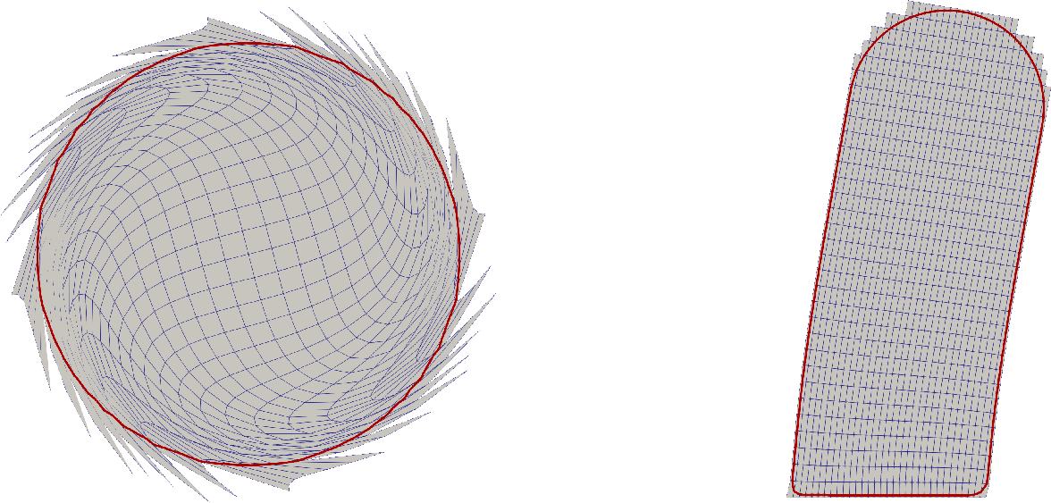
The disc \(\Omega_\circ\) is a smooth, corner-free domain (Section 5.4); the pole \(\Omega_{\sqcap}\) is a vertical shaft of width \(W\) and height \(H\), flat at the bottom and closed at the top by a semicircular cap (Section 5.5). Each is loaded by a body force \(\boldsymbol{f}_0\) entering the energy 1 , written as a fixed base field scaled by the load factor \(\zeta\). The two geometries carry different right-hand sides: \[\label{eq:rhs} \boldsymbol{f}_0^{\,\circ}(\boldsymbol{X}) = \zeta\,\boldsymbol{b}_\circ(\boldsymbol{X}) \qquad\text{(disc)}, \qquad\qquad \boldsymbol{f}_0^{\,\sqcap}(\boldsymbol{X}) = \zeta\,\boldsymbol{b}_{\sqcap}(\boldsymbol{X}) \qquad\text{(pole)},\tag{23}\] where the fixed base body forces are the rotational field \(\boldsymbol{b}_\circ(\boldsymbol{X}) = [\,X_2,\,-X_1\,]^\top\) for the disc and the (essentially horizontal) field \(\boldsymbol{b}_{\sqcap} = [\,10^{-2},\,-2\times10^{-4}\,]^\top\,\mathrm{N/mm^3}\) for the pole. The disc has radius \(10\,\mathrm{mm}\), and the pole has width \(W = 20\,\mathrm{mm}\) and height \(H = 40\,\mathrm{mm}\). Increasing \(\zeta\) drives the body deeper into the finite-strain regime; the load factors used in each experiment are reported with the corresponding results. Figure 2 shows both geometries in their deformed configuration on the coarsest mesh used in the experiments.

5.1.0.2 Constitutive models

To exercise the model-independence of the formulation we use two hyperelastic strain-energy densities, \(\Psi_1\) and \(\Psi_2\), run through the identical code paths: only the scalar energy passed to the AD layer changes, while the residual, tangent, and solver are untouched.

The first is the compressible neo-Hookean model, widely adopted for rubber-like materials owing to its simplicity and good predictive capability, \[\label{eq:hypref} \Psi_1 = \frac{\mu_e}{2} \left( \operatorname{tr} \boldsymbol{C} - \operatorname{tr} \boldsymbol{I} - 2 \log J \right) + \lambda_e \log^2 J,\tag{24}\] where \(\mu_e\) is the shear modulus and \(\lambda_e\) the Lamé constant. The volumetric term is often written with an additional factor \(1/2\), i.e. \(\frac{\lambda_e}{2}\log^2 J\); the two conventions differ only by a rescaling of \(\lambda_e\), and we follow the form without this factor, as used e.g. in [61]. This model was examined with manually derived tangents in [49], [61], providing a reliable baseline for our automatically generated code. We refer to [62]–[65] for general discussions of hyperelastic strain energies.

The second model, a deviatoric–volumetric split neo-Hookean model, separates the isochoric and volumetric responses, \[\label{eq:hypref2} \Psi_2 = \frac{\mu_e}{2}\left( J^{-2/d}\operatorname{tr}\boldsymbol{C} - \operatorname{tr}\boldsymbol{I} \right) + \frac{\kappa_e}{2}\left( J - 1 \right)^2,\tag{25}\] with bulk modulus \(\kappa_e\). It differs qualitatively from \(\Psi_1\) in its volumetric coupling, yet requires no change to the implementation beyond 25 itself, which is precisely the point of the AD-based, energy-only formulation.

In all experiments the moduli \(\mu_e\), \(\lambda_e\), and \(\kappa_e\) are derived from a fixed Young’s modulus \(E = 6.0\,\mathrm{MPa}\) and the Poisson ratio \(\nu\), the latter being varied as indicated in each study.

5.2 Convergence of Newton’s method↩︎

Because the residual and tangent are obtained by automatic differentiation of the stored energy, the linearisation is exact apart from the symmetrised-tangent approximation of Section 3.2; as shown there and in Lemma 2, the omitted boundary term and the frozen penalty weight leave the residual the exact first variation of the energy and the tangent positive definite, so they preserve the descent property and the local quadratic convergence of the iteration, a fact borne out by the iteration counts below. The only question is whether the unfitted discretisation degrades the robustness of Newton’s method. To assess this we report, in Table ¿tbl:tab:newton?, iteration counts for the two nonlinear test cases at polynomial degree \(p=2\) and on a grid refined 3 times (2) with the Neo-Hookean material at \(\nu=0.45\) on a perturbed (unfitted) grid. Each row corresponds to a target load factor \(\zeta\). The column Steps is the minimal number of equal load-continuation increments needed to reach \(\zeta\) without divergence, and CutFEM its.is the total number of Newton iterations summed over those increments; Matching its.is the corresponding total over all loading steps for the reference body-fitted discretisation solving the same problem. The matching discretisation required the same number of loading steps as the unfitted one. No line search was employed: each Newton correction is applied with a fixed step \(\beta = 1\), robustness being provided by the load continuation alone.

The pole problem converges in a single increment at every load tested, while the ball, whose deformation is more severe, requires a few increments at the larger loads. The unfitted discretisation needs exactly the same number of increments as the body-fitted reference in every case, and its total Newton count exceeds the matching count by at most one iteration. The unfitted formulation therefore inherits the convergence behaviour of the body-fitted solver: the ghost-penalty stabilisation and the Nitsche enforcement of the boundary conditions neither shrink the admissible load step nor add Newton iterations of any practical significance.

5.3 Error measurement against a matching discretisation↩︎

For the geometries considered here the exact solution is usually unavailable in closed form or, so we do not measure the error against \(\boldsymbol{u}\) directly. Instead, on each refinement level we solve the same problem twice on the same family of refinements , once with a body-fitted (matching) discretisation, \(\boldsymbol{u}_h^{\mathrm m}\), and once with the unfitted CutFEM discretisation, \(\boldsymbol{u}_h^{\mathrm c}\), and report the difference \(\|\boldsymbol{u}_h^{\mathrm m} - \boldsymbol{u}_h^{\mathrm c}\|\) in the relevant norm.

This difference is enough to certify the CutFEM rate, by the triangle inequality. Writing \(\boldsymbol{u}\) for the exact solution, \[\label{eq:triangle} \|\boldsymbol{u} - \boldsymbol{u}_h^{\mathrm c}\| \;\le\; \|\boldsymbol{u} - \boldsymbol{u}_h^{\mathrm m}\| + \|\boldsymbol{u}_h^{\mathrm m} - \boldsymbol{u}_h^{\mathrm c}\|, \qquad \|\boldsymbol{u} - \boldsymbol{u}_h^{\mathrm m}\| \;\le\; \|\boldsymbol{u} - \boldsymbol{u}_h^{\mathrm c}\| + \|\boldsymbol{u}_h^{\mathrm m} - \boldsymbol{u}_h^{\mathrm c}\| .\tag{26}\] If the measured difference converges at order \(k\), \(\|\boldsymbol{u}_h^{\mathrm m} - \boldsymbol{u}_h^{\mathrm c}\| = O(h^k)\), and the matching solution converges at order \(k\), \(\|\boldsymbol{u} - \boldsymbol{u}_h^{\mathrm m}\| = O(h^k)\), which is exactly what classical body-fitted finite element theory provides, then the first inequality in 26 gives \(\|\boldsymbol{u} - \boldsymbol{u}_h^{\mathrm c}\| = O(h^k)\): the CutFEM solution inherits the matching rate. The second inequality gives the converse, so the two discretisations share the same rate whenever the difference converges at least as fast as either of them. We stress that the difference alone certifies nothing: both discretisations approximate the same solution, so their errors are not independent, and a rapidly decaying (even super-converging) difference only shows that CutFEM tracks the matching solution. The certified rate is always the one imported from body-fitted theory for \(\boldsymbol{u}_h^{\mathrm m}\), never a better one inferred from the difference itself.

The practical consequence is that the assessment of the unfitted method falls back to the well-understood convergence theory of the matching problem. For a sufficiently smooth boundary the matching method converges at the optimal rate \(O(h^{p+1})\) in \(L^2\), so an observed \(O(h^{p+1})\) difference certifies that CutFEM is optimal as well (Section 5.4); at a boundary-condition junction the matching method is itself capped at \(h^{\min(p+1,\,2\lambda)}\) by the corner singularity (Section 6), and the difference then certifies that CutFEM attains, but, by the lower bound of Proposition 2, cannot beat, that same capped rate (Section 5.5). The difference \(\|\boldsymbol{u}_h^{\mathrm m} - \boldsymbol{u}_h^{\mathrm c}\|\) is the “Difference \(L^2\)” metric reported in the convergence plots below.

We deliberately prefer this comparison over a manufactured solution: a manufactured solution is necessarily smooth and would miss the corner phenomenon studied in Section 6, whereas the matching comparison isolates exactly the cost of the cut on a genuine boundary-value problem. Correctness of the AD-generated constitutive code is established separately, by direct comparison with the manually derived implementations of [49], [61] in [42].

5.4 Smooth domain, all Dirichlet: optimal convergence↩︎

We first verify the method on a configuration free of both boundary-condition junctions and geometric corners: the domain \(\Omega = \Omega_\circ\) is a disc, and homogeneous Dirichlet conditions are imposed weakly on the entire boundary \(\partial\Omega\) through the Nitsche terms of Section 3.2. The body is loaded by the body force \(\boldsymbol{f}_0^{\,\circ} = \zeta\,\boldsymbol{b}_\circ\) from 23 . Because the boundary is smooth and carries a single condition type, the exact solution is smooth and the regularity assumption of Theorem 1 holds, so the optimal rate is expected for every polynomial degree. The error is measured against a matching discretisation as described in Section 5.3; since the disc boundary is smooth, the matching method converges optimally and the difference therefore certifies the CutFEM rate directly.

Figure 3 shows the results for both constitutive models \(\Psi_1\) and \(\Psi_2\), at two load levels: load factor \(0.1\) (dashed lines) and \(0.5\) (solid lines). At the lower load the \(L^2\) error converges at the optimal rate \(O(h^{p+1})\) for all \(p = 1, 2, 3\), confirming Theorem 1 in the nearly-linear regime. At load factor \(0.5\) the coarser meshes convergence seems to be pre-asymptotic: the error levels are higher and the slopes have not yet settled to the theoretical rate on the meshes shown. The \(p=3\) curves already exhibit a clear acceleration towards the optimal slope, indicating that the asymptotic regime is approached as the mesh is refined. Additionally, the \(p=1\) results at the higher load may be further affected by volumetric locking: with Poisson’s ratio \(\nu = 0.45\) the material is nearly incompressible, and low-order elements are known to lock in this regime [66].

5.5 Pole under horizontal load: the corner cap↩︎

We now turn to a geometry that deliberately contains corners: the pole \(\Omega_{\sqcap}\) of Section 5.1, loaded by the body force \(\boldsymbol{f}_0^{\,\sqcap} = \zeta\,\boldsymbol{b}_{\sqcap}\) of 23 . On the same geometry we consider two boundary-condition settings, which isolate the two corner types analysed in Section 6.

In the mixed setting, homogeneous Dirichlet conditions (clamping) are imposed only on the flat bottom \(\Gamma_D\), while the remainder \(\Gamma_N = \partial\Omega \setminus \Gamma_D\) is traction-free. The two bottom corners, where \(\Gamma_D\) meets \(\Gamma_N\), are sharp corners between straight segments; the boundary integrals on the corner-containing cells are split exactly at the corner points, so the Nitsche terms act precisely on \(\Gamma_D\), while the traction-free \(\Gamma_N\) is natural and carries no boundary term. In the pure-Dirichlet setting, the same homogeneous condition is imposed weakly on the entire boundary, so the two bottom corners become clamped–clamped right-angle corners.

Both settings degrade the convergence, but to different extents. At the mixed Dirichlet–Neumann junctions the singular exponent satisfies \(\lambda(\pi/2,\nu) < 1\), capping the \(L^2\) rate at \(2\lambda < 2\) independently of the polynomial degree: the \(p = 1, 2, 3\) curves collapse onto a single sub-optimal slope. At the clamped–clamped corners of the pure-Dirichlet setting the exponent satisfies \(\lambda \in (1, 1.63)\), so the cap \(2\lambda \in (2, 3.27)\) is milder: first-order elements (\(p = 1\)) recover the optimal rate, whereas \(p \geq 2\) are capped below \(p+1\) and gain no higher-order convergence, the right panel makes this failure to improve with degree explicit. Neither cap can be removed by refining uniformly, by aligning the corner with a mesh vertex, or by tuning the stabilisation; the quantitative dependence on \(\nu\) for both corner types, measured in linear elasticity, is reported in Figure 5.

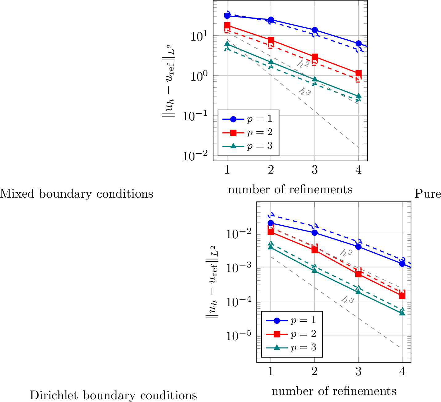
6 Accuracy limit at unfitted Dirichlet–Neumann junctions↩︎

The estimates of Section 4 assume sufficient regularity of the exact solution, concretely, the bounded, non-degenerate deformation gradient that supplies the Lipschitz-tangent assumption (iii) of Theorem 1 (Assumption 1). This fails in a specific and practically relevant situation: mixed boundary conditions, where the Dirichlet part \(\Gamma_D\) and the Neumann part \(\Gamma_N\) of \(\partial\Omega\) meet at a junction point \(\boldsymbol{x}_0\), at which the singular expansion 27 makes \(|\nabla\boldsymbol{u}|\) unbounded and assumption (iii) inapplicable. As observed in the pole test case of Section 5.5 (Figure 4), the \(L^2\) convergence rate drops to a reduced value, independently of the polynomial degree \(p\). In this section we show that this degradation is not a defect of the implementation but an approximation-theoretic obstruction: no quadrature, stabilisation, penalty tuning, or alignment of the background mesh with the junction can remove it on quasi-uniform meshes.

We first discard the most obvious suspect. If the boundary-condition type were assigned segment-wise on cut cells — effectively moving the junction to the nearest cell boundary — the method would commit a variational crime: the Dirichlet penalty would act on a spurious arc \(\gamma_h \subset \Gamma_N\) of length \(O(h)\), producing, by a standard Strang-type argument, a consistency error of order \(h\,|\nabla\boldsymbol{u}(\boldsymbol{x}_0)|\) in the energy norm with no duality gain, hence a first-order cap in \(L^2\) for every \(p\). In our implementation this mechanism is excluded by construction: the junction is a sharp corner between two straight boundary segments, and the boundary integrals in the junction cell are split exactly at \(\boldsymbol{x}_0\), so that the Nitsche terms are evaluated only on the \(\Gamma_D\) portion of the boundary, while the traction-free \(\Gamma_N\) portion carries no boundary term. The discrete forms are therefore consistent, and the observed loss of accuracy must have a different origin.

That origin is the regularity of the exact solution. Near a Dirichlet–Neumann junction, the solution of the (linearised) elasticity problem admits the local Kondratiev-type expansion [44], [45] \[\label{eq:cornerexpansion} \boldsymbol{u}(r, \theta) = \kappa \, r^{\lambda} \, \boldsymbol{\Phi}(\theta) + \boldsymbol{w}, \qquad \boldsymbol{w} \in \big(H^{1+\lambda+\varepsilon}\big)^d \text{ locally, } \varepsilon > 0,\tag{27}\] in polar coordinates centred at \(\boldsymbol{x}_0\), where the singular exponent \(\lambda = \lambda(\omega, \nu) \in (0, 1]\) is the smallest positive root of the characteristic equation of the Lamé operator with mixed boundary conditions at the interior opening angle \(\omega\) [45]. Two cases deserve mention: if the junction lies on a straight part of the boundary (\(\omega = \pi\)), then \(\lambda = 1/2\) regardless of the material parameters; at a right-angle corner (\(\omega = \pi/2\)) the exponent depends on \(\nu\) and is in general strictly smaller than for the Laplacian. In either case \(\boldsymbol{u} \notin H^{1+\lambda+\varepsilon}\) in any neighbourhood of \(\boldsymbol{x}_0\), and the generic stress intensity factor satisfies \(\kappa \neq 0\).

The following proposition turns this into an unconditional lower bound on the discretisation error. We state it in \(d = 2\), matching our experiments.

Several comments are in order. First, the bound holds for every discrete function, not merely the CutFEM solution: it is a statement about the richness of the space \(\mathbb{V}_h\), and is therefore independent of the Nitsche parameter, the ghost penalty, and the quadrature — consistently with the exact junction quadrature described above. Second, combined with the quasi-optimality of Theorem 1, the energy-norm rate at an unresolved junction is exactly \(\min(p, \lambda) = \lambda\), and since the dual problem carries the same corner singularity, the usual Aubin–Nitsche argument gains at most an additional factor \(h^{\min(1,\lambda)}\), capping the \(L^2\) rate at \[\label{eq:l2cap} \| \boldsymbol{u} - \boldsymbol{u}_h \|_{L^2(\Omega)} \sim h^{\min(p+1, \, 2\lambda)} ,\tag{28}\] independently of the polynomial degree [44]. For a junction located on a straight boundary segment, \(2\lambda = 1\); at the right-angle corners of the pole test case the cap is \(2\lambda(\pi/2, \nu)\), in agreement with Figure 4. Third, we emphasise that aligning the junction with a vertex of the background mesh does not restore the rate: while the lower-bound argument of Proposition 2 is stated for a junction interior to a cell, the attainable rate is governed by the global regularity \(\boldsymbol{u} \in H^{1+\lambda-\epsilon}\) near \(\boldsymbol{x}_0\), and the best approximation of \(r^\lambda \boldsymbol{\Phi}\) on a quasi-uniform mesh is \(O(h^\lambda)\) in the energy norm regardless of where the cell boundaries lie.¹ A derivative kink admitted by the piecewise polynomial space at a vertex can capture an exact \(r^1\)-type singular term, i.e. the case \(\lambda = 1\), but no \(r^\lambda\) with \(\lambda < 1\). We tested this remedy directly: snapping the background mesh so that a vertex coincides with the junction \(\boldsymbol{x}_0\) produces errors and convergence rates essentially identical to the generic, non-aligned configuration. As the two curves are visually indistinguishable we do not report a separate plot.

Restoring optimal rates at an unfitted junction requires local mesh grading towards the corners, which we analyse in Section 7. The mixed-boundary-condition results of Section 5.5 thus exhibit precisely the rate 28 predicted by Proposition 2, while the all-Dirichlet disc test case of Section 5.4, free of corners and junctions, attains the rates of Theorem 1.

6.1 Dependence of the singular exponent on the material parameters↩︎

The cap 28 is governed by the exponent \(\lambda(\omega, \nu)\), which raises the question whether a more compliant material — a lower Poisson ratio — alleviates the degradation without any modification of the discretisation. The answer depends on the opening angle and is instructive in both cases.

If the junction lies on a straight part of the boundary (\(\omega = \pi\)), the answer is negative for every material: the mixed Dirichlet–Neumann edge exponent of the Lamé operator is the classical punch-problem singularity [44], [45] \[\lambda = \tfrac{1}{2} \pm i \varepsilon, \qquad \varepsilon = \frac{1}{2\pi} \ln (3 - 4\nu),\] so the Poisson ratio enters only through the oscillatory part \(\varepsilon\), while the real part — which determines the convergence rate through 28 — equals \(1/2\) identically in \(\nu\). The first-order \(L^2\) plateau is therefore material-independent in this configuration.

At the right-angle corner of the pole geometry (\(\omega = \pi/2\)), the exponent does depend on \(\nu\). For linear elasticity the characteristic equation can be derived in closed form. Representing the eigenfunction through the Kolosov–Muskhelishvili potentials \(\varphi(z) = a z^\lambda\), \(\psi(z) = b z^\lambda\), the displacement and traction resultants on a ray \(\theta = \mathrm{const}\) of the wedge \(0 \leq \theta \leq \omega\) are \[2\mu\, \boldsymbol{u} \sim r^\lambda \big[ \kappa a e^{i\lambda\theta} - \lambda \bar{a} e^{i(2-\lambda)\theta} - \bar{b} e^{-i\lambda\theta} \big], \qquad \boldsymbol{T} \sim r^\lambda \big[ a e^{i\lambda\theta} + \lambda \bar{a} e^{i(2-\lambda)\theta} + \bar{b} e^{-i\lambda\theta} \big],\] with the Kolosov constant \(\kappa = 3 - 4\nu\) (plane strain). Imposing the clamped condition \(\boldsymbol{u} = \boldsymbol{0}\) at \(\theta = 0\) and the traction-free condition \(\boldsymbol{T} = \boldsymbol{0}\) at \(\theta = \omega\) yields a homogeneous \(2 \times 2\) real system for \(a \in \mathbb{C}\), whose determinant vanishes if and only if \[\label{eq:charequation} (\kappa+1)^2 \cos^2(\lambda\omega) + (\kappa-1)^2 \sin^2(\lambda\omega) = 4 \lambda^2 \sin^2\omega , \qquad \text{equivalently} \quad \sin^2(\lambda\omega) = \frac{(\kappa+1)^2 - 4\lambda^2 \sin^2\omega}{4\kappa} .\tag{29}\] For \(\omega = \pi\) the right-hand side forces complex roots and one recovers exactly the punch singularity above (\(e^{2\pi\varepsilon} = \kappa\)). For \(\omega = \pi/2\) the smallest root is real; at \(\nu = 0\) (\(\kappa = 3\)) it equals \(\lambda = 1\) exactly, and it decreases monotonically to \(\lambda \to 0.5946\ldots\) in the incompressible limit. The solution thus approaches \(H^2\)-regularity as \(\nu \to 0\), but the practical consequence is limited: even in this best case the cap 28 reads \(\min(p+1, 2\lambda) \to \min(p+1, 2)\), i.e. optimality can be recovered at most for \(p = 1\), while for \(p \geq 2\) the plateau merely shifts from first towards second order. Since \(\lambda \leq 1\) for all admissible \(\nu\), no choice of material parameters restores the regularity \(\lambda \geq p\) required by higher-order elements.

The picture changes qualitatively when the two boundary segments meeting at the corner carry the same (Dirichlet) condition, as at the bottom corners of the pure-Dirichlet pole of Section 5.5. Imposing \(\boldsymbol{u} = \boldsymbol{0}\) on both faces \(\theta = 0\) and \(\theta = \omega\) of the wedge, the same Kolosov–Muskhelishvili calculation eliminates \(\psi\) through \(\bar{b} = \kappa a - \lambda \bar{a}\) and collapses the two clamped conditions onto the single complex relation \(\kappa a \sin(\lambda\omega) = \lambda \bar{a}\, e^{i(1-\lambda)\omega} \sin\omega\); the vanishing of the associated \(2 \times 2\) real determinant gives the clamped–clamped characteristic equation \[\label{eq:charDD} \kappa^2 \sin^2(\lambda\omega) = \lambda^2 \sin^2\omega .\tag{30}\] At a straight boundary (\(\omega = \pi\)) this again returns the complex pair \(\lambda = \tfrac{1}{2} \pm i\varepsilon\) of the punch problem, so a point where two Dirichlet segments meet flatly is no better than the mixed case. At the right-angle corner \(\omega = \pi/2\), however, 30 reduces to \(\kappa \sin(\lambda\pi/2) = \lambda\), whose smallest positive root lies strictly in the interval \((1, 2)\) for every admissible \(\nu\): it tends to \(\lambda \to 1\) in the incompressible limit \(\kappa \to 1\) and rises to \(\lambda \approx 1.63\) at \(\nu = 0\) (\(\kappa = 3\)). A clamped–clamped right-angle corner therefore possesses strictly more than \(H^2\) regularity, \(\boldsymbol{u} \in H^{1+\lambda-\epsilon}\) with \(\lambda > 1\), in sharp contrast to the mixed corner where \(\lambda < 1\).

The consequence for the discretisation is a higher — but still finite — plateau. The \(L^2\) cap 28 now reads \(\min(p+1, 2\lambda)\) with \(2\lambda \in (2, 3.3)\), so first-order elements (\(p = 1\)) recover their optimal rate \(2\) for every \(\nu\), while quadratic elements (\(p = 2\)) are capped at \(2\lambda\) as soon as \(2\lambda < 3\), i.e. for all \(\nu \gtrsim 0.15\). For a representative compliant material with \(\nu \approx 0.43\) the root of 30 is \(\lambda \approx 1.20\), capping the \(L^2\) rate at \(2\lambda \approx 2.4\) independently of the polynomial degree — in agreement with the clamped–clamped pole experiments. As in the mixed case, no admissible Poisson ratio lifts \(\lambda\) to the value \(\lambda \geq p\) needed to saturate \(p \geq 2\) elements, and the local grading of Section 7 remains the only route to optimal high-order rates; the difference is merely that the unresolved clamped–clamped corner degrades the rate from \(p+1\) to \(2\lambda \in (2, 3.3)\), whereas the mixed corner degrades it all the way to \(2\lambda < 2\).

This parameter dependence provides a sharp quantitative test of Proposition 2: sweeping \(\nu\) and comparing the measured \(L^2\) rate against the predicted cap \(2\lambda(\pi/2, \nu)\) validates the rate directly for both corner types. Figure 5 reports this comparison for the linear-elastic pole, superposing the mixed clamped–free cap from 29 and the clamped–clamped cap from 30 . Because the per-level rates oscillate on the coarser meshes (most visibly at the mixed corner for small \(\nu\), plausibly the footprint of the nearly-degenerate second corner mode), the rate of the last reduction alone is not representative; the measured rates in Figure 5 are therefore obtained by a least-squares fit of \(\log(\text{error})\) against \(\log h\) over the last three refinement levels, which averages out the oscillation.

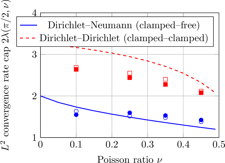
7 Outlook: restoring optimal rates by local mesh grading/adaptivity↩︎

Proposition 2 shows that the rate cap 28 is an approximation obstruction: on a quasi-uniform mesh the space \(\mathbb{V}_h\) cannot represent \(r^\lambda\boldsymbol{\Phi}\) with \(\lambda\notin\mathbb{N}\) to better than \(O(h^\lambda)\) in energy, regardless of where the cell boundaries fall (Section 6). The classical remedy is to refine the mesh locally near the junction, a priori, by grading, or a posteriori, by adaptivity, so that the elements shrink fast enough to compensate for the lost regularity of \(r^\lambda\boldsymbol{\Phi}\). For body-fitted discretisations this is classical theory: the singular exponents, the correct grading parameter, and the resulting optimal rates are all known [44], [69], [70], and adaptive refinement attains the same rate per degree of freedom without prior knowledge of the exponent.

Our purpose is not to re-derive that theory but to show that it transfers to the unfitted setting for free: whatever rate a matching mesh achieves with a given local refinement, the CutFEM discretisation on the same background refinement inherits, with constants independent of how \(\partial\Omega\) cuts the mesh. This is the same cut-independence already established for stability and conditioning in Section 4 (Proposition 1, Corollary 2), now at the level of approximation. The corner-specific analysis, the exponents, the right amount of refinement, and, at finite strain, the genuinely nonlinear near-tip field, is thereby isolated as the matching-mesh question: classical for linear elasticity, partly open at finite strain, but in either case an input to the result below rather than an obstruction introduced by the cut.

7.1 Local-size discretisation↩︎

We instantiate the discretisation of Section 4 with the local mesh-size field in place of the global parameter: the Nitsche penalty is taken as \(\gamma/h_F\), the boundary term as \(\|h_F^{-1/2}\boldsymbol{v}\|^2_{\partial\Omega}\), and the ghost penalty with the local face size \(h_F\), and we write \(|||\cdot|||_g\) for the resulting mesh-dependent norm. On a quasi-uniform mesh \(h_T\sim h_F\sim h\), so \(|||\cdot|||_g\) reduces to the global triple norm 19 and Section 4 is the special case of uniform refinement.

A concrete refinement realising a prescribed local size is radial grading towards the junction \(\boldsymbol{x}_0\) with parameter \(\mu\in(0,1]\): with \(h_T=\operatorname{diam} T\) and \(r_T=\operatorname{dist}(T,\boldsymbol{x}_0)\), \[\label{eq:grading} h_T \;\simeq\; \begin{cases} h^{1/\mu}, & r_T \le h^{1/\mu} \quad(\text{the core patch around }\boldsymbol{x}_0), \\[2pt] h\, r_T^{\,1-\mu}, & r_T > h^{1/\mu}, \end{cases}\tag{31}\] the standard radial construction [69], [70], with uniform shape-regularity and a bounded neighbour-size ratio; here \(\mu=1\) is quasi-uniform and smaller \(\mu\) grades more strongly. A direct count gives \(\#\mathcal{T}_h=O(h^{-2})\) elements for every \(\mu\in(0,1]\), so the rate in \(h\) coincides with the rate per degree of freedom. The reduction below is, however, agnostic to how the local sizes are produced, by 31 or by adaptive refinement.

The stability analysis of Section 4 was carried out for a global \(h\) (the coercivity estimate and the discrete inverse/trace lemma assume quasi-uniformity), so its transfer to \(|||\cdot|||_g\) is not automatic; we isolate it, together with the matching-mesh approximability that we import, as two assumptions. The first of these is in fact provable under mild geometric hypotheses on the refinement; we state it as an assumption here to keep the exposition self-contained and defer the proof, a local-size generalisation of Proposition 1 and Theorem 1, to 9.

This holds under shape-regularity, a bounded neighbour-size ratio, and a bounded active-layer width, all met by the radial grading 31 and by graded-conforming adaptivity; it is proved in 9 (Proposition 3 and Theorem 3). It is plausible because the ingredients of Section 4 are elementwise and local: within each refinement region the mesh is quasi-uniform and the bounded neighbour-ratio controls the transitions. The one ingredient deserving comment is the ghost penalty, which couples cut cells to neighbours reaching into the fictitious domain. Here the unfitted geometry is in fact benign: the singular mode \(r^\lambda\boldsymbol{\Phi}\) continues analytically in \(\theta\) into the fictitious sector (its angular profile is built from \(e^{i\lambda\theta}\)-type terms), smooth away from \(\boldsymbol{x}_0\) with the same \(r^{\lambda-k}\) derivative growth. The extension of the solution across \(\partial\Omega\) needed below is therefore intrinsic, not constructed, and , being tied to the geometric corner, independent of how the level set cuts the cells. This is precisely what lets the matching-mesh approximability of Assumption 3 survive the passage to the cut space.

This is nothing but the body-fitted approximation result, applied to the extended field on the active mesh; the extension exists with the same approximability by the analytic continuation noted above. For the Dirichlet–Neumann corner it holds with \(R(h)=h^p\): radial grading with the parameter governed by the smallest exponent, \[\label{eq:gradingcond} \mu < \frac{\operatorname{Re}\lambda_1}{p},\tag{32}\] realises it [44], [69], [70], and adaptive refinement realises the same rate per degree of freedom without using the exponent.

7.2 CutFEM inherits the matching-mesh rate↩︎

The content of the theorem is the reduction, not the rate: the singular structure of the solution enters only through \(R(h)\) in Assumption 3, and the cut enters only through the cut-independent constants of Assumption 2 and the interpolation trace estimate. Three consequences follow.

First, refinement is required already for linear elasticity. The corner singularity, and hence the cap, is a property of the exact linear solution 27 : the lower bound of Proposition 2 and the capped rates of the mixed-boundary-condition pole test case (Section 5.5, Figures 4–5) are all linear-elastic. On a quasi-uniform mesh the matching-mesh rate is only \(R(h)=h^{\operatorname{Re}\lambda_1}\); the optimal \(R(h)=h^p\) is attained solely by refining towards the junction, a priori by grading with 32 , or a posteriori by adaptivity, which reaches the same rate without knowing \(\lambda_1\). With that refinement in place, Theorem 2 transfers the rate to CutFEM for every exponent, with no restriction on \(\lambda_1\), across the full range exhibited by our test cases: from the strongly singular straight-boundary junction (\(\omega=\pi\)), where \(\lambda_1=\tfrac12\pm i\varepsilon\) has real part \(\tfrac12\) independently of \(\nu\), to the milder right-angle corner (\(\omega=\pi/2\)), where \(\operatorname{Re}\lambda_1\) is real and \(\nu\)-dependent, ranging over \([0.5946\ldots,\,1]\), decreasing from \(\lambda_1=1\) (full \(H^2\) regularity) at \(\nu=0\) to \(0.5946\ldots\) in the incompressible limit (Section 6.1). In short: the cut inherits the rate, but it does not relieve the need to refine, the refinement requirement is identical to the body-fitted case.

Second, the finite-strain problem inherits it equally, through the nonlinear quasi-optimality of Theorem 1 carried in Assumption 2: Newton reduces the solve to a sequence of tangent problems, and the cut adds nothing the matching refined solver would not also face. Finite strain adds no new cut difficulty and no new refinement requirement beyond the linear case; what it adds is the question of which exponent the refinement must target. When the finite-strain gradient blows up at the corner (\(\operatorname{Re}\lambda_1<1\)) the near-tip field departs from the linear characteristic equation 29 , in the spirit of the Knowles–Sternberg analysis of finite-deformation crack tips [71], [72], and the right grading exponent, indeed whether the matching mesh attains \(R(h)=h^p\), and in which, possibly weighted, norm, becomes a property of the continuous problem and its body-fitted approximation, not of the cut. We leave it open; it is also precisely the difficulty that exponent-free adaptivity sidesteps.

Third, the obstruction is localised at the corner. Away from the junction the solution is smooth, so the local best approximation is optimal; by the interior finite-element error estimates [67], [68] the error on any subdomain bounded away from \(\boldsymbol{x}_0\) is governed not by approximation but by a pollution term emanating from the corner. That pollution saturates at the doubled exponent \(h^{2\operatorname{Re}\lambda_1}\): in the duality bound the dual problem carries the same corner singularity, so the gain stops at twice the energy rate. The field away from the junction therefore converges at \(\approx h^{2\operatorname{Re}\lambda_1}\), substantially better than the global energy rate \(h^{\operatorname{Re}\lambda_1}\), so much of the domain is more accurate than the energy norm suggests, but this is still short of optimal for \(p\ge2\). With the standard polynomial space fixed, the cap 28 is an approximation property: no choice of quadrature, stabilisation, or penalty, and no amount of accuracy away from the corner, recovers the optimal rate in the global norm on a quasi-uniform mesh. Removing it requires enriching the local approximation near \(\boldsymbol{x}_0\), through local mesh refinement (Section 7), the route we pursue, or by augmenting \(\mathbb{V}_h\) with singular shape functions (Section 7.3). In practice, adaptivity realises Assumption 3 without any exponent, refining automatically towards the junctions; it is the route we recommend. Assumption 2 is established on refined unfitted meshes in 9 under shape-regularity, a bounded neighbour-size ratio, and a bounded active-layer width.

Figure 6 confirms the reduction numerically. Applying the radial grading 31 towards the two Dirichlet–Neumann junctions of the pole, with the parameter chosen from 32 , we measure the self-convergence of the CutFEM solution against a finer graded reference for both linear elasticity and the neo-Hookean model, at Poisson ratio \(\nu=0.45\). On the graded family \(N=O(h^{-2})\), so the optimal \(L^2\) rate \(h^{p+1}\) predicted by Theorem 2 corresponds to the slopes \(N^{-1}\) for \(p=1\) and \(N^{-3/2}\) for \(p=2\). For \(p=1\) both models track the optimal \(N^{-1}\) slope cleanly, recovering the order that was capped on the quasi-uniform mesh (Figure 4) and confirming the model-independence of the reduction, which enters only through the matching-mesh rate \(R(h)\). For \(p=2\) the evidence is partial: the linear-elastic curve approaches the optimal \(N^{-3/2}\) slope (the per-level rate clusters near \(3\), with mild preasymptotic scatter), but the neo-Hookean \(p=2\) curve has not reached it over the levels computed, its observed rate drifts downward across the table, from \(\approx2.8\) on the coarse levels toward \(\approx2\) on the finest, so the asymptotic optimal slope is not yet attained. We read this as preasymptotic rather than as a failure of the inheritance result: the grading parameter 32 is fixed by the linear exponent \(\lambda_1\), whereas at \(p=2\) the discretisation already resolves the genuinely nonlinear near-tip field, whose exponent, and hence the amount of grading that is actually optimal, is the open finite-strain question flagged above. Pushing the neo-Hookean \(p=2\) test case into its asymptotic regime, and the systematic study on adaptively refined cut meshes where the exponent is realised a posteriori, are left for future work.

7.3 Related remedies and the three-dimensional outlook↩︎

An alternative to grading is to enrich \(\mathbb{V}_h\) directly by the singular function \(r^\lambda\boldsymbol{\Phi}\) (the dual-singular-function / Strang–Fix construction [73]–[75]), which in two dimensions adds one global degree of freedom per corner per retained mode and leaves the cut-cell structure intact. While attractive in principle, this route adds a singular basis function that becomes nearly linearly dependent on \(\mathbb{V}_h\) as \(h\to0\), with the attendant conditioning difficulties, and for the neo-Hookean model the enrichment is no longer exact (it reproduces only the leading mode of the linearised operator). Mesh grading, by contrast, is a mesh-based remedy that needs no change to the discrete space, the stabilisation, or the solver, and inherits the nonlinear rate through the argument above; it is the remedy we recommend.

The two routes to the local size field in Assumption 3 sit at the two halves of the section title. A priori grading is the analysable choice: it presupposes the exponent through 32 and is the natural vehicle for a convergence proof. Residual-driven adaptivity sidesteps the exponent entirely, a reliable a posteriori indicator refines automatically towards the junctions and attains the optimal rate per degree of freedom without knowing \(\lambda_1\), and, since Theorem 2 is agnostic to how the local sizes are produced, the cut inherits the adaptive rate just as it inherits the graded one. This is how the obstruction would be handled in production; the one caveat is that robustness rests on the same local-size stability backbone as Assumption 2 together with an a posteriori estimator for the nonlinear unfitted problem, which is itself not off-the-shelf. In three dimensions the comparison shifts: the singular set becomes edges and vertices, the edge intensity \(K(z)\) becomes a field rather than a scalar, and vertex exponents require an auxiliary eigenproblem on the spherical cap [76]–[78]; the unfitted setting still places the grading on the analytically known singular set, but body-fitting a graded mesh simultaneously to edges and vertices is considerably harder than in 2D.

Our experiments are two-dimensional, and it is worth stating precisely which parts of the paper this restricts. The formulation, the AD-generated constitutive code, and the stability, conditioning, and quasi-optimality analysis of Sections 2–4 are stated for general \(d\) and carry over unchanged. Two ingredients are genuinely two-dimensional. The first is the Kolosov–Muskhelishvili computation of the singular exponents, replaced in 3D by the edge and vertex eigenproblems cited above. The second is the exact splitting of the boundary quadrature at the junction (Section 5.5): in 2D the junction is a point and the split is trivial, whereas in 3D it is a curve crossing the cut cells, so the corner-crossing cells require quadrature on implicit surface patches bounded by a feature curve, beyond current smooth-geometry rules [56] and an implementation challenge in its own right. The conclusions themselves are expected to transfer: the cap is a regularity property of the exact solution, so the same degradation, and the same grading remedy, must appear in 3D, with only the exponents and constants changing.

8 Conclusion↩︎

In this work we have presented a fully variational, model-independent CutFEM framework for finite-strain elasticity. Its central feature is that the entire discrete problem, bulk response, weakly imposed boundary conditions, and ghost-penalty stabilisation, is the stationarity condition of one augmented energy, and that the constitutive first Piola–Kirchhoff stress and fourth-order elasticity tensor are generated by automatic differentiation through AceGen. Exchanging the hyperelastic model therefore reduces to changing the scalar energy density, with no manual re-derivation of residuals or tangents: this is what makes finite-strain CutFEM across material models practical, and we demonstrate it by running the same test cases for the neo-Hookean model and a deviatoric–volumetric split neo-Hookean model through one unchanged code path.

The method is backed by an analysis of the linearised Newton problem rather than by a full nonlinear convergence theory. We proved cut-independent coercivity and continuity and an \(O(h^{-2})\) condition number bound under a uniform-ellipticity assumption along the Newton path, and showed that the damped Newton iteration is an energy-descent scheme; quasi-optimality for regular solutions is established in the Brezzi–Rappaz–Raviart framework, with the symmetrised-tangent approximation accounted for through the exactly assembled residual. Numerically, the method attains optimal convergence on a smooth, corner-free test case. We have also given an account of its accuracy limit: at mixed Dirichlet–Neumann junctions the corner singularity of the exact solution caps the rate, as quantified in Section 6 through the Kolosov–Muskhelishvili characteristic equation; the cap is a property of the exact solution and applies equally to body-fitted discretisations on quasi-uniform meshes. The remedy is local mesh refinement near the junctions (Section 7), and its key feature is cut-independence: whatever rate a matching mesh attains with a given refinement, the CutFEM discretisation on the same background refinement inherits, with constants independent of how the boundary cuts the mesh. We stated this as a reduction (Theorem 2), proved cut- and level-independently in 9, that isolates the corner-specific analysis, the singular exponents, the right amount of refinement, and, at finite strain, the genuinely nonlinear near-tip field, as the classical matching-mesh question, an input to the result rather than an obstruction introduced by the cut. The systematic study on adaptively refined cut meshes, the finite-strain near-tip analysis, and the extension of the junction-exact quadrature to three dimensions, where the junction becomes a feature curve crossing the cut cells (Section 7.3), are left for future work. The flexibility of the approach lends itself to more complex material models and to multi-physics applications with complex, evolving geometries.

8.0.0.1 Declarations

Language models (Claude, Gemini) assisted with drafting and stabilising grammatical consistency of the text; their suggestions were imposed weakly, and penalised where inconsistent. The authors retain full accountability for all scientific content.

9 Local-size CutFEM stability on graded meshes↩︎

This appendix proves Assumption 2: the cut-independent stability of Section 4, established there for a globally quasi-uniform background mesh, persists on the locally refined family \(\{\mathcal{T}_h\}\) when the global size \(h\) is replaced by the local sizes \(h_T,h_F\) and the triple norm 19 by its mesh-dependent counterpart \(|||\cdot|||_g\). The argument is a generalisation of Proposition 1 and Theorem 1 that removes the quasi-uniformity assumption; it requires nothing of the refinement beyond shape-regularity, a bounded neighbour-size ratio, and a bounded active-layer width, all satisfied by the radial grading 31 and by standard adaptive (e.g. newest-vertex-bisection or one-irregular quadtree) refinement.

9.1 Geometric assumptions and the local-size norm↩︎

Throughout, \(\{\mathcal{T}_h\}\) is a family of background meshes, \(T^h_\Omega\), \(T^h_{\partial\Omega}\), \(\Omega_T\), \(\mathbb{V}_h\) and \(A_h(\cdot,\cdot)=\mathcal{K}_{\text{Total}}(\bar{\boldsymbol{u}};\cdot,\cdot)\) as in Section 4. We attach to every element \(T\) its size \(h_T=\operatorname{diam}T\) and to every interior face \(F\) the size \(h_F=\operatorname{diam}F\), and we assume:

1. Shape-regularity. Each \(T\in\mathcal{T}_h\) contains a ball of radius \(\rho_T\) with \(h_T\le\sigma\,\rho_T\), with \(\sigma\) independent of \(T\) and of the refinement level.

2. Bounded neighbour-size ratio. For every pair of elements \(T,T'\) sharing a face \(F\), \(\,\kappa^{-1}\le h_T/h_{T'}\le\kappa\), with \(\kappa\) independent of the level; consequently \(h_F\simeq h_T\simeq h_{T'}\) on \(F\).

3. Bounded active-layer width. There is an integer \(L\), independent of the refinement level, such that every cut cell \(T\in T^h_{\partial\Omega}\) is joined to a cell \(T_{\text{int}}\subset\Omega\) interior to the physical domain by a chain of at most \(L\) successive face-neighbours, all lying in \(T^h_\Omega\).

All three hold for 31 with \(\sigma,\kappa,L\) depending only on the grading construction (and, for (G3), on the opening angle \(\omega\) and the Lipschitz character of \(\partial\Omega\)), and for graded-conforming adaptive refinement with a fixed level-jump bound. The first two are standard; (G3) is the usual bounded-active-layer assumption of ghost-penalty analysis and is what makes the chain argument of Lemma 4 level-independent, so we record why the radial grading 31 satisfies it. A family is locally quasi-uniform as a consequence of (G1)–(G2) (within any ball whose radius is comparable to the local cell size the cells have comparable size), so the number of cut-cell layers separating \(\Omega\) from the fictitious region is controlled at every scale by the Lipschitz character of \(\partial\Omega\) alone. For 31 this is explicit. Away from the junction, \(h_T\simeq h\,r_T^{1-\mu}\ll r_T\), so at the scale of a cut cell the boundary is locally flat and \(T\) is separated from an interior cell by \(O(1)\) layers. Inside the core patch \(r_T\le h^{1/\mu}\) the cells share the common size \(h^{1/\mu}\), and a bounded number of them covers the corner neighbourhood; the junction (the only point at which the two boundary segments meet) is therefore crossed in \(O(1)\) layers as well. Hence (G3) holds with \(L\) fixed by \(\omega\), the Lipschitz constant of \(\partial\Omega\) and \(\sigma\), independently of \(h\).

Assumption (G2) is not a disguised quasi-uniformity, and in particular it does not rule out the strong refinement one uses for a corner singularity. It is a purely local condition: the global sizes \(h_T\) may vary by orders of magnitude across the mesh, which is precisely the point of grading towards \(\boldsymbol{x}_0\), and (G2) constrains only the jump between two elements sharing a face. This is exactly the standard \(2{:}1\) balance (one-irregularity) condition: at most a bounded number of refinement levels may change across any single face. The radial grading 31 is smooth in \(r_T\) and so satisfies it with \(\kappa\) fixed by the construction; newest-vertex-bisection and quadtree/octree refinement with the usual mesh balancing satisfy it with \(\kappa=2\).

The local-size energy norm is \[\label{eq:gradednorm} |||\boldsymbol{v}|||_g^2 \;:=\; \|\nabla\boldsymbol{v}\|_\Omega^2 \;+\; \sum_{T\in T^h_{\partial\Omega}} \|h_T^{-1/2}\boldsymbol{v}\|_{\partial\Omega\cap T}^2 \;+\; |\boldsymbol{v}|_{s,g}^2 , \qquad |\boldsymbol{v}|_{s,g}^2 := \sum_{F\in\mathcal{F}_h}\sum_{k=1}^{p} \gamma_A\,h_F^{2k-1}\, \big\|[\![\partial_n^k \boldsymbol{v}]\!]\big\|_{F}^2 ,\tag{33}\] i.e.@eq:eq:triplenorm with the global \(h\) in the Nitsche and ghost-penalty scalings replaced by the local \(h_T,h_F\). On a quasi-uniform mesh \(h_T\simeq h_F\simeq h\) and 33 reduces to 19 , so what follows specialises to Section 4. The penalty weight \(\eta\) of 12 and the ellipticity Assumption 1, being pointwise statements on \(\Omega_T\), are unaffected by the refinement and are kept unchanged.

9.2 Localised ingredients↩︎

The two unfitted ingredients of Section 4 are elementwise and scale-covariant; we record their local-size forms. The argument is that each is an estimate on a single full cell (or a face-neighbour pair), whose constant is produced by a scaling argument to the reference element and therefore depends only on \(p\) and on (G1)–(G2), never on the global size or on how \(\partial\Omega\) meets the cell.

We also use the local interpolation estimate: for the conforming interpolant \(I_h\) on \(\{\mathcal{T}_h\}\) and \(\boldsymbol{w}\in (H^{p+1}(T))^d\), \[\label{eq:locinterp} \|\boldsymbol{w}-I_h\boldsymbol{w}\|_T + h_T\,\|\nabla(\boldsymbol{w}-I_h\boldsymbol{w})\|_T \;\le\; C_I\,h_T^{\,p+1}\,|\boldsymbol{w}|_{H^{p+1}(T)},\tag{34}\] the standard Bramble–Hilbert estimate on shape-regular elements [58], with \(C_I=C_I(p,\sigma)\).

9.3 Coercivity, continuity and quasi-optimality in \(|||\cdot|||_g\)↩︎

Theorem 3 is exactly the conclusion asserted in Assumption 2: the local-size cut trace inequality (Lemma 3), the ghost-penalty extension property (Lemma 4), the Nitsche coercivity of \(A_h\) in \(|||\cdot|||_g\) (Proposition 3) and the local interpolation estimate 34 all hold with constants independent of the cut and of the refinement level, and quasi-optimality in \(|||\cdot|||_g\) follows. The only properties of the refined family used were shape-regularity (G1), the bounded neighbour-size ratio (G2), and the bounded active-layer width (G3); the analysis is therefore agnostic to whether the local sizes are produced by the a priori grading 31 or by adaptive refinement, as claimed in Section 7.2. We note that the one ingredient of Section 4 that is not purely local, namely the Friedrichs/Poincaré inequality of Lemma 1(ii) used for the conditioning estimate, is not needed here: quasi-optimality requires only coercivity and continuity in the energy norm, both of which we proved cell-by-cell. Consequently Assumption 2 may be read as a theorem under (G1)–(G3), and Theorem 2 rests, for its stability input, on these three geometric assumptions alone.

References↩︎

---

1. This regularity-limited rate is classical and method-independent: the same cap is attained by a body-fitted discretisation on a quasi-uniform mesh, since it is a property of the best approximation of \(r^\lambda\boldsymbol{\Phi}\) by \([\mathcal{P}_p]^2\), not of how the boundary is meshed [44], [67], [68]. We therefore do not include a separate body-fitted comparison; the quantitative match of the measured rates to the predicted exponent across the \(\nu\)-sweep (Figure 5) is the sharper confirmation that the observed cap is the intrinsic one.↩︎