One More Time: Revisiting Neural Quantum States from a Reinforcement Learning Perspective
July 02, 2026
Abstract
Neural quantum states (NQS) provide a flexible and scalable framework for approximating quantum many-body wavefunctions. Among NQS parameterizations, autoregressive models are especially attractive because they enable exact, independent sampling from the Born distribution, avoiding the autocorrelation and mixing issues of Markov chain methods. Yet their optimization remains comparatively underexplored: Adam is a scalable method but ignores function space geometry, while stochastic reconfiguration is principled but costly and numerically fragile in large models. To address this gap, we show that variational energy minimization can be viewed as an advantage policy-gradient problem over the Born distribution, motivating trust-region optimization for NQS training. We introduce Proximal Wavefunction Optimization (PWO), a principled trust-region algorithm that clips probability-ratio changes in the amplitude channel and phase increments in the phase channel. PWO avoids explicit matrix inversion, reuses samples across multiple updates, and combines the scalability of first-order optimization with theoretical guarantees. Across Ising and frustrated \(J_1\)–\(J_2\) one- and two-dimensional spin systems, PWO improves stability and wall-clock convergence over Adam, minSR, and SPRING. Finally, we fine-tune a \(1.5\)B-parameter RWKV-7 model, demonstrating NQS optimization at a scale over three orders of magnitude beyond prior work.
0.0.1 Introduction↩︎
Quantum physics seeks to predict and understand the behavior of many interacting quantum particles. However, determining the exact ground (lowest-energy) state of a system of \(N\) quantum bits generally requires diagonalizing a \(2^N \times 2^N\) Hamiltonian matrix, quickly rendering exact methods intractable at scale. Variational approaches address this exponential complexity by optimizing a parameterized wavefunction ansatz to approximate the ground state. Neural quantum states (NQS) [1], [2] build upon this by using neural networks as expressive wavefunction representations, capable of capturing complex correlations [3] and high entanglement [4], as well as scaling to high-dimensional systems [5], where traditional methods struggle.
The practical success of NQS depends not only on expressivity but also on the ability to sample from and optimize the variational distribution. State-of-the-art NQS methods [6] primarily rely on Markov Chain Monte Carlo (MCMC) to estimate energies and gradients, which can introduce autocorrelation, slow mixing, and unreliable exploration in difficult regimes [7], [8]. Autoregressive NQS remove this sampling bottleneck by factorizing the Born distribution and enabling exact, independent sampling [9]–[11]. As a result, they provide a clean setting for variational optimization: samples can be drawn directly from the current wavefunction, and training dynamics are no longer confounded by Markov chain limitations. Despite these advantages, their adoption remains limited, as stable optimization is a central bottleneck for training accurate autoregressive models.
Existing optimization methods expose a sharp trade-off. First-order optimizers such as Adam [12] are computationally efficient and scale naturally to large neural networks, but they ignore the geometry of the variational wavefunction and can converge unstably or inaccurately in NQS applications [13], [14]. Stochastic reconfiguration (SR), and scalable variants such as minSR [15], are more geometrically principled because they approximate natural-gradient descent in wavefunction space. However, they require solving large and often ill-conditioned linear systems, with costs that become prohibitive for large networks or large sample regimes. Thus, autoregressive NQS resolve an important sampling problem, but stable first-order optimization of large autoregressive wavefunction models remains a central obstacle, which has been approached recently with transfer learning [16].
Contributions. This gap points to a missing optimization principle in NQS. In this work, we observe that the variational objective in NQS is mathematically equivalent to a policy-gradient objective in reinforcement learning (RL) under certain assumptions. While this connection has been implicitly present since early work [1], it has not been formalized or leveraged to design modern optimizers. In this work, we show that the RL-style trust-region optimization improves NQS training scalability and stability. Our contributions are as follows:
We formally connect variational energy minimization and policy-gradient RL, showing that the NQS gradient admits an advantage-weighted form over the Born distribution.
We introduce Proximal Wavefunction Optimization (PWO), an algorithm for NQS training inspired by Proximal Policy Optimization (PPO) [17], and prove that the PWO surrogate satisfies a trust-region improvement bound, allowing sample reuse.
We show that PWO improves the stability and convergence speed of autoregressive NQS compared to Adam and minSR on standard benchmarks (1D, 2D Ising and \(J_1\)–\(J_2\)).
Finally, we demonstrate the scalability of PWO by fine-tuning a 1.5 billion parameter RWKV-7 LLM [18] on the 1-D Ising model.
0.0.2 Background↩︎
0.0.2.1 Reinforcement Learning
Reinforcement Learning (RL) is a machine learning paradigm in which an agent learns to make decisions by interacting with an environment. At each time step \(t\), the agent observes a state \(s_t\), selects an action \(a_t\), and then receives a reward \(r_{t+1}\) and a new state \(s_{t+1}\) from the transition function \(P(\cdot| s_t, a_t)\). The goal of the agent is to learn a policy that maximizes the expected return over time. Let \(\pi_{\boldsymbol{\theta}}\) denote a policy parameterized by \(\boldsymbol{\theta}\). Formally, the return is defined over a trajectory \(\tau := (s_0, a_0, r_1, s_1, a_1, r_2, \dots)\), which is a sequence of states, actions, and rewards generated by the agent-environment interaction. Following the notation of [19], the probability of a trajectory \(\tau\) under \(\pi_{\boldsymbol{\theta}}\) is given by \[\mathcal{P}_{\boldsymbol{\theta}}(\tau) = \mu(s_0) \pi_{\boldsymbol{\theta}}(a_0 | s_0) P(s_1 | s_0, a_0)\pi_{\boldsymbol{\theta}}(a_1 | s_1) P(s_2 | s_1, a_1)\ldots,\]
where \(\mu(s_0)\) denotes the initial distribution over states. The objective of RL is to find a policy that maximizes the expected discounted return, which is captured by the state-value and action-value functions of a policy \(\pi_{\boldsymbol{\theta}}\): \[V^{\pi_{\boldsymbol{\theta}}}(s) := \mathbb{E}_{\pi_{\boldsymbol{\theta}}}\!\left[\sum_{t=0}^{\infty}\gamma^t r_{t}\,\middle|\, s_0=s\right], \quad Q^{\pi_{\boldsymbol{\theta}}}(s,a) := \mathbb{E}_{\pi_{\boldsymbol{\theta}}}\!\left[\sum_{t=0}^{\infty}\gamma^t r_{t}\,\middle|\, s_0=s,\;a_0=a\right],\] respectively. In policy optimization, an agent maximizes its expected return by performing gradient ascent with a policy gradient estimator [20] of the form: \[\label{eq:REINFORCE} \grad_{\boldsymbol{\theta}}V^{\pi_{\boldsymbol{\theta}}}(\mu) = \mathbb{E}_{\tau \sim \mathcal{P}_{\boldsymbol{\theta}}} \left[\sum_{t=0}^\infty \gamma^t A^{\pi_{\boldsymbol{\theta}}}(s_t, a_t) \grad_{\boldsymbol{\theta}} \log \pi_{\boldsymbol{\theta}} (a_t | s_t)\right].\tag{1}\] Here \(A^{\pi_{\boldsymbol{\theta}}}(s, a) := Q^{\pi_{\boldsymbol{\theta}}}(s, a) - V^{\pi_{\boldsymbol{\theta}}}(s)\) denotes the advantage of taking action \(a\) while in state \(s\), i.e., the expected return of taking action \(a\) relative to the policy average while in state \(s\).
0.0.2.2 Neural Quantum States
One of the key tasks in theoretical quantum many-body physics is to approximate the ground-state wavefunction of a system with many interacting particles. For a system of \(N\) spin-\(1/2\) particles, a configuration is a binary vector \(\vb{s}\in\{\pm 1\}^N\), and the wavefunction can be viewed as a complex vector \(\ket{\psi}\) in a Hilbert space \(\mathcal{H}\) (see Appendix 2.0.1) indexed by all \(2^N\) configurations. Equivalently, it defines a function \(\vb{s}\mapsto \psi(\vb{s})\), where \(\psi(\vb{s})\in\mathbb{C}\) is the amplitude assigned to configuration \(\vb{s}\): \[\ket{\psi} = \sum_{\vb{s}\in\{\pm1\}^N} \psi(\vb{s}) \ket{\vb{s}},\] where we use the Dirac, bra-ket, notation (see Appendix 2.0.1). The exponential size of this vector makes explicit representations intractable for large \(N\). Neural quantum states (NQS) address this by parameterizing the amplitude function with a neural network, \(f_{\boldsymbol{\theta}}\), so that \(f_{\boldsymbol{\theta}}(\vb{s})\) provides a compact approximation to \(\psi(\vb{s})\) [1], [21]. In practice, NQS models output the logarithm of the complex amplitude, \[f_{\boldsymbol{\theta}}(\vb{s}) = \log \psi_{\boldsymbol{\theta}}(\vb{s}) = \log \abs{\psi_{\boldsymbol{\theta}}(\vb{s})} + i\,\arg\psi_{\boldsymbol{\theta}}(\vb{s}) ,\] which separates the wavefunction into a log-modulus and a phase, usually handled by separate networks (channels). This representation is numerically convenient because amplitudes can vary over many orders of magnitude. By the Born rule, normalized wavefunctions induce a probability distribution over configurations, \(P_{\boldsymbol{\theta}}(\vb{s}) \propto \abs{\psi_{\boldsymbol{\theta}}(\vb{s})}^2\). In this work, we focus on autoregressive NQS, which explicitly factorize \(P_{\boldsymbol{\theta}}\) and enable exact independent sampling from the Born distribution.
0.0.2.3 Finding the Ground State
The Hamiltonian \(\hat{H}\) is the energy operator of a quantum system: it encodes the interactions, external fields, and kinetic terms that determine which wavefunctions have low or high energy. A popular application of the NQS framework is to find the ground state of quantum systems. Given a description of a physics system within a Hamiltonian, \(\hat{H}\), the ground state is the eigenstate \(\ket{\psi_0}\) corresponding to the lowest eigenvalue \(E_0\). This can be cast as a minimization problem: \[E_0\leq E[\psi] = \frac{\mel{\psi}{\hat{H}}{\psi}}{\braket{\psi}},\quad\forall\ket{\psi}\in\mathcal{H},\] where the equality holds if and only if \(\ket{\psi}\) belongs to the ground-state eigenspace – this is known as the variational principle. Taking this variational formulation of the ground state as the starting point, so-called variational methods define a parametric family of states \(\ket{\psi_{\boldsymbol{\theta}}}\) and approximate the ground state by solving \[\label{eq:vmc95objective} \boldsymbol{\theta}^* = \mathop{\mathrm{argmin}}_{\boldsymbol{\theta}} E[\psi_{\boldsymbol{\theta}}] = \mathop{\mathrm{argmin}}_{\boldsymbol{\theta}} \frac{\langle \psi_{\boldsymbol{\theta}} | \hat{H} | \psi_{\boldsymbol{\theta}} \rangle}{\langle \psi_{\boldsymbol{\theta}} | \psi_{\boldsymbol{\theta}} \rangle}.\tag{2}\] In the case of NQS, this family of functions is given by a neural network, as already discussed.
0.0.2.4 Variational Monte Carlo
To efficiently compute a minimizer of Eq. 2 , NQS uses Monte Carlo estimates. This approach is known as variational Monte Carlo (VMC). In particular, the energy can be written as \[E[\psi_{\boldsymbol{\theta}}] = \frac{\mel{\psi_{\boldsymbol{\theta}}}{\hat{H}}{\psi_{\boldsymbol{\theta}}}}{\braket{\psi_{\boldsymbol{\theta}}}{\psi_{\boldsymbol{\theta}}}} = \sum_{\vb{s}} \mathcal{P}_{\boldsymbol{\theta}}(\vb{s})\, E^{\mathrm{loc}}_{\boldsymbol{\theta}}(\vb{s}) = \mathbb{E}_{\vb{s}\sim \mathcal{P}_{\boldsymbol{\theta}}}\!\left[E^{\mathrm{loc}}_{\boldsymbol{\theta}}(\vb{s})\right], \label{eq:energy95expectation}\tag{3}\] where we define \[\mathcal{P}_{\boldsymbol{\theta}}(\vb{s})=\frac{\abs{\psi_{\boldsymbol{\theta}}(\vb{s})}^2}{\sum_{\vb{s}'}\abs{\psi_{\boldsymbol{\theta}}(\vb{s}')}^2}, \quad E^{\mathrm{loc}}_{\boldsymbol{\theta}}(\vb{s}) := \sum_{\vb{s}'}\frac{\psi_{\boldsymbol{\theta}}(\vb{s}')}{\psi_{\boldsymbol{\theta}}(\vb{s})}\mel{\vb{s}}{\hat{H}}{\vb{s}'}.\] With this formulation, NQS estimates the loss function by sampling a set of spin configurations \(\{\vb{s}_i\}_{i=1}^M\) from the parameterized distribution \(\mathcal{P}_{\boldsymbol{\theta}}\) and computing the sample mean of \(E^{\mathrm{loc}}_{\boldsymbol{\theta}}(\mathbf{s}_i)\): \[L(\boldsymbol{\theta}) \approx \bar{E}_{\boldsymbol{\theta}}^{\mathrm{loc}} \equiv \frac{1}{M} \sum_{i=1}^M E^{\mathrm{loc}}_{\boldsymbol{\theta}}(\mathbf{s}_i).\] By differentiating Eq. 3 (see Appendix 2.0.2.2) it is possible to show that its gradient with respect to \(\boldsymbol{\theta}\) can be expressed as an expected value over \(\mathcal{P}_{\boldsymbol{\theta}}\) and estimated using either MCMC sampling or direct sampling of autoregressive models: \[\label{eq:vmc} \partial_{\theta_i}L(\boldsymbol{\theta}) = \mathbb{E}_{\vb{s}\sim\mathcal{P}_{\boldsymbol{\theta}}}\bqty{2\Re\Bqty{ \pqty{E^{\mathrm{loc}}_{\boldsymbol{\theta}}(\mathbf{s}) - \mathbb{E}_{\mathbf{s}\sim\mathcal{P}_{\boldsymbol{\theta}}}[E^{\mathrm{loc}}_{\boldsymbol{\theta}}(\mathbf{s})]}O_i(\vb{s})^\ast }},\tag{4}\] for \(i=1,\ldots, P\), where \(O_i(\vb{s}) = \partial_{\theta_i}\log\psi_{\boldsymbol{\theta}}\) are the so-called score functions.
0.0.2.5 Stochastic Reconfiguration
Stochastic Gradient Descent (SGD) [22] is a simple and effective optimization method in many scenarios. However, in the context of VMC, it can suffer from slow convergence and instability due to the complex geometry of the parameter space. The key issue is that small changes in the parameters, \(\boldsymbol{\theta}\), do not necessarily correspond to small changes in the quantum state \(\ket{\psi_{\boldsymbol{\theta}}}\).
Stochastic reconfiguration (SR) [23], which generalizes natural gradient descent [24] to VMC, preconditions the gradient \(\grad_{\boldsymbol{\theta}}L(\boldsymbol{\theta})\) to ensure that the distance between \(\ket{\psi_{\boldsymbol{\theta}}}\) at one training iteration and the next is small. This distance is given by the infidelity between the two states and approximated to second order by the Fubini-Study metric, \[S_{i j}= \operatorname{Re}\left\{\operatorname{Cov}_{\mathbf{s}\sim \mathcal{P}_{\boldsymbol{\theta}}}\left[O_{i}^{*}(\mathbf{s}), O_{j}(\mathbf{s})\right]\right\},\qquad i, j = 1,\ldots, P,\] which encodes the local geometry of the Hilbert space at the current parameter configuration. In mathematical terms, SR modifies the update rule in the following way: \[\boldsymbol{\theta}\leftarrow \boldsymbol{\theta}-\eta \mathbf{S}^{-1} \grad_{\boldsymbol{\theta}} L(\boldsymbol{\theta}),\] where \(\eta\in\mathbb{R}\) is the learning rate. We discuss the high computational costs of SR and its more recent improvements in Appendix 2.0.3.1, motivating the use of first-order optimization methods.
0.0.3 Proximal Wavefunction Optimization↩︎
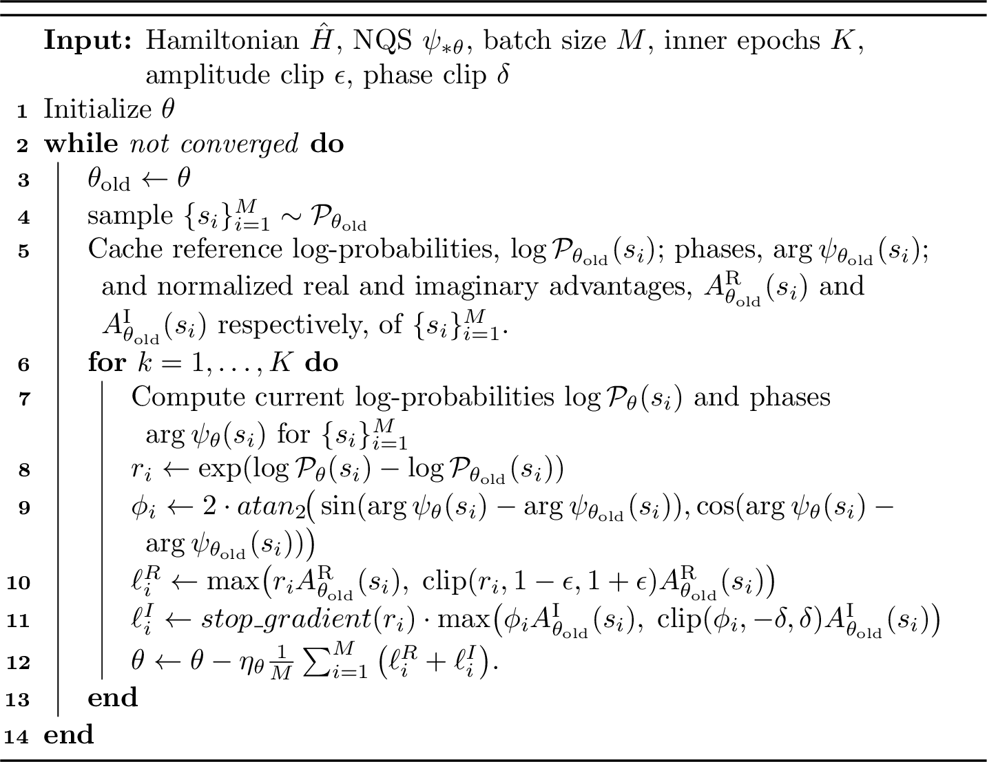
Here, we introduce a new optimization procedure for training NQS. We first draw an equivalence between the current NQS optimization paradigm and the policy gradient update in RL, and then use this to motivate applying Proximal Policy Optimization to
NQS.
propositionpgnqsprop
Assume the Hamiltonian is stoquastic, i.e. its matrix representation in a chosen computational basis has non-positive off-diagonal elements. Then we can assume \(f_{\boldsymbol{\theta}} = \log\psi_{\boldsymbol{\theta}} = \log\abs{\psi_{\boldsymbol{\theta}}}\), and the gradient of the variational energy can be written in policy-gradient form as \[\label{eq:pg95nqs} \grad_{\boldsymbol{\theta}} E[\psi_{\boldsymbol{\theta}}] = \mathbb{E}_{\vb{s}\sim\mathcal{P}_{\boldsymbol{\theta}}}\!\bqty{\pqty{E^{\mathrm{loc}}_{\boldsymbol{\theta}}(\mathbf{s}) - \mathbb{E}_{\mathbf{s}\sim\mathcal{P}_{\boldsymbol{\theta}}}[E^{\mathrm{loc}}_{\boldsymbol{\theta}}(\mathbf{s})]}\,\grad_{\boldsymbol{\theta}}\log \mathcal{P}_{\boldsymbol{\theta}}(\vb{s})}.\tag{5}\] In particular, variational energy minimization is equivalent to an advantage policy-gradient update over configurations. For a proof, see Appendix 2.0.2.1.
This proposition establishes a direct link between the NQS and RL frameworks (see also Tab. 1) by relating Eqs. 4 and 5 which motivates our algorithm, Proximal Wavefunction Optimization (PWO). The key observation is that the SR gradient is the result of solving the approximate constraint optimization problem of minimizing the expected energy while keeping the change in infidelity smaller than some quantity, \(\delta\). An analogous problem has been studied in the RL literature for a long time, but referred to as trust region optimization [17], [25], [26]. The fundamental idea is similar to that of SR: maximizing the expected reward while keeping the change in the total variation distance smaller than some quantity, \(\delta\).
Proximal Policy Optimization (PPO) [17], introduces a simple heuristic that empirically shows monotonic improvements by constraining updates to keep the updated policy close to the previous one. Applied to NQS, PPO would minimize the following surrogate loss: \[\label{eq:PPO} L_{\mathrm{mod}}^{\mathrm{clip}}(\boldsymbol{\theta}) = \mathbb{E}_{\vb{s} \sim \mathcal{P}_{{\boldsymbol{\theta}}_{\mathrm{old}}}} \left[ \max\left(r_{\boldsymbol{\theta}}(\vb{s}) A_{\boldsymbol{\theta}_{\mathrm{old}}}^{\mathrm{R}}(\vb{s}), \text{clip}(r_{\boldsymbol{\theta}}(\vb{s}), 1-\epsilon, 1+\epsilon)A_{\boldsymbol{\theta}_{\mathrm{old}}}^{\mathrm{R}}(\vb{s}) \right) \right],\tag{6}\] where \(r_{\boldsymbol{\theta}} = \mathcal{P}_{{\boldsymbol{\theta}}}/\mathcal{P}_{{\boldsymbol{\theta}}_{\mathrm{old}}}\) is the importance sampling ratio between the updated and previous distributions, \(\epsilon\) is the amplitude clip, the max comes from solving a minimization problem, and \[A_{\boldsymbol{\theta}_{\mathrm{old}}}^{\mathrm{R}}(\vb{s}) := \Re\Bqty{E^{\mathrm{loc}}_{\boldsymbol{\theta}_{\mathrm{old}}}(\vb{s})} - \mathbb{E}_{\vb{s}\sim \mathcal{P}_{\boldsymbol{\theta}_{\mathrm{old}}}} \left[\Re\Bqty{E^{\mathrm{loc}}_{\boldsymbol{\theta}_{\mathrm{old}}}(\vb{s})}\right],\] is the equivalent of the advantage estimate, yielding the local energy of configuration \(\vb{s}\) relative to the expected energy under the current NQS. In the case of RL, clipping ensures that policy updates remain conservative, thereby maintaining stability during optimization.
While PPO is a natural fit for the amplitude channel, it does not by itself account for the full VMC gradient. As shown in Appendix 2.0.2.3, the variational gradient also contains an imaginary component, which governs how the phase of the wavefunction should evolve. We, therefore, introduce a second proximal objective that controls phase updates directly by constraining the wrapped phase increment between the current and reference models. Concretely, letting \(\phi_{\boldsymbol{\theta}}(\vb{s})\) denote the wrapped phase difference (see Appendix 2.0.2.4), we minimize the clipped phase surrogate loss \[\label{eq:phase95clip} L_{\mathrm{arg}}^{\mathrm{clip}}(\boldsymbol{\theta}) = \mathbb{E}_{\vb{s}\sim \mathcal{P}_{\boldsymbol{\theta}_{\mathrm{old}}}} \left[ \operatorname{sg}\!\big(r_{\boldsymbol{\theta}}(\vb{s})\big)\, \max\!\left( \phi_{\boldsymbol{\theta}}(\vb{s})A_{\boldsymbol{\theta}_{\mathrm{old}}}^{\mathrm{I}}(\vb{s}), \mathrm{clip}\big(\phi_{\boldsymbol{\theta}}(\vb{s}),-\delta,\delta\big)A_{\boldsymbol{\theta}_{\mathrm{old}}}^{\mathrm{I}}(\vb{s}) \right) \right],\tag{7}\] where \(\operatorname{sg}(\cdot)\) denotes the stop-gradient operator (see Theorem 3), and \[A_{\boldsymbol{\theta}_{\mathrm{old}}}^{\mathrm{I}}(\vb{s}) := \Im\Bqty{E^{\mathrm{loc}}_{\boldsymbol{\theta}_{\mathrm{old}}}(\vb{s})} - \mathbb{E}_{\vb{s}\sim \mathcal{P}_{\boldsymbol{\theta}_{\mathrm{old}}}} \left[\Im\Bqty{E^{\mathrm{loc}}_{\boldsymbol{\theta}_{\mathrm{old}}}(\vb{s})}\right].\] The imaginary part of the local energy has zero expectation, so the centering is retained only to mirror the RL advantage. Equation 7 is the phase analog of PPO: instead of clipping a probability ratio, it clips the phase increment itself, preventing abrupt rotations of the wavefunction while still following the imaginary part of the VMC gradient. Using the phase increment instead of the ratio of phases ensures that the gradient of the combined loss (Eqs. 6 \(+\)7 ) matches the original one (Eq. 4 ) when we are on-policy, i.e., when the importance sampling ratio \(r_{\boldsymbol{\theta}}\) is one (no sample reuse).
| (l)3-4 Policy | \(\pi_{\boldsymbol{\theta}}(a\mid s)\) | Born distribution | \(\mathcal{P}_{\boldsymbol{\theta}}(\vb{s}) \propto |\psi_{\boldsymbol{\theta}}(\vb{s})|^2\) | |
| Advantage | \(A^{\pi_{\boldsymbol{\theta}}}(s_t,a_t)\) | Centered local energy | \(\Delta E(\vb{s}) = E^{\mathrm{loc}}_{\boldsymbol{\theta}}(\vb{s}) - E[\psi_{\boldsymbol{\theta}}]\) | |
| Policy gradient | \(A^{\pi_{\boldsymbol{\theta}}} \grad_{\boldsymbol{\theta}} \log \pi_{\boldsymbol{\theta}}\) | VMC force | \(2\Re\!\left[ \Delta E(\vb{s}) \grad_{\boldsymbol{\theta}} \log\psi_{\boldsymbol{\theta}}^\ast(\vb{s}) \right]\) | |
| KL trust region | \(D_{\mathrm{KL}} (\pi_{\boldsymbol{\theta}_{\mathrm{old}}} \| \pi_{\boldsymbol{\theta}})\) | Infidelity | \(\mathcal{I} (\psi_{\boldsymbol{\theta}}, \psi_{\boldsymbol{\theta}+\delta\boldsymbol{\theta}})\) | |
| Fisher matrix | \(\mathbf{F}\) | Fubini–Study metric | \(\mathbf{S}\) |
4pt
PWO combines the amplitude and phase losses into an efficient (see Appendix 2.0.3.2) first-order optimization procedure. For the amplitude channel, Proposition [prop:pg95nqs] shows that, when the phase is fixed, variational energy minimization takes the form of an advantage-weighted policy-gradient update over configurations, which naturally motivates a PPO-style clipped surrogate based on importance ratios. For the phase channel, Appendix 2.0.2.6 shows that the imaginary part of the VMC gradient can be conservatively optimized through a surrogate that constrains the phase increment. In practice, PWO performs \(K\) inner updates on a frozen batch of configurations sampled from the reference Born distribution \(\mathcal{P}_{\boldsymbol{\theta}_{\mathrm{old}}}\), clipping probability-ratio changes for the amplitude and wrapped phase increments for the phase. Because the same batch is reused across inner steps, the phase objective includes detached importance weights to correct for the mismatch between the reference and current sampling distributions (see Theorem 3). Algorithm 1 summarizes the resulting procedure.
0.0.4 Theoretical Analysis↩︎

The theoretical justification for PWO parallels monotonic-improvement analyses in policy optimization. In CPI [25] and TRPO [26], the true return change is controlled by a surrogate objective under a reference policy plus a penalty for moving too far from it. PWO follows the same principle with the return replaced by negative variational energy, probability ratios controlling the amplitude channel, and phase increments controlling the phase channel. Figure 2 illustrates this principle: trust regions make sample reuse possible by keeping optimization close enough to the reference wavefunction \(\psi_{\boldsymbol{\theta}_{\rm old}}\) so that the surrogate loss function evaluated on old samples remains a controlled approximation to the current energy landscape. Theorem [thm:pwo-gradient-consistency-main] shows that this proximal construction preserves the exact local VMC direction.
theoremfirstorderconsistency Let \(\ket{\psi_{\boldsymbol{\theta}}}\) be differentiable at \(\boldsymbol{\theta}_{\mathrm{old}}\), and assume common support. For \(\epsilon,\delta>0\), \[\left. \grad_{\boldsymbol{\theta}} \left( L^{\mathrm{clip}}_{\mathrm{mod}}(\boldsymbol{\theta}) + L^{\mathrm{clip}}_{\mathrm{arg}}(\boldsymbol{\theta}) \right) \right|_{\boldsymbol{\theta}=\boldsymbol{\theta}_{\mathrm{old}}} = \left. \grad_{\boldsymbol{\theta}}E[\psi_{\boldsymbol{\theta}}] \right|_{\boldsymbol{\theta}=\boldsymbol{\theta}_{\mathrm{old}}}.\] For a proof see Appendix [app::pwo-first-order-consistency-main-app].
Thus, the first PWO inner update exactly matches the VMC gradient; the surrogate only controls how far this direction is followed while reusing samples. For finite updates, local agreement is not enough. Let \(r_{\boldsymbol{\theta}}=\mathcal{P}_{\boldsymbol{\theta}}/\mathcal{P}_{\boldsymbol{\theta}_{\mathrm{old}}}\) and \(\alpha_{\boldsymbol{\theta}}\) be the wrapped phase increment and define \[\label{eq:pwo95linear95term} \mathcal{A}_{\boldsymbol{\theta}_{\mathrm{old}}}(\boldsymbol{\theta}) := 2\mathbb{E}_{\vb{s}\sim\mathcal{P}_{\boldsymbol{\theta}_{\mathrm{old}}}} \left[ \sqrt{r_{\boldsymbol{\theta}}} \left( \cos\alpha_{\boldsymbol{\theta}} A^{\mathrm R}_{\boldsymbol{\theta}_{\mathrm{old}}} + \sin\alpha_{\boldsymbol{\theta}} A^{\mathrm I}_{\boldsymbol{\theta}_{\mathrm{old}}} \right) \right],\tag{8}\]
theoreminfidelityimprovement Let \(\ket{\psi_{\boldsymbol{\theta}_{\mathrm{old}}}}\) and \(\ket{\psi_{\boldsymbol{\theta}}}\) be normalized wavefunctions with common support. Then \[\label{eq:pwo95infidelity95bound} E[\psi_{\boldsymbol{\theta}}]-E[\psi_{\boldsymbol{\theta}_{\mathrm{old}}}] \leq \mathcal{A}_{\boldsymbol{\theta}_{\mathrm{old}}}(\boldsymbol{\theta}) + 2\norm{\hat{H}-E[\psi_{\boldsymbol{\theta}_{\mathrm{old}}}]\mathbb{1}}_{\infty} \left( 1-\sqrt{1-\mathcal{I}( \psi_{\boldsymbol{\theta}_{\mathrm{old}}}, \psi_{\boldsymbol{\theta}} )} \right).\tag{9}\] For a proof see Appendix 2.0.2.4.
This bound is independent of clipping and holds for any finite update. The clipped PWO certificate follows by adding the stronger requirement that the realized update satisfies the amplitude and phase trust regions globally, not only on the sampled
batch (which is encouraged by the method but not guaranteed, see Appendix 2.0.2.7).
corollarypwoimprovement Assume the conditions of Theorem [thm:pwo-infidelity-improvement], bounded centered local energies, and global constraints \(r_{\boldsymbol{\theta}}(\vb{s})\in[1-\epsilon,1+\epsilon]\) and \(|\alpha_{\boldsymbol{\theta}}(\vb{s})|\leq\delta\) for all \(\vb{s}\), with \(0\leq\epsilon\leq1\) and \(0\leq\delta\leq\pi\). Then there exists \(C_{\boldsymbol{\theta}_{\mathrm{old}}}<\infty\) such that \[\label{eq:pwo95main95bound} E[\psi_{\boldsymbol{\theta}}]-E[\psi_{\boldsymbol{\theta}_{\mathrm{old}}}] \leq L^{\mathrm{clip}}_{\mathrm{mod}}(\boldsymbol{\theta}) + L^{\mathrm{clip}}_{\mathrm{arg}}(\boldsymbol{\theta}) + 2C_{\boldsymbol{\theta}_{\mathrm{old}}} \left( 1- \frac{1+\sqrt{1-\epsilon^2}}{2} \cos^2\!\left(\frac{\delta}{2}\right) \right).\tag{10}\] For a proof see Appendix 2.0.2.7.
The final term is the trust-region penalty. It vanishes as \(\epsilon,\delta\rightarrow0\) and grows as either clipping range is relaxed. Hence, if the clipped surrogate is minimized until the right-hand side of Eq. 10 is negative, the updated wavefunction is guaranteed to have lower energy. Together, the results show that PWO follows the exact local VMC direction, while finite-update errors are controlled generally by infidelity and, under global clipping, by explicit amplitude and phase trust-regions.
0.0.5 Experiments↩︎
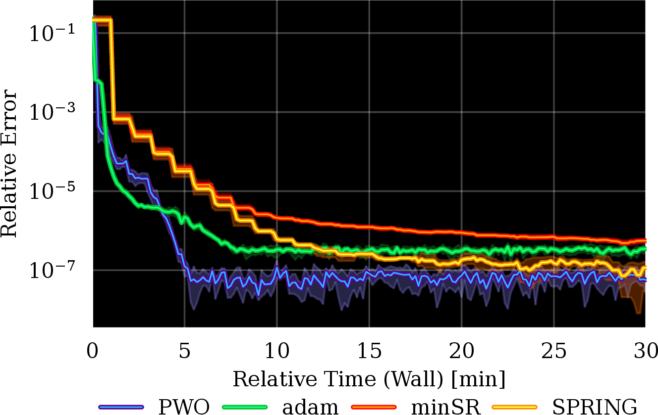

Figure 3: Comparison of PWO, Adam, minSR, and SPRING on the transverse-field Ising model over \(10\) random seeds. All methods were run with \(1024\) samples on a single NVIDIA L40S GPU..
0.0.5.1 Spin-chain benchmarks
We evaluate PWO for 1.5M-parameter autoregressive NQS on three different spin systems. Each systems consists of a one-dimensional spin-\(1/2\) chain of \(N=12\) sites with periodic boundary conditions, so that site indices are understood modulo \(N\). Let \(\hat{\sigma}_i^\alpha\), \(\alpha\in\{x,y,z\}\), denote the Pauli operator on site \(i\), and let \(\hat{\vb S}_i=1/2(\hat{\sigma}_i^x,\hat{\sigma}_i^y,\hat{\sigma}_i^z)\). For each Hamiltonian, we minimize the variational energy \(E[\psi_{\boldsymbol{\theta}}]\) and report the relative error with respect to the exact ground-state energy \(E_0\), \(\epsilon_{\rm rel} = (E[\psi_{\boldsymbol{\theta}}] - E_0) / E_0\), which can be computed for these relatively small systems. We also report the V-score [6], a scale-invariant convergence metric based on the energy variance that vanishes for exact eigenstates. The two Hamiltonians chosen offer increasing difficulty, as the underlying physics requires more complicated functions to represent. We use the same NQS architecture and the same number of Monte Carlo samples for all optimizers, so differences in performance reflect optimization rather than model capacity. For details about the hyperparameter search and the used architecture, see Appendices 2.0.4.1 and 2.0.4.2.
Transverse Field Ising Model. \[\hat{H}_{\mathrm{Ising}} = -J \sum_{i=1}^{N} \hat{\sigma}_i^z \hat{\sigma}_{i+1}^z -h \sum_{i=1}^{N} \hat{\sigma}_i^x. \label{eq:ising95hamiltonian}\tag{11}\] Here, \(J=1\) is the ferromagnetic coupling strength and \(h=1\) is the transverse-field strength. This Hamiltonian is a standard sign-problem-free benchmark: the diagonal interaction term favors aligned spin configurations, while the transverse field introduces quantum fluctuations by flipping individual spins. Therefore, Proposition [prop:pg95nqs] holds exactly.
Heisenberg \(J_1\)–\(J_2\) Chain. \[\hat{H}_{J_1\text{--}J_2} = J_1 \sum_{i=1}^{N} \hat{\vb S}_i \cdot \hat{\vb S}_{i+1} + J_2 \sum_{i=1}^{N} \hat{\vb S}_i \cdot \hat{\vb S}_{i+2}, \qquad J_1>0,\; J_2>0 . \label{eq:j1j295hamiltonian}\tag{12}\] We set \(J_1=1\) and \(J_2=0.5\), i.e., \(J_2/J_1=0.5\). At this ratio the next-nearest-neighbor interaction maximally frustrates the nearest-neighbor antiferromagnetic coupling, placing the system at the Majumdar–Ghosh point, where a highly entangled ground state with a complex sign structure makes both variational optimization and Monte Carlo sampling particularly challenging [23]. Unlike \(\hat{H}_{\mathrm{Ising}}\), the Hamiltonian \(\hat{H}_{J_1\text{--}J_2}\) requires a nontrivial sign structure in the computational basis; we use a complex-valued parameterization so that PWO can learn this structure through its phase channel. This setting evaluates whether the clipped phase surrogate (Eq. 7 ) remains a useful practical heuristic. We make an analogous study for \(J_1 = 0.25\) and \(J_2=0\) (the so-called Heisenberg chain) in Appendix 2.0.5.1.
All results are computed over \(10\) random seeds. Since several runs reach high-precision errors, numerical instabilities can produce extreme outliers. Mean-and-standard-deviation summaries are therefore poorly suited to this regime, as a single unstable run can distort both the central estimate and the uncertainty band. Following [27], we instead report interquartile statistics: at each evaluation time, curves show the interquartile mean (IQM), computed by averaging the middle \(50\%\) of seeds after discarding the lowest and highest quartiles. Shaded regions denote the interquartile range, from the \(25\)th to the \(75\)th percentile. This provides robust central estimates while still showing run-to-run variability. The figures with all individual seeds plotted are shown in Appendices 2.0.5.1-2.0.5.3. We discuss limitations of our approach in Appendix 2.0.3.4.
0.0.5.2 Convergence and Stability Results
Figure 3 shows that PWO converges the fastest of the four optimizers on the 1D Ising model, reaching relative error \(10^{-7}\) in approximately \(5\) minutes, while minSR requires approximately \(30\) minutes to reach the same accuracy. The V-score follows the same trend: PWO rapidly suppresses energy fluctuations, indicating that the proximal objective is not merely improving the energy estimate, but driving the state toward an eigenstate. Adam and SPRING also make steady progress, but require more wall-clock time to reach the same accuracy. minSR is stable on this easier Hamiltonian, but its per-step cost makes it substantially slower in wall-clock time.
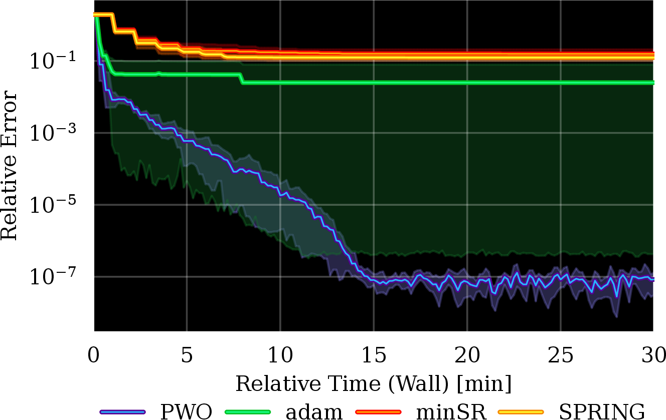
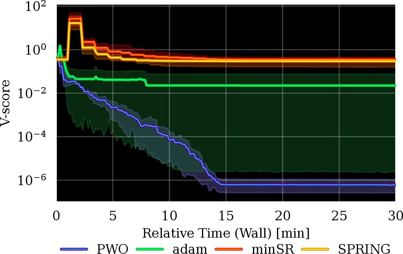
Figure 4: Comparison of PWO, Adam, minSR, and SPRING on the Heisenberg \(J_1\)–\(J_2\) chain over \(10\) random seeds. MinSR is highly unstable on this Hamiltonian, with \(6\) out of \(10\) runs producing NaNs. All methods were run with \(1024\) samples on a single NVIDIA L40S GPU..
On the \(J_1\)–\(J_2\) Hamiltonian in Figure 4, PWO reaches relative error \(10^{-7}\) in approximately \(15\) minutes while maintaining a steadily decreasing V-score, showing that the learned state is converging in both energy and variance. In contrast, Adam plateaus several orders of magnitude above PWO due to outliers. Also, the PWO contrast with minSR and SPRING is sharper than in the Ising case: minSR is numerically unstable, with \(6\) out of \(10\) runs producing NaNs, and both remain at a relative error of \(10^{-1}\) after \(30\) minutes. Despite using curvature-inspired updates, these methods struggle to make progress and exhibit numerical instability. This is the strongest empirical evidence for the central claim of the paper: a PPO-style proximal objective can retain the low wall-clock cost of first-order optimization while providing the stability needed to train expressive NQS on difficult quantum Hamiltonians. Experiments on the Heisenberg chain in Appendix 2.0.5.1 offer the same conclusion. We also plot all individual seed curves without aggregation or filtering for greater clarity and visibility in Appendix 2.0.5.1.
0.0.5.3 Two-dimensional \(J_1\)–\(J_2\) model on the square lattice
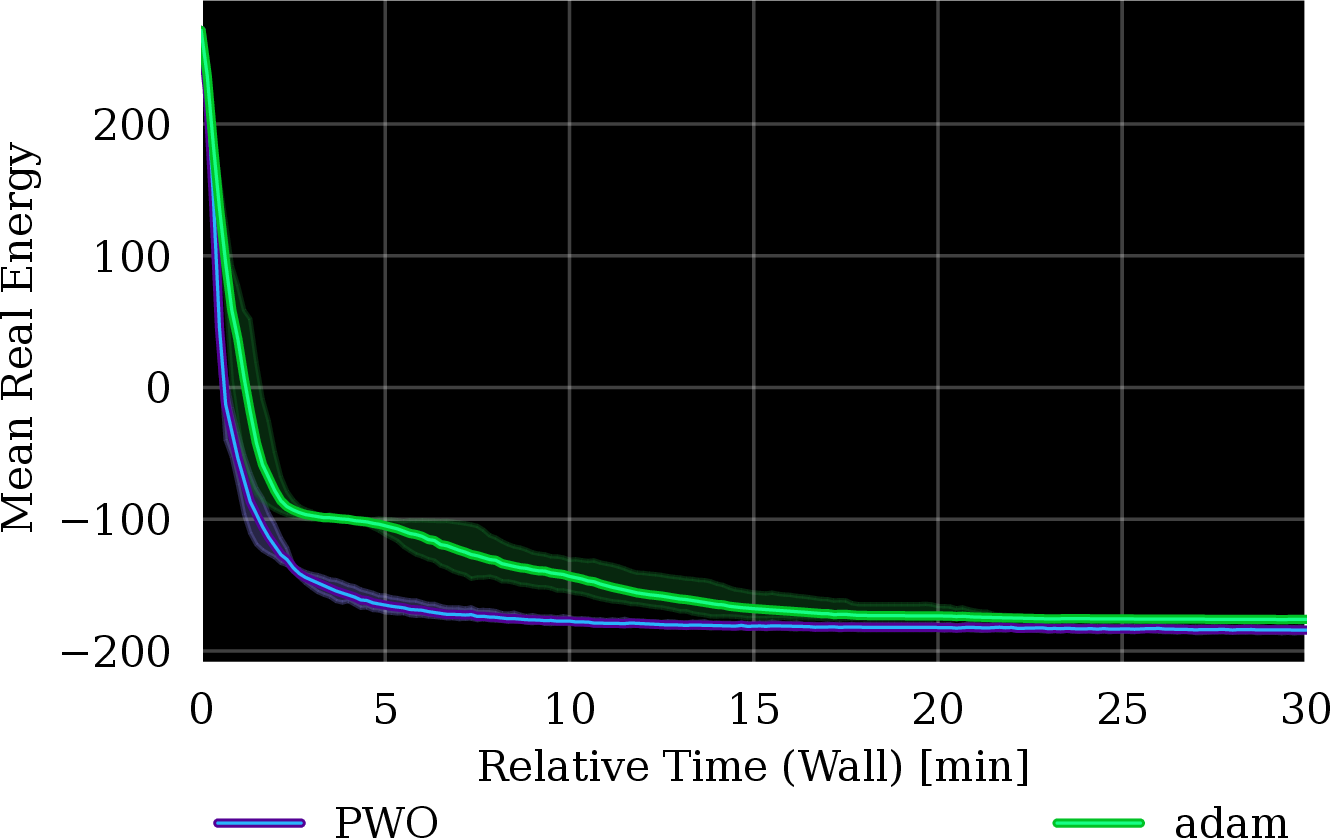

Figure 5: Two-dimensional frustrated \(J_1\)–\(J_2\) Heisenberg model on the \(10 \times 10\) lattice. Left: mean real energy. Right: V-score. PWO reaches lower energies faster than Adam and maintains a lower variance-based error signal over the same wall-clock budget..
We next test whether PWO remains effective beyond one-dimensional chains on a frustrated square-lattice \(J_1\)–\(J_2\) Heisenberg model with periodic boundary conditions and system size of \(10 \times 10\). We use a complex patch-autoregressive transformer with two-dimensional RoPE and enforce the zero-magnetization sector. Since exact diagonalization is intractable at this size, we compare optimizers using the mean real energy and the V-score. As shown in Fig. 5, PWO decreases the energy faster than Adam and reaches a lower-energy regime within the same wall-clock budget. The V-score follows the same trend, indicating that the proximal objective also improves stability on this frustrated two-dimensional benchmark. Individual seed runs are shown in Appendix 2.0.5.1.
0.0.5.4 Scalability Experiments
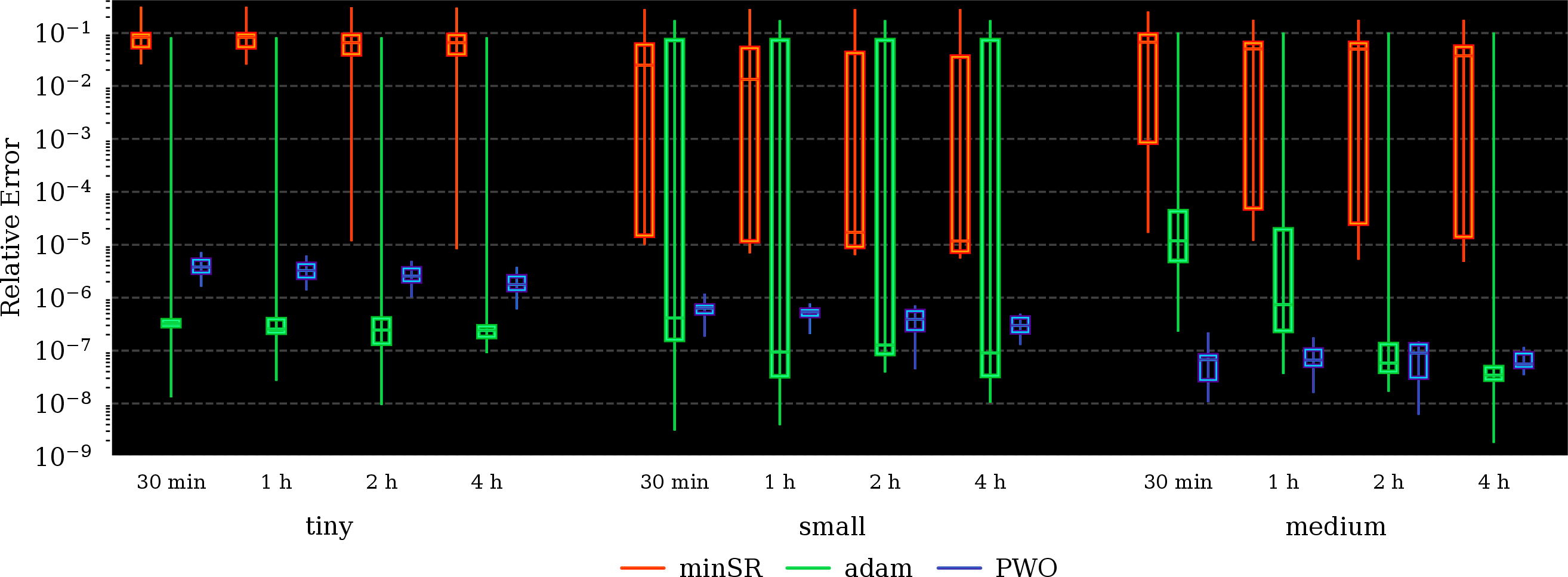
Figure 6 compares the scaling behavior of PWO, Adam, and minSR for increasing NQS model sizes on the Heisenberg \(J_1\)–\(J_2\) chain (see Appendix 2.0.4.7 for details). PWO exhibits consistent stability and monotonic energy improvement as NQS size grows, reaching near-final energies within the first 30 minutes. In contrast, minSR is both unstable and never reaches competitive energy values. Adam performs best for the tiny network, but degrades in stability and efficiency for small and medium NQS, where PWO is both faster and more reliable. In particular, achieving comparable energy scales with the medium NQS requires roughly \(4 \times\) more time with Adam than with PWO. In Appendix 2.0.3.2, we show that PWO converges faster than other optimizers because it does more optimization steps per unit of time. Although Adam attains lower energies after extended training of 4 hours, the observed scaling trend suggests that this advantage may diminish for yet larger networks. In Appendix 2.0.5.2 we perform additional scaling experiments on the number of samples and system size.
0.0.5.5 NQS Fine-tuning of Large Language Models


Figure 7: Fine-tuning curves of a 1.5B-parameter RWKV7LLM on the 1-D Ising Model..
Figure 7 shows fine-tuning results for a \(1.5\)B-parameter RWKV-7 model on the transverse-field Ising chain. PWO achieves a lower final relative error and V-score than Adam, while maintaining stable training across the full wall-clock budget. This improvement is not meant to establish that LLMs or large networks [28] are the right inductive bias for one-dimensional Hamiltonians; rather, it shows that the proximal objective is effective when the ansatz is scaled by more than three orders of magnitude beyond existing NQS in the literature [29].
0.0.6 Related Work↩︎
Reinforcement Learning and Ground State Search. Ground state search has been treated as an optimal control problem via Feynman-Kac representations [30], and RL frameworks have been developed for lattice models by treating stoquastic Hamiltonians as reward functions [31]. Recent meta-learning approaches [32] leverage RL to optimize the quantum state learning process itself. However, these works apply RL by either reformulating the problem theoretically or optimizing the learning procedure. We instead use RL as the primary optimization framework applying it directly on the NQS ansatz.
Importance Sampling and Trust Regions. Sample reuse and proximal objectives have been previously explored for non-autoregressive NQS optimization. [33] introduced importance sampling gradient optimization (ISGO), which reuses Markov chain samples across multiple gradient updates by reweighting local energies with the probability ratio between the current and reference wavefunctions. Building on this, [34] introduced a PPO-inspired a cosine penalty on phase variation. Our work formalizes the analogy with RL in Proposition [prop:pg95nqs], uses a different clipping objective directly on the imaginary gradient instead of a penalty, and makes the policy-gradient correspondence exact, allowing stable training of billion-parameter models for the first time.
0.0.7 Conclusion↩︎
We introduced Proximal Wavefunction Optimization (PWO), a scalable first-order optimizer for neural quantum states (NQS) derived from an explicit connection between variational Monte Carlo and reinforcement learning (RL). In the fixed-phase stoquastic setting, we showed that variational energy minimization can be written as an advantage policy-gradient objective over the Born distribution, where spin configurations play the role of actions and centered local energies act as advantages. This reformulates NQS optimization into a trust-region policy-optimization problem, motivating a PPO-style algorithm that clips probability-ratio changes in the amplitude channel and extends naturally to complex wavefunctions through a clipped phase-increment surrogate. Across spin-chain benchmarks, PWO improves wall-clock convergence and stability over Adam, minSR, and SPRING, with the largest gains in frustrated regimes where optimization is most fragile. Finally, by fine-tuning a \(1.5\)B-parameter RWKV-7 model as an autoregressive NQS, we bring NQS training into the regime of modern large-scale sequence modeling. More broadly, our results bridge the RL and NQS communities, enabling further mutual inspiration. By unlocking large autoregressive NQS, PWO opens the door to studying whether scale alone, in the spirit of the “bitter lesson”, can overcome current barriers in quantum many-body simulation.
Reproducibility Statement↩︎
Code for reproducing our experiments is available at https://github.com/jduquevan/hyperscalenqs. Full experimental details, including hyperparameter searches, model architectures, optimizer settings, sample budgets, and scaling configurations, are provided in Appendix 2.0.4.
Acknowledgements↩︎
This work was supported by the Netherlands Organization for Scientific Research (NWO/OCW), as part of Quantum Limits (project number SUMMIT.1.1016). This publication is also part of the project Optimal Digital-Analog Quantum Circuits with File No. NGF.1582.22.026 of the research programme NGF Quantum Delta NL 2022, which is (partly) financed by the Dutch Research Council (NWO) and the Dutch National Growth Fund initiative Quantum Delta NL. Juan Agustín Duque is supported by the St-Pierre-Larochelle Scholarship at the University of Montreal and by Aaron Courville’s CIFAR AI Chair in Representations that Generalize Systematically.
1 ↩︎
2 Appendix↩︎
2.0.1 Dirac Notation↩︎
This appendix provides a self-contained introduction to the Dirac (bra-ket) notation used throughout the paper.
Hilbert space. A quantum state lives in a complex vector space \(\mathcal{H}\) called a Hilbert space, equipped with an inner product. For a system of \(N\) spin-\(1/2\) particles, the Hilbert space is \(\mathcal{H} = (\mathbb{C}^2)^{\otimes N}\), which has dimension \(2^N\). A natural orthonormal basis is the computational (spin) basis, whose elements \(\ket{\vb{s}}\) are indexed by binary spin configurations \(\vb{s} \in \{\pm1\}^N\).
Ket vectors. A quantum state is written as a ket \(\ket{\psi}\), which is simply a column vector in \(\mathcal{H}\). Any state can be expanded in the computational basis, \[\ket{\psi} = \sum_{\vb{s}\in\{\pm1\}^N} \psi(\vb{s})\,\ket{\vb{s}},\] where each coefficient \(\psi(\vb{s}) \in \mathbb{C}\) is the amplitude of configuration \(\vb{s}\). The vector \(\ket{\psi}\) is therefore completely specified by the mapping \(\vb{s} \mapsto \psi(\vb{s})\), which NQS parameterize with a neural network.
Bra vectors and inner product. The bra \(\bra{\psi}\) is the conjugate transpose (Hermitian adjoint) of \(\ket{\psi}\), \[\bra{\psi} = \ket{\psi}^\dagger.\] The inner product of two states is written \(\braket{\phi}{\psi}\), which evaluates to the complex number \(\sum_{\vb{s}} \phi(\vb{s})^* \psi(\vb{s})\). When \(\phi = \psi\) this gives the squared norm \(\braket{\psi}{\psi} = \sum_{\vb{s}} |\psi(\vb{s})|^2 \geq 0\), with equality only for the zero vector. The basis states are orthonormal: \[\braket{\vb{s}}{\vb{s}'} = \delta_{\vb{s},\vb{s}'},\] where \(\delta_{\vb{s},\vb{s}'}\) is the Kronecker delta.
Completeness relation. The basis states form a complete set, meaning the identity operator \(\mathbb{1}\) can be resolved as \[\sum_{\vb{s}} \ket{\vb{s}}\bra{\vb{s}} = \mathbb{1}.\] This is used repeatedly in derivations (e.g.Appendix 2.0.2.2) to insert a basis expansion and convert abstract operator equations into sums over spin configurations.
Operators and matrix elements. A quantum operator \(\hat{A}\) is a linear map \(\mathcal{H}\to\mathcal{H}\), represented as a \(2^N \times 2^N\) matrix in the computational basis. The entry at row \(\vb{s}\) and column \(\vb{s}'\) is the matrix element \[\mel{\vb{s}}{\hat{A}}{\vb{s}'} = \bra{\vb{s}}\!\left(\hat{A}\ket{\vb{s}'}\right) = (\vb{A})_{\vb{s},\vb{s}'}.\] An operator is Hermitian (or self-adjoint) if \(\hat{A} = \hat{A}^\dagger\), which implies real eigenvalues. The Hamiltonian \(\hat{H}\) is always Hermitian because energy is a real-valued observable.
Expectation value. The expected value of an observable \(\hat{A}\) in state \(\ket{\psi}\) is \[\langle \hat{A} \rangle_\psi := \frac{\mel{\psi}{\hat{A}}{\psi}}{\braket{\psi}{\psi}}.\] For the Hamiltonian, this gives the variational energy \(E[\psi] = \mel{\psi}{\hat{H}}{\psi}/\braket{\psi}{\psi}\) that NQS minimizes. When \(\ket{\psi}\) is normalized (\(\braket{\psi}{\psi}=1\)), the denominator can be dropped.
Summary table.
| Dirac symbol | Linear-algebra equivalent | Meaning in this paper |
|---|---|---|
| \(\ket{\psi}\) | column vector in \(\mathbb{C}^{2^N}\) | quantum state / wavefunction |
| \(\bra{\psi}\) | conjugate row vector | dual / adjoint state |
| \(\braket{\phi}{\psi}\) | \(\vb*{\phi}^\dagger \vb*{\psi}\) (dot product) | inner product; overlap of two states |
| \(\braket{\psi}{\psi}\) | \(\|\vb*{\psi}\|^2\) | squared norm; \(= 1\) for normalized states |
| \(\ket{\vb{s}}\) | standard basis vector \(e_{\vb{s}}\) | spin-configuration basis state |
| \(\mel{\vb{s}}{\hat{H}}{\vb{s}'}\) | \((\vb{H})_{\vb{s},\vb{s}'}\) matrix entry | Hamiltonian matrix element |
| \(\mel{\psi}{\hat{H}}{\psi}\) | \(\vb*{\psi}^\dagger \vb{H} \vb*{\psi}\) (quadratic form) | (unnormalized) variational energy |
| \(\sum_{\vb{s}}\ket{\vb{s}}\bra{\vb{s}}\) | \(\mathbb{1}_{2^N}\) (identity matrix) | completeness / resolution of identity |
2.0.2 Mathematical Statements↩︎
2.0.2.1 Proof of Proposition [prop:pg95nqs]
Proof. We follow the proof strategy of the policy gradient theorem [19] to connect the standard NQS/VMC gradient estimator with REINFORCE-style updates when the probability distribution is parameterized autoregressively.
Differentiating gives \[\begin{align} \grad_{\boldsymbol{\theta}} E[\psi_{\boldsymbol{\theta}}] &= \grad_{\boldsymbol{\theta}} \sum_{\vb{s}} \mathcal{P}_{\boldsymbol{\theta}}(\vb{s})\,E^{\mathrm{loc}}_{\boldsymbol{\theta}}(\vb{s})\\ &= \sum_{\vb{s}} \grad_{\boldsymbol{\theta}} \mathcal{P}_{\boldsymbol{\theta}}(\vb{s})\,E^{\mathrm{loc}}_{\boldsymbol{\theta}}(\vb{s}) \;+\;\sum_{\vb{s}} \mathcal{P}_{\boldsymbol{\theta}}(\vb{s})\,\grad_{\boldsymbol{\theta}} E^{\mathrm{loc}}_{\boldsymbol{\theta}}(\vb{s})\\ &= \sum_{\vb{s}} \mathcal{P}_{\boldsymbol{\theta}}(\vb{s})\,E^{\mathrm{loc}}_{\boldsymbol{\theta}}(\vb{s})\grad_{\boldsymbol{\theta}} \log \mathcal{P}_{\boldsymbol{\theta}}(\vb{s}) \;+\;\sum_{\vb{s}} \mathcal{P}_{\boldsymbol{\theta}}(\vb{s})\,\grad_{\boldsymbol{\theta}} E^{\mathrm{loc}}_{\boldsymbol{\theta}}(\vb{s})\\ &= \mathbb{E}_{\vb{s}\sim\mathcal{P}_{\boldsymbol{\theta}}}\!\bqty{E^{\mathrm{loc}}_{\boldsymbol{\theta}}(\vb{s})\,\grad_{\boldsymbol{\theta}} \log \mathcal{P}_{\boldsymbol{\theta}}(\vb{s})} \;+\;\mathbb{E}_{\vb{s}\sim\mathcal{P}_{\boldsymbol{\theta}}}\!\bqty{\grad_{\boldsymbol{\theta}} E^{\mathrm{loc}}_{\boldsymbol{\theta}}(\vb{s})}. \label{eq:energy-split} \end{align}\tag{13}\] We now analyze the second term. Define the log-derivative observable \[\vb{O}(\vb{s}):=\grad_{\boldsymbol{\theta}}\log\psi_{\boldsymbol{\theta}}(\vb{s}),\] then \[\begin{align} \tag{14} \mathbb{E}_{\vb{s}\sim\mathcal{P}_{\boldsymbol{\theta}}}\!\bqty{\grad_{\boldsymbol{\theta}} E^{\mathrm{loc}}_{\boldsymbol{\theta}}(\vb{s})} &= \mathbb{E}_{\vb{s}\sim\mathcal{P}_{\boldsymbol{\theta}}}\!\bqty{\grad_{\boldsymbol{\theta}} \sum_{\vb{s}'}\frac{\psi_{\boldsymbol{\theta}}(\vb{s}')}{\psi_{\boldsymbol{\theta}}(\vb{s})}\mel{\vb{s}}{\hat{H}}{\vb{s}'}}\\ &= \mathbb{E}_{\vb{s}\sim\mathcal{P}_{\boldsymbol{\theta}}}\!\bqty{\sum_{\vb{s}'}\mel{\vb{s}}{\hat{H}}{\vb{s}'}\frac{\pqty{\psi_{\boldsymbol{\theta}}(\vb{s})\grad_{\boldsymbol{\theta}}\psi_{\boldsymbol{\theta}}(\vb{s}') -\grad_{\boldsymbol{\theta}}\psi_{\boldsymbol{\theta}}(\vb{s})\psi_{\boldsymbol{\theta}}(\vb{s}')}}{\psi_{\boldsymbol{\theta}}(\vb{s})^2}}\\ &= \mathbb{E}_{\vb{s}\sim\mathcal{P}_{\boldsymbol{\theta}}}\!\bqty{\sum_{\vb{s}'}\mel{\vb{s}}{\hat{H}}{\vb{s}'}\, \frac{\psi_{\boldsymbol{\theta}}(\vb{s}')}{\psi_{\boldsymbol{\theta}}(\vb{s})}\pqty{\vb{O}(\vb{s}')-\vb{O}(\vb{s})}}\\ &= \sum_{\vb{s}} \mathcal{P}_{\boldsymbol{\theta}}(\vb{s})\sum_{\vb{s}'} \hat{H}_{\vb{s},\vb{s}'}\frac{\psi_{\boldsymbol{\theta}}(\vb{s}')}{\psi_{\boldsymbol{\theta}}(\vb{s})} \pqty{\vb{O}(\vb{s}')-\vb{O}(\vb{s})}, \tag{15} \end{align}\] where \(\hat{H}_{\vb{s},\vb{s}'}=\mel{\vb{s}}{\hat{H}}{\vb{s}'}\), which gives the double-sum form \[\mathbb{E}_{\vb{s}\sim\mathcal{P}_{\boldsymbol{\theta}}}\!\bqty{\grad_{\boldsymbol{\theta}} E^{\mathrm{loc}}_{\boldsymbol{\theta}}(\vb{s})} = \frac{1}{Z_{\boldsymbol{\theta}}}\sum_{\vb{s},\vb{s}'} \psi_{\boldsymbol{\theta}}(\vb{s})\psi_{\boldsymbol{\theta}}(\vb{s}')\,\hat{H}_{\vb{s},\vb{s}'} \pqty{\vb{O}(\vb{s}')-\vb{O}(\vb{s})}. \label{eq:pathwise-2}\tag{16}\] At this point, the only remaining question is whether the second term in 16 vanishes. This happens when the Hamiltonian is stoquastic in the chosen basis. In that case, its matrix elements are real and Hermiticity implies \(\hat{H}_{\vb{s},\vb{s}'}=\hat{H}_{\vb{s}',\vb{s}}\). Moreover, according to Perron-Frobenius [35], all the components of the ground state wavefunction of a stoquastic Hamiltonian are real and strictly positive, so \(\psi_{\boldsymbol{\theta}}(\vb{s}) = \abs{\psi_{\boldsymbol{\theta}}(\vb{s})}\) and the log-derivative observable \(\vb{O}(\vb{s})\) is real-valued.
Under this assumption, the factor \(\psi_{\boldsymbol{\theta}}(\vb{s})\psi_{\boldsymbol{\theta}}(\vb{s}')\hat{H}_{\vb{s},\vb{s}'}\) in 16 is symmetric under exchanging \(\vb{s}\) and \(\vb{s}'\), whereas the difference \(\vb{O}(\vb{s}')-\vb{O}(\vb{s})\) is antisymmetric. Therefore, each term in the double sum cancels with the term obtained by swapping \(\vb{s}\) and \(\vb{s}'\), and the whole sum is zero. Hence, \[\mathbb{E}_{\vb{s}\sim\mathcal{P}_{\boldsymbol{\theta}}}\!\bqty{\grad_{\boldsymbol{\theta}} E^{\mathrm{loc}}_{\boldsymbol{\theta}}(\vb{s})}=0.\] Substituting back into 13 yields the pure score-function (policy-gradient) estimator: \[\grad_{\boldsymbol{\theta}} E[\psi_{\boldsymbol{\theta}}] = \mathbb{E}_{\vb{s}\sim\mathcal{P}_{\boldsymbol{\theta}}}\!\bqty{E^{\mathrm{loc}}_{\boldsymbol{\theta}}(\vb{s})\,\grad_{\boldsymbol{\theta}}\log \mathcal{P}_{\boldsymbol{\theta}}(\vb{s})}. \label{eq:score}\tag{17}\]
Moreover, for any constant \(c\) that doesn’t depend on \(\vb{s}\), \[\begin{align} \mathbb{E}_{\vb{s}\sim\mathcal{P}_{\boldsymbol{\theta}}}\!\bqty{c \grad_{\boldsymbol{\theta}} \log \mathcal{P}_{\boldsymbol{\theta}}(\vb{s})} &= c \sum_{\vb{s}} \mathcal{P}_{\boldsymbol{\theta}}(\vb{s})\grad_{\boldsymbol{\theta}} \log \mathcal{P}_{\boldsymbol{\theta}}(\vb{s}) \\ &= c \sum_{\vb{s}}\grad_{\boldsymbol{\theta}} \mathcal{P}_{\boldsymbol{\theta}}(\vb{s})\\ &= c \grad_{\boldsymbol{\theta}} \sum_{\vb{s}} \mathcal{P}_{\boldsymbol{\theta}}(\vb{s})\\ &= c \grad_{\boldsymbol{\theta}} 1 = 0. \end{align}\] So we may subtract any constant baseline without bias [19]. Choosing the baseline as the global energy \(E[\psi_{\boldsymbol{\theta}}]=\mathbb{E}_{\vb{s}\sim\mathcal{P}_{\boldsymbol{\theta}}}[E^{\mathrm{loc}}_{\boldsymbol{\theta}}(\vb{s})]\) gives the form \[\grad_{\boldsymbol{\theta}} E[\psi_{\boldsymbol{\theta}}] = \mathbb{E}_{\vb{s}\sim\mathcal{P}_{\boldsymbol{\theta}}}\!\bqty{\pqty{E^{\mathrm{loc}}_{\boldsymbol{\theta}}(\mathbf{s}) - \mathbb{E}_{\mathbf{s}\sim\mathcal{P}_{\boldsymbol{\theta}}}[E^{\mathrm{loc}}_{\boldsymbol{\theta}}(\mathbf{s})]}\,\grad_{\boldsymbol{\theta}}\log \mathcal{P}_{\boldsymbol{\theta}}(\vb{s})}, \label{eq:reinforce}\tag{18}\] which is analogous to the Advantage form of the REINFORCE estimator [19]. ◻
2.0.2.2 Variational Gradient Derivation
In this section, we show how to derive the well known VMC-gradient in Eq. 4 from Eq. 3 . We start from the general expression for the energy, valid for any (not necessarily normalized) state \(|\psi_{\boldsymbol{\theta}}\rangle\): \[E[\psi_{\boldsymbol{\theta}}] = \frac{\langle\psi_{\boldsymbol{\theta}}|\hat{H}|\psi_{\boldsymbol{\theta}}\rangle}{\langle\psi_{\boldsymbol{\theta}}|\psi_{\boldsymbol{\theta}}\rangle}.\] Differentiating with respect to \(\theta_k\) using the quotient rule and the Hermiticity of \(\hat{H}\) gives: \[\partial_{\theta_k} E[\psi_{\boldsymbol{\theta}}] = \frac{2\operatorname{Re}\left\{(\partial_{\theta_k}\langle\psi_{\boldsymbol{\theta}}|)\hat{H}|\psi_{\boldsymbol{\theta}}\rangle\right\}}{\langle\psi_{\boldsymbol{\theta}}|\psi_{\boldsymbol{\theta}}\rangle} - E[\psi_{\boldsymbol{\theta}}]\frac{2\operatorname{Re}\left\{(\partial_{\theta_k}\langle\psi_{\boldsymbol{\theta}}|)|\psi_{\boldsymbol{\theta}}\rangle\right\}}{\langle\psi_{\boldsymbol{\theta}}|\psi_{\boldsymbol{\theta}}\rangle}.\] Since the final result is norm-invariant, we now choose the convenient normalization \(\langle\psi_{\boldsymbol{\theta}}|\psi_{\boldsymbol{\theta}}\rangle = 1\), which simplifies the expression to: \[\partial_{\theta_k} E[\psi_{\boldsymbol{\theta}}] = 2\operatorname{Re}\left\{(\partial_{\theta_k}\langle\psi_{\boldsymbol{\theta}}|)\bigl(\hat{H} - E[\psi_{\boldsymbol{\theta}}]\bigr)|\psi_{\boldsymbol{\theta}}\rangle\right\}.\] We insert the completeness relation \(\sum_{\mathbf{s}}|\mathbf{s}\rangle\langle\mathbf{s}|=\mathbb{1}\) twice and use \(\mathcal{P}_{\boldsymbol{\theta}}(\mathbf{s}) = |\psi_{\boldsymbol{\theta}}(\mathbf{s})|^2\): \[\begin{align} (\partial_{\theta_k}\langle\psi_{\boldsymbol{\theta}}|)\bigl(\hat{H} - E[\psi_{\boldsymbol{\theta}}]\bigr)|\psi_{\boldsymbol{\theta}}\rangle &= \sum_{\mathbf{s}} (\partial_{\theta_k}\langle\psi_{\boldsymbol{\theta}}|)|\mathbf{s}\rangle\,\langle\mathbf{s}|\bigl(\hat{H} - E[\psi_{\boldsymbol{\theta}}]\bigr)|\psi_{\boldsymbol{\theta}}\rangle\\ &= \sum_{\mathbf{s}} \partial_{\theta_k}\psi^*_{\boldsymbol{\theta}}(\mathbf{s})\left(\sum_{\mathbf{s}'}\langle\mathbf{s}|\hat{H}|\mathbf{s}'\rangle\langle\mathbf{s}'|\psi_{\boldsymbol{\theta}}\rangle - E[\psi_{\boldsymbol{\theta}}]\,\psi_{\boldsymbol{\theta}}(\mathbf{s})\right)\\ &= \sum_{\mathbf{s}} \psi^*_{\boldsymbol{\theta}}(\mathbf{s})O_k^*(\mathbf{s})\left(\sum_{\mathbf{s}'}\hat{H}_{\mathbf{s},\mathbf{s}'}\psi_{\boldsymbol{\theta}}(\mathbf{s}') - E[\psi_{\boldsymbol{\theta}}]\,\psi_{\boldsymbol{\theta}}(\mathbf{s})\right)\\ &= \sum_{\mathbf{s}} |\psi_{\boldsymbol{\theta}}(\mathbf{s})|^2\, O^*_k(\mathbf{s})\left(E^{\mathrm{loc}}_{\boldsymbol{\theta}}(\mathbf{s}) - E[\psi_{\boldsymbol{\theta}}]\right)\\ &= \mathbb{E}_{\mathbf{s} \sim \mathcal{P}_{\boldsymbol{\theta}}}\!\left[O^*_k(\mathbf{s})\Bigl(E^{\mathrm{loc}}_{\boldsymbol{\theta}}(\mathbf{s}) - \mathbb{E}_{\mathbf{s}\sim\mathcal{P}_{\boldsymbol{\theta}}}[E^{\mathrm{loc}}_{\boldsymbol{\theta}}(\mathbf{s})]\Bigr)\right],\\ \end{align}\] where in the last step we used that \(E[\psi_{\boldsymbol{\theta}}] = \mathbb{E}_{\mathbf{s}\sim\mathcal{P}_{\boldsymbol{\theta}}}[E^{\mathrm{loc}}_{\boldsymbol{\theta}}(\mathbf{s})]\). Therefore, \[\partial_{\theta_k} E[\psi_{\boldsymbol{\theta}}] = 2\operatorname{Re}\left\{\mathbb{E}_{\mathbf{s} \sim \mathcal{P}_{\boldsymbol{\theta}}}\!\left[O^*_k(\mathbf{s})\Bigl(E^{\mathrm{loc}}_{\boldsymbol{\theta}}(\mathbf{s}) - \mathbb{E}_{\mathbf{s}\sim\mathcal{P}_{\boldsymbol{\theta}}}[E^{\mathrm{loc}}_{\boldsymbol{\theta}}(\mathbf{s})]\Bigr)\right]\right\}.\]
2.0.2.3 Variational Gradient Decomposition
For the development of a practical algorithm we can decompose the VMC gradient into its probability and phase components as follows. Starting from the standard VMC/NQS gradient estimator we can write \[\grad_{\boldsymbol{\theta}} E[\psi_{\boldsymbol{\theta}}] = 2\,\Re\Bqty{ \mathbb{E}_{\vb{s}\sim\mathcal{P}_{\boldsymbol{\theta}}}\!\bqty{ \pqty{E^{\mathrm{loc}}_{\boldsymbol{\theta}}(\mathbf{s}) - \mathbb{E}_{\mathbf{s}\sim\mathcal{P}_{\boldsymbol{\theta}}}[E^{\mathrm{loc}}_{\boldsymbol{\theta}}(\mathbf{s})]}\,\vb{O}(\vb{s})^\ast }}.\] Recall that \(\ast\) is the complex conjugate, and \[E^{\mathrm{loc}}_{\boldsymbol{\theta}}(\vb{s}) = \Re\Bqty{E^{\mathrm{loc}}_{\boldsymbol{\theta}}(\vb{s})} + i\cdot \Im\Bqty{E^{\mathrm{loc}}_{\boldsymbol{\theta}}(\vb{s})}, \quad \vb{O}(\vb{s}) = \Re\Bqty{\vb{O}(\vb{s})} + i\cdot\Im\Bqty{\vb{O}(\vb{s})}.\] For convenience, we denote \(E_R := \Re\Bqty{E^{\mathrm{loc}}_{\boldsymbol{\theta}}(\vb{s})}\) and \(E_I := \Im\Bqty{E^{\mathrm{loc}}_{\boldsymbol{\theta}}(\vb{s})}\) (analogously for \(\vb{O}(\vb{s})\)). We can now write \[\begin{align} \grad_{\boldsymbol{\theta}} E[\psi_{\boldsymbol{\theta}}] =&\, 2\,\Re\Bqty{ \mathbb{E}_{\vb{s}\sim\mathcal{P}_{\boldsymbol{\theta}}}\bqty{\pqty{(E_R - \mathbb{E}_{\mathbf{s}\sim\mathcal{P}_{\boldsymbol{\theta}}}[E^{\mathrm{loc}}_{\boldsymbol{\theta}}(\mathbf{s})]) + iE_I}\pqty{O_R - iO_I}}}\\ =&\, 2\,\Re\{ \mathbb{E}_{\vb{s}\sim\mathcal{P}_{\boldsymbol{\theta}}}[(E_R - \mathbb{E}_{\mathbf{s}\sim\mathcal{P}_{\boldsymbol{\theta}}}[E^{\mathrm{loc}}_{\boldsymbol{\theta}}(\mathbf{s})])O_R \\ &\,-i(E_R - \mathbb{E}_{\mathbf{s}\sim\mathcal{P}_{\boldsymbol{\theta}}}[E^{\mathrm{loc}}_{\boldsymbol{\theta}}(\mathbf{s})])O_I + iE_I O_R + E_I O_I]\}\\ =&\, 2\,\Re\Bqty{ \mathbb{E}_{\vb{s}\sim\mathcal{P}_{\boldsymbol{\theta}}}\bqty{(E_R - \mathbb{E}_{\mathbf{s}\sim\mathcal{P}_{\boldsymbol{\theta}}}[E^{\mathrm{loc}}_{\boldsymbol{\theta}}(\mathbf{s})])O_R}} + 2\,\Re\Bqty{ \mathbb{E}_{\vb{s}\sim\mathcal{P}_{\boldsymbol{\theta}}}\bqty{E_I O_I}}, \label{eq:complex-vmc-gradient} \end{align}\tag{19}\] which shows exactly how to update our model, when we parameterize the real and imaginary parts of the amplitude separately. Moreover, we can subtract a constant baseline, \(c\), from the second term (corresponding to the imaginary parts of our parameterization) to reduce the variance: \[\begin{align} 2\,\Re\Bqty{ \mathbb{E}_{\vb{s}\sim\mathcal{P}_{\boldsymbol{\theta}}}\bqty{E_I (O_I - c)}} &= 2\,\Re\Bqty{ \mathbb{E}_{\vb{s}\sim\mathcal{P}_{\boldsymbol{\theta}}}\bqty{E_I O_I}} - 2\,\Re\Bqty{ \mathbb{E}_{\vb{s}\sim\mathcal{P}_{\boldsymbol{\theta}}}\bqty{E_I c}}\\ &= 2\,\Re\Bqty{ \mathbb{E}_{\vb{s}\sim\mathcal{P}_{\boldsymbol{\theta}}}\bqty{E_I O_I}} - 2c\,\Re\Bqty{ \mathbb{E}_{\vb{s}\sim\mathcal{P}_{\boldsymbol{\theta}}}\bqty{E_I}} \\ &= 2\,\Re\Bqty{ \mathbb{E}_{\vb{s}\sim\mathcal{P}_{\boldsymbol{\theta}}}\bqty{E_I O_I}}, \label{eq:hermicity} \end{align}\tag{20}\] where line 20 comes from the reality of expected values under Hermitian operators. So like before, we may subtract a baseline to reduce variance.
To find the variance-minimizing constant, consider the one-sample estimator for the imaginary contribution to the gradient \[g_I(\vb{s};c) := 2\,E_I(\vb{s})\pqty{O_I(\vb{s})-c}.\] Since \(\mathbb{E}_{\vb{s}\sim\mathcal{P}_{\boldsymbol{\theta}}}[E_I(\vb{s})]=0\), subtracting any constant \(c\) leaves the estimator unbiased: \[\mathbb{E}[g_I(\vb{s};c)] = 2\,\mathbb{E}\!\left[E_I(\vb{s})\,O_I(\vb{s})\right].\] Therefore, the optimal constant is the one that minimizes \(\mathbb{V}(g_I(\vb{s};c))\), or equivalently its second moment: \[\mathop{\mathrm{argmin}}_c \; \mathbb{E}\!\left[E_I(\vb{s})^2\pqty{O_I(\vb{s})-c}^2\right].\] Differentiating with respect to \(c\) and setting the derivative to zero gives \[\begin{align} 0 &= \frac{\partial}{\partial c}\mathbb{E}\left[E_I(\vb{s})^2\pqty{O_I(\vb{s})-c}^2\right] \\ &= -2\,\mathbb{E}\left[E_I(\vb{s})^2\pqty{O_I(\vb{s})-c}\right], \end{align}\] hence the variance-minimizing baseline is \[c^\star =\frac{\mathbb{E}\!\left[E_I(\vb{s})^2\,O_I(\vb{s})\right]}{\mathbb{E}\left[E_I(\vb{s})^2\right]}.\] If \(O_I(\vb{s})\) is vector-valued, this formula is applied coordinate-wise. We tried using this minimizer in practice, but its implementation requires adding an extra forward and backward pass, making it significantly slower than the vanilla gradient expression.
2.0.2.4 Exact Complex-Amplitude Decomposition
We now derive an exact decomposition of the energy difference between two normalized complex wavefunctions. Let \(\ket{\psi_{\boldsymbol{\theta}}}\) be the reference state and \(\ket{\psi_{\boldsymbol{\theta}'}}\) be the candidate state. We choose the global phase of \(\ket{\psi_{\boldsymbol{\theta}'}}\) so that
\[\braket{\psi_{\boldsymbol{\theta}}}{\psi_{\boldsymbol{\theta}'}} = \abs{ \braket{\psi_{\boldsymbol{\theta}}}{\psi_{\boldsymbol{\theta}'}} } = \sqrt{
1-\mathcal{I}( \psi_{\boldsymbol{\theta}}, \psi_{\boldsymbol{\theta}'} ) }. \label{eq:parallel95transport95gauge}\tag{21}\] Define \[r_{\boldsymbol{\theta}';\boldsymbol{\theta}}(\vb{s}) := \frac{
\mathcal{P}_{\boldsymbol{\theta}'}(\vb{s}) }{ \mathcal{P}_{\boldsymbol{\theta}}(\vb{s}) }, \qquad z_{\boldsymbol{\theta}';\boldsymbol{\theta}}(\vb{s}) := \frac{ \psi_{\boldsymbol{\theta}'}(\vb{s}) }{ \psi_{\boldsymbol{\theta}}(\vb{s})
}.\] Writing \[z_{\boldsymbol{\theta}';\boldsymbol{\theta}}(\vb{s}) = \sqrt{ r_{\boldsymbol{\theta}';\boldsymbol{\theta}}(\vb{s}) } e^{i\alpha_{\boldsymbol{\theta}';\boldsymbol{\theta}}(\vb{s})},\] we
take the wrapped phase difference \[\alpha_{\boldsymbol{\theta}';\boldsymbol{\theta}}(\vb{s}) = \mathop{\mathrm{\atan_2}} \left( \sin\left( \arg\psi_{\boldsymbol{\theta}'}(\vb{s}) - \arg\psi_{\boldsymbol{\theta}}(\vb{s})
\right), \cos\left( \arg\psi_{\boldsymbol{\theta}'}(\vb{s}) - \arg\psi_{\boldsymbol{\theta}}(\vb{s}) \right) \right).\] For later use, define the PWO phase increment \[\phi_{\boldsymbol{\theta}';\boldsymbol{\theta}}(\vb{s}) := 2\alpha_{\boldsymbol{\theta}';\boldsymbol{\theta}}(\vb{s}). \label{eq:pwo95phase95increment95definition}\tag{22}\] The factor of two appears because the
VMC phase gradient in Eq. 19 contains \(2A_{\boldsymbol{\theta}}^{\mathrm{I}}\grad\arg\psi_{\boldsymbol{\theta}}\).
Theorem 1 (Exact complex-amplitude decomposition). Let \[\hat{K}_{\boldsymbol{\theta}} := \hat{H}-E[\psi_{\boldsymbol{\theta}}]\mathbb{1}, \qquad \ket{\eta} := \ket{\psi_{\boldsymbol{\theta}'}} - \ket{\psi_{\boldsymbol{\theta}}},\] and let \[\Delta E^{\mathrm{loc}}_{\boldsymbol{\theta}} := E^{\mathrm{loc}}_{\boldsymbol{\theta}} - E[\psi_{\boldsymbol{\theta}}] = A_{\boldsymbol{\theta}}^{\mathrm{R}}+iA_{\boldsymbol{\theta}}^{\mathrm{I}}.\] Then \[\begin{align} E[\psi_{\boldsymbol{\theta}'}] - E[\psi_{\boldsymbol{\theta}}] &= 2\Re \mathbb{E}_{\vb{s}\sim\mathcal{P}_{\boldsymbol{\theta}}} \left[ z_{\boldsymbol{\theta}';\boldsymbol{\theta}}(\vb{s})^* \Delta E^{\mathrm{loc}}_{\boldsymbol{\theta}}(\vb{s}) \right] + \mel{\eta}{\hat{K}_{\boldsymbol{\theta}}}{\eta}. \label{eq:exact-complex-decomposition} \end{align}\qquad{(1)}\] Consequently, \[\begin{align} E[\psi_{\boldsymbol{\theta}'}] - E[\psi_{\boldsymbol{\theta}}] &\le 2\mathbb{E}_{\vb{s}\sim\mathcal{P}_{\boldsymbol{\theta}}} \left[ \sqrt r \cos\alpha A_{\boldsymbol{\theta}}^{\mathrm{R}} \right] + 2\mathbb{E}_{\vb{s}\sim\mathcal{P}_{\boldsymbol{\theta}}} \left[ \sqrt r \sin\alpha A_{\boldsymbol{\theta}}^{\mathrm{I}} \right] \\ &\quad+ 2 \norm{ \hat{H}-E[\psi_{\boldsymbol{\theta}}]\mathbb{1} }_{\infty} \left( 1- \sqrt{ 1-\mathcal{I}( \psi_{\boldsymbol{\theta}}, \psi_{\boldsymbol{\theta}'} ) } \right), \label{eq:exact-complex-upper-bound} \end{align}\qquad{(2)}\] where, for readability, we have suppressed the \((\boldsymbol{\theta}';\boldsymbol{\theta})\) subscripts on \(r\) and \(\alpha\).
Proof. Since \(\mel{\psi_{\boldsymbol{\theta}}}{\hat{K}_{\boldsymbol{\theta}}} {\psi_{\boldsymbol{\theta}}}=0\), expanding around the reference state gives \[\begin{align} E[\psi_{\boldsymbol{\theta}'}] - E[\psi_{\boldsymbol{\theta}}] &= \mel{\psi_{\boldsymbol{\theta}'}}{\hat{K}_{\boldsymbol{\theta}}} {\psi_{\boldsymbol{\theta}'}} \\ &= 2\Re \mel{\eta}{\hat{K}_{\boldsymbol{\theta}}} {\psi_{\boldsymbol{\theta}}} + \mel{\eta}{\hat{K}_{\boldsymbol{\theta}}}{\eta}. \end{align}\] Moreover, \(\eta(\vb{s})=(z_{\boldsymbol{\theta}';\boldsymbol{\theta}}(\vb{s})-1) \psi_{\boldsymbol{\theta}}(\vb{s})\), and \[\mel{\vb{s}}{\hat{K}_{\boldsymbol{\theta}}} {\psi_{\boldsymbol{\theta}}} = \psi_{\boldsymbol{\theta}}(\vb{s}) \Delta E^{\mathrm{loc}}_{\boldsymbol{\theta}}(\vb{s}).\] Therefore, \[\begin{align} \mel{\eta}{\hat{K}_{\boldsymbol{\theta}}} {\psi_{\boldsymbol{\theta}}} &= \mathbb{E}_{\vb{s}\sim\mathcal{P}_{\boldsymbol{\theta}}} \left[ \left( z_{\boldsymbol{\theta}';\boldsymbol{\theta}}(\vb{s})^* -1 \right) \Delta E^{\mathrm{loc}}_{\boldsymbol{\theta}}(\vb{s}) \right] \\ &= \mathbb{E}_{\vb{s}\sim\mathcal{P}_{\boldsymbol{\theta}}} \left[ z_{\boldsymbol{\theta}';\boldsymbol{\theta}}(\vb{s})^* \Delta E^{\mathrm{loc}}_{\boldsymbol{\theta}}(\vb{s}) \right], \end{align}\] because \(\mathbb{E}_{\vb{s}\sim\mathcal{P}_{\boldsymbol{\theta}}} [ \Delta E^{\mathrm{loc}}_{\boldsymbol{\theta}}(\vb{s}) ] =0\). The residual satisfies \[\begin{align} \mel{\eta}{\hat{K}_{\boldsymbol{\theta}}}{\eta} &\le \abs{ \mel{\eta}{\hat{K}_{\boldsymbol{\theta}}}{\eta} } \le \norm{\hat{K}_{\boldsymbol{\theta}}}_{\infty} \norm{\eta}^2. \end{align}\] By the phase convention in Eq. 21 , \[\begin{align} \norm{\eta}^2 &= 2- 2\Re \braket{\psi_{\boldsymbol{\theta}}}{\psi_{\boldsymbol{\theta}'}} = 2\left( 1- \sqrt{ 1-\mathcal{I}( \psi_{\boldsymbol{\theta}}, \psi_{\boldsymbol{\theta}'} ) } \right). \end{align}\] Finally, \[\Re \left[ z^* \Delta E^{\mathrm{loc}}_{\boldsymbol{\theta}} \right] = \sqrt r \left( \cos\alpha\,A_{\boldsymbol{\theta}}^{\mathrm{R}} + \sin\alpha\,A_{\boldsymbol{\theta}}^{\mathrm{I}} \right),\] which proves the result. ◻
2.0.2.5 Amplitude and Phase Trust Regions Control Infidelity
The bound above, in the Conservative Policy Iteration (CPI) style, depends on the infidelity between the current and candidate wavefunctions. We now show that separate trust regions on the Born distribution and the phase imply such an infidelity trust region.
Lemma 1 (Amplitude and phase trust regions imply an infidelity trust region). Let \(0\le\epsilon<1\) and \(0\le\delta\le\pi/2\). Assume that we have no measure zero events and that for every configuration with \(\mathcal{P}_{\boldsymbol{\theta}}(\vb{s})>0\), \[1-\epsilon \le r_{\boldsymbol{\theta}';\boldsymbol{\theta}}(\vb{s}) \le 1+\epsilon, \label{eq:amplitude95trust95region95population}\qquad{(3)}\] and that the phases satisfy, up to a global phase, \[\left| \alpha_{\boldsymbol{\theta}';\boldsymbol{\theta}}(\vb{s})\right| \le \delta/2. \label{eq:phase95trust95region95population}\qquad{(4)}\] Then \[\mathcal{I}(\psi_{\boldsymbol{\theta}},\psi_{\boldsymbol{\theta}'}) \le 1- \cos^2\pqty{\frac{\delta}{2}} \frac{1+\sqrt{1-\epsilon^2}}{2}. \label{eq:infidelity95bound95epsilon95delta}\qquad{(5)}\]
Proof. The overlap satisfies \[\begin{align} \braket{\psi_{\boldsymbol{\theta}'}}{\psi_{\boldsymbol{\theta}}} &= \sum_{\vb{s}} \sqrt{\mathcal{P}_{\boldsymbol{\theta}}(\vb{s})\mathcal{P}_{\boldsymbol{\theta}'}(\vb{s})} e^{i\alpha_{\boldsymbol{\theta}';\boldsymbol{\theta}}(\vb{s})} = \mathbb{E}_{\vb{s}\sim \mathcal{P}_{\boldsymbol{\theta}}} \left[ \sqrt{r_{\boldsymbol{\theta}';\boldsymbol{\theta}}(\vb{s})} e^{i\alpha_{\boldsymbol{\theta}';\boldsymbol{\theta}}(\vb{s})} \right]. \end{align}\] Since \(|\alpha_{\boldsymbol{\theta}';\boldsymbol{\theta}}(\vb{s})|\le\delta/2\le\pi/4\), \[\begin{align} |\braket{\psi_{\boldsymbol{\theta}'}}{\psi_{\boldsymbol{\theta}}}| &\ge \Re\braket{\psi_{\boldsymbol{\theta}'}}{\psi_{\boldsymbol{\theta}}}\\ &= \mathbb{E}_{\vb{s}\sim \mathcal{P}_{\boldsymbol{\theta}}} \left[ \sqrt{r_{\boldsymbol{\theta}';\boldsymbol{\theta}}(\vb{s})}\cos\alpha_{\boldsymbol{\theta}';\boldsymbol{\theta}}(\vb{s}) \right]\\ &\ge \cos\pqty{\frac{\delta}{2}} \mathbb{E}_{\vb{s}\sim \mathcal{P}_{\boldsymbol{\theta}}} \left[ \sqrt{r_{\boldsymbol{\theta}';\boldsymbol{\theta}}(\vb{s})} \right]. \label{eq:phase95bound95overlap} \end{align}\tag{23}\] It remains to lower bound the amplitude factor. Set \(a_0=1-\epsilon\) and \(b_0=1+\epsilon\). Since \(r_{\boldsymbol{\theta}';\boldsymbol{\theta}}(\vb{s})\in[a_0,b_0]\) and \(\sqrt{x}\) is concave, it lies above its chord on \([a_0,b_0]\): \[\sqrt{r_{\boldsymbol{\theta}';\boldsymbol{\theta}}(\vb{s})} \ge \frac{b_0-r_{\boldsymbol{\theta}';\boldsymbol{\theta}}(\vb{s})}{b_0-a_0}\sqrt{a_0} + \frac{r_{\boldsymbol{\theta}';\boldsymbol{\theta}}(\vb{s})-a_0}{b_0-a_0}\sqrt{b_0}.\] Taking expectations, using linearity of expectation and \[\mathbb{E}_{\vb{s}\sim \mathcal{P}_{\boldsymbol{\theta}}}[r_{\boldsymbol{\theta}';\boldsymbol{\theta}}(\vb{s})] = \sum_{\vb{s}}\mathcal{P}_{\boldsymbol{\theta}'}(\vb{s}) = 1,\] gives \[\mathbb{E}_{\vb{s}\sim \mathcal{P}_{\boldsymbol{\theta}}}\bqty{\sqrt{r_{\boldsymbol{\theta}';\boldsymbol{\theta}}(\vb{s})}} \ge \frac{b_0-1}{b_0-a_0}\sqrt{a_0} + \frac{1-a_0}{b_0-a_0}\sqrt{b_0} = \frac{ \sqrt{1-\epsilon} + \sqrt{1+\epsilon} }{2}. \label{eq:amplitude95bound95bhattacharyya}\tag{24}\] Combining Eqs. 23 and 24 , then squaring, gives Eq. ?? . The compact form follows from \[\left( \frac{\sqrt{1-\epsilon}+\sqrt{1+\epsilon}}{2} \right)^2 = \frac{1+\sqrt{1-\epsilon^2}}{2}.\] The small-trust-region expansion follows from \(\cos^2\delta=1-\delta^2+O(\delta^4)\) and \((1+\sqrt{1-\epsilon^2})/2=1-\epsilon^2/4+O(\epsilon^4)\). ◻
2.0.2.6 PWO Surrogate Upper Bound and First-Order Consistency
We now relate the exact complex-amplitude decomposition to the practical PWO surrogate. The exact decomposition contains the coefficients \(2\sqrt r\cos\alpha\) and \(2\sqrt
r\sin\alpha\), whereas PWO uses the simpler first-order surrogates \(r\) and \(r \phi=2r\alpha\). The following lemma controls the phase approximation error.
Lemma 2 (Quadratic error of the PWO phase coefficient). For every \(t\ge0\) and \(\alpha\in[-\pi,\pi]\), \[\left| 2t\sin\alpha-2t^2\alpha \right| \le 4\pi^2 \left| te^{i\alpha}-1 \right|^2. \label{eq:phase-coefficient-bound}\qquad{(6)}\]
Proof. Set \[d(t,\alpha) := |te^{i\alpha}-1|^2 = (t-1)^2+2t(1-\cos\alpha).\] We consider three ranges of \(t\). If \(0\le t\le1/2\), then \(d(t,\alpha)\ge(1-t)^2\ge1/4\), while \[|2t\sin\alpha-2t^2\alpha| \le 2t+2\pi t^2 \le 1+\frac{\pi}{2} \le 4\pi^2 d(t,\alpha).\] If \(t\ge2\), then \(d(t,\alpha)\ge(t-1)^2\ge t^2/4\), and \[|2t\sin\alpha-2t^2\alpha| \le 2t+2\pi t^2 \le 4\pi^2 d(t,\alpha).\] It remains to consider \(1/2\le t\le2\). We write \[\begin{align} 2t\sin\alpha-2t^2\alpha = 2t(\sin\alpha-\alpha) + 2t\alpha(1-t), \end{align}\] and use the bounds, derived from the Taylor expansions, \(|\sin\alpha-\alpha|\le \alpha^2/2\) and \(1-\cos\alpha\ge2\alpha^2/\pi^2\) on \([-\pi,\pi]\). Thus \[d(t,\alpha) \ge (t-1)^2+\frac{4t\alpha^2}{\pi^2}.\] The term \(t\alpha^2\) is bounded by \((\pi^2/4)d(t,\alpha)\). For the mixed term, let \(x=|1-t|\) and \(y=2\sqrt t|\alpha|/\pi\). Then \(d(t,\alpha)\ge x^2+y^2\) and \[2t|\alpha||1-t| = \pi\sqrt t\,xy \le \frac{\pi\sqrt t}{2}(x^2+y^2) \le \frac{\pi\sqrt2}{2}d(t,\alpha).\] Combining these bounds gives \[|2t\sin\alpha-2t^2\alpha| \le \left( \frac{\pi^2}{4} + \frac{\pi\sqrt2}{2} \right)d(t,\alpha) \le 4\pi^2d(t,\alpha).\] ◻
Define the unclipped PWO surrogates \[\begin{align} S_{\mathrm{mod}}(\boldsymbol{\theta}';\boldsymbol{\theta}) &:= \mathbb{E}_{\vb{s}\sim\mathcal{P}_{\boldsymbol{\theta}}} \left[ r_{\boldsymbol{\theta}';\boldsymbol{\theta}}(\vb{s}) A_{\boldsymbol{\theta}}^{\mathrm{R}}(\vb{s}) \right], \tag{25} \\ S_{\mathrm{arg}}(\boldsymbol{\theta}';\boldsymbol{\theta}) &:= \mathbb{E}_{\vb{s}\sim\mathcal{P}_{\boldsymbol{\theta}}} \left[ r_{\boldsymbol{\theta}';\boldsymbol{\theta}}(\vb{s}) \phi_{\boldsymbol{\theta}';\boldsymbol{\theta}}(\vb{s}) A_{\boldsymbol{\theta}}^{\mathrm{I}}(\vb{s}) \right]. \tag{26} \end{align}\]
Theorem 2 (PWO modulus–phase surrogate upper bound). Assume \(A_{\boldsymbol{\theta}}^{\mathrm{R}}\) and \(A_{\boldsymbol{\theta}}^{\mathrm{I}}\) are bounded. Then \[E[\psi_{\boldsymbol{\theta}'}] -E[\psi_{\boldsymbol{\theta}}] \le S_{\mathrm{mod}}(\boldsymbol{\theta}';\boldsymbol{\theta}) + S_{\mathrm{arg}}(\boldsymbol{\theta}';\boldsymbol{\theta})+ 2C_{\boldsymbol{\theta}} \left( 1- \sqrt{ 1-\mathcal{I}( \psi_{\boldsymbol{\theta}}, \psi_{\boldsymbol{\theta}'} ) } \right), \label{eq:pwo-surrogate-upper-bound}\qquad{(7)}\] where one may take \[C_{\boldsymbol{\theta}} = \norm{\hat{H}-E[\psi_{\boldsymbol{\theta}}]\mathbb{1}}_{\infty} + \norm{A_{\boldsymbol{\theta}}^{\mathrm{R}}}_{\infty} + 4\pi^2\norm{A_{\boldsymbol{\theta}}^{\mathrm{I}}}_{\infty}. \label{eq:pwo-bound-constant}\qquad{(8)}\] In particular, \[\begin{align} E[\psi_{\boldsymbol{\theta}'}] - E[\psi_{\boldsymbol{\theta}}] &\le S_{\mathrm{mod}}(\boldsymbol{\theta}';\boldsymbol{\theta}) + S_{\mathrm{arg}}(\boldsymbol{\theta}';\boldsymbol{\theta}) + 2C_{\boldsymbol{\theta}} \mathcal{I}( \psi_{\boldsymbol{\theta}}, \psi_{\boldsymbol{\theta}'} ). \label{eq:pwo-linear-infidelity-bound} \end{align}\qquad{(9)}\]
Proof. For readability, write \(r=r_{\boldsymbol{\theta}';\boldsymbol{\theta}}\), \(\alpha=\alpha_{\boldsymbol{\theta}';\boldsymbol{\theta}}\), \(\phi=2\alpha\), and \(z=\sqrt r e^{i\alpha}\). Since \[|z-1|^2 = 1+r-2\sqrt r\cos\alpha,\] and \(\mathbb{E}_{\vb{s}\sim\mathcal{P}_{\boldsymbol{\theta}}}[A_{\boldsymbol{\theta}}^{\mathrm{R}}]=0\), we have \[\begin{align} 2\mathbb{E}_{\mathcal{P}_{\boldsymbol{\theta}}} [ \sqrt r\cos\alpha\,A_{\boldsymbol{\theta}}^{\mathrm{R}} ] &= \mathbb{E}_{\mathcal{P}_{\boldsymbol{\theta}}} [ rA_{\boldsymbol{\theta}}^{\mathrm{R}} ] - \mathbb{E}_{\mathcal{P}_{\boldsymbol{\theta}}} [ |z-1|^2A_{\boldsymbol{\theta}}^{\mathrm{R}} ] \\ &\le S_{\mathrm{mod}} + \norm{A_{\boldsymbol{\theta}}^{\mathrm{R}}}_\infty \mathbb{E}_{\mathcal{P}_{\boldsymbol{\theta}}} [ |z-1|^2 ]. \label{eq:modulus95surrogate95error} \end{align}\tag{27}\] For the phase term, apply Lemma 2 with \(t=\sqrt r\): \[\begin{align} 2\mathbb{E}_{\mathcal{P}_{\boldsymbol{\theta}}} [ \sqrt r\sin\alpha\,A_{\boldsymbol{\theta}}^{\mathrm{I}} ] &= \mathbb{E}_{\mathcal{P}_{\boldsymbol{\theta}}} [ r \phi A_{\boldsymbol{\theta}}^{\mathrm{I}} ] + \mathbb{E}_{\mathcal{P}_{\boldsymbol{\theta}}} [ (2\sqrt r\sin\alpha-2r\alpha)A_{\boldsymbol{\theta}}^{\mathrm{I}} ] \\ &\le S_{\mathrm{arg}} + 4\pi^2 \norm{A_{\boldsymbol{\theta}}^{\mathrm{I}}}_\infty \mathbb{E}_{\mathcal{P}_{\boldsymbol{\theta}}} [ |z-1|^2 ]. \label{eq:phase95surrogate95error} \end{align}\tag{28}\] Finally, \[\begin{align} \mathbb{E}_{\mathcal{P}_{\boldsymbol{\theta}}} [ |z-1|^2 ] &= \norm{ \psi_{\boldsymbol{\theta}'} - \psi_{\boldsymbol{\theta}} }^2 \\ &= 2\left( 1- \sqrt{ 1-\mathcal{I}( \psi_{\boldsymbol{\theta}}, \psi_{\boldsymbol{\theta}'} ) } \right), \end{align}\] where we used the global-phase convention Eq. 21 . Combining Eqs. ?? , 27 , and 28 proves Eq. ?? . The linear-infidelity form follows from \(1-\sqrt{1-x}\le x\). ◻
Theorem 3 (First-order consistency of the PWO surrogate). Assume that \(\psi_{\boldsymbol{\theta}}\) is differentiable in a neighborhood of the reference parameters. For the phase surrogate, detach the importance ratio from the gradient computation: \[S_{\mathrm{arg}}(\boldsymbol{\theta}';\boldsymbol{\theta}) = \mathbb{E}_{\vb{s}\sim\mathcal{P}_{\boldsymbol{\theta}}} \left[ \operatorname{sg} \left( r_{\boldsymbol{\theta}';\boldsymbol{\theta}}(\vb{s}) \right) \phi_{\boldsymbol{\theta}';\boldsymbol{\theta}}(\vb{s}) A_{\boldsymbol{\theta}}^{\mathrm{I}}(\vb{s}) \right].\] Then \[\left. \grad_{\boldsymbol{\theta}'} \left[ S_{\mathrm{mod}}(\boldsymbol{\theta}';\boldsymbol{\theta}) + S_{\mathrm{arg}}(\boldsymbol{\theta}';\boldsymbol{\theta}) \right] \right|_{\boldsymbol{\theta}'=\boldsymbol{\theta}} = \grad_{\boldsymbol{\theta}} E[\psi_{\boldsymbol{\theta}}]. \label{eq:pwo-gradient-consistency}\qquad{(10)}\] The same derivative is obtained from the clipped objectives at the reference point, since \(r=1\) and \(\phi=0\) lie in the interior of the clipping intervals.
Proof. At \(\boldsymbol{\theta}'=\boldsymbol{\theta}\), \[\begin{align} \left. \grad_{\boldsymbol{\theta}'} r_{\boldsymbol{\theta}';\boldsymbol{\theta}}(\vb{s}) \right|_{\boldsymbol{\theta}'=\boldsymbol{\theta}} &= \grad_{\boldsymbol{\theta}} \log\mathcal{P}_{\boldsymbol{\theta}}(\vb{s}) = 2\grad_{\boldsymbol{\theta}} \log|\psi_{\boldsymbol{\theta}}(\vb{s})|, \\ \left. \grad_{\boldsymbol{\theta}'} \phi_{\boldsymbol{\theta}';\boldsymbol{\theta}}(\vb{s}) \right|_{\boldsymbol{\theta}'=\boldsymbol{\theta}} &= 2\grad_{\boldsymbol{\theta}} \arg\psi_{\boldsymbol{\theta}}(\vb{s}). \end{align}\] Therefore the gradient of \(S_{\mathrm{mod}}\) recovers the \(2A_{\boldsymbol{\theta}}^{\mathrm{R}}\grad\log|\psi_{\boldsymbol{\theta}}|\) term in Eq. 19 , while the detached phase surrogate recovers the \(2A_{\boldsymbol{\theta}}^{\mathrm{I}}\grad\arg\psi_{\boldsymbol{\theta}}\) term. Thus the sum of the two surrogate gradients equals the VMC gradient. ◻
Proof. Since clipping is inactive to first order at \(r=1\) and \(\phi=0\), the clipped objectives have the same derivative at the reference point and the proof of Theorem 3 still applies. ◻
2.0.2.7 Clipped PWO Improvement Certificate
We finally combine the PWO surrogate bound with the amplitude–phase infidelity control. This gives the deterministic population-level certificate corresponding to the clipped PWO objective.
Define the clipped losses \[\begin{align} L_{\mathrm{mod}}^{\mathrm{clip}} (\boldsymbol{\theta}';\boldsymbol{\theta}) &:= \mathbb{E}_{\mathcal{P}_{\boldsymbol{\theta}}} \left[ \max \left(
rA_{\boldsymbol{\theta}}^{\mathrm{R}}, \operatorname{clip}(r,1-\epsilon,1+\epsilon)A_{\boldsymbol{\theta}}^{\mathrm{R}} \right) \right], \\ L_{\mathrm{arg}}^{\mathrm{clip}} (\boldsymbol{\theta}';\boldsymbol{\theta}) &:=
\mathbb{E}_{\mathcal{P}_{\boldsymbol{\theta}}} \left[ \operatorname{sg}(r) \max \left( \phi A_{\boldsymbol{\theta}}^{\mathrm{I}}, \operatorname{clip}( \phi,-\delta,\delta)A_{\boldsymbol{\theta}}^{\mathrm{I}} \right) \right],
\end{align}\] where, as above, \(r=r_{\boldsymbol{\theta}';\boldsymbol{\theta}}\) and \(\phi= \phi_{\boldsymbol{\theta}';\boldsymbol{\theta}}=2\alpha\).
Proof of Corollary [cor:pwo-clipped-improvement]. The clipped energy bound first follows from the linear-infidelity bound ?? and the pointwise inequalities \[L^{\mathrm{clip}}_{\mathrm{mod}}(\boldsymbol{\theta}) \geq S_{\mathrm{mod}}(\boldsymbol{\theta};\boldsymbol{\theta}_{\mathrm{old}}), \qquad L^{\mathrm{clip}}_{\mathrm{arg}}(\boldsymbol{\theta}) \geq S_{\mathrm{arg}}(\boldsymbol{\theta};\boldsymbol{\theta}_{\mathrm{old}}),\] which hold because each clipped objective takes the maximum of the unclipped term and its clipped counterpart, and \(\operatorname{sg}(r)\) has the same forward value as \(r\). Thus \[E[\psi_{\boldsymbol{\theta}}]-E[\psi_{\boldsymbol{\theta}_{\mathrm{old}}}] \leq L^{\mathrm{clip}}_{\mathrm{mod}}(\boldsymbol{\theta}) + L^{\mathrm{clip}}_{\mathrm{arg}}(\boldsymbol{\theta}) + 2C_{\boldsymbol{\theta}_{\mathrm{old}}} \mathcal{I}(\psi_{\boldsymbol{\theta}_{\mathrm{old}}},\psi_{\boldsymbol{\theta}}).\] By Lemma 1, the assumptions \(r_{\boldsymbol{\theta}}\in[1-\epsilon,1+\epsilon]\) and \(| \phi_{\boldsymbol{\theta}}|\leq\delta\) imply \[\mathcal{I}(\psi_{\boldsymbol{\theta}_{\mathrm{old}}},\psi_{\boldsymbol{\theta}}) \leq 1- \frac{1+\sqrt{1-\epsilon^2}}{2} \cos^2\!\left(\frac{\delta}{2}\right),\] because the wrapped phase itself is \(\phi_{\boldsymbol{\theta}}/2\). Substituting this estimate into the previous display gives Eq. 10 . ◻
PWO only encourages, but does not guarantee, the global trust-region conditions required by the certificate. First, the initial step is always taken from the unclipped objective, since clipping is inactive at \((\boldsymbol{\theta}=\boldsymbol{\theta}_{\mathrm{old}})\). Second, even after clipping activates on a sampled configuration, an update driven by other unclipped configurations can still change its amplitude or phase because all configurations share parameters. Thus, clipping controls the empirical surrogate on the sampled batch, but does not impose pointwise bounds globally. The certificate should therefore be read as a conditional guarantee for realized updates that satisfy the amplitude and phase trust regions over the full support.
2.0.3 Additional Sections↩︎
2.0.3.1 Numerical Cost of Stochastic Reconfiguration and Improvements
A significant bottleneck arises when using the original SR formulation for optimization. The vanilla implementation involves inverting a \(P \times P\) matrix, where \(P\) denotes the number of parameters. Alternatively, [15] showed that this inversion problem can be recast into one that inverts a matrix of size \(M \times M\), where \(M\) is the number of samples used per iteration in the Monte Carlo estimation – this goes by the name of minSR and builds upon ideas from the machine learning optimization literature [36]. The required operations for minSR are \(O(M^2P) + O(M^3)\) instead of \(O(P^3)\), and the memory usage is only \(O(MP)\) instead of \(O(P^2)\). It was used to train a Vision Transformer with around \(3 \times 10^5\) parameters, giving the lowest energy so far for the difficult benchmark of the Majumdar–Ghosh point of the \(10 \times 10\) J1-J2 Heisenberg system [37].
Despite the improvements brought by minSR, several implementations of NQS optimization, especially for electronic structure problems, employ KFAC [38] instead of SR. The \(O(M^3)\) cost can still be prohibitive when training networks for problems that require a large number of samples; KFAC provides a practical compromise: it avoids explicit matrix inversion through block-diagonal approximation, offering scalability at the potential cost of missing information about the geometry of the Hilbert space. KFAC is commonly used for applications to fermionic systems [39], where NQS achieved remarkable results, including architectures like FermiNet [13], SchNet [40], PauliNet [41], and more recent transformer-based approaches [42].
Recent advances have aimed to improve upon both approaches. These include SPRING, which combines minSR and KFAC to avoid explicit inversion [43], methods that exploit block-diagonal structure in the quantum geometric tensor to improve conditioning and scalability [44], [45], and variational Lanczos techniques that accelerate convergence by extracting information across multiple eigenstates [46]. For a more detailed analysis of improvements in second-order optimization of NQS, the reader can refer to [47].
2.0.3.2 Relative Speed of PWO per Iteration
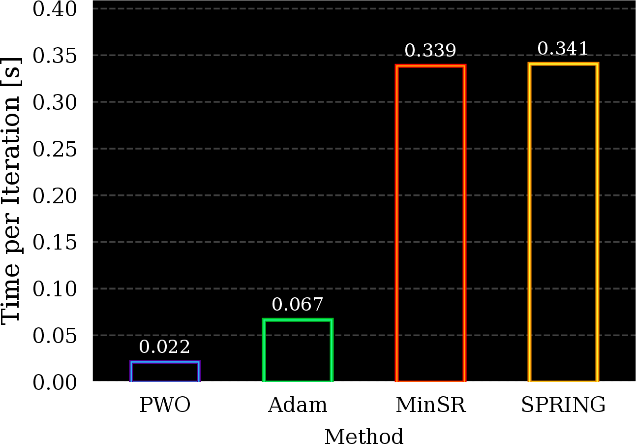

Figure 8: Per-iteration computational cost and normalized iteration speed for PWO and the baseline optimizers on the Heisenberg \(J_1\)–\(J_2\) chain with the default architecture 2.0.4.2. Both measurements are obtained on a single NVIDIA L40S GPU. Normalized speed is reported as the number of optimizer iterations per unit time relative to SPRING, so higher is faster.. a — Wall-clock time per optimizer iteration., b — Normalized iteration speed relative to SPRING.
Beyond convergence in wall-clock time, it is useful to isolate the computational cost of each optimization update. Figure 8 (b) compares the normalized iteration speed (optimization steps per unit of time) of PWO against the baselines. The speed advantage over minSR is expected: PWO is a first-order method and does not require constructing or inverting the stochastic-reconfiguration matrix. In contrast, minSR replaces the original \(P\times P\) SR solve by an \(M\times M\) solve, where \(M\) is the number of samples, but it still requires expensive Jacobian contractions and a matrix inversion or linear solve. PWO avoids this curvature computation entirely.
The comparison with Adam is more subtle. A single PWO update has additional bookkeeping relative to Adam, including probability ratios, clipping terms, and wrapped phase increments. However, in VMC the dominant cost is often not the optimizer algebra itself, but sampling configurations and evaluating the corresponding local energies. PWO computes local energies and advantages once for a sampled batch and then reuses that batch across multiple proximal inner epochs. Adam, in contrast, performs a single update per sampled batch, so the local-energy overhead is paid again for each parameter update. Thus, PWO can amortize the expensive energy computation across several optimization steps, making its effective per-update cost competitive with Adam despite the more structured surrogate objective.
2.0.3.3 Why RWKV?
RWKV is a particularly natural architecture for large-scale autoregressive NQS because it combines the expressivity of sequence models with recurrent inference. Unlike Transformer-based autoregressive models, RWKV does not require a growing key-value cache, so its per-token inference cost and memory footprint remain constant in the sequence length [18]. This is well aligned with autoregressive VMC, where spin configurations are generated sequentially and model evaluations are repeatedly invoked during Monte Carlo optimization. Recurrent architectures have also been successful in autoregressive NQS more broadly, where they provide exact independent sampling from the Born distribution while avoiding Markov-chain mixing issues [10], [16]. Finally, recent hyperscale RWKV fine-tuning work provides a practical implementation foundation for adapting billion-parameter recurrent models to nonstandard optimization objectives [48]. For these reasons, RWKV is a useful stress test for whether PWO can scale beyond conventional NQS architectures.
2.0.3.4 Limitations of PWO
Although PWO is supported by a first-order consistency result and a clipped improvement bound, the theory remains local and conservative: it relies on common-support and boundedness assumptions and does not imply global convergence for neural-network training. Empirically, our results include one-dimensional chains, a frustrated two-dimensional square lattice, and a large-scale RWKV fine-tuning experiment, but they are still not a comprehensive NQS benchmark across Hamiltonian families. In particular, broader validation on larger two-dimensional systems, fermionic models, and electronic-structure problems remains open. Finally, PWO introduces additional optimization hyperparameters, such as amplitude and phase clipping thresholds and the number of inner epochs, whose optimal values may depend on the Hamiltonian, ansatz, system size, and sample budget.
2.0.4 Experimental Details↩︎
2.0.4.1 Hyperparameter search
For each method, we perform a small hyperparameter search over the learning rate using a grid sweep and select the configuration with the best validation performance. For PWO, we additionally tune the clipping parameters that control the amplitude and phase surrogate objectives. Specifically, after selecting an initial learning rate, we independently grid search each clipping parameter while holding the best values found so far fixed. This sequential procedure provides a simple and computationally tractable way to tune the additional PWO-specific hyperparameters without requiring an exhaustive joint sweep over all combinations.
For Adam-based methods, including PWO, we use a cosine one-cycle learning-rate schedule [49]. The learning rate is first increased to a peak value during a short warmup phase and is then annealed smoothly to a small final value by cosine decay. The peak learning rate is selected by the grid search above, while the other schedule parameters are fixed across runs. For PWO, which performs multiple optimization epochs per sampled batch, we scale the transition horizon by the number of PPO epochs so that the schedule evolves on a comparable outer-iteration timescale. For minSR and SPRING, a constant learning rate performed better than scheduled variants.
Because the Heisenberg and J1–J2 chains are more challenging optimization problems than the transverse-field Ising model, we use longer learning-rate schedules for these settings (compare Appendices 2.0.4.3-2.0.4.5). In particular, we allocate more transition steps to the Heisenberg chain than to Ising, and more transition steps to J1–J2 than to Heisenberg. This gives the optimizer a longer annealing horizon on the harder Hamiltonians, while keeping the schedule structure fixed across problems. To improve readability, we report the method-specific hyper-parameters for each Hamiltonian separately. The Ising configuration is shown first, followed by the Heisenberg and J1–J2 settings in the subsequent subsections.
2.0.4.2 Neural Quantum State Architecture
Across experiments, we use the same autoregressive recurrent neural network for PWO and minSR, ensuring that performance differences arise from the optimizer rather than the parametrization. Given a spin configuration \(\vb{s}\in\{\pm1\}^N\), we map spins to binary tokens, prepend a beginning-of-sequence token, and embed the resulting sequence with learned token embeddings of dimension \(32\) and learned positional embeddings. The embedded inputs are projected to dimension \(256\), followed by a \(\tanh\) nonlinearity and layer normalization. The backbone consists of GRU layers with residual connections between recurrent blocks. From the shared recurrent representation, we use two separate two-layer MLP heads and GELU activations: an amplitude head, which outputs conditional log-probabilities via a log-softmax, and a phase head, which outputs bounded phases through a \(\tanh\) nonlinearity scaled by \(\pi\). The model has 1.4M parameters. Unless otherwise stated, all methods and Hamiltonians use the same architecture. The shared hyperparameters are summarized in Table 2.
| Architecture hyperparameter | Value |
|---|---|
| Token embedding dimension | \(32\) |
| Site embeddings | Learned |
| Backbone input dimension | \(256\) |
| Backbone nonlinearity | \(\tanh\) |
| Backbone normalization | Layer normalization |
| Recurrent backbone | GRU |
| Number of GRU layers | \(3\) |
| GRU hidden dimension | \(256\) |
| Amplitude head | 2-layer MLP |
| Phase head | 2-layer MLP |
| Head hidden dimension | \(256\) |
| Head activation | GELU |
| Phase output | \(\pi \tanh(\cdot)\) |
| Phase scale | \(\pi\) |
2.0.4.3 Ising Model
max width=
2.0.4.4 Heisenberg Chain
max width=
2.0.4.5 Heisenberg \(J_1\)–\(J_2\) Chain
max width=
2.0.4.6 Two-dimensional \(J_1\)–\(J_2\) square-lattice experiment
Using the same method hyper-parameters as above, we evaluate PWO on the frustrated spin-\(1/2\) \(J_1\)–\(J_2\) Heisenberg model on a two-dimensional square lattice, \[\begin{align} \hat{H}_{J_1\text{--}J_2}^{\mathrm{2D}} = J_1 \sum_{\langle i,j\rangle} \hat{\vb S}_i \cdot \hat{\vb S}_j + J_2 \sum_{\langle\langle i,j\rangle\rangle} \hat{\vb S}_i \cdot \hat{\vb S}_j , \end{align}\] where \(\langle i,j\rangle\) and \(\langle\langle i,j\rangle\rangle\) denote nearest- and next-nearest-neighbor pairs, respectively. We use an \(L\times L\) square lattice with \(L=10\), periodic boundary conditions, \(J_1=1\), and \(J_2=0.5\). All runs are restricted to the zero-magnetization sector, \(S^z_{\mathrm{tot}}=0\), by masking infeasible autoregressive choices during sampling and evaluation.
For this experiment we use a complex-valued patch-autoregressive transformer designed for two-dimensional lattices. Instead of generating spins one at a time, the model partitions the \(10\times 10\) lattice into non-overlapping \(2\times 2\) patches. Each patch is represented as a categorical token with vocabulary size \(2^4=16\), so the full configuration is generated as a sequence of \[\begin{align} T = \left(\frac{L}{2}\right)^2 = 25 \end{align}\] autoregressive tokens. The wavefunction is factorized over patch tokens as \[\begin{align} \log \psi_\theta(\vb s) = \sum_{t=1}^{T} \left[ \frac{1}{2}\log p_\theta(a_t \mid a_{<t}) + i\,\phi_\theta(a_t \mid a_{<t}) \right], \end{align}\] where the factor \(1/2\) corresponds to the Born-rule convention \(P_\theta(\vb s)=|\psi_\theta(\vb s)|^2\).
The model prepends a beginning-of-sequence token and embeds patch tokens with learned token embeddings of dimension \(64\). We also use learned site embeddings and prefix-count features that encode the partial magnetization constraint. These embeddings are projected to width \(96\), normalized with layer normalization, and passed through an \(8\)-layer causal transformer backbone. Each transformer block uses \(6\) attention heads, two-dimensional axial RoPE with base \(100\), residual connections, and a feedforward width of \(4\times 96=384\).
From the final transformer representation, the model uses separate amplitude and phase heads. Both heads are two-layer MLPs with hidden dimension \(192\) and GELU activations. The amplitude head outputs masked conditional log-probabilities through a log-softmax, ensuring exact normalization over feasible patch choices. The phase head outputs centered phase increments using a \(\pi\tanh(\cdot)\) parameterization, with small initialization scale \(10^{-3}\). This gives an exactly sampleable complex autoregressive neural quantum state adapted to the two-dimensional square lattice.
While the aim of this experiment is to compare optimizers and not to achieve the state-of-the-art variational energy (around -199.0536 [37]), we note that the energy of the PWO-trained autoregressive transformer of 1.5M parameters is \(-185\) after 30 mins, reaches \(-195.6\) after 24 hours, and keeps decreasing. The run is on a single GPU and imposes no symmetries, except for zero-magnetization sampling.
max width=
2.0.4.7 Scaling Experiment
To study how performance scales with model capacity, we train three model sizes on the frustrated Heisenberg \(J_1\)–\(J_2\) chain (\(N=12\), \(J_1=1\), \(J_2=0.5\), periodic boundary conditions) using PWO, Adam, and minSR. All three sizes share the same autoregressive GRU architecture described in Appendix 2.0.4.2; they differ only in the number of recurrent layers and hidden dimensions. Table 3 summarises the sizes and the corresponding total parameter counts.
| Size | GRU layers | RNN hidden | Head hidden | Parameters |
|---|---|---|---|---|
| Tiny | 1 | 64 | 64 | \(44{,}452\) |
| Small | 2 | 128 | 128 | \(269{,}156\) |
| Medium | 3 | 256 | 256 | \(1{,}456{,}356\) |
The hyperparameters used for each optimization method in the scaling experiment are listed in Table ¿tbl:tab:scaling95hyperparams?. The schedule and clipping parameters are identical to those of the main \(J_1\)–\(J_2\) experiments (see Tables ¿tbl:tab:j1j295hyperparams? and 2); only the number of transition steps differs to account for the change in model size.
max width=
2.0.4.8 RWKV-7 on Ising Model
max width=
2.0.5 Additional Figures↩︎
2.0.5.1 Individual Seed Plots for All Hamiltonias
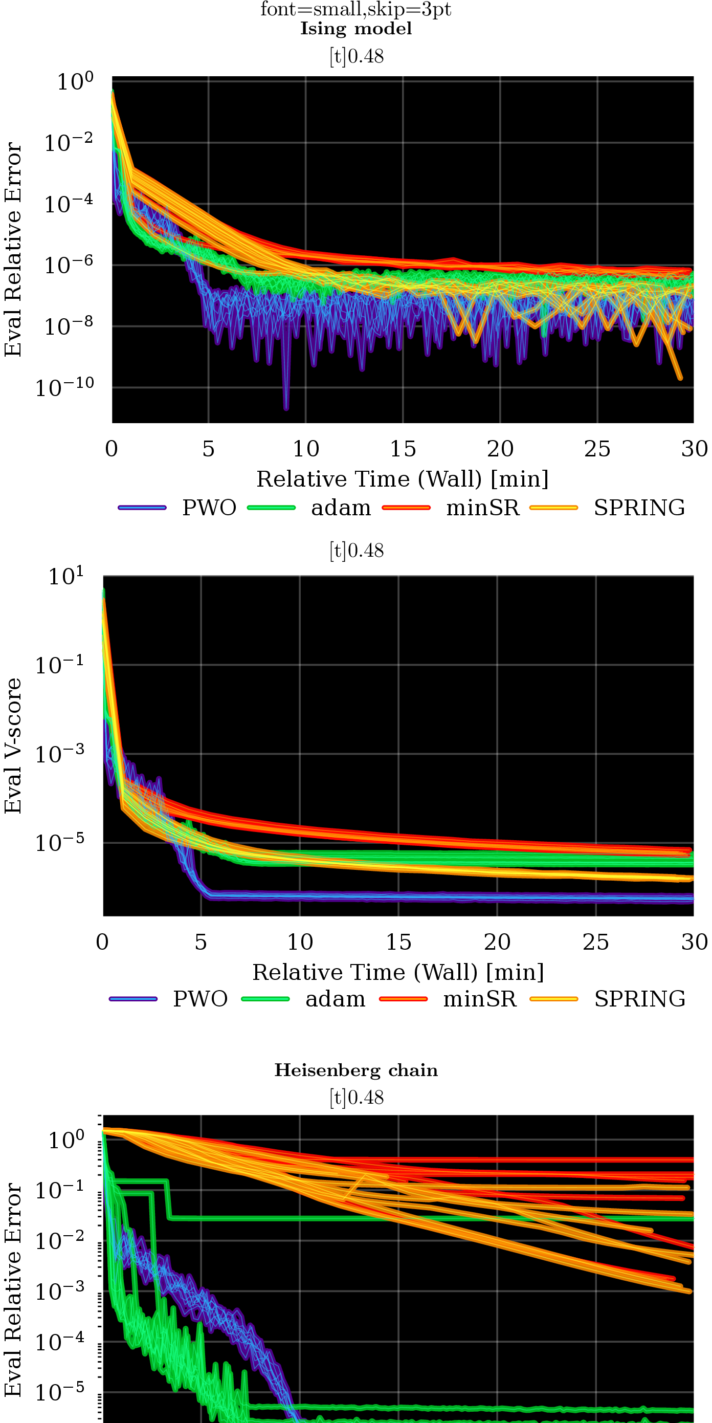
2.0.5.2 Scaling Samples and System Sizes
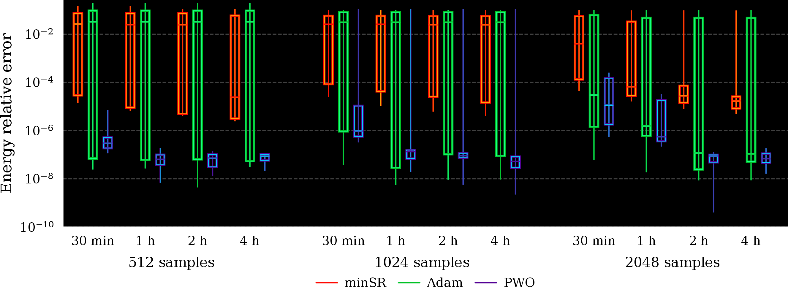
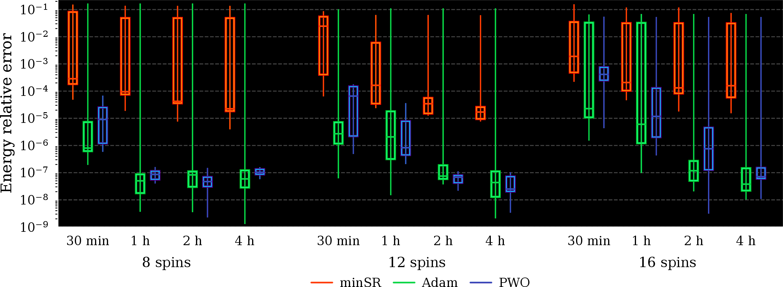
2.0.5.3 Individual Seed Plots for RWKV7 Fine-tuning


Figure 12: Individual-seed fine-tuning curves for the \(1.5\)B-parameter RWKV-7 neural quantum state on the transverse-field Ising model. Each curve corresponds to one random seed, with relative error shown on the left and V-score on the right. PWO consistently remains stable across seeds and reaches lower final error and variance than the Adam baseline, indicating that the proximal objective improves robustness even in the billion-parameter regime..