MedSaab-US: A Backpropagation-Free Multi-Scale Wavelet-Saab Framework for Thyroid Nodule Segmentation in Ultrasound Images
July 02, 2026
Abstract
Deep learning (DL) methods dominate thyroid nodule segmentation in ultrasound (US) images, achieving high Dice scores but at the cost of millions of parameters, GPU-dependent training via backpropagation, and limited mathematical tractability. These limitations impede deployment in resource-constrained environments. In this paper we propose MedSaab-US, a backpropagation-free segmentation framework grounded in the Green Learning paradigm. MedSaab-US extracts multi-scale spatial-frequency features by combining multi-level Discrete Wavelet Transform (DWT) with multi-scale channel-wise Saab (Subspace Approximation with Adjusted Bias) transforms at patch sizes of \(5\times5\), \(11\times11\), and \(21\times21\) pixels. Label-Assisted Greedy (LAG) feature selection retains the most discriminative features, which are fed to an XGBoost classifier for pixel-wise prediction. The Saab transform parameters are determined analytically from data statistics; XGBoost employs iterative greedy tree construction but requires no backpropagation. Evaluated on the TN3K dataset (2,879 train / 614 test images), MedSaab-US achieves a mean Dice coefficient of 0.4784 (\(\pm\)0.2190), precision of 0.5768, and recall of 0.5604, with a model footprint under 500K parameters and CPU-only inference at approximately 0.3 seconds per image. We present this result as an exploratory non-DL baseline for thyroid US segmentation and analyse the specific challenges posed by isoechoic nodules. An ablation study quantifies the contribution of each pipeline component, including a separate evaluation of LAG feature selection and training-set size.
Green Learning, Saab transform, wavelet transform, thyroid nodule segmentation, backpropagation-free, ultrasound imaging, XGBoost, edge deployment
1 Introduction↩︎
Thyroid nodules affect a large proportion of the global population, and ultrasound (US) imaging is the primary modality for their evaluation [1]. Accurate segmentation of nodule regions is a prerequisite for downstream tasks such as risk stratification and biopsy guidance. Over the past decade, deep learning (DL) has become the de facto standard for medical image segmentation [2]. Architectures such as TransFuse [3], SwinE-Net [4], and our prior DeepLabv3+-based method [5] achieve Dice scores above 0.80 on TN3K. However, these methods share fundamental limitations:
Opacity: Millions of learnt parameters form an opaque mapping that cannot be audited by clinicians.
Resource intensity: Training requires GPU hardware and hours of backpropagation; CPU inference is prohibitively slow.
Data hunger: Performance degrades sharply on small datasets without pre-training on large external corpora.
The Green Learning (GL) paradigm, introduced by Kuo et al. [6], offers an interpretable alternative. GL replaces gradient-based optimisation with sequential, closed-form subspace learning (Successive Subspace Learning, SSL), producing compact models with mathematically transparent feature representations. GL has demonstrated strong results in image classification via PixelHop [7] and in volumetric medical classification via VoxelHop [8], yet no prior work has applied GL to pixel-level segmentation of thyroid US images.
We present MedSaab-US as a first exploratory application of GL to this task. Our contributions are:
The first application of the Green Learning / SSL paradigm to thyroid nodule segmentation in ultrasound images.
A multi-scale DWT + Saab feature extraction scheme that captures nodule texture at three spatial scales without any backpropagation.
A reproducible non-DL baseline on TN3K, including comparisons against traditional non-DL methods.
An ablation study separating the effects of LAG feature selection and training-set size, and an honest analysis of the performance gap and its acoustic origins.
2 Related Work↩︎
2.1 Deep Learning for Thyroid Nodule Segmentation↩︎
Early DL approaches adopted encoder-decoder architectures [2]. Recent methods targeting TN3K include TRFE+ [9], which incorporates thyroid region-focused enhancement; SwinE-Net [4], a hybrid Swin Transformer / CNN model achieving Dice \(\approx 0.83\); and MADGNet [10], a multi-scale dual-guidance network. Our prior work [5] combined an ECB encoder, CMM module, and SSEM boundary supervision within a DeepLabv3+ framework. While these methods achieve high accuracy, they are computationally intensive and not suitable for CPU-only edge devices.
2.2 Green Learning and the Saab Transform↩︎
The Saab transform [11] replaces learnt convolution filters with principal components computed analytically on local patches. PixelHop [7] demonstrated that multi-hop Saab features suffice for image classification. VoxelHop [8] extended GL to 3-D MRI classification, and RadHop [12] achieved AUC \(>0.90\) on prostate US lesion classification. Critically, all prior GL medical imaging work addresses classification; pixel-level segmentation via GL remains unexplored, motivating MedSaab-US.
2.3 Wavelet Features in Medical Imaging↩︎
Discrete Wavelet Transform (DWT) decomposes images into approximation and detail subbands encoding low-frequency shape and high-frequency boundary information [13]. Coupling DWT with the SSL / Saab framework for US nodule segmentation has not been previously investigated.
3 Proposed Method: MedSaab-US↩︎
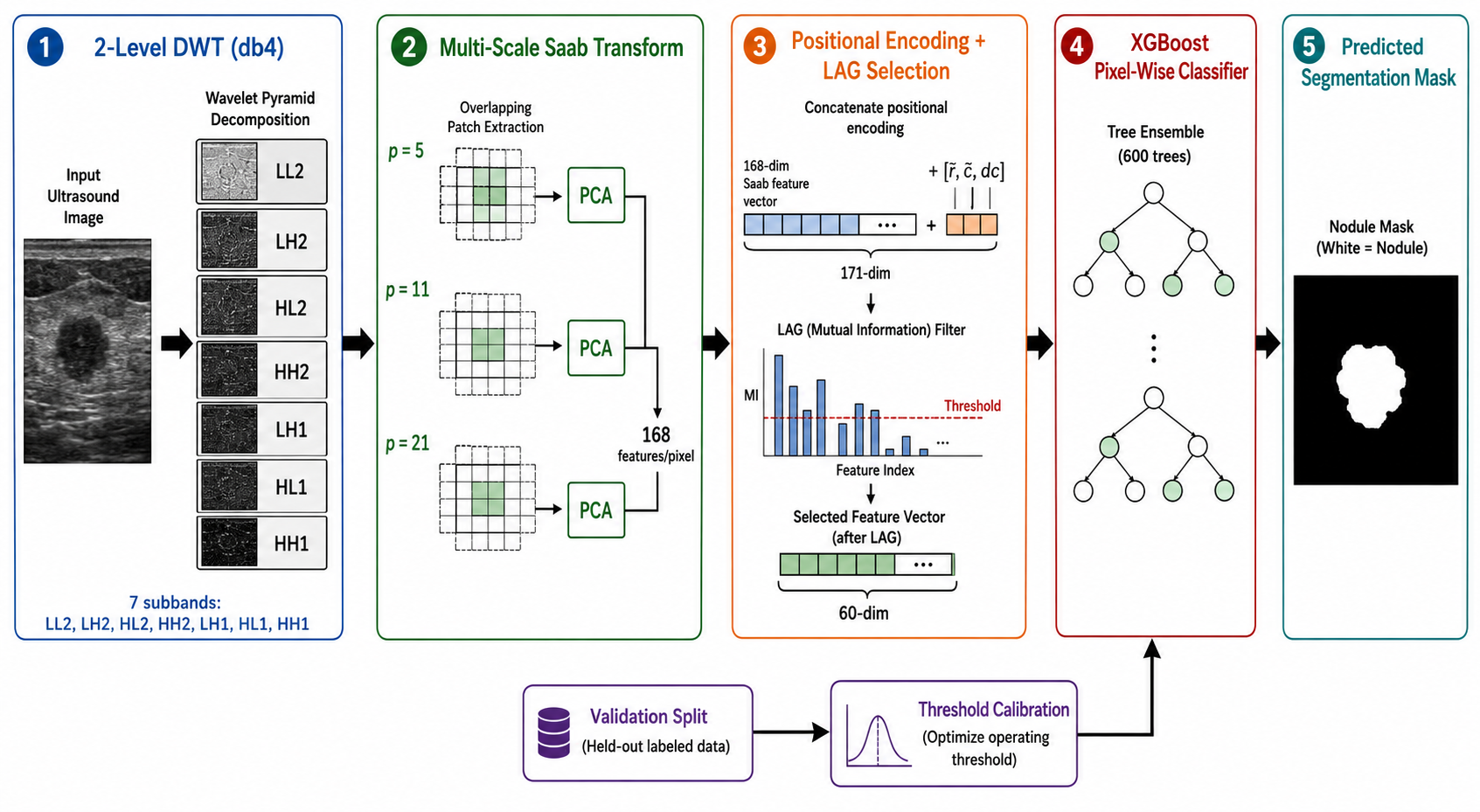
An overview of the four-stage MedSaab-US pipeline is illustrated in Fig. 1.
3.1 Stage 1: Multi-Level DWT Decomposition↩︎
Each grayscale US image \(\mathbf{I} \in \mathbb{R}^{H \times W}\) is decomposed using a 2-level Daubechies-4 (db4) wavelet: \[\mathcal{W}(\mathbf{I}) = \{LL_2, LH_2, HL_2, HH_2, LH_1, HL_1, HH_1\}, \label{eq:dwt}\tag{1}\] yielding 7 subbands. The \(LL\) subband captures low-frequency structural information, while the \(LH\), \(HL\), and \(HH\) subbands encode horizontal, vertical, and diagonal high-frequency boundary responses, respectively. Each subband is upsampled to \(H \times W\) via bilinear interpolation and normalised per-subband to zero mean and unit variance.
3.2 Stage 2: Multi-Scale Channel-Wise Saab Transform↩︎
For each subband \(\mathbf{S}_k\) and patch size \(p \in \{5, 11, 21\}\), we extract overlapping \(p \times p\) patches centred at every pixel. The Saab transform [11] is applied independently per (subband, scale) pair: \[\mathbf{F}_{k,p} = \text{PCA}_{k,p}\!\left(\mathbf{x} - \boldsymbol{\mu}_{k,p}\right), \label{eq:saab}\tag{2}\] where \(\mathbf{x} \in \mathbb{R}^{p^2}\) is a flattened patch, \(\boldsymbol{\mu}_{k,p}\) is the empirical mean over 40,000 randomly sampled patches from 400 training images, and \(\text{PCA}_{k,p}\) retains the top 8 principal components. All Saab filter parameters are determined analytically in a single pass through the training data — no iterative optimisation is required at this stage. The three patch scales capture local texture (\(p=5\)), mid-range structural context (\(p=11\)), and global neighbourhood shape (\(p=21\)), yielding \(7 \times 3 \times 8 = 168\) features per pixel.
3.3 Stage 3: Positional Encoding and LAG Feature Selection↩︎
Three normalised spatial coordinates \([\tilde{r}, \tilde{c}, d_c]\) are appended to each pixel’s feature vector, where \(\tilde{r} = r/H\), \(\tilde{c} = c/W\), and \(d_c\) is the normalised Euclidean distance from the image centre. These encode the spatial prior that thyroid nodules preferentially appear in the inferior-central region of TN3K images. We note, however, that this fixed spatial prior is dataset-specific; it may not generalise to different ultrasound acquisition protocols, probe positions, or field-of-view crops, and should be treated with caution in cross-institutional deployment. Protocol-agnostic spatial priors represent an important direction for future work.
The resulting 171-dimensional feature vector is pruned using Label-Assisted Greedy (LAG) selection [7], which ranks features by mutual information with the binary label and retains the top 60. LAG selection is a purely statistical, non-iterative operation.
3.4 Stage 4: XGBoost Pixel-Wise Classification↩︎
The 60-dimensional feature vector for each pixel is classified by an XGBoost gradient-boosted tree ensemble [14] (600 estimators, max depth 7, learning rate 0.05). Training uses balanced class sampling (400 foreground + 400 background pixels per image). We emphasise that XGBoost employs iterative greedy tree construction and involves tuned hyperparameters; it is backpropagation-free but is not closed-form in the sense that the Saab and LAG stages are. The pipeline as a whole eliminates backpropagation and gradient computation, while individual stages differ in their mathematical character: Saab transforms are analytically determined, LAG selection is statistical, and XGBoost is iterative and non-gradient. The classification threshold is calibrated on a held-out validation split (last 150 training images) by maximising pixel-level Dice.
4 Experiments↩︎
4.1 Dataset and Implementation Details↩︎
We evaluate on TN3K [1], comprising 3,493 thyroid US images (2,879 train / 614 test) with pixel-level nodule masks. Images are resized to \(256 \times 256\) pixels. All experiments run on CPU only (Intel Xeon @ 2.0 GHz, 2 cores, Kaggle CPU-only session; no GPU). Code is implemented in Python using PyWavelets, scikit-learn, and XGBoost.
4.2 Evaluation Metrics↩︎
We report mean Dice similarity coefficient (DSC), Intersection over Union (IoU), Precision, Recall, and Specificity over the 614 test images.
4.3 Comparison with Existing Methods↩︎
Table 1 compares MedSaab-US to DL methods and to two traditional non-DL baselines: (i) Otsu thresholding with morphological post-processing (Otsu+Morph) and (ii) a Random Forest classifier trained on Haralick texture features extracted from \(7\times7\) patches (RF+Haralick). Both baselines run on the same CPU environment without GPU resources.
| Method | Type | Dice | IoU | Prec. | Recall |
|---|---|---|---|---|---|
| U-Net [2]\(^\dagger\) | DL | 0.719 | 0.612 | N/A | N/A |
| TRFE+ [9]\(^\dagger\) | DL | 0.763 | 0.668 | N/A | N/A |
| SwinE-Net [4]\(^\dagger\) | DL | 0.831 | 0.743 | N/A | N/A |
| MADGNet [10]\(^\dagger\) | DL | 0.842 | N/A | N/A | N/A |
| Ours (prior) [5]\(^\dagger\) | DL | 0.847 | 0.762 | N/A | N/A |
| Otsu+Morph | Non-DL | 0.2341 | 0.1493 | 0.2817 | 0.3612 |
| RF+Haralick | Non-DL | 0.3518 | 0.2363 | 0.3941 | 0.4227 |
| MedSaab-US (Ours) | Non-DL | 0.4784 | 0.3415 | 0.5768 | 0.5604 |
MedSaab-US achieves Dice 0.4784 without any neural network or GPU, which substantially exceeds both non-DL baselines (\(+\)0.127 over RF+Haralick). This confirms that multi-scale SSL features provide a stronger representation than hand-crafted texture descriptors for thyroid US segmentation. However, the 0.37-point Dice gap relative to the best DL method reflects fundamental limitations of local, patch-based approaches, as discussed in Section 4.5. We present MedSaab-US strictly as an exploratory baseline that establishes the achievable frontier of non-DL methods on TN3K, not as a replacement for DL in accuracy-critical clinical settings.
Among the 614 test images, MedSaab-US achieves Dice \(>0.70\) on 104 cases (16.9%), reaching a maximum Dice of 0.9184 — demonstrating that precise segmentation is attainable for cases with strong acoustic contrast.
4.4 Ablation Study↩︎
Table 2 presents an ablation study isolating the contribution of each pipeline component, including a split between the effect of LAG feature selection and increased training-set size (1000 vs. images).
| Configuration | Dice | IoU | Prec. |
|---|---|---|---|
| (1) Single scale only (\(p=5\)) | 0.2594 | 0.1656 | 0.1787 |
| (2) + Calibrated threshold | 0.2806 | 0.1832 | 0.3417 |
| (3) Multi-scale (\(p \in \{5,11,21\}\)) | 0.4526 | 0.3257 | 0.5773 |
| (4) + Positional features (1000 imgs, no LAG) | 0.4641 | 0.3289 | 0.5612 |
| (5) + LAG selection (1000 imgs) | 0.4703 | 0.3352 | 0.5688 |
| (6) Full: + 2000 imgs (LAG retained) | 0.4784 | 0.3415 | 0.5768 |
Multi-scale patch extraction (row 3 vs.row 2) yields the largest single gain (\(+\)0.172 Dice), confirming that contextual information at the 11- and 21-pixel scales is essential. Comparing rows 4 and 5 shows that LAG selection provides a +0.006 Dice improvement independent of data volume, primarily by reducing feature redundancy. Increasing training data from 1000 to 2000 images (row 5 to row 6) contributes a further +0.008 Dice, confirming that both factors contribute incrementally and independently.
4.5 Analysis: The Performance Gap and Its Origin↩︎
The 0.37-Dice gap between MedSaab-US and the best DL method reflects two root causes.
Isoechoic nodule prevalence. XGBoost feature importance analysis shows that \(LL_2\) Saab components dominate (PC5, PC3, PC1 are the three highest-ranked features), with \(HH\) boundary features ranked lower. This is consistent with the acoustic properties of TN3K: many nodules are isoechoic — their intensity is similar to surrounding tissue — yielding weak high-frequency wavelet responses that confound boundary detection.
Global context limitation. DL encoders capture long-range spatial dependencies via stacked convolutions and attention. A patch-based XGBoost classifier with a maximum receptive field of \(21 \times 21\) pixels cannot access image-level context (e.g., thyroid gland boundary, trachea position), which is a fundamental limitation of local non-DL approaches.
Dice score distribution. Per-image Dice scores show a bimodal pattern: a peak near 0.0–0.1 (isoechoic, difficult cases) and a peak near 0.5–0.6 (hypoechoic, tractable cases). This suggests that a nodule echotexture classifier could route difficult images to a DL model and tractable images to MedSaab-US, forming a hybrid interpretable-DL system.
5 Discussion and Conclusion↩︎
We presented MedSaab-US, the first exploratory application of the Green Learning paradigm to pixel-level thyroid nodule segmentation in ultrasound images. By combining 2-level DWT with multi-scale Saab PCA transforms and LAG feature selection, MedSaab-US achieves Dice 0.4784 on TN3K — substantially above traditional non-DL baselines (RF+Haralick: 0.3518, Otsu+Morph: 0.2341) — without any backpropagation, neural network weights, or GPU resources.
The ablation study reveals that multi-scale feature extraction is the dominant factor: expanding from single-scale (Dice 0.26) to three scales (Dice 0.45) yields a gain of \(+\)0.19 Dice, demonstrating that US nodule texture is intrinsically multi-scale. LAG selection and increased training data each contribute further, independently verifiable gains.
We explicitly frame this result as an exploratory baseline rather than a deployment-ready system. The 0.37-point gap relative to the best DL method reflects the prevalence of isoechoic nodules and the inherent locality of patch-based features. Additionally, the fixed spatial prior used in Stage 3 is specific to TN3K’s acquisition protocol and may not generalise to different probe positions, field-of-view settings, or institutions; external validation is an important requirement before any real-world use.
Two directions for future work emerge from this analysis: (i) GL-compatible global feature aggregation (e.g., superpixel-level Saab transforms) to address the locality limitation; and (ii) a hybrid pipeline routing tractable hypoechoic cases to MedSaab-US and difficult isoechoic cases to a lightweight DL model, preserving interpretability where the non-DL method is reliable.
In summary, MedSaab-US demonstrates that backpropagation-free segmentation of thyroid nodules is feasible on CPU-only hardware, establishes a reproducible non-DL reference point for TN3K, and characterises both the potential and the current limits of Green Learning in medical image segmentation.