X-Splat: Gaussian Splatting for 3D CBCT Generation
from Single Panoramic Radiograph
July 02, 2026
Generating a 3D dental volume from a single panoramic radiograph (PXR) could provide a low-radiation alternative to Cone-Beam Computed Tomography (CBCT), but the problem is highly underdetermined: panoramic acquisition integrates 3D attenuation along
curved X-ray paths into a 2D image, leaving depth-resolved anatomy unobserved. Existing implicit and generative approaches often produce oversmoothed geometry or anatomically inconsistent hallucinations, lacking geometry-driven supervision and relying on
smooth representations unable to precisely localize sharp anatomical boundaries. We propose X-Splat, the first Gaussian Splatting framework for generating CBCT-like 3D dental volumes from a single PXR. X-Splat uses the known panoramic acquisition geometry
as a generation scaffold: learnable anisotropic Gaussian primitives are initialized along the X-ray paths that formed the input image and adjusted in a single feed-forward pass, constrained by Beer–Lambert reprojection and multi-view radiographic training
supervision. A lightweight residual refiner adds dataset-level anatomical priors without overriding the geometry already resolved by the Gaussians. We train on synthetic PXR–CBCT pairs, enabling direct volumetric supervision without paired real scans. We
further introduce segmentation-based geometry-aware metrics, providing the first evaluation of PXR-based generation over maxillofacial anatomy. X-Splat outperforms NeRF- and GAN-based baselines, recovering individual teeth, cortical boundaries, and
alveolar structure, including the mandibular canal which prior methods fail to reconstruct. Code will be available at github.com/X-Splat.
1 Introduction↩︎
Inferring 3D anatomy from 2D projections is a fundamental problem across imaging science, physics, and computer vision, with particular clinical importance in dentistry, where Cone-Beam Computed Tomography (CBCT) remains the standard for 3D
maxillofacial imaging by acquiring hundreds of 2D projections over a full arc to reconstruct a sub-millimetre attenuation volume [1]. Its
diagnostic superiority over 2D imaging is well established, from detecting cortical destruction and root resorption to depicting the relationship between molar roots and the mandibular canal [2]. Yet CBCT is acquired only when clinically indicated, whereas panoramic radiography (PXR) is widely available, low-cost, and substantially lower in radiation dose [3], [4]. Consequently, routine dental care often produces longitudinal
archives of panoramic images, while CBCT data remain comparatively sparse. Inferring a CBCT-like volume from a single PXR would extend 3D dental analysis to large retrospective panoramic-image archives and to settings where CBCT is unavailable [5], [6]. However, the problem is a highly underdetermined
inverse problem: a panoramic projection integrates 3D attenuation along rays into a single 2D image, leaving depth-resolved anatomy unobserved (Fig.1). Unlike sparse-view CT, where multiple projections constrain
depth [7]–[9], generating a 3D volume from a single-view
requires strong anatomical and geometric priors as necessary constraints.

Existing PXR-to-3D methods [10]–[15] leave three gaps that motivate our work. First, they rely on convolutional encoder-decoders or implicit neural fields that represent the volume as a dense grid or continuous scalar field; such representations are smooth
by construction and systematically under-resolve the sharp interfaces, such as root boundaries, cortical bone surfaces, and the mandibular canal cortex, that carry the most diagnostic value. Implicit paradigms like NeRF [16] sample at fixed intervals along each ray and cannot adapt to anatomical structure, while GAN-[17], [18] and diffusion-based [19], [20] generators risk anatomically inconsistent hallucinations and often remain computationally
prohibitive at CBCT resolution. Second, prior methods either require additional input beyond the PXR, such as dental arch curves [10], or produce
volumes from a single image that are locally plausible but globally inconsistent with real dental topology. Third, evaluation remains dominated by intensity-based metrics such as SSIM and PSNR, sometimes with coarse global Dice Score [11]; recent sparse-view studies show these aggregate voxel errors without reflecting whether clinically relevant structures are correctly recovered, so substantial
structural inaccuracy can pass unnoticed [21]. A detailed review of related work is provided in Appendix 5.
To address these limitations, we propose X-Splat, a Gaussian Splatting framework for single-view 3D CBCT-like volumes from a panoramic radiograph. We formulate single-PXR 3D dental volume estimation as geometry-constrained
generation: unlike tomographic reconstruction, which resolves depth from multiple projections, a single PXR leaves the volume underdetermined, requiring conditional generation under strong geometric priors. Rather than a smooth implicit field, we
represent the volume with localized anisotropic 3D Gaussian primitives [22] whose explicit geometry naturally encodes sharp boundaries and can be
optimized via physics-consistent radiative rendering aligned with the Beer–Lambert attenuation model [23], [24]. Gaussians are initialized along panoramic acquisition rays and predicted in a feed-forward pass, then displaced, rotated, and anisotropically scaled to follow anatomical boundaries and
fill the space between sparsely separated rays (Fig.1D). Finally, we evaluate generated volumes’ quality using a ToothFairy3-trained segmentation network [25]–[29] to derive geometry-aware metrics over individual teeth, the mandibular canal (MC), and the five major maxillofacial structures, providing a more faithful assessment of structural fidelity than intensity measures alone.
Our main contributions are as follows:
We propose X-Splat, the first Gaussian Splatting framework for generating CBCT-like 3D dental volumes from a single panoramic radiograph. Explicit anisotropic Gaussian primitives, constrained by Beer–Lambert reprojection and multi-view radiographic supervision, provide a geometry-grounded alternative to the smooth implicit fields and dense voxel decoders of prior PXR-to-3D methods.
From a single PXR alone, X-Splat recovers fine dental and maxillofacial structures that existing methods systematically miss, including individual tooth roots, cortical boundaries, and the mandibular canal. This is enabled by a ray-anchored Gaussian representation in which a shared feed-forward network predicts each primitive’s displacement, orientation, scale, and density using the known panoramic acquisition geometry as an acquisition scaffold.
We combine geometry-driven Gaussian generation with a lightweight residual refiner constrained by multi-view DRR supervision, adding dataset-level anatomical detail while keeping the generated volume tied to the input projection. We further introduce geometry-aware structural metrics beyond conventional image-quality measures, evaluating recovery of individual teeth, cortical boundaries, alveolar structure, and the mandibular canal.
2 Methods↩︎
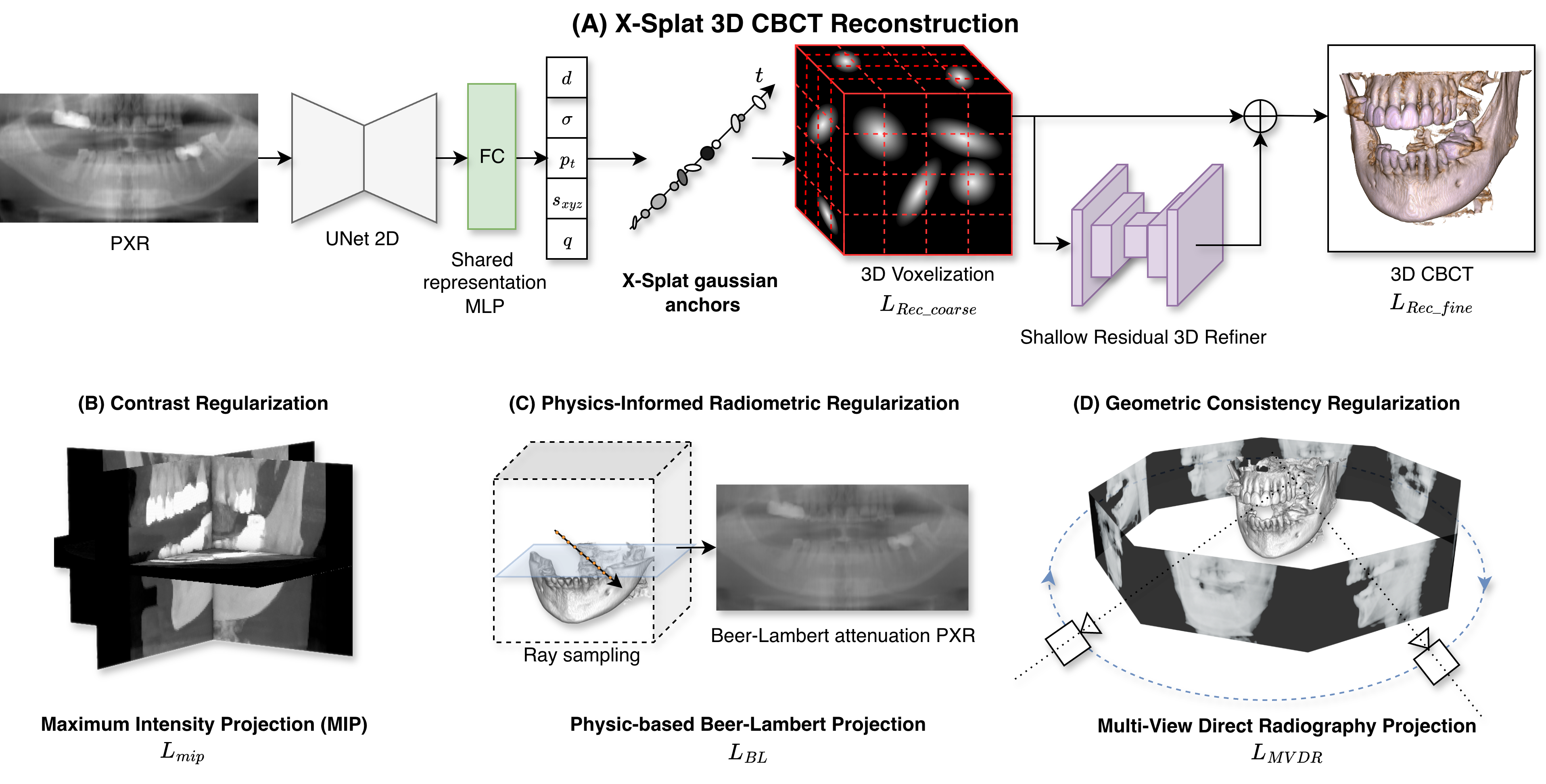
We design X-Splat using three complementary choices. (i) Geometry-anchored initialization: we exploit the known panoramic acquisition geometry, anchoring 3D Gaussian primitives along the predefined ray trajectories that map 2D pixels to 3D space, concentrating capacity where the input is informative without per-scene optimization. (ii) Feed-forward prediction and refinement: a 2D U-Net encoder and a single MLP, shared across all Gaussian attributes and anchors, predict all Gaussian parameters from the input and each anchor’s positional encoding; the Gaussians are rasterized into a coarse volume, which a lightweight 3D residual U-Net refines, adding population-level anatomical priors as a small correction that keeps the output tethered to the input. (iii) Multi-view consistency: during training, additional azimuthal projections supervise the volume, contracting the feasible set toward anatomically consistent solutions. Figure 2 illustrates the pipeline; the following subsections detail each component.
2.1 Problem Formulation↩︎
Let \(\mathbf{I} \in \mathbb{R}^{H_p \times W_p}\) denote a simulated panoramic X-ray (SimPX) rendered from a ground-truth CBCT volume \(V^* \in \mathbb{R}^{H \times W \times D}\) using the panoramic ray geometry and effective Beer–Lambert rendering convention of NeBLa [11]. This provides a calibrated computational forward model of panoramic image formation in which scanner-dependent spectral and intensity effects are absorbed into effective attenuation and rendering parameters. For a ray \(\mathbf{r}(t)\), the projected intensity is:
\[\mathcal{F}(V,\theta)(h,w) = \frac{1 - I_0\,\exp\!\Bigl(-\beta\sum_k \mu_k\,\Delta s\Bigr)}{p_{\max}}, \label{eq:beer95lambert}\tag{1}\]
where \(\mu_k\) denotes the effective attenuation at sample \(k\) along the ray, \(\Delta s\) is the voxel step size, and \(I_0\), \(\beta\), and \(p_{\max}\) are calibrated rendering constants. The inverse problem is to recover \(\hat{V}\) from a single observation \(\mathbf{I} = \mathcal{F}(V^*,\theta_0)\).
2.2 SimPX Ray Geometry↩︎
We adopt the SimPX synthesis pipeline and focal-trough ray geometry from NeBLa [11]. The panoramic focal trough is modelled by a quadratic curve \(f(x) = 0.01(x \pm 100)^2\), where \(x\) denotes horizontal coordinate in the axial CBCT slice, that defines 21 rotation centers: (see Fig.1 (A)) \(\mathbf{c}_i\), \(i=0,\ldots,20\), placed on the axial plane of a \(256\!\times\!256\) CBCT slice. At each centre \(\mathbf{c}_i\), rays are rotated by an angle \(\theta_i\) that varies with the dental region (denser near the molars) to simulate the variable angular sweep of a real panoramic scanner. Along each ray, \(K=200\) points are uniformly sampled within the volume boundary and rendered to a single pixel via Eq. 1 . The resulting SimPX has \(H_p\) rows (one per CBCT slice in \(Z\)) and \(W_p\) columns equal to the total number of rays, producing a 2D image whose pixels map to known 3D ray trajectories. This explicit ray-pixel correspondence is the geometric prior that X-Splat exploits for anchor placement, as described next.
2.3 Gaussian Anchor Initialization↩︎
The ray geometry provides a uniquely informative spatial prior. Every pixel \((h,w)\) of the SimPX corresponds to a known 3D ray \(\mathbf{r}_{h,w}(t)\), and the pixel intensity encodes the integrated attenuation along that ray. Rather than learning anchor positions from scratch through adaptive densification, we exploit this prior directly: we place one Gaussian anchor per ray sample, yielding \(N_g \approx 6\mathrm{M}\) anchors \(\{\mathbf{p}_j\}_{j=1}^{N_g}\) that densely cover the dental arch and jaw region from the outset. This concentrates representational capacity where the input is informative, avoiding the costly exploration phase that unconstrained Gaussian methods require.
2.4 3D Gaussian Splatting↩︎
Shared MLP. A single MLP \(f_\phi\), shared across all \(N_g\) anchors, predicts each Gaussian’s displacement, scale, rotation, and density in one forward pass. We extend the MLP conditioning scheme of NeBLa [11], combining global image features with per-point positional encoding, to the Gaussian Splatting domain. Per-scene optimization methods solve these jointly through iteration with adaptive densification and non-uniform learning rates per attribute [22], [24]; our feed-forward setting must resolve all parameters simultaneously and uniformly from the input image alone. Sharing weights across anchors is key: rather than predicting each attribute through separate heads, the network builds joint inductive biases over the full anatomy, since tissue of a given density at a given location implies a characteristic scale and orientation, which would be underexploited with a multi-head design. The MLP predicts:
\[(\hat{\delta t}_j,\; \mathbf{s}_j,\; \mathbf{q}_j,\; \alpha_j) = f_\phi\!\left(\mathbf{F}(\mathbf{p}_j) + \mathrm{PE}(\mathbf{p}_j)\right), \label{eq:mlp}\tag{2}\]
where \(\mathbf{F}(\mathbf{p}_j)\) are UNet features read directly at the pixel location on ray corresponding to anchor \(\mathbf{p}_j\) in the SimPX, \(\mathrm{PE}(\mathbf{p}_j)\) is the positional encoding, \(\hat{\delta t}_j\) is a raw scalar displacement, \(\mathbf{s}_j\in\mathbb{R}^3\) the log-scale, \(\mathbf{q}_j\in\mathbb{R}^4\) a unit quaternion, and \(\alpha_j\) the density.
Constrained axial-plane movement. Each Gaussian is permitted to move only along its anchor ray within the axial (XY) plane. This constraint is motivated by the structure of the SimPX: because rays run perpendicular to the dental arch and the CBCT is sampled slice-by-slice along \(Z\), allowing inter-slice (\(Z\)-axis) Gaussian migration would corrupt the dense axial coverage. The scalar displacement is bounded by \(\delta t_j = \tanh(\hat{\delta t}_j)\cdot\delta t_{\max}\), where \(\delta t_{\max} = 32\;\text{vox}\), and projected onto a 3D offset via the ray’s axial unit direction \(\hat{\mathbf{d}}_{w_j}\in\mathbb{R}^2\):
\[\Delta\mathbf{p}_j = \Bigl[\delta t_j\cdot\frac{\hat{\mathbf{d}}_{w_j}}{\mathbf{h}_{XY}},\;0\Bigr], \label{eq:delta95xyz}\tag{3}\]
where \(\mathbf{h}_{XY}=[H/2,\,W/2]\) maps voxel displacement to the \([-1,1]^3\) coordinate system and the zero \(Z\)-component enforces the no-inter-slice constraint. The final Gaussian centre is \(\tilde{\mathbf{p}}_j = \mathbf{p}_j + \Delta\mathbf{p}_j\).
Axial-plane rotation. Gaussian rotation is restricted to the axial plane (rotation around the superior-inferior \(Z\)-axis), again to prevent cross-slice interference and to keep each Gaussian’s spatial footprint aligned with its ray.
Scale initialization and clamping. All scale axes are initialized to \(\sigma_0 = 0.25\;\text{px}\), close to the inter-ray spacing around the dental arch, and clamped during training to \(s_{\max} = 1.0\;\text{px}\). At this ceiling, \(95\%\) of each Gaussian’s density is contained within a radius of \(2\sigma = 2.0\;\text{px}\), matching the observed inter-ray distance near the teeth and ensuring Gaussians do not grow large enough to bridge anatomically distinct structures on neighbouring rays. Starting small and allowing growth lets the model first place Gaussians accurately and then expand them to fill inter-ray gaps, avoiding the degenerate all-diffuse initialization that large initial scales would produce.
Coarse volume synthesis. The \(N_g\) Gaussians are rasterized into a coarse volume \(\hat{V}_c\in\mathbb{R}^{H\times W\times D}\) via the differentiable R2-Gaussian voxelizer [24], which corrects an integration bias in standard 3DGS for X-ray physics:
\[\hat{V}_c(\mathbf{x}) = \sum_j \alpha_j\, \exp\!\left( -\tfrac{1}{2}(\mathbf{x}-\tilde{\mathbf{p}}_j)^\top \boldsymbol{\Sigma}_j^{-1} (\mathbf{x}-\tilde{\mathbf{p}}_j) \right), \label{eq:voxelizer}\tag{4}\]
where \(\boldsymbol{\Sigma}_j=\mathbf{R}_j\,\mathrm{diag}(\mathbf{s}_j^2)\,\mathbf{R}_j^\top\) and \(\mathbf{R}_j\) is the rotation matrix derived from \(\mathbf{q}_j\). Gradients flow through the voxelizer back to \(f_\phi\), enabling end-to-end training.
2.5 Residual Refiner↩︎
The Gaussian coarse volume \(\hat{V}_c\) already carries the geometric structure of the generation: because all projection losses are applied directly to \(\hat{V}_c\), the MLP is
explicitly trained to solve the 3D lifting problem from the 2D conditioning signal. We additionally supervise \(\hat{V}_f\), giving the refiner the role of incorporating population-level anatomical priors (typical jaw
morphology, tooth arrangement, density distributions) learned at the dataset level, while the geometric fidelity to the input PXR is anchored in the coarse stage.
To enforce this division of responsibility we parameterize the refiner as a residual correction. A deliberately small 3D U-Net \(r_\psi\) (see Appendix 6.2.1) predicts:
\[\hat{V}_f = \hat{V}_c + r_\psi(\hat{V}_c). \label{eq:refiner}\tag{5}\]
The refiner is intentionally kept small (3 stages, max 128 feature channels), in contrast to NeBLa’s[11] refiner with 5 stages and a 1024 channel bottleneck, which risks memorizing population-level anatomy over geometric fidelity. latexA large network trained on a fixed cohort risks memorizing population-level anatomy regardless of the input, prioritizing dataset statistics over the geometric constraints in the coarse volume. By limiting capacity and restricting to a residual, the network can only make small adjustments and cannot deviate substantially from the geometrically grounded Gaussian prediction, favouring generalization over memorization.The final convolutional layer is zero-initialized so that \(r_\psi\) begins as a zero correction, ensuring \(\hat{V}_f = \hat{V}_c\) early in training and gradient signal flows through the Gaussian parameters and MLP before the refiner contributes.
2.6 Training Objective↩︎
X-Splat is trained end-to-end with a composite loss applied independently to both \(\hat{V}_c\) and \(\hat{V}_f\) with equal stage weights. Losses are grouped into three categories calibrated after training stabilized at approximately 100 epochs: geometric projection losses (\(\approx70\%\)), perceptual losses (\(\approx15\%\)), and volumetric intensity loss (\(\approx15\%\)).
Volumetric intensity loss. MSE between prediction and ground-truth CBCT penalizes global intensity errors: \[\mathcal{L}_{\mathrm{rec}} = \|\hat{V} - V^*\|^2. \label{eq:rec95loss}\tag{6}\]
Geometric projection losses. Three complementary losses constrain the reconstructed 3D geometry. The Beer-Lambert projection loss renders \(\hat{V}\) back to a SimPX and compares it to the input: \[\mathcal{L}_{\mathrm{proj}} = \|\mathcal{F}(\hat{V},\theta_0) - \mathbf{I}\|^2. \label{eq:proj95loss}\tag{7}\]
Maximum-intensity projection (MIP) losses along all three anatomical axes provide orthogonal structural supervision without requiring full volumetric alignment: \[\mathcal{L}_{\mathrm{mip}} = \sum_{a\in\{x,y,z\}} \bigl\|\mathrm{MIP}_a(\hat{V}) - \mathrm{MIP}_a(V^*)\bigr\|^2. \label{eq:mip95loss}\tag{8}\]
The multi-view DRR loss \(\mathcal{L}_{\mathrm{mv}}\) (Eq. 11 , Section 2.7) resolves front-to-back depth ambiguity by enforcing consistency across azimuthal projections.
Perceptual losses. Following NeBLa [11], VGG-based perceptual losses are applied to 2D projections of \(\hat{V}_f\) to encourage high-frequency anatomical detail. Perceptual supervision covers the Beer-Lambert projection, all three MIP projections, and eight representative multi-view DRR angles at \(\theta\!\in\!\{{\pm}37.5^{\circ},{\pm}52.5^{\circ},{\pm}67.5^{\circ},{\pm}82.5^{\circ}\}\) selected for symmetric angular coverage: \[\mathcal{L}_{\mathrm{perc}} = \sum_{P\in\mathcal{P}} \bigl\|\phi_{\mathrm{VGG}}(P(\hat{V}_f)) - \phi_{\mathrm{VGG}}(P(V^*))\bigr\|^2, \label{eq:perc95loss}\tag{9}\] where \(\mathcal{P}\) collects all supervised projection operators and \(\phi_{\mathrm{VGG}}\) extracts intermediate VGG feature maps.
Total loss. The composite objective, \[\begin{align} \mathcal{L} = \underbrace{ \lambda_{\mathrm{rec}}\,\mathcal{L}_{\mathrm{rec}} }_{\approx15\%} &+\underbrace{ \lambda_{\mathrm{proj}}\,\mathcal{L}_{\mathrm{proj}} +\lambda_{\mathrm{mip}}\,\mathcal{L}_{\mathrm{mip}} +\lambda_{\mathrm{mv}}\,\mathcal{L}_{\mathrm{mv}} }_{\approx70\%} + \nonumber\\ &+ \underbrace{ \lambda_{\mathrm{perc}}\,\mathcal{L}_{\mathrm{perc}} }_{\approx15\%}, \label{eq:total95loss} \end{align}\tag{10}\] is summed over both \(\hat{V}_c\) and \(\hat{V}_f\) with equal stage weights. Loss weights were tuned once on a held-out validation case after training had stabilized and were kept fixed thereafter.
| Intensity-based | Geometry-aware | ||||||
|---|---|---|---|---|---|---|---|
| 2-4 (l)5-8 Method | PSNR \(\uparrow\) | SSIM \(\uparrow\) | LPIPS \(\downarrow\) | BA-ASD \(\downarrow\) | TVR \(\uparrow\) | CVR \(\uparrow\) | HV \(\downarrow\) |
| X2CT-GAN [17] | \(19.52_{1.00}\) | \(66.33_{3.15}\) | \(0.373_{0.029}\) | \(58.60_{15.98}\) | \(25.95_{23.86}\) | \(1.88_{2.26}\) | \(4.38_{8.00}\) |
| R2N2 [30] | \(23.11_{0.70}\) | \(61.63_{1.28}\) | \(0.324_{0.011}\) | \(28.98_{19.01}\) | \(36.08_{7.64}\) | \(0.01_{0.02}\) | \(19.27_{16.46}\) |
| Residual CNN [31] | \(21.75_{1.02}\) | \(\underline{76.00_{2.37}}\) | \(\underline{0.286_{0.021}}\) | \(13.06_{12.29}\) | \(66.80_{9.58}\) | \(\underline{27.62_{21.28}}\) | \(14.95_{18.25}\) |
| GAN [32] | \(\underline{23.12_{0.67}}\) | \(67.59_{1.96}\) | \(0.297_{0.010}\) | \(\underline{10.60_{16.59}}\) | \(70.29_{10.50}\) | \(9.11_{7.70}\) | \(14.36_{15.04}\) |
| NeBLa [11] | \(20.79_{0.45}\) | \(74.42_{0.84}\) | \(0.297_{0.006}\) | \(35.67_{21.97}\) | \(\underline{74.12_{3.64}}\) | \(1.14_{1.27}\) | \(\underline{3.99_{5.33}}\) |
| 1-1 (l)2-4 (l)5-8 Oral-3D [10] | \(25.93_{0.44}\)\(^\dagger\) | \(86.57_{1.23}\)\(^\dagger\) | \(0.162_{0.019}\)\(^\dagger\) | \(47.55_{18.27}\)\(^\ddagger\) | \(76.58_{10.79}\)\(^\ddagger\) | \(48.35_{22.73}\)\(^\ddagger\) | \(1.07_{1.47}\)\(^\ddagger\) |
| X-Splat (Ours) | \(\mathbf{23.27_{0.91}}\) | \(\mathbf{79.62_{1.76}}\) | \(\mathbf{0.259_{0.015}}\) | \(\mathbf{2.39_{0.74}}\) | \(\mathbf{84.96_{4.51}}\) | \(\mathbf{67.33_{19.83}}\) | \(\mathbf{2.96_{5.16}}\) |
2.7 Multi-view DRR Consistency Loss↩︎
Reconstructing a 3D volume from a single 2D projection is fundamentally ill-posed: the feasibility set \(\mathcal{S}{=}\{V:\mathcal{F}(V,\theta_0){=}I_{\theta_0}\}\) is infinite-dimensional, containing every configuration that preserves Beer-Lambert integrals along \(\theta_0\). We resolve this with a training-time regularizer inspired by angular coverage in CT [33] and sparse-view neural rendering [16], [22], supervising the predicted volume against DRRs from \(N{=}31\) azimuthal angles. While a \(180^{\circ}\) arc is theoretically sufficient for an ideal upright patient [33], dental CBCT patients exhibit non-negligible pitch and roll, breaking projection symmetry and introducing genuine parallax beyond \(180^{\circ}\); we therefore use \(\Delta\theta{=}7.5^{\circ}\) spacing over \({\pm}112.5^{\circ}\) (\(225^{\circ}\) total), matching clinical half-scan practice [34]. Unlike prior methods supervised only along anatomical axes, these Beer-Lambert DRRs expose azimuthal views unavailable from any other loss, aimed at resolving depth and reducing geometric ambiguity. The loss penalizes any predicted volume \(\hat{V}\) whose projections diverge from the GT DRRs: \[\mathcal{L}_{\mathrm{mv}} = \frac{1}{N}\sum_{i=1}^{N} \bigl\|\mathcal{F}(\hat{V},\theta_i) - \mathcal{F}(V^*,\theta_i)\bigr\|^2. \label{eq:mv95loss}\tag{11}\] Gradients flow through the differentiable renderer back into the Gaussian parameters and MLP weights, penalizing configurations that satisfy the single-view loss yet produce incorrect lateral projections. Under this joint supervision the feasibility set \(\bigcap_{i=1}^{N}\{V:\mathcal{F}(V,\theta_i)=\mathcal{F}(V^*,\theta_i)\}\) contracts toward geometrically consistent generations, driving splats toward true tissue boundaries.
3 Experiments↩︎
Dataset. To train and evaluate, we use a subset of a publicly available ToothFairy3 [35]–[37] dataset. We select scans with no more than 50% missing dentition and a full maxillofacial field of view. Each scan includes the complete anatomy of all visible
teeth, from crown to root apex, with no dental structures cropped or omitted. Applying these criteria to the full ToothFairy3 release yielded 60 eligible scans with paired segmentation labels. The dataset was randomly partitioned into training (n = 45),
validation (n = 5), and test (n = 10) sets, while maintaining a comparable proportion of patients with missing teeth across all subsets.
Implementation details. We train X-Splat exclusively on synthetic SimPX–CBCT pairs, simulating the panoramic projection from each training CBCT using Eq. 1 and the scanning geometry of Section 2.2. This yields perfectly registered input–output pairs at no acquisition cost. Matched real PXR–CBCT pairs are exceedingly rare in clinical practice, as the two modalities are seldom acquired on the same day, and
verifying sub-voxel registration between them is non-trivial. All implementation details can be found in 6.2.
Evaluation metrics. We report intensity-based metrics (PSNR, SSIM, LPIPS) and four geometry-aware metrics: Big Anatomy Average Surface Distance (BA-ASD, mm\(\,\downarrow\)), Teeth Volume Recall (TVR, %\(\,\uparrow\)), Canal Volume Recall (CVR, %\(\,\uparrow\)), and Hallucinated Volume (HV, %\(\,\downarrow\)). Full definitions are in Appendix 6.4.
Comparison with state-of-the-art. We evaluate against six methods covering domain-specific PXR-to-3D generation (NeBLa [11],
Oral-3D [10]), general volumetric prediction (R2N2 [30], Residual CNN [31], GAN [18]), and X-ray-to-CT synthesis (X2CT-GAN [17]), all trained on the same data
for full craniofacial reconstruction. Oral-3D additionally requires a dental arch curve (originally from an oral photograph); we supply it from ground-truth labels, granting oracle access unavailable at real inference. Full descriptions in Appendix [app:sota].
Quantitative results. Table ¿tbl:tab:tab1? reports results across all methods. X-Splat is best on every intensity metric (PSNR \(23.27\) dB, SSIM \(79.62\%\), LPIPS \(0.259\)), but its decisive advantage lies in the geometry-aware metrics that better capture clinically relevant fidelity.
On surface accuracy, X-Splat attains a BA-ASD of \(2.39\) mm over the five major craniofacial structures, \(4.4\times\) lower than the next oracle-free method (GAN, \(10.60\) mm). NeBLa [11], from which we inherit the ray geometry and projection supervision, reaches \(35.67\) mm, \(14.9\times\) larger.Since both methods share the same panoramic geometry, MIP loss, and MSE loss, this gap reflects both the representational advantage of explicit Gaussians and
the supervision strategies they enable: direct coarse-volume losses and multi-view DRR consistency, inapplicable to NeBLa’s implicit field, leaving its large refiner under-constrained and prone to memorization over geometric fidelity.
| Model | MV | Crs | Ref | Mov | Intensity-based | Geometry-aware | ||||
|---|---|---|---|---|---|---|---|---|---|---|
| 6-8(lr)9-11 | PSNR \(\uparrow\) | SSIM \(\uparrow\) | LPIPS \(\downarrow\) | BA-ASD \(\downarrow\) | TVR \(\uparrow\) | HV \(\downarrow\) | ||||
| NeBLa [11] | – | – | ✔ | – | \(20.79_{0.81}\) | \(74.42_{0.84}\) | \(0.297_{0.006}\) | \(35.67_{21.97}\) | \(74.12_{3.64}\) | \(3.99_{5.33}\) |
| NeBLa 320-ray | – | – | ✔ | – | \(20.89_{0.49}\) | \(74.26_{0.78}\) | \(0.286_{0.004}\) | \(35.66_{21.79}\) | \(81.96_{6.70}\) | \(9.39_{9.52}\) |
| #1. w/o MV, w/o Ref, fixed\(^\dagger\) | \(22.97_{0.62}\) | \(78.75_{0.92}\) | \(0.291_{0.007}\) | \(12.45_{16.14}\) | \(86.38_{3.59}\) | \(3.49_{7.18}\) | ||||
| #2. w/o MV, w/o Ref\(^\dagger\) | ✔ | \(23.08_{0.66}\) | \(78.92_{0.99}\) | \(0.289_{0.007}\) | \(12.98_{17.04}\) | \(\mathbf{88.16_{5.69}}\) | \(2.45_{4.90}\) | |||
| #3. w/o MV | ✔ | ✔ | ✔ | \(22.87_{0.55}\) | \(78.31_{0.74}\) | \(0.287_{0.007}\) | \(22.91_{18.63}\) | \(85.68_{4.46}\) | \(3.04_{5.64}\) | |
| #4. w/o Crs | ✔ | ✔ | ✔ | \(\mathbf{23.37_{0.65}}\) | \(79.20_{1.08}\) | \(0.273_{0.008}\) | \(7.75_{11.29}\) | \(88.03_{4.40}\) | \(\mathbf{1.48_{2.46}}\) | |
| #5. fixed anchors | ✔ | ✔ | ✔ | \(23.26_{0.63}\) | \(79.22_{1.03}\) | \(0.282_{0.008}\) | \(7.40_{14.68}\) | \(86.70_{5.59}\) | \(2.82_{4.93}\) | |
| X-Splat (ours) | ✔ | ✔ | ✔ | ✔ | \(23.27_{0.91}\) | \(\mathbf{79.62_{1.76}}\) | \(\mathbf{0.259_{0.015}}\) | \(\mathbf{2.39_{0.74}}\) | \(84.96_{4.51}\) | \(2.96_{5.16}\) |
2.8pt
The contrast is starkest on canal recovery (CVR): X-Splat recovers \(67.33\%\) of the MC, versus \(1.14\%\) for NeBLa and \(27.62\%\) for the only other
competitive method, Residual CNN [31]. Teeth recall remains on par with the strongest baselines (\(84.96\%\) TVR vs.NeBLa \(74.12\%\) and GAN [18] \(70.29\%\)), so the geometric gains do not sacrifice tooth coverage. X-Splat also hallucinates the least anatomy (\(2.96\%\)), indicating that multi-view DRR regularization suppresses false
positives without hurting recall.
Oral-3D [10] reports strong intensity scores, but only within the reconstructed dental-arch sub-volume under masked evaluation, with geometry-aware
scores relying on oracle arch geometry from ground-truth labels. Even within this region, X-Splat surpasses it on canal recall (\(67.33\%\) vs.\(48.35\%\)), recovering fine structures more
completely without privileged geometric access.
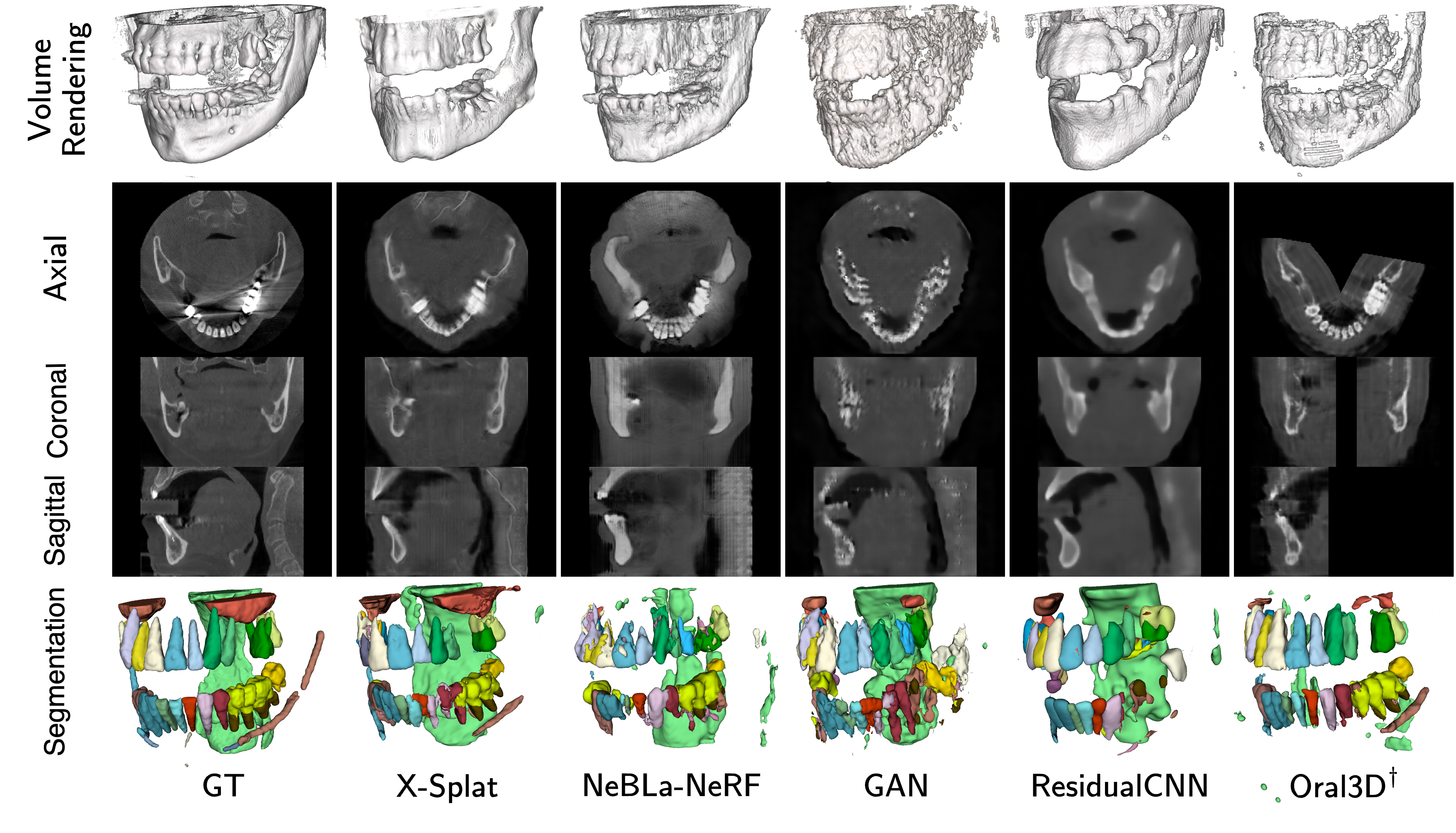
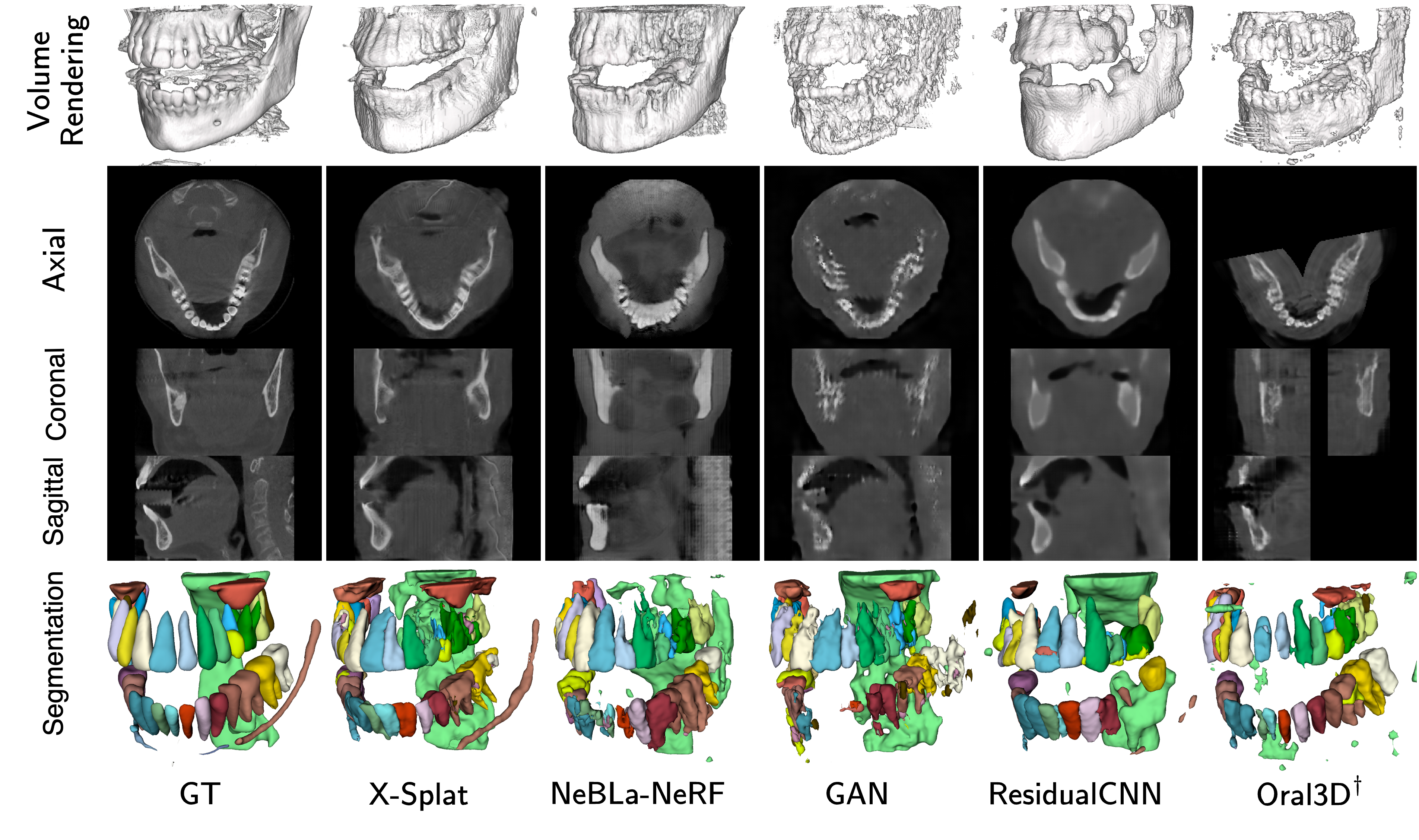
Qualitative results. Figure 4 shows generations for a representative case. X-Splat recovers the full craniofacial anatomy of the ground-truth CBCT: cortical and trabecular bone are clearly
separated, the maxillary sinuses form well-defined hypodense cavities, and the inferior alveolar nerve canal appears as a continuous tubular structure through the mandible. The anisotropic Gaussians drive the sharp cortical boundaries, rendering the dense
mineralized jaw shell as a bright high-attenuation rim in axial and coronal sections, which demands the precise ray-boundary localization that isotropic or implicit representations lack. Figure 3 visualizes the
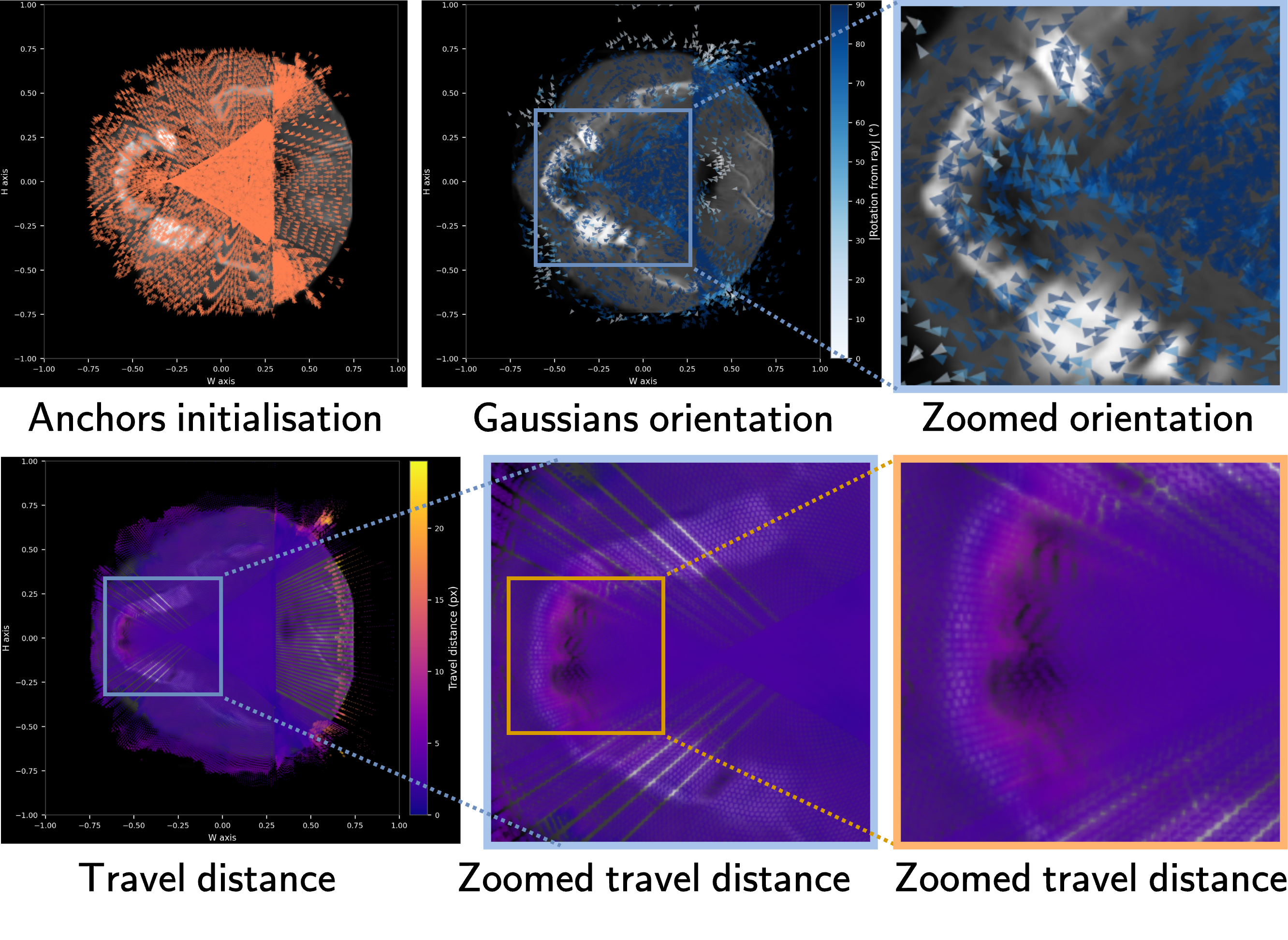
learned orientation and displacement of Gaussian primitives, confirming that splats actively rotate to align with anatomical boundaries and migrate toward high-density tissue regions during inference.
Competing methods recover coarser anatomy with less detail. NeBLa partially reconstructs bone but blurs the trabecular–cortical interface and misses the sinuses. Residual CNN is diffuse and over-smoothed with weak cortical definition, while the GAN
introduces spurious high-frequency artifacts from optimising the maximum-intensity-projection loss. Oral-3D reconstructs only the dental-arch sub-volume, omitting the surrounding bony and soft-tissue anatomy (e.g.pharynx and spine).
The segmentation row highlights a key advantage: predicted tooth labels appear only where teeth exist in the ground truth, showing that X-Splat does not hallucinate dental structures in edentulous regions, a consequence of multi-view DRR regularization
penalizing any density unsupported by projections from multiple directions.
Ablation study. Table 1 isolates the contribution of each component; extended ablation in Appendix 6.5. Densifying NeBLa’s default ray count from 256 to 320 yields only
marginal TVR gains, leaves BA-ASD unchanged (\(35.67\) vs.\(35.66\) mm), and doubles hallucinated volume, showing that the NeRF implicit field, not ray density, is the bottleneck.
Replacing this field with fixed Gaussian anchors and no refiner alone cuts BA-ASD by \(2.9\times\) (\(35.67\!\to\!12.45\) mm) and raises PSNR to \(22.97\) dB, confirming ray-anchored anisotropic Gaussians are a far better representation for this task. Allowing ray-aligned Gaussian movement further improves TVR and lowers hallucinated volume from \(3.49\%\) to \(2.45\%\), so migration toward anatomy acts as an implicit geometric regularizer.
The refiner is only beneficial under geometric supervision. Added alone, it degrades BA-ASD from \(12.98\) to \(22.91\) mm and increases hallucinations, shifting the generation burden from
the Gaussian stage to learned priors. Adding \(\mathcal{L}_\mathrm{mv}\) gives the single largest gain in the ablation, restoring BA-ASD to \(2.39\) mm (\(9.6\times\)) while suppressing hallucinations, confirming that multi-view better resolves depth ambiguity and constrains the refiner.
The full model attains the best BA-ASD, SSIM, and LPIPS. Its TVR (\(84.96\%\)) is not the highest in isolation, variant #2 reaches \(88.16\%\), but at the cost of BA-ASD (\(12.98\) mm), exposing a recall–geometry trade-off. Overall, each component addresses a distinct failure mode: Gaussians provide geometric precision, movement adds expressivity and regularization, multi-view supervision enforces
depth consistency, and coarse supervision anchors geometric fidelity in the Gaussian stage before refinement.
4 Conclusions↩︎
We present X-Splat, a feed-forward Gaussian Splatting framework for generating CBCT-like 3D maxillofacial volumes from a single panoramic radiograph, treating the known acquisition geometry as a generation scaffold: anisotropic Gaussian primitives anchored to the X-ray paths are displaced, rotated, and scaled to recover 3D anatomical structure. Coupled with Beer–Lambert reprojection, multi-view DRR supervision, and a lightweight residual refiner, this converts an otherwise highly underdetermined problem into a geometry-constrained volumetric inference task.
X-Splat improves over NeRF- and GAN-based baselines in big anatomy surface accuracy, mandibular canal recovery, and hallucination suppression, suggesting that explicit Gaussian representations are well suited to dental generation, where thin cortices,
root boundaries, and canal structures require localized geometric control rather than unconstrained volumetric generation.
This work is a step toward 3D dental generation from routine panoramic imaging. While our results are consistent across both quantitative metrics and qualitative evidence, the cohort is limited to scans with full maxillofacial field of view and paired
segmentation labels. Generalization to more diverse patient populations and imaging conditions remains to be established. Our study uses CBCT-derived simulated panoramics, which provide paired supervision and controlled evaluation but do not fully capture
the variability of real panoramic systems; future work will focus on multi-site training, real-PXR adaptation, and tissue-specialized Gaussian densification. By showing that ray-anchored Gaussian primitives can recover detailed maxillofacial structure from
a single projection, X-Splat opens a path toward scalable 3D dental analysis in settings where CBCT is unavailable, impractical, or unnecessary.
5 Related Work↩︎
5.1 3D generation from Panoramic Radiographs↩︎
Recovering 3D oral anatomy from a panoramic radiograph has progressed from GAN-based volumetric prediction toward physics-aware implicit representations. We organize prior work by generation scope (individual teeth vs.the complete oral volume) and by physics grounding.
Tooth-level generation. A first line recovers individual tooth shapes as meshes, point clouds, or occupancy fields rather than full CBCT intensities. X2Teeth [13] was the first CNN framework to reconstruct the occupancy of all teeth from a single PXR via localization and patch-wise generation sub-networks. Occudent [14] used neural implicit occupancy from shape and class embeddings, PX2Tooth [15] extended this to point clouds with a root-apex prior, and DTR-Net [38] jointly reconstructed intensities and tooth geometry in a dual space. However, all reconstruct only tooth geometry, omitting alveolar bone, the mandibular canal, the maxillary sinus, and soft tissue, and thus cannot serve as standalone tools for implant or surgical planning.
Volumetric oral generation. A second line recovers tooth and bony anatomy as intensity volumes. Oral-3D [10] was the first to generate a 3D oral volume from a single PXR with a GAN [18], but requires the dental arch curve as input, not available at inference, and resolves only a rectified box around it, excluding surrounding anatomy such as the spine. It further limits generation to dense tissues such as bone and teeth, omitting soft-tissue structures including the pharynx, maxillary sinuses, and the mandibular canal. 3DPX [12] improved depth inference with a hybrid MLP-CNN pyramid. Neither imposes a physics-consistent constraint linking the volume to the observed projection, nor regularizes against anatomical structure, leaving the output dependent on the learned mapping’s generalization.
Physics-grounded generation. NeBLa [11] is the most physically principled single-view method, synthesizing a synthetic PXR intermediate via the Beer–Lambert law and a ray-tracing neural model, with real PXR translated to synthetic style at inference. While this bridges the synthetic-to-real gap, the core generation remains limited. NeBLa voxelizes implicit NeRF densities into a coarse volume and passes it to a large volumetric refiner, applying supervision only to the final refined output. Without geometric constraints on the coarse volume, depth ambiguity may remain unresolved where it matters most, and the large refiner may favor memorization of population-level anatomy over recovery of input-consistent geometry. The implicit representation further risks losing sharp root boundaries and canal cortex by construction, and imposes no geometrical prior, so globally inconsistent hallucinations may arise.
5.2 Sparse-View Neural Volumetric Generation↩︎
A broader body of work reconstructs volumes from sparse X-ray projections, providing the representations and physical rendering models relevant here.
NeRF-based CT. Adapting NeRF to X-ray replaces surface-reflectance rendering with the Beer–Lambert attenuation integral. IntraTomo [9] introduced a self-supervised formulation, NeAT [39] added octree-based empty-space culling, and NAF [7] specialized CBCT with hash encodings on jaw data via TIGRE [40]. SAX-NeRF [41] added the Lineformer architecture and the X3D dataset, while geometry-aware attenuation learning [8] and its vessel-guided extension [42] back-project multi-view features for high-quality generation from 5–10 views. In all cases, multi-view projections remain a prerequisite for resolving the volume.
Gaussian Splatting for X-ray and CT. X-Gaussian [23] first applied 3DGS to X-ray with differentiable radiative rasterization and SfM-free initialization. \(R^2\)-Gaussian [24] corrected an integration bias in X-ray 3DGS and added a differentiable voxelizer, 3DGR-CT [43] used FBP-guided initialization, and FaCT-GS [44] showed GS benefits are largest in the sparse-view regime. Separately, anatomy-aware supervision improves clinical quality beyond pixel-wise losses: CARE [21] shows PSNR/SSIM are largely insensitive to small critical structures and adds segmentation-guided completeness penalties, but operates in a self-supervised, scene-level setting driven by multi-view reprojection and acts as a post-hoc plug-in. Together, these works establish physics-consistent GS as a competitive paradigm for sparse-view CT, offering explicit geometry, fast convergence, and direct volume extraction; yet they rely on multi-view spatial redundancy and lack dataset-level priors, so they cannot resolve the null-space of a single projection.
Single-view generation. Unlike per-subject sparse-view optimization, single-view generation is an ill-posed one-to-many mapping requiring strong statistical priors, motivating supervised learning on paired PXR–CBCT data. In natural images, this has been addressed by GANs [18], encoder–decoders [31], multi-view architectures [30], and cross-modal synthesis [17], and more recently by large learned priors such as Wonder3D [45], LRM [46], and InstantMesh [47]. The shared insight is that a prior learned from large-scale data resolves the ambiguity a single view leaves open; for X-ray, however, that prior must capture anatomical structure and geometry rather than image-space appearance.
In summary, prior PXR-to-3D methods either recover isolated tooth geometry or full volumes without physics-consistent rendering or geometric regularization; sparse-view CT methods provide the rendering tools but require multiple projections, and their supervision has been limited to scene-level settings. Combining physics-consistent Gaussian Splatting with geometry-driven supervision in the dataset-level, single-view PXR-to-CBCT regime remains open, and is the core contribution of this work.
6 Experimental setup↩︎
6.1 Dataset↩︎
ToothFairy3. We use data from ToothFairy3 [35]–[37], a publicly available CBCT dataset released in conjunction with the ToothFairy3 MICCAI-ODIN 2025 challenge [35]. The dataset comprises three acquisition subsets that differ in scanner and field-of-view (FoV): Set A (417 volumes) and Set C (52 volumes), both restricted to the mandibular region or limited in FoV with partially cropped maxilla, acquired to capture the inferior alveolar nerve canal; and Set B (63 volumes), acquired with a broader FoV covering the complete maxillofacial anatomy, including all upper and lower teeth from crown to root apex, the maxillary sinuses, pharynx, and surrounding bony structures. Segmentation labels follow an extended FDI World Dental Federation notation covering 77 classes: jawbones, inferior alveolar and incisive canals, maxillary sinuses, pharynx, prosthetics (bridges, crowns, implants), 32 individual teeth, and the corresponding pulp chambers (32).
Subset selection. Single-PXR-to-CBCT reconstruction requires a full maxillofacial field of view, as the panoramic projection integrates anatomy from both arches and surrounding structures. We therefore restrict training and evaluation to Set B and further apply two quality criteria: (i) no more than 50% missing dentition, ensuring sufficient tooth anatomy for meaningful geometric evaluation, and (ii) complete crown-to-apex visibility for all present teeth with no dental structures cropped at the volume boundary. Applying these criteria to the 63 Set B volumes yielded 60 eligible scans with paired segmentation labels. These were randomly partitioned into training (\(n{=}45\)), validation (\(n{=}5\)), and test (\(n{=}10\)) sets, with the proportion of partially edentulous patients kept comparable across all three splits.
6.1.1 Segmentation Model for Geometry-Aware Evaluation↩︎
To evaluate the geometric fidelity of generated volumes we use an automated segmentation model as a structure-level evaluator: the model is applied independently to each predicted volume and to the corresponding ground-truth CBCT, and the resulting label maps are compared to compute the geometry-aware metrics (BA-ASD, TVR, CVR, HV) and explained in more details is Appendix 6.4.
We use recent method GEPAR3D [28], [29] which excels in CBCT segmentation generalization [48], a feed-forward segmentation network that unifies instance-level detection and multi-class segmentation in a single pass, adapted here to the full ToothFairy3 label space. The model was trained on full-maxillofacial FoV CBCT scans, the only subset of ToothFairy3 containing complete upper and lower arch annotations and validated on the subsets (Set A and Set C), which despite their restricted field of view provide independent anatomical coverage for the lower arch, canals, and jawbone.
As an evaluator, GEPAR3D is applied uniformly to all methods and to ground truth; any segmentation inaccuracies it introduces therefore affect all predictions consistently, preserving the validity of relative comparisons. Crucially, any missed structures produce pessimistic metric estimates: a tooth or canal volume that the evaluator fails to detect lowers TVR and CVR scores for every method equally, so reported geometry-aware improvements constitute lower bounds on true structural recovery. This conservative behaviour is particularly relevant for fine structures such as root apices, where segmentation uncertainty is highest and reported scores may underestimate true recovery.
6.2 Implementation Details↩︎
6.2.1 Network Architecture↩︎
6.2.1.1 2D U-Net encoder.
The panoramic image \(\mathbf{I}\) is processed by a 2D U-Net that produces a dense feature map \(\mathbf{F}\in\mathbb{R}^{H_p\times W_p\times 128}\) at the input resolution. All convolutional blocks use the double-convolution design (two \(3\!\times\!3\) convolutions per block), max-pool downsampling, bilinear upsampling, and instance normalization. Features at a given pixel location are read directly at the index corresponding to each Gaussian anchor’s ray-pixel mapping.
6.2.1.2 Shared MLP.
A single eight-layer MLP \(f_\phi\) of width 128 is shared across all \(N_g\) anchors. For anchor \(j\), the encoder feature \(\mathbf{F}(\mathbf{p}_j)\) and the sinusoidal positional encoding \(\mathrm{PE}(\mathbf{p}_j)\) with \(L=7\) frequency bands are each passed through a learned linear projection and summed to form an initial fused representation \(\mathbf{h}_0\), queried at a single pixel following [11], [16]. Eight subsequent layers with ReLU activations process \(\mathbf{h}_0\); a skip connection at the network midpoint concatenates \(\mathbf{h}_0\) back into the hidden state before the second half of the network, following the NeRF residual conditioning scheme [16]. \(f_\phi\) outputs the raw displacement scalar \(\hat{\delta t}_j\), log-scale vector \(\mathbf{s}_j\in\mathbb{R}^3\), unit quaternion \(\mathbf{q}_j\in\mathbb{R}^4\), and scalar density \(\alpha_j\).
6.2.1.3 Gaussian representation.
A total of \(N_g = 6{,}553{,}600\) anisotropic 3D Gaussians are anchored along panoramic acquisition rays (\(128\text{ slices}\times256\text{ rays}\times 200\text{ samples}\), matching the ray-sample count of the SimPX renderer). All three scale axes are initialized uniformly to \(\sigma_0=0.25\;\text{px}\) and clamped throughout training to \([0.25,\,1.0]\;\text{px}\). Movement is restricted to the 1-D displacement \(\delta t_j = \tanh(\hat{\delta t}_j)\cdot\delta t_{\max}\) along the anchor ray within the axial (\(XY\)) plane, with \(\delta t_{\max}=32\) voxels; the \(Z\)-component is held at zero to preserve the dense axial coverage. Rotation is restricted to the axial plane (rotation around the \(Z\)-axis only). Density is activated with a softplus function, and Gaussian rasterization uses the differentiable R2-Gaussian CUDA voxelizer [24].
6.2.1.4 3D residual refiner.
The refiner \(r_\psi\) is a compact 3D U-Net with three encoder/decoder stages and feature widths \([32, 64, 128]\), parameterized as a residual correction \(\hat{V}_f = \hat{V}_c + r_\psi(\hat{V}_c)\). All convolutional blocks follow the double-convolution design with strided-convolution downsampling, trilinear upsampling, and instance normalization. The final \(3\!\times\!3\!\times\!3\) convolutional layer is zero-initialized so that \(r_\psi(\hat{V}_c)=\mathbf{0}\) at the start of training, ensuring that early gradient signal flows through the Gaussian parameters and MLP before the refiner contributes.
A full summary of architectural hyperparameters is given in Table 2.
| Hyperparameter | Value |
|---|---|
| 2D U-Net encoder | |
| Output feature channels | 128 |
| Convolution blocks | double (\(3\times3\)) |
| Downsampling | max-pool |
| Upsampling | bilinear |
| Normalization | instance |
| Shared MLP | |
| Depth (layers) | 8 |
| Width (channels) | 128 |
| Positional encoding frequencies \(L\) | 7 |
| Feature query radius | single pixel |
| Gaussian representation | |
| Total anchors \(N_g\) | 6,553,600 |
| Scale type | anisotropic (3 axes) |
| Scale initialization \(\sigma_0\) | 0.25 px |
| Scale clamp range | \([0.25,\;1.0]\) px |
| Movement mode | 1-D along ray (\(XY\)) |
| Max displacement \(\delta t_{\max}\) | 32 vox |
| Rotation mode | axial (\(Z\)-axis only) |
| Density activation | softplus |
| Voxelizer | R2-Gaussian [24] |
| 3D residual refiner | |
| Stages | 3 |
| Feature widths | \([32,\;64,\;128]\) |
| Convolution blocks | double (\(3\times3\times3\)) |
| Downsampling | strided convolution |
| Upsampling | trilinear |
| Normalization | instance |
| Final convolution kernel | \(3\times3\times3\) |
| Final convolution initialization | zero |
| Volume | |
| Output shape \((X\!\times\!Y\!\times\!Z)\) | \(256\times256\times128\) |
6.2.2 SimPX Ray Geometry and Rendering↩︎
We adopt the SimPX focal-trough geometry from NeBLa [11] without modification. Table 3 lists all rendering constants. The \(K=200\) uniformly spaced samples per ray define the anchor grid together with the \(128\times256\) panoramic image dimensions, yielding \(N_g=6{,}553{,}600\) anchor positions. The Beer-Lambert rendering constants (\(I_0\), \(\beta\), \(p_{\max}\)) are inherited from the NeBLa calibration and held fixed throughout training. Synthetic PXR–CBCT pairs are registered at no acquisition cost. Matched real pairs are clinically rare, and verifying sub-voxel registration between them is non-trivial. Synthetic training scales to any CBCT dataset and provides exact ground-truth supervision under a physically calibrated forward model.
| Parameter | Value |
|---|---|
| Coordinate system | LPS |
| Rotation centres \(n_c\) | 21 |
| Samples per ray \(K\) | 200 |
| Ray-length multiplier | 0.5 |
| Angular step (molar) | 0.528 rad |
| Angular step (default) | 0.600 rad |
| Angular step (front) | 1.509 rad |
| Attenuation step \(\Delta s\) (ray_delta) | 1.35 |
| Render sample mode | nearest-neighbour |
| \(I_0\) | 1.0 |
| \(\beta\) | \(7.5\times10^{-7}\) |
| \(p_{\max}\) | 0.25 |
| HU scaling method | direct scaling |
6.3 Training Details↩︎
6.3.0.1 Dataset and preprocessing.
We use a subset of the publicly available ToothFairy3 dataset [35]–[37], retaining scans with no more than 50% missing dentition and a full maxillofacial field of view, where every visible tooth is fully captured from crown to root apex without cropping. Applying these criteria yielded 60 eligible CBCT volumes with paired segmentation labels, partitioned into training (\(n{=}45\)), validation (\(n{=}5\)), and test (\(n{=}10\)) sets while maintaining a comparable proportion of partially edentulous patients across all splits.
All volumes are resampled isotropically from their native resolution of \(0.3\;\text{mm\,px}^{-1}\) to \(0.65\;\text{mm\,px}^{-1}\), yielding a canonical grid of \(256\!\times\!256\!\times\!128\) voxels that covers the full maxillofacial field of view within GPU memory. Intensity volumes are resampled with trilinear interpolation. Segmentation label maps are resampled via one-hot interpolation: each class is first binarized into a separate channel, the resulting stack of binary maps is interpolated linearly, and the final label is recovered by \(\operatorname{argmax}\) across channels. Compared to nearest-neighbor resampling, this preserves the boundaries of thin structures (root apices, mandibular canal) that could otherwise be corrupted by the coarser target grid.
X-Splat is trained exclusively on synthetic Synthetic PXR–CBCT pairs: panoramic projections are synthesized from each ground-truth CBCT using the Beer-Lambert renderer and the scanning geometry, yielding perfectly registered input–output pairs at no
acquisition cost. SimPXRs intensities are normalized by a single global physics constant \(p_{\max}=0.25\), the divisor already embedded in the Beer-Lambert renderer, with the zero lower bound (background air) left
unchanged. Unlike per-image or per-dataset-range rescaling, dividing by a fixed constant preserves the physics-consistent correspondence between CBCT HU values and Synthetic PXR pixel intensities: the same tissue density must map to the same projected
attenuation regardless of the patient, which any data-driven normalization would destroy. The value \(p_{\max}=0.25\) is physically grounded: with the calibrated Beer-Lambert parameter \(\beta=7.5\!\times\!10^{-7}\) and \(K=200\) ray samples, the integrated log-attenuation across the full dental anatomy does not exceed \(p_{\max}\) in any scan in
the dataset, so no clipping of Synthetic PXR values occurs. CBCT intensities are clipped to \([\mathrm{HU}_{\min},\mathrm{HU}_{\max}]
=[0,\,4000]\) (spanning air through dense enamel) and rescaled linearly to \([0,\,1]\). The full dataset is pre-cached in memory at the start of training (cache_rate = 1.0).
6.3.0.2 Multi-view DRR supervision.
During training \(N=31\) azimuthal DRR projections are rendered at \(\Delta\theta=7.5^{\circ}\) spacing over \(\pm112.5^{\circ}\) (\(225^{\circ}\) total arc, including the \(0^{\circ}\) centre view). Perceptual supervision is applied to the fine volume \(\hat{V}_f\) at the eight symmetric angles \(\theta\in\{{\pm}37.5^{\circ},{\pm}52.5^{\circ},{\pm}67.5^{\circ},{\pm}82.5^{\circ}\}\) (DRR indices 4, 6, 8, 12, 18, 22, 24, 26 in the ordered stack).
6.3.0.3 Loss weights.
All losses are computed independently for the coarse volume \(\hat{V}_c\) and the refined volume \(\hat{V}_f\) and summed. Perceptual losses are applied to \(\hat{V}_f\) only. Table 4 lists all weights; note that MIP-axis weights are uniform (\(x:y:z=1:1:1\)).
| Loss | Symbol | Fine \(\hat{V}_f\) | Coarse \(\hat{V}_c\) |
|---|---|---|---|
| Volumetric MSE | \(\lambda_{\mathrm{rec}}\) | 10 | 5 |
| Beer-Lambert reprojection | \(\lambda_{\mathrm{proj}}\) | 50 | 50 |
| MIP projection (3 axes) | \(\lambda_{\mathrm{mip}}\) | 10 | 5 |
| Multi-view DRR | \(\lambda_{\mathrm{mv}}\) | 150 | 50 |
| Perceptual (Beer-Lambert) | \(\lambda_{\mathrm{perc,proj}}\) | 0.05 | — |
| Perceptual (MIP) | \(\lambda_{\mathrm{perc,mip}}\) | 0.01 | — |
| Perceptual (multi-view DRR) | \(\lambda_{\mathrm{perc,mv}}\) | 0.02 | — |
5pt
Weights were calibrated once on a held-out validation case after training had stabilized at approximately 100 epochs and were then fixed for all reported experiments.
6.3.0.4 Optimizer and learning-rate schedule.
All parameters are trained with AdamW. Per-parameter-group overrides are used to account for the distinct roles of encoder, MLP, and refiner (Table 5); parameters not assigned to a named group fall back to the global settings.The MLP receives a modestly elevated learning rate [24], reflecting its primary responsibility for solving the 3D geometric lifting problem from the 2D conditioning signal. A cosine annealing schedule reduces every group’s learning rate from its initial value to \(\eta_{\min}=10^{-5}\) over 500 epochs with no restarts.
| Parameter group | Learning rate | Weight decay |
|---|---|---|
| Global (default) | \(1\times10^{-3}\) | \(1\times10^{-6}\) |
| Encoder | \(1\times10^{-3}\) | \(1\times10^{-4}\) |
| MLP | \(1.2\times10^{-3}\) | \(1\times10^{-6}\) |
| Refiner | \(1\times10^{-3}\) | \(1\times10^{-4}\) |
| Scheduler | cosine, \(\eta_{\min}=10^{-5}\) | |
6.3.0.5 Training schedule and initialization.
Models are trained for 500 epochs with batch size 1 and random seed 42. The residual refiner is active from epoch 0. X-Splat is warm-started from a prior checkpoint that does not include the refiner; on loading, any mismatched or absent parameter keys are discarded and newly added parameters (refiner weights) are initialized from scratch. The best checkpoint is selected based on loss value, which consists of raw unscaled value of projection (MIP) and MSE 3D losses.
6.3.0.6 Hardware and software.
All experiments are run on a single NVIDIA GPU A100 80GB with PyTorch mixed precision in bfloat16. cuDNN benchmark mode is enabled. The R2-Gaussian voxelizer is compiled as a custom CUDA extension. No gradient clipping is applied.
6.4 Evaluation metrics↩︎
| Overlap-based | Geometry-aware | |||||
|---|---|---|---|---|---|---|
| 2-3(l)4-7 Method | Thr. DSC \(\uparrow\) | Seg. DSC \(\uparrow\) | BA-ASD \(\downarrow\) | TVR \(\uparrow\) | CVR \(\uparrow\) | HV \(\downarrow\) |
| X2CT-GAN [17] | \(16.11_{13.22}\) | \(18.57_{7.77}\) | \(58.60_{15.98}\) | \(25.95_{23.86}\) | \(1.88_{2.26}\) | \(4.38_{8.00}\) |
| R2N2 [30] | \(33.12_{7.64}\) | \(34.57_{10.61}\) | \(28.98_{19.01}\) | \(36.08_{7.64}\) | \(0.01_{0.02}\) | \(19.27_{16.46}\) |
| Residual CNN [31] | \(38.78_{9.16}\) | \(41.09_{13.24}\) | \(13.06_{12.29}\) | \(66.80_{9.58}\) | \(\underline{27.62_{21.28}}\) | \(14.95_{18.25}\) |
| GAN [32] | \(43.08_{5.89}\) | \(\underline{44.90_{6.75}}\) | \(\underline{10.60_{16.59}}\) | \(70.29_{10.50}\) | \(9.11_{7.70}\) | \(14.36_{15.04}\) |
| NeBLa [11] | \(\underline{43.41_{7.26}}\) | \(36.08_{11.71}\) | \(35.67_{21.97}\) | \(\underline{74.12_{3.64}}\) | \(1.14_{1.27}\) | \(\underline{3.99_{5.33}}\) |
| 1-1(l)2-3(l)4-7 Oral-3D [10] | \(66.61_{5.89}\)\(^{\dagger\ddagger}\) | \(38.54_{8.96}\)\(^{\dagger\ddagger}\) | \(47.55_{18.27}\)\(^\ddagger\) | \(76.58_{10.79}\)\(^\ddagger\) | \(48.35_{22.73}\)\(^\ddagger\) | \(1.07_{1.47}\)\(^\ddagger\) |
| X-Splat (Ours) | \(\mathbf{45.76_{8.59}}\) | \(\mathbf{53.68_{11.39}}\) | \(\mathbf{2.39_{0.74}}\) | \(\mathbf{84.96_{4.51}}\) | \(\mathbf{67.33_{19.83}}\) | \(\mathbf{2.96_{5.16}}\) |
Prior reconstruction methods [10], [11] evaluate volumetric overlap using an intensity threshold to binarize predictions, a reasonable proxy when segmentation labels are unavailable. However, this approach carries two limitations that are particularly pronounced in single-view CBCT generation. First, the threshold must be chosen to separate tissue from background in predictions whose intensity distributions vary across methods, introducing a systematic bias that favors methods whose output statistics happen to align with the chosen value. Second, depth along the projection axis is inherently ambiguous in single-view reconstruction, so a geometrically plausible prediction that recovers all anatomical structures at a slightly shifted position is penalized as severely as one that misses them entirely. Critically, a model that generates anatomy close to the population mean will score highly on threshold DSC regardless of whether it reflects the input radiograph, rewarding hallucination of average anatomy over patient-specific reconstruction. The availability of dense segmentation labels in ToothFairy3 enables us to move beyond this proxy. We therefore prioritize surface-distance metrics expressed in millimeters, which assess geometric fidelity directly in physical space and are largely immune to this ambiguity, alongside volume-recall and hallucination measures that capture clinically relevant completeness and specificity.
Big Anatomy ASD (BA-ASD, mm \(\downarrow\)) reports the symmetric Average Surface Distance over the five major craniofacial structures \(\mathcal{K}\) (mandible, maxilla,
bilateral maxillary sinuses, pharynx) [27]: \[\begin{align}
\text{BA-ASD} = \frac{1}{|\mathcal{K}|}\sum_{k \in \mathcal{K}} \frac{1}{2}\Bigl( &\frac{1}{|S_k|}\sum_{p \in S_k} \min_{q \in \hat{S}_k} \|p-q\|_2 \\ +\,&\frac{1}{|\hat{S}_k|}\sum_{q \in \hat{S}_k} \min_{p \in S_k} \|p-q\|_2 \Bigr),
\end{align}\] where \(S_k\) and \(\hat{S}_k\) are the ground-truth and predicted surfaces of structure \(k\). When a structure is absent from the
prediction, a finite penalty equal to half the volume diagonal is assigned following [27], ensuring all cases contribute a comparable value
without requiring a binary presence threshold. Teeth Volume Recall (TVR, % \(\uparrow\)) measures, for each tooth class present in the ground truth, the fraction of its expected tissue volume reconstructed
by the model, averaged over all present classes; a model that reconstructs only a subset of teeth scores accordingly low, preventing partial reconstructors from appearing competitive. Canal Volume Recall (CVR, % \(\uparrow\)) applies the same measure to the inferior alveolar nerve canal (mandibular nerve canal), a thin tubular structure that is clinically critical yet difficult to recover. Hallucinated Volume (HV,
% \(\downarrow\)) measures the total volume of falsely predicted tooth structures for tooth classes absent from the ground truth, expressed as a fraction of the ground-truth teeth volume, directly quantifying the tendency
to fabricate anatomy. Intensity-based metrics (PSNR \(\uparrow\), SSIM \(\uparrow\), LPIPS \(\downarrow\)) are retained as global fidelity measures and to
enable direct comparison with prior work that does not report geometry-aware evaluation.
While Section 6.4 argues that overlap-based metrics are unreliable discriminators of reconstruction quality in this task, we report them here for completeness and to enable direct comparison with prior
work [10], [11] that reported this criterion.
Table ¿tbl:tab:supp95dice? reports threshold and segmentation Dice Scores alongside the geometry-aware metrics. Thr. DSC is computed at \(0.4\) (\({\approx}600\) HU on the
normalized \([-1000,3000]\) HU scale), which lies above soft tissue and evaluates dense mineralized structures only, excluding the mandibular canal, pharynx, and sinuses that X-Splat explicitly reconstructs. Seg. DSC is
computed against binarized ground-truth big anatomy segmentation labels, directly measuring whether predicted tissue coincides with actual anatomy rather than any high-attenuation region. X-Splat achieves the best score on both metrics among
oracle-free full-volume methods (\(45.76\) and \(53.68\) respectively), and is the only method for which Seg. DSC exceeds Thr. DSC, an increase of \(7.92\)
points indicating that its predictions concentrate high-attenuation tissue in anatomically consistent area. The contrasting behavior of NeBLa is instructive: its Thr. DSC of \(43.41\) is competitive, but Seg. DSC drops to
\(36.08\), a fall of \(7.33\) points. This reversal indicates that NeBLa generates plausible high-attenuation intensities whose spatial distribution may approximate the population mean
rather than the specific patient, aligning well with a fixed threshold but poorly with actual labels. The insensitivity of Thr. DSC to geometric accuracy is further illustrated by Residual CNN and NeBLa: Residual CNN achieves a \(2.7\times\) lower BA-ASD than NeBLa (\(13.06\) vs.\(35.67\) mm), indicating substantially more accurate anatomical placement, yet scores \(4.63\) points lower on Thr. DSC (\(38.78\) vs.\(43.41\)), demonstrating that a method generating geometrically correct anatomy at a slightly shifted
position is penalized more than one producing mean-anatomy at the right average location. Oral-3D exhibits the same pattern despite oracle arch geometry and evaluation restricted to the arch sub-volume: Thr. DSC of \(66.61\) collapses to \(38.54\) on Seg. DSC, suggesting that even within its privileged reconstruction region, predicted tissue does not reliably coincide with ground-truth dental anatomy. The
divergence between Thr. DSC and Seg. DSC across methods confirms that a fixed intensity threshold is questionably reliable proxy for geometrical and anatomical accuracy in this task.
Comparison with state-of-the-art. We evaluate X-Splat against six representative single-view 3D generation methods. NeBLa [11] is the current state-of-the-art for CBCT generation from a single panoramic radiograph, combining the Beer-Lambert driven panoramic ray geometry with a NeRF-style
implicit field supervision; X-Splat builds directly upon its ray geometry and projection model. Oral-3D [10] is a GAN-based method
that reconstructs 3D oral structures from a single panoramic image by learning a flattened volumetric representation that is then geometrically deformed and interpolated back into 3D space using the dental arch curve as a spatial deformation operator. In
our implementation the arch is derived from ground-truth tooth label centroids and jaw bone skeleton, constituting oracle geometric access normally not available at inference time. R2N2 [30] reconstructs 3D shapes from images via a recurrent encoder; following [11], the
recurrent connection is removed for the single-image setting. Residual CNN [31] employs an encoder-decoder network for
volumetric generation. GAN [32] uses the Residual CNN as generator paired with an adversarial
discriminator. X2CT-GAN [17] reconstructs CT volumes from biplanar X-rays, adapted here to the single-view setting. Prior
panoramic generation methods, including NeBLa and Oral-3D, focus primarily on hard dental tissues such as teeth and jaw bone. We train and evaluate all methods on the full maxillofacial volume, including soft-tissue cavities and the mandibular canal,
providing a more complete assessment of generation quality.
| \(N\) | \(\delta t_{max}\) | Intensity-based | Geometry-aware | ||||
|---|---|---|---|---|---|---|---|
| 3-5(lr)6-8 | PSNR \(\uparrow\) | SSIM \(\uparrow\) | LPIPS \(\downarrow\) | BA-ASD \(\downarrow\) | TVR \(\uparrow\) | HV \(\downarrow\) | |
| 1.5M | 32 | \(23.16_{0.67}\) | \(78.16_{0.98}\) | \(0.291_{0.006}\) | \(12.63_{16.93}\) | \(87.90_{4.10}\) | \(3.69_{5.70}\) |
| 3M | 32 | \(23.24_{0.72}\) | \(79.86_{1.09}\) | \(0.268_{0.007}\) | \(5.15_{9.24}\) | \(88.66_{5.37}\) | \(3.86_{4.38}\) |
| 6M | 32 | \(23.27_{0.91}\) | \(79.62_{1.76}\) | \(0.259_{0.015}\) | \(2.39_{0.74}\) | \(84.96_{4.51}\) | \(2.96_{5.16}\) |
| 3M | 32 | \(23.24_{0.72}\) | \(79.86_{1.09}\) | \(0.268_{0.007}\) | \(5.15_{9.24}\) | \(88.66_{5.37}\) | \(3.86_{4.38}\) |
| 3M | 48 | \(23.05_{0.70}\) | \(78.61_{1.07}\) | \(0.265_{0.006}\) | \(6.98_{14.73}\) | \(88.07_{4.04}\) | \(2.78_{3.11}\) |
| 3M | 64 | \(23.17_{0.70}\) | \(78.21_{1.06}\) | \(0.281_{0.006}\) | \(4.66_{7.36}\) | \(87.99_{3.54}\) | \(2.81_{4.70}\) |
4pt
6.5 Ablation study↩︎
Table 6 ablates Gaussian count and travel budget. Increasing \(N\) from 1.5M to 3M produces the sharpest geometry gain in this experiment: BA-ASD falls from \(12.63\) to \(5.15\) mm, indicating that at 1.5M inter-anchor gaps are wide enough that splats cannot fill the density field without approaching the scale limit, leaving regions either absent or
covered by splats whose anchor features do not correspond to that location. A further doubling to 6M halves BA-ASD again (\(5.15\!\to\!2.39\) mm) while SSIM slightly decreases (\(79.86\!\to\!79.62\%\)), showing that geometry-aware metrics remain sensitive to splat density beyond the point at which intensity metrics saturate. We therefore select \(N\)=6M for the proposed
model; the 3M configuration is a practical alternative under compute constraints, recovering most intensity quality at half the primitive count. This efficiency is unavailable to implicit NeRF representations, whose sample count is fixed by the ray
grid and cannot be spatially concentrated on anatomy.
For travel distance, \(\delta t_{\max}\)=32 gives the best overall balance. As we showed, most Gaussians use only a small fraction of the permitted range (Gaussian Dynamic Figure), with productive migrations concentrated as
short-range adjustments toward tissue boundaries; the budget therefore acts as a regulariser rather than an active constraint. Larger values modestly reduce hallucinated volume (HV \(3.86\!\to\!2.78\) at \(\delta t_{\max}\)=48) but degrade both SSIM and TVR. Since actual displacement remains well below the budget, a larger \(\delta t_{\max}\) compresses the used portion of the tanh output into a
steeper region of the curve, increasing gradient sensitivity and likely destabilizing optimisation without expanding the range productively used in practice.
Scale range was not ablated independently: it is determined by the panoramic ray geometry and constitutes a design constraint rather than a tunable hyperparameter. Splats are initialized at \(1\sigma\)=0.25 px and allowed
to grow up to a maximum whose \(3\sigma\) extent does not significantly overlap the nearest neighboring ray, directly preserving the per-ray PXR conditioning that underlies the method. Relaxing this bound to compensate for
sparser coverage at lower \(N\) would cause splats to extend across multiple rays, so that each Gaussian’s density is no longer informed exclusively by its anchor ray feature, thus invalidating the core conditioning
mechanism rather than ablating \(N\) in isolation. At \(N\)=1.5M, some inter-ray gaps cannot be filled without splats exceeding the scale bound. Along-ray displacement can reposition splats
within their ray but cannot place density between rays, leaving those regions either absent from the density field or covered by splats whose anchor features do not correspond to that location. Both failure modes are tolerated by intensity-based metrics,
which average over the full volume and have low sensitivity to localized spatial errors, but are directly exposed by BA-ASD, which measures surface accuracy and captures the sharp geometric degradation at \(N\)=1.5M. The
appropriate remedy is denser sampling, not larger splats, which is precisely what the \(N\)=3M and \(N\)=6M configurations provide. Notably, even at \(N\)=1.5M the model reconstructs anatomically coherent volumes, PSNR of \(23.16\) dB and TVR of \(87.90\%\) remain competitive, indicating that the ray-anchored
Gaussian representation is robust to moderate reductions in primitive count, with geometric precision rather than overall generation quality being the primary casualty of sparser coverage.
6.6 Qualitative Results↩︎
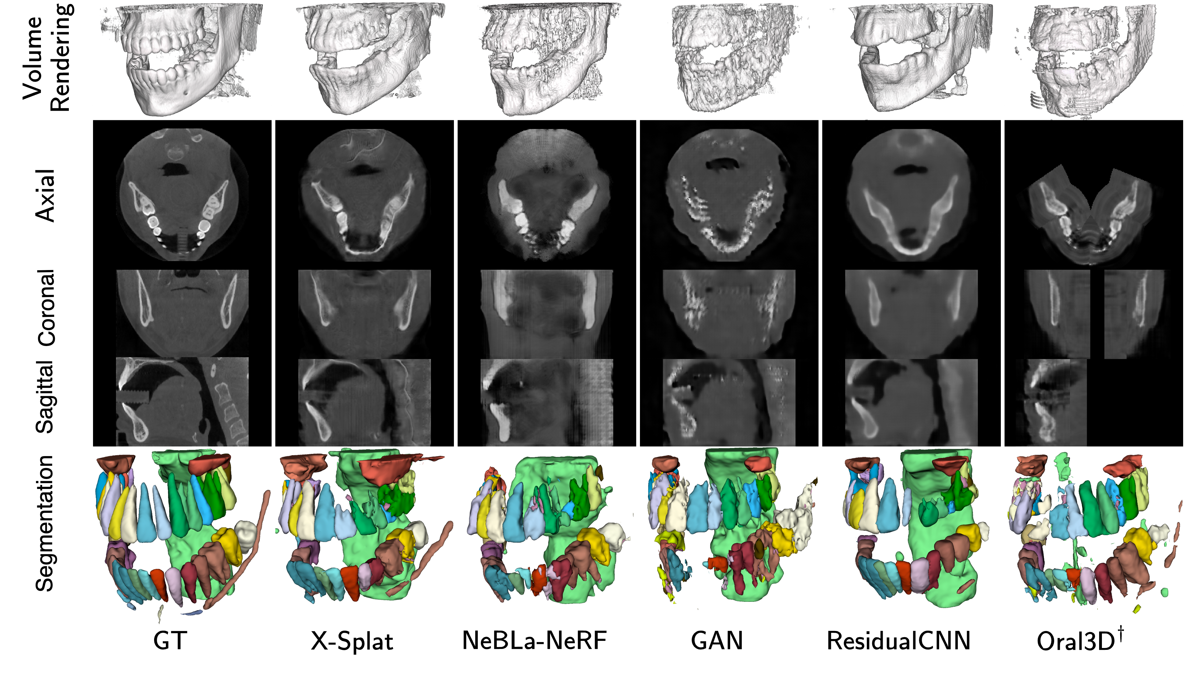
Figures 6 and 7 extend the qualitative comparison of the main paper to two additional test cases. X-Splat is the only method to recover the mandibular canal as a continuous tubular structure, visible as a curved hypodense channel in the sagittal cross-section and as a distinct labelled object in the 3D segmentation. Competing methods either omit the canal entirely or produce disconnected fragments, consistent with the reported CVR gap. The maxillary sinuses appear as clearly defined bilateral hypodense cavities in the GT Sagittal view; X-Splat reproduces partially their shape and symmetry, while NeBLa-NeRF and Residual CNN fill the sinus region with diffuse intermediate intensity and GAN introduces artifacts that obscure the boundary entirely. Oral-3D, despite oracle arch access, reconstructs only the dental sub-volume and produces no sinus anatomy. Despite strong overall anatomy recovery, X-Splat struggles to precisely reconstruct root apices, where the fine geometry may exceed the resolution of the current splat density; larger training datasets and feed-forward adaptive densification of Gaussian primitives near high-curvature boundaries remain directions for future work.

References↩︎
t.szczepanski@sanoscience.org↩︎