Object Aligner: A Configurable JSON Schema Similarity Score for Graphs, Applied to LLM Prompt Optimization
July 02, 2026
Abstract
Large language models (LLMs) are often asked to produce JSON conforming to a fixed schema, powering information extraction, tool calling, agentic planning, and knowledge-graph construction. Measuring how closely an output matches a gold reference is essential yet surprisingly hard: exact match is brittle, text similarity ignores structure, and an LLM judge is expensive, opaque, and non-deterministic. We address this with Object Aligner (OA), an open-source Python library that scores two JSON objects deterministically by recursively aligning their trees (the Hungarian algorithm for unordered collections, sequence alignment for ordered ones) and awarding partial credit at the granularity the schema declares. The Object Aligner is configured entirely through a set of JSON Schema extensions, so adapting it to a new task involves annotating a schema rather than writing code. Complex structured data, however, are rarely flat trees: records may form graphs or hypergraphs keyed by arbitrary identifiers, breaking the assumptions of prior similarity metrics. Our central contribution, referential alignment, closes this gap by inferring a bijection between gold and candidate identifiers and scoring every reference through it, so the score is invariant to relabeling. Since recovering this bijection exactly is graph isomorphism, the Object Aligner approximates it with Weisfeiler–Leman color refinement. An order-sensitive sequence regime targets ranking and planning. Since the same alignment localizes every mismatch, the Object Aligner emits ranked repair suggestions at no extra cost. Used as a reward inside the GEPA prompt optimizer, Object Aligner helps or stays neutral across all datasets.
Drchal: Object Aligner: A Configurable JSON Schema Similarity Score for Graphs Drchal: Object Aligner: A Configurable JSON Schema Similarity Score for Graphs
Object Aligner, complex structured data, large language models, prompt optimization, graph similarity score, JSON schema
1 Introduction↩︎
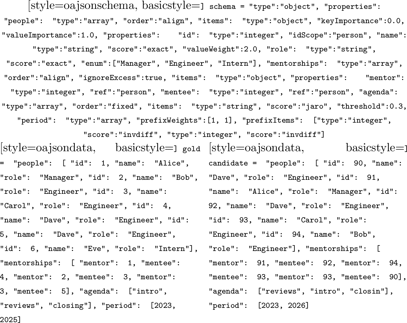
complex structured data, i.e., measuring how closely two structured objects agree, is a basic operation in many settings: automated testing, change detection between versions, record linkage, and the evaluation of machine-learning systems against reference outputs. It has become more urgent with large language models (LLMs). Along with free-form text, an LLM is often asked to return data conforming to a fixed schema (most often JSON) so that its output can be parsed, stored, and consumed directly by downstream systems: information extraction, document understanding, tool and function calling, agentic planning, and knowledge-graph construction all rely on it. JSON is among the most widely used data formats in practice, and although it is essentially a tree, cross-references between records allow it to encode general graphs and hypergraph structures (Fig. 1). Judging whether two such objects agree (for instance a model prediction against a gold reference) is therefore both common and hard: the comparison must look past cosmetic differences such as reordering or identifier renumbering and credit what is structurally correct.
When the scoring procedure itself must be controlled—reproducible and auditable—LLM-based judging is not a solution. LLM-as-a-judge [1] replaces a human evaluator with another model, but it inherits the very difficulty we are trying to escape: the judge must itself be prompted, calibrated, and validated; it is costly, noisy, and non-deterministic; it is prone to position and verbosity bias; and its verdicts are opaque, which makes them hard to audit. Generic text-similarity metrics [2]–[4] avoid these costs but discard the structure entirely. What is needed instead is a deterministic, schema-aware score that compares a prediction directly against a gold object and credits the parts it gets right.
We introduce Object Aligner (OA), a highly configurable similarity score4 for structured outputs, computed by a recursive, schema-driven alignment of gold and candidate trees that matches each node’s children with the appropriate optimal-alignment algorithm: the Hungarian algorithm for unordered collections and a sequence-alignment dynamic program for ordered ones (such as our example in Fig. 1). By design, the score is deterministic, decomposable, and schema-aware, so partially correct objects receive partial credit at the granularity declared by the schema. The comparison is driven entirely by a schema expressed as a small set of JSON Schema extensions (per-field weights, leaf comparators, and ordering and reference semantics) so adapting Object Aligner to a new task amounts to annotating a schema rather than writing code. Object Aligner ships as an open-source Python module.
Such a score has many uses; this study concentrates on one of them, prompt optimization. Coaxing an LLM to produce the correct structured output is difficult: performance is highly sensitive to how the task is phrased, which examples are shown, and how the schema and its constraints are explained. Therefore building a reliable pipeline is increasingly an exercise in prompt engineering. Prompt-optimization (PO) frameworks automate this search by iteratively proposing and refining prompts, and can match or surpass careful manual tuning at a fraction of the human effort [5].
Regardless of the method, the reward that measures candidate quality determines what the PO search can achieve: no search can optimize for quality its reward cannot see. That reward is computed over a labeled dataset and evaluated for many candidate prompts across the loop. This is exactly where the Object Aligner fits—a deterministic, decomposable structural reward—though prompt optimization is far from its only use. The common alternative of using an LLM to score candidates or to reflect on their failures is computationally demanding and non-deterministic, expensive to run at the scale a search requires, hard to reproduce and audit, and sensitive to prompt and position bias—the same problems that motivate a controlled score in the first place.
The core idea—side-by-side recursive Hungarian matching of gold and candidate trees—was described concurrently by STED [6] and ExtractBench [7] and implemented in Stickler [8]. Our publicly recorded implementation5 predates all of them, and we treat this part of the work as a simultaneous discovery. Taking this shared idea as our starting point, we chose to extend it; hence our main contributions are:
An open-source Python library implementing Object Aligner6, configured entirely through JSON Schema extensions and deployable as a drop-in reward for existing prompt-optimization frameworks such as DSPy [9], GEPA [10], and TextGrad [11].
The application of a deterministic structural score as the reward signal of a prompt optimizer. It is the first PO pipeline driven by schema-aware partial credit over nested structures, to our knowledge.
Referential alignment for (hyper)graphs: A scoring regime invariant to the relabeling of identifiers, which infers a bijection between gold and candidate identifiers and scores every reference through it, approximated with Weisfeiler–Leman color refinement [12] since recovering it exactly is graph isomorphism (Section 3.5).
Per-list sequence semantics: A per-list choice between order-agnostic matching, a monotone, insertion/deletion-aware regime suited to ranking and planning tasks, and positional tuples—fixed-arity sequences whose slots carry position-specific meaning, each with its own importance and comparator (Section 3.3).
Deterministic ranked feedback for prompt optimization: The same gold–candidate alignment that produces the score also pinpoints where the candidate departs from the gold, and emits these mismatches as repair operations—edits that would bring the candidate closer to the gold—ranked by the exact amount of score each recovers, so the optimizer is pointed at the changes that matter most, with no LLM call (Section 3.6).
An empirical study on both synthetic data, which allows us to isolate and control the specific properties of the score, and real-world datasets.7
The remainder of the paper is organized as follows. Section 2 reviews the structural similarity metrics, concurrent structured-output scorers, and prompt optimization. Section 3 defines the Object Aligner and its extensions. Section 4 describes the datasets, and Section 5 reports the experiments. Section 6 discusses the findings, Section 7 the limitations, and Sections 8 and 9 conclude and outline future work.
2 Related Work↩︎
Object Aligner builds on a long line of work on comparing structured objects and is motivated by a recent one: prompt optimizers that consume cheap, reliable reward signals. We review structural similarity first, then the concurrent structured-output scorers, and close with the prompt-optimization frameworks that define the use case.
2.1 Similarity Scoring for Structured Data↩︎
2.1.0.1 Tree edit distance.
Comparing trees is classically cast as tree edit distance (TED): the minimum-cost script of node insertions, deletions, and relabelings that turns one tree into the other [13]. For ordered trees the Zhang–Shasha algorithm computes the TED in polynomial time [14], with APTED being the current state of the art [15]. For unordered trees, the problem is NP-hard, and Zhang’s constrained edit distance restores tractability by requiring disjoint subtrees to map to disjoint subtrees, which reduces the matching of each node’s children to a bipartite assignment [16]: the closest classical relative of Object Aligner’s recursion. X-Diff applies the same restriction to unordered XML change detection [17]. All of these return an edit cost under uniform, hand-set operation costs: they have no notion of a schema, per-field importance, or graded leaf similarity.
2.1.0.2 Optimal assignment as an evaluation primitive.
The Hungarian algorithm [18] has a long history in evaluation. In coreference resolution, CEAF scores a system by maximum-weight bipartite matching between gold and predicted entity clusters [19], in contrast to link-based MUC [20] and LEA [21], and mention-based B\(^3\) [22]. Template-filling evaluation extends CEAF by one level of recursion—templates are matched on the aggregate similarity of their slot fillers [23], [24]—but remains specific to flat MUC-style templates. In computer vision, DETR uses the same matching as training loss for set prediction [25]. Most directly, the bipartite approximation of graph edit distance reduces an NP-hard comparison to a single linear assignment over node edit costs [26]. Object Aligner applies similar idea recursively to schema-typed trees, with the cost matrix computed bottom-up from configurable leaf comparators.
2.1.0.3 Semantic-graph metrics.
Invariance to identifier renumbering—the property motivating referential alignment (Section 3.5)—has been studied mainly for semantic graphs. Smatch scores two Abstract Meaning Representation (AMR) graphs by searching for a one-to-one alignment of their variables with a restart-dependent hill-climbing heuristic [27]. S2match replaces binary concept equality with graded embedding similarity [28], and Smatch++ solves the alignment optimally as an integer linear program [29]. WWLK instead compares AMR graphs through Weisfeiler–Leman (WL) node embeddings and optimal transport [30]. Discrete shared WL colors underlie the optimal-assignment graph kernel WL-OA [31], the closest prior use of joint refinement for matching vertices (cf. Section 3.5). These metrics achieve exactly the renumbering invariance Object Aligner targets, but for a single formalism: the Smatch family operates on a flat triple set, none recurses into nested values, and none exposes schema-level configuration. We make this relationship concrete by evaluating Object Aligner on AMR (Section 4.5), where Smatch’s variable alignment is the same problem that Object Aligner solves as referential matching from a schema.
2.1.0.4 Practical comparison of JSON and records.
JSON diff libraries such as DeepDiff recurse through nested objects and can ignore list order, but they pair list items greedily rather than by optimal assignment and expose only an unweighted distance with no field importance or graded leaf similarity [32]. Probabilistic record linkage is a mature precedent for declarative per-field comparison: Fellegi–Sunter-based tools such as Splink attach fuzzy comparators and weights to each field of a flat record [33], [34]. Object Aligner generalizes this declarative pattern to trees of arbitrary depth. The idea of identifying records through their references rather than their attributes is rooted in the relational model. Chen’s entity–relationship model represents a relationship as a relation keyed by the primary keys of the entities it links and, when attributes alone cannot identify a record, resolves it recursively through its relationships with other records [35]—the reference-driven disambiguation that referential alignment performs up to identifier relabeling (Section 3.5). For LLM outputs specifically, function-calling benchmarks check predicted calls by exact AST matching, recursing into argument values for type and equality but offering no graded leaf similarity, field importance, or alignment of records by reference [36], while the flexible alternative, LLM-as-a-judge [1], reintroduces the cost, noise, and calibration burden discussed in Section 1. Recent surveys likewise call for a more rigorous, reproducible LLM evaluation methodology [37].
2.2 Concurrent Structured-Output Scorers↩︎
To our knowledge, three systems developed concurrently with the Object Aligner (Section 1) target the same problem. Stickler [8], an AWS Labs library (without an accompanying paper), scores LLM outputs against Pydantic models with per-field comparators and weights; lists of structured models are Hungarian-matched, but pairs scoring below a match threshold are not recursed into and are counted as false detections in a confusion-matrix report aimed at document-processing audits. STED [6] computes a tree edit distance with Hungarian child matching at every level and embedding-based leaf costs, controlled by a handful of global weights with no schema or per-field configuration, targeting the consistency benchmarking of repeated generations. ExtractBench [7] is primarily a benchmark; its evaluator reads a per-field scoring configuration from an annotated schema but aligns arrays with an LLM call rather than an assignment solver.
Table 1 summarizes these differences, with Smatch++ included as the closest non-JSON relative. Several axes have no full counterpart in the three concurrent systems. First, none is invariant to identifier renumbering:
renumbering the identifiers of Fig. 1 changes their score even though the encoded graph is unchanged, whereas referential alignment (Section 3.5) scores every reference through an inferred
identifier bijection: among these systems, only Smatch++ offers the same guarantee (but limited to AMR graphs). Second, none lets the schema declare, per list, whether order is part of the answer: STED matches children order-agnostically throughout,
Stickler always Hungarian-matches structured lists, and ExtractBench delegates ordering to the judge LLM, whereas Object Aligner’s order keyword selects per sequence between the order-agnostic (optimal bipartite)
and order-sensitive (monotone, insertion/deletion-aware) regimes (Section 3.3). Relatedly, none treats a fixed-arity sequence as a positional tuple—slots whose meaning differs by position, each with its own
importance and comparator, aligned one-to-one by position (Section 3.3): STED and ExtractBench match such arrays interchangeably like any other list. Third, only Object Aligner emits
optimizer-ready feedback: repair operations ranked by exact score deltas derived from the match tree (Section 3.6); Stickler’s reports target human auditors, and STED returns a bare scalar. Finally, two design choices
make the Object Aligner suitable for the inner loop of prompt optimization, its motivating use case. The score is continuous, with no threshold gating (unlike Stickler), and scoring requires no embedding or LLM calls (unlike
STED and ExtractBench); rollouts can thus be scored deterministically and reproducibly, without the per-call model inference those scorers require.
3.5pt

2.3 Prompt Optimization↩︎
A prominent line of automatic prompt optimization uses LLMs as optimizers: APE generates instruction candidates and keeps the best-scoring [38], OPRO iteratively proposes prompts conditioned on the trajectory scored so far [39], evolutionary variants maintain a mutating population [40], [41], and error-driven refinement clusters failure cases into prompt updates [42]. DSPy makes the reward interface explicit: a multi-stage LM program is compiled against an arbitrary user-supplied metric [9], which its MIPROv2 optimizer maximizes by Bayesian optimization over instructions and few-shot demonstrations [43]. TextGrad instead propagates natural-language “gradients”—textual critiques of intermediate outputs—through compound systems [11]. Across all of these frameworks, the metric is supplied by the user. Where prompt optimizers have been applied to structured-output tasks, the reward has been exact-match triple F1 for knowledge-graph construction [44], exact-match parse accuracy for semantic parsing [45], or, at most, a graded span-overlap measure for flat entity extraction [46]; graded structural rewards such as Smatch or graph edit distance have appeared only as reinforcement-learning signals for weight tuning [47], [48]. To the best of our knowledge, no published prompt-optimization pipeline has driven the search with schema-driven partial credit over nested structures.
We adopt GEPA [10] as the optimizer in all the experiments for two reasons. First, it is sample-efficient: candidate mutations are screened on minibatches rather than full validation sweeps, and new candidates are drawn from a Pareto frontier over individual training instances, preserving diversity. The authors report that it outperforms MIPROv2 and matches or beats GRPO-style reinforcement learning at a fraction of the rollouts. Second, it is reflective: like TextGrad and other feedback-driven optimizers, it updates prompts from natural-language critique, but here that critique is returned by the metric itself: each mutation is proposed by an LLM that reads execution traces together with textual feedback from the metric, so its metric interface is a (score, feedback) pair rather than a bare scalar. Object Aligner exactly fills this interface: a deterministic score for Pareto bookkeeping and structurally faithful repair feedback for reflection (Section 3.6).
3 Object Aligner↩︎
This section provides a description of the Object Aligner. We first fix the data model and the two-phase scoring it uses (Section 3.1), and then instantiate it for the primitive, sequence, and map nodes (Sections 3.2–3.4). We then develop three extensions that are the focus of this paper: order-sensitive sequence alignment with insertion/deletion support (Section 3.3), referential alignment for (hyper)graphs, which compares structured outputs up to identifier renumbering (Section 3.5), and deterministic, optimizer-shaped feedback that turns the score into a learning signal (Section 3.6). We close with the formal properties and cost of the procedure (Section 3.7).
3.1 Overview and data model↩︎
The Object Aligner takes a gold object \(g\), a candidate (predicted) object \(p\), and a schema \(S\), and returns a similarity score \(\mathrm{s}(g, p \,;\,S) \in [0, 1]\), where \(1\) denotes a perfect match and \(0\) a complete mismatch. By design, the score is (i) deterministic—the same inputs always yield the same number8; (ii) schema-aware—the comparison is driven entirely by \(S\), so partially correct objects receive partial credit at the granularity the schema declares; and (iii) decomposable—the top-level score is an explicit weighted aggregate of child scores, which makes feedback possible (Section 3.6).
We model both \(g\) and \(p\) as value trees. A value is either a primitive (a string, a number, or a boolean), the empty value \(\bot\), a
sequence (an ordered tuple of values), or a map (a JSON object, a finite set of key–value pairs with distinct keys). The schema \(S\) is an annotated tree of the same shape: each node fixes
the expected type and the local scoring choices—which primitive comparator to use, how to weight children, whether a sequence is order-sensitive, and whether a primitive acts as an identifier. Our implementation represents the value trees as JSONs, whereas
the schema takes the form of JSON Schema extensions documented in Appendix 10.
The alignment descends \(g\), \(p\), and \(S\) in lockstep, producing a score at every node and aggregating upward to the root. Fig. 1 shows a concrete schema for the running example, a small organization chart: six people in one identifier scope, directed mentorships between them, an order-sensitive agenda, and a
period year tuple. The schema also exercises several Object Aligner-specific extensions beyond the plain JSON Schema (e.g., keyImportance, valueWeight, enum,
prefixItems, and fuzzy score comparators).
The scoring at every internal node proceeds in two phases. In the alignment phase, Object Aligner fixes a correspondence between the children of \(g\) and those of \(p\)—a partial matching that says which gold child is compared against which candidate child. In the scoring phase, it aggregates the per-pair child scores over the fixed correspondence into a single number in \([0,1]\).
The cost that drives the matching depends on the node type and schema configuration. For sequences, the elements are matched by either the Hungarian algorithm or the order-sensitive dynamic programming approach. For a map, matching
involves only the Hungarian algorithm over key similarity. Moreover, referential alignment (Section 3.5) introduces identifiers and references, analogous to primary and foreign keys in relational databases.
Primitive types (leaves) are scored directly. A node where one or both sides are the empty value \(\bot\) is also scored directly: two empties agree (score \(1\)), whereas a value present on
only one side scores the schema’s nullScore (default \(0\)). Algorithm 2 states the dispatch, and the following subsections describe each case.
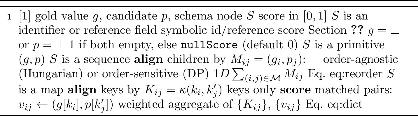
3.2 Primitive types↩︎
A primitive node carries a similarity function \(\sigma:\mathcal{V}\times\mathcal{V}\to[0,1]\) on primitive values \(\mathcal{V}\). For strings, \(\sigma\) is a configurable comparator: exact match \(\mathbb{1}[g=p]\), a normalized edit- or sequence-distance similarity, such as Jaro [49] or Levenshtein [50]. For numbers, we may choose an exact match, inverse difference (\(1/(1+|g-p|)\)); Booleans are compared exactly. Any primitive type can be scored using a user-supplied comparator function (e.g., semantic embedding similarity for text).
3.3 Sequences↩︎
A sequence node compares two tuples \(g_1,\dots,g_n\) and \(p_1,\dots,p_m\) whose elements share a child schema. The per-pair matching cost is the full recursive score \(M_{ij}=\mathrm{s}(g_i,p_j)\), so whatever similarity the children carry (nested maps, further sequences) propagates into the correspondence. The Object Aligner implements two regimes:
3.3.0.1 Order-agnostic.
When the element order is irrelevant (a set of entities), the alignment is the optimal bipartite matching: pad \(M\) to a square \(d\times d\) matrix (\(d=\max(n,m)\)) with zero rows/columns for absent elements and choose \[\pi^\star = \mathop{\mathrm{arg\,max}}_{\pi} \sum_{i=1}^{d} M_{i,\pi(i)}, \label{eq:assignment}\tag{1}\] the maximum-weight assignment, solved optimally using the Hungarian algorithm [18]. Writing \(\mathcal{M}=\{(i,\pi^\star(i)) : M_{i,\pi^\star(i)}>0\}\) for the genuinely matched pairs, the score is \[\mathrm{s}(g,p\,;\,S) = \frac{1}{D}\sum_{(i,j)\in\mathcal{M}} M_{ij}. \label{eq:reorder}\tag{2}\] An unmatched gold element is missing, and an unmatched candidate element is excess; each occupies a slot scoring \(0\). The denominator \(D = |\mathcal{M}| + n_{\mathrm{miss}} + n_{\mathrm{exc}}\) counts the matched pairs plus the penalized unmatched elements, and whether the missing or excess elements count toward \(D\) is schema-configurable.
3.3.0.2 Order-sensitive.
When the order is itself part of the answer (steps of a plan, ranked items), admissible matchings are restricted to the monotone ones, which preserve the left-to-right order while allowing insertions and deletions. The optimal monotone matching is computed by the standard sequence-alignment dynamic program and scored under the same denominator convention as in Eq. 2 . Unlike the order-agnostic regime, a transposition breaks the monotone path and is penalized on both elements.
3.3.0.3 Tuples and prefixes.
The two regimes above treat a sequence as unbounded. In practice, we often work with tuples: a fixed number of positional slots whose meaning differs by position (a coordinate triple, a labeled header), so each slot deserves its own importance rather than being matched interchangeably. We unify both as a prefix: a fixed-arity positional head followed by an optional variable-length tail. The prefix elements are aligned one-to-one by position; with per-position importances \(v_1,\dots,v_a\) (\(a\) the prefix arity, uniform by default) their scores are combined as \[s_{\mathrm{pre}} = \frac{\sum_{k=1}^{a} v_k\, \mathrm{s}(g_k, p_k\,;\,S)}{\sum_{k=1}^{a} v_k}, \label{eq:prefix-score}\tag{3}\] whereas the tail is aligned by one of the two regimes above into \(s_{\mathrm{rest}}\) (a pure tuple is just the empty-tail case). The two blend as \[\mathrm{s}(g,p\,;\,S) = \frac{w_p\, s_{\mathrm{pre}} + w_r\, s_{\mathrm{rest}}}{w_p + w_r}, \label{eq:prefix}\tag{4}\] with prefix and tail importances \(w_p,w_r\).
3.4 Maps↩︎
The map is aligned by its keys alone. Given gold keys \(k_1,\dots,k_n\) and candidate keys \(k'_1,\dots,k'_m\), the alignment is optimal bipartite matching (Eq. 1 ) on the key-similarity matrix \(K_{ij} = \kappa(k_i, k'_j)\) where \(\kappa\) is a key comparator (exact, fuzzy, or user-defined). Note that the values are not consulted when choosing which keys pair: maps are matched by their labels only. This is deliberate. The keys already identify what each entry represents, so they suffice to decide what is compared to what, and matching values would force the user to weight keys against values: two scales with no obvious, schema-independent trade-off. Keys fix the correspondence, the values then grade it. If the key-only rule is too limiting, the collection can be modelled as an order-agnostic sequence of \(\langle\text{key},\text{value}\rangle\) tuples (Section 3.3), recovering the relational view of a map as a matched set of typed pairs.
Given the matched key pairs \(\mathcal{M}=\{(i,\pi^\star(i)) : K_{i,\pi^\star(i)}>0\}\), the scoring phase recurses on the paired values, \(v_{ij}=\mathrm{s}(g[k_i],p[k'_j])\) (unmatched keys contribute \(0\)), and aggregates a key term and a value term: \[\begin{align} s_{\mathrm{key}} &= \tfrac{1}{d}\textstyle\sum_{(i,j)\in\mathcal{M}} K_{ij}, \\ s_{\mathrm{val}} &= \frac{\sum_{(i,j)\in\mathcal{M}} \omega_i\, v_{ij}}{\sum_{i=1}^{d} \omega_i}, \\ \mathrm{s}(g,p\,;\,S) &=
\frac{w_K\, s_{\mathrm{key}} + w_V\, s_{\mathrm{val}}}{w_K + w_V}, \label{eq:dict}
\end{align}\tag{5}\] with key weight \(w_K\), value weight \(w_V\), and per-property weights \(\omega_i\). The Object
Aligner’s default \(w_K=0\) (schema keyword keyImportance) treats keys as fixed scaffolding therefore, only the values are scored. Setting \(w_K>0\) suits
open-vocabulary extraction, where the model also chooses the keys and obtaining a key right is itself part of the task.
3.5 Referential alignment↩︎
Many structured outputs are really (hyper)graphs: some records carry an identifier at which other parts point back. The identifier values are meaningless; two correct extractions may number their records differently (Fig. 1) and a primitive-by-primitive comparison would punish this as an error. We want a score invariant to relabeling of identifiers. Referential alignment does this: the schema marks one primitive field as an identifier and others as references to it, and Object Aligner infers a bijection between gold and candidate identifiers and then scores every reference through it.
3.5.0.1 Scopes, records, and references.
The schema keywords are idScope and ref (Fig. 1), which behave like primary and foreign keys. An idScope on a primitive inside a sequence names a scope whose items are its
records; a ref of the same type points to a named scope from anywhere. In the example, the person scope has six records (the people, keyed by id), and each mentorship references two
of them (mentor and mentee). Identifiers and references are matched symbolically through the bijection, not by raw values, so their primitive comparator is ignored.
3.5.0.2 Deriving the bijection.
To recover the bijection for a scope, we align its gold and candidate records as an order-agnostic sequence (Eq. 2 ): writing \(d_i\) for the gold records and \(d'_j\) for the candidate ones, form the record cost matrix \(C_{ij}=\mathrm{s}(d_i, d'_j)\), solve the assignment (Eq. 1 ), and read the bijection \(\pi:\text{gold ids}\to\text{candidate ids}\) off the optimal pairs (partial if the sides differ in size—unmatched gold ids map to \(\bot\) and references to them score \(0\); excess candidate ids stay outside the bijection’s image, so any reference pointing at one cannot match its gold counterpart and scores \(0\)). Deriving the bijection involves two steps. First, we mask the scope’s own id field: its value is arbitrary, so comparing it would only penalize the right pairing. Instead, we treat it as a perfect match (score \(1\)), so it drops out of the comparison, and records are paired by everything except their id—in the example, by name and role, which already pair each gold person with the right candidate. Second, we never compare a reference by value, while the scope it points to is still unresolved, as that would use a bijection we have not yet computed. Thus, we resolve scopes in dependency order (topological sort, lexicographic tie-break for determinism). A reference into the same scope, and any cycle of mutually referential scopes, has no such order, so there we warn and fall back to property-only alignment.
3.5.0.3 Breaking ties by structure.
Masking ids can leave the assignment underdetermined: when two records agree on all their other attributes (the two Dave/Engineer twins in the example) their rows in \(C\) are
identical and attributes give no reason to prefer one pairing. The twins may still differ in structure: one Dave is mentored by Alice, and the other by Carol (Fig. 4). Resolving this exactly
is again graph isomorphism, far costlier than the cubic Hungarian assignment that we already pay. We therefore use a near-linear \(1\)-dimensional Weisfeiler–Leman (1-WL) color refinement [12], [51] as a tractable approximation to that test. It
gives each node a color and repeatedly refreshes it from its neighbors’ colors until structurally distinct nodes are separated.
The colors must be comparable across the two sides, and refining each graph on its own does not give that: 1-WL numbers colors in the order signatures appear, so gold’s color \(3\) and candidate’s color \(3\) are unrelated. We therefore refine jointly: one graph per side—a node per record, and a directed edge for each reference linking two records, labeled by the scalar fields of the reference-bearing record (its
carrier); in the example each mentorship is a single mentor \(\to\) mentee edge between two person nodes—over their disjoint union \(\mathcal{G}_g\sqcup\mathcal{G}_c\) (gold, candidate; Fig. 4), each round recomputing a vertex’s signature from its own color and the sorted multiset of its incident-edge descriptors,
\[\mathrm{sig}^{t+1}(v) = \big(\, c^{t}(v),\;\mathrm{sort}\,\{\!\!\{\, (\delta, f, \ell, c^{t}(u)) \,\}\!\!\} \,\big), \label{eq:wl-refresh}\tag{6}\] where the multiset
ranges over all incident edges \((v,u,f,\ell)\in\mathcal{E}\) in both directions \(\delta\in\{\text{in},\text{out}\}\), each contributing its direction \(\delta\) (for a mentorship, whether \(v\) is the mentor or the mentee end), the relationship’s label \(f\) (here
mentor \(\to\) mentee), an edge label \(\ell\), and the neighbor’s color \(c^{t}(u)\). The label \(\ell\) is compared by exact equality, so it carries only what is already settled on both sides—the carrier’s own scalar fields together with any of its references into already-resolved scopes—while fuzzy attributes9 and references into the still-unresolved current scope are left out. In the running example, a mentorship holds nothing but its two references, so \(\ell\) is empty and the twin Daves separate only through their neighbors’ colors. Were each link to also record a since year—say Alice \(\to\) Dave since 2019 and Carol \(\to\) Dave since 2021—their two incoming edges would carry \(\ell=\texttt{2019}\) versus \(\ell=\texttt{2021}\), splitting the look-alike Daves by this exact-equal scalar in a single round, without the extra refinement their mentors’
differing colors otherwise require.
A single intern table shared by both sides (Relabel, Algorithm 3) maps each round’s signatures to integer colors \(c^{t+1}(v)\), so identical signatures
get the same color on gold and candidate—comparable by construction, with no seed, anchor, or learned embedding, and without ever consulting the bijection we derive (no circularity). This joint relabeling is the standard Weisfeiler–Leman construction,
concordant across graphs by design [51]. The closest prior method to use such discrete shared colors for
matching vertices is the optimal-assignment kernel WL-OA [31]. We depart from it in two ways: our graphs carry directed, relation- and
scalar-labeled edges with references into already-resolved scopes, and the colors enter only as an infinitesimal tie-break (below) rather than as the assignment objective itself. In Fig. 4, our construction pins the twins, and
in the final round, each candidate Dave carries the color of its gold match.
In the default tie-break mode, the colors enter the cost matrix only as an infinitesimal bonus \(\epsilon\,b_{ij}\), with \(b_{ij}=\mathbb{1}[\,\text{colors agree}\,]\) and \(\epsilon\) below the smallest gap between distinct attribute costs; therefore, the structure breaks only exact ties and never overrides what the attributes decide. Object Aligner also implements an optional blend mode that seeds the refinement from each record’s attributes and mixes structure into the cost at a fixed weight rather than as a tie-break, which suits cases where attributes already separate most records. We omit its details and experiments for brevity.


3.5.0.4 Scoring references.
With the bijection in hand, the main alignment pass (Algorithm 2) treats identifier fields as labels worth \(1\) and scores a reference as correct if and only if it points, through the
inferred mapping, at the same record the gold reference does (and that target exists among the candidate ids; otherwise it scores \(0\)). In Fig. 1 the masked name/role comparison, with the
twins split by structure, recovers \(\pi=\{1\!\mapsto\!91,2\!\mapsto\!94,3\!\mapsto\!93,4\!\mapsto\!92,
5\!\mapsto\!90,6\!\mapsto\!\bot\}\), under which every mentorship matches exactly despite every id differing; the object still loses credit for the omitted Eve and the perturbed agenda/period, for
a final \(\mathrm{s}=0.77\).
3.6 Optimizer feedback↩︎
A scalar reward tells an optimizer how well a prompt does, but not what to change. Because Object Aligner’s score is decomposable, we can answer the second question deterministically and without an LLM: the same alignment that produced the score also localizes the deficit, which we render as a compact, prescriptive feedback string suitable for the natural-language reflection slot of a reflective prompt optimizer such as GEPA [10] or TextGrad [11]—in DSPy [9], for instance, GEPA is exposed as an optimizer whose metric returns this textual feedback alongside the scalar score. This contrasts sharply with LLM-as-judge feedback [1], which is noisy, non-deterministic, and must be prompted and calibrated.
Walking the match tree, every imperfect leaf or structural mismatch becomes a repair operation with an associated score delta—the amount of total score recovered by fixing it. For a child contributing with effective weight \(c_w\) and value score \(s_w\), the delta is \(\Delta(\mathrm{op}) = c_w\,(1 - s_w)\), and, under the fixed assignment chosen by alignment, summing these deltas over the full set \(\mathcal{O}\) of repair operations accounts for the entire score deficit exactly, \(\sum_{\mathrm{op}\in\mathcal{O}} \Delta(\mathrm{op}) = 1 - \mathrm{s}(g,p\,;\,S)\), that is, the gap between a perfect score and the one achieved. Operations are typed (primitive replacement, missing/extraneous key, fuzzy key rename, missing/excess sequence element, wrong reference, whole-subtree replacement, etc.) and each carries a path to its location.
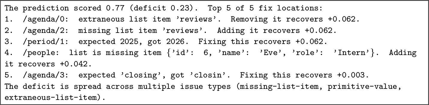
Operations are ranked by \(\Delta\), the top \(K\) are kept (those below a minimum delta are dropped), and each is rendered through a per-type template. A trailing synthesis line names the dominant error category when one type accounts for most of the displayed deficit. The per-type templates are configurable. For the running example of Fig. 1 (scored at \(0.77\)), the feedback rendered by the default templates is shown in Fig. 5. Each line is a deterministic template substitution, and the deltas are derived from the exact decomposition described above.
3.7 Properties and cost↩︎
Object Aligner is deterministic and reproducible: every choice point (assignment, WL relabeling, tie-breaks) is resolved by a canonical, seed-independent rule. The score is bounded in \([0,1]\) and awards partial credit at schema granularity. It is decomposable, which precisely enables the attribution and feedback of Section 3.6.
The cost is dominated by per-node work. A sequence or map alignment of arity \(d\) solves one assignment problem, \(O(d^3)\), over an \(O(d^2)\)-entry matrix whose sequence entries are recursive alignments (a map instead scores cheap key comparisons, recursing only on the \(\le d\) matched pairs); order-sensitive sequences replace the assignment with an \(O(nm)\) dynamic program. Referential alignment adds one assignment per scope plus WL refinement, which costs \(O\!\big(R\,(|V|+|E|)\big)\) with \(R\le|V|\) rounds over the scope’s reference graph. Summed over the tree, the cost is dominated by the assignments, each cubic in its collection’s local arity \(d\), where \(d\) is the number of matched siblings—fixed and small for an object’s keys, so only list lengths grow with the document. A single such list is already \(O(n^3)\), and nesting growing lists multiplies this further, but in practice these lists stay short and shallow, so the cost remains a non-issue.
4 Datasets↩︎
The following datasets are used in Section 5 to demonstrate the Object Aligner properties, focusing mainly on Referential Alignment (RA) and order semantics. The list contains both synthetic (Org2Graph and Facts2Order) and real-world data. We briefly introduce each dataset; worked examples, schemas, and native task metrics are deferred to the per-dataset appendices (Appendix 11, native metrics in Appendix 14). Real-world datasets were converted to JSON under an OA schema and, in some cases, reframed for our needs.
4.1 Org2Graph↩︎
In natural information extraction corpora, the difficulty of recovering referential structures is tangled up with parsing, domain vocabulary, and annotation noise, so they cannot isolate why referential alignment helps or fails.
Org2Graph (O2G) is a synthetic generator that converts this difficulty into controlled variables. Each instance is a templated natural-language paragraph describing a fictional organization, and the task is to extract the graph it describes as JSON with
five scopes: people and companies are records carrying identifiers, and employment, acquaintance, and partnership records link them through references, foreign-key style. Records and links
carry one categorical property each (title, industry, role, and the two relation types). Because the paragraph is rendered from the gold graph (every link surfaces as exactly one sentence) extraction is unambiguous by
construction. Fig. 15 (Appendix 12) shows a small instance including gold JSON output.
Three parameters control where the difficulty lies; each scope draws its categorical values from a fixed codebook (its vocabulary of allowed entries, orcodes). Twin density sets the fraction of records that are
property-twins—identical in every scored attribute, thus telling them apart, and hence routing references correctly, requires the reference structure itself. Within a scope, exactly one set of twins shares identical scored attributes, whereas
every other record maintains a distinct combination of them. Value obfuscation replaces the readable codebook entries with opaque codes under a fixed legend never shown to the model (the paragraph says “engineer,” the gold value is
T07), so an optimizer can recover the vocabulary only by aggregating evidence across examples. Vocabulary width sets each scope’s codebook size (\(24/20/20/12/12\) vs.\(6/6/6/3/3\)); narrow codebooks make property-twins frequent.
4.2 Facts2Order↩︎
Validating order sensitivity requires a task whose correct order is unique, stated explicitly in the input, and inexpensive to corrupt by a measured amount. Facts2Order (F2O) is a synthetic generator built to satisfy these properties. Each instance lists \(N\) short sentences, each stating one sortable key for a named entity (an integer quantity, a date, or an ordinal word). The task is to output the index permutation that sorts the items by their key (Fig. 18). The generator exposes a few independent parameters, and the study instantiates several configurations that differ in their settings. The number of items \(N\) fixes the length of the permutation to recover; we use different values of \(N\) across experiments (exact ranges in Section 5.1 and Section 5.4). The key type is an integer quantity, a date, or an ordinal word. Each instance may carry a variable number of irrelevant distractor sentences that state no sortable key, and merely pad the input. Finally, the sort key is presented in one of two regimes: stated, where the key is the lone numeric clause on each item, or hidden, where each item additionally carries \(2\)–\(3\) numeric decoy clauses on other attributes (e.g., a price in dollars, a length in centimeters) whose values are unconstrained, with the numeric clauses shuffled per item, so the key is never identifiable as the lone number and the model must discover which measure to sort on. Keys are drawn distinctly, so the gold order is unique, while the distractor sentences and decoy clauses leave it untouched. Because gold and candidate are index permutations, disorder is exactly measurable via the Kendall distance [52] (the minimum number of adjacent transpositions between two orderings), so corruptions can be dosed.
4.3 SciERC↩︎
SciERC [53] annotates \(500\) computer-science abstracts with scientific entities, coreference clusters, and typed
relations, which is our natural-text extraction benchmark, where difficulty arises from parsing and domain vocabulary. The target output is a graph: entities as nodes joined by reference-linked relations, extracted from
the abstract as JSON. A worked instance is in Fig. 10 (Appendix 11.1). A simplified form is used. Because reproducing exact character offsets is poorly suited to the
text-generation nature of decoder-only LLMs [54], we drop all span offsets and keep only surface text: each coreference cluster becomes one entity whose
mentions array holds its surface forms (its closed-vocabulary type, one of six, by majority vote). The raw annotations carry no entity identifiers, so we assign each entity a synthetic id (e0,
e1, …) in the cluster first-occurrence order purely to link the relation endpoints. The original mention-pair relations are projected to the cluster level (one of the seven closed predicates), discarding any relation whose
endpoints fall outside a cluster. We use original splits with no subsampling (\(349/50/100\) train/val/test).
4.4 BioRED↩︎
BioRED [55] is a document-level biomedical relation-extraction corpus of PubMed abstracts preprocessed into the same graph output as SciERC (Section 4.3)—coreference-cluster entities joined by reference-linked relations. Its distinctive feature is that each gold entity id is an opaque normalized concept accession not derivable from the
abstract, so relations must, in principle, be routed by referential alignment rather than literal-id matching. We draw a seeded \(50/50/100\) train/val/test split, with train and val subsampled from BioRED’s train/dev
pools, and the test split is the full BioRED test split. See details in Appendix 11.2.
4.5 Bio AMR↩︎
The Bio AMR Corpus [56] annotates biomedical sentences (cancer-related PubMed text) with Abstract Meaning Representation [57] graphs: each sentence maps to a rooted, directed graph of concept nodes and labeled edges. Like BioRED (Section 4.4), AMR’s variable names
are arbitrary and hidden, so referential alignment alone can carry out relation routing. Bio AMR is the purest case: the same concept recurs on many nodes, so content individuates nothing, and structure does all the work. We convert each gold PENMAN graph
into a JSON object of nodes and relations, dropping the source variable letters so that the model emits its own arbitrary node ids and only the graph structure is scored; a worked instance is shown in Fig. 12 (Appendix 11.3). The registered schema scores this referentially and pairs with literal-id strict ablation (Appendix 11.3),
which measures how much of the score referential alignment carries. We draw a seeded, unstratified \(100/100/200\) train/val/test subsample of the corpus.
4.6 NATURAL PLAN (Trip Planning)↩︎
This dataset and the one that follows target OA’s order semantics. NATURAL PLAN [58] is a natural-language planning benchmark. We use its
Trip Planning task, which asks for a strictly ordered itinerary—a sequence of cities to visit, each for a given number of days, reachable only over a stated set of direct flights. Unlike the synthetic Facts2Order (Section 4.2), the gold order here is imposed by a genuine planning constraint rather than designed in, so a correct plan must obtain both the set of stays and their sequence right. Each instance’s input
context is based on the day budget, the per-city stays and meeting windows, and the direct-flight list; the gold output is taken straight from the released cities/durations fields (Fig. 13, Appendix 11.4). We draw a difficulty-stratified \(100/100/200\) train/val/test split keyed on the number of cities (\(3\)–\(10\)).
4.7 ROCStories↩︎
ROCStories [59] is a corpus of five-sentence everyday commonsense stories. The correct order is fixed by narrative coherence in real text rather
than designed in by sortable keys, so recovering it demands commonsense reasoning. We retain only stories that segment into exactly \(N=5\) sentences; the input context presents those sentences scrambled and
labeled \(1..N\), and the gold output is the index permutation that restores the original reading order, emitted as a JSON index list (Fig. 14, Appendix 11.5). The data key is deliberately neutral (indices, not order), so neither schema nor seed prompt hints that the task is reordering. We draw a \(100/100/200\) train/val/test split (all instances are \(N=5\)). See more details in Appendix 11.5.
5 Results↩︎
We evaluate the Object Aligner in two stages. An intrinsic study (Section 5.1) validates its two novel mechanisms with no LLM in the loop, in the perturbation-based design of STED [6]: the score must stay high under benign corruptions of the gold and fall, in proportion, under harmful ones. Because STED already validates the machinery, the two metrics share (Hungarian-style order-invariant matching above all) our experiments target only Object Aligner’s additions: referential alignment (RA, Section 3.5) and the order-sensitive sequence regime (Section 3.3). An extrinsic study (Section 5.2–5.5) measures what these mechanisms buy as the reward and feedback signal driving prompt optimization (GEPA [10]).
5.1 Intrinsic validation of the alignment mechanisms↩︎
The setup is simple: a deterministic generator produces gold outputs, controlled corruptions damage them, and we measure how the score \(\mathrm{s}(g,p\,;\,S)\) responds (AUROC, rank correlations). A good score must do two things at once: stay constant under changes that preserve meaning and drop in proportion to genuine damage. RA must ignore identifier relabeling yet register every structural edit, and the sequence regime must grade reorderings yet degrade gracefully when items are dropped or inserted.
5.1.0.1 Invariance to relabeling.
Referential alignment promises that the score does not depend on how a candidate numbers its records: identifiers are matched through the inferred bijection \(\pi\), not by value (Section 3.5). We generate \(100\) gold Org2Graph graphs (Section 4.1) in the plain-narrow configuration, with sizes, edge densities, and twin density \(t\sim U[0,1]\) drawn at random (Algorithm 16, Appendix 12), and for each emit five exact copies under independent identifier relabelings (\(500\) pairs). Each copy is graph-isomorphic to its gold, so a relabel-invariant score must give all five exactly \(1\); the per-gold variance is the diagnostic. RA passes exactly (score \(1.000\), variance \(0\) on all \(100\) golds) even on the nine where every record is a property-twin and the bijection is pinned only by the reference
structure (see Fig. 15, Appendix 12). The plain ablation (idScope/ref dropped, identifiers compared by value—our stand-in for any
reference-unaware metric) averages \(0.738\) with per-gold variance up to \(5.5\times10^{-3}\): a flawless output forfeits a quarter of its credit, by an amount that depends on the arbitrary
choice of identifiers—exactly the noise a score should not inject.
5.1.0.2 Sensitivity to damage.
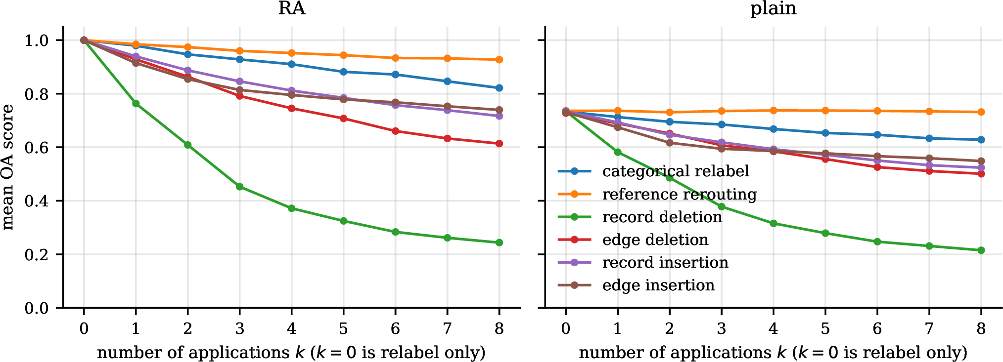
Invariance alone is trivial; therefore, the second experiment checks that RA still falls, in proportion, under genuine damage. On \(100\) fresh golds we apply a single edit type \(k{=}0,\dots,8\) times on top of a relabeled copy (\(k{=}0\) is the relabel alone): recoding a categorical value, rerouting a reference, deleting or inserting a record, or an edge—\(5400\) pairs (Algorithm 17, Appendix 12). RA starts at \(1.0\) and decreases monotonically with \(k\) under every operation (Fig. 6, left; per-operation Spearman \(-0.66\) to \(-0.89\), Table 5 in Appendix 12), and separates damaged from clean almost perfectly (AUROC \(0.996\)); the residual is correct, not noise—\(42\) of the \(4800\) edited candidates, mostly reroutes between property-twins, are graph-isomorphic to their gold and correctly scored \(1\). Plain separates significantly worse (AUROC \(0.835\)), and reference rerouting shows why (Fig. 6, right): the one edit that corrupts the graph without touching any record’s attributes moves only RA (\(1.00\!\to\!0.93\) over eight reroutes; Spearman \(-0.660\)), while plain remains flat (\(0.74\!\to\!0.73\); \(-0.011\))—the damage most specific to graph extraction is precisely the damage it cannot see. A control sweep without the relabel confirms that this gap is specific to relabeled identifiers, not the edits themselves: with identifiers matching by value, RA and plain nearly coinciding except under reference rerouting and categorical relabel (data omitted for brevity).
5.1.0.3 Sequence regime.
The sequence regime (Section 3.3) claims to grade order: a nearly-sorted output must outscore a scrambled one. On Facts2Order (Section 4.2)—configured with the item count drawn per instance as \(N\sim U\{3..12\}\), the key type drawn uniformly from {integer, date, ordinal}, \(0\)–\(3\) irrelevant distractor sentences, and the stated-key regime (no numeric decoys). OA scores the index permutations directly, so the surface sentences are ignored. We corrupt \(300\) gold orderings in two ways. The first is pure reorderings: adjacent transpositions up to a target Kendall distance, block reversals, and moves. The second is length-changing edits of the next paragraph. Together these yield \(4639\) pairs (generation: Algorithm 19; worked instance: Fig. 7). Each pair is scored in four ways: the sequence alignment under test; the order-agnostic set alignment (Hungarian matching of the label bag), standing in for STED-style matching; exact match (Perfect-Match Ratio); and Kendall \(\tau\), the graded reference one would hand-pick for this task (\(0\) on any non-permutation). On pure reordering the sequence score falls smoothly with Kendall distance (see Table 2; Spearman \(-0.706\)), while separating sorted from corrupted perfectly (AUROC \(1.000\)). The exact match also separates perfectly—it is \(0\) on every corrupted candidate by construction—but offers no gradient. The set score is exactly constant at \(1.0\) for every pure reordering (the label bag never changes): zero order signal, with AUROC \(0.705\) owing to incidental length changes alone. Kendall \(\tau\) is graded, as designed (Spearman \(-0.621\)); OA’s sequence alignment tracks this task-specific reference without being built for the task. Fig. 20 (Appendix 12) shows this behavior graphically.
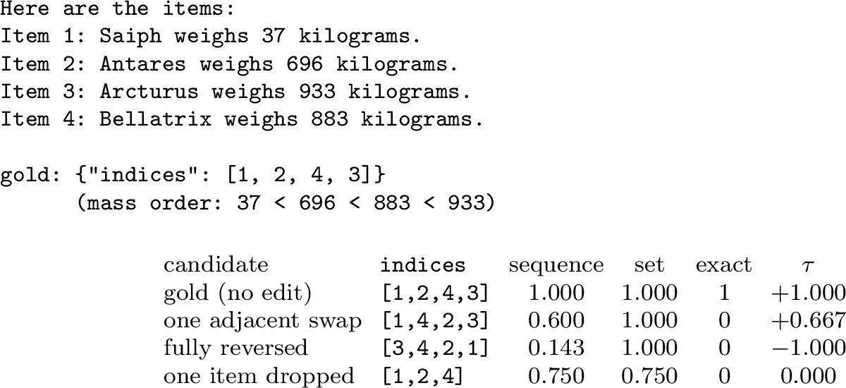
Models also drop or add new records; therefore, we further delete or insert \(k{=}1..3\) items per candidate (insertions duplicate existing ones). A single dropped item sends both the exact match and Kendall \(\tau\) to \(0\): Kendall \(\tau\) is undefined between orderings of different item sets (and scores \(0\)), and the exact match trivially fails on any length change. Instead the OA’s sequence alignment loses credit in proportion to the edit count through its gap-aligned denominator (Section 3.3). Under these pure length-changing edits (no accompanying reordering), the set score coincides with the sequence. Nevertheless, across both axes, the sequence is the only scorer that stays graded (Table 2), using the same generic, schema-driven machinery that scores every other structure in the Object Aligner.
| Corruption | sequence | set | exact | Kendall \(\tau\) |
|---|---|---|---|---|
| none (\(d{=}0\), gold) | \(1.000\) | \(1.000\) | \(1.000\) | \(1.000\) |
| \(d{=}1\) | \(0.737\) | \(1.000\) | \(0.000\) | \(0.852\) |
| \(d{=}2\) | \(0.641\) | \(1.000\) | \(0.000\) | \(0.751\) |
| \(d{=}3\) | \(0.581\) | \(1.000\) | \(0.000\) | \(0.772\) |
| \(d{=}4\) | \(0.538\) | \(1.000\) | \(0.000\) | \(0.748\) |
| \(k{=}1\) | \(0.842\) | \(0.842\) | \(0.000\) | \(0.000\) |
| \(k{=}2\) | \(0.684\) | \(0.684\) | \(0.000\) | \(0.000\) |
| \(k{=}3\) | \(0.575\) | \(0.575\) | \(0.000\) | \(0.000\) |
| \(k{=}1\) | \(0.867\) | \(0.867\) | \(0.000\) | \(0.000\) |
| \(k{=}2\) | \(0.769\) | \(0.769\) | \(0.000\) | \(0.000\) |
| \(k{=}3\) | \(0.692\) | \(0.692\) | \(0.000\) | \(0.000\) |
5pt
5.2 Extrinsic study: setup↩︎
We study the Object Aligner in the role it was originally designed for: a deterministic reward (and, optionally, a deterministic feedback signal) inside a prompt-optimization loop.
5.2.0.1 Optimizer and models.
We use a single optimizer, GEPA [10]: our grid of datasets, ablations, arms, and seeds makes a second optimizer computationally prohibitive, and GEPA is a
strong representative—state of the art (surpassing MIPROv2 [43]), sample-efficient (up to \(35\times\) fewer rollouts than
GRPO), and a standard optimizer of the popular DSPy framework [9]. GEPA is a reflective prompt optimizer that iteratively rewrites a task prompt. It maintains a
Pareto frontier of candidate prompts over the individual training instances and proposes each mutation from an LLM reflection step that reads execution traces. Candidates are screened on small reflection minibatches (size three) rather than full validation
sweeps. The reflection (proposer) LM is a frozen GPT-5 model (gpt-5-2025-08-07) [60]: pairing the reflector with a strong frontier model is
the recommended practice for reflective optimization and the regime in which GEPA was developed [10]. The prompt being optimized drives a separate, locally served
task model that emits the structured JSON. We report two task models [61] that bracket a wide capacity range—the large, stronger Gemma-4-26B-A4B-it
and the much smaller, consumer-grade Gemma-4-E4B-it—to check that the qualitative findings are not an artifact of one model’s capacity.10
5.2.0.2 Protocol.
The datasets are described in Section 4. Each is split into three disjoint partitions: a feedback set, from which GEPA draws the size-\(3\) reflection minibatches; a Pareto set, on which candidate prompts are scored to maintain the frontier; and a held-out test set, touched only for the final evaluation. For each (dataset, model, arm, ablation) cell, we run GEPA under a fixed rollout budget of \(800\) metric calls for the synthetic Org2Graph and Facts2Order tasks and \(600\) calls for the real datasets, repeating over \(10\) random seeds. We aggregate the mean \(\pm\) sample standard deviation over the seeds. Every experiment is seeded from a single minimal system prompt that specifies only the required JSON output format and deliberately omits any hints for the input-to-prediction transform; GEPA must discover that mapping purely from Object Aligner’s scalar score and, in the feedback arm, its textual feedback, isolating whether the metric supplies enough optimization gradient. Verbatim seed prompts for all datasets are listed in Appendix 13. The task model decodes under JSON-Schema–constrained decoding with an \(8192\)-token output cap, greedily on Org2Graph (temperature \(0\)) and at a temperature of \(0.3\) on every other dataset; a run that degenerates into repeated tokens and fails to complete is retried up to twice with the temperature raised by \(0.2\) per attempt, and output that still fails to complete counts as a failure (scored \(0\); see “Evaluation” below).
5.2.0.3 Score and feedback arms.
GEPA consumes whatever the metric returns. We compare two arms. In both arms, the scalar Object Aligner score is GEPA’s fitness signal, which drives Pareto-frontier maintenance and candidate selection; the arms differ only in what the reflection step additionally reads. In the score arm, the metric returns only Object Aligner’s scalar graded score; therefore, the reflection model sees nothing but a number. In the feedback arm, it also returns Object Aligner’s deterministic, decomposable feedback string (Section 3.6)—a ranked list of the \(K=5\) most important repair operations with their exact score deltas—in the natural-language reflection slot. The two arms share everything else, so their difference isolates the value of the feedback.
5.2.0.4 Ablation axes.
Each dataset isolates one of the two Object Aligner extensions, and we treat that extension as a control on GEPA’s fitness function. The question is not whether the Object Aligner can measure a property (which was already established), but whether giving GEPA a reward that perceives that property yields a better optimized prompt than a reward that is blind to it. On the graph-extraction datasets, the axis is referential alignment (Section 3.5): the RA schema marks the identifier and reference fields, so the score is invariant to identifier relabeling—it judges a graph up to isomorphism rather than penalizing a correct graph that merely names its nodes differently—while the plain schema drops that machinery and compares identifiers by value, so it cannot see relabeling at all. On the ordered-output datasets, the axis is the sequence regime (Section 3.3): the sequence schema perceives the output order, while set, the order-agnostic Hungarian matching, rewards membership only, and is blind to order. On each axis, one arm’s reward sees the target property and the other does not.
5.2.0.5 Evaluation.
We always evaluate on held-out data with the property-sensitive schema (the relabel-invariant RA schema for the referential axis, the sequence schema for the order axis). Only these can detect the property in question (graph isomorphism and correct order), and they are the richest scale common to every dataset, including the synthetic graph and ordering tasks that have no native metric. Holding this schema fixed, our quantity of interest is the seed-paired contrast RA \(-\) plain and sequence \(-\) set: since only the reward changes between the two conditions, the contrast attributes any gain to the reward.
We understand that this estimate may not be fully honest, because the evaluation schema coincides with the property-aware arm’s own reward (RA, sequence), which can favor that arm. Therefore, we cross-check every contrast against a fully schema-independent, task-native metric wherever one exists (defined per dataset in Appendix 14); on every real-world dataset that carries one, the native metric agrees in the direction of the OA-score conclusion.
5.2.0.6 Statistical reporting.
Every extrinsic contrast is seed-paired (the same \(10\) seeds in both conditions). We summarize its uncertainty with a \(95\%\) bias-corrected-and-accelerated (BCa) bootstrap confidence interval over the per-seed differences (\(20{,}000\) resamples), reported inline for the small-effect cells where the direction is not otherwise evident. We treat these intervals descriptively—as effect-size estimates rather than a battery of hypothesis tests—and throughout call a contrast detectable when its interval excludes zero and within noise when it does not.
5.2.0.7 Research questions.
We organize the results around three questions, and at this stage, we only enumerate the cases in which each extension helps; the dataset properties that drive these patterns are discussed in Section 6.
RQ1. When does referential alignment (RA) improve the optimized prompt?
RQ2. When does the order-sensitive (sequence) regime help over the order-agnostic (set) one?
RQ3. When does the deterministic feedback help over the scalar score alone?


Figure 8: The three contrast effects drawn as dumbbells on the absolute Object Aligner score. Each series joins its two contrast conditions (filled and open) with a connector whose length shows the seed-paired effect. The thin caps depict \(\pm1\) std over seeds. Colour denotes the task model; in panels (A,B) marker shape denotes the reflection arm (circle \(=\) feedback, triangle \(=\) score). (A) RA vs.plain on the Object Aligner score under the RA schema. (B) sequence vs.set on the sequence Object Aligner schema. (C) feedback vs. score on each dataset’s Object Aligner evaluation schema, pooled over both ablations and shown for every dataset on both axes. Dataset codes: O2G \(=\) Org2Graph (P/C \(=\) plain/coded values, W/N \(=\) wide/narrow vocabulary), F2O \(=\) Facts2Order (S/H \(=\) stated/hidden sort key).. a — The three contrast effects as seed-paired deltas (point \(=\) mean over \(10\) seeds, whiskers \(=\) \(\pm1\) std of the per-seed difference; the dashed line is no effect). Markers distinguish the two task models. (A) RA \(-\) plain on the RA schema Object Aligner score, shown for both arms (filled \(=\) feedback, open \(=\) score): RA’s advantage is concentrated in the coded Org2Graph variants and only materializes with feedback; the natural-text datasets (SciERC, BioRED, Bio AMR) sit near zero. (B) sequence \(-\) set on the task-native metric (filled \(=\) feedback, open \(=\) score, as in panel A): order sensitivity helps sentence ordering and is neutral on NATURAL PLAN. (C) feedback \(-\) score on each dataset’s headline metric, pooled over ablations: feedback is decisive exactly where a hidden mapping or output format must be discovered. Dataset codes: O2G \(=\) Org2Graph (P/C \(=\) plain/coded values, W/N \(=\) wide/narrow vocabulary), F2O \(=\) Facts2Order (S/H \(=\) stated/hidden sort key).
5.3 Referential alignment↩︎
Table 3 and Fig. 8 (A) compare the RA and plain rewards across seven datasets: four synthetic Org2Graph variants and three real-world graph-extraction tasks—SciERC, BioRED, and Bio AMR. The effect is sharply dataset-dependent. RA pays off on the synthetic Org2Graph family, and there the gain grows with the difficulty of recovering the graph: from \(+0.03\)–\(0.07\) (PW to PN, Gemma-4-26B) on the plain variants (readable categorical values) to \(+0.10\)–\(0.21\) (CW on Gemma-4-E4B to CN on Gemma-4-26B) on the coded variants, where the gold values are opaque codes the optimizer must learn a legend for. Crucially, this advantage appears almost entirely in the feedback arm—under the score arm the RA-vs-plain gap collapses to within noise (Fig. 8 (A), open markers), so RA and feedback are not independent levers but interact: the relabel-invariant reward only becomes actionable once the feedback localizes which references are wrong. Both task models exhibit the same pattern.
On SciERC and BioRED, the effect is far less pronounced, bordering on noise: the seed-paired RA \(-\) plain gap stays within noise in every cell but one (Gemma-4-26B feedback/score \(-0.001\)/\(+0.005\) on SciERC and \(+0.011\)/\(+0.026\)11 on BioRED). Although BioRED’s gold entity ids are opaque concept accessions not derivable from the text (which in principle should force referential routing), its entities stay well individuated by their surface mentions and its gold relations are sparse, therefore, exactly as in SciERC, the relabel-invariant reward has little routing left to recover. Bio AMR provides a different picture: here, the RA advantage approaches the coded Org2Graph variants in magnitude. Its dense AMR graphs reuse the same concept symbol across many nodes, so node content individuates almost nothing, and the score turns entirely on reference routing. Here, though, the pattern flips: the RA advantage lives in the score arm and all but disappears under feedback (Gemma-4-26B feedback/score \(+0.026\)/\(+0.111\); \(-0.010\)/\(+0.093\) on Gemma-4-E4B)—the mirror image of coded Org2Graph. The two arms diverge over where the routing signal can travel. A plain score is blind to routing on AMR: edges are keyed on gold node identifiers the model never sees, so the scalar rewards only node content and leaves routing untouched—and RA reward supplies exactly that missing edge credit, hence its large score-arm gain. Under feedback, the gap closes instead, because OA’s feedback text still spells out the mis-routed edges even when the plain score ignores them; the reflection model uses that referential information in the prompt even though GEPA’s plain-score selection never rewards it, so plain and RA feedback converge on the same graph. In effect, plain feedback has already done the RA’s job.
The contrast with coded Org2Graph turns on a single difference: AMR node content is genuine, text-derivable semantics (e.g., express-03, protein, cell), whereas Org2Graph’s coded identifiers are arbitrary codes
with no content handle. That semantic content is what lets plain feedback leak the routing here: the fixes it lists are concrete content corrections the model can actually act on (e.g., “add a node for this entity”), and carrying them out repairs the graph
structure as a by-product—so under feedback plain already teaches routing and the RA advantage collapses there. On coded Org2Graph plain feedback can only report unfollowable code mismatches, so relabeling is recoverable only through RA feedback and the
advantage instead survives there, shifting the collapse to the score arm.
| feedback | score | feedback \(-\) score | |||||
|---|---|---|---|---|---|---|---|
| 3-4(lr)5-6(lr)7-8 Dataset | Model | RA | plain | RA | plain | RA | plain |
| O2G PW | Gemma-4-26B | 0.943 \(\pm\) 0.014 | 0.918 \(\pm\) 0.034 | 0.879 \(\pm\) 0.021 | 0.870 \(\pm\) 0.020 | 0.064 | 0.048 |
| Gemma-4-E4B | 0.901 \(\pm\) 0.011 | 0.856 \(\pm\) 0.034 | 0.850 \(\pm\) 0.024 | 0.843 \(\pm\) 0.017 | 0.051 | 0.013 | |
| O2G PN | Gemma-4-26B | 0.987 \(\pm\) 0.003 | 0.919 \(\pm\) 0.024 | 0.887 \(\pm\) 0.035 | 0.868 \(\pm\) 0.019 | 0.100 | 0.050 |
| Gemma-4-E4B | 0.924 \(\pm\) 0.012 | 0.861 \(\pm\) 0.067 | 0.855 \(\pm\) 0.013 | 0.855 \(\pm\) 0.020 | 0.069 | 0.006 | |
| O2G CW | Gemma-4-26B | 0.792 \(\pm\) 0.065 | 0.657 \(\pm\) 0.061 | 0.610 \(\pm\) 0.013 | 0.599 \(\pm\) 0.026 | 0.182 | 0.059 |
| Gemma-4-E4B | 0.705 \(\pm\) 0.035 | 0.602 \(\pm\) 0.038 | 0.591 \(\pm\) 0.008 | 0.585 \(\pm\) 0.011 | 0.114 | 0.017 | |
| O2G CN | Gemma-4-26B | 0.963 \(\pm\) 0.034 | 0.754 \(\pm\) 0.048 | 0.622 \(\pm\) 0.013 | 0.599 \(\pm\) 0.022 | 0.341 | 0.155 |
| Gemma-4-E4B | 0.865 \(\pm\) 0.044 | 0.712 \(\pm\) 0.038 | 0.581 \(\pm\) 0.013 | 0.578 \(\pm\) 0.009 | 0.283 | 0.133 | |
| SciERC | Gemma-4-26B | 0.451 \(\pm\) 0.034 | 0.452 \(\pm\) 0.034 | 0.283 \(\pm\) 0.023 | 0.278 \(\pm\) 0.020 | 0.168 | 0.174 |
| Gemma-4-E4B | 0.412 \(\pm\) 0.024 | 0.417 \(\pm\) 0.028 | 0.273 \(\pm\) 0.016 | 0.274 \(\pm\) 0.019 | 0.139 | 0.143 | |
| BioRED | Gemma-4-26B | 0.317 \(\pm\) 0.031 | 0.307 \(\pm\) 0.011 | 0.299 \(\pm\) 0.008 | 0.272 \(\pm\) 0.032 | 0.019 | 0.034 |
| Gemma-4-E4B | 0.411 \(\pm\) 0.041 | 0.406 \(\pm\) 0.044 | 0.260 \(\pm\) 0.010 | 0.260 \(\pm\) 0.016 | 0.150 | 0.145 | |
| Bio AMR | Gemma-4-26B | 0.468 \(\pm\) 0.060 | 0.442 \(\pm\) 0.060 | 0.391 \(\pm\) 0.043 | 0.280 \(\pm\) 0.092 | 0.077 | 0.162 |
| Gemma-4-E4B | 0.305 \(\pm\) 0.026 | 0.314 \(\pm\) 0.025 | 0.290 \(\pm\) 0.023 | 0.197 \(\pm\) 0.059 | 0.015 | 0.117 | |
4pt
The Org2Graph sweep over four fixed variants spanning obfuscation \(\times\) width (plain/coded \(\times\) wide/narrow; Section 4.1) makes the difficulty scaling explicit; the per-variant feedback-arm numbers are the four O2G rows of Table 3 and the top four series in Fig. 8 (A). The family varies on two axes: identifier obfuscation (plain readable values vs.opaque codes) and vocabulary size (wide vs.narrow code pools), with graph topology held fixed along the obfuscation axis so that plain and coded variants differ only in surface form. Obfuscation is the dominant driver: switching from plain to coded values widens the RA advantage several-fold on both models (RA \(-\) plain rising from \(+0.03\)/\(+0.07\) (PW/PN) on the plain variants to \(+0.14\)/\(+0.21\) (CW/CN) on the coded variants for Gemma-4-26B, and from \(+0.05\)/\(+0.06\) to \(+0.10\)/\(+0.15\) for Gemma-4-E4B), because once the surface tokens carry no signal the only way to credit a correct edge is through the inferred identifier bijection. Narrowing the vocabulary, which forces more property-identical records and thus leans harder on the structural tie-break, adds a smaller further increment. The advantage is monotone in our informal difficulty ranking.
5.4 Order sensitivity↩︎
Table 4 and Fig. 8 (B) compare the sequence and set rewards, both scored on the sequence Object Aligner schema. Order sensitivity helps precisely when the position of each element is itself part of the answer. Evaluated on the sequence schema, optimizing with the sequence reward drives the score from approximately \(0.83\) to \(0.98\), against \(0.39\) to \(0.58\) for the set reward—a sequence\(-\)set gap between \(+0.33\) (F2O S, Gemma-4-E4B) and \(+0.48\) (F2O H, Gemma-4-26B) on every variant and both models. The effect carries over to our real ordering tasks to a lesser extent: on ROCStories, the sequence reward increases the sequence-schema score by approximately \(0.06\). On NATURAL PLAN the gain is marginal—detectable but practically negligible: the sequence\(-\)set gap stays \(\le+0.025\) across all four cells—about \(+0.02\)–\(0.025\) on Gemma-4-26B (both arms) and \(\le+0.009\) on Gemma-4-E4B.12
The contrast with Facts2Order explains this result. The NATURAL PLAN itinerary is also strictly ordered (Section 4.6), solving the task already entails finding the order: to satisfy the direct-flight graph and the day budget, the model must determine which city follows which, and once it has, it emits the cities in that sequence as the natural way to present the answer—even though the order-agnostic set reward never asks it to. Therefore, ordering is a by-product of the solution, not a separate thing to optimize, so rewarding it adds little. Specifically, the set-optimized prompt already scores \(0.855\)/\(0.655\) on the sequence schema, only marginally below the sequence-optimized \(0.878\)/\(0.664\). Facts2Order is the mirror image: the items are handed to the model already solved, and only their arrangement by the sort key is in question, so the set reward leaves ordering unsolved (on F2O H the set-optimized prompt collapses to \(0.387\) on the sequence schema against \(0.871\) for sequence-optimized), and ordering is the entire task.
| feedback | score | feedback \(-\) score | |||||
|---|---|---|---|---|---|---|---|
| 3-4(lr)5-6(lr)7-8 Dataset | Model | sequence | set | sequence | set | sequence | set |
| F2O S | Gemma-4-26B | 0.984 \(\pm\) 0.005 | 0.513 \(\pm\) 0.004 | 0.980 \(\pm\) 0.007 | 0.515 \(\pm\) 0.006 | 0.004 | -0.002 |
| Gemma-4-E4B | 0.909 \(\pm\) 0.007 | 0.582 \(\pm\) 0.008 | 0.910 \(\pm\) 0.006 | 0.589 \(\pm\) 0.005 | -0.001 | -0.006 | |
| F2O H | Gemma-4-26B | 0.871 \(\pm\) 0.148 | 0.387 \(\pm\) 0.003 | 0.875 \(\pm\) 0.153 | 0.390 \(\pm\) 0.004 | -0.004 | -0.003 |
| Gemma-4-E4B | 0.829 \(\pm\) 0.017 | 0.410 \(\pm\) 0.005 | 0.808 \(\pm\) 0.046 | 0.412 \(\pm\) 0.003 | 0.021 | -0.002 | |
| NATURAL PLAN | Gemma-4-26B | 0.878 \(\pm\) 0.014 | 0.855 \(\pm\) 0.036 | 0.874 \(\pm\) 0.019 | 0.849 \(\pm\) 0.026 | 0.004 | 0.006 |
| Gemma-4-E4B | 0.664 \(\pm\) 0.016 | 0.655 \(\pm\) 0.033 | 0.642 \(\pm\) 0.022 | 0.642 \(\pm\) 0.010 | 0.022 | 0.013 | |
| ROCStories | Gemma-4-26B | 0.868 \(\pm\) 0.008 | 0.808 \(\pm\) 0.004 | 0.867 \(\pm\) 0.008 | 0.812 \(\pm\) 0.002 | 0.001 | -0.004 |
| Gemma-4-E4B | 0.773 \(\pm\) 0.015 | 0.710 \(\pm\) 0.004 | 0.769 \(\pm\) 0.013 | 0.709 \(\pm\) 0.002 | 0.004 | 0.001 | |
4pt
The two Facts2Order variants contrast the sort-key visibility (stated \(\to\) hidden; Section 4.2). Both draw the item count from \(N\in\{4,5,7,9\}\), the key type from {integer, date, ordinal}, and \(0\) or \(2\) irrelevant distractor sentences. In the stated variant (S), each item carries a single key clause; in the hidden variant (H), each item additionally carries \(2\)–\(3\) numeric decoy clauses, shuffled per item so the sort field must be discovered from Object Aligner feedback (Fig. 18, Appendix 12, shows a worked hidden-key instance—the most complex configuration). Their per-variant numbers are the two F2O rows in Table 4 and the corresponding series in Fig. 8 (B). Unlike the RA sweep, where the advantage only emerges as extraction grows harder, the sequence\(-\)set gap is large on every variant (\(+0.33\)–\(0.48\)): when the answer is itself an ordering, the order-agnostic set reward leaves the bulk of the signal on the table regardless of difficulty. Hiding the sort key instead moves the absolute score and the stability of optimization: it lowers the sequence score and, on Gemma-4-26B, leaves it seed-unstable (\(0.871\pm0.148\)) under both rewards alike—a score-vs-feedback question taken up in Section 5.5, not the sequence-vs-set effect.
5.5 Feedback↩︎
Across all 11 dataset \(\times\) axis cells, the feedback \(-\) score columns of Tables 3 and 4 and the summary in Fig. 8 (C) indicate that feedback helps in proportion to how much structure the task hides from a scalar reward. It is decisive where the optimizer must discover something a number cannot convey: a value-to-code legend, a relation schema, or a strict output format. SciERC is the starkest case: the score arm collapses to within noise, whereas feedback recovers a working extractor. The same mechanism drives the large gains in the coded Org2Graph variants and Bio AMR. Where the format is simple and a scalar gradient already locates the error, the feedback adds nothing. The order-sensitivity axis is the cleanest negative. Across all four ordered-output datasets, the feedback \(-\) score gap remains within noise on both arms and both models (Table 4); the two largest movements are a faint \(+0.022\) on NATURAL PLAN and \(+0.021\) on F2O H, both on the smaller Gemma-4-E4B under the sequence reward.
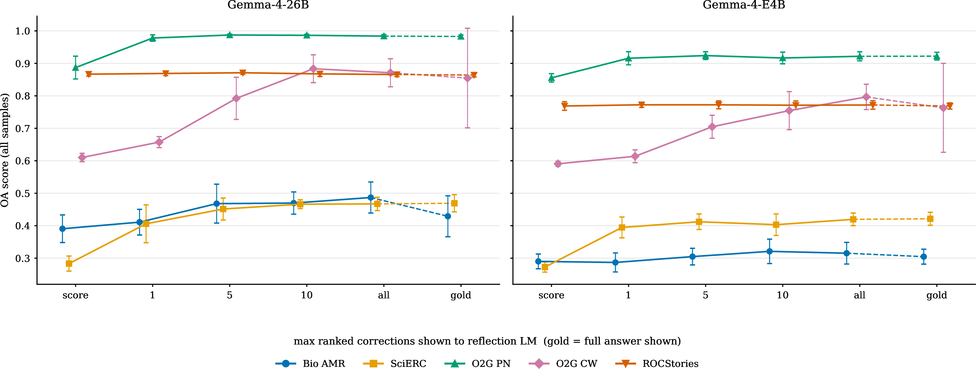
Fig. 9 resolves the contrast into a breadth curve: holding the scalar reward identical, it varies only the number of ranked corrections \(K\) the Object Aligner metric shows the reflection LM. We run the full sweep on the five cells that most sharply discriminate the arms—one plain and one coded Org2Graph variant rather than all four, the two real graph tasks where the structure is most hidden (SciERC, Bio AMR), and ROCStories as the order-axis control. The shape of the curve tracks difficulty: on SciERC and the plain O2G PN, it is steeply concave, a single ranked correction (\(K{=}1\)) already captures most of the gain, whereas on the harder coded O2G CW and the dense Bio AMR, it climbs gradually and most of the gain arrives only by \(K{=}5\)–\(10\). On ROCStories it remains flat throughout, mirroring the null result above.
The gold column appends the full serialized gold answer in the reflection slot—an upper-information control rather than a usable reward signal. It is not a standard input: handed the answer, the reflection LM must itself work out which
parts of its output were wrong, in effect performing LLM-as-judge, and on a more verbose prompt than any deterministic reward would emit. It is also markedly less stable across the seeds on the hardest cells: on the coded O2G CW the gold arm
spans \(\pm0.15\), against \(\pm0.05\) for the capped feedback arms. Its purpose is to bound the value of feedback information from above, and Object Aligner
approaches that bound with little feedback. The default \(K{=}5\) arm already nears gold on most cells, and the uncapped arm meets or exceeds it on the harder ones (Bio AMR, the coded Org2Graph variants,
SciERC). The fact that a short ranked list rivals showing the entire answer is direct evidence the gains come from Object Aligner’s prioritized, localized corrections, not from answer leakage. It also shows that
\(K{=}5\), the cap used throughout our main experiments, was conservative rather than optimal, whereas on the hardest cells, the curve is still climbing at \(K{=}5\), so a larger cap would
have scored higher at the cost of a longer feedback—a trade we did not tune per dataset.
6 Discussion↩︎
The intrinsic study (Section 5.1) shows that each new mechanism is the uniquely correct measurement of its target property: referential alignment (RA) separates damaged graphs from clean ones almost perfectly, where the reference-unaware plain ablation, blind to reference rerouting, does not, and the sequence regime is the only scorer that grades order at all. The extrinsic study asks whether a reward that perceives that property yields a better prompt, and there the answer is conditional. The lesson is that a faithful measurement is not automatically a useful reward: a property-aware reward helps the search only when the property is (i) not already recovered as a by-product of solving the task, and (ii) actionable by the optimizer. The first condition governs when RA (RQ1) and the sequence regime (RQ2) help, and the second condition connects both to deterministic feedback (RQ3).
RQ1. RA helps precisely when node content fails to individuate records, so the score must turn on reference routing rather than on attributes: coded Org2Graph variants, whose identifiers are opaque codes, and Bio AMR, whose dense graphs reuse the same concept symbol across many nodes. Where surface mentions already individuate entities and relations are sparse (SciERC, BioRED), routing is solved before RA is consulted, and the gap becomes small. In the synthetic family, the advantage is monotone in extraction difficulty, widening as readable values become opaque codes, with obfuscation the dominant driver and vocabulary size the smaller one. This is not “RA fails on real data”: RA is the only setting under which a rerouted edge that leaves attributes intact is visible to the score at all, and it pays off extrinsically on Bio AMR, where the same gain carries over in sign to AMR’s own Smatch metric (Appendix 14). What we could not find is a naturally occurring corpus reproducing Org2Graph’s adversarial regime—many property-twin records behind obfuscated ids—under which RA’s payoff is largest; whether such “realistic” data exists in the wild is an open question that normalized relational databases, whose surrogate keys carry no meaning, may answer (Section 9). Several of the datasets that we spot-checked behaved consistently. RA and feedback are also not independent levers: on coded Org2Graph, the RA advantage lives in the feedback arm and vanishes under the scalar score, whereas on Bio AMR, it is the mirror image. The difference is that AMR concepts are genuine, text-derivable semantics, so even plain feedback lists content fixes that repair structure as a by-product, whereas coded identifiers carry no such handle and are recoverable only through RA feedback.
RQ2. The sequence reward is helpful only when the arrangement is the deliverable. On Facts2Order, where items arrive already solved and only their ordering is in question, the sequence reward beats the order-agnostic set reward by a wide margin for every variant. NATURAL PLAN is the contrast: satisfying the flight graph and day budget already forces the city order, which the model then emits as the natural presentation even though the set reward never asks for it, so the sequence reward adds only a marginal gain; ROCStories sits between with a modest gain. Hiding the sort key lowers the absolute score and its seed stability under both rewards alike: a difficulty effect, not a sequence-vs-set one. As with RA, this neutrality is a property of the data, not the extension failing: where correct ordering is inherent to the task, the sequence reward has little extra to teach, yet it remains the only scorer that detects an incorrect order when one occurs. Order sensitivity thus helps as a reward when the output order is itself part of the answer, and is neutral when a correct solution fixes it for free.
RQ3. Deterministic feedback is the most consistently valuable mechanism, and its value scales with how much structure the task hides from a scalar reward. It is decisive where the optimizer must discover something a number
cannot convey—a value-to-code legend, a relation schema, a strict output format: on SciERC the score arm collapses to within noise while feedback recovers a working extractor, and the same drives the gains on coded Org2Graph and Bio AMR. The
feedback-breadth sweep (Fig. 9) rules out the obvious confound: Object Aligner’s short ranked list of localized repairs matches the gold baseline (which appends the
entire answer) on most cells and exceeds it on the hardest ones, while appending less text, direct evidence the gains come from prioritized, localized corrections rather than answer leakage.
The two checks guard against artifacts. Task-model capacity: the two Gemma models bracket a wide range, and capacity shifts magnitudes and absolute scores but not the sign or ordering of any contrast whose \(95\%\) CI excludes zero. Because the reward GEPA optimized was always an Object Aligner schema, we cross-check against a schema-independent native metric on every real-world dataset that carries one (Appendix 14): the native verdict agrees in direction with the headline conclusions, diverging only in informative ways.
For practitioners, the advice is compact and shares one shape: each extension is the correct measurement of its property, and as a reward, each only helped or stayed neutral in our experiments—never a meaningful loss on any Object Aligner-score contrast13—so the practical question is mainly where each pays off most. Enable RA for any (hyper)graph-structured output: it is correct whenever quality is judged up to isomorphism, degrades to plain comparison in the worst case, and pays off most when identifiers are arbitrary and content does not individuate records. Enable the sequence regime whenever the output order is part of correctness—there it never hurts and pays off most when ordering is the deliverable. Finally deterministic feedback is preferred by default: it is the broadest-paying lever, costs no extra model call, and pays off most where the task hides structure from a scalar reward. Unlike an LLM judge, it is reproducible and auditable across any number of rollouts (Section 1).
7 Limitations↩︎
The main limitations fall into two categories: intrinsic properties of the metric and the scope of our empirical evaluation.
Ordinal, not calibrated. The score is ordinal rather than calibrated: \(0\) and \(1\) are anchored and scores are comparable, but an intermediate value such as \(0.51\) is not a literal fraction of correctness—a property Object Aligner shares with many similarity metrics.
Approximate identifier bijection. Referential alignment recovers the gold–candidate identifier bijection by Hungarian assignment on masked attributes, tie-broken by \(1\)-WL color refinement (Section 3.5), which is sound but incomplete approximation to graph isomorphism. On graphs, \(1\)-WL cannot separate, the inferred bijection—and thus the score—can be suboptimal; higher-order \(k\)-WL would tighten it (Section 9).
Self-referential and mutually-referential scopes. Referential alignment resolves scopes in dependency order, so mutually referential scopes (or scope referencing itself) form a cycle with no valid order and fall back to property-only alignment, discarding the reference-value signal. Resolving such cases consistently is a fixed-point problem (akin to collective entity resolution [63]), which we leave for future work. In practice, many such cycles can be sidestepped by reifying the offending references as separate junction (link) table—pure reference-carrier records with no
idScopeof their own, the relational model’s relationship relation [35]—which restores an acyclic scope order, at the cost of treating each edge as an independently matchable record rather than a per-record attribute.Scope of the empirical study. We use a single optimizer (GEPA), a single reflection LM (a strong frontier model, which is best practice), and two task models chosen partly by our available infrastructure; whether the extrinsic findings transfer to other prompt-optimization frameworks or model families is untested, although our partial Qwen robustness check was consistent.
Limited hyperparameter exploration. The cost of the full grid prevented us from sweeping alternative schema-construction strategies, GEPA hyperparameters, and Object Aligner metaparameters (e.g., the feedback list length \(K\)).
Not a benchmark study. Our aim was to demonstrate Object Aligner’s general properties in a prompt-optimization setup, not to set state-of-the-art baselines on the datasets; as a highly configurable metric, Object Aligner may need per-task schema tuning for the best performance.
8 Conclusion↩︎
We presented Object Aligner, an open-source Python library that scores structured LLM outputs against a gold reference deterministically by recursively aligning their JSON trees and awarding partial credit at the granularity a schema declares. Because it is configured entirely through JSON Schema extensions, adapting the Object Aligner to a new task is a matter of annotating a schema rather than writing code, and it drops directly into existing prompt-optimization frameworks such as DSPy, GEPA, and TextGrad as a reproducible, auditable, and model-free alternative to an LLM judge. Its central contribution, referential alignment, makes the score invariant to identifier relabeling, so that cross-referenced records—graphs and hypergraphs—can be compared up to isomorphism, while a complementary order-sensitive sequence regime targets ranking, and the same alignment emits ranked, localized repair suggestions at no extra model cost. Used as the reward inside GEPA across synthetic and real-world datasets, Object Aligner helped or stayed neutral, never a meaningful loss: referential alignment pays off most when identifiers are arbitrary and content fails to individuate records, the sequence regime when the output order is itself the deliverable, and deterministic feedback proved the broadest-paying lever. These findings translate into compact, deployable guidance—enable referential alignment for any (hyper)graph output, the sequence regime whenever order is part of correctness, and prefer deterministic feedback by default—positioning Object Aligner as a practical, drop-in measurement and feedback signal for building and optimizing the structured-output pipelines on which LLM applications increasingly depend.
9 Future Work↩︎
Three directions follow most directly from our findings and the limitations above:
Referential alignment for relational data. The normalized relational databases reproduce Org2Graph’s adversarial regime (Section 6): surrogate keys that carry no content-derived meaning, with foreign keys that are exactly Object Aligner’s
idScope/refstructure, with junction tables as the purest property-twin case. This suggests the application of Object Aligner to text-to-database extraction and database-state diffing, building on the record-linkage lineage (Section 2.1), and collective entity resolution [63].Differentiable surrogates. Object Aligner’s score is derived from a discrete Hungarian assignment; therefore, it can only act as a black-box scalar or textual reward (Section 6). Relaxing the assignment into a soft, entropy-regularized (Sinkhorn-style) matching may yield a differentiable surrogate, opening Object Aligner to gradient-based optimization and end-to-end fine-tuning rather than search alone.
Stronger structural tie-breaking. Replace 1-WL with higher-order \(k\)-dimensional Weisfeiler–Leman to resolve its known blind spots (e.g., one \(6\)-cycle vs.two disjoint \(3\)-cycles), trading the near-linear cost for the combinatorial-in-\(k\) scaling of \(k\)-WL [64].
10 Schema Keyword Reference↩︎
Table ¿tbl:tab:oa-keywords? maps the mathematical notation used in Section 3 to the concrete schema keywords accepted by the implementation. The schema reuses the JSON Schema surface syntax;
standard validation keywords (required, enum, minItems, …) are honored when validating the candidate but do not affect the score. Custom primitive comparators are registered on the aligner and referenced by name.
Table ¿tbl:tab:oa-keywords? lists only the Object Aligner scoring extensions.
@l l l@ Concept / symbol & Keyword & Default
comparator \(\sleaf\) (string) & score & jaro
comparator \(\sleaf\) (number) & score & invdiff
threshold \(\tau\) & threshold & \(0\)
empty-value score (asymmetric) & nullScore & \(0\)
key comparator \(\kappa\) & keyScore & jaro
key threshold \(\tau_K\) & keyThreshold & \(0\)
key weight \(w_K\) & keyImportance & \(0\)
value weight \(w_V\) & valueImportance & \(1\)
per-property weight \(\omega_i\) & valueWeight & \(1\)
order regime & order & fixed
order-agnostic & "align" &
order-sensitive & "fixed" &
prefix weights & prefixWeights & \(1\)
penalize missing (\(n_{\mathrm{miss}}\)) & ignoreMissing & penalize
penalize excess (\(n_{\mathrm{exc}}\)) & ignoreExcess & penalize
prefix importance \(w_p\) & prefixImportance & —
tail importance \(w_r\) & restImportance & —
identifier field & idScope & —
reference field & ref & —
The Object Aligner scoring extensions that appear in the worked schema examples throughout the paper are glossed below: the standard JSON Schema keywords carry their usual meaning. The authoritative specification is the official documentation at https://github.com/aic-factcheck/object_aligner.
score— primitive comparator (exact,jaro,invdiff, …).threshold— minimum primitive similarity to count as a match; below it the pair scores \(0\).order— array regime:"align"(order-agnostic Hungarian matching) or"fixed"(order-sensitive).keyImportance/valueImportance— relative weight of an object’s keys vs.its values in the node score.valueWeight— per-property weight within an object.prefixWeights— per-position weights for theprefixItemsentries.ignoreExcess— do not penalize extra, unmatched candidate elements.idScope— declares a primitive as an identifier within a named scope (enabling referential alignment).ref— declares a primitive as a reference resolved against a namedidScope.
11 Datasets↩︎
This appendix details the real-world datasets used in this study: how each was preprocessed from its source corpus into the JSON output shape we score, the Object Aligner schemas, and the task-native metric we report alongside the Object Aligner score. The synthetic probes (Org2Graph and Facts2Order) are generated rather than preprocessed, and carry no external metric. Because our preprocessing reshapes the original data, the native metric we report sometimes diverges from the dataset’s official metric; we flag each such divergence in the relevant subsection.
11.1 SciERC↩︎
The raw corpus is the sciERC_processed release of [53] (http://nlp.cs.washington.edu/sciIE/). Each raw document carries per-sentence token lists, NER spans (token offsets), mention-pair relations, and coreference clusters. Preprocessing turns each coreference cluster into one entity object
(Fig. 10, middle) whose mentions list holds its de-duplicated surface forms, with the cluster type decided by the majority vote across its spans; NER spans in no cluster become singleton
entities. Mention-pair relations are projected to cluster-level (subject, predicate, object) triples and de-duplicated, and any relation with an endpoint outside a cluster is dropped. Token and character offsets are discarded. One training
document fails to parse, resulting in the \(349/50/100\) native split. The schema scored in the reported run (Fig. 10, bottom) applies Hungarian alignment at two levels: first, to match
entities and then to match the mentions within each matched entity. A coreference cluster that is wrongly split or merged, and therefore costs score.
None
Figure 10: SciERC. Top: the input context (title and abstract). Middle: the gold output—each entity is a coreference cluster, relations reference entities by id. Bottom: the schema as run; the highlighted fragments are exactly what referential alignment adds—idScope on entity ids and ref on relation endpoints; the plain ablation simply omits them,
leaving plain string leaves compared by literal equality..
As the native metric, we use SciERC’s coref-aware entity-level relation F1: predicted entity clusters are aligned to gold, and then relations are scored at the cluster level and micro-averaged, with the symmetric relations
(COMPARE, CONJUNCTION) matching in either argument order. Because preprocessing discards the token offsets and aligns clusters by their surface mention text, this entity-level F1 is not the official span-based SciERC relation F1,
which matches entity boundaries by offset. The same reshaping that defines our task also redefines the metric.
11.2 BioRED↩︎
The raw corpus is the BioRED release of [55] (https://ftp.ncbi.nlm.nih.gov/pub/lu/BioRED/BIORED.zip): \(600\) PubMed titles and abstracts with document-level entity and relation annotations. Preprocessing closely follows SciERC’s (Appendix 11.1): mentions collapse into typed, coreference-merged entities (type by majority vote across the mentions; Fig. 11, middle), relations become de-duplicated
(subject, predicate, object) triples with any out-of-entity endpoint dropped, offsets are discarded, and title and abstract form the input context (Fig. 11, top). Two differences matter. First,
an entity is keyed by its normalized concept id—an Entrez or MeSH accession fixed by the source databases and not derivable from the abstract, whereas SciERC’s entity ids are arbitrary; the model must invent its own, so relations are routed by
referential alignment rather than literal-id matching (Fig. 11, bottom), and a mention tagged with several ids joins every matching entity. Second, the schema scores mention text by
jaro_winkler rather than exact match and up-weights entity type. We draw a seeded \(50/50/100\) train/val/test subsample.
None
Figure 11: BioRED. Top: the input context—title (bold) and abstract. Middle: the gold output—entities are coreference clusters keyed by normalized concept ids (the model invents its own), relations reference them
by id. Bottom: the schema as run; the highlighted idScope/ref fragments are what referential alignment adds over the plain ablation. Mention
text uses jaro_winkler; type is up-weighted..
The native metric mirrors SciERC’s coreference-aware entity-level relation, F1 (Appendix 11.1), but differs in two ways. BioRED relations are directed, so there is no either-order matching (SciERC allows it for its symmetric predicates). The alignment pairs entities by their surface mentions, not their gold concept ids, so the score is not comparable to the official id-keyed metric.
11.3 Bio AMR↩︎
The raw corpus is Release 3.0 of the Bio AMR Corpus [56] (https://amr.isi.edu/download/2018-01-25/amr-release-bio-v3.0.txt): \({\sim}6{,}900\) sentences from cancer-related PubMed articles (each the input context; Fig. 12, top) annotated with Abstract Meaning Representation [57] graphs in PENMAN notation. Preprocessing parses each gold graph into
the JSON output shape in Fig. 12 (middle): a root reference, a list of nodes (each an instance carrying its concept symbol, with constant-valued attributes nested
under their node), and a flat list of relations (source/role/target). The PENMAN variable letters are dropped (they survive only as opaque node ids) so the schema routes relations by referential alignment
over those ids (Fig. 12, bottom). The conversion is lossless: every gold round-trips back to its triple set. A single seeded shuffle with no stratification partitions the corpus into disjoint \(100/100/200\) train/val/test splits.
None
Figure 12: Bio AMR. Top: the input context—a biomedical sentence. Middle: the gold output—a rooted meaning graph of concept nodes, with constant attributes nested under their node and
relations referencing nodes by id; the variable letters are arbitrary, so the model picks its own. Bottom: the schema as run; the highlighted
idScope/ref fragments are exactly what referential alignment adds—the strict ablation omits them, comparing the arbitrary variable letters by literal equality so relation routing collapses. All other leaves are
exact and every array is order-agnostic (AMR is a set of triples)..
As the native metric, we use AMR’s standard metric, Smatch [27]: the best node bijection between the predicted and gold triple sets, with F1 micro-averaged over the corpus. That bijection search is precisely Object Aligner’s referential alignment, so the registered referential schema tracks Smatch by construction.
11.4 NATURAL PLAN↩︎
The raw data are the Trip Planning split of NATURAL PLAN [58] (https://github.com/google-deepmind/natural-plan). Each raw example ships a zero-shot prompt, the target cities and their stay durations as **-delimited fields and a free-text reference plan. Preprocessing keeps the prompt
verbatim as the input context (Fig. 13, top) and builds the gold directly from the cities/durations fields into an itinerary list of {city, days}
objects in the visiting order (Fig. 13, middle). The NATURAL PLAN is evaluation-only (no native train split), so we keep train and val small (\(100\) each) and a \(200\)-example test split, all difficulty-stratified by the number of cities (\(3\)–\(10\)). The schema used in the reported run (Fig. 13, bottom) aligns the itinerary by position, so producing the correct stays in the wrong order loses score.
None
Figure 13: NATURAL PLAN (Trip Planning). Top: the input context—the zero-shot trip problem, stating the day budget, the per-city stays and meeting windows, and the available direct flights. Middle: the gold
output—an ordered itinerary of {city, days} stays, taken from the released target fields. Bottom: the schema as run; the highlighted value is the
sequence arm—order set to "fixed", which aligns the itinerary positionally so a scrambled sequence is penalized—while the set ablation replaces it with "align" (order-blind Hungarian matching).
city is matched exactly (it is copied from the prompt) and days by the graded inverse-difference comparator..
As the native metric we use NATURAL PLAN’s official metric, the binary per-example exact-match solve rate: a plan solves the instance iff its (city, days) itinerary reproduces the gold stay for stay, in order, averaged over the split.
11.5 ROCStories↩︎
The raw data are the ROCStories corpus [59], taken from https://huggingface.co/datasets/mintujupally/ROCStories. Each story is split into sentences on sentence-ending punctuation, and only stories that are segmented into exactly five sentences are retained. For each story, we draw a random
non-identity permutation and present the sentences in that scrambled order—labeled \(1..N\) in the input context (Fig. 14, top)—and recorded as gold the permutation of
those labels that restores the original reading order (Fig. 14, middle). The splits are mutually disjoint: \(100/100\) train/val and a \(200\)-example test. The schema scored in the reported run (Fig. 14, bottom) aligns the indices list positionally.
None
Figure 14: ROCStories (sentence ordering). Top: the input context—the five story sentences presented in scrambled order and labelled \(1..N\). Middle: the gold output—the
indices permutation of those labels that restores the original reading order. Bottom: the schema as run; the highlighted value is the sequence
arm—order set to "fixed", which aligns the indices list positionally so a scrambled order is penalized—while the set ablation replaces it with "align" (order-blind Hungarian matching). The data
key is the neutral indices (not order), so neither schema nor prompt reveals that the task is a reordering..
As the native metric, we use the standard sentence-ordering Perfect-Match Ratio (PMR) [65], the fraction of stories whose predicted order reproduces the gold permutation exactly, alongside Kendall’s \(\tau\) as a graded view of partial order [65]. Because the predicted bag of labels is always exactly the gold bag, the order-blind set arm of the Object Aligner reward scores \(\approx\!1.0\) regardless of sequence, so the entire sequence-vs-set gap is attributable to order alone.
12 Intrinsic Validation↩︎
This appendix collects additional material for the intrinsic validation of Section 5.1.
12.0.0.1 A worked referential-alignment instance.
Fig. 15 shows the unit of the invariance probe of Section 5.1: a small Org2Graph instance and its relabel-only candidate. Every identifier differs, yet referential alignment
recovers the bijection \(\pi\) and scores \(1.0\), while the plain ablation compares the renumbered identifiers by value and matches no reference. The two
Milo/scientist records show why this is nontrivial: tied in every attribute, they are separable only by structure—twin A is the source of the reports_to and knows edges, twin B only a
target—which the structural tie-break of Section 3.5 uses to pin the bijection.
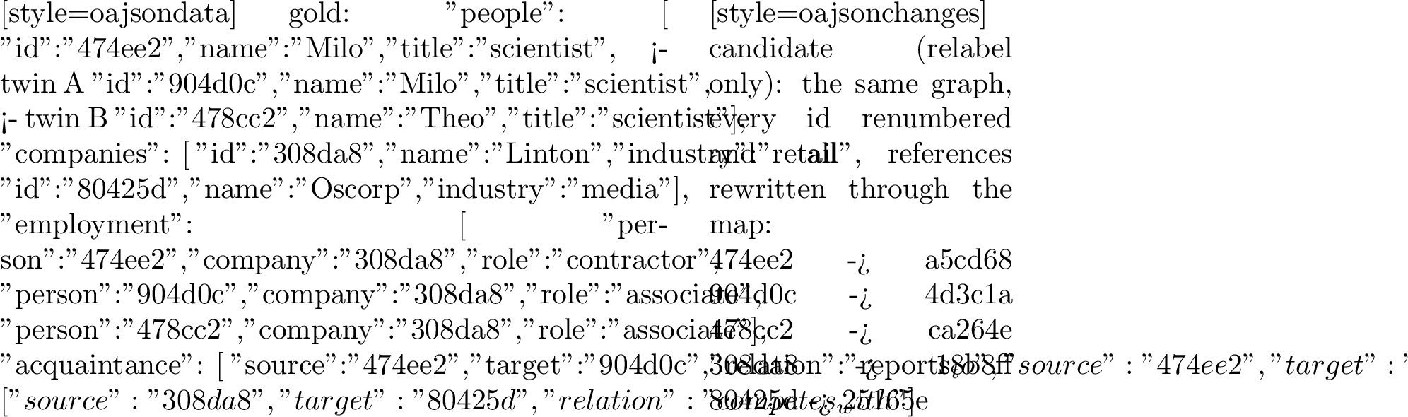
12.0.0.2 RA Data generation.
Algorithms 16 and 17 provide the exact procedures for the two RA experiments described in Section 5.1. In this appendix, the emit appends one gold/candidate pair, with its family and magnitude tags, to the generated dataset. Every gold draws its parameters independently via SampleParams (Algorithm 16, lines 2–4), so both experiments cover the same distribution of graphs. They share three additional primitives. SampleGold draws an Org2Graph instance with readable (un-obfuscated) categorical values and the narrow \(6/6/6/3/3\) vocabulary (Section 4.1) at the requested sizes and edge densities; MakeTwins turns a fraction \(t\) of each scope’s records into property-twins; Relabel reassigns every record a fresh identifier, disjoint from the gold’s, and rewrites all references accordingly. In Algorithm 17, each \((o,k)\) candidate is built independently from the gold. The six edit operations \(\mathcal{O}\) are as follows:
categorical relabel — pick a uniformly random categorical leaf (a person’s title, a company’s industry, an employment role, or an edge relation) and set it to a different code from the same codebook (Section 4.1);
reference rerouting — pick a random edge endpoint whose scope holds \({\ge}2\) records and rewire it to a different record’s id;
record deletion — pick a random scope still holding \({\ge}2\) records, delete a random record together with every incident edge;
edge deletion — delete a uniformly random edge;
record insertion — insert a fresh record with a new id and sampled attributes (a new person also receives an employment edge to a random company);
edge insertion — add a new acquaintance (two distinct random people) or partnership (two distinct random companies) edge with a sampled relation.
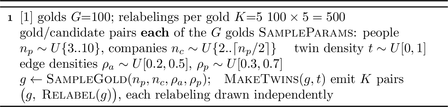

12.0.0.3 RA per-operation effects.
Table 5 quantifies the per-operation sensitivity behind Fig. 6: the Spearman correlation of score with the number of applications \(k\) of a single edit.
| Operation | RA | plain |
|---|---|---|
| categorical relabel | \(-0.784\) | \(-0.460\) |
| reference rerouting | \(\mathbf{-0.660}\) | \(\mathbf{-0.011}\) |
| record deletion | \(-0.818\) | \(-0.776\) |
| edge deletion | \(-0.771\) | \(-0.627\) |
| record insertion | \(-0.888\) | \(-0.779\) |
| edge insertion | \(-0.667\) | \(-0.604\) |
6pt
12.0.0.4 A worked Facts2Order instance.
Fig. 18 shows a hidden-key Facts2Order instance (\(N{=}4\), integer key): the designated sort key (weight) is buried among per-item numeric decoy clauses on other attributes (price, length) whose values are unconstrained, their order shuffled per item, so the key is never identifiable as the lone number. Only the weights are drawn distinct, fixing a unique gold order; the optimizer must discover from Object Aligner feedback that weight—not price or length—is the sort field. (The intrinsic study described in Section 5.1 ignores these surface sentences and scores the index permutations directly; cf.Fig. 7.)
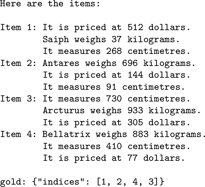
12.0.0.5 Order data generation.
Algorithm 19 provides the exact procedure for the Facts2Order corruption pairs described in Section 5.1, which yields \(4639\) pairs at the sampled sizes (the per-gold count increases with \(N\)). Every gold sample draws its parameters via SampleParams (Section 4.2), and SampleGold returns the unique permutation of \(1..N\) that sorts the items, which the study scores directly (ignoring surface sentences). Each gold is corrupted once per family into a candidate, tagged by its realized Kendall distance \(d\), and all draws use per-gold seeds for reproducibility. Each family targets a distinct failure mode:
adjacent transpositions (\(k{=}1..N{-}1\) swaps) — walking \(d\) up in approximately unit steps to trace the partial-credit curve; \(d\) is recomputed per candidate, so a fixed \(k\) spreads over a small range as shown in Table 2;
block reversal / block move — reverse, or cut and reinsert, one contiguous block (length \({\ge}2\)): non-local disorder — large per-item displacement that a single local swap cannot produce;
deletion / insertion (drop, or inject duplicate, labels) — change the candidate length, exercising the gap-aligned DP denominator and excess penalty. Unlike the reorderings, these alter the label bag, so the order-agnostic baseline reacts to them but not to pure order.
The uncorrupted gold paired with itself is the none (\(d{=}0\)) reference row in Table 2. Corruptions that reproduce the gold are resampled, because AdjTranspose and BlockMove can compose to the identity. Across the generated pairs, \(d\) is concentrated near the gold: of the \(2864\) length-preserving pairs, it ranges \(0\)–\(55\) with a median of \(2\) (the dense low-\(d\) region comes from the adjacent-transposition dose, the sparse tail from the block families), while the \(1775\) length-changing deletion/insertion pairs leave \(d\) undefined.
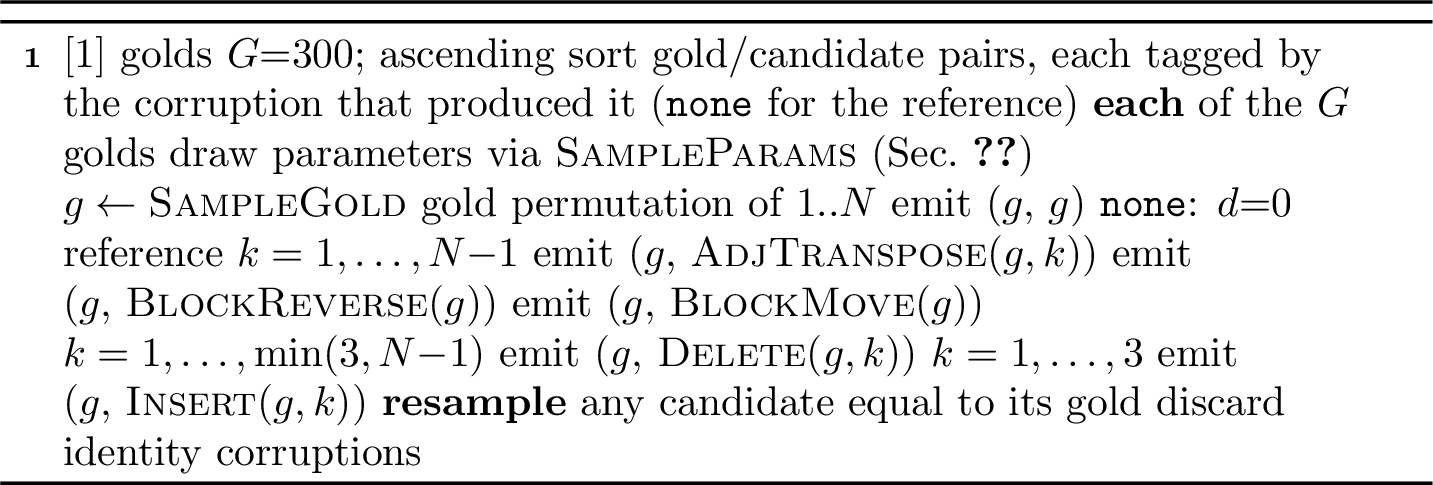
12.0.0.6 Order-sensitivity curves.
Fig. 20 shows the curve view of Table 2, showing the full trend of the table samples at a few points. One feature deserves comment: on pure reorderings Kendall \(\tau\) sits above the sequence score at every distance. This is a difference of scale, not of sensitivity—\(\tau\) rescales the inversion count, while the sequence alignment pays per displaced item—so the two are comparable in trend, but not in level.

13 System Prompts↩︎
This appendix lists the initial candidate system prompt used to seed GEPA for every dataset. As discussed in the protocol of Section 5 (paragraph “Protocol”), each seed prompt is deliberately minimal: beyond a one-line statement of the task and the required JSON output shape, it gives no guidance on how to produce the prediction. The task model is told what kind of object to emit, but not the rules, edge cases, or step-by-step procedure for deriving it from the input, so GEPA must recover that mapping purely from the Object Aligner’s scalar score and—in the feedback arm—its textual feedback. This isolates the question of whether the metric supplies sufficient optimization “gradient” to drive the search from a near-empty starting point. The prompts below are reproduced verbatim.
13.0.0.1 Org2Graph.
You extract a graph of people and companies from a short English paragraph.

Output a SINGLE JSON object with exactly these five top-level keys:
  "people":       a list of {"id": <string>, "name": <string>, "title": <string>} objects.
  "companies":    a list of {"id": <string>, "name": <string>, "industry": <string>} objects.
  "employment":   a list of {"person": <person-id>, "company": <company-id>, "role": <string>} objects.
  "acquaintance": a list of {"source": <person-id>, "target": <person-id>, "relation": <string>} objects.
  "partnership":  a list of {"source": <company-id>, "target": <company-id>, "relation": <string>} objects.

Use short, stable ids of your own choosing (e.g. "p0", "p1", "c0", "c1"); the
exact id strings do not matter as long as each person / company has one
consistent id and every edge references ids defined in "people" / "companies".
"person" and acquaintance source/target are person-ids; "company" and
partnership source/target are company-ids.

Emit JSON only — no commentary, no markdown fences.
13.0.0.2 Facts2Order.
Output a SINGLE JSON object with exactly one top-level key:
  "indices": a list of integers — a permutation of 1..N, where N is the number
             of input items. Example: {"indices": [3, 1, 4, 2]}.

Emit JSON only — no commentary, no markdown fences.
13.0.0.3 SciERC.
You extract a scientific knowledge graph from an AI-paper abstract.

Output a SINGLE JSON object with exactly these two top-level keys:
  "entities":  a list of {"id": <string>, "type": <string>, "mentions": [{"text": <string>}, ...]} objects.
  "relations": a list of {"subject": <entity-id>, "predicate": <string>, "object": <entity-id>} objects.

Use short, stable ids of your own choosing (e.g. "e0", "e1"); the exact id
strings do not matter as long as each entity has one consistent id and every
relation's "subject" / "object" references ids defined in "entities". Each
entity carries all of its surface mentions in its "mentions" list.

Emit JSON only — no commentary, no markdown fences.
13.0.0.4 BioRED.
You extract a biomedical relation graph from a PubMed title and abstract.

Output a SINGLE JSON object with exactly these two top-level keys:
  "entities":  a list of {"id": <string>, "type": <string>, "mentions": [{"text": <string>}, ...]} objects.
  "relations": a list of {"subject": <entity-id>, "predicate": <string>, "object": <entity-id>} objects.

Use short, stable ids of your own choosing (e.g. "e0", "e1"); the exact id
strings do not matter as long as each entity has one consistent id and every
relation's "subject" / "object" references ids defined in "entities". Each
entity carries all of its surface mentions in its "mentions" list.

Emit JSON only — no commentary, no markdown fences.
13.0.0.5 Bio AMR.
You convert an English sentence into an Abstract Meaning Representation (AMR) graph.

Output a SINGLE JSON object with exactly these top-level keys:
  "root":      the id of the top node.
  "nodes":     a list of {"id": <string>, "concept": <string>, "attributes": [{"role": <string>, "value": <string>}, ...]} objects.
  "relations": a list of {"source": <node-id>, "role": <string>, "target": <node-id>} objects.

Use short, stable ids of your own choosing (e.g. "n0", "n1"); the exact id strings
do not matter as long as every relation and the root reference ids defined in "nodes".

Emit JSON only — no commentary, no markdown fences.
13.0.0.6 NATURAL PLAN (Trip Planning).
You are an expert trip planner. The user message states how many days the trip
lasts, which cities to visit and for how long, any meeting/event day-window
constraints, and the available direct flights between cities. Find an itinerary
that satisfies every constraint, taking only the listed direct flights.

Output a SINGLE JSON object with exactly one top-level key:
  "itinerary": a list of {"city": <string>, "days": <integer>} objects, in the
               order the cities are visited.

Emit JSON only — no commentary, no markdown fences.
13.0.0.7 ROCStories.
Output a SINGLE JSON object with exactly one top-level key:
  "indices": a list of integers — a permutation of 1..N, where N is the number
             of input sentences. Example: {"indices": [3, 1, 4, 2, 5]}.

Emit JSON only — no commentary, no markdown fences.
14 Native-Metric Results↩︎

Where a real-world task carries a standard metric of its own we report it here as a fully schema-independent cross-check on the OA-score conclusions of Section 5. Because GEPA always optimized an Object Aligner schema, a metric that lies outside that schema (and so is unaffected by any ablation) provides an independent external check. On all three axes, the native verdict agrees with the headline directions of Fig. 8 (Fig. 21): sequence beats set wherever order matters, feedback beats score everywhere, and on Bio AMR, the gain from referential alignment over the plain schema, seen in the Object Aligner score under the score reward, carries over in sign to Smatch (\(+0.030\), Gemma-4-26B), though within seed noise (\(95\%\) bootstrap CI \([-0.03, +0.09]\)). One qualitative difference is worth flagging: on SciERC and BioRED the score arm collapses to exactly \(0.000\) relation F1 (both RA and plain), even though its Object Aligner graded score does not: relation F1 credits only relations whose subject, predicate, and object all match the gold; a near-miss earns nothing. Labelling the right pair of entities USED-FOR, where the gold
says PART-OF, for instance, scores \(0\) even though two of its three fields are correct. The model become accurate enough to register any F1 only under the feedback reward. Elsewhere the native and Object Aligner-score gaps differ only in magnitude, agreeing in sign and ordering.
These native metrics are not all standard leaderboard tasks. For SciERC and BioRED, there are no published number lines up with our setup: the relation F1 we report is simply the conventional metric for relation extraction on data of that kind, adopted here as a schema-independent alternative to the Object Aligner score rather than to match an external baseline. The remaining three—Bio AMR, NATURAL PLAN, and ROCStories—do have published reference points, which we quote below; even there the comparison is loose (splits, models, and task framing all differ), so we cite them only to locate the scale of each metric, not as head-to-head results.
On Bio AMR, the prompted model sits far below the supervised state of the art. Our best (Gemma-4-26B, feedback RA) reaches \(\approx\!0.40\) Smatch F1, whereas purpose-built AMR parsers report low-to-mid-\(0.80\)s on the Bio test set—StructBART with Maximum-Bayes-Smatch ensemble distillation [66] at \(\approx\!0.81\). These parsers are fine-tuned on AMR (including the Bio training portion) and emit PENMAN on the corpus’s standard split. We score a general-purpose open model emitting a JSON graph under a GEPA-optimized prompt on a seeded \(200\)-example subsample. The gap reflects supervised, in-domain training versus none, not a weakness of the Object Aligner reward.
On NATURAL PLAN (Trip Planning), whose official metric is the exact-match (EM) solve rate, our best Gemma-4-26B result reaches \(\approx\!0.63\) EM—above the benchmark’s figures (GPT-4 \(31.1\%\), the strongest model Gemini 1.5 Pro \(34.8\%\)) [58]. The lead is not evidence of better planning: those are 2024-era models (although frontier at that time) evaluated \(5\)-shot over the full \(1600\)-example set, whereas we score a newer-generation open model on a \(200\)-example, city-count-stratified split with a GEPA-optimized prompt, so the gap reflects the changed evaluation setup (a different-generation model and an optimized prompt) not planning ability.
On ROCStories, the prompted model again sits somewhat below the supervised state-of-the-art. Our Gemma-4-26B sequence arm scores \(\approx\!0.65\) PMR and \(\approx\!0.87\) Kendall’s \(\tau\), whereas Re-BART [65], fine-tuned end-to-end to order the sentences, reports \(0.82\) PMR and \(0.94\) \(\tau\) (full corpus, \(80{:}10{:}10\) split, \(\approx\!9.8\)K test stories). The gap is smaller on the graded \(\tau\) than on exact-match PMR, as expected when a prompted model recovers the rough order but rarely the exact permutation.
Acknowledgment↩︎
This work was supported by the Ministry of Education, Youth and Sports of the Czech Republic through the e-INFRA CZ (ID:90254). The author thanks Herbert Ullrich for proof-reading the manuscript and for his valuable suggestions.
During the preparation of this work, the author used generative AI tools, predominantly the Anthropic Claude Code (mainly Opus models) and secondarily ChatGPT (OpenAI GPT-5). The core of the Object Aligner library was written manually and later refactored with AI assistance. Several extensions, the test and experimental-suite code, and supporting utilities were drafted with AI, which was also used for code review to identify errors. For the manuscript, AI was used for grammar correction and extensively for rephrasing. Some passages, mainly in the related-work and dataset-description sections, were drafted by AI from detailed bullet outlines written by the author, and all figures and tables were produced by AI-generated scripts that construct them from the actual computed results. AI was also used to assist in researching related topics. The author reviewed, verified, and edited all AI-assisted content and takes full responsibility for the content of this publication.
Jan Drchal is an assistant professor at the Faculty of Electrical Engineering (FEE), Czech Technical University in Prague (CTU). He received the Ing. (2006) and Ph.D. (2013) degrees in electronics and computer science from CTU. His doctoral dissertation focused on evolutionary optimization of artificial neural networks. He is a member of the Artificial Intelligence Center (http://aic.fel.cvut.cz).
Following his doctoral work, he worked mostly on machine learning applications in transportation and robotics. Since 2021, his research has centered on natural language processing, with application domains including AI-assisted journalism, automated fact-checking, information extraction, and prompt optimization.
References↩︎
gpt-5-2025-08-07 snapshot. Accessed: 2026-06-28“GPT-5 system card.” https://cdn.openai.com/gpt-5-system-card.pdf, 2025.gemma-4-26B-A4B-it and gemma-4-E4B-it instruction-tuned variants. Accessed:
2026-06-28“Gemma 4 model card.” https://ai.google.dev/gemma/docs/core/model_card_4, 2026.J. Drchal is with the Artificial Intelligence Center, Faculty of Electrical Engineering, Czech Technical University in Prague, Czech Republic (e-mail: drchajan@fel.cvut.cz).↩︎
This work was created with the state support of the Technology Agency of the Czech Republic within the Sigma Programme, Project No. TQ01000100.↩︎
Preprint. This is a submitted version of a manuscript under review at IEEE Access; it has not been peer reviewed.↩︎
Following common usage in the evaluation literature, we use the terms “score” and “metric” interchangeably, even though Object Aligner is not a metric in the strict mathematical sense.↩︎
https://github.com/aic-factcheck/prompt_opt, committed 2024-12-20.↩︎
The code for all experiments is available at https://github.com/aic-factcheck/object_aligner_paper, ensuring the reproducibility.↩︎
User-defined primitive type comparators, such as semantic embedding-based scores, may break determinism.↩︎
Scalars compared by a graded similarity rather than exact equality (e.g., Jaro string distance or inverse numeric difference), whose partial scores have no place in WL’s exact-equality color refinement.↩︎
As an additional robustness check, we ran Qwen3.5-35B-A3B and Qwen3.5-9B [62] as task models on a subset of datasets. The qualitative conclusions were unchanged.↩︎
The lone exception is the BioRED Gemma-4-26B score arm: \(+0.026\) (CI \([+0.012,+0.048]\)), a small gain at the edge of detectability.↩︎
Although small, the Gemma-4-26B gap is statistically detectable: \(+0.025\) (\(95\%\) CI \([+0.008,+0.045]\)) under the score reward and \(+0.023\) (\(95\%\) CI \([+0.005,+0.046]\)) under feedback, both excluding zero; on Gemma-4-E4B it is indistinguishable from zero.↩︎
The one exception is negligible: on the ROCStories set arm, feedback trails score by \(-0.004\) (\(95\%\) bootstrap CI \([-0.006, -0.000]\)).↩︎