Regularized Variational and Spectral Log-Density-Ratio Estimation
in the Gaussian Location Model
July 02, 2026
Abstract
We study ridge-regularized log-density-ratio estimation in the Gaussian location model with a common covariance matrix. By affine invariance, the model is written as \(q\sim\mathcal{N}(0,I)\), \(p\sim\mathcal{N}(\Delta,I)\), with linear features, where \(\Delta \in \mathbb{R}^m\) and the signal strength \(s=\|\Delta\|^2\) is fixed. The variational estimator is the empirical Kullback-Leibler (KL) log-normalized fit with a squared \(\ell_2\)-penalty on its nonconstant coefficient, and the spectral estimator recently introduced in [1] replaces a single variational problem by a continuum of ridge-regularized least-squares problems.
We derive high-dimensional deterministic asymptotic equivalents when the numbers of observations and dimension tend to infinity with fixed ratios. The regularized variational limit is characterized by a scalar entropy minimization problem derived from the convex-Gaussian-min-max theorem (CGMT), while the regularized spectral limit follows from deterministic equivalents for resolvents of weighted sums of two independent Gaussian sample covariance matrices. We use these formulas to compare population risks, with experiments focused on fixed-signal aspect-ratio sweeps and optimized regularization. Our conclusion is that with many observations, under the criteria and asymptotic regimes analyzed here, the well-specified variational estimator has the smaller risk, while with fewer observations, the spectral estimator is favored because its covariance-based construction has lower variance. We also study how a nuclear penalty can be used and partially analyzed to perform feature learning.
1 Introduction↩︎
Estimating a log-density ratio from two samples is a central primitive in machine learning and data science, with applications to covariate-shift correction, two-sample testing, importance weighting, likelihood-free inference, and variational estimation of divergences [2]–[5]. A common approach is to use a variational representation of the Kullback–Leibler (KL) divergence, fit a real-valued potential \(v\) from samples of \(p\) and \(q\), and interpret \(v\) as an estimate of \(\log(dp/dq)\) [5]–[7]. Without regularization this approach is exposed to the variance of empirical exponential normalization: a few sample points from \(q\) can dominate the “log-sum-exp” term, and in high dimension, the empirical objective can even be unbounded, like in logistic regression [8], [9]. Ridge regularization is the standard remedy, going back to the classical ridge regression literature [10]; it makes the optimization problem finite and stable, but it also introduces shrinkage bias. The central question of this paper is to understand how the performance of regularized estimators depends on signal strength, aspect ratios (ratios between dimension and number of observations), and the ridge parameters.
Our main goal is to understand the performance of the recent spectral framework for relative density estimation [1], which represents the KL divergence as a mixture of weighted chi-square divergences. This turns the estimation of a log-density potential into a family of least-squares problems indexed by a mixture parameter \(\rho\in[0,1]\). The integral with respect to \(\rho\) can be carried out in closed form using a generalized eigenvalue decomposition of second-order moments; this spectral construction has thus closed-form computation through empirical first and second moments, with a ridge penalty needed to stabilize estimation. The reformulation as a continuum of least-squares problems immediately brings to bear the large literature on algorithms and analyses for least-squares regression to control estimation variance, but this closed-form estimator comes at a cost of potential additional bias.
We compare the ridge-regularized variational and spectral estimators in a simple Gaussian location model. By affine invariance and whitening, it is enough to consider, in dimension \(m\), \[q\sim\mathcal{N}(0,I),\qquad p\sim\mathcal{N}(\Delta,I),\] with linear models (with unregularized intercept).1 We consider \(n_p\) i.i.d. samples from \(p\), and \(n_q\) from \(q\), in the high-dimensional proportional regime, that is, with the following dimension-to-sample ratios, which will be referred to as aspect ratios from now on, \[\frac{m}{n_p}\to\alpha_p\in[0,\infty), \qquad \frac{m}{n_q}\to\alpha_q\in[0,\infty).\] The signal strength \(s=\|\Delta\|^2\) is fixed in the main asymptotic statements and in our experiments. This model is deliberately favorable to the variational estimator because the true log-density ratio is affine. The spectral estimator is, however, not exactly well-specified, but it can reduce estimation variance by replacing empirical exponential normalization with covariance-based least squares. The goal of this paper is precisely to determine when, in this simple model, this variance reduction translates into smaller population risk.
1.0.0.1 Contributions.
The first contribution of this paper is a set of finite-sample identities for the regularized and unregularized estimators, presented in Section [sec:finite], complemented by a population analysis in Section [sec:pop-bench] to understand the shrinkage bias due to regularization. The second and main contribution is a high-dimensional fixed-signal analysis presented in Section [sec:hd]: The variational limit is a scalar entropy minimization problem obtained from CGMT. The spectral limit is a deterministic equivalent for ridge-regularized weighted sums of two Wishart matrices. The third contribution is a risk comparison under three different natural criteria for unregularized and regularized estimation, which we perform in Section [sec:weak] for small \(\alpha_p\) and \(\alpha_q\) with further asymptotic expansions, and in Section [sec:comparison] by plotting deterministic asymptotic limits in the \((\alpha_p,\alpha_q)\)-plane, highlighting that the variational estimator outperforms the spectral estimator when \(\alpha_p\) and \(\alpha_q\) are small (many observations), but underperforms when these two parameters grow. In Section [sec:experiments], we illustrate the asymptotic limit by comparing empirical estimates with their asymptotic equivalents. Finally, in Appendix 16, we also study how a nuclear penalty can be used and partially analyzed to perform feature learning (for simplicity, we only consider discrete measures on \(\rho\) instead of continuous measures needed for the KL divergence).
1.1 Related work↩︎
1.1.0.1 Direct density-ratio estimation.
In this paper, we compare only two estimators for log-density ratios, a natural one based on a classical variational representation of the KL divergence [5], and the recently introduced spectral estimators [1]. Other estimators could be considered as well, see, e.g., [2]–[4], [11], [12].
1.1.0.2 Asymptotic analysis of maximum-likelihood estimators.
Our analysis of the variational estimator shares many features with the analysis of maximum-likelihood estimators, such as logistic regression, with similar potential unboundedness when not regularized [8], [9], [13]; we use similar tools such as the convex-Gaussian-min-max theorem (CGMT) [14].
1.1.0.3 Random matrix theory.
Our analysis for the spectral estimator essentially corresponds to doing a separate analysis for each \(\rho \in [0,1]\) and a single regularized least-squares problem, for which there exists a significant literature, which we reuse here [15], [16]. Closest in goal are analyses of ridge regression and regularized discriminant analysis, where random-matrix methods yield explicit limiting prediction-risk formulas [17]. Our setting differs in that the spectral estimator requires a continuum of \(\rho\)-weighted covariance resolvents from two independent samples, with cross-resolvent quantities entering the final risk formulas. We use degree-of-freedom quantities in the spirit of [18], [19].
2 Problem setup↩︎
This section describes in detail the Gaussian model, the two estimators, and the criteria that we consider in this paper, without imposing proportional-asymptotic assumptions on \(m,n_p,n_q\). The KL variational identities are the Donsker-Varadhan and Fenchel representations of KL [5], [6], and the spectral construction follows the spectral relative-density framework of [1].
2.1 Gaussian model and samples↩︎
We consider the Gaussian model \[q\sim \mathcal{N}(0,I),\qquad p\sim\mathcal{N}(\Delta,I),\] with \(\Delta\in\mathbb{R}^m\) and \(s = \| \Delta \|^2\). The true normalized log-density ratio is \[v_\ast(x)= \log \frac{dp}{dq}(x) = \frac{1}{2} \| x\|^2 - \frac{1}{2} \| x - \Delta\|^2 = \Delta^\top x-\frac{s}{2}, \qquadwith\qquad D(p\|q)=\frac{s}{2}.\] We observe independent samples \[x_i\sim p, \quad i=1,\ldots,n_p, \qquad y_j\sim q, \quad j=1,\ldots,n_q.\] We can then write the empirical means and their difference as \[\hat{\mu}_p=\frac{1}{n_p}\sum_{i=1}^{n_p}x_i, \qquad \hat{\mu}_q=\frac{1}{n_q}\sum_{j=1}^{n_q}y_j, \qquad \hat{\Delta}=\hat{\mu}_p-\hat{\mu}_q.\] The centered sample covariances, normalized by \(1/n_p\) and \(1/n_q\), are \[\hat{C}_p=\frac{1}{n_p}\sum_{i=1}^{n_p}(x_i-\hat{\mu}_p)(x_i-\hat{\mu}_p)^\top, \qquad \hat{C}_q=\frac{1}{n_q}\sum_{j=1}^{n_q}(y_j-\hat{\mu}_q)(y_j-\hat{\mu}_q)^\top.\]
2.2 Variational estimator and its ridge-regularized version↩︎
The variational estimator is the KL special case of the convex risk-minimization framework of [5], which states, for general probability distributions,2 \[D(p\|q) = \sup_{v: \mathbb{R}^m \to \mathbb{R}} \mathbb{E}_p[v(x)]-\mathbb{E}_q[e^{v(y)}-1].\] This leads, for a measurable function \(v\), to the population Fenchel score for KL: \[\mathcal{K}(v)=\mathbb{E}_p[v(x)]-\mathbb{E}_q[e^{v(y)}-1].\] If we consider a potential with an additional intercept, as \(\tilde{v} (x)=v(x)+c\), then \(\mathcal{K}(\tilde{v} )= \mathbb{E}_p[v(x)]+c+1-e^c\mathbb{E}_q [e^{v(y)}].\) For fixed \(v\), the intercept is optimized in closed form as \(c_\ast =-\log\mathbb{E}_q[ e^{v(y)}].\) Substitution gives the log-normalized population objective \[\mathcal{J}(v)= \mathbb{E}_p[v(x)]-\log\big( \mathbb{E}_q [e^{v(y)}] \big).\] The empirical version replaces \(\mathbb{E}_p\) and \(\mathbb{E}_q\) by sample averages, and we now consider a linear model \(v(x) = \theta^\top x\). Thus, over these affine potentials, the empirical intercept for a fixed \(\theta\) is \[\hat{c}(\theta)=-\log\bigg(\frac{1}{n_q}\sum_{j=1}^{n_q}\exp(\theta^\top y_j)\bigg),\] and the optimized empirical criterion is the log-normalized objective in \(\theta\), on which we add a ridge penalty (only on the linear term, because the intercept has already been optimized by normalization), leading to, for \(\tau >0\), \[\widehat{\mathcal{J}}(\theta) =\theta^\top\hat{\mu}_p -\log\bigg(\frac{1}{n_q}\sum_{j=1}^{n_q}\exp(\theta^\top y_j)\bigg) -\frac{\tau}{2}\|\theta\|^2 . \label{eq:Jhat-ridge}\tag{1}\] The ridge estimator is \(\hat{\theta}\in\arg\max_{\theta\in\mathbb{R}^m}\widehat{\mathcal{J}}(\theta).\) For every sample and every \(\tau>0\), the objective is strongly concave, hence the maximizer exists and is unique.
For criterion \(\mathcal{K}\), which is sensitive to additive constants, we use the empirically normalized representative \[\hat{v}_{{\rm var}}(x)=\hat{\theta}^\top x+\hat{c}, \qquadwith\hat{c} =-\log\bigg(\frac{1}{n_q}\sum_{j=1}^{n_q}\exp(\hat{\theta}^\top y_j)\bigg).\]
The unregularized estimator is obtained by dropping the last term in 1 . Unlike the ridge estimator, the unregularized objective can be unbounded; Proposition 4 in Section [sec:zeroridge] gives the exact convex-hull condition for finite value and finite attainment.
2.2.0.1 Estimation algorithm.
The objective function in Eq. (1 ) is smooth and strongly concave if \(\tau>0\), so damped Newton [20], trust-region Newton, or L-BFGS with backtracking line search (as used in the experiments) are globally well-behaved choices [21], [22].
2.3 Spectral estimator↩︎
The spectral estimator of [1] starts from an equivalent two-potential variational formulation [23] \[\label{eq:DKL2} D(p\|q) = \sup_{v,w: \mathbb{R}^m \to \mathbb{R}} \mathbb{E}_p [ v(x)]+\mathbb{E}_q [w(y)],such that\forall y \in \mathbb{R}^m, \;w(y)\leqslant 1-e^{v(y)}.\tag{2}\] The optimum of the associated variational problem is attained by \(v_\ast=\log(dp/dq)\) and \(w_\ast=1-dp/dq.\) We will estimate these two potentials through a continuum of least-squares problems.
The key contribution of [1] is to represent the KL divergence as an integral of weighted chi-square divergences as \[\begin{align} \notag &\!\! \!\! & D(p\|q) \\ \notag &\!\!\!\!\! = \!\!\!\!\!& \int_{\mathbb{R}^m} \int_0^1 \frac{ (\frac{dp}{dq}(x) - 1)^2}{\rho \frac{dp}{dq}(x) + 1-\rho} (1-\rho)d \rho dq(x) \\ \label{eq:AAAA}& \!\!\!\!\!= \!\!\!\!\! & \int_0^1 \bigg[ \sup_{u(\rho,\cdot):\mathbb{R}^m\to \mathbb{R}}\; \int_{\mathbb{R}^m} \Big[ u(\rho,x) \Big( \frac{dp}{dq}(x) - 1 \Big) - \frac{u(\rho,x)^2}{2} \Big( \rho \frac{dp}{dq}(x) + 1-\rho\Big) \Big] dq(x) \bigg] 2 (1-\rho) d\rho \\ \notag&\!\!\!\!\! = \!\!\!\!\!& \int_0^1 \bigg[ \sup_{u(\rho,\cdot):\mathbb{R}^m \to \mathbb{R}}\; \int_{\mathbb{R}^m} \Big[ u(\rho,x) - \frac{\rho}{2} u(\rho,x)^2 \Big] dp(x) + \int_{\mathbb{R}^m} \Big[ - u(\rho,x) - \frac{1-\rho}{2} u(\rho,x)^2 \Big] dq(x) \bigg] 2 (1-\rho) d\rho, \end{align}\tag{3}\] with the integrand having its own variational formulation through a function \(u(\rho,\cdot): \mathbb{R}^m \to \mathbb{R}\) for \(\rho\in[0,1]\). The population optimal variational function for each \(\rho \in [0,1]\) is \[u_\ast(\rho,x)=\frac{dp/dq(x)-1}{(1-\rho)+\rho dp/dq(x)}.\] Given any fitted functions \(u(\rho,\cdot)\), the corresponding spectral candidate potentials are then \[v(x)=\int_0^1 2(1-\rho)\left[u(\rho,x)-\frac{\rho}{2}u(\rho,x)^2\right] d \rho, \label{eq:spectral-candidate-v}\tag{4}\] \[w(y)=\int_0^1 2(1-\rho)\Big[-u(\rho,y)-\frac{1-\rho}{2}u(\rho,y)^2\Big] d \rho.\] At the population optimum these formulas recover \((v_\ast,w_\ast)\). Since the variational formulation in Eq. (3 ) only involves the function \(u\) and its square, the empirical spectral estimator fits \(u(\rho,\cdot)\) by least squares with an affine function with an unregularized intercept. This yields a continuum of covariance-based linear systems indexed by \(\rho\).
For a fixed \(\rho\), define \[\label{eq:murho} \hat{\mu}(\rho)=\rho\hat{\mu}_p+(1-\rho)\hat{\mu}_q\in\mathbb{R}^m, \qquad \hat{C}(\rho)=\rho\hat{C}_p+(1-\rho)\hat{C}_q\in\mathbb{R}^{m\times m}, \qquad \hat{M}(\rho)=\hat{C}(\rho)+\rho(1-\rho)\hat{\Delta}\hat{\Delta}^\top\in\mathbb{R}^{m\times m}.\tag{5}\] The ridge-regularized spectral coefficient is, for \(\zeta>0\), using [1], \[\hat{\beta}(\rho) = (\hat{M}(\rho)+\zeta I)^{-1}\hat{\Delta} =\frac{(\hat{C}(\rho)+\zeta I)^{-1}\hat{\Delta}}{1+\rho(1-\rho)\hat{\Delta}^\top(\hat{C}(\rho)+\zeta I)^{-1}\hat{\Delta}}, \label{eq:beta-ridge-spectral}\tag{6}\] where the second equality is obtained from the Sherman-Morrison formula. Then, with \[\hat{u}(\rho,x)=\hat{\beta}(\rho)^\top(x-\hat{\mu}(\rho)),\] the ridge spectral potential is obtained from Eq. (4 ) as \[\hat{v}_{{\rm spec}}(x) =\int_0^1 2(1-\rho) \left[\hat{u}(\rho,x)-\frac{\rho}{2}\hat{u}(\rho,x)^2\right] d \rho. \label{eq:vhat-spec-ridge}\tag{7}\] Since \(\hat{M}(\rho)+\zeta I\succcurlyeq \zeta I\), the coefficient and the integral are finite for every finite sample and every \(\rho\in[0,1]\).
Expanding 7 gives a quadratic potential \[\hat{v}_{{\rm spec}}(x)=x^\top\hat{A} x+\hat{\ell}^\top x+\hat{c}, \label{eq:vhat-spec-ridge-quad}\tag{8}\] where \[\begin{align} \hat{A}&=-\int_0^1 \rho(1-\rho)\hat{\beta}(\rho)\hat{\beta}(\rho)^\top d \rho, \tag{9}\\ \hat{\ell}&=\int_0^1 2(1-\rho)\big(1+\rho \hat{\beta}(\rho)^\top\hat{\mu}(\rho)\big)\hat{\beta}(\rho) d \rho, \\ \hat{c}&=\int_0^1 2(1-\rho) \left(-\hat{\beta}(\rho)^\top\hat{\mu}(\rho)-\frac{\rho}{2}(\hat{\beta}(\rho)^\top\hat{\mu}(\rho))^2\right) d \rho. \tag{10} \end{align}\] These coefficients are the quantities inserted into the quadratic scoring identities of Proposition 2.
2.3.0.1 Unregularized limit.
The unregularized full-potential estimator is the zero-ridge limit obtained by setting \(\zeta=0\), leading to \[\hat{\beta}_\rho=\hat{M}(\rho)^{-1}\hat{\Delta}, \qquad \hat{v}_{\rm spec}(x)=\int_0^1 2(1-\rho) \left(\hat{u}(\rho,x)-\frac{\rho}{2}\hat{u}(\rho,x)^2\right) d \rho. \label{eq:vhat-cont}\tag{11}\] This limit is not automatically finite. The behavior of \(\hat{M}(\rho)^{-1}\hat{\Delta}\) at \(\rho=0\) and \(\rho=1\) controls whether the continuum integral defines a finite unregularized function: if \(\hat{C}_q\) is singular, an inverse component can diverge like \(\rho^{-1}\) near \(0\), and if \(\hat{C}_p\) is singular the analogous singularity occurs near \(1\). Proposition 5 gives the corresponding endpoint rank conditions.
2.3.0.2 Exact integrals through generalized eigenvalue implementation.
For a fixed \(\zeta>0\), all \(\rho\)-dependent linear systems can be reduced to a single generalized eigendecomposition of the pair \((\hat{C}_p+\zeta I,\hat{C}_q+\zeta I)\); see details in [1]. Note, however, that all analyses will always be carried through the integral representation.
2.3.0.3 Quadrature.
In computations of asymptotic limits in Section [sec:hd], there is no simple closed form, and the continuum integral in 7 can be estimated by a deterministic quadrature rule \(\sum_{a=1}^{N_{\rm quad}} w_a F(\rho_a) \approx \int_0^1 F(\rho)d\rho\), with \(N_{\rm quad}\) nodes \(\rho_a\in(0,1)\), and \(F\) a function to integrate (we use Gauss-Legendre quadrature [24] in experiments). This is not needed to define the estimator, but it is needed for computing the asymptotic equivalents when no simple closed form is available.
2.3.0.4 Companion potential \(w\).
The spectral construction also produces the second potential for the two-potential Fenchel form introduced in Eq. (2 ) that will be used for the \(\mathcal{L}\) criterion below: \[\hat{w}_{{\rm spec}}(y) =\int_0^1 2(1-\rho) \Big[-\hat{u}(\rho,y)-\frac{1-\rho}{2}\hat{u}(\rho,y)^2\Big] d \rho.\] As shown by [1], this construction ensures the two learned potentials satisfy, for all \(y \in \mathbb{R}^m\), \(\hat{w}_{{\rm spec}}(y) \leqslant 1 - e^{\hat{v}_{{\rm spec}}(y)}\), which is needed for the variational formulation in Eq. (2 ).
2.4 Evaluation criteria↩︎
We use three population KL variational criteria, with corresponding nonnegative gaps.
2.4.0.1 Criterion \(\mathcal{J}\): population log-normalized variational score.
We define \[\mathcal{J}(v)=\mathbb{E}_p[v(x)]-\log\big(\mathbb{E}_q[e^{v(y)}]\big), \qquad \mathcal{R}_{\mathcal{J}}(v)=D(p\|q)-\mathcal{J}(v).\] This is the population Donsker-Varadhan variational form of KL [5], [6]. It is invariant under adding constants to \(v\). For unrestricted measurable \(v\), the maximizer is \(v_\ast\) modulo constants and the maximum of \(\mathcal{J}(v)\) is \(D(p\|q)\).
2.4.0.2 Criterion \(\mathcal{K}\): population exponential/Fenchel KL score.
We define \[\mathcal{K}(v)=\mathbb{E}_p[v(x)]-\mathbb{E}_q[e^{v(y)}-1], \qquad \mathcal{R}_{\mathcal{K}}(v)=D(p\|q)-\mathcal{K}(v),\] corresponding to the variational divergence-estimation framework of [5]. Unlike criterion \(\mathcal{J}\), it is not invariant to additive constants, and therefore checks whether the normalizing constant is well learned.
Indeed, define the population exponential normalizer \(Z_q(v)=\mathbb{E}_q [e^{v(y)}].\) Then \[\mathcal{K}(v)=\mathcal{J}(v)+\log Z_q(v)-Z_q(v)+1, \quadand\quad \mathcal{R}_{\mathcal{K}}(v)=\mathcal{R}_{\mathcal{J}}(v)+Z_q(v)-\log Z_q(v)-1.\] Since \(z-\log z-1\geqslant0\) for \(z>0\), criterion \(\mathcal{K}\) is at least as stringent as criterion \(\mathcal{J}\), that is, \(\mathcal{R}_{\mathcal{K}}(v)\geqslant\mathcal{R}_{\mathcal{J}}(v),\) with equality if and only if \(Z_q(v)=1\) (i.e., a normalized potential).
2.4.0.3 Criterion \(\mathcal{L}\): two-potential Fenchel lower-bound score.
The spectral framework also returns a pair of potentials \((v,w)\) such that for all \(y \in \mathbb{R}^m\), \(w(y)\leqslant 1-e^{v(y)}.\) The lower-bound score from Eq. (2 ) defines the criterion \[\mathcal{L}(v,w)=\mathbb{E}_p[v(x)]+\mathbb{E}_q[w(y)], \qquad \mathcal{R}_{\mathcal{L}}(v,w)=D(p\|q)-\mathcal{L}(v,w).\] Because feasibility implies \(\mathcal{L}(v,w)\leqslant\mathcal{K}(v)\), the corresponding excess risk satisfies \(\mathcal{R}_{\mathcal{L}}(v,w)\geqslant \mathcal{R}_{\mathcal{K}}(v).\) Thus \(\mathcal{L}\) is a stricter diagnostic for a two-potential spectral fit: it penalizes not only the quality of \(v\) but also whether the companion \(w\) realizes a tight Fenchel lower bound.
2.5 Population scoring identities↩︎
Given affine and quadratic scores, we can compute all criteria. We only consider the criteria \(\mathcal{J}\), \(\mathcal{K}\), \(\mathcal{L}\), with the nonnegative gaps being obtained by taking the complement to \(D(p\|q)\).
Proposition 1 (Affine scoring identities). Let \(v(x)=\theta^\top x+c\). Then \[\begin{align} \mathcal{J}(v) &=\theta^\top\Delta-\frac{1}{2}\|\theta\|^2, \label{eq:affine-J}\\ \mathcal{K}(v) &=\theta^\top\Delta+c+1-e^{c+\|\theta\|^2/2}. \label{eq:affine-K} \end{align}\] {#eq: sublabel=eq:eq:affine-J,eq:eq:affine-K}
Under \(q\), \(\theta^\top y\sim\mathcal{N}(0,\|\theta\|^2)\). Hence \(\mathbb{E}_q [e^{\theta^\top y+c}]=e^{c+\|\theta\|^2/2}.\) Under \(p\), \(\mathbb{E}_p[\theta^\top x+c]=\theta^\top\Delta+c\). Therefore \(\mathcal{J}(v)=\theta^\top\Delta+c-(c+\|\theta\|^2/2)=\theta^\top\Delta-\|\theta\|^2/2,\) which proves ?? . The Fenchel score is \(\mathcal{K}(v)=\theta^\top\Delta+c-(e^{c+\|\theta\|^2/2}-1),\) which gives ?? .
Proposition 2 (Quadratic scoring identities). Let \(v(x)=x^\top A x+\xi^\top x+c,\) with \(A=A^\top\) and \(I-2A\succ0\). Define \[\Lambda(A,\xi,c)=c-\frac{1}{2}\log\det(I-2A)+\frac{1}{2}\xi^\top(I-2A)^{-1}\xi, \label{eq:L-logZ}\qquad{(1)}\] so that \(Z_q(v)=e^{\Lambda(A,\xi,c)}\). Then \[\begin{align} \mathcal{J}(v) =&\;\operatorname{tr}(A)+\Delta^\top A\Delta+\xi^\top\Delta +\frac{1}{2}\log\det(I-2A) -\frac{1}{2}\xi^\top(I-2A)^{-1}\xi, \label{eq:J-quad}\\ \mathcal{K}(v) =&\;\operatorname{tr}(A)+\Delta^\top A\Delta+\xi^\top\Delta+c+1-e^{\Lambda(A,\xi,c)}. \label{eq:K-quad} \end{align}\] {#eq: sublabel=eq:eq:J-quad,eq:eq:K-quad}
For \(x\sim\mathcal{N}(\Delta,I)\), write \(x=\Delta+G\), \(G\sim\mathcal{N}(0,I)\). Then \(\mathbb{E}_p[x^\top A x]=\operatorname{tr}(A)+\Delta^\top A\Delta\), and \(\mathbb{E}_p[\xi^\top x]=\xi^\top\Delta.\) Thus, \(\mathbb{E}_p[v(x)]=\operatorname{tr}(A)+\Delta^\top A\Delta+\xi^\top\Delta+c.\) For \(y\sim\mathcal{N}(0,I)\), the Gaussian integral is finite exactly when \(I-2A\succ0\), and completing the square gives \(\mathbb{E}_q [e^{y^\top A y+\xi^\top y+c}] =e^c\det(I-2A)^{-1/2} \exp\big(\frac{1}{2}\xi^\top(I-2A)^{-1}\xi\big).\) Taking logs gives ?? . Substituting \(\mathbb{E}_p [v]\) and \(\log Z_q(v)\) into \(\mathcal{J}\) proves ?? ; substituting \(Z_q(v)=e^{\Lambda(A,\xi,c)}\) into \(\mathcal{K}\) proves ?? .
Remark 1 (Infinite Gaussian exponential moment). If \(I-2A\) is not positive definite, then \(\mathbb{E}_q [e^{v(y)}]=+\infty\). In that case \(\mathcal{J}(v)=-\infty\), \(\mathcal{K}(v)=-\infty\), and the corresponding population gaps are \(+\infty\). The spectral estimator in 8 has \(\hat{A}\preccurlyeq0\) whenever the integral is finite, because \(\hat{A}\) is an integral of negative semidefinite rank-one matrices. Hence \(I-2\hat{A}\succ0\) automatically for the fitted spectral potential.
Proposition 3 (Quadratic two-potential scoring identity). Let \(v(x)=x^\top A_vx+\ell_v^\top x+c_v\) and \(w(y)=y^\top A_wy+\ell_w^\top y+c_w,\) with \(A_v=A_v^\top\) and \(A_w=A_w^\top\). Then \[\mathcal{L}(v,w) =\operatorname{tr}(A_v)+\Delta^\top A_v\Delta+\ell_v^\top\Delta+c_v+\operatorname{tr}(A_w)+c_w. \label{eq:L-two-quad}\qquad{(2)}\]
For \(x\sim\mathcal{N}(\Delta,I)\), \(\mathbb{E}_p[x^\top A_v x]=\operatorname{tr}(A_v)+\Delta^\top A_v\Delta\) and \(\mathbb{E}_p[\ell_v^\top x]=\ell_v^\top\Delta\). For \(y\sim\mathcal{N}(0,I)\), \(\mathbb{E}_q[y^\top A_wy]=\operatorname{tr}(A_w)\) and \(\mathbb{E}_q[\ell_w^\top y]=0\). Substitution in the definition of \(\mathcal{L}\) gives ?? .
2.6 Finite-sample unregularized feasibility↩︎
We consider here the limit when regularization parameters go to zero (see proofs in Appendix 9 and Appendix 10). The following proposition introduces the finite-sample feasibility condition for the unregularized log-normalized KL fit in the present linear-feature model. It is the analogue, in this Gaussian linear setting, of the convex-hull existence criterion for related direct density-ratio estimators [25].
Proposition 4 (Variational dual, finite value, and attainment). For fixed \(y_1,\ldots,y_{n_q} \in \mathbb{R}^m\), let \[\mathcal{C}=\operatorname{conv}\{y_1,\ldots,y_{n_q}\},\] the convex hull of the \(n_q\) points \(y_1,\ldots,y_{n_q}\) in \(\mathbb{R}^m\). The supremum is finite if and only if \(\hat{\mu}_p\in \mathcal{C}\). A finite maximizer \(\hat{\theta}_{\rm var}\) exists if and only if \(\hat{\mu}_p\in\operatorname{ri} \mathcal{C}\), where the relative interior is taken in \(\operatorname{aff} \mathcal{C}\). When \(\operatorname{aff} \mathcal{C}\ne\mathbb{R}^m\), the maximizer is identifiable only modulo \((\operatorname{span}(\mathcal{C}-\mathcal{C}))^\perp\). If \(\hat{\mu}_p\in \mathcal{C}\setminus\operatorname{ri} \mathcal{C}\), the supremum is finite but is not attained in the identifiable quotient; maximizing sequences escape to infinity in directions exposing the smallest face of \(\mathcal{C}\) that contains \(\hat{\mu}_p\).
Proposition 5 (Spectral endpoint feasibility for the full potential). Under the Gaussian sampling model, the spectral potential in 11 is finite almost surely if and only if \(n_p, n_q \geqslant m+1\).
A different spectral estimator could be defined by replacing inverses with Moore-Penrose pseudoinverses, or equivalently by taking a ridge limit \((\hat{M}(\rho)+\zeta I)^{-1}\hat{\Delta}\) as \(\zeta\downarrow0\) whenever the limit exists pointwise. This is analogous to the implicit bias of unregularized gradient methods, which select particular limiting solutions in underdetermined or separable problems [26], [27]. In this paper, for unregularized spectral full-potential risk comparisons, we only consider the case \(n_p, n_q \geqslant m+1\), that is, \(\alpha_p, \alpha_q < 1\), leaving the overparameterized case to future work.
3 Population behavior (\(\alpha_p=\alpha_q=0\))↩︎
This section studies the population limits of the two estimators, that is, \(\alpha_p=\alpha_q=0\). We first compute the positive-ridge population criteria and then recover the unregularized criteria by sending the ridge parameters to zero.
3.1 Variational estimator↩︎
For the variational estimator with ridge parameter \(\tau>0\), the population objective over affine coefficients is \(\theta^\top\Delta-\frac{1}{2}\|\theta\|^2-\frac{\tau}{2}\|\theta\|^2.\) It is strictly concave, and its unique maximizer is \(\theta^{(0)}=\frac{\Delta}{1+\tau}.\) With the population-normalized representative obtained from \(\theta^{(0)}\), the intercept is \(c^{(0)}=-\frac{1}{2}\|\theta^{(0)}\|^2=-\frac{s}{2(1+\tau)^2}\), leading to the potential \(v_{\mathrm{var}}^{(0)}(x) = x^\top \theta ^{(0)}+c^{(0)} = \frac{\Delta^\top x}{1+\tau} - \frac{s}{2(1+\tau)^2}.\) Proposition 1 then gives the risks \[\mathcal{R}_{\mathcal{J},{\rm var}}^{(0)} =\mathcal{R}_{\mathcal{K},{\rm var}}^{(0)} =\frac{s}{2}\left(\frac{\tau}{1+\tau}\right)^2 .\] Letting \(\tau\downarrow0\) gives \(\theta^{(0)}\to\Delta\), \(c^{(0)}\to -s/2\), and hence the zero-ridge population fitted potential is (unsurprisingly) exactly \(v_{\rm var}^{(0)}(x)=v_\ast(x)=\Delta^\top x-\frac{s}{2}.\) Thus, the zero-ridge population fit recovers the true log-density ratio exactly, and the population risks vanish, that is, \(\mathcal{R}_{\mathcal{J},{\rm var}}^{(0)} = \mathcal{R}_{\mathcal{K},{\rm var}}^{(0)}=0.\)
3.2 Spectral estimator↩︎
At the population level, we have, from Eq. (5 ), \(C(\rho)=I, \mu(\rho)=\rho\Delta,\) and \(\hat{\Delta} \to \Delta.\) For fixed \(\zeta\geqslant 0\) and \(\rho \in [0,1]\), the affine functions in Eq. (6 ) are determined by \[\beta^{(0)}(\rho)= \frac{\Delta}{1+\zeta+s\rho(1-\rho)}, \qquad u^{(0)}(\rho)(x)= \frac{\Delta^\top x-\rho s}{1+\zeta+s\rho(1-\rho)}. \label{eq:u-pop-ridge}\tag{12}\] Integrating with respect to \(\rho\) will require the following integral which has a closed-form expression: \[h(s)=\int_0^1\frac{ d \rho}{1+\zeta+s\rho(1-\rho)} = \frac{4}{\sqrt{s(s+4(1+\zeta))}} \operatorname{artanh}\sqrt{\frac{s}{s+4(1+\zeta)}},\] Substituting 12 into the continuum spectral integral gives, after some computations (see Appendix 11), the scalar quadratic potentials \[\begin{align} \!v_{{\rm spec}}^{(0)}(x) &\!\!\!\!=\! \!\!\!& h'(s)(\Delta^\top x)^2+(h(s)-s h'(s))(\Delta^\top x) +(1+\zeta)h(s)-1+ \Big((1+\zeta)s+\frac{s^2}{2}\Big)h'(s) \\ \! w_{{\rm spec}}^{(0)}(x) &\!\!\!\!= \!\!\!\!& \Big( \!-\frac{h(s)+(s+2(1+\zeta))h'(s)}{2(1+\zeta)} \Big) (\Delta^\top x)^2 - ( h(s)+s h'(s) ) (\Delta^\top x) + 1-(1+\zeta)h(s)-(1+\zeta)s h'(s). \end{align}\] We can then use the scoring identities from Section [sec:scoring]. A key deviation from the variational estimator is the presence of a bias even when \(\zeta=0\). As shown in Section [sec:hd] below, this comes with a lower variance.
4 Proportional high-dimensional limits with fixed signal↩︎
A classical analysis of our estimator can be performed with \(m\) fixed, and \(n_p, n_q\) tending to infinity, that is, \(\alpha_p, \alpha_q\) tending to zero, with classical tools from asymptotic statistics [28]. This is only valid in small-dimensional problems (and considered in Section [sec:weak]). In this section, we consider the high-dimensional limit with any \(\alpha_p,\alpha_q\). This section thus imposes the following classical assumptions.
Assumption 1 (Proportional regime with fixed signal). As \(m,n_p,n_q\to\infty\), \[\frac{m}{n_p}\to\alpha_p\in[0,\infty), \qquad \frac{m}{n_q}\to\alpha_q\in[0,\infty).\] The samples from \(p\) and \(q\) are independent.
Under this assumption, we have limits in probability3 \[\|\hat{\mu}_p\|^2 \to s+\alpha_p, \qquad \|\hat{\Delta}\|^2\to s+\alpha_p+\alpha_q.\] For this model where only \(\Delta\) is unknown, a simple estimator is \(\hat{\Delta} = \hat{\mu}_p - \hat{\mu}_q\) for which \(\frac{1}{2} \| \Delta - \hat{\Delta} \|^2 \to \frac{1}{2}(\alpha_p+\alpha_q)\) (which is then equal to the population gap between the estimate of the \(f\)-divergence and the true value), and is both much simpler to compute and typically has better performance. Our goal in this paper is to study and compare estimators that apply beyond linear features and beyond the Gaussian model, keeping in mind that they can be far from optimal in this simple setup.
4.1 Regularized variational deterministic equivalent↩︎
The CGMT reduction theorem below will make use of a Gaussian random variable \(H \sim \mathcal{N}(0,1)\). For a nonnegative deterministic measurable function \(A:\mathbb{R}\to[0,\infty)\), write \(A=A(H)\). Thus \(A(H)\) is a random variable only through the scalar Gaussian input \(H\), while the map \(A(\cdot)\) itself is deterministic.
Theorem 1 (Variational deterministic equivalent). Under Assumption 1, assume \(\tau>0\) and \(s+\alpha_p+\alpha_q>0\). The ridge variational estimator has a deterministic limit characterized by \[\inf_{A\geqslant0,\,\mathbb{E}[A] =1} \mathbb{E}[A\log A - A + 1] +\frac{1}{2\tau}\big( ( s+\alpha_p+\alpha_q\mathbb{E}[A^2])^{1/2}-\mathbb{E}[AH]\big)_+^2. \label{eq:ridge-cgmt-main}\qquad{(3)}\] Moreover, there are (deterministic) scalars \(\xi\geqslant 0\), \(B>0\), and \(\eta\in\mathbb{R}\) such that the optimizer satisfies \[\begin{align} \log A+\frac{\xi\alpha_q}{B}A&=\eta+\xi Halmost surely , \notag\\ \mathbb{E}[A] &=1, \label{eq:ridge-mass-main}\\ s+\alpha_p+\alpha_q\mathbb{E}[A^2] &= B^2, \label{eq:ridge-B-main}\\ \mathbb{E}[AH]&=B-\tau\xi. \label{eq:ridge-alignment-main} \end{align}\] {#eq: sublabel=eq:eq:ridge-mass-main,eq:eq:ridge-B-main,eq:eq:ridge-alignment-main} The estimator obeys the following projection limits (in probability): \[\|\hat{\theta}\|^2\to \xi^2, \qquad \hat{\theta}^\top\Delta\to \frac{\xi s}{B}. \label{eq:ridge-var-projections-main}\qquad{(4)}\] The empirically normalized intercept has a limit (in probability) \[\hat{c}\to \mathbb{E}[A\log A]+\tau\xi^2-\frac{\xi(s+\alpha_p)}{B}. \label{eq:c-tau-limit}\qquad{(5)}\] Consequently, the population log-normalizer limit is \(z =\mathbb{E}[A\log A]+\tau\xi^2-\frac{\xi (s+\alpha_p)}{B}+\frac{1}{2}\xi^2,\) and the evaluation criteria are \(\mathcal{J}_{\rm var} = \frac{\xi s}{B} - \frac{\xi^2}{2}\) and \(\mathcal{K}_{\rm var} =\mathcal{J}_{\rm var} - \exp(z)+z+ 1.\)
4.1.0.1 Proof sketch.
For a detailed proof, see Appendix 12. The proof proceeds in 5 steps, which we develop here without full checks of regularity conditions. We use the notation \(r^2 = s+\alpha_p\), \(\mu = \hat{\mu}_p\) and \(n = n_q\), \(\alpha = \alpha_q\), and \(Y \in \mathbb{R}^{n \times m}\) the data matrix of the samples from \(q\), which is a standard Gaussian matrix. We condition on \(\hat{\mu}_p=\mu\). It is enough to prove the result for deterministic sequences such that \(\|\mu\|^2\to r^2\) and \(\Delta^\top\mu\to s\), since \(\hat{\mu}_p\) is independent of the \(q\)-sample and satisfies these limits in probability.
Step 1: ridge entropy dual. The optimization problem for the variational method has a traditional primal-dual representation as (with an unusual normalization for \(a\) that will be useful later) \[\begin{align} \max_{\theta \in \mathbb{R}^m} \theta^\top \mu - \log \Big( \frac{1}{n} \sum_{j=1}^n e^{\theta^\top y_j} \Big) - \frac{\tau}{2} \| \theta\|^2& = &\!\!\! \min_{a\in\mathbb{R}_+^n, \frac{1}{n}\sum_{j=1}^n a_j=1} \frac{1}{n}\sum_{j=1}^n a_j\log a_j +\frac{1}{2\tau}\Big\|\mu-\frac{1}{n}Y^\top a \Big\|^2\\ & = & \!\!\!\!\min_{a\in\mathbb{R}_+^n, \frac{1}{n}\sum_{j=1}^n a_j=1} \max_{\theta \in \mathbb{R}^m} \frac{1}{n}\sum_{j=1}^n a_j\log a_j + \theta^\top \mu-\frac{1}{n}\theta^\top Y^\top a - \frac{\tau}{2} \| \theta\|^2 , \end{align}\] with the optimal \(\hat{\theta}\) obtained as \(\hat{\theta} = \frac{1}{\tau}( \mu - \frac{1}{n}Y^\top a)\). Note that under the constraint \(n^{-1}\sum_{j=1}^n a_j=1\), the term \(a_j\log a_j\) may equivalently be replaced by \(a_j\log a_j-a_j+1\).
Step 2: CGMT min-max reduction. Following the classical CGMT reduction [30], [31], we define a new min-max optimization problem with \(g \in \mathbb{R}^m,h \in \mathbb{R}^n\) two independent standard Gaussian vectors, where the term \(-\frac{1}{n}\theta^\top Y^\top a\) is replaced with \(\frac{1}{n} \| a\| g^\top \theta - \frac{1}{n} \| \theta\| h^\top a\): \[\begin{align} & & \min_{a\in\mathbb{R}_+^n, \frac{1}{n}\sum_{j=1}^n a_j=1} \max_{\theta \in \mathbb{R}^m}\; \frac{1}{n}\sum_{j=1}^n a_j\log a_j + \theta^\top \mu + \frac{1}{n} \| a\| g^\top \theta - \frac{1}{n} \| \theta\| h^\top a - \frac{\tau}{2} \| \theta\|^2 . \end{align}\] With proper regularity conditions (see Appendix 12), this problem will enable us to approximate the limit in probability of the original problem. We went from \(nm\) Gaussian entries to \(n + m\) Gaussian entries. The auxiliary problem can then be reduced by optimizing over the direction of the maximization variable: \[\begin{align} & & \min_{a\in\mathbb{R}_+^n, \frac{1}{n}\sum_{j=1}^n a_j=1} \max_{\xi \in \mathbb{R}_+} \max_{\theta \in \mathbb{R}^m, \| \theta\| = \xi} \frac{1}{n}\sum_{j=1}^n a_j\log a_j + \theta^\top \mu + \frac{1}{n} \| a\| g^\top \theta - \frac{1}{n} \| \theta\| h^\top a - \frac{\tau}{2} \| \theta\|^2 \\ & = & \min_{a\in\mathbb{R}_+^n, \frac{1}{n}\sum_{j=1}^n a_j=1} \max_{\xi \in \mathbb{R}_+} \frac{1}{n}\sum_{j=1}^n a_j\log a_j + \xi \big\| \mu + \frac{1}{n} \| a\| g \big\| - \frac{1}{n} \xi h^\top a - \frac{\tau}{2} \xi^2 \\ & = & \min_{a\in\mathbb{R}_+^n, \frac{1}{n}\sum_{j=1}^n a_j=1} \frac{1}{n}\sum_{j=1}^n a_j\log a_j + \frac{1}{2\tau} \Big(\big\| \mu + \frac{1}{n} \| a\| g \big\| - \frac{1}{n} h^\top a \Big)_+^2 , \end{align}\] where the last equality optimizes over \(\xi\geqslant 0\). When the denominator is nonzero, the corresponding auxiliary maximizer \(\theta\) is equal to \(\xi\, \frac{\mu+n^{-1}\|a\|g}{\|\mu+n^{-1}\|a\|g\|}.\)
Step 3: Reduction of stochastic program. We have \[\Big\| \mu + \frac{1}{n} \| a\| g \Big\|^2 =
\| \mu\|^2 + \frac{1}{n^2} \|a\|^2 \| g\|^2 + \frac{2}{n} \mu^\top g \| a \|,\] with \(\mu^\top g = O_\mathbb{P}(1)\) (in probability) and thus the last term is negligible, and \(\frac{1}{m}\| g\|^2\) tends to one in probability, while \(\| \mu\|^2 \to r^2\), leading to the asymptotically equivalent problem (in min-max and min forms) \[\begin{align} & & \min_{a\in\mathbb{R}_+^n, \frac{1}{n}\sum_{j=1}^n a_j=1} \max_{\xi \in \mathbb{R}_+} \frac{1}{n}\sum_{j=1}^n a_j\log a_j + \xi \Big( r^2 +\frac{\alpha }{n} \| a\|^2\Big)^{1/2} - \frac{1}{n} \xi h^\top a -
\frac{\tau}{2} \xi^2 \\ & = & \min_{a\in\mathbb{R}_+^n, \frac{1}{n}\sum_{j=1}^n a_j=1} \frac{1}{n}\sum_{j=1}^n a_j\log a_j +
\frac{1}{2\tau} \Big( \big( r^2 + \frac{\alpha }{n} \| a\|^2\big)^{1/2} - \frac{1}{n} h^\top a \Big)_+^2 ,
\end{align}\] with now a single Gaussian vector \(h \in \mathbb{R}^n\). From optimality conditions, there exists a deterministic
function \(\varphi\) such that \(a_j = \varphi(h_j)\) for all \(j \in \{1,\dots,n\}\). When \(n\) tends to infinity,
empirical averages \(\frac{1}{n} \sum_{j=1}^n a_j\), \(\frac{1}{n} \sum_{j=1}^n a_j^2\), \(\frac{1}{n} \sum_{j=1}^n a_j \log a_j\), \(\frac{1}{n} \sum_{j=1}^n a_j h_j\) become expectations \(\mathbb{E}[A]\), \(\mathbb{E}[A^2]\), \(\mathbb{E}[ A \log A]\), \(\mathbb{E}[AH]\),
with \(A\) a deterministic function of \(H\), a standard Gaussian variable, solving the following problem (which is exactly Eq. (?? )): \[\min_{A \geqslant 0,\;
\mathbb{E}[A] = 1 } \mathbb{E}[ A \log A - A + 1] +
\frac{1}{2\tau} \Big( \big( r^2 + \alpha\mathbb{E}[A^2] \big)^{1/2} -\mathbb{E}[ AH] \Big)_+^2.\]
Step 4: KKT equations. Using the Lagrange multiplier \(\xi\) from above and a multiplier \(\eta\) for the constraint \(\mathbb{E}[A] = 1\), the stationary equation becomes \[\log A + \alpha \frac{ \xi }{ B} A = \xi H + \etaalmost surely,\] for \(B = \big( r^2 + \alpha \mathbb{E}[A^2] \big)^{1/2}\), with \(\xi = \frac{1}{\tau} ( B - \mathbb{E}[AH])_+\), leading to the stated optimality conditions.
Step 5: estimator observables and scoring. By CGMT localization (see Appendix 12 for details), the primary optimizer has the same limiting observables as the auxiliary maximizer for the norm and the projections onto \(\mu\) and \(\Delta\). For the auxiliary maximizer, \(\theta_{\rm } = \xi\frac{\mu+n^{-1}\|a\|g}{\|\mu+n^{-1}\|a\|g\|} +o_\mathbb{P}(1).\) Moreover, we have the limit \(\|\mu+n^{-1}\|a\|g\|\to B\) in probability, as well as \(\mu^\top(\mu+n^{-1}\|a\|g)\to r^2, \Delta^\top(\mu+n^{-1}\|a\|g)\to s.\) Therefore \(\|\hat{\theta}\|\to\xi, \hat{\theta}^\top\mu\to\frac{\xi r^2}{B}, \hat{\theta}^\top\Delta\to\frac{\xi s}{B}.\)
Value convergence also gives \(\frac{1}{n}\sum_{j=1}^n a_j\log a_j \to \mathbb{E}[A\log A].\) At the saddle point, we have the identities \(a_j=\exp\{y_j^\top\hat{\theta}+\hat{c}\}, \frac{1}{n}Y^\top a=\mu-\tau\hat{\theta} .\) Hence, the exact identity \(\hat{c} = \frac{1}{n}\sum_{j=1}^n a_j\log a_j -\hat{\theta}^\top\mu+\tau\|\hat{\theta}\|^2\) implies \(\hat{c} \to \mathbb{E}[A\log A]+\tau\xi^2-\frac{\xi r^2}{B} = \mathbb{E}[A\log A]+\tau\xi^2-\frac{\xi(s+\alpha_p)}{B}.\) Consequently, \(\log Z_q(\hat{v}_{\rm var}) = \hat{c}+\frac{1}{2}\|\hat{\theta}\|^2 \to z.\) Using the affine scoring identities, \(\mathcal{J}(\hat{v}_{\rm var}) = \hat{\theta}^\top\Delta-\frac{1}{2}\|\hat{\theta}\|^2 \to \frac{\xi s}{B}-\frac{1}{2}\xi^2 = \mathcal{J}_{\rm var}.\) Finally, by the identity \(\mathcal{K}(v)=\mathcal{J}(v)+\log Z_q(v)-Z_q(v)+1\), we get \(\mathcal{K}(\hat{v}_{\rm var}) \to \mathcal{J}_{\rm var}+z-e^z+1 = \mathcal{K}_{\rm var}.\)
4.1.0.2 Empirical evaluation.
In our experiments, the variational limit is computed by Gauss-Hermite quadrature [24] for the expectations over \(H\). For fixed \(\xi\) and \(B\), set \(c=\xi\alpha_q/B\). The scalar equation in Theorem 1 is \(\log A+cA=\eta+\xi H\). If \(c>0\), exponentiating gives \(cA e^{cA}=c e^{\eta+\xi H}\), so the solution is \(A=\frac{1}{c}W_0(c e^{\eta+\xi H}),\) where \(W_0\) is the principal branch of the Lambert \(W\) function [32]. When \(c=0\), this is replaced by the limiting expression \(A=e^{\eta+\xi H}\). The multiplier \(\eta\) is chosen by one-dimensional bisection to enforce \(\mathbb{E}[A]=1\), and the remaining two equations \[B^2=s + \alpha_p +\alpha_q\mathbb{E}[A^2], \qquad \mathbb{E}[AH]=B-\tau\xi,\] are solved by a safeguarded Newton method for nonlinear equations, using line-search or trust-region globalization [22]. The unregularized computation is recovered by the zero-ridge limiting convention \(\tau\downarrow0\), for which the second equation becomes \(\mathbb{E}[AH]=B\) on the strict feasible side. Note that the equation \(\log A+cA=\eta+\xi H\) can be given an interpretation in terms of the proximal operator for the entropy [14].
4.2 Zero-ridge variational limit↩︎
We simply take the limit of Eq. (?? ) when \(\tau\) tends to zero, where the term \(\frac{1}{2\tau}\big( ( s+\alpha_p+\alpha_q\mathbb{E}[A^2])^{1/2}-\mathbb{E}[AH]\big)_+^2\) imposes the constraint \((( s+\alpha_p+\alpha_q\mathbb{E}[A^2])^{1/2}-\mathbb{E}[AH])_+=0\), that is, \(( s+\alpha_p+\alpha_q\mathbb{E}[A^2])^{1/2}-\mathbb{E}[AH] \leqslant 0.\) This leads to the optimization problem \[\inf_{A\geqslant0,\,\mathbb{E}[A] =1} \mathbb{E}[A\log A - A + 1] \;such that \; ( s+\alpha_p+\alpha_q\mathbb{E}[A^2])^{1/2}-\mathbb{E}[AH] \leqslant 0,\] which is not always feasible. It is if and only if there exists \(A\) such that \(( s+\alpha_p+\alpha_q\mathbb{E}[A^2])^{1/2}-\mathbb{E}[AH] \leqslant 0\), that is, \(s+\alpha_p+\alpha_q \mathbb{E}[A^2] \leqslant ( \mathbb{E}[AH] )^2\) (we can always assume \(\mathbb{E}[AH] \geqslant 0\) by symmetry). Hence, the strict zero-ridge feasible phase is characterized by \[s+\alpha_p < \sup_{A\geqslant 0, \;\mathbb{E} [A]=1} \bigl(\mathbb{E}[AH]\bigr)^2 - \alpha_q\mathbb{E}[A^2] : = R_{\rm hull}^2(\alpha_q).\] It remains only to evaluate the scalar variational problem defining \(R_{\rm hull}^2(\alpha_q)\) above. We give an explicit formula in Appendix 13, where we show it is negative for \(\alpha_q>1/2\). Therefore, for the two-sample problem, the strict zero-ridge feasible region is \[0\leqslant \alpha_q< \frac{1}{2}, \qquad s+\alpha_p<R_{\rm hull}^2(\alpha_q).\] The function \(\alpha \mapsto R_{\rm hull}^2(\alpha)\) is decreasing on \((0,1/2]\), equal to zero at \(1/2\) and tending to infinity as \(2 \log (1/\alpha)\) around zero (see illustrative plot in Figure [fig:regimes]).
On this region, Proposition 4 gives finite attainment of the unregularized variational estimator with probability tending to one. Moreover, all expressions for the limiting estimators and scorings from Theorem 1 apply directly with \(\tau=0\). Outside this region, away from the critical boundary, the convex-hull constraint fails with probability tending to one and the unregularized variational objective is unbounded above.
4.3 Regularized spectral deterministic equivalent↩︎
We now state the deterministic asymptotic equivalent for the spectral estimator. The result is finite for all fixed finite aspect ratios because the ridge parameter keeps every regularized covariance matrix with strictly positive eigenvalues. To obtain a high-dimensional limit, we study the \(m \times m\) matrix \[\hat{C}(\rho)=\rho\hat{C}_p+(1-\rho)\hat{C}_q,\] which, up to the sample-mean vectors, is a weighted sum of two independent Wishart matrices, for which existing results from random matrix theory could be used [15]. The proof is instead written in a “random-feature style”: the two centered covariance matrices are embedded into a single standard Gaussian matrix, while the mixture parameter \(\rho\) appears only through a deterministic diagonal matrix. This allows to treat the statistical dependence between \(\hat{C}(\rho)\) and \(\hat{C}(\sigma)\), for \(\rho,\sigma \in [0,1]\) potentially different.
The scalar \(\omega(\rho)\) below is the inverse limiting Stieltjes transform at the negative ridge point \(-\zeta\); equivalently, it is the effective, or “self-induced”, ridge parameter in the random-matrix formulation of ridge regression in [18], [19].
The following theorem characterizes the limit of the \(\rho\)-dependent least-squares estimator. All performance criteria can then be obtained by integration in Section 4.4. Note that we obtain almost sure limits instead of limits in probability obtained in Section [sec:var-ridge-hd] for the variational estimator.
Theorem 2 (Regularized spectral resolvent limits). Under Assumption 1, assume \(\zeta>0\). For each \(\rho\in[0,1]\), let \(\omega(\rho)\) be the unique solution on \((\zeta,\infty)\) of \[\omega(\rho) = \zeta+ \frac{\rho\omega(\rho)}{\omega(\rho)+\alpha_p\rho} +\frac{(1-\rho)\omega(\rho)}{\omega(\rho)+\alpha_q(1-\rho)}. \label{eq:omega-zeta-hd}\qquad{(6)}\] Define the normalized first and cross second degrees of freedom by \[\begin{align} \operatorname{df}_1(\rho) &= \frac{\rho}{\omega(\rho)+\alpha_p\rho} +\frac{1-\rho}{\omega(\rho)+\alpha_q(1-\rho)} =1-\frac{\zeta}{\omega(\rho)} \in (0,1), \notag\\ \operatorname{df}_2(\rho,\sigma) &= \frac{\alpha_p\rho\sigma}{(\omega(\rho)+\alpha_p\rho)(\omega(\sigma)+\alpha_p\sigma)} + \frac{\alpha_q(1-\rho)(1-\sigma)}{(\omega(\rho)+\alpha_q(1-\rho))(\omega(\sigma)+\alpha_q(1-\sigma))} \in [0,1). \label{eq:df2-zeta-hd} \end{align}\qquad{(7)}\] Set \(\chi_2(\rho,\sigma) = \frac{1}{\omega(\rho)\omega(\sigma)(1-\operatorname{df}_2(\rho,\sigma))},\) \(R=s+\alpha_p+\alpha_q,\) and \(\kappa(\rho)=1+\frac{\rho(1-\rho)R}{\omega(\rho)}.\) Then the following uniform convergences hold almost surely* for \(\hat{\mu}(\rho)\) and \(\hat{\beta}(\rho)\) defined in Eq. (5 ) and Eq. (6 ): \[\begin{align} \sup_{\rho\in[0,1]} \big| \Delta^\top\hat{\beta}(\rho) - \ell_\Delta(\rho) \big| &\longrightarrow 0, & \ell_\Delta(\rho) &:= \frac{s}{\omega(\rho)\kappa(\rho)}, \tag{13}\\ \sup_{\rho\in[0,1]} \big| \hat{\mu}(\rho)^\top\hat{\beta}(\rho) - m(\rho) \big| &\longrightarrow 0, & m(\rho) &:= \frac{\rho(s+\alpha_p)-(1-\rho)\alpha_q}{\omega(\rho)\kappa(\rho)}, \tag{14}\\ \sup_{\rho,\sigma\in[0,1]} \big| \hat{\beta}(\rho)^\top\hat{\beta}(\sigma) - k(\rho,\sigma) \big| &\longrightarrow 0, & k(\rho,\sigma) &:= \frac{R\chi_2(\rho,\sigma)}{\kappa(\rho)\kappa(\sigma)}. \tag{15} \end{align}\] *
The proof proceeds in four steps.
Step 1: Reduction to standard Gaussian matrix. Let \(N=n_p+n_q\). We can realize the Gaussian sampling model on one matrix \(Z\in\mathbb{R}^{N\times m}\) with i.i.d. standard Gaussian entries. After an orthogonal change of coordinates within the \(p\)-sample and within the \(q\)-sample, the first row and the \((n_p+1)\)-th row generate the two sample means, while the remaining rows generate the centered sample covariances. Define \[\Pi_p=\mathop{\rm Diag}\big(0,I_{n_p-1},0,0_{n_q-1}\big)\in\mathbb{R}^{N\times N}, \qquad \Pi_q=\mathop{\rm Diag}\big(0,0_{n_p-1},0,I_{n_q-1}\big)\in\mathbb{R}^{N\times N},\] and \[\Gamma(\rho) = \rho\alpha_{p}\Pi_p+(1-\rho)\alpha_{q}\Pi_q\in\mathbb{R}^{N\times N}.\] Then, in distribution, with \(e_i\in\mathbb{R}^N\) the \(i\)-th canonical basis vector, \[\begin{align} \hat{\mu}_p&=\Delta+n_p^{-1/2}Z^\top e_1, & \hat{\mu}_q&=n_q^{-1/2}Z^\top e_{n_p+1},\\ \hat{\Delta}&=\hat{\mu}_p-\hat{\mu}_q, & \hat{\mu}(\rho)&=\rho\hat{\mu}_p+(1-\rho)\hat{\mu}_q, \end{align}\] and \[\hat{C}(\rho) = \rho\hat{C}_p+(1-\rho)\hat{C}_q = \frac{1}{m} Z^\top\Gamma(\rho)Z .\] The finite-rank rows corresponding to the sample means do not affect the normalized trace limits.
Set \[Q(\rho)=(\hat{C}(\rho)+\zeta I)^{-1}, \qquad \hat{\kappa}(\rho) = 1+\rho(1-\rho)\hat{\Delta}^\top Q(\rho)\hat{\Delta} .\] The Sherman-Morrison formula gives, with the notations from Section [sec:est2], in particular Eq. (6 ), \[\hat{\beta}(\rho) = \frac{Q(\rho)\hat{\Delta}}{\hat{\kappa}(\rho)}. \label{eq:beta-sm-hd}\tag{16}\] To compute scores required in Section [sec:scoring], we thus need limits for the quantities \(\Delta^\top\hat{\beta}(\rho)\), \(\hat{\mu}(\rho)^\top\hat{\beta}(\rho)\), and \(\hat{\beta}(\rho)^\top\hat{\beta}(\sigma)\), for \(\rho,\sigma\in[0,1]\).
Step 2: Asymptotic limits using existing random matrix theory results. For the first two, which involve a single \(\rho\), we can directly apply Proposition 3.2 of [19] to the transposed matrix \(Z^\top\in\mathbb{R}^{m\times N}\), with sample size \(m\), ambient dimension \(N\), deterministic covariance profile \(\Gamma(\rho)\), and spectral parameter \(-\zeta\). The corresponding Stieltjes-transform equation gives \[\omega(\rho)-\zeta = \lim_{m\to\infty} \frac{1}{m}\operatorname{tr}\!\left[ \Gamma(\rho) (I+\omega(\rho)^{-1}\Gamma(\rho))^{-1} \right].\] Evaluating the two diagonal blocks gives exactly Eq. (?? ). The positive solution is unique by the standard uniqueness of the Stieltjes-transform solution at a negative spectral parameter.
For any bounded deterministic diagonal matrix \(A\in\mathbb{R}^{N\times N}\), set \(C_{A}=\frac{1}{m} Z^\top A Z.\) The deterministic equivalent gives, for each fixed \(\rho\), \[\frac{1}{m}\operatorname{tr}[C_{A}Q(\rho)] - \frac{1}{m}\operatorname{tr}\!\left[ A(\Gamma(\rho)+\omega(\rho)I)^{-1} \right] \longrightarrow 0.\] In particular, \(\frac{1}{m}\operatorname{tr}Q(\rho)\longrightarrow \frac{1}{\omega(\rho)}.\) Taking \(A=\Gamma(\rho)\) yields \[\frac{1}{m}\operatorname{tr}[\hat{C}(\rho)Q(\rho)] \longrightarrow \frac{\rho}{\omega(\rho)+\alpha_p\rho} + \frac{1-\rho}{\omega(\rho)+\alpha_q(1-\rho)} = \operatorname{df}_1(\rho).\] Since \(\hat{C}(\rho)Q(\rho)=I-\zeta Q(\rho)\), this also gives the identity \(\operatorname{df}_1(\rho)=1-\frac{\zeta}{\omega(\rho)}.\)
Step 3: correlations between two different values of \(\rho\), \(\sigma\). We next compute terms that involve two values \(\rho,\sigma \in [0,1]\). Let \(t(\rho,\sigma)=\frac{1}{m}\operatorname{tr}(Q(\rho)Q(\sigma)).\) We show in Appendix 14 an extension of Proposition 3.2 of [19] that leads to, for every bounded deterministic diagonal \(A\), \[\label{eq:AA} \frac{1}{m^2}\operatorname{tr}[AZQ(\sigma)Q(\rho)Z^\top] - t(\rho,\sigma) \frac{1}{m}\operatorname{tr}\!\left[ A (I+\omega(\rho)^{-1}\Gamma(\rho))^{-1} (I+\omega(\sigma)^{-1}\Gamma(\sigma))^{-1} \right] \longrightarrow 0.\tag{17}\] From \(Q(\rho)(\hat{C}(\rho)+\zeta I)Q(\sigma)=Q(\sigma),\) we get \(\frac{1}{m}\operatorname{tr}Q(\sigma) = \frac{1}{m}\operatorname{tr}(Q(\rho)\hat{C}(\rho)Q(\sigma)) +\zeta t(\rho,\sigma).\) Using Eq. (17 ) with \(A=\Gamma(\rho)\), we get \[\frac{1}{\omega(\sigma)} = t(\rho,\sigma)(\zeta+a(\rho,\sigma)),\] where \[a(\rho,\sigma) = \lim_{m\to\infty} \frac{1}{m}\operatorname{tr}\!\left[ \Gamma(\rho) (I+\omega(\rho)^{-1}\Gamma(\rho))^{-1} (I+\omega(\sigma)^{-1}\Gamma(\sigma))^{-1} \right].\] Using \((I+\omega(\sigma)^{-1}\Gamma(\sigma))^{-1} = I- \Gamma(\sigma) (\omega(\sigma)I+\Gamma(\sigma))^{-1},\) we obtain \[a(\rho,\sigma) = \omega(\rho)\operatorname{df}_1(\rho) -\omega(\rho)\operatorname{df}_2(\rho,\sigma) = \omega(\rho)-\zeta-\omega(\rho)\operatorname{df}_2(\rho,\sigma),\] where evaluating the two diagonal blocks gives Eq. (?? ). Therefore we get \[\frac{1}{m}\operatorname{tr}\{Q(\rho)Q(\sigma)\} \longrightarrow \frac{1}{\omega(\rho)\omega(\sigma)(1-\operatorname{df}_2(\rho,\sigma))} = \chi_2(\rho,\sigma).\] It remains to transfer the trace limits to the mean-dependent bilinear forms. Define \[\varepsilon_p=n_p^{-1/2}Z^\top e_1, \qquad \varepsilon_q=n_q^{-1/2}Z^\top e_{n_p+1}.\] Then \[\hat{\Delta}=\Delta+\varepsilon_p-\varepsilon_q, \qquad \hat{\mu}(\rho)=\rho\Delta+\rho\varepsilon_p+(1-\rho)\varepsilon_q.\] The vectors \(\varepsilon_p,\varepsilon_q\) are independent of the covariance rows entering \(Q(\rho)\). The right-orthogonal invariance of the resolvent family and the trace limits above gives, for each fixed \(\rho,\sigma\), almost surely, \[\begin{align} \Delta^\top Q(\rho)\Delta &\to \frac{s}{\omega(\rho)}, \quad \Delta^\top Q(\rho)\varepsilon_p,\; \Delta^\top Q(\rho)\varepsilon_q,\; \varepsilon_p^\top Q(\rho)\varepsilon_q \to 0, \quad \varepsilon_p^\top Q(\rho)\varepsilon_p \to \frac{\alpha_p}{\omega(\rho)}, \quad \varepsilon_q^\top Q(\rho)\varepsilon_q \to \frac{\alpha_q}{\omega(\rho)}. \end{align}\] The same argument with \(Q(\rho)Q(\sigma)\) gives \[\begin{align} \Delta^\top Q(\rho)Q(\sigma)\Delta \to s\chi_2(\rho,\sigma), \quad \varepsilon_p^\top Q(\rho)Q(\sigma)\varepsilon_p \to \alpha_p\chi_2(\rho,\sigma), \quad \varepsilon_q^\top Q(\rho)Q(\sigma)\varepsilon_q \to \alpha_q\chi_2(\rho,\sigma), \end{align}\] with all corresponding cross terms converging to zero. Therefore, with \(R=s+\alpha_p+\alpha_q,\) we have \(\hat{\Delta}^\top Q(\rho)\hat{\Delta} \to \frac{R}{\omega(\rho)},\) and hence \(\hat{\kappa}(\rho) \to 1+\frac{\rho(1-\rho)R}{\omega(\rho)} = \kappa(\rho).\) Moreover, \[\begin{align} \Delta^\top Q(\rho)\hat{\Delta} \to \frac{s}{\omega(\rho)},\quad \hat{\mu}(\rho)^\top Q(\rho)\hat{\Delta} \to \frac{\rho(s+\alpha_p)-(1-\rho)\alpha_q}{\omega(\rho)}, \quad \hat{\Delta}^\top Q(\rho)Q(\sigma)\hat{\Delta} \to R\chi_2(\rho,\sigma). \end{align}\] Substituting these limits into Eq. (16 ) proves the pointwise almost-sure versions of Eqs. 13 15 .
Step 4: uniform convergence. Finally, we upgrade pointwise convergence to uniform convergence. The pointwise limits above hold on a common probability-one event for all \(\rho,\sigma\) in a fixed countable dense subset of \([0,1]\). On the same event, the Gaussian sample-covariance spectral norms \(\|\hat{C}_p\|\) and \(\|\hat{C}_q\|\) are eventually bounded. Since \(\zeta>0\), \[\|Q(\rho)-Q(\sigma)\| \leq \zeta^{-2}|\rho-\sigma|\cdot \|\hat{C}_p-\hat{C}_q\|.\] The mean vectors have almost-surely bounded norms, and \(\hat{\kappa}(\rho)\geqslant 1\). Hence the random maps \[\rho\mapsto \Delta^\top\hat{\beta}(\rho),\qquad \rho\mapsto \hat{\mu}(\rho)^\top\hat{\beta}(\rho),\qquad (\rho,\sigma)\mapsto \hat{\beta}(\rho)^\top\hat{\beta}(\sigma)\] are almost surely eventually equicontinuous. The deterministic limits \(\ell_\Delta,m,k\) are continuous on their compact domains. A standard grid argument then gives the stated uniform almost-sure convergences over \([0,1]\) and \([0,1]^2\).
For fixed \(\zeta>0\), the quantities defined in Theorem 2 are computed by computing \(\omega(\rho)\) at each quadrature node. Once \(\omega(\rho)\) and \(\omega(\sigma)\) are known, \(\operatorname{df}_1(\rho)\), \(\operatorname{df}_2(\rho,\sigma)\), \(\kappa(\rho)\), \(\ell_\Delta(\rho)\), \(m(\rho)\), \(k(\rho,\rho)\), and \(k(\rho,\sigma)\) are explicit rational functions of \(\omega(\rho)\), \(\omega(\sigma)\), \(\zeta\), and the parameters \(s,\alpha_p,\alpha_q\). Thus the only numerical task in the regularized spectral deterministic equivalent is to compute these quantities at the quadrature nodes; no high-dimensional optimization remains.
4.3.0.1 Recovering the population calculation of Section [sec:specpop].
The population spectral estimator of Section [sec:specpop] is the zero-aspect-ratio specialization of Theorem 2. Write \(D(\rho)=1+\zeta+s \rho(1-\rho).\) When \(\alpha_p=\alpha_q=0\), Eq. (?? ) gives \(\omega(\rho)=1+\zeta,\) and the cross-degrees-of-freedom term in Eq. (?? ) gives \(\operatorname{df}_2(\rho,\sigma)=0.\) Moreover \(R=s\), and therefore \(\kappa(\rho) = 1+\frac{s \rho(1-\rho)}{1+\zeta} = \frac{D(\rho)}{1+\zeta}.\) Substituting these identities into the deterministic equivalents Eqs. 13 -(15 ) yields \[\ell_\Delta(\rho) = \frac{s}{D(\rho)}, \qquad m(\rho) = \frac{\rho s}{D(\rho)}, \qquad k(\rho,\sigma) = \frac{s}{D(\rho)D(\sigma)} .\] These are exactly the contractions generated by the population coefficient in Eq. (12 ). Indeed, since \(\mu(\rho)=\rho\Delta\) and \(\beta_0(\rho) = \frac{\Delta}{D(\rho)},\) we have \(\Delta^\top\beta^{(0)} (\rho)=\ell_\Delta(\rho), \mu(\rho)^\top\beta^{(0)} (\rho)=m(\rho), \beta^{(0)} (\rho)^\top\beta^{(0)} (\sigma)=k(\rho,\sigma).\) Thus Theorem 2 recovers the affine population functions of Section [sec:specpop]: \(u^{(0)} (\rho)(x) = \beta^{(0)} (\rho)^\top(x-\mu(\rho)) = \frac{\Delta^\top x-\rho s}{D(\rho)} .\) The same specialization also recovers the population quadratic potentials.
4.4 Integral and quadrature formulas for criteria \(\mathcal{J}\), \(\mathcal{K}\), and \(\mathcal{L}\)↩︎
This subsection records the almost-sure deterministic limits of the population scores obtained after fitting the empirical spectral estimator. Define \[d(\rho)=2\rho(1-\rho), \qquad b(\rho)=2(1-\rho)(1+\rho m(\rho)).\] In the deterministic limit, write \[v_{\rm spec}(x)=x^\top A_vx+\ell_v^\top x+c_v.\] Theorem 2 and dominated convergence give the following almost-sure limits of the empirical trace, signal-quadratic, linear, and intercept terms: \[\begin{align} \operatorname{tr}(A_v) &=-\frac{1}{2}\int_0^1 d(\rho)k(\rho,\rho)\, d \rho, \\ \Delta^\top A_v\Delta &=-\frac{1}{2}\int_0^1 d(\rho)\ell_\Delta(\rho)^2\, d \rho, \\ \ell_v^\top\Delta &=\int_0^1 b(\rho)\ell_\Delta(\rho)\, d \rho, \\ c_v &=\int_0^1 2(1-\rho) \left(-m(\rho)-\frac{\rho}{2}m(\rho)^2\right) d \rho. \end{align}\] Most of the difficulty comes from the log-determinant term in Eq. (?? ).
4.4.0.1 Log-determinant term.
Let \(\mathcal{T}\) be the integral operator on \(L_2([0,1])\) with kernel \(k(\rho,\sigma)\), and let \(\mathcal{D}\) be multiplication by \(d(\rho)=2\rho(1-\rho)\). The determinant and inverse-quadratic terms are \[\begin{align} \log\det(I-2A_v) &= \log\det(I+\mathcal{D}\mathcal{T}) = \log\det(I+\mathcal{D}^{1/2}\mathcal{T}\mathcal{D}^{1/2}), \\ \ell_v^\top(I-2A_v)^{-1}\ell_v &= \left\langle b,(I+\mathcal{T}\mathcal{D})^{-1}\mathcal{T} b \right\rangle_{L_2([0,1])}. \end{align}\] Here \(\det\) is the Fredholm determinant [33], with the operator \(\mathcal{D}^{1/2}\mathcal{T}\mathcal{D}^{1/2}\) that is positive trace class, with trace \(\int_0^1 d(\rho)k(\rho,\rho)\, d \rho.\) The identities above are the continuum versions of the matrix determinant lemma and Woodbury identity. Formally, \[I-2A_v=I+B\mathcal{D} B^\ast, \qquad (Bf)=\int_0^1\beta(\rho)f(\rho)\, d \rho, \qquad \mathcal{T}=B^\ast B.\] The empirical kernels converge uniformly almost surely to \(k\) by Theorem 2; the corresponding positive trace-class operators converge in trace norm, so the Fredholm determinants and inverse-quadratic terms above are the almost-sure limits of their empirical analogues.
The scalar below is the population log-normalizer \(\log Z_q(v_{\rm spec})\). The continuum log-normalizer and scores are \[\begin{align} \Lambda_{\rm spec} &= c_v-\frac{1}{2}\log\det(I+\mathcal{D}\mathcal{T}) +\frac{1}{2} \left\langle b,(I+\mathcal{T}\mathcal{D})^{-1}\mathcal{T} b\right\rangle_{L_2([0,1])}, \tag{18}\\ \mathcal{J}_{\rm spec} &= \operatorname{tr}(A_v)+\Delta^\top A_v\Delta+\ell_v^\top\Delta +\frac{1}{2}\log\det(I+\mathcal{D}\mathcal{T}) -\frac{1}{2} \left\langle b,(I+\mathcal{T}\mathcal{D})^{-1}\mathcal{T} b\right\rangle_{L_2([0,1])}, \tag{19}\\ \mathcal{K}_{\rm spec} &= \operatorname{tr}(A_v)+\Delta^\top A_v\Delta+\ell_v^\top\Delta+c_v+1-e^{\Lambda_{\rm spec}}. \tag{20} \end{align}\] Equivalently, for the fitted empirical spectral potential \(\hat{v}_{{\rm spec}}\), \[\log Z_q(\hat{v}_{{\rm spec}}) \xrightarrow{\mathrm{a.s.}} \Lambda_{\rm spec}, \qquad \mathcal{J}(\hat{v}_{{\rm spec}}) \xrightarrow{\mathrm{a.s.}} \mathcal{J}_{\rm spec}, \qquad \mathcal{K}(\hat{v}_{{\rm spec}}) \xrightarrow{\mathrm{a.s.}} \mathcal{K}_{\rm spec}.\]
4.4.0.2 Criterion \(\mathcal{L}\).
For the spectral pair \((v,w)\), write the deterministic companion potential as \[w(y)=y^\top A_wy+\ell_w^\top y+c_w.\] Using the same functions \(m(\rho)\), \(k(\rho,\rho)\), and \(k(\rho,\sigma)\), its continuum coefficients satisfy \[\begin{align} A_w &=-\int_0^1(1-\rho)^2\beta(\rho)\beta(\rho)^\top\, d \rho,\\ \ell_w &=\int_0^1 2(1-\rho)\{-1+(1-\rho)m(\rho)\}\beta(\rho)\, d \rho,\\ c_w &=\int_0^1 2(1-\rho) \Big(m(\rho)-\frac{1-\rho}{2}m(\rho)^2\Big) d \rho. \end{align}\] Therefore \(\operatorname{tr}(A_w)=-\int_0^1(1-\rho)^2k(\rho,\rho)\, d \rho,\) and Proposition 3 gives the continuum two-potential score \[\begin{align} \mathcal{L}_{\rm spec} &= \operatorname{tr}(A_v)+\Delta^\top A_v\Delta+\ell_v^\top\Delta+c_v+\operatorname{tr}(A_w)+c_w. \label{eq:L-spec-cont} \end{align}\tag{21}\] Moreover, for the fitted empirical spectral pair \((\hat{v}_{{\rm spec}},\hat{w}_{{\rm spec}})\), \(\mathcal{L}(\hat{v}_{{\rm spec}},\hat{w}_{{\rm spec}}) \xrightarrow{\mathrm{a.s.}} \mathcal{L}_{\rm spec}.\)
4.4.0.3 Quadrature.
For any fixed deterministic quadrature rule, the corresponding finite-quadrature versions of all displayed quantities converge almost surely by the same uniform limits in Theorem 2. For the explicit quadrature formulas used in simulations, see Appendix 15.
5 Weak signal with proportionally small aspect ratios↩︎
This section gives two local comparisons between affine variational fitting and continuum spectral fitting. The first keeps the signal strength \(s=\|\Delta\|^2\) fixed and sends \((\alpha_p,\alpha_q)\) to zero. This is a fixed-signal expansion and keeps only terms that are linear in the two aspect ratios. The second is the weak-signal scaling \(s\downarrow0\), \(\alpha_p=s\beta_p\), \(\alpha_q=s\beta_q\), where quadratic terms in \((\alpha_p,\alpha_q)\) also contribute at order \(s^2\). Note that these two limits are not interchangeable.
5.1 Fixed signal and small aspect ratios↩︎
In this subsection \(s>0\) is fixed and \[\alpha_p\downarrow0,\qquad \alpha_q\downarrow0.\] For a criterion \(\mathcal{A} \in \{ \mathcal{J}, \mathcal{K}, \mathcal{L}\}\), write the excess risk expansion as \[\label{eq:fixed-signal-alpha-expansion-template-all-criteria} \mathcal{R}_{\mathcal{A},\mathcal{T}}(s,\alpha_p,\alpha_q) =\mathcal{R}_{\mathcal{A},\mathcal{T}}^{(0)}(s) +C_{\mathcal{A},p,\mathcal{T}}(s)\alpha_p +C_{\mathcal{A},q,\mathcal{T}}(s)\alpha_q +o(\alpha_p+\alpha_q),\tag{22}\] where \(\mathcal{T}\in\{\mathrm{var},\mathrm{spec}\}\) and \(\mathcal{R}_{\mathcal{A},\mathcal{T}}^{(0)}\) is the population criterion from Section [sec:pop-bench]. Criterion \(\mathcal{L}\) is the two-potential spectral criterion, and is therefore only used for the spectral estimator.
We start with the variational estimator, for which we use the classical M-estimation proof [28] (we could also have used expansions of formulas from Theorem 1), with a key dependence in \(e^s\).
Proposition 6 (Fixed-signal small-aspect expansion, variational estimator). For the unregularized affine variational estimator, \[\begin{align} \mathcal{R}_{\mathcal{J},\mathrm{var}}(s,\alpha_p,\alpha_q) &=\frac{1}{2}\alpha_p+\frac{1}{2} e^s\alpha_q+o(\alpha_p+\alpha_q),\\ \mathcal{R}_{\mathcal{K},\mathrm{var}}(s,\alpha_p,\alpha_q) &=\frac{1}{2}\alpha_p+\frac{1}{2} e^s\alpha_q+o(\alpha_p+\alpha_q). \notag \end{align}\] Thus \(\mathcal{R}_{\mathcal{J},\mathrm{var}}^{(0)}=\mathcal{R}_{\mathcal{K},\mathrm{var}}^{(0)}=0\), and \(C_{\mathcal{J},p,\mathrm{var}}=C_{\mathcal{K},p,\mathrm{var}}=\frac{1}{2}, C_{\mathcal{J},q,\mathrm{var}}=C_{\mathcal{K},q,\mathrm{var}}=\frac{1}{2} e^s .\)
Let \(\hat{\theta}\) be the unregularized variational affine coefficient. At \(\alpha_p=\alpha_q=0\), \(\hat{\theta}=\Delta\). By Proposition 1, we have \(\mathcal{R}_{\mathcal{J},\mathrm{var}} =\frac{1}{2}\|\hat{\theta}-\Delta\|^2 .\) The score equation gives the local M-estimation expansion, with \(o_\mathbb{P}\) and \(O_\mathbb{P}\) notations in probability [28] \[\hat{\theta}-\Delta = (\hat{\mu}_p-\Delta) -\frac{1}{n_q}\sum_{j=1}^{n_q} \exp(\Delta^\top y_j-s/2)(y_j-\Delta) +o_\mathbb{P}(n_p^{-1/2}+n_q^{-1/2}).\] The two samples are independent, \(\mathbb{E}[\|\hat{\mu}_p-\Delta\|^2]=m/n_p=\alpha_p\), and \(\mathbb{E}_q\left[\exp(2\Delta^\top y-s)\|y-\Delta\|^2\right] = e^s(m+s).\) After division by \(n_q\), the term \(s/n_q\) is lower order while \(m/n_q\to\alpha_q\). This proves the \(\mathcal{J}\) expansion. For \(\mathcal{K}\), use the normalizer identity \(\mathcal{R}_{\mathcal{K}}(v)=\mathcal{R}_{\mathcal{J}}(v)+Z_q(v)-\log Z_q(v)-1.\) For the empirically normalized variational representative, \(\log Z_q(\hat{v})=O_\mathbb{P}(\alpha_p+\alpha_q)\), hence \(Z_q(\hat{v})-\log Z_q(\hat{v})-1=O_\mathbb{P}((\alpha_p+\alpha_q)^2)\). Therefore \(\mathcal{J}\) and \(\mathcal{K}\) have the same fixed-signal first-order expansion.
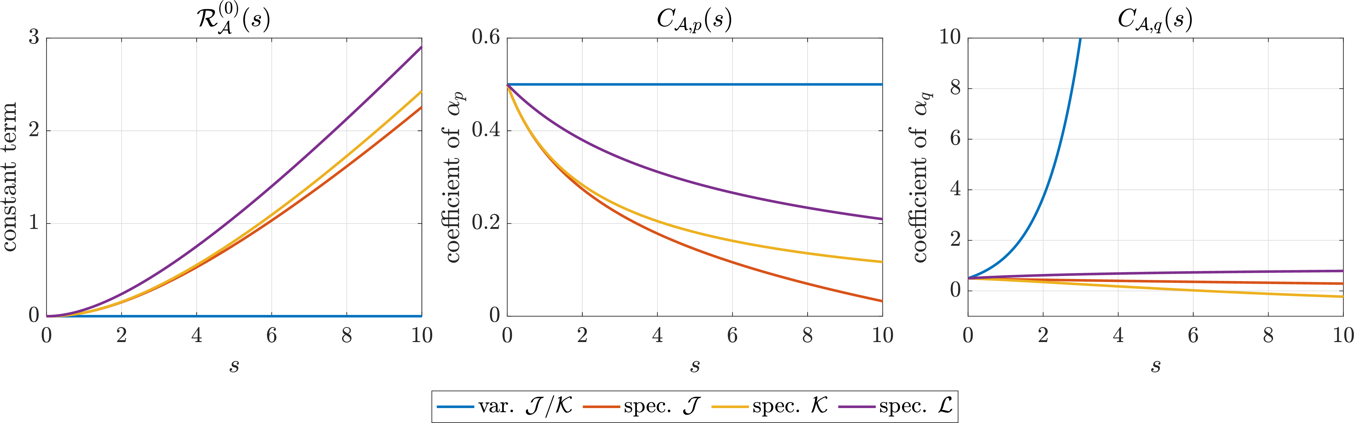
For the spectral estimator, we can expand the results of Theorem 2 for \(\alpha_p, \alpha_q\) close to zero, and derive closed form formulas for each \(\rho\), that can then be integrated over \([0,1]\). Since the formulas are overly complicated, we only plot them in Figure 1.
Figure 1 plots the three terms in Eq. (22 ). The variational estimator is correctly specified, so its population terms \(\mathcal{R}^{(0)}_{\mathcal{J},\mathrm{var}}\) and \(\mathcal{R}^{(0)}_{\mathcal{K},\mathrm{var}}\) are zero for \(\mathcal{J}\) and \(\mathcal{K}\) (while it is not for the spectral estimator). Its \(\alpha_q\)-coefficient is \(e^s/2\), which is shown in the right panel and reflects the variance of empirical exponential normalization. The spectral estimator has a nonzero population approximation term (left panel) but much weaker dependence on \(\alpha_q\) at larger fixed signal (middle and right panels).
5.2 Weak signal with proportionally small aspect ratios↩︎
We now consider the joint weak-signal/small-aspect regime \[s\downarrow0, \qquad \alpha_p=s\beta_p, \qquad \alpha_q=s\beta_q,\] where \(\beta_p,\beta_q\geqslant 0\) are fixed. Write \(\beta=\beta_p+\beta_q\). For every fixed finite pair \((\beta_p,\beta_q)\), the zero-ridge feasibility constraints are inactive for all sufficiently small \(s\): the spectral endpoint conditions \(\alpha_p<1\), \(\alpha_q<1\) hold, and the variational convex-hull radius diverges as \(\alpha_q\downarrow0\). We first start with the unregularized estimators.
Proposition 7 (Weak-signal expansion of the unregularized risks). Under \(\alpha_p=s\beta_p\), \(\alpha_q=s\beta_q\), the unregularized affine variational estimator satisfies \[\begin{align} \label{eq:weak-var-unreg-JK} \mathcal{R}_{\mathcal{J},\mathrm{var}} &=\frac{\beta}{2}s+\frac{\beta_q(1+3\beta)}{2}s^2+o(s^2),\\ \mathcal{R}_{\mathcal{K},\mathrm{var}} &=\frac{\beta}{2}s+ \Big(\frac{\beta_q(1+3\beta)}{2}+\frac{\beta_q^2}{2}\Big)s^2+o(s^2). \notag \end{align}\qquad{(8)}\] The unregularized spectral estimator satisfies \[\begin{align} \label{eq:weak-spec-unreg-JKL} \mathcal{R}_{\mathcal{J},\mathrm{spec}} &=\frac{\beta}{2}s+ \Big(\frac{1}{36}-\frac{2\beta_p}{9}-\frac{\beta_q}{18} +\frac{\beta_p^2}{12}+\frac{\beta_p\beta_q}{3}+\frac{\beta_q^2}{4}\Big) s^2+o(s^2),\\ \mathcal{R}_{\mathcal{K},\mathrm{spec}} &=\frac{\beta}{2}s+ \Big(\frac{1}{36}-\frac{2\beta_p}{9}-\frac{\beta_q}{18} +\frac{\beta_p^2}{12}+\frac{\beta_p\beta_q}{3}+\frac{3\beta_q^2}{4}\Big) s^2+o(s^2), \notag\\ \mathcal{R}_{\mathcal{L},\mathrm{spec}} &=\frac{\beta}{2}s+ \Big(\frac{1}{12}-\frac{\beta_p}{12}+\frac{\beta_q}{12} +\frac{\beta_p^2}{6}+\frac{\beta_p\beta_q}{2}+\frac{5\beta_q^2}{6}\Big) s^2+o(s^2). \notag \end{align}\qquad{(9)}\] Consequently, \[\label{eq:Qunreg-weak} \mathcal{R}_{\mathcal{J},\mathrm{spec}}-\mathcal{R}_{\mathcal{J},\mathrm{var}} =\mathcal{R}_{\mathcal{K},\mathrm{spec}}-\mathcal{R}_{\mathcal{K},\mathrm{var}} =\frac{s^2}{36}Q_{\rm unreg}(\beta_p,\beta_q)+o(s^2),\qquad{(10)}\] where \(Q_{\rm unreg}(\beta_p,\beta_q) =1-8\beta_p-20\beta_q+3\beta_p^2-42\beta_p\beta_q-45\beta_q^2.\) Thus the unregularized spectral estimator is favored to second order for criteria \(\mathcal{J}\) and \(\mathcal{K}\) when \(Q_{\rm unreg}<0\), and the affine variational estimator is favored when \(Q_{\rm unreg}>0\).
This is a Taylor expansion of the zero-ridge deterministic equivalents. For the variational estimator, the hard-limit equations of Theorem 1 yield, after tedious computations, \[\mathcal{R}_{\mathcal{J},\mathrm{var}} =\frac{\alpha_p}{2}+\frac{e^s\alpha_q}{2} +\frac{3}{2}\alpha_p\alpha_q+\frac{3}{2}\alpha_q^2+o(s^2),\] \[\mathcal{R}_{\mathcal{K},\mathrm{var}} =\frac{\alpha_p}{2}+\frac{e^s\alpha_q}{2} +\frac{3}{2}\alpha_p\alpha_q+2\alpha_q^2+o(s^2),\] valid for \(\alpha_p,\alpha_q=O(s)\). The difference is the normalizer penalty: if \(z=\log Z_q(\hat{v}_{\rm var})\), then \(z=\alpha_q+o(s)\) and \(e^z-z-1=\alpha_q^2/2+o(s^2)\). Substituting \(\alpha_p=s\beta_p\), \(\alpha_q=s\beta_q\), and \(e^s=1+s+O(s^2)\) gives Eq. (?? ).
For the spectral estimator, we can expand the zero-ridge specialization of Theorem 2 and the score formulas in Eqs. 19 21 . Integrating the resulting polynomials in \(\rho\) gives Eq. (?? ). Subtracting the variational expansion gives Eq. (?? ).
We now consider the regularized estimators, with their optimized regularization parameter.
Proposition 8 (Weak-signal expansion with optimized ridge). Let the variational ridge be parameterized by \(t=(1+\tau)^{-1}\in[0,1]\), and the spectral ridge by \(\gamma=(1+\zeta)^{-1}\in[0,1]\). For fixed \(t\), we have \[\begin{align} \mathcal{R}_{\mathcal{J},\mathrm{var}} &=\frac{s}{2}((1-t)^2+\beta t^2) +\beta_qt^3\Big(\frac{3}{2}(1+\beta)t-1\Big) s^2+o(s^2),\\ \mathcal{R}_{\mathcal{K},\mathrm{var}} &=\mathcal{R}_{\mathcal{J},\mathrm{var}}+\frac{\beta_q^2t^2}{2}s^2+o(s^2). \notag \end{align}\] The leading shrinkage problem gives \(t^\ast_{\mathcal{J},\mathrm{var}}=t^\ast_{\mathcal{K},\mathrm{var}} =\frac{1}{1+\beta}+O(s), \tau^\ast_{\mathcal{J},\mathrm{var}}=\tau^\ast_{\mathcal{K},\mathrm{var}} =\beta+O(s),\) and therefore \[\begin{align} \label{eq:weak-var-opt-ridge} \mathcal{R}^{\rm opt}_{\mathcal{J},\mathrm{var}} &=\frac{\beta}{2(1+\beta)}s+\frac{\beta_q}{2(1+\beta)^3}s^2+o(s^2),\\ \mathcal{R}^{\rm opt}_{\mathcal{K},\mathrm{var}} &=\frac{\beta}{2(1+\beta)}s+ \Big( \frac{\beta_q}{2(1+\beta)^3} +\frac{\beta_q^2}{2(1+\beta)^2}\Big) s^2+o(s^2). \notag \end{align}\qquad{(11)}\] For the spectral estimator, for each criterion \(\mathcal{A}\in\{\mathcal{J},\mathcal{K},\mathcal{L}\}\), \[\gamma^\ast_{\mathcal{A},\mathrm{spec}}=\frac{1}{1+\beta}+O(s), \qquad \zeta^\ast_{\mathcal{A},\mathrm{spec}}=\beta+O(s).\] Substituting \(\gamma=(1+\beta)^{-1}\) gives \[\begin{align} \label{eq:weak-spec-opt-ridge} \mathcal{R}^{\rm opt}_{\mathcal{J},\mathrm{spec}} &=\frac{\beta}{2(1+\beta)}s+\frac{3\beta_p+9\beta_q+1}{36(1+\beta)^3}s^2+o(s^2),\\ \mathcal{R}^{\rm opt}_{\mathcal{K},\mathrm{spec}} &=\frac{\beta}{2(1+\beta)}s+ \left\{\frac{3\beta_p+9\beta_q+1}{36(1+\beta)^3} +\frac{(2\beta_q-\beta_p)^2}{18(1+\beta)^2}\right\}s^2+o(s^2), \notag\\ \mathcal{R}^{\rm opt}_{\mathcal{L},\mathrm{spec}} &=\frac{\beta}{2(1+\beta)}s + \frac{\beta_p^3-\beta_p^2\beta_q+\beta_p^2+ \beta_p\beta_q^2-2\beta_p\beta_q+2\beta_p+ 3\beta_q^3+3\beta_q^2+4\beta_q+1}{12(1+\beta)^3}s^2+o(s^2). \notag \end{align}\qquad{(12)}\] For criterion \(\mathcal{J}\), \[\mathcal{R}^{\rm opt}_{\mathcal{J},\mathrm{spec}} -\mathcal{R}^{\rm opt}_{\mathcal{J},\mathrm{var}} =\frac{s^2}{36(1+\beta)^3}Q_{\mathcal{J},{\rm opt}}(\beta_p,\beta_q)+o(s^2),\] where \(Q_{\mathcal{J},{\rm opt}}(\beta_p,\beta_q)=1+3\beta_p-9\beta_q.\) For criterion \(\mathcal{K}\), \[\mathcal{R}^{\rm opt}_{\mathcal{K},\mathrm{spec}} -\mathcal{R}^{\rm opt}_{\mathcal{K},\mathrm{var}} =\frac{s^2}{36(1+\beta)^3}Q_{\mathcal{K},{\rm opt}}(\beta_p,\beta_q)+o(s^2),\] where \(Q_{\mathcal{K},{\rm opt}}(\beta_p,\beta_q) =1+3\beta_p-9\beta_q +2(1+\beta_p+\beta_q)(\beta_p^2-4\beta_p\beta_q-5\beta_q^2).\) Optimized spectral fitting is favored under criterion \(\mathcal{A}\in\{\mathcal{J},\mathcal{K}\}\) when the corresponding \(Q_{\mathcal{A},{\rm opt}}\) is negative.
For the variational estimator, substitute \(t=(1+\tau)^{-1}\) in the regularized fixed-signal expansion and set \(\alpha_p=s\beta_p\), \(\alpha_q=s\beta_q\). The order-\(s\) term is \(\frac{1}{2}\{(1-t)^2+\beta t^2\}s,\) whose unique minimizer is \(t=(1+\beta)^{-1}\). Since this minimizer is interior for finite \(\beta\), the order-\(s\) optimizer is enough to evaluate the risk up to order \(s^2\), giving Eq. (?? ). For the spectral estimator, expand Theorem 2 with \(\gamma=(1+\zeta)^{-1}\), \(\alpha_p=s\beta_p\), and \(\alpha_q=s\beta_q\). The leading term is the same scalar shrinkage risk with \(\gamma\) in place of \(t\), so \(\gamma^\ast=(1+\beta)^{-1}+O(s)\). Substitution into the order-\(s^2\) coefficients from the spectral score formulas gives Eq. (?? ). The formulas for \(Q_{\mathcal{J},{\rm opt}}\) and \(Q_{\mathcal{K},{\rm opt}}\) follow by subtraction.
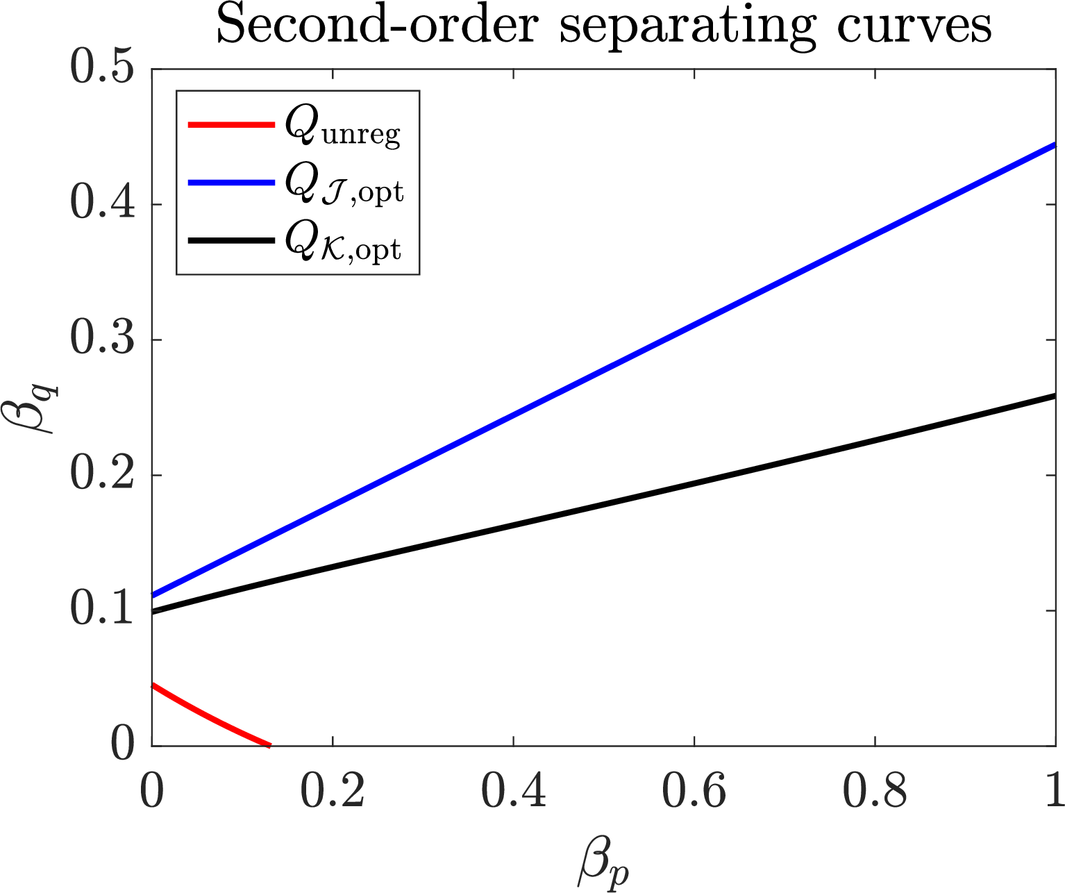
Figure 2 shows the second-order separating curves defined by \(Q_{\mathcal{K},{\rm opt}}(\beta_p,\beta_q)=0\), \(Q_{\mathcal{J},{\rm opt}}(\beta_p,\beta_q)\) and \(Q_{\rm unreg}(\beta_p,\beta_q)=0\). The unregularized curve is common to criteria \(\mathcal{J}\) and \(\mathcal{K}\), while the optimized-ridge curves differ because \(\mathcal{K}\) includes the population normalizer penalty. We see the advantage of the spectral estimator when \(\beta_q\) gets larger (fewer observations), in particular for the criterion \(\mathcal{K}\) (which characterizes the proper model normalization). While we consider here small \(s\), \(\alpha_p\), \(\alpha_q\), with explicit formulas, we consider in Section [sec:comparison] plots of the deterministic equivalents for larger values and similar conclusions.
6 Comparisons between estimators↩︎
The comparison depends on whether one asks about feasibility or population risk. The regimes below are direct consequences of Proposition 4, Proposition 5, Theorems 1 and 2, and Section [sec:zero-ridge-var].
6.0.0.1 Feasibility-first unregularized regimes.
We consider here the two unregularized (variational and spectral) estimators. Away from the boundary cases \(\alpha_q=\frac{1}{2}, \alpha_p=1, \alpha_q=1,\) the zero-ridge variational estimator is finite with high probability if and only if \[\qquad \alpha_q<\frac{1}{2} \quad\text{and}\quad s+\alpha_p<R^2_{\rm hull}(\alpha_q),\] whereas the unregularized continuum spectral full potential is finite with high probability if and only if \[\qquad \alpha_p<1 \quad\text{and}\quad \alpha_q<1 .\] This leads to the phase diagram in Figure [fig:regimes].
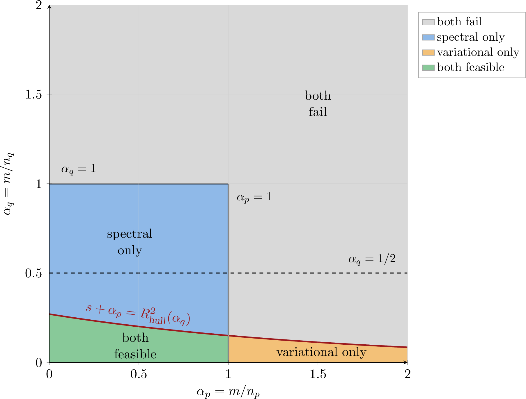

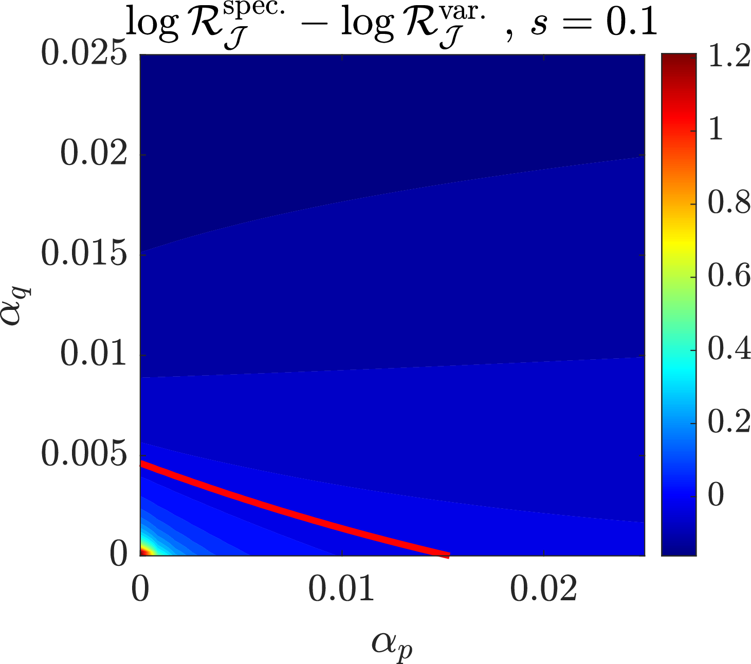
Figure 4: Comparison of two estimators for a given \(s=1\) (left) and \(s=0.1\) (right) for a fixed small regularization parameter (equal to \(10^{-8}\)). Only the difference in criterion \(\mathcal{J}\) is reported as the difference in criterion \(\mathcal{K}\) explodes. The black line (left plot) and red line (right plot) are zero-level lines..
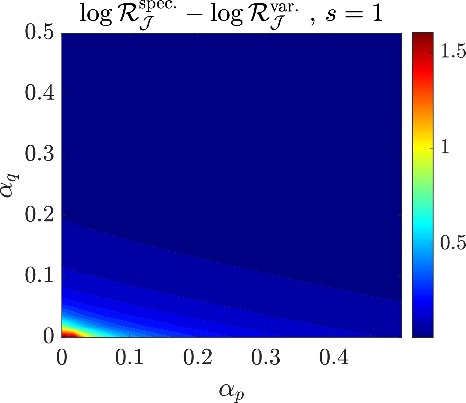
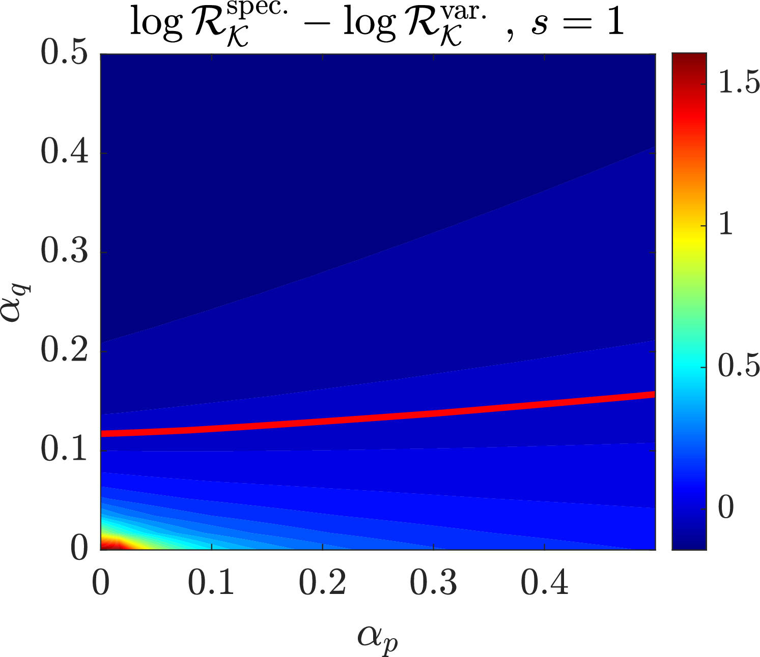
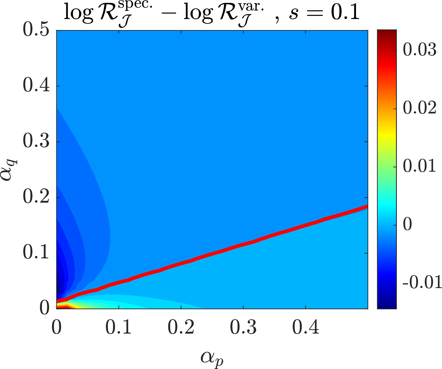
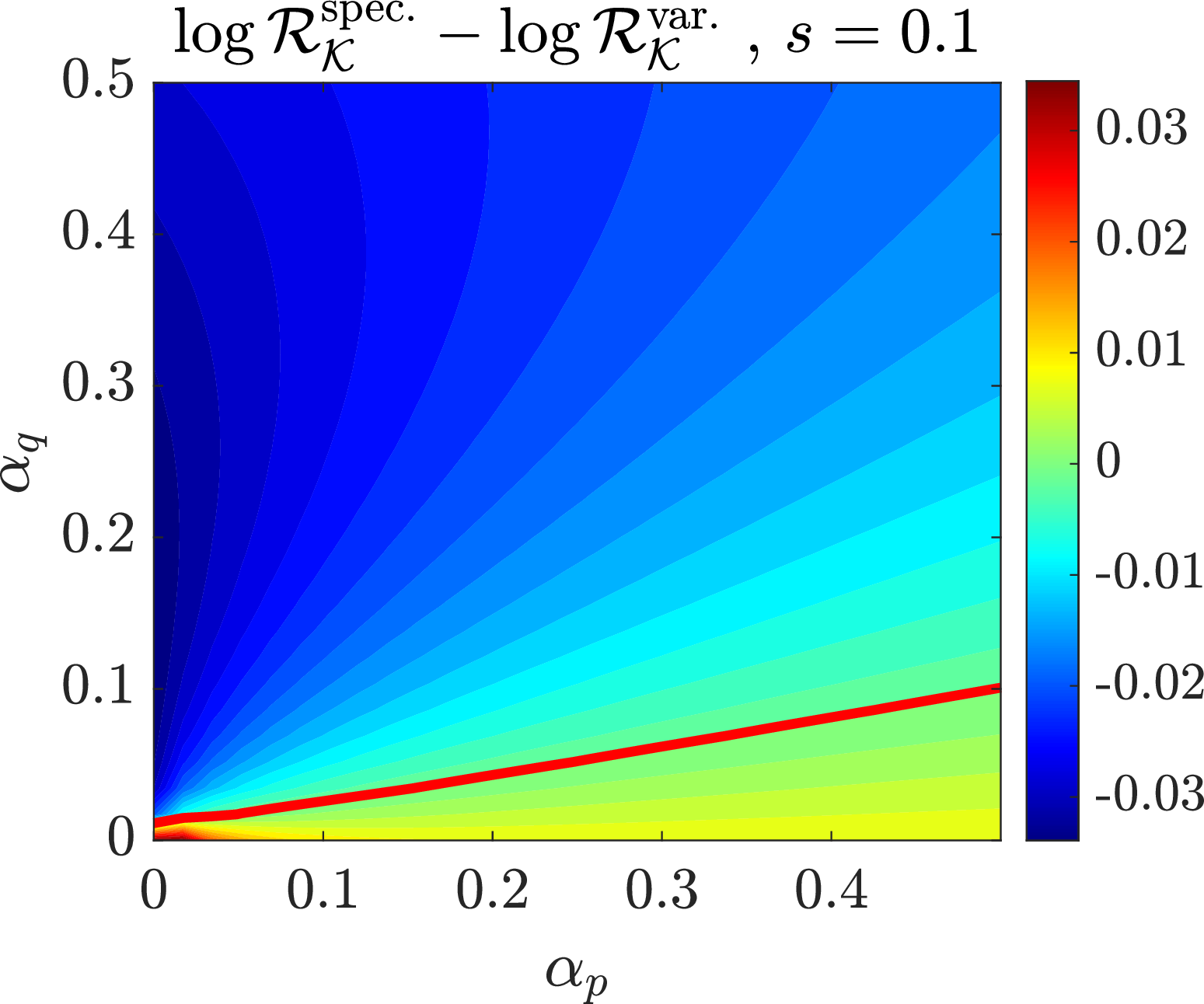
Figure 5: Comparison of two estimators for a given \(s=1\) (top) and \(s=0.1\) (bottom) when regularization parameters are optimized. Difference in criterion \(\mathcal{J}\) (left) and criterion \(\mathcal{K}\) (right). The red lines denote the zero line, above which the spectral method is better than the variational method. Note that on the top left plot (\(s=1\), criterion \(\mathcal{J}\) that is insensitive to constants), the variational method is always better..
6.0.0.2 Fixed-signal aspect-ratio unregularized regimes.
The fixed-signal contour plots in Figure 4 vary \((\alpha_p,\alpha_q)\) in \([0,1/4] \times [0,1/4]\) at a fixed value of \(s=1\) (left plot), and \((\alpha_p,\alpha_q)\) in \([0,1/40] \times [0,1/40]\) at a fixed value of \(s=0.1\) (right plot), with both regularization parameters equal to \(10^{-8}\) to mimic unregularized estimation while preserving numerical stability. In Figure 4, we show the difference \(\log(\mathcal{R}_{\mathcal{J},\rm spec}) - \log(\mathcal{R}_{\mathcal{J},\rm var})\), with the zero-level line, showing that for small \(\alpha_p, \alpha_q\), the variational method has better performance, while for larger values, the spectral estimator is better. This generalizes the plot in Figure 2 to larger values of \(s, \alpha_p,\alpha_q\).
6.0.0.3 Regularization: comparison regimes.
Figure 5 displays the criteria \[\mathcal{R}^{\rm opt}_{\mathcal{J}, \rm var} (\alpha_p,\alpha_q,s)=\inf_{\tau>0}\mathcal{R}^{\tau}_{\mathcal{J}, \rm var} (\alpha_p,\alpha_q,s), \qquad \mathcal{R}^{\rm opt}_{\mathcal{J}, \rm spec} (\alpha_p,\alpha_q,s)=\inf_{\zeta>0}\mathcal{R}^{\rm \zeta}_{\mathcal{J}, \rm spec} (\alpha_p,\alpha_q,s),\] where we now make explicit the dependence of the risks on the regularization parameter used for training. This is done under the same setup as Figure 4, but on the set \([0,1/2] \times [0,1/2]\), and for two values of \(s\) (\(s=1\) and \(s=0.1\)), and we only consider the \(\mathcal{J}\) and \(\mathcal{K}\) criteria, and plot \(\log \mathcal{R}^{\rm opt}_{\mathcal{J}, \rm spec} (\alpha_p,\alpha_q,s) - \log \mathcal{R}^{\rm opt}_{\mathcal{J}, \rm var} (\alpha_p,\alpha_q,s)\) to assess which estimator is preferable. For each value of \((\alpha_p,\alpha_q,s)\), the optimal regularization parameters are found by golden-section search plus parabolic interpolation [34]. We can draw conclusions that are similar to the ones for Figure 4.
7 Asymptotic comparisons↩︎
We consider comparisons between empirical estimation and the asymptotic results presented in Section [sec:hd], illustrating the convergence behaviors.4 We empirically illustrate a match between the asymptotic determinstic equivalents and the empirical behavior for reasonable \(m\) (as low as \(100\) for the spectral estimator, bigger for the variational one).
7.0.0.1 Varying \(m\).
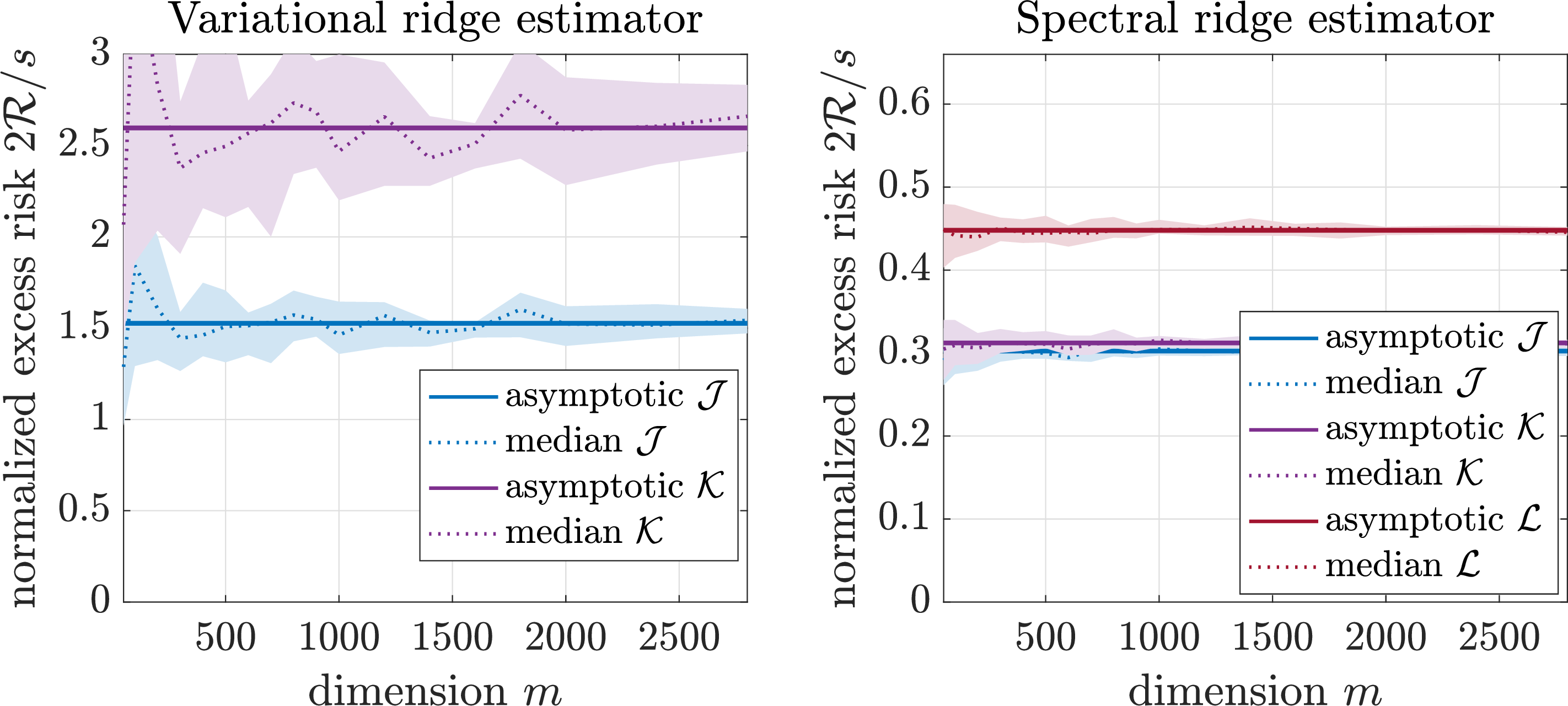
We study in Figure 6 the convergence behavior towards our asymptotic limit, with fixed \(\alpha_p=0.125\), \(\alpha_q=0.125\), and \(s=1\), with regularization parameters \(\tau = 10^{-3}\) and \(\zeta = 10^{-4}\). We vary \(m\) and plot interquartile range and median obtained from 32 replications. We see that the empirical curves converge to their asymptotic limit, with a faster convergence for the spectral estimator (right panel). We also see the differences in criteria, where \(\mathcal{K}\) measures the estimation of the normalization constants that the criterion \(\mathcal{J}\) ignores. For the spectral estimator (right panel), we see that the \(\mathcal{L}\) criterion, which uses the learned potential \(w\) (instead of replacing it with \(w=1-e^{v}\)) leads to a significantly worse result.
7.0.0.2 Varying \(\alpha_p\).
We set \(s=\|\Delta\|^2=1\) and \(m=1000\) for the variational estimator, and \(m=100\) for the spectral estimator, and for every displayed aspect ratio we draw independent samples from \(q=\mathcal{N}(0,I)\) and \(p=\mathcal{N}(\Delta,I)\). The empirical curves are averages over 16 independent replications; the shaded areas show the interquartile range across these replications. In Figure 7 and Figure 8, the ridge parameters are fixed at \(\tau=10^{-2}\) and \(\zeta=10^{-4}\). The left panel reports the ridge-regularized variational estimator under the log-normalized criterion \(\mathcal{J}\) and the Fenchel criterion \(\mathcal{K}\), whereas the right panel reports the ridge-regularized spectral estimator under \(\mathcal{J}\), \(\mathcal{K}\), and the two-potential lower-bound criterion \(\mathcal{L}\). Figure 7 fixes \(\alpha_q=0.1\) and sweeps \(\alpha_p\) uniformly over \([0,1]\) using 20 grid points; Figure 8 fixes \(\alpha_p=0.05\) and sweeps \(\alpha_q\) over the same interval. Solid curves are the proportional deterministic equivalents: the variational limits are obtained from the scalar CGMT system, while the spectral limits are evaluated by the ridge-resolvent formula using 256-point Gauss–Legendre quadrature. The empirical spectral curves are computed using the generalized-eigenvalue reduction from [1] presented in Section [sec:est2].
![Figure 7: Comparison of estimators when varying \alpha_p (\alpha_q=0.1 fixed, with \alpha_p swept over [0,1]). Left: variational, right: spectral.](/article/2607.01895/alphap_sweeps.png "fig:")
![Figure 8: Comparison of estimators when varying \alpha_q (\alpha_p=0.05 fixed, with \alpha_q swept over [0,1], only shown partially for the variational estimator since the performance is out of range). Left: variational, right: spectral.](/article/2607.01895/alphaq_sweeps.png "fig:")
8 Conclusion↩︎
8.0.0.1 Summary.
This paper compared ridge-regularized variational and spectral density-ratio estimation in a simple Gaussian location model under proportional high-dimensional asymptotics \[\frac{m}{n_p}\to\alpha_p, \qquad \frac{m}{n_q}\to\alpha_q .\] The variational estimator was analyzed through the entropy dual of the ridge-regularized log-normalized KL objective and a CGMT reduction [14]. The spectral estimator of [1] was analyzed through random-matrix deterministic equivalents for ridge resolvents of weighted sums of two independent Gaussian sample covariance matrices, in the spirit of standard resolvent methods [15], [16], but using a random feature formulation [18], [19]. These two asymptotic calculations give computable population risks for our three criteria.
At small aspect ratios (many observations), the affine variational estimator benefits from correct specification of the Gaussian log-density ratio and can have the smaller population risk. As \(\alpha_p\) and
especially \(\alpha_q\) increase, empirical exponential normalization becomes more variable: in these larger-aspect regimes (with fewer observations), the spectral estimator is preferable in the regimes identified by the
asymptotic comparison (for this simple model): it replaces empirical log-sum-exp normalization by covariance-based least-squares problems, trading some approximation bias for lower normalization variance. Positive ridge keeps both estimators finite for all
finite aspect ratios, and once optimized for regularization parameters, the spectral method is preferable for small numbers of observations (but with a reduced range of aspect values).
8.0.0.2 Extension to nuclear penalty.
In this paper, we primarily focused on an independent ridge penalty on all \(\rho\)-dependent linear predictors. In order to perform feature learning, other penalties can be considered, such as the nuclear penalty, which is classical in this context of multi-task learning [35]. Iteratively reweighted least-square formulations [36], [37] can naturally be used, both for algorithms and for the asymptotic analysis, which can now be done through matrix Dyson equations [38]. Overall, given that, for our Gaussian location model, the optimal predictors are all aligned, we see an improvement over ridge penalties. See Appendix 16 for details and derivation of deterministic equivalents a few illustrative experiments.
8.0.0.3 Extension to mutual information.
As noted in [1], a first natural extension is mutual information estimation, since it is equal to the KL divergence between a joint distribution \(p(x_1,x_2)\) and the product of its marginals. Empirically, this corresponds to comparing paired samples from the joint law with shuffled or independently paired samples from the product of marginals. This connects directly to variational mutual-information estimation and variational KL bounds [5], [6], [39], [40]. The corresponding high-dimensional question is to determine how the CGMT and random-matrix limits change when the two empirical samples come from joint and product feature distributions rather than from a Gaussian location pair. Such an analysis would give asymptotic risk predictions for variational and spectral mutual-information estimators as functions of dependence strength, feature dimension, sample size, and regularization, with in particular application to softmax regression when one of the two variables takes finitely many values.
8.0.0.4 Extension to nonlinear features.
A second extension is to replace the identity feature map by richer nonlinear features, for instance \(\varphi(x)=\sigma(Wx),\) with fixed random weights \(W\), kernel features, or features learned from data. This preserves a linear-in-parameters structure after feature construction [41], [42]. However, after the nonlinear map, the empirical design is no longer simply a Gaussian matrix or a pair of Wishart matrices. Recent high-dimensional analyses of nonlinear random-feature Gram matrices, random-feature ridge regression, Gaussian-equivalent feature models, and generic feature maps show that such problems often still admit deterministic equivalents or low-dimensional state-evolution descriptions [43]–[48]. This suggests an extension of the present CGMT and resolvent calculations in which the ambient dimension \(m\) is replaced by the effective spectral distribution of the nonlinear feature covariance or kernel matrix. The main technical question would then be to rederive the asymptotic equivalents and compare their performance.
8.0.0.5 Extension to spiked and covariance-shift models.
A third extension is to study settings where \(p\) and \(q\) differ not only in their means but also, or primarily, in their covariance matrices [15], [49], [50]. In such models, part of the signal is second-order rather than purely mean-shifted. The spectral estimator may then be structurally better aligned with the data-generating mechanism, because it is built from covariance-based least-squares problems. By contrast, an affine variational estimator would be misspecified unless augmented with quadratic or nonlinear features. These extensions would clarify whether the spectral advantage observed at larger aspect ratios is specific to the Gaussian location model, or whether it reflects a broader high-dimensional phenomenon in density-ratio and mutual-information estimation.
Tool and computational resource disclosure↩︎
During the exploratory phase of this work, the author used a large language model (GPT-pro 5.5) to explore possible applications of the convex Gaussian min-max theorem (CGMT) and random matrix theory to the problem studied in this paper, including candidate reductions, intermediate identities, and proof strategies.
All mathematical claims, statements of assumptions, and final proofs in the main paper were subsequently checked, significantly rewritten, and completed by the author. Proofs in the appendix were reviewed for correctness. The final arguments rely on the author’s own mathematical judgement and background knowledge, and no result is included solely on the basis of an LLM-generated derivation.
The same LLM was also used to assist with MATLAB code generation for numerical experiments and figure production. The resulting code was reviewed, edited, and validated by the author, including checks for consistency with the stated mathematical model and reproduction of the reported plots. All numerical experiments and figures reported in the paper were run on a single CPU.
Acknowledgements↩︎
This work has received support from the French government, managed by the National Research Agency, under the France 2030 program with the reference “PR[AI]RIE-PSAI” (ANR-23-IACL-0008).
9 Proof of Proposition 4↩︎
Write \(\mu=\hat{\mu}_p\), \(n=n_q\), and \(\Phi(\theta) = \theta^\top\mu - \log\big(\frac{1}{n}\sum_{j=1}^n \exp(\theta^\top y_j)\big).\) Let \(C=\operatorname{conv}\{y_1,\ldots,y_n\}\) and \(S=\operatorname{span}(C-C)\). If \(\mu\notin C\), strict separation gives a vector \(a\) such that \(a^\top\mu>\max_{1\leqslant j\leqslant n} a^\top y_j .\) Hence, as \(t\to\infty\), we get \(\Phi(ta) = t (a^\top\mu-\max_{j \in \{1,\dots,n\}} a^\top y_j)+O(1)\to+\infty .\) Thus the supremum is infinite.
Assume now that \(\mu\in C\). Then, for every \(\theta\), we have \(\theta^\top\mu\leqslant \max_{j \in \{1,\dots,n\}}\theta^\top y_j\) and therefore \[\Phi(\theta) \leqslant \max_{j \in \{1,\dots,n\}}\;\theta^\top y_j - \log\bigg(\frac{1}{n}\sum_{j=1}^n \exp(\theta^\top y_j)\bigg) \leqslant \log n .\] Thus the supremum is finite. Moreover, if \(h\in S^\perp\), then \(h^\top y_j\) is constant in \(j\), and since \(\mu\in C\), this constant is \(h^\top\mu\). Hence \(\Phi(\theta+h)=\Phi(\theta)\). This proves the non-identifiability modulo \(S^\perp\), and it remains to work on \(S\).
Suppose first that \(\mu\in \operatorname{ri} C\). If \(S=\{0\}\), there is nothing to prove. Otherwise, \[\delta := \inf_{\substack{u\in S\\ \|u\|=1}} \max_{j \in \{1,\dots,n\}} u^\top(y_j-\mu) >0 .\] Indeed, a zero value would give a nonzero supporting direction through \(\mu\), contradicting \(\mu\in\operatorname{ri} C\). For \(\theta=tu\in S\), with \(t=\|\theta\|\) and \(\|u\|=1\), \[\Phi(\theta) \leqslant \log n - t\max_{j \in \{1,\dots,n\}} u^\top(y_j-\mu) \leqslant \log n-\delta \|\theta\|.\] Thus \(\Phi\) is coercive from above on \(S\). Since \(\Phi\) is continuous, it attains its maximum on \(S\), and hence in \(\mathbb{R}^m\) modulo \(S^\perp\).
It remains to consider \(\mu\in C\setminus \operatorname{ri} C\). Let \(F\) be the smallest face of \(C\) containing \(\mu\), and set \(I=\{j:\;y_j\in F\}.\) Since \(C\) is a polytope, \(F\) is exposed: there exists \(a\) such that \[a^\top y_j=a^\top\mu \quad (j\in I), \qquad a^\top y_j<a^\top\mu \quad (j\notin I).\] Define the face-restricted objective \(\Phi_F(\theta) = \theta^\top\mu - \log\big(\frac{1}{n}\sum_{j\in I}\exp(\theta^\top y_j)\big).\) Since \(\mu\in\operatorname{ri}F\), the previous paragraph applied inside \(\operatorname{aff}F\) gives a maximizer \(\theta_F\) of \(\Phi_F\). Also, \(\Phi(\theta)\leqslant \Phi_F(\theta)\) for every \(\theta\). On the other hand, \(\Phi(\theta_F+ta) \longrightarrow \Phi_F(\theta_F)\) when \(t\to\infty\), because the terms with \(j\notin I\) are exponentially negligible relative to the terms with \(j\in I\). Hence \(\sup_{\theta\in\mathbb{R}^m}\Phi(\theta)=\max_{\theta}\Phi_F(\theta)<\infty .\) For every finite \(\theta\), the terms with \(j\notin I\) are strictly positive, so \(\Phi(\theta)<\Phi_F(\theta)\leqslant \max_\eta \Phi_F(\eta)=\sup_\eta \Phi(\eta).\) Thus the supremum is not attained. The sequence \(\theta_F+ta\) is a maximizing sequence escaping to infinity in a direction exposing the smallest face containing \(\mu\). Conversely, any maximizing sequence must be unbounded; otherwise a convergent subsequence would yield a finite maximizer. This completes the proof.
10 Proof of Proposition 5↩︎
Assume first that \(\hat{C}_p\succ0\) and \(\hat{C}_q\succ0\). Then, for every \(\rho\in[0,1]\), \[\hat{C}(\rho)=\rho\hat{C}_p+(1-\rho)\hat{C}_q \succcurlyeq \min\{\lambda_{\min}(\hat{C}_p),\lambda_{\min}(\hat{C}_q)\}I \succ0 .\] Hence \(\hat{M}(\rho) = \hat{C}(\rho)+\rho(1-\rho)\hat{\Delta}\hat{\Delta}^\top \succ0\) uniformly on \([0,1]\). Therefore \(\rho\mapsto \hat{M}(\rho)^{-1}\hat{\Delta}\) is continuous and bounded on \([0,1]\). Since \(\hat{\mu}(\rho)=\rho\hat{\mu}_p+(1-\rho)\hat{\mu}_q\) is also continuous, all integrands defining the coefficients in Eqs. 9 10 are continuous and bounded. Thus the unregularized full spectral potential in Eq. (11 ) is finite.
Conversely, suppose that \(\hat{C}_q\) is singular. Let \(\hat{P}_q\) denote the orthogonal projector onto \(\ker\hat{C}_q\). We first show the deterministic implication \[\hat{P}_q\hat{\Delta}\ne0 \quad\Longrightarrow\quad \text{the full potential is not finite.}\] If \(\hat{M}(\rho)\) is singular for some \(\rho\in(0,1)\), the ordinary-inverse construction is already undefined. Otherwise, set \(\hat{\beta}_\rho=\hat{M}(\rho)^{-1}\hat{\Delta} .\) From \(\hat{M}(\rho)\hat{\beta}_\rho=\hat{\Delta}\), projection onto \(\ker\hat{C}_q\) gives \(\hat{P}_q\hat{\Delta} = \rho\hat{P}_q\hat{C}_p\hat{\beta}_\rho + \rho(1-\rho)\hat{P}_q\hat{\Delta}\,\hat{\Delta}^\top\hat{\beta}_\rho ,\) because \(\hat{P}_q\hat{C}_q=0\). Hence \[\|\hat{P}_q\hat{\Delta}\| \leqslant \rho\bigl(\|\hat{C}_p\|+\|\hat{\Delta}\|^2\bigr)\|\hat{\beta}_\rho\|.\] If \(\hat{P}_q\hat{\Delta}\ne0\), then, for some constant \(c_q>0\), \(\|\hat{\beta}_\rho\|\geqslant {c_q\over \rho} ,\) with \(0<\rho<1\). Therefore \[\int_0^\varepsilon \rho(1-\rho)\|\hat{\beta}_\rho\|^2\,d\rho \geqslant c_q^2\int_0^\varepsilon {1-\rho\over \rho}\,d\rho = +\infty .\] But the quadratic coefficient satisfies \[\hat{A} = -\int_0^1 \rho(1-\rho)\hat{\beta}_\rho\hat{\beta}_\rho^\top\,d\rho ,\] so a finite full quadratic potential would imply \[\int_0^1\rho(1-\rho)\|\hat{\beta}_\rho\|^2\,d\rho<\infty .\] This contradiction proves non-finiteness at the \(q\)-endpoint.
The \(p\)-endpoint is identical. If \(\hat{C}_p\) is singular and \(\hat{P}_p\) is the orthogonal projector onto \(\ker\hat{C}_p\), then \(\hat{P}_p\hat{\Delta}\ne0\) implies, with \(\varepsilon=1-\rho\), \(\|\hat{\beta}_{1-\varepsilon}\|\geqslant {c_p\over \varepsilon}\) for some \(c_p>0\). Consequently, \[\int_{1-\varepsilon_0}^1 \rho(1-\rho)\|\hat{\beta}_\rho\|^2\,d\rho = +\infty ,\] and the full potential is again not finite.
It remains to verify that these projection conditions hold almost surely under the Gaussian sampling model. For Gaussian samples, each centered sample covariance is independent of the corresponding sample mean, and the \(p\)- and \(q\)-samples are independent. Thus \(\hat{\Delta}=\hat{\mu}_p-\hat{\mu}_q\) is independent of \(\hat{C}_p\) and \(\hat{C}_q\). Conditional on either covariance matrix, \(\hat{\Delta}\sim N\!\big(\Delta,\big({1\over n_p}+{1\over n_q}\big)I\big).\) If \(\hat{C}_q\) is singular, then \(\ker\hat{C}_q\ne\{0\}\), and conditional on \(\hat{C}_q\), \(\hat{P}_q\hat{\Delta}\) is a nondegenerate Gaussian vector on \(\ker\hat{C}_q\), with covariance \(\big({1\over n_p}+{1\over n_q}\big)\hat{P}_q .\) Therefore \(\mathbb{P}(\hat{P}_q\hat{\Delta}=0\mid \hat{C}_q)=0\) on the event that \(\hat{C}_q\) is singular. The same argument gives \(\mathbb{P}(\hat{P}_p\hat{\Delta}=0\mid \hat{C}_p)=0\) on the event that \(\hat{C}_p\) is singular.
Finally, centered Gaussian sample covariances have ranks \(\operatorname{rank}(\hat{C}_p)=\min(m,n_p-1),\) \(\operatorname{rank}(\hat{C}_q)=\min(m,n_q-1)\) almost surely. Hence \(\hat{C}_p\succ0 \Leftrightarrow n_p\geqslant m+1, \hat{C}_q\succ0 \Leftrightarrow n_q\geqslant m+1\) almost surely. Combining the positive-definite case with the endpoint-divergence argument proves that the unregularized continuum spectral full potential is finite almost surely if and only if \(n_p,n_q\geqslant m+1 .\)
11 Detailed computations for Section [sec:specpop]↩︎
Set \[a=1+\zeta,\qquad g(\rho)=\rho(1-\rho),\qquad D(\rho)=a+s g(\rho),\qquad t=\Delta^\top x .\] At the population level, we have \[M_0(\rho)+\zeta I = (1+\zeta)I+\rho(1-\rho)\Delta\Delta^\top = aI+g(\rho)\Delta\Delta^\top .\] Since \(\|\Delta\|^2=s\), \[\{aI+g(\rho)\Delta\Delta^\top\}\Delta = (a+s g(\rho))\Delta = D(\rho)\Delta .\] Therefore \[\beta^{(0)}(\rho)=\frac{\Delta}{D(\rho)}, \qquad u^{(0)}(\rho)(x) = \beta^{(0)}(\rho)^\top(x-\rho\Delta) = \frac{t-\rho s}{D(\rho)}.\]
We use throughout \[h(s)=\int_0^1\frac{d\rho}{D(\rho)} = \int_0^1\frac{d\rho}{a+s\rho(1-\rho)} ,\] where the derivative \(h'(s)\) is taken with respect to \(s\), keeping \(a=1+\zeta\) fixed. Thus \[h'(s) = -\int_0^1\frac{g(\rho)}{D(\rho)^2}\,d\rho .\] For \(s>0\), the closed form is obtained by writing \(\rho=1/2+z\): \[h(s) = \int_{-1/2}^{1/2} \frac{dz}{a+s/4-sz^2} = \frac{4}{\sqrt{s\{s+4a\}}} \operatorname{arctanh} \sqrt{\frac{s}{s+4a}},\] with continuous extension \(h(0)=\frac{1}{a}.\)
We first record the elementary integral identities used below. By symmetry of \(D(\rho)\) under \(\rho\mapsto 1-\rho\), \[\int_0^1\frac{\rho}{D(\rho)}\,d\rho = \int_0^1\frac{1-\rho}{D(\rho)}\,d\rho = \frac{h(s)}{2}, \quadand\quad \int_0^1\frac{\rho g(\rho)}{D(\rho)^2}\,d\rho = \int_0^1\frac{(1-\rho)g(\rho)}{D(\rho)^2}\,d\rho = -\frac{h'(s)}{2}.\] Moreover, since \(D(\rho)=a+s g(\rho)\), \[\int_0^1\frac{g(\rho)}{D(\rho)}\,d\rho = \frac{1-a h(s)}{s}, \quadand\quad \int_0^1\frac{g(\rho)^2}{D(\rho)^2}\,d\rho = \frac{1-a h(s)}{s^2} + \frac{a}{s}h'(s).\] Also, \[\int_0^1\frac{d\rho}{D(\rho)^2} = \frac{h(s)+s h'(s)}{a},\] because \[h(s) = \int_0^1\frac{D(\rho)}{D(\rho)^2}\,d\rho = a\int_0^1\frac{d\rho}{D(\rho)^2} + s\int_0^1\frac{g(\rho)}{D(\rho)^2}\,d\rho .\] Consequently, \[\int_0^1\frac{(1-\rho)^2}{D(\rho)^2}\,d\rho = \frac{1}{2}\int_0^1\frac{d\rho}{D(\rho)^2} - \int_0^1\frac{g(\rho)}{D(\rho)^2}\,d\rho = \frac{h(s)+(s+2a) h'(s)}{2a}.\] The identities containing \(1/s\) are intermediate identities for \(s>0\); the final formulas below extend continuously to \(s=0\).
We now compute \(v_{\mathrm{spec}}^{(0)}\). By definition, \[v_{\mathrm{spec}}^{(0)}(x) = \int_0^1 2(1-\rho) \left( u_0(\rho)(x)-\frac{\rho}{2}u_0(\rho)(x)^2 \right)\,d\rho .\] Substituting \(u^{(0)}(\rho)(x)=(t-\rho s)/D(\rho)\) gives \[v_{\mathrm{spec}}^{(0)}(x) = \int_0^1 \left[ \frac{2(1-\rho)(t-\rho s)}{D(\rho)} - \frac{\rho(1-\rho)(t-\rho s)^2}{D(\rho)^2} \right]\,d\rho .\] Hence \(v_{\mathrm{spec}}^{(0)}\) is a scalar quadratic polynomial in \(t=\Delta^\top x\): \[v_{\mathrm{spec}}^{(0)}(x) = A_v(s)t^2+B_v(s)t+C_v(s).\] The quadratic coefficient is \[A_v(s) = -\int_0^1\frac{g(\rho)}{D(\rho)^2}\,d\rho = h'(s).\] The linear coefficient is \[\begin{align} B_v(s) &= 2\int_0^1\frac{1-\rho}{D(\rho)}\,d\rho + 2s\int_0^1\frac{\rho g(\rho)}{D(\rho)^2}\,d\rho = h(s)-s h'(s). \end{align}\] For the constant coefficient, \[\begin{align} C_v(s) &= -2s\int_0^1\frac{g(\rho)}{D(\rho)}\,d\rho - s^2\int_0^1\frac{\rho^2 g(\rho)}{D(\rho)^2}\,d\rho . \end{align}\] Since \(\rho^2=\rho-g(\rho)\), \[\int_0^1\frac{\rho^2 g(\rho)}{D(\rho)^2}\,d\rho = \int_0^1\frac{\rho g(\rho)}{D(\rho)^2}\,d\rho - \int_0^1\frac{g(\rho)^2}{D(\rho)^2}\,d\rho = -\frac{h'(s)}{2} - \left( \frac{1-a h(s)}{s^2} + \frac{a}{s}h'(s) \right).\] Therefore \[\begin{align} C_v(s) &= -2\{1-a h(s)\} + \frac{s^2}{2}h'(s) + \{1-a h(s)\} + a s h'(s) = a h(s)-1+\left(a s+\frac{s^2}{2}\right)h'(s). \end{align}\] Thus \[v_{\mathrm{spec}}^{(0)}(x) = h'(s)t^2 + \{h(s)-s h'(s)\}t + a h(s)-1 + \left(a s+\frac{s^2}{2}\right)h'(s), \qquad t=\Delta^\top x,\quad a=1+\zeta .\]
We next compute the companion potential \(w_{\mathrm{spec}}^{(0)}\). By definition, \[w_{\mathrm{spec}}^{(0)}(x) = \int_0^1 2(1-\rho) \left( -u_0(\rho)(x)-\frac{1-\rho}{2}u_0(\rho)(x)^2 \right)\,d\rho .\] Substituting \(u^{(0)}(\rho)(x)=(t-\rho s)/D(\rho)\) gives \[w_{\mathrm{spec}}^{(0)}(x) = \int_0^1 \left[ -\frac{2(1-\rho)(t-\rho s)}{D(\rho)} - \frac{(1-\rho)^2(t-\rho s)^2}{D(\rho)^2} \right]\,d\rho .\] Thus \[w_{\mathrm{spec}}^{(0)}(x) = A_w(s)t^2+B_w(s)t+C_w(s).\] The quadratic coefficient is \[A_w(s) = -\int_0^1\frac{(1-\rho)^2}{D(\rho)^2}\,d\rho = -\frac{h(s)+(s+2a)h'(s)}{2a}.\] The linear coefficient is \[\begin{align} B_w(s) &= -2\int_0^1\frac{1-\rho}{D(\rho)}\,d\rho + 2s\int_0^1\frac{\rho(1-\rho)^2}{D(\rho)^2}\,d\rho = -h(s)-s h'(s), \end{align}\] because \[\int_0^1\frac{\rho(1-\rho)^2}{D(\rho)^2}\,d\rho = \int_0^1\frac{(1-\rho)g(\rho)}{D(\rho)^2}\,d\rho = -\frac{h'(s)}{2}.\] Finally, \[\begin{align} C_w(s) &= 2s\int_0^1\frac{g(\rho)}{D(\rho)}\,d\rho - s^2\int_0^1\frac{g(\rho)^2}{D(\rho)^2}\,d\rho \\ &= 2(1-a h(s)) - \left( 1-a h(s)+a s h'(s) \right) = 1-a h(s)-a s h'(s). \end{align}\] Therefore \[w_{\mathrm{spec}}^{(0)}(x) = -\frac{h(s)+(s+2a)h'(s)}{2a}t^2 - (h(s)+s h'(s))t + 1-a h(s)-a s h'(s), \qquad t=\Delta^\top x,\quad a=1+\zeta .\]
12 Proof of Theorem 1↩︎
We write \[n=n_q,\qquad \frac{m}{n}\to \alpha=\alpha_q, \qquad r^2=s+\alpha_p,\] and denote the \(q\)-sample matrix by \(Y = (y_1,\dots,y_n)^\top \in\mathbb{R}^{n\times m}.\) Thus \(Y u\in\mathbb{R}^n\) has entries \(y_j^\top u\), and \(Y^\top a=\sum_{j=1}^n a_jy_j\). We first condition on \(\hat{\mu}_p=\mu\). It is enough to prove the conditional result for any sequence of deterministic vectors \(\mu=\mu_n\) such that \[\|\mu\|^2\to r^2, \qquad \Delta^\top\mu\to s.\] Indeed, \(\hat{\mu}_p\) is independent of the \(q\)-sample, and these two limits hold in probability under Assumption 1; the unconditional result follows by conditioning. We prove the nondegenerate case \(s+\alpha_p+\alpha_q>0\), which is the case in which the displayed formulas with \(B^{-1}\) are used. If \(s=\alpha_p=\alpha_q=0\), the limiting entropy problem has the unique optimizer \(A\equiv1\), the limiting coefficient is \(\xi=0\), and the fitted affine potential converges to zero, giving \(J_{\rm var}=K_{\rm var}=0\).
Let \[h(a)=a\log a-a+1, \qquad a\geqslant 0,\] with the convention \(h(0)=1\).
Step 1: ridge entropy dual. For every \(z\in\mathbb{R}^n\), the entropy conjugacy of log-sum-exp gives \[\log\bigg(\frac{1}{n}\sum_{j=1}^n e^{z_j}\bigg) = \sup_{\substack{a\in\mathbb{R}_+^n\\ n^{-1}\sum_{j=1}^n a_j=1}} \frac{1}{n} a^\top z-\frac{1}{n}\sum_{j=1}^n a_j\log a_j .\] Since \(n^{-1}\sum_j a_j=1\), the entropy term may equivalently be written as \(n^{-1}\sum_j h(a_j)\). Applying this identity to \(z=Y\theta\), and using strong concavity in the ridge coefficient, gives \[\begin{align} &\max_{\theta\in\mathbb{R}^m} \theta^\top\mu -\log\bigg(\frac{1}{n}\sum_{j=1}^n e^{y_j^\top\theta}\bigg) -\frac{\tau}{2}\|\theta\|^2 \\ &\quad = \min_{\substack{a\in\mathbb{R}_+^n\\ n^{-1}\sum_{j=1}^n a_j=1}} \max_{u\in\mathbb{R}^m} \frac{1}{n}\sum_{j=1}^n h(a_j) +u^\top\mu -\frac{1}{n} u^\top Y^\top a -\frac{\tau}{2}\|u\|^2 \\ &\quad = \min_{\substack{a\in\mathbb{R}_+^n\\ n^{-1}\sum_{j=1}^n a_j=1}} \frac{1}{n}\sum_{j=1}^n h(a_j) +\frac{1}{2\tau}\left\|\mu-\frac{1}{n}Y^\top a\right\|^2 . \end{align}\] The maximizer over \(u\) is \(u=\frac{1}{\tau}\left(\mu-\frac{1}{n}Y^\top a\right).\) At the saddle point this vector is the fitted ridge coefficient, hence \(\hat{\theta} =\frac{1}{\tau}\left(\mu-\frac{1}{n}Y^\top a\right).\) Thus the ridge penalty replaces the zero-ridge moment constraint \(n^{-1}Y^\top a=\mu\) by a squared residual penalty.
Step 2: compact CGMT reduction. For fixed \(a\), dualize the squared norm as \[\frac{1}{2\tau}\left\|\mu-\frac{1}{n}Y^\top a\right\|^2 = \sup_{u\in\mathbb{R}^m} u^\top\mu-\frac{1}{n} u^\top Y^\top a-\frac{\tau}{2}\|u\|^2 .\] Fix \(0<\varepsilon<1<M\) and \(R<\infty\), and consider the compact primary optimization \[\begin{align} \varphi_{n,\tau}^{\varepsilon,M,R}(\mu) = \min_{\substack{a\in[\varepsilon,M]^n\\ n^{-1}\sum_{j=1}^n a_j=1}} \max_{\|u\|\leqslant R} \frac{1}{n}\sum_{j=1}^n h(a_j) +u^\top\mu -\frac{1}{n} u^\top Y^\top a -\frac{\tau}{2}\|u\|^2. \end{align}\] This is convex in \(a\) and concave in \(u\) on compact convex sets. The CGMT auxiliary optimization has independent standard Gaussian vectors \(g\in\mathbb{R}^m\) and \(h \in\mathbb{R}^n\), and replaces the bilinear Gaussian term by \[-\frac{1}{n} u^\top Y^\top a \quad\leadsto\quad \frac{\|a\|}{n}g^\top u-\frac{\|u\|}{n}h^\top a.\] Hence \[\begin{align} \widetilde{\varphi}_{n,\tau}^{\varepsilon,M,R}(\mu) = \min_{\substack{a\in[\varepsilon,M]^n\\ n^{-1}\sum_{j=1}^n a_j=1}} \max_{\|u\|\leqslant R} \frac{1}{n}\sum_{j=1}^n h(a_j) +u^\top\mu +\frac{\|a\|}{n}g^\top u -\frac{\|u\|}{n}h^\top a -\frac{\tau}{2}\|u\|^2 . \end{align}\] For fixed \(a\), define \[Z_a=\mu+\frac{\|a\|}{n}g, \qquad \ell_a=\frac{1}{n}h^\top a.\] Optimizing over the direction of \(u\), and writing \(\xi=\|u\|\), gives \[\begin{align} \widetilde{\varphi}_{n,\tau}^{\varepsilon,M,R}(\mu) = \min_{\substack{a\in[\varepsilon,M]^n\\ n^{-1}\sum_{j=1}^n a_j=1}} \max_{0\leqslant \xi\leqslant R} \frac{1}{n}\sum_{j=1}^n h(a_j) +\xi\{\|Z_a\|-\ell_a\} -\frac{\tau}{2}\xi^2 . \end{align}\] If the radius constraint \(\xi\leqslant R\) is removed, the maximization over \(\xi\geqslant0\) equals \(\frac{1}{2\tau}(\|Z_a\|-\ell_a)_+^2,\) which is the source of the positive-part square in Eq. (?? ).
Step 3: deterministic limit of the auxiliary problem. Uniformly over \(a\in[\varepsilon,M]^n\), \[\begin{align} \|Z_a\|^2 &= \left\|\mu+\frac{\|a\|}{n}g\right\|^2 = \|\mu\|^2 +2\frac{\|a\|}{n}\mu^\top g +\frac{\|a\|^2}{n^2}\|g\|^2. \end{align}\] Conditionally on \(\mu\), \(\mu^\top g=O_{\mathbb{P}}(1)\), while \(\|a\|/n\leqslant M n^{-1/2}\). Hence the cross term is \(o_{\mathbb{P}}(1)\), uniformly over the compact set. Also, \[\frac{\|a\|^2}{n^2}\|g\|^2 = \bigg(\frac{1}{n}\sum_{j=1}^n a_j^2\bigg) \bigg(\frac{m}{n}\frac{\|g\|^2}{m}\bigg) = \alpha_q\bigg(\frac{1}{n}\sum_{j=1}^n a_j^2\bigg)+o_{\mathbb{P}}(1),\] uniformly over \(a\in[\varepsilon,M]^n\). Thus the vector \(g\) self-averages into the scalar radius \[B_n(a)= \bigg( \|\mu\|^2+ \alpha_q\frac{1}{n}\sum_{j=1}^n a_j^2 \bigg)^{1/2}.\] The vector \(h\) remains in the coordinatewise average \(n^{-1}\sum_j a_jH_j\). Passing to empirical occupation measures \(n^{-1}\sum_j\delta_{(H_j,a_j)}\), every subsequential limit has first marginal \(\mathcal{N}(0,1)\). Conditional randomization of the second coordinate given \(H\) cannot improve the infimum: replacing the second coordinate by its conditional mean preserves \(\mathbb{E}[A]\) and \(\mathbb{E}[AH]\), and Jensen’s inequality decreases both \(\mathbb{E}[h(A)]\) and \(\mathbb{E}[A^2]\). Therefore it is enough in the limit to optimize over deterministic measurable selectors \(A=A(H)\), where \(H\sim\mathcal{N}(0,1)\).
For such a selector define \[B(A)=\left(r^2+\alpha\mathbb{E}[A^2]\right)^{1/2}.\] The compact deterministic auxiliary limit is \[\begin{align} \psi_{\varepsilon,M,R}(r) = \inf_{\substack{A(H)\in[\varepsilon,M]\\ \mathbb{E}[A]=1}} \sup_{0\leqslant \xi\leqslant R} \mathbb{E}[h(A)] +\xi\{B(A)-\mathbb{E}[AH]\} -\frac{\tau}{2}\xi^2. \end{align}\] The preceding uniform approximation and the standard sample-average / epi-convergence argument give \[\widetilde{\varphi}_{n,\tau}^{\varepsilon,M,R}(\mu) \xrightarrow{\mathbb{P}} \psi_{\varepsilon,M,R}(r).\] The compact CGMT [30] transfers the same limit to the primary problem \(\varphi_{n,\tau}^{\varepsilon,M,R}(\mu) \xrightarrow{\mathbb{P}} \psi_{\varepsilon,M,R}(r).\)
It remains to remove the compact restrictions. The feasible point \(a_j\equiv1\) gives an \(O_{\mathbb{P}}(1)\) upper bound on the untruncated objective. Hence every near minimizer has bounded empirical entropy and bounded residual \(\|\mu-n^{-1}Y^\top a\|\). The entropy bound gives uniform integrability of the weights, and the residual bound gives tightness of the associated dual vector \(u=\tau^{-1}(\mu-n^{-1}Y^\top a)\). Truncating the weights to \([\varepsilon,M]\), renormalizing them to have empirical mean one, and then letting \(\varepsilon\downarrow0\), \(M\to\infty\) gives the same epigraphical limit; finally let \(R\to\infty\). Denote the corresponding untruncated value by \[\begin{align} \varphi_{n,\tau}(\mu) = \min_{\substack{a\in\mathbb{R}_+^n\\ n^{-1}\sum_{j=1}^n a_j=1}} \frac{1}{n}\sum_{j=1}^n h(a_j) +\frac{1}{2\tau}\left\|\mu-\frac{1}{n}Y^\top a\right\|^2 . \end{align}\] Consequently, \(\varphi_{n,\tau}(\mu)\) converges in probability to \[\begin{align} \psi_\tau(r) &= \inf_{\substack{A\geqslant0\\ \mathbb{E}[A]=1}} \mathbb{E}[h(A)] +\frac{1}{2\tau}(B(A)-\mathbb{E}[AH])_+^2 \\ &= \inf_{\substack{A\geqslant0\\ \mathbb{E}[A]=1}} \mathbb{E}[A\log A-A+1] +\frac{1}{2\tau} \left( \left(r^2+\alpha\mathbb{E}[A^2]\right)^{1/2}-\mathbb{E}[AH] \right)_+^2 , \end{align}\] which is Eq. (?? ) after substituting \(r^2=s+\alpha_p\) and \(\alpha=\alpha_q\).
Step 4: uniqueness and KKT equations. The feasible set \(\{A\geqslant0:\mathbb{E}[A]=1\}\) is convex. The entropy term \(\mathbb{E}[h(A)]\) is strictly convex, while \[A\longmapsto \left( \left(r^2+\alpha\mathbb{E}[A^2]\right)^{1/2}-\mathbb{E}[AH] \right)_+^2\] is convex: \(A\mapsto (r^2+\alpha\mathbb{E}[A^2])^{1/2}\) is a norm-type convex functional, subtracting the linear term \(\mathbb{E}[AH]\) preserves convexity, positive-part preserves convexity, and squaring preserves convexity on \([0,\infty)\). Entropy sublevel sets are uniformly integrable, and the remaining terms are lower semicontinuous under the induced weak convergence. Thus the limiting problem has a unique optimizer, denoted \(A\). Moreover \(A>0\) almost surely: if \(A=0\) on a set of positive Gaussian measure, then increasing \(A\) slightly on a bounded subset of that set and compensating the mass elsewhere gives a first-order entropy decrease with slope \(-\infty\), whereas the penalty term has finite one-sided variation.
Since \(s+\alpha_p+\alpha_q>0\), the optimizer is nondegenerate and \(B=B(A)>0\). The positive-part term is strictly active. Otherwise the penalty has zero derivative, and the stationarity of the entropy under the mass constraint would force \(A\) to be constant; the constraint \(\mathbb{E}[A]=1\) then gives \(A\equiv1\), for which \(B(A)-\mathbb{E}[AH]=(r^2+\alpha)^{1/2}>0\), a contradiction. Therefore \[\xi=\frac{B-\mathbb{E}[AH]}{\tau}>0, \qquad \mathbb{E}[AH]=B-\tau\xi.\] For variations \(\delta A\) preserving integrability, \(\delta B(A)=\frac{\alpha}{B}\mathbb{E}[A\,\delta A]\). Introducing a multiplier \(\lambda\) for the constraint \(\mathbb{E}[A]=1\), the first variation of \(\mathbb{E}[h(A)]+\frac{1}{2\tau}(B(A)-\mathbb{E}[AH])^2+\lambda(\mathbb{E}[A]-1)\) is \(\mathbb{E}[(\log A+\xi(\frac{\alpha}{B}A-H)+\lambda)\delta A]\). Absorbing \(-\lambda\) into \(\eta\), stationarity gives \[\log A+\frac{\xi\alpha}{B}A= \eta+\xi H \qquad\text{almost surely}.\] Together with the mass constraint, the definition of \(B\), and the active relation above, this yields \[\mathbb{E}[A]=1, \qquad r^2+\alpha\mathbb{E}[A^2]=B^2, \qquad \mathbb{E}[AH]=B-\tau\xi.\] After substituting \(r^2=s+\alpha_p\) and \(\alpha=\alpha_q\), these are Eqs. ?? ?? . For fixed \((\xi,B,\eta)\), the map \(a\mapsto \log a+(\xi\alpha/B)a\) is strictly increasing on \((0,\infty)\), so the scalar KKT equation determines \(A(H)\) uniquely.
Step 5: optimizer observables. To identify projections of the primary optimizer, we use the optimizer-localization consequence of the CGMT [51] through a perturbation argument. Fix a deterministic sequence \(v\in\mathbb{R}^m\) with bounded norm and add the linear perturbation \(\lambda v^\top u\) to the compact primary problem, equivalently replacing \(\mu\) by \(\mu+\lambda v\). The compact CGMT and the same truncation-removal argument apply locally uniformly for \(\lambda\) in a neighborhood of zero. Hence the perturbed primary values converge locally uniformly, in probability, to the corresponding deterministic perturbed value. Since the finite-\(n\) value is differentiable at \(\lambda=0\), with derivative \(\hat{\theta}^\top v\), and since the limiting variational problem has a unique optimizer, Danskin’s envelope theorem gives the derivative of the limiting value. The standard convergence theorem for derivatives of locally uniformly convergent convex functions then yields convergence of the optimizer observable.
The limiting derivative is obtained by differentiating \[B_\lambda(A)= \left(\|\mu+\lambda v\|^2+ \alpha\mathbb{E}[A^2]\right)^{1/2}\] at the optimizer, hence equals \(\xi\frac{\mu^\top v}{B}\). Taking \(v=\mu\) and \(v=\Delta\), and using \(\|\mu\|^2\to r^2\) and \(\Delta^\top\mu\to s\), gives \[\hat{\theta}^\top\mu\to \frac{\xi r^2}{B}, \qquad \hat{\theta}^\top\Delta\to \frac{\xi s}{B}.\] Similarly, differentiating the finite-\(n\) value with respect to \(\tau\) gives \(-\|\hat{\theta}\|^2/2\), while differentiating the deterministic limit with respect to \(\tau\) gives \(-\xi^2/2\). Hence \(\|\hat{\theta}\|^2\to\xi^2,\hat{\theta}^\top\Delta\to\frac{\xi s}{B}\), which proves ?? .
The entropy of the fitted dual weights is also determined by the value convergence. For the optimizer \(a\), \[\varphi_{n,\tau}(\mu) = \frac{1}{n}\sum_{j=1}^n h(a_j) +\frac{\tau}{2}\|\hat{\theta}\|^2,\] because \(\mu-n^{-1}Y^\top a=\tau\hat{\theta}\). The deterministic value is \[\psi_\tau(r)=\mathbb{E}[h(A)]+\frac{\tau}{2}\xi^2,\] since \(B-\mathbb{E}[AH]=\tau\xi\). Therefore \(\frac{1}{n}\sum_{j=1}^n h(a_j) \to \mathbb{E}[h(A)].\) The finite-\(n\) and limiting mass constraints give \(\frac{1}{n}\sum_{j=1}^n a_j\log a_j \to \mathbb{E}[A\log A].\)
It remains to identify the empirically normalized intercept. At the saddle point, the entropy-dual weights are the empirical exponential weights, \[a_j= \exp\{y_j^\top\hat{\theta}+\hat{c}\}, \qquad \hat{c}=-\log\bigg(\frac{1}{n}\sum_{j=1}^n e^{y_j^\top\hat{\theta}}\bigg),\] and \(n^{-1}\sum_ja_j=1\). Therefore \[\begin{align} \frac{1}{n}\sum_{j=1}^n a_j\log a_j &= \hat{\theta}^\top\Big(\frac{1}{n}Y^\top a\Big) +\hat{c}\bigg(\frac{1}{n}\sum_{j=1}^na_j\bigg) = \hat{\theta}^\top(\mu-\tau\hat{\theta})+\hat{c}. \end{align}\] Thus \(\hat{c}= \frac{1}{n}\sum_{j=1}^n a_j\log a_j -\hat{\theta}^\top\mu +\tau\|\hat{\theta}\|^2.\) Using the limits just proved, \[\hat{c} \to \mathbb{E}[A\log A]+\tau\xi^2-\frac{\xi r^2}{B} = \mathbb{E}[A\log A]+\tau\xi^2-\frac{\xi(s+\alpha_p)}{B},\] which proves Eq. (?? ).
For the fitted affine potential \(\hat{v}_{\rm var}(x)=\hat{\theta}^\top x+\hat{c}\), the population \(q\)-log-normalizer satisfies \[\log Z_q(\hat{v}_{\rm var}) =\hat{c}+\frac{1}{2}\|\hat{\theta}\|^2 \to z:= \mathbb{E}[A\log A]+\tau\xi^2-\frac{\xi(s+\alpha_p)}{B} +\frac{1}{2}\xi^2.\] By Proposition 1, \[J(\hat{v}_{\rm var}) =\hat{\theta}^\top\Delta-\frac{1}{2}\|\hat{\theta}\|^2 \to J_{\rm var}:=\frac{\xi s}{B}-\frac{1}{2}\xi^2.\] Using the identity \(K(v)=J(v)+\log Z_q(v)-Z_q(v)+1\), we also get \(K(\hat{v}_{\rm var}) \to K_{\rm var}:=J_{\rm var}+z-e^z+1.\) Equivalently, the excess risks satisfy \(\mathcal{R}^{\rm var}_{\mathcal{J}} \to \frac{s}{2}-J_{\rm var} = \frac{1}{2}\left(s+\xi^2-2\frac{\xi s}{B}\right),\) and \(\mathcal{R}^{\rm var}_{\mathcal{K}} \to \mathcal{R}^{\rm var}_{\mathcal{J}}+e^z-z-1.\) This proves the stated score limits, and separately records the corresponding risk limits.
13 Feasibility of the zero-ridge variational limit (Section [sec:zero-ridge-var])↩︎
Let \(H \sim \mathcal{N}(0,1)\). Define \[\varphi(z)=\frac{1}{\sqrt{2\pi}}e^{-z^2/2}, \qquad \bar\Phi(z)=\mathbb{P}(H\geqslant z)=1-\Phi(z).\] For \(\alpha\geqslant 0\), set \[\label{eq:appE-rhull-def} R_{\rm hull}^2(\alpha) = \sup_{A\geqslant 0,\;\mathbb{E}[A]=1} \bigl(\mathbb{E}[AH]\bigr)^2-\alpha \mathbb{E}[A^2] .\tag{23}\]
We compute this quantity explicitly. First, if \(\alpha=0\), then \(R_{\rm hull}^2(0)=+\infty.\) Indeed, with \(A_t(H)=\frac{ 1_{\{H\geqslant t\}}}{\bar\Phi(t)},\) we have \(\mathbb{E}[A_t]=1\) and \(\mathbb{E}[A_tH]= {\varphi(t)}/{\bar\Phi(t)}\sim t\) tends to infinity when \(t\to+\infty,\) so the objective in Eq. (23 ) is unbounded.
Assume now that \(\alpha>0\). Using \(x^2=\sup_{u\in\mathbb{R}}\{2ux-u^2\},\) we may write \[\label{eq:appE-rhull-dual} R_{\rm hull}^2(\alpha) = \sup_{u\in\mathbb{R}} \Big\{ -u^2+ \sup_{A\geqslant0,\;\mathbb{E}[A]=1} \mathbb{E}\bigl[2uHA-\alpha A^2\bigr] \Big\}.\tag{24}\] By symmetry of \(H\), it is enough to consider \(u\geqslant 0\). For fixed \(u>0\), the inner problem is concave in \(A\). Its KKT conditions give \[A(H)=\frac{u}{\alpha}(H-z)_+\] for some threshold \(z\in\mathbb{R}\), where \((x)_+=\max\{x,0\}\). The normalization constraint gives \(1=\frac{u}{\alpha}\mathbb{E}[(H-z)_+].\) Define \(d(z)=\mathbb{E}[(H-z)_+].\) A direct Gaussian integration gives \[d(z) = \int_z^\infty (h-z)\varphi(h)\,dh = \varphi(z)-z\bar\Phi(z).\] Thus \[\label{eq:appE-Az} u=\frac{\alpha}{d(z)}, \qquad A_z(H)=\frac{(H-z)_+}{d(z)}.\tag{25}\] Substituting Eq. (25 ) into Eq. (24 ), the problem reduces to the one-dimensional maximization \[R_{\rm hull}^2(\alpha) = \sup_{z\in\mathbb{R}} G_\alpha(z),\] where \[\label{eq:appE-G-alpha} G_\alpha(z) = \frac{\alpha\{\bar\Phi(z)-\alpha+z d(z)\}}{d(z)^2}.\tag{26}\] The endpoint \(u=0\) corresponds to \(z=-\infty\), and is included by taking the limit.
We now maximize \(G_\alpha\). Since \(\bar\Phi'(z)=-\varphi(z), d'(z)=-\bar\Phi(z),\) differentiating Eq. (26 ) gives \[\label{eq:appE-G-alpha-derivative} G_\alpha'(z) = \frac{2\alpha \bar\Phi(z)\{\bar\Phi(z)-\alpha\}}{d(z)^3}.\tag{27}\] Because \(d(z)>0\), the sign of \(G_\alpha'(z)\) is the sign of \(\bar\Phi(z)-\alpha\).
If \(0<\alpha<1\), there is a unique \(z_\alpha\in\mathbb{R}\) such that \[\bar\Phi(z_\alpha)=\alpha, \qquad z_\alpha=\Phi^{-1}(1-\alpha).\] Eq. (27 ) shows that this point is the global maximizer. At this maximizer, \(d(z_\alpha)=\varphi(z_\alpha)-\alpha z_\alpha,\) and therefore \[R_{\rm hull}^2(\alpha) = \frac{\alpha z_\alpha}{\varphi(z_\alpha)-\alpha z_\alpha}, \qquad 0<\alpha<1.\]
If \(\alpha\geqslant 1\), then \(R_{\rm hull}^2(\alpha)=-\alpha\). Indeed, for any admissible \(A\), since \(\mathbb{E}[A]=1\), \(\mathbb{E}[AH]=\mathbb{E}[(A-1)H]\), and by Cauchy–Schwarz, \[\bigl(\mathbb{E}[AH]\bigr)^2 \leqslant \mathbb{E}[(A-1)^2]\mathbb{E}[H^2] = \mathbb{E}[A^2]-1.\] Hence, for \(\alpha\geqslant 1\), \[\bigl(\mathbb{E}[AH]\bigr)^2-\alpha\mathbb{E}[A^2] \leqslant(\mathbb{E}[A^2]-1)-\alpha\mathbb{E}[A^2] = (1-\alpha)\mathbb{E}[A^2]-1 \leqslant -\alpha,\] because \(\mathbb{E}[A^2]\geqslant(\mathbb{E}[A])^2=1\). Equality is attained by \(A\equiv1\).
Combining the cases, for all \(\alpha\geqslant 0\), \[R_{\rm hull}^2(\alpha) = \begin{cases} +\infty, & \alpha=0,\\[0.4em] \dfrac{\alpha z_\alpha}{\varphi(z_\alpha)-\alpha z_\alpha}, \quad z_\alpha=\Phi^{-1}(1-\alpha), & 0<\alpha<1,\\[1.0em] -\alpha, & \alpha\geqslant 1. \end{cases}\]
In particular, we get \[R_{\rm hull}^2(\alpha)>0 \quad\Longleftrightarrow\quad 0\leqslant \alpha<\frac{1}{2},\] with the convention \(R_{\rm hull}^2(0)=+\infty\). Also, \(R_{\rm hull}^2\!\left(\frac{1}{2}\right)=0,\) because \(z_{1/2}=0\). For \(\alpha>1/2\), the quantity \(R_{\rm hull}^2(\alpha)\) is negative, so there is no positive-radius strict feasible phase.
Finally, as \(\alpha\downarrow0\), \(z_\alpha\to+\infty\). By Mills’ expansion, \(\bar\Phi(z_\alpha) = \varphi(z_\alpha) \left( \frac{1}{z_\alpha}+O(z_\alpha^{-3}) \right) = \alpha,\) and hence \(\varphi(z_\alpha)-\alpha z_\alpha = \frac{\alpha}{z_\alpha}\{1+o(1)\}.\) Therefore \(R_{\rm hull}^2(\alpha) = z_\alpha^2\{1+o(1)\} \sim 2\log(1/\alpha),\) when \(\alpha\downarrow0.\)
14 Two-resolvent random matrix theory result↩︎
14.0.0.1 Two-resolvent input.
Proposition 3.2 of [19] gives deterministic equivalents for one resolvent associated with a single covariance matrix. The spectral-risk calculation in Theorem 2 also requires the same leave-one-out calculation for two covariance profiles evaluated on the same Gaussian matrix. The proposition below states only the two consequences needed there: the trace of a product of two kernel resolvents and the corresponding kernel expectation with one deterministic diagonal matrix. The notation follows [19]: for a covariance matrix \(\Sigma\), \(\operatorname{df}_1(\kappa)=\operatorname{tr}(\Sigma(\Sigma+\kappa I)^{-1})\), and \(\kappa(\lambda)=1/\varphi(-\lambda)\) is the self-induced regularization parameter.
Proposition 9 (Two-covariance version of Proposition 3.2 of [19]). Let \(Z\in\mathbb{R}^{n\times d}\) have i.i.d. standard Gaussian entries, with \(d/n\to\gamma\in(0,\infty)\). Let \(\Sigma_1,\Sigma_2\in\mathbb{R}^{d\times d}\) be deterministic nonnegative symmetric matrices, uniformly bounded in operator norm, and diagonal in the same orthonormal basis: \[\Sigma_1=\operatorname{diag}(\sigma_{1,1},\ldots,\sigma_{1,d}), \qquad \Sigma_2=\operatorname{diag}(\sigma_{2,1},\ldots,\sigma_{2,d}).\] Assume that their joint empirical spectral distribution has a compactly supported limit. Let \(A=\operatorname{diag}(a_1,\ldots,a_d)\) be deterministic with \(\|A\|_{\mathrm{op}}=O(1)\), and assume that the normalized weighted traces appearing below have limits.
Fix \(\lambda>0\). Let \(\kappa_1=\kappa_1(\lambda)\) and \(\kappa_2=\kappa_2(\lambda)\) be the self-induced regularization parameters associated with \(\Sigma_1\) and \(\Sigma_2\), respectively, defined by \[\begin{align} \lambda &= \kappa_1 \Big(1-\frac{1}{n} \operatorname{tr}\bigl[\Sigma_1(\Sigma_1+\kappa_1 I)^{-1}\bigr]\Big) \label{eq:newrmt-kappa1} = \kappa_2 \Big(1-\frac{1}{n} \operatorname{tr}\bigl[\Sigma_2(\Sigma_2+\kappa_2 I)^{-1}\bigr]\Big). \end{align}\qquad{(13)}\] Define the cross second degrees of freedom by \[\operatorname{df}_{12}(\kappa_1,\kappa_2) = \operatorname{tr}\!\left[ \Sigma_1(\Sigma_1+\kappa_1 I)^{-1} \Sigma_2(\Sigma_2+\kappa_2 I)^{-1} \right].\] Set \[R_1=(Z\Sigma_1Z^\top+n\lambda I_n)^{-1}, \qquad R_2=(Z\Sigma_2Z^\top+n\lambda I_n)^{-1}.\] Then, almost surely, \[n\operatorname{tr}(R_1R_2) \sim \frac{1}{ \kappa_1\kappa_2 \left(1-\frac{1}{n}\operatorname{df}_{12}(\kappa_1,\kappa_2)\right)} \label{eq:newrmt-two-resolvent-trace}\qquad{(14)}\] and \[\operatorname{tr}\!\left[A Z^\top R_1R_2 Z\right] \sim \frac{ \frac{1}{n}\operatorname{tr}\!\left[ A(\Sigma_1+\kappa_1 I)^{-1} (\Sigma_2+\kappa_2 I)^{-1} \right] }{ 1-\frac{1}{n}\operatorname{df}_{12}(\kappa_1,\kappa_2) }. \label{eq:newrmt-two-resolvent-kernel}\qquad{(15)}\] The same equivalent holds with \(R_1R_2\) replaced by \(R_2R_1\).
Work in the common eigenbasis of \(\Sigma_1\) and \(\Sigma_2\), and write \(z_i\in\mathbb{R}^n\) for the \(i\)-th column of \(Z\). Define the leave-one-column resolvents \[R_1^{(i)}= \bigg(\sum_{j\ne i}\sigma_{1,j}z_jz_j^\top+n\lambda I_n\bigg)^{-1}, \qquad R_2^{(i)}= \bigg(\sum_{j\ne i}\sigma_{2,j}z_jz_j^\top+n\lambda I_n\bigg)^{-1}.\] The Sherman-Morrison formula gives \[R_1z_i= \frac{R_1^{(i)}z_i}{1+\sigma_{1,i}z_i^\top R_1^{(i)}z_i}, \qquad R_2z_i= \frac{R_2^{(i)}z_i}{1+\sigma_{2,i}z_i^\top R_2^{(i)}z_i}. \label{eq:newrmt-sherman-morrison}\tag{28}\] The one-resolvent argument of Proposition 3.2 of [19], applied separately to \(\Sigma_1\) and \(\Sigma_2\), gives \[\operatorname{tr}R_1\sim \frac{1}{\kappa_1}, \qquad \operatorname{tr}R_2\sim \frac{1}{\kappa_2}. \label{eq:newrmt-one-resolvent-trace}\tag{29}\] Consequently, Gaussian quadratic-form concentration and the usual rank-one resolvent comparison imply \[z_i^\top R_1^{(i)}z_i=\frac{1}{\kappa_1}+o(1), \qquad z_i^\top R_2^{(i)}z_i=\frac{1}{\kappa_2}+o(1), \label{eq:newrmt-one-resolvent-qf}\tag{30}\] and \[z_i^\top R_1^{(i)}R_2^{(i)}z_i = \operatorname{tr}(R_1R_2)+o(n^{-1}). \label{eq:newrmt-two-resolvent-qf}\tag{31}\] Combining Eqs. 28 31 yields \[z_i^\top R_1R_2z_i = \frac{\operatorname{tr}(R_1R_2)}{ (1+\sigma_{1,i}/\kappa_1)(1+\sigma_{2,i}/\kappa_2)} +o(n^{-1}). \label{eq:newrmt-column-qf}\tag{32}\] The same scalar identity holds with \(R_1R_2\) replaced by \(R_2R_1\), because \(z_i^\top R_1R_2z_i=z_i^\top R_2R_1z_i\).
Let \[D_1=\left(I+\kappa_1^{-1}\Sigma_1\right)^{-1}, \qquad D_2=\left(I+\kappa_2^{-1}\Sigma_2\right)^{-1}.\] Multiplying Eq. (32 ) by \(a_i\) and summing over \(i=1,\ldots,d\) gives \[\operatorname{tr}\!\left[A Z^\top R_1R_2Z\right] \sim n\operatorname{tr}(R_1R_2)\,\frac{1}{n}\operatorname{tr}[AD_1D_2]. \label{eq:newrmt-kernel-from-trace}\tag{33}\] It remains to identify the scalar \(n\operatorname{tr}(R_1R_2)\). Use the identity \[R_1(Z\Sigma_1Z^\top+n\lambda I_n)R_2=R_2.\] Taking traces and using cyclicity, \[\operatorname{tr}R_2 = \operatorname{tr}\!\left[\Sigma_1Z^\top R_2R_1Z\right] +n\lambda\operatorname{tr}(R_1R_2). \label{eq:newrmt-resolvent-identity-trace}\tag{34}\] Apply Eq. (33 ), with the reversed order and \(A=\Sigma_1\), to the first term in 34 . If \(\tau\) is a subsequential limit of \(n\operatorname{tr}(R_1R_2)\), then Eq. (29 ) gives \[\frac{1}{\kappa_2} = \tau \left( \lambda+\frac{1}{n}\operatorname{tr}[\Sigma_1D_1D_2] \right). \label{eq:newrmt-tau-equation}\tag{35}\] Since \(D_2=I-\Sigma_2(\Sigma_2+\kappa_2I)^{-1}\), \[\begin{align} \frac{1}{n}\operatorname{tr}[\Sigma_1D_1D_2] & = \kappa_1\Big( \frac{1}{n}\operatorname{tr}[\Sigma_1(\Sigma_1+\kappa_1 I)^{-1}] -\frac{1}{n}\operatorname{df}_{12}(\kappa_1,\kappa_2) \Big). \end{align}\] Together with Eq. (?? ), this gives \[\lambda+\frac{1}{n}\operatorname{tr}[\Sigma_1D_1D_2] = \kappa_1 \Big(1-\frac{1}{n}\operatorname{df}_{12}(\kappa_1,\kappa_2)\Big).\] Substitution in Eq. (35 ) identifies the unique subsequential limit, \(\tau= \frac{1}{ \kappa_1\kappa_2 \left\{1-\frac{1}{n}\operatorname{df}_{12}(\kappa_1,\kappa_2)\right\}},\) which proves Eq. (?? ).
Finally, substituting Eq. (?? ) into Eq. (33 ), and using \(D_1D_2 = \kappa_1\kappa_2 (\Sigma_1+\kappa_1 I)^{-1} (\Sigma_2+\kappa_2 I)^{-1},\) gives Eq. (?? ). The reversed-order statement follows from the same argument and from \(\operatorname{tr}(R_2R_1)=\operatorname{tr}(R_1R_2)\).
15 Quadrature for the spectral deterministic equivalent↩︎
This appendix gives the finite-dimensional quadrature version of the continuum spectral formulas in Section 4.4. Let \((\rho_a,w_a)_{a=1}^{N_{\rm quad}}\) be a deterministic quadrature rule on \((0,1)\), with \(w_a>0\). At each node \(\rho_a\), solve the scalar effective-ridge equation in Eq. (?? ) and evaluate the quantities in Eqs. ?? -(15 ). We write \[\omega_a=\omega(\rho_a),\qquad \kappa_a=\kappa(\rho_a),\qquad \ell_a=\ell_\Delta(\rho_a),\qquad m_a=m(\rho_a),\qquad k_{ab}=k(\rho_a,\rho_b).\] Equivalently, \[\ell_a=\frac{s}{\omega_a\kappa_a}, \qquad m_a= \frac{\rho_a(s+\alpha_p)-(1-\rho_a)\alpha_q}{\omega_a\kappa_a}, \qquad k_{ab}= \frac{(s+\alpha_p+\alpha_q)\chi_{ab}}{\kappa_a\kappa_b},\] where \[\chi_{ab} = \frac{1}{\omega_a\omega_b(1-\operatorname{df}_2(\rho_a,\rho_b))}.\] Set \[d_a=2\rho_a(1-\rho_a), \qquad b_a=2(1-\rho_a)(1+\rho_a m_a).\]
The scalar integral terms entering Eqs. 18 -(20 ) are replaced by \[\begin{align} \operatorname{tr}(A_v)^{(N_{\rm quad})} &= -\frac{1}{2}\sum_{a=1}^{N_{\rm quad}} w_a d_a k_{aa}, \\ (\Delta^\top A_v\Delta)^{(N_{\rm quad})} &= -\frac{1}{2}\sum_{a=1}^{N_{\rm quad}} w_a d_a \ell_a^2, \\ (\ell_v^\top\Delta)^{(N_{\rm quad})} &= \sum_{a=1}^{N_{\rm quad}} w_a b_a\ell_a, \\ c_v^{(N_{\rm quad})} &= \sum_{a=1}^{N_{\rm quad}} 2w_a(1-\rho_a) \left\{ -m_a-\frac{\rho_a}{2}m_a^2 \right\}. \end{align}\]
For the Fredholm determinant and inverse-quadratic term in Eq. (18 ) and Eq. (19 ), define \[W=\mathop{\rm Diag}(w_1,\ldots,w_{N_{\rm quad}}), \qquad D=\mathop{\rm Diag}(d_1,\ldots,d_{N_{\rm quad}}), \qquad K=(k_{ab})_{a,b=1}^{N_{\rm quad}},\] and \[K_W=W^{1/2}KW^{1/2}, \qquad b_W=W^{1/2}(b_1,\ldots,b_{N_{\rm quad}})^\top .\] The Nyström quadrature approximation of the Fredholm determinant [52] is \[\{\log\det(I+\mathcal{D}\mathcal{T})\}^{(N_{\rm quad})} = \log\det\!\left(I_{N_{\rm quad}}+D^{1/2}K_WD^{1/2}\right),\] equivalently \(\log\det(I_{N_{\rm quad}}+DK_W)\). The inverse-quadratic term is replaced by \[\left\{ \left\langle b,(I+\mathcal{T}\mathcal{D})^{-1}\mathcal{T} b \right\rangle_{L_2([0,1])} \right\}^{(N_{\rm quad})} = b_W^\top (I_{N_{\rm quad}}+K_WD)^{-1}K_W b_W .\] Substituting these replacements into Eqs. 18 -(20 ) gives \(\Lambda_{\rm spec}^{(N_{\rm quad})}\), \(\mathcal{J}_{\rm spec}^{(N_{\rm quad})}\), and \(\mathcal{K}_{\rm spec}^{(N_{\rm quad})}\).
For the two-potential criterion \(\mathcal{L}\), the additional terms in Eq. (21 ) are replaced by \[\begin{align} \operatorname{tr}(A_w)^{(N_{\rm quad})} &= -\sum_{a=1}^{N_{\rm quad}} w_a(1-\rho_a)^2 k_{aa}, \\ c_w^{(N_{\rm quad})} &= \sum_{a=1}^{N_{\rm quad}} 2w_a(1-\rho_a) \left( m_a-\frac{1-\rho_a}{2}m_a^2 \right). \end{align}\] Then \(\mathcal{L}_{\rm spec}^{(N_{\rm quad})}\) is obtained from Eq. (21 ) by replacing \(\operatorname{tr}(A_v)\), \(\Delta^\top A_v\Delta\), \(\ell_v^\top\Delta\), \(c_v\), \(\operatorname{tr}(A_w)\), and \(c_w\) by their quadrature versions above.
Thus the numerical evaluation of the regularized spectral deterministic equivalent consists only of solving Eq. (?? ) at the quadrature nodes and forming the displayed sums and \(N_{\rm quad}\times N_{\rm quad}\) matrix expressions; no optimization remains. Gauss–Legendre quadrature is used in the experiments. Increasing \(N_{\rm quad}\) refines the deterministic numerical approximation to the continuum integral; when \(\alpha_p\) or \(\alpha_q\) is close to one, using more nodes near the corresponding endpoint may improve numerical accuracy.
16 Nuclear penalty↩︎
Section 2.3, in particular Eq. (6 ), regularizes each least-squares task indexed by \(\rho\in[0,1]\) separately. We consider here a coupled alternative that retains the separable ridge penalty and adds a squared nuclear penalty across the entire coefficient field. The latter promotes a common low-dimensional feature subspace for the continuum of tasks, as in convex multi-task feature learning [35].
Let \(\nu\) be a finite positive measure on \([0,1]\). The KL construction in the main text corresponds to \(d \nu(\rho)=2(1-\rho)\, d \rho.\) For \(\beta\in L_2([0,1],\nu;\mathbb{R}^m)\), define the finite-rank operator \[B:L_2([0,1],\nu)\to\mathbb{R}^m, \qquad B f=\int_0^1\beta(\rho)f(\rho)\, d \nu(\rho).\] Its adjoint is \[(B^*x)(\rho)=\beta(\rho)^\top x, \qquad x\in\mathbb{R}^m.\]
Using \(\hat{\Delta}\) and the empirical quantities \(\hat{\mu}(\rho)\) and \(\hat{M}(\rho)\) defined in Eq. (5 ) of Section 2.3, the coupled training criterion is \[\begin{align} \hat{\Phi} (\beta) ={}&\int_0^1\left[ \hat{\Delta}^\top\beta(\rho) -\frac{1}{2}\beta(\rho)^\top\hat{M}(\rho)\beta(\rho) -\frac{\zeta}{2}\left\lVert \beta(\rho)\right\rVert^2 \right] d \nu(\rho) -\frac{\lambda}{2}\left\lVert B\right\rVert_*^2, \end{align}\] where \(\zeta\geqslant0\) and \(\lambda>0\). As in Eq. (7 ) and Section 2.3, the fitted affine task and the two spectral potentials remain \(\hat{u}(\rho,x) =\hat{\beta}(\rho)^\top(x-\hat{\mu}(\rho))\), with \[\begin{align} \hat{v}(x) &=\int_0^1\left( \hat{u}(\rho,x)-\frac{\rho}{2}\hat{u}(\rho,x)^2 \right) d \nu(\rho),\\ \hat{w}(y) &=\int_0^1\left( -\hat{u}(\rho,y)-\frac{1-\rho}{2}\hat{u}(\rho,y)^2 \right) d \nu(\rho). \end{align}\] Thus only the manner in which the coefficient curve is fitted changes; the population criteria \(\mathcal{J}\), \(\mathcal{K}\), and \(\mathcal{L}\) remain those introduced in Section 2, with the scoring identities of Section 2.5. We still work in the proportional regime of Assumption 1, \({m}/{n_p}\to\alpha_p\), \({m}/{n_q}\to\alpha_q\).
The next subsection gives an exact continuum formulation for finite samples. We then derive the operator-valued matrix-Dyson equation, state the additional local-law and compactness hypotheses required for a genuine continuum deterministic equivalent, obtain the linearized equation needed for scoring, and finish with population checks and numerical algorithms. Note that our deterministic equivalent is only proved for finite discrete measures, and we conjecture that the same result holds for generic probability distributions \(\nu\).
16.1 Operator formulation and matrix-Dyson deterministic equivalent↩︎
The main text already gives the taskwise ridge estimator, its scalar resolvent equivalent, and the quadratic scoring identities. The new issue is the nonlocal coupling in \(\rho\) created by the squared nuclear penalty \(\left\lVert B\right\rVert_*^2\). We will work directly on the continuum task space. First, the nuclear penalty is represented by a positive trace-one task metric. Second, a fixed metric is reduced by an operator Woodbury identity to a task-space response. Third, the Hermitian linearization identifies the deterministic part \(\mathsf A\), the full deterministic resolvent \(\mathsf M\), and the reduced task resolvent \(Q\). We then state the continuum deterministic equivalent, linearize the Dyson equation to obtain the coefficient Gram and metric gradient, and finally record the population and scalar-ridge checks.
16.1.1 Task Hilbert space and the squared-nuclear operator fraction↩︎
The task space is \(L_2(\nu)\), the coefficient field is represented by a finite-rank operator \(B:\mathcal{H}\to\mathbb{R}^m\), and the inverse metric \(\Omega^{-1}\) is generally unbounded. We therefore define the inverse through its closed quadratic form before stating the nuclear-norm identity.
Set \(\mathcal{H}=L_2([0,1],\nu), \mathcal{F}=L_2([0,1],\nu;\mathbb{R}^m),\) with inner products \[\left\langle f,g\right\rangle_{\mathcal{H}}=\int_0^1 f(\rho)g(\rho) d \nu(\rho), \qquad \left\langle \beta,\varphi\right\rangle_{ \mathcal{F}} =\int_0^1\beta(\rho)^\top\varphi(\rho) d \nu(\rho).\] Let \(D_p,D_q,E\) be multiplication on \(\mathcal{H}\) by \(\rho\), \(1-\rho\), and \(\rho(1-\rho)\), respectively, and let \(a\in\mathcal{H}\) be the constant task function \(a(\rho)=1\) for \(\nu\)-almost every \(\rho\). These multiplication operators are bounded.
Let \(\mathfrak D_+(\mathcal{H})\) be the positive trace-class operators \(\Omega\) on \(\mathcal{H}\) such that \(\operatorname{Tr}\Omega=1\), and \(\ker\Omega=0.\) The second condition is the full-support assumption. If \(\Omega=\sum_{r\geqslant1}\gamma_r u_r\otimes u_r\) is the spectral decomposition of \(\Omega\), with \(\gamma_r>0\) and \(\sum_{r \geqslant 1}\gamma_r=1\), its inverse is the positive self-adjoint operator such that \(\Omega^{-1}u_r=\gamma_r^{-1}u_r.\) The form convention below follows the standard theory of closed quadratic forms [53]. The notation \[\left\langle f,\Omega^{-1}f\right\rangle_{\mathcal{H}} :=\sum_{r\geqslant1} \frac{\lvert\left\langle f,u_r\right\rangle_{\mathcal{H}}\rvert^2}{\gamma_r}\] denotes the closed quadratic form of \(\Omega^{-1}\), with value \(+\infty\) when the series diverges. In particular, this notation does not require the vector \(\Omega^{-1}f\) itself to belong to \(\mathcal{H}\).
For an orthonormal basis \((e_j)_{j=1}^m\) of \(\mathbb{R}^m\), define the extended trace as \[\operatorname{tr}( B\Omega^{-1} B^*) :=\sum_{j=1}^m \left\langle B^*e_j,\Omega^{-1} B^*e_j\right\rangle_{\mathcal{H}}. \label{appH:eq:operator-matrix-fraction}\tag{36}\] This value is independent of the chosen basis. When it is finite, the quadratic form \(x\mapsto\left\langle B^*x,\Omega^{-1} B^*x\right\rangle_{\mathcal{H}}\) defines a positive operator on the finite-dimensional space \(\mathbb{R}^m\), and Eq. 36 is its ordinary trace. Otherwise the right-hand side is understood as \(+\infty\).
A classical property of the nuclear norm [35] is the representation as, for every \(\beta\in \mathcal{F}\), \[\left\lVert B\right\rVert_*^2 =\inf_{\Omega\in\mathfrak D_+(\mathcal{H})} \operatorname{tr}( B\Omega^{-1} B^*).\] The infimum over full-support metrics has the same value as the minimum over positive trace-one operators supported on \(\operatorname{ran}( B^*)\). A boundary minimizer \(\Omega\) satisfies \(B^* B=\left\lVert B\right\rVert_*^2\Omega^2,\) and \(\operatorname{Tr}\Omega=1\).
For \(\Omega\in\mathfrak D_+(\mathcal{H})\), we can define \[\Lambda_\Omega =\zeta I_{\mathcal{H}}+\lambda\Omega^{-1}.\] Its associated closed quadratic-form pairing is \[\left\langle f,\Lambda_\Omega f\right\rangle_{\mathcal{H}} :=\sum_{r\geqslant1} \left(\zeta+\frac{\lambda}{\gamma_r}\right) \lvert\left\langle f,u_r\right\rangle_{\mathcal{H}}\rvert^2 =\zeta\left\langle f,f\right\rangle_{\mathcal{H}} +\lambda\left\langle f,\Omega^{-1}f\right\rangle_{\mathcal{H}},\] again with value \(+\infty\) when the series diverges.
For \(\beta\in \mathcal{F}\), use the corresponding extended trace \[\begin{align} \operatorname{tr}( B\Lambda_\Omega B^*) &:=\sum_{j=1}^m \left\langle B^*e_j,\Lambda_\Omega B^*e_j\right\rangle_{\mathcal{H}} =\zeta\left\lVert \beta\right\rVert_{ \mathcal{F}}^2 +\lambda\operatorname{tr}( B\Omega^{-1} B^*). \end{align}\] The fixed-metric response is \[\begin{align} \hat{\mathcal{V}}^{\rm op}(\Lambda_\Omega) =\sup_{\beta\in\mathcal{F}}\Bigl(& \hat{\Delta}^\top B a -\frac{1}{2}\int_0^1\rho\, \beta(\rho)^\top\hat{C}_p\beta(\rho) d \nu(\rho) -\frac{1}{2}\int_0^1(1-\rho)\, \beta(\rho)^\top\hat{C}_q\beta(\rho) d \nu(\rho)\notag\\ &-\frac{1}{2}\left\langle B^*\hat{\Delta},E B^*\hat{\Delta}\right\rangle_{\mathcal{H}} -\frac{1}{2}\operatorname{tr}( B\Lambda_\Omega B^*)\Bigr). \label{appH:eq:operator-fixed-response} \end{align}\tag{37}\] The operator fraction gives the exact continuum identity \[\hat{\Psi} ^{\rm nuc} :=\sup_{\beta\in \mathcal{F}} \hat{\Phi} (\beta) =\sup_{\Omega\in\mathfrak D_+(\mathcal{H})} \hat{\mathcal{V}}^{\rm op}(\Lambda_\Omega). \label{appH:eq:operator-exact-outer}\tag{38}\] This is an exact finite-sample statement on the continuum task space.
16.1.2 Exact fixed-metric response and the operator Woodbury identity↩︎
For a fixed task metric, the criterion is a strictly concave quadratic problem on \(\mathcal{H}\otimes\mathbb{R}^m\). Its covariance part is a positive operator, and the empirical mean-difference term is a rank-one perturbation in feature space. Introducing the embedding \(f\mapsto f\otimes\hat{\Delta}\) makes that perturbation explicit and permits an operator Woodbury reduction to task space.
On \(\mathcal{F}\), define the random covariance operator \[\hat{\mathsf C}=D_p\otimes\hat{C}_p+D_q\otimes\hat{C}_q.\] For a fixed full-support metric \(\Omega\), define the compressed task operator \(G(\Lambda_\Omega)\) by, for \(f,g\in\mathcal{H}\), \[\left\langle f,G(\Lambda_\Omega)g\right\rangle_{\mathcal{H}} =\left\langle f\otimes\hat{\Delta},\left(\hat{\mathsf C}+\Lambda_\Omega\otimes I_m\right)^{-1} (g\otimes\hat{\Delta})\right\rangle_{\mathcal{F}}. \label{appH:eq:operator-ridge-resolvent}\tag{39}\] The operator defining the quadratic form in Eq. 37 is \[\hat{\mathsf C}+\Lambda_\Omega\otimes I_m +E\otimes\hat{\Delta}\hat{\Delta}^\top,\] and the linear term is \(a\otimes\hat{\Delta}\). Therefore the maximizer is \[\hat{\beta}_{\Omega} =\left(\hat{\mathsf C}+\Lambda_\Omega\otimes I_m +E\otimes\hat{\Delta}\hat{\Delta}^\top\right)^{-1} (a\otimes\hat{\Delta}).\] Write \(\hat{B}_\Omega\) for the corresponding operator induced by this fitted field. With \(I_{\mathcal{H}}\otimes\hat{\Delta}\) denoting the map \(f\mapsto f\otimes\hat{\Delta}\), the operator Woodbury identity gives \[\begin{align} &\left(\hat{\mathsf C}+\Lambda_\Omega\otimes I_m +E\otimes\hat{\Delta}\hat{\Delta}^\top\right)^{-1}\\ &\quad=\left(\hat{\mathsf C}+\Lambda_\Omega\otimes I_m\right)^{-1} -\left(\hat{\mathsf C}+\Lambda_\Omega\otimes I_m\right)^{-1} (I_{\mathcal{H}}\otimes\hat{\Delta})(I+EG(\Lambda_\Omega))^{-1}E (I_{\mathcal{H}}\otimes\hat{\Delta})^* \left(\hat{\mathsf C}+\Lambda_\Omega\otimes I_m\right)^{-1}. \end{align}\] Compression on both sides by \((I_{\mathcal{H}}\otimes\hat{\Delta})^*\) and \(I_{\mathcal{H}}\otimes\hat{\Delta}\) yields \[\begin{align} &(I_{\mathcal{H}}\otimes\hat{\Delta})^* \left(\hat{\mathsf C}+\Lambda_\Omega\otimes I_m +E\otimes\hat{\Delta}\hat{\Delta}^\top\right)^{-1} (I_{\mathcal{H}}\otimes\hat{\Delta}) =(I+G(\Lambda_\Omega)E)^{-1}G(\Lambda_\Omega) =G(\Lambda_\Omega)(I+EG(\Lambda_\Omega))^{-1}. \end{align} \label{appH:eq:operator-Woodbury-compression}\tag{40}\] Hence \[\hat{B}_\Omega^*\hat{\Delta} =(I+G(\Lambda_\Omega)E)^{-1}G(\Lambda_\Omega) a.\] \[\hat{\mathcal{V}}^{\rm op}(\Lambda_\Omega) =\frac{1}{2}\left\langle a,(I+G(\Lambda_\Omega)E)^{-1}G(\Lambda_\Omega) a\right\rangle_{\mathcal{H}}. \label{appH:eq:operator-exact-response}\tag{41}\] The two products in Eq. 40 are equal by the resolvent identity and define a positive self-adjoint operator even though \(G(\Lambda_\Omega)\) and \(E\) need not commute. Directly from the normal equation, and without using the operator inversion lemma, the same response is \[\hat{\mathcal{V}}^{\rm op}(\Lambda_\Omega) =\frac{1}{2}\left\langle a\otimes\hat{\Delta},(\hat{\mathsf C}+\Lambda_\Omega\otimes I_m +E\otimes\hat{\Delta}\hat{\Delta}^\top)^{-1}(a\otimes\hat{\Delta})\right\rangle_{ \mathcal{F}}. \label{appH:eq:operator-direct-response}\tag{42}\] Combining Eq. 42 with the closed operator-fraction representation shows that \(\Omega\mapsto\hat{\mathcal{V}}^{\rm op}(\Lambda_\Omega)\) is concave on \(\mathfrak D_+(\mathcal{H})\). This is concavity in the normalized task metric \(\Omega\); as a function of the positive regularizer \(\Lambda\), the fixed-response value is convex and decreasing in the quadratic-form order.
16.1.2.1 The two asymptotic goals.
The exact formulas above lead to two asymptotic questions. First, for a fixed full-support metric \(\Omega\), we need a deterministic equivalent of the scalar training response \(\hat{\mathcal{V}}^{\rm op}(\Lambda_\Omega)\). Section 16.1.3 identifies the operator-valued task resolvent, and Section 16.1.4 states the resulting limit under explicit continuum local-law assumptions. Second, final performance scoring requires more than the maximized training value. The basic random observables are \[\hat{\psi}_\Omega :=\hat{B}_\Omega^*\hat{\Delta}\in\mathcal{H}, \qquad \hat{T}_\Omega :=\hat{B}_\Omega^*\hat{B}_\Omega \in\mathfrak S_1^+(\mathcal{H}).\] The first records the projection of every fitted task coefficient onto the empirical signal; the second records all pairwise task-coefficient inner products. Gaussian regression of the reserved sample-mean rows then gives the limits of the two task functions \(\rho\mapsto\Delta^\top\hat{\beta}(\rho)\) and \(\rho\mapsto\hat{\mu}(\rho)^\top\hat{\beta}(\rho)\). The linearized local law in Section 16.1.5 gives the limits \((\psi_\Omega,T_\Omega)\), and Section 16.2 converts them into the limiting \(\mathcal{J}\), \(\mathcal{K}\), and \(\mathcal{L}\) scores. Again, this is only formally proved for a measure \(\nu\) which is a finite sum of Diracs.
16.1.3 Application of matrix-Dyson equations↩︎
The goal of this section is to replace a random feature-task inverse by a deterministic task operator: for fixed \(\Omega\), the exact response in Eq. 41 depends on the random compressed operator \(G(\Lambda_\Omega)\). The continuum Matrix-Dyson equation produces a bounded positive task operator \(Q_\Omega\) such that \(\left\lVert G(\Lambda_\Omega)-R\,Q_\Omega\right\rVert_{\mathrm{op}} \xrightarrow{p}0.\)
16.1.3.1 Roadmap from the generic MDE to the final operator equation.
The paragraph “Background 1” states the generic Matrix-Dyson equation and the associated local-law principle. “Background 2” explains the Gaussian derivative transfer and its relation to Stein’s method. “Background 3” shows how concentration closes the random identity at the ridge point, and “Background 4” introduces the linearized stability equation needed for gradients and risk. Steps 1–5 then identify the Gaussian matrix \(Z\), the row profiles, and the precise deterministic and random parts \((\mathsf A,\mathsf W)\) for this model. Steps 6–10 compute the self-energy, identify the full deterministic resolvent \(\mathsf M\), eliminate the sample-side blocks, and obtain the operator equation for \(Q_\Lambda\). Finally, independence of the reserved mean rows converts the feature-block local law into the final result.
16.1.3.2 Background 1: the generic Matrix-Dyson equation and the meaning of \(\mathsf M\).
Consider first a finite-dimensional truncation of the Hilbert spaces used below. Let \(\mathsf H=\mathsf A+\mathsf W\) be Hermitian, with deterministic \(\mathsf A\), centered Gaussian \(\mathsf W\), and random resolvent \(\mathsf G(z)=(\mathsf H-zI)^{-1}\). The deterministic resolvent \(\mathsf M(z)\) is defined by \[-\mathsf M(z)^{-1} =zI-\mathsf A+\mathcal{S}[\mathsf M(z)], \qquad \mathcal{S}[X]=\mathbb{E}[\mathsf W X\mathsf W]. \label{appH:eq:operator-generic-MDE}\tag{43}\] The object \(\mathsf M\) is the deterministic approximation of the full Hermitian resolvent \(\mathsf G\), including both feature–task and sample–task blocks. The operator \(Q_\Lambda\) used by the estimator will be only the coefficient of the feature–task block of \(\mathsf M(0)\). Isotropic local laws of the kind needed for sample-covariance resolvents are available in finite-dimensional settings, e.g., [54], and MDE-based local laws for correlated Hermitian models are developed in [38]. In the present continuum task-space setting, the corresponding uniform local law would need to be formally shown. In Theorem 3, we only consider measures \(\nu\) that are weighted sums of Diracs (and thus that we are in finite dimension) to avoid such consideration.
16.1.3.3 Background 2: Gaussian integration by parts produces the second-cumulant self-energy.
The identity \(\mathbb{E}[g f(g)]=\mathbb{E}[f'(g)]\) is the Gaussian Stein identity [55]. In random-matrix theory it is commonly applied to resolvents to transfer a Gaussian entry to a matrix derivative [56]. Write a finite truncation of the centered Gaussian operator as \(\mathsf W=\sum_\alpha g_\alpha\mathsf E_\alpha\), where the \(\mathsf E_\alpha\) are deterministic Hermitian matrices and \(\kappa_{\alpha\beta}=\mathbb{E}[g_\alpha g_\beta]\). The exact resolvent identity is \[(\mathsf A-zI)\mathbb{E}[\mathsf G(z)] +\mathbb{E}[\mathsf W\mathsf G(z)]=I.\] For every pair of indices \(i,j\), multivariate Gaussian integration by parts and \(\partial_\beta\mathsf G=-\mathsf G\mathsf E_\beta\mathsf G\) give \[\begin{align} \mathbb{E}[(\mathsf W\mathsf G)_{ij}] =\sum_{\alpha,\beta,\ell} (\mathsf E_\alpha)_{i\ell}\kappa_{\alpha\beta} \mathbb{E}[\partial_\beta\mathsf G_{\ell j}] =-\sum_{\alpha,\beta,\ell} (\mathsf E_\alpha)_{i\ell}\kappa_{\alpha\beta} \mathbb{E}[(\mathsf G\mathsf E_\beta\mathsf G)_{\ell j}] =-\mathbb{E}[(\mathcal{S}[\mathsf G]\mathsf G)_{ij}]. \end{align}\] This is the same mechanism used in Stein’s method: multiplication by a Gaussian coordinate is replaced by differentiation of the test function. Stein’s method usually exploits the identity to characterize the Gaussian law or compare another law with it; here it is exact because the entries are Gaussian, and it closes the resolvent equation at second order. All cumulants of order at least three vanish.
16.1.3.4 Background 3: concentration closes the random identity.
Let \(\overline{\mathsf G}=\mathbb{E}[\mathsf G]\). Linearity of \(\mathcal{S}\) gives \[\begin{align} \mathbb{E}[\mathcal{S}[\mathsf G]\mathsf G] ={}&\mathcal{S}[\overline{\mathsf G}]\overline{\mathsf G} +\mathbb{E}\left[\mathcal{S}[\mathsf G-\overline{\mathsf G}] (\mathsf G-\overline{\mathsf G})\right]. \end{align}\] The linearized equation is evaluated at \(z=0\), while the feature-side Schur complement contains \(\hat{\mathsf C}+\Lambda_\Omega\otimes I_m\). Since \(\operatorname{Tr}\Omega=1\) implies \(0\prec\Omega\preceq I\), the quadratic-form inequality \(\Lambda_\Omega\succeq(\zeta+\lambda)I\) holds. Thus \(\lambda>0\) already places the covariance resolvent at a fixed negative spectral point separated from the spectrum, even when \(\zeta=0\); the resolvent is uniformly bounded. A local law and fluctuation averaging can then make the second line negligible in the deterministic observables of interest. Replacing \(\overline{\mathsf G}\) by a deterministic \(\mathsf M\) yields \((\mathsf A-zI-\mathcal{S}[\mathsf M])\mathsf M=I\), which is equivalent to Eq. 43 . In the continuum formulation, the additional issue is uniformity over the task metric and the task directions used in scoring; these requirements are not present at a fixed finite-dimensional truncation and we only give a formal proof in Theorem 3 for measures \(\nu\) that are weighted sums of Diracs.
16.1.3.5 Background 4: the stability operator gives derivatives, two-resolvent statistics, and gradients.
Perturb the deterministic part to \(\mathsf A+t\mathsf D\), write \(\mathsf M_t=\mathsf M+tX+o(t)\), and differentiate Eq. 43 . The result is \[\mathcal{B}_{\mathsf M}[X] :=\mathsf M^{-1}X\mathsf M^{-1}-\mathcal{S}[X] =-\mathsf D. \label{appH:eq:operator-generic-stability}\tag{44}\] In this appendix the relevant perturbation is a task-regularizer direction \(A\otimes I_m\). Solving Eq. 44 then gives the derivative of \(Q_\Lambda\); the adjoint form of the same solve produces the task Gram and the outer regularizer gradient in Section 16.1.5.
16.1.3.6 Step 1: encode the two centered samples in one Gaussian matrix.
Let \(N=n_p+n_q\), let \(Z\in\mathbb{R}^{N\times m}\) have independent standard Gaussian entries, and let \(e_r\in\mathbb{R}^N\) be the canonical vectors. Define, like in Section 2.3, \[\Pi_p=\operatorname{diag}(0,I_{n_p-1},0,0_{n_q-1}), \qquad \Pi_q=\operatorname{diag}(0,0_{n_p-1},0,I_{n_q-1}),\] \[\Gamma(\rho)=\rho\alpha_p\Pi_p+(1-\rho)\alpha_q\Pi_q, \qquad \alpha_p=\frac{m}{n_p},\quad \alpha_q=\frac{m}{n_q}.\] Orthogonal changes of row coordinates within the two samples separate one mean row from the residual rows. Gaussian rotational invariance preserves the joint law.
16.1.3.7 Step 2: reserve the mean rows and write the sample means explicitly.
After the preceding row rotations, \[\begin{align} \hat{\mu}_p&=\Delta+n_p^{-1/2}Z^\top e_1, \\ \hat{\mu}_q&=n_q^{-1/2}Z^\top e_{n_p+1},\\ \hat{\Delta}&=\Delta+n_p^{-1/2}Z^\top e_1 -n_q^{-1/2}Z^\top e_{n_p+1},\\ \hat{\mu}(\rho)&=\rho\Delta+\rho n_p^{-1/2}Z^\top e_1 +(1-\rho)n_q^{-1/2}Z^\top e_{n_p+1}, \end{align}\] and \[\hat{C}(\rho)=\frac{1}{m} Z^\top\Gamma(\rho)Z.\] The reserved mean rows, indexed by \(1\) and \(n_p+1\), lie in the kernels of both \(\Pi_p\) and \(\Pi_q\). Consequently, they do not enter the centered covariance resolvent. Thus, \(\hat{\Delta}\) is independent of the Gaussian rows entering the centered covariance resolvent. This independence is what eventually turns the feature-block coefficient \(Q_\Lambda\) into the factor \(R\,Q_\Lambda\) in the compressed response.
16.1.3.8 Step 3: replace scalar row weights by task multiplication operators.
For each \(r=1,\ldots,N\), define \[\gamma_r(\rho)=(\Gamma(\rho))_{rr},\] and let \(\Gamma_r\) denote multiplication by \(\gamma_r\) on \(\mathcal{H}\). Equivalently, \[\Gamma_r =\alpha_p(\Pi_p)_{rr}D_p +\alpha_q(\Pi_q)_{rr}D_q.\] Writing \(z_r=Z^\top e_r\), the covariance operator is \[\hat{\mathsf C} =\frac{1}{m}\sum_{r=1}^N\Gamma_r\otimes z_rz_r^\top.\] This is the operator counterpart of a weighted Wishart matrix. A classical observation carries one scalar weight; here it carries the task profile \(\Gamma_r\). There are only two nonzero profiles: \(\alpha_pD_p\) on the \(p\)-residual rows and \(\alpha_qD_q\) on the \(q\)-residual rows.
16.1.3.9 Step 4: linearize the quadratic covariance operator.
Let \(\mathcal{K}_f=\mathcal{H}\otimes\mathbb{R}^m\) and \(\mathcal{K}_s=\mathcal{H}^N\). Define \(\mathsf X:\mathcal{K}_f\to\mathcal{K}_s\) by \[(\mathsf X u)_r(\rho) =\frac{1}{\sqrt m}\sqrt{\gamma_r(\rho)}\,z_r^\top u(\rho).\] Then \(\mathsf X^*\mathsf X=\hat{\mathsf C}\). For a fixed positive task regularizer \(\Lambda\), set \[\mathsf H_\Lambda=\mathsf A_\Lambda+\mathsf W, \qquad \mathsf A_\Lambda= \begin{pmatrix} \Lambda\otimes I_m&0\\ 0&-I_{\mathcal{K}_s} \end{pmatrix}, \qquad \mathsf W= \begin{pmatrix} 0&\mathsf X^*\\ \mathsf X&0 \end{pmatrix}. \label{appH:eq:operator-H-A-W}\tag{45}\] Thus \(\mathsf A_\Lambda\) is the deterministic block-diagonal operator and \(\mathsf W\) is centered and linear in the Gaussian rows. This is the same rectangular Hermitian linearization used in variance-profile sample-covariance problems and in the scalar calculation of Section 4.3 and Appendix 14. The general MDE viewpoint is developed in [38], [57], [58]. When \(\Lambda=\Lambda_\Omega\) is unbounded, the display is interpreted as a closed form sum or through bounded spectral truncations.
16.1.3.10 Step 5: verify that the linearization contains the ridge inverse already used by the estimator.
The Schur complement of the lower-right block \(-I_{\mathcal{K}_s}\) is \(\Lambda\otimes I_m+\mathsf X^*\mathsf X =\Lambda\otimes I_m+\hat{\mathsf C}\). Hence \[[\mathsf H_\Lambda^{-1}]_{11} =(\hat{\mathsf C}+\Lambda\otimes I_m)^{-1}.\] The upper-left block is exactly the ridge inverse in Eq. 39 ; the larger Hermitian operator is only a device for applying the generic MDE at \(z=0\).
16.1.3.11 Step 6: compute the self-energy block by block.
For a block-diagonal test operator \[\mathsf Y=\operatorname{diag} (Q\otimes I_m,T_1,\ldots,T_N),\] direct multiplication gives \[\mathsf W\mathsf Y\mathsf W =\begin{pmatrix} \mathsf X^*\operatorname{diag}(T_1,\ldots,T_N)\mathsf X&0\\ 0&\mathsf X(Q\otimes I_m)\mathsf X^* \end{pmatrix}.\] For the feature block, one row contributes \[\frac{1}{m} M_{\sqrt{\gamma_r}}T_rM_{\sqrt{\gamma_r}} \otimes z_rz_r^\top.\] Taking expectation replaces \(z_rz_r^\top\) by \(I_m\). For the sample-side block, the \((r,s)\) entry is \[\frac{z_r^\top z_s}{m} M_{\sqrt{\gamma_r}}Q M_{\sqrt{\gamma_s}}.\] It has zero expectation for \(r\ne s\), because the rows are independent and centered, while for \(r=s\), \(\mathbb{E}[z_r^\top z_r/m]=1\). Therefore \[\begin{align} \mathcal{S}[\mathsf Y]_{11} &=\frac{1}{m}\sum_{r=1}^N M_{\sqrt{\gamma_r}}T_rM_{\sqrt{\gamma_r}}\otimes I_m,\notag\\ \mathcal{S}[\mathsf Y]_{22,rs} &=\mathbf{1}_{r=s} M_{\sqrt{\gamma_r}}Q M_{\sqrt{\gamma_r}}. \label{appH:eq:operator-self-energy} \end{align}\tag{46}\] This is the concrete second-cumulant contraction for the present model. The feature block adds the contribution of every sample row, whereas a sample row receives only its own task-side feedback.
16.1.3.12 Step 7: identify the full deterministic resolvent \(\mathsf M\).
Feature-space orthogonal invariance forces the feature block of the stable MDE solution to have the form \(Q_\Lambda\otimes I_m\). Here \(Q_\Lambda\) denotes the task-space coefficient of the feature block of \(\mathsf M_\Lambda(0)\); before Step 10 it may depend on the finite ratios, and the same symbol is used for its stable proportional limit. The diagonal structure of Eq. 46 leaves the sample rows decoupled. Thus \[\mathsf M_\Lambda(0) =\operatorname{diag} (Q_\Lambda\otimes I_m,-R_1,\ldots,-R_N),\] where the sample-block MDE gives \[R_r^{-1} =I_{\mathcal{H}} +M_{\sqrt{\gamma_r}}Q_\Lambda M_{\sqrt{\gamma_r}}, \qquad R_r= (I_{\mathcal{H}}+M_{\sqrt{\gamma_r}} Q_\Lambda M_{\sqrt{\gamma_r}})^{-1}.\] Thus \(\mathsf M_\Lambda(0)\) is the full deterministic Hermitian resolvent, while \(Q_\Lambda\) is its task-space coefficient on the feature block.
16.1.3.13 Step 8: eliminate the sample blocks.
Insert the preceding expression for \(-R_r\) into the feature-block part of Eq. 43 . Removing the common factor \(I_m\) gives \[(Q_\Lambda)^{-1} =\Lambda+\frac{1}{m}\sum_{r=1}^N M_{\sqrt{\gamma_r}}R_rM_{\sqrt{\gamma_r}}. \label{appH:eq:operator-finite-MDE}\tag{47}\] This is already a closed task-operator equation at finite \((m,n_p,n_q)\); the remaining step merely groups identical row profiles.
16.1.3.14 Step 9: package one homogeneous row group.
For a bounded positive multiplication operator \(D\), define \[\mathcal{S}_{\alpha,D}(Q) =D(I+\alpha QD)^{-1} =(I+\alpha DQ)^{-1}D.\] To derive this expression, take a row profile \(\Gamma_r=\alpha D\). Then \[\begin{align} M_{\sqrt{\gamma_r}}R_rM_{\sqrt{\gamma_r}} &=\alpha D^{1/2} (I+\alpha D^{1/2}QD^{1/2})^{-1}D^{1/2} =\alpha D(I+\alpha QD)^{-1}, \end{align}\] where the second line uses the push-through identity \((I+AB)^{-1}A=A(I+BA)^{-1}\). Thus \(\mathcal{S}_{\alpha,D}\) is the nonlinear task contribution obtained after the sample block has been solved. It should not be confused with the linear full self-energy map \(\mathcal{S}[X]=\mathbb{E}[\mathsf W X\mathsf W]\) in Eq. 43 .
16.1.3.15 Step 10: sum the two row groups and pass to the proportional limit.
There are \(n_p-1\) rows with profile \(\alpha_pD_p\) and \(n_q-1\) rows with profile \(\alpha_qD_q\). Since \((n_p-1)\alpha_p/m\to1\) and \((n_q-1)\alpha_q/m\to1\), Eq. 47 becomes \[Q_\Lambda^{-1} =\Lambda +\mathcal{S}_{\alpha_p,D_p}(Q_\Lambda) +\mathcal{S}_{\alpha_q,D_q}(Q_\Lambda). \label{appH:eq:operator-MDE}\tag{48}\] This is the operator-valued Stieltjes fixed point for the present model.
16.1.3.16 Final conversion from \(Q_\Lambda\) to the compressed response.
The local law identifies the feature block of the random Hermitian resolvent with \(Q_\Lambda\otimes I_m\). Conditional on the covariance rows, the vector \(\hat{\Delta}\) is independent of that block and satisfies \(\|\hat{\Delta}\|^2\to R\). Thus, for deterministic task functions \(f,g\), we get \[\left\langle f,G(\Lambda)g\right\rangle_{\mathcal{H}} -R\left\langle f,Q_\Lambda g\right\rangle_{\mathcal{H}} \xrightarrow{p}0.\] Under the uniform operator local law assumed in Theorem 3, this upgrades to the final result.
16.1.3.17 Consistency check: recover the scalar effective-ridge equation when tasks decouple.
When \(\lambda=0\) and \(\Lambda=\zeta I_{\mathcal{H}}\), multiplication operators form an invariant class for Eq. 48 . Uniqueness therefore forces \(Q_\Lambda\) to be multiplication by \(1/\omega(\rho)\), where \[\omega(\rho) =\zeta+ \frac{\rho\omega(\rho)}{\omega(\rho)+\alpha_p\rho} +\frac{(1-\rho)\omega(\rho)}{\omega(\rho)+\alpha_q(1-\rho)}. \label{appH:eq:ridge-check}\tag{49}\] This is exactly the effective-ridge equation in Eq. (?? ) of Theorem 2. Pointwise, \(1/\omega(\rho)\) is the limiting normalized trace of \((\hat{C}(\rho)+\zeta I_m)^{-1}\), while the full operator equation retains the off-diagonal task coupling created by \(\Omega^{-1}\).
16.1.4 Operator deterministic equivalent↩︎
The exact fixed-metric response becomes deterministic only after a local law for the feature block of the Hermitian linearization. Because the task space is infinite dimensional and the metric is optimized, the result must also control the local law uniformly over a metric family, localize near-maximizers in a compact set, and handle the unbounded inverse forms. Finite-dimensional local-law prototypes are given in [38], [54], and the existence and stability theory for the associated Dyson equations is developed further in [57], [58]. This thus provides a proof for Theorem 3.
Theorem 3 (Operator deterministic equivalent under the continuum MDE hypotheses). Under Assumption 1, suppose \(\lambda>0\), \(\zeta\geqslant0\), and a finite measure \(\nu\) on \([0,1]\). Assume moreover that the measure \(\nu\) is finite weighted sum of Diracs. Then, for every fixed \(\Omega\in\mathfrak D_+(\mathcal{H})\), \[\hat{\mathcal{V}}^{\rm op}(\Lambda_\Omega) \xrightarrow{p}\mathcal{V}^{\rm op}(\Omega), \qquad \text{and}\qquad \hat{\Psi} ^{\rm nuc} \xrightarrow{p} \sup_{\Omega\in\mathfrak G_+}\mathcal{V}^{\rm op}(\Omega).\]
We conjecture that the assumption that \(\nu\) is a weighted sum of Diracs is not necessary.
16.1.5 Linearized Dyson equation, task Gram, and gradients↩︎
16.1.5.1 Why the ordinary operator MDE is not enough for scoring.
The fixed-point equation determines the training response and the limit of \(\hat{B}_\Omega^*\hat{\Delta}\), but the population criteria in Section 16.2 also require all pairwise inner products of the fitted coefficient field. Those inner products form the positive trace-class operator \(\hat{T}_\Omega=\hat{B}_\Omega^*\hat{B}_\Omega\). It is a two-resolvent statistic and therefore comes from differentiating the MDE, not from the fixed-point value alone. Once \((\psi_\Omega,T_\Omega)\) are known, Gaussian regression of the reserved mean rows gives \(\ell_\Omega=(s/R)\psi_\Omega\) and \[m_\Omega(\rho) =\frac{\rho(s+\alpha_p)-(1-\rho)\alpha_q}{R} \psi_\Omega(\rho),\] with the zero convention when \(R=0\). These are exactly the signal and empirical-mean contractions inserted into the quadratic score formulas.
Linearizing the task MDE produces a bounded map on self-adjoint task operators. The limiting coefficient Gram is trace class, and its natural duality is the operator trace pairing.
Let \[S_p=\mathcal{S}_{\alpha_p,D_p}(Q_\Omega), \qquad S_q=\mathcal{S}_{\alpha_q,D_q}(Q_\Omega).\] Differentiating Eq. 48 in a bounded self-adjoint direction \(A\) gives \[dQ_\Omega[A] =-\mathcal{K}_\Omega^{-1}[Q_\Omega A Q_\Omega],\] where \[\mathcal{K}_\Omega[X] =X-\alpha_pQ_\Omega S_pXS_pQ_\Omega -\alpha_qQ_\Omega S_qXS_qQ_\Omega.\] This is the feature-block restriction of the generic stability operator in Eq. 44 . Its preadjoint for the trace pairing is \[\mathcal{K}_\Omega^*[Y] =Y-\alpha_pS_pQ_\Omega YQ_\Omega S_p -\alpha_qS_qQ_\Omega YQ_\Omega S_q.\] Define \[c_\Omega=(I+EG_\Omega)^{-1}a, \qquad \psi_\Omega=G_\Omega c_\Omega.\] Let \(Y_\Omega\in\mathfrak S_1^{\rm sa}(\mathcal{H})\) solve \[\mathcal{K}_\Omega^*[Y_\Omega] =c_\Omega\otimes c_\Omega, \qquad (c_\Omega\otimes c_\Omega)f =c_\Omega\left\langle c_\Omega,f\right\rangle_{\mathcal{H}},\] and set \[T_\Omega=R\,Q_\Omega Y_\Omega Q_\Omega.\] Under the local law strengthened to the linearized resolvent, the fitted coefficient field satisfies \[\hat{B}_\Omega^*\hat{\Delta} \xrightarrow{p}\psi_\Omega \quad\text{in }\mathcal{H}, \qquad \hat{B}_\Omega^*\hat{B}_\Omega \xrightarrow{p}T_\Omega \quad\text{in trace norm}.\] The same operator \(T_\Omega\) is the gradient observable. For bounded self-adjoint perturbations \(A\) for which the trace pairing is finite, \[d\mathcal{V}^{\rm op}(\Lambda_\Omega)[A] =-\frac{1}{2}\operatorname{Tr}(T_\Omega A). \label{appH:eq:operator-gradient}\tag{50}\] If a full-support optimizer \(\Omega_*\) is differentiable along a separating family of trace-zero perturbations, stationarity gives \[\Omega_*^{-1}T_*\Omega_*^{-1} =\tau_* I_{\mathcal{H}}, \qquad T_*=\tau_*\Omega_*^2, \qquad \operatorname{Tr}\Omega_*=1, \label{appH:eq:operator-KKT}\tag{51}\] for some \(\tau_*>0\).
16.1.6 Consistency check (vanishing nuclear penalty)↩︎
For \(\lambda=0\), the task resolvent is multiplication by \(1/\omega(\rho)\), with \(\omega\) given by Eq. 49 . Set \[\kappa(\rho) =1+\frac{\rho(1-\rho)R}{\omega(\rho)}.\] Then, the \(\lambda=0\) specialization of the optimized response \(\widehat{\Psi}^{\mathrm{nuc}}\) in Eq. 38 , equivalently obtained from the fixed-metric response formula Eq. 41 , is \[\frac{1}{2}\int_0^1 \frac{R}{\omega(\rho)\kappa(\rho)} d \nu(\rho).\] The linearized equation gives the integral kernel \[\begin{align} d_2(\rho,\sigma) &=\frac{\alpha_p\rho\sigma}{(\omega(\rho)+\alpha_p\rho)(\omega(\sigma)+\alpha_p\sigma)} +\frac{\alpha_q(1-\rho)(1-\sigma)}{(\omega(\rho)+\alpha_q(1-\rho))(\omega(\sigma)+\alpha_q(1-\sigma))},\\ k(\rho,\sigma) &=\frac{R}{\kappa(\rho)\kappa(\sigma)\omega(\rho)\omega(\sigma) (1-d_2(\rho,\sigma))}. \end{align}\] Thus the operator response and task Gram reduce exactly to the scalar-ridge theory in Section 4.3.
16.2 Score observables and population criteria↩︎
The criteria \(\mathcal{J}\), \(\mathcal{K}\), and \(\mathcal{L}\), and their excess risks, are those defined in Section 2. We therefore record only the new deterministic observables and the operator form of the quadratic scoring identities.
Assume that the maximizing metric is unique, or that all maximizing metrics produce the same pair \((T_*,\psi_*)\). Gaussian regression of the sample means gives the task functions \[\ell_* =\frac{s}{R}\psi_*, \qquad m_*(\rho) =\frac{\rho(s+\alpha_p)-(1-\rho)\alpha_q}{R}\psi_*(\rho),\] with all quantities set to zero when \(R=0\). Here \(\ell_*\) is the limit of \(\rho\mapsto\Delta^\top\hat{\beta}(\rho)\), and \(m_*\) is the limit of \(\rho\mapsto\hat{\mu}(\rho)^\top\hat{\beta}(\rho)\).
Define \[b_{v,*}=a+D_pm_*, \qquad b_{w,*}=-a+D_qm_*,\] \[c_{v,*}=-\left\langle a,m_*\right\rangle_{\mathcal{H}} -\frac{1}{2}\left\langle m_*,D_pm_*\right\rangle_{\mathcal{H}}, \qquad c_{w,*}=\left\langle a,m_*\right\rangle_{\mathcal{H}} -\frac{1}{2}\left\langle m_*,D_qm_*\right\rangle_{\mathcal{H}}.\] The limiting quadratic coefficients depend on the fitted field only through \(T_*\), \(\ell_*\), and \(m_*\). In particular, \[\operatorname{tr}(A_v)=-\frac{1}{2}\operatorname{Tr}(D_pT_*), \qquad \Delta^\top A_v\Delta =-\frac{1}{2}\left\langle \ell_*,D_p\ell_*\right\rangle_{\mathcal{H}}, \qquad \ell_v^\top\Delta =\left\langle b_{v,*},\ell_*\right\rangle_{\mathcal{H}}.\]
Because \(T_*\) is positive trace class and \(D_p\) is bounded, the Fredholm determinant \(\det_{\mathcal{H}}(I+D_pT_*)\) is well defined, as in Section 4.4. The determinant lemma and Woodbury identity give, without introducing square roots of task operators, \[\log\det_{\mathbb{R}^m}(I_m-2A_v) =\log\det_{\mathcal{H}}(I_{\mathcal{H}}+D_pT_*), \label{appH:eq:score-logdet}\tag{52}\] \[\ell_v^\top(I_m-2A_v)^{-1}\ell_v =\left\langle b_{v,*},(I_{\mathcal{H}}+T_*D_p)^{-1}T_*b_{v,*}\right\rangle_{\mathcal{H}}.\] The Fredholm determinant in Eq. 52 is positive because it equals the finite-dimensional determinant of the positive matrix \(I_m-2A_v\).
Therefore the limiting log normalizer and scores are \[\begin{align} \Lambda_* &=c_{v,*} -\frac{1}{2}\log\det_{\mathcal{H}}(I+D_pT_*) +\frac{1}{2}\left\langle b_{v,*},(I+T_*D_p)^{-1}T_*b_{v,*}\right\rangle_{\mathcal{H}},\\ \mathcal{J}_* &=\operatorname{tr}(A_v)+\Delta^\top A_v\Delta+\ell_v^\top\Delta +\frac{1}{2}\log\det_{\mathcal{H}}(I+D_pT_*) -\frac{1}{2}\left\langle b_{v,*},(I+T_*D_p)^{-1}T_*b_{v,*}\right\rangle_{\mathcal{H}},\\ \mathcal{K}_* &=\operatorname{tr}(A_v)+\Delta^\top A_v\Delta+\ell_v^\top\Delta +c_{v,*}+1-e^{\Lambda_*},\\ \mathcal{L}_* &=\operatorname{tr}(A_v)+\Delta^\top A_v\Delta+\ell_v^\top\Delta+c_{v,*} -\frac{1}{2}\operatorname{Tr}(D_qT_*)+c_{w,*}. \end{align}\] The quadrature formulas in Section 16.3.2 evaluate these operator expressions without changing their definition.
16.3 Algorithms and numerical implementation↩︎
This subsection turns the operator equations into numerical methods. We first give a feature-space reweighted least-squares scheme stated directly on the continuum task space. We then discretize the task integral with a single quadrature rule and use the resulting matrices to solve the matrix-Dyson equation, perform deterministic reweighting, and evaluate the scores.
16.3.1 Feature-space reweighting and spectral decoupling↩︎
The squared nuclear norm also admits a feature-space fraction. For \(\Xi\in\mathbb{S}_+^m\), \(\operatorname{tr}\Xi=1\), define \[\mathcal{F}_{\rm feat}( B,\Xi) =\operatorname{tr}(\Xi^\dagger B B^*) \quad\text{when } \operatorname{ran}( B)\subseteq\operatorname{ran}(\Xi),\] with value \(+\infty\) otherwise. Then \[\| B\|_*^2 =\min_{\Xi\succeq0,\;\operatorname{tr}\Xi=1} \mathcal{F}_{\rm feat}( B,\Xi).\] For a smoothed full-range version, fix \(\varepsilon>0\) and use \[\left(\operatorname{tr}[( B B^*+\varepsilon I_m)^{1/2}]\right)^2 =\min_{\Xi\succ0,\;\operatorname{tr}\Xi=1} \operatorname{tr}[( B B^*+\varepsilon I_m)\Xi^{-1}].\] For fixed \(\Xi^{(t)}\), put \[R^{(t)}=\zeta I_m+\lambda(\Xi^{(t)})^{-1}.\] The coefficient update decouples pointwise in \(\rho\): \[[\hat{M}(\rho)+R^{(t)}]\beta^{(t+1)}(\rho)=\hat{\Delta}, \qquad 0\leqslant\rho\leqslant1.\] Form the feature Gram matrix \[S^{(t+1)} = B_{\beta^{(t+1)}} B_{\beta^{(t+1)}}^* =\int_0^1 \beta^{(t+1)}(\rho)\beta^{(t+1)}(\rho)^\top d \nu(\rho), \label{appH:eq:feature-Gram}\tag{53}\] and update \[\Xi^{(t+1)} =\frac{(S^{(t+1)}+\varepsilon I_m)^{1/2}}{\operatorname{tr}[(S^{(t+1)}+\varepsilon I_m)^{1/2}]}.\] This is block-coordinate ascent for the smoothed jointly concave feature-metric representation. Damping and backtracking on the smoothed objective make the iteration monotone.
The decoupled step is evaluated by the generalized-eigenvalue spectral algorithm used in Section 2.3. Define the empirical uncentered second moments \[\hat{\Sigma}_p=\hat{C}_p+\hat{\mu}_p\hat{\mu}_p^\top, \qquad \hat{\Sigma}_q=\hat{C}_q+\hat{\mu}_q\hat{\mu}_q^\top,\] and the affine augmentations \[\overline{\Sigma}_p^{(t)}= \begin{pmatrix} \hat{\Sigma}_p+R^{(t)}&\hat{\mu}_p\\ \hat{\mu}_p^\top&1 \end{pmatrix}, \qquad \overline{\Sigma}_q^{(t)}= \begin{pmatrix} \hat{\Sigma}_q+R^{(t)}&\hat{\mu}_q\\ \hat{\mu}_q^\top&1 \end{pmatrix}, \qquad \overline{\delta}= \begin{pmatrix}\hat{\Delta}\\0\end{pmatrix}.\] A Schur-complement calculation gives \[[\rho\overline{\Sigma}_p^{(t)}+(1-\rho)\overline{\Sigma}_q^{(t)}]^{-1} \overline{\delta} =\begin{pmatrix} \beta^{(t+1)}(\rho)\\ -\hat{\mu}(\rho)^\top\beta^{(t+1)}(\rho) \end{pmatrix}.\] Consequently, \[\hat{\mathcal{V}}^{\rm feat}(R^{(t)}) =\frac{1}{2}\int_0^1 \overline{\delta}^\top [\rho\overline{\Sigma}_p^{(t)}+(1-\rho)\overline{\Sigma}_q^{(t)}]^{-1} \overline{\delta} d \nu(\rho).\] A single generalized eigendecomposition of \((\overline{\Sigma}_p^{(t)},\overline{\Sigma}_q^{(t)})\) evaluates the continuum response and its moment derivatives through the same divided-difference formulas. Thus one outer feature-space update requires one generalized eigendecomposition rather than a coupled system on feature-task coordinates.
16.3.2 Task-space reweighted least squares and quadrature↩︎
A deterministic quadrature rule (such as Gauss–Legendre, as used in experiments) \[\nu_k=\sum_{\ell=1}^k w_\ell\delta_{\rho_\ell}, \qquad w_\ell>0, \qquad 0<\rho_\ell<1,\] turns the task operators into \(k\times k\) matrices.
In weighted coordinates, set \[D_p=\operatorname{diag}(\rho_1,\ldots,\rho_k), \qquad D_q=I_k-D_p, \qquad E=\operatorname{diag}(\rho_\ell(1-\rho_\ell))_{\ell=1}^k,\] \[a=(\sqrt{w_1},\ldots,\sqrt{w_k})^\top, \qquad \Lambda_\Omega=\zeta I_k+\lambda\Omega^{-1}, \qquad \Omega\in\mathbb{S}_{++}^k, \quad \operatorname{tr}\Omega=1.\] Define the weighted coefficient matrix \[B=(\sqrt{w_1} B(\rho_1)\;\cdots\; \sqrt{w_k} B(\rho_k))\in\mathbb{R}^{m\times k}.\] Thus the \(\ell\)-th column of \(B\) is \(\sqrt{w_\ell} B(\rho_\ell)\). The quadrature score is \[\begin{align} \!\!\! \hat{\Phi}_{k,\lambda,\zeta}( B) ={}&\hat{\Delta}^\top B a -\frac{1}{2}\operatorname{tr}( B^\top\hat{C}_pB D_p) -\frac{1}{2}\operatorname{tr}( B^\top\hat{C}_qB D_q)-\frac{1}{2}\operatorname{tr}( B^\top\hat{\Delta}\hat{\Delta}^\top B E) -\frac{\zeta}{2}\operatorname{tr}( B^\top B) -\frac{\lambda}{2}\left\lVert B\right\rVert_*^2. \end{align}\] The same task metric is then used in two distinct numerical procedures. The first is an empirical reweighted least-squares algorithm. The second replaces the empirical coefficient Gram by the Gram obtained from the Matrix-Dyson stability equation.
16.3.2.1 Deterministic task-space reweighting
The deterministic counterpart uses the same metric update but replaces the empirical Gram \(( B^{(t)})^\top B^{(t)}\) by the Matrix-Dyson prediction \(T_{\Omega^{(t)}}\), obtained from the quadrature stability equation in Eq. 55 . More precisely, define \[\Phi_{\varepsilon}^{(k)}(\Omega) =\mathcal{V}_k(\Omega) -\frac{\lambda\varepsilon}{2}\operatorname{tr}(\Omega^{-1}).\] Using the operator envelope formula in Eq. 50 and \(d\Lambda_\Omega=-\lambda\Omega^{-1}(d\Omega)\Omega^{-1}\) gives \[\nabla_\Omega\Phi_{\varepsilon}^{(k)}(\Omega) =\frac{\lambda}{2}\Omega^{-1} (T_\Omega+\varepsilon I_k)\Omega^{-1}.\] Hence the trace-one KKT equation is the fixed-point update \[\widetilde{\Omega}^{(t+1)} =\frac{(T_{\Omega^{(t)}}+\varepsilon I_k)^{1/2}}{\operatorname{tr}[(T_{\Omega^{(t)}}+\varepsilon I_k)^{1/2}]}. \label{appH:eq:task-deterministic-update}\tag{54}\] A practical iteration therefore solves the MDE for \(Q_{\Omega^{(t)}}\), solves the stability equation for \(T_{\Omega^{(t)}}\), and then applies Eq. 54 . Damping and backtracking on \(\Phi_{\varepsilon}^{(k)}\) provide a monotone version of this fixed-point scheme. All outer matrices have dimension \(k\), independently of the feature dimension \(m\).
16.3.2.2 Matrix-Dyson solve and numerical evaluation
The quadrature approximation of the operator MDE is \[Q^{-1}=\Lambda_\Omega +D_p(I_k+\alpha_pQD_p)^{-1} +D_q(I_k+\alpha_qQD_q)^{-1}.\] Its deterministic response is \[\mathcal{V}_k(\Omega) =\frac{1}{2}a^\top(I_k+R\,QE)^{-1}R\,Q a.\] With \[S_p=D_p(I_k+\alpha_pQD_p)^{-1}, \qquad S_q=D_q(I_k+\alpha_qQD_q)^{-1},\] the stability map is \[\mathcal{L}_Q[X] =Q^{-1}XQ^{-1} -\alpha_pS_pXS_p -\alpha_qS_qXS_q.\] The task Gram is obtained from \[\mathcal{L}_Q[T]=Rcc^\top, \qquad c=(I_k+ER\,Q)^{-1}a. \label{appH:eq:matrix-Gram}\tag{55}\]
For fixed \(\Omega\), the monotone Picard iteration \[Q^{(j+1)}=\left[\Lambda_\Omega +D_p(I_k+\alpha_pQ^{(j)}D_p)^{-1} +D_q(I_k+\alpha_qQ^{(j)}D_q)^{-1}\right]^{-1}, \qquad Q^{(0)}=0,\] converges to the minimal positive fixed point by the standard monotone iteration argument in ordered cones [59], using the order-reversing property of matrix inversion in the Loewner order [60]. Under the uniqueness condition for the Dyson fixed point, this is the positive solution.
Near the solution, Newton’s acceleration solves \[\mathcal{L}_Q[\Delta Q] =Q^{-1}-\Lambda_\Omega -D_p(I_k+\alpha_pQD_p)^{-1} -D_q(I_k+\alpha_qQD_q)^{-1},\] with backtracking chosen to keep \(Q+t\Delta Q\succ0\) and decrease the residual. After solving Eq. 55 , projected gradient ascent on \(\Omega\succeq\delta I_k\), \(\operatorname{tr}\Omega=1\), uses \[\nabla_\Omega\mathcal{V}_k =\frac{\lambda}{2}\Omega^{-1}T\Omega^{-1}.\] For moderate \(k\), a dense \(k^2\times k^2\) solve is sufficient for the Gram equation; a matrix-free Krylov method applies \(\mathcal{L}_Q\) at \(O(k^3)\) cost per iteration.
The same quadrature rule evaluates the feature Gram in Eq. 53 as \[S^{(t+1)}\simeq\sum_{\ell=1}^k w_\ell \beta^{(t+1)}(\rho_\ell)\beta^{(t+1)}(\rho_\ell)^\top.\] It also replaces the Fredholm determinant, trace, and inverse in Section 16.2 by their matrix counterparts. Increasing \(k\) until the response, scores, and outer metric stabilize provides a direct numerical refinement check. Warm starts are effective across nearby parameters and successive quadrature rules.
16.4 Nuclear penalty experiments↩︎
We provide in Figure 9 and Figure 10 simple experiments highlighting the results in this appendix. Figure 9 performs a sweep in \(\alpha_q\) and compares empirical estimates with their deterministic asymptotic limit (for \(m=100\)), while Figure 10 compares deterministic equivalents for ridge and nuclear penalties, showing the benefits of the nuclear penalty for a wide range of values of \(\alpha_p\) and \(\alpha_q\).
![Figure 9: Performance of the estimator with nuclear penalty, when varying \alpha_p (\alpha_q=0.1 fixed, with \alpha_p swept over [0,1]).](/article/2607.01895/figure9.png "fig:")
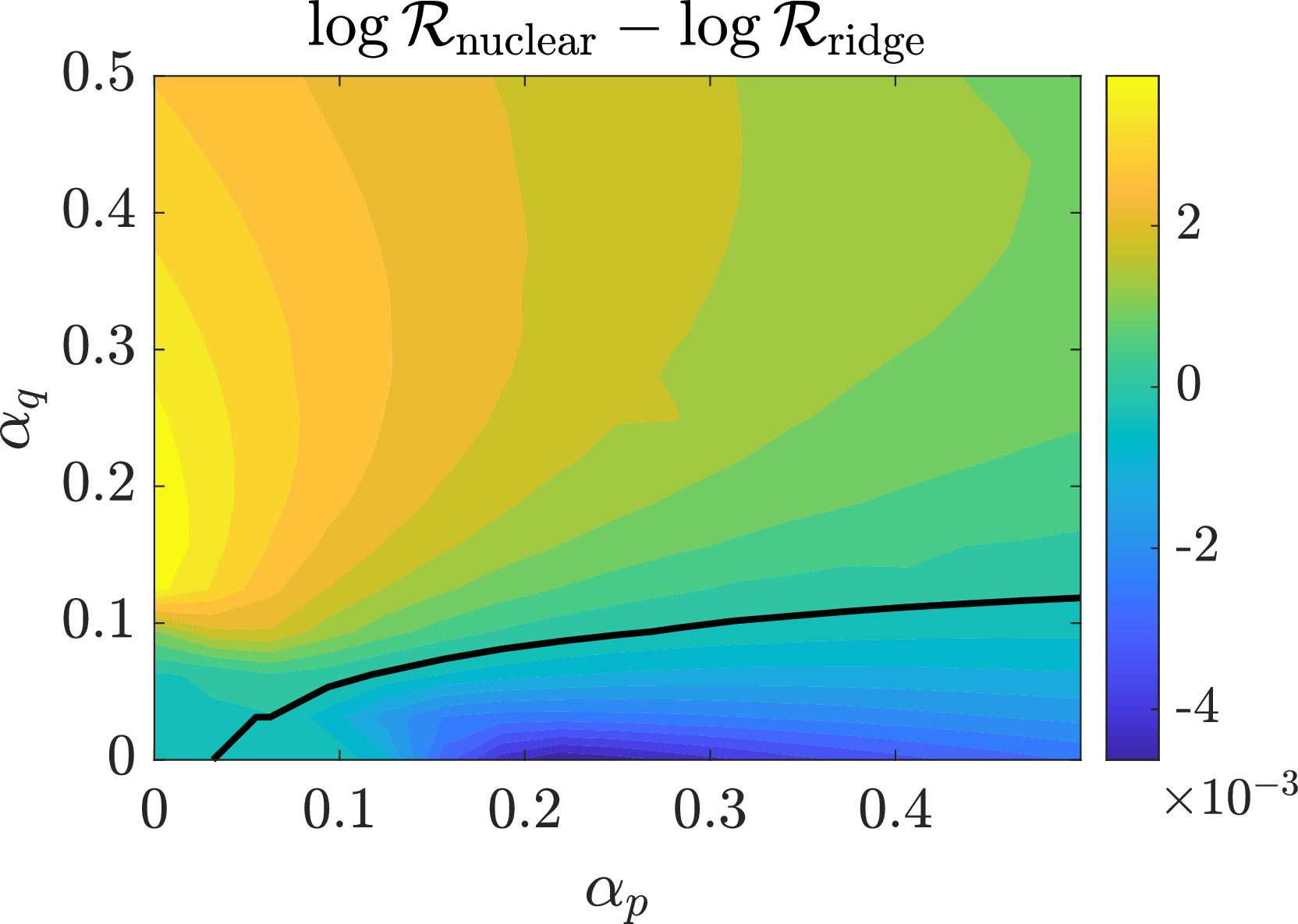
References↩︎
Note that the affine invariance allows this simple reparameterization for unregularized estimation, while for regularized estimation, this is a modeling choice.↩︎
In this paper, unless otherwise specified when ambiguous, \(\mathbb{E}_p[ H(x)]\) is the expectation of \(H(x)\) for \(x\) distributed as \(p\).↩︎
These limits are immediate consequences of the law of large numbers for chi-square variables and standard Gaussian concentration [29]. Indeed, \(\hat{\mu}_p=\Delta+n_p^{-1/2}G_p\) and \(\hat{\mu}_q=n_q^{-1/2}G_q\), with independent standard Gaussian vectors \(G_p,G_q\in\mathbb{R}^m\). Hence \(\|\hat{\mu}_p\|^2=s+2n_p^{-1/2}\Delta^\top G_p+n_p^{-1}\|G_p\|^2\to s+\alpha_p,\) because \(n_p^{-1/2}\Delta^\top G_p\to0\) in probability and \(n_p^{-1}\|G_p\|^2=(m/n_p)(m^{-1}\|G_p\|^2)\to\alpha_p\). The proof for \(\hat{\Delta}\) is identical, with noise covariance matrix \((n_p^{-1}+n_q^{-1})I= (\alpha_p + \alpha_q) \frac{1}{m} I\).↩︎
The MATLAB code for all figures in this paper can be found at https://www.di.ens.fr/~fbach/fdiv_gaussian.zip.↩︎