C2E: Boosting Ego-Only 3D Object Detection via Multi-Teacher Contrastive Knowledge Distillation
July 02, 2026
Abstract
LiDAR-based 3D object detection is essential for autonomous driving systems. However, traditional Ego-only Perception (Eo-Perception) suffers from limited perspective and occlusions in a complex outdoor environment, leading to performance bottlenecks. Recently, research on multi-agent Collaborative Perception (Co-Perception) has demonstrated excellent performance, but high communication costs and accumulated pose error hinder its application. To address this, we explore a novel C2E (Co-Perception to Eo-Perception) paradigm through the Multi-to-Single (M2S) agent contrastive knowledge distillation framework. Our M2S framework first designs Multi-Level Feature Enhancement module to provide more stable features, and introduces Auxiliary Point Cloud Reconstruction and Multi-Teacher Contrastive Distillation mechanisms to mitigate domain gaps in point cloud and feature distributions within the C2E paradigm. Benefiting from this, our M2S can retain the excellent performance of collaborative perception while effectively avoiding the drawbacks, such as communication delays and positioning errors. Extensive experiments on the V2XSet, V2V4Real and DAIR-V2X datasets show the effectiveness and generalizability of our M2S framework when combined with the state-of-the-art CoSDH model and other excellent 3D detectors. Our M2S framework can deliver up to a 8.64% improvement in 3D mAP performance without introducing any communication costs.
1 Introduction↩︎
3D object detection is a crucial task for autonomous driving and other unmanned systems [1]–[3]. Recently, LiDAR-based methods have achieved remarkable progress [4], [5] and have been widely adopted, owing to the precise spatial information provided by LiDAR sensors [6].
Outdoor environments, however, present complex and dynamic challenges, including diverse occlusions and extreme long-range detection requirements. These factors significantly impact Ego-only Perception (Eo-Perception), leading to inaccurate perception results [7], [8]. While previous research [9]–[13] has attempted to alleviate these challenges of Eo-Perception by using more information or multi-sensor distillation, a noticeable performance bottleneck remains.
Recently, some efforts have been made to investigate Collaborative Perception (Co-Perception), such as vehicle-to-vehicle (V2V), vehicle-to-infrastructure (V2I), and vehicle-to-everything (V2X) [14]–[17]. Leveraging shared information among agents has demonstrated outstanding performance in the domain of cooperative 3D object detection. Nonetheless, the collaborative challenges that arise in real-world scenarios, such as high communication costs and localization errors, continue to hinder its real-world applications significantly.
Consequently, several existing methods have attempted to address the collaboration challenges by studying how, when, and where to communicate or by compressing communication features [18]–[22]. Nevertheless, despite some progress, these collaboration challenges still hinder the practical application of collaborative 3D object detection, primarily due to the restrictive nature of the existing collaboration mechanisms [23].
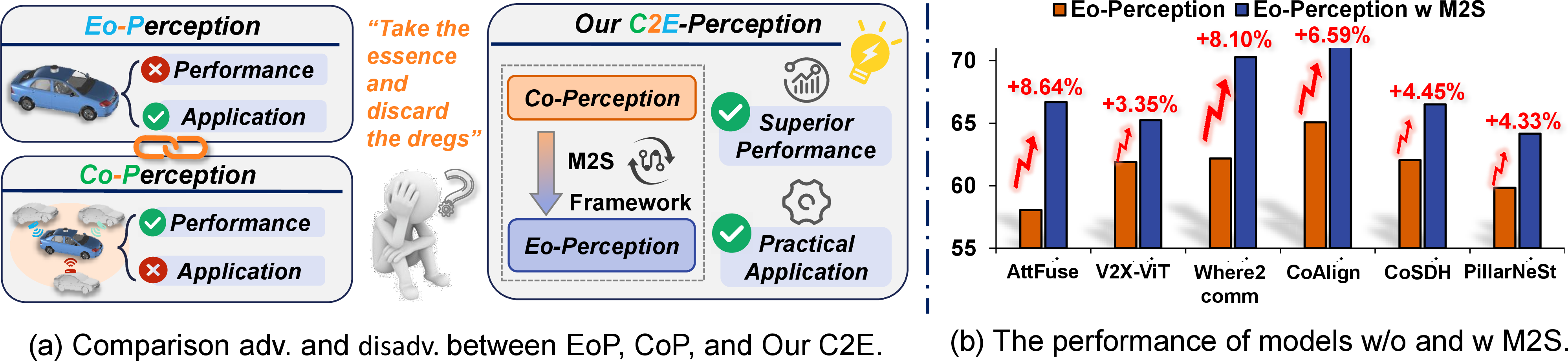
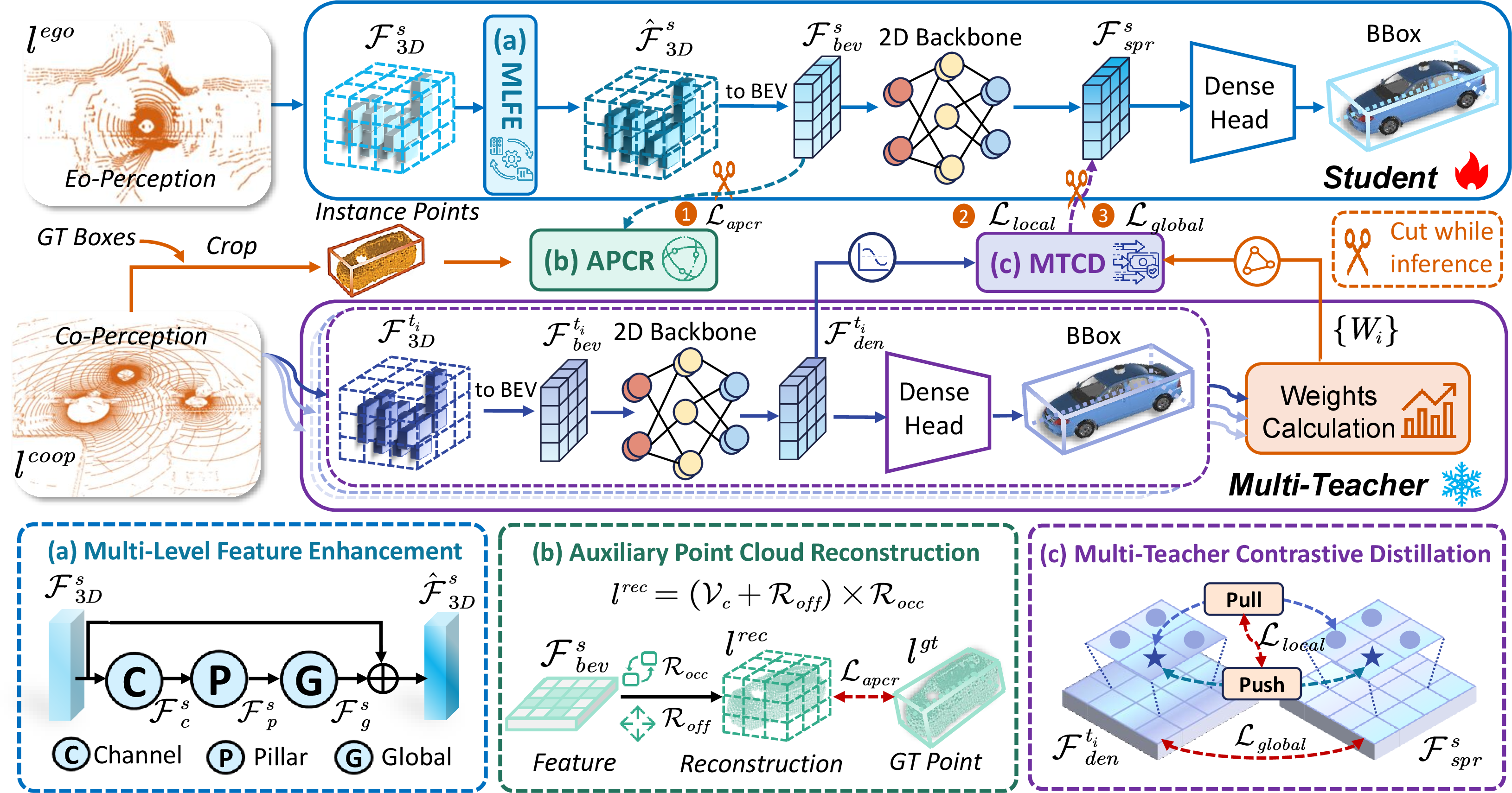
Based on existing research, we have summarized the strengths and weaknesses of these two perception paradigms. As illustrated in Fig. 1 (a), Eo-Perception is practical but has performance bottlenecks, whereas Co-Perception delivers superior performance while encountering collaboration challenges. "Take the essence and discard the dregs." Can the advantages of both be combined? This is the core question this paper addresses. To this end, we explore a novel perception paradigm, C2E-Perception: transferring the superior performance of Co-Perception to practical Eo-Perception. Specifically, at the training stage, we retain high-density information and collaborative knowledge from the Co-Perception teacher to the Eo-Perception student through the knowledge distillation technique. At the inference stage, we use the Eo-Perception student for individual inference to mitigate collaboration challenges.
However, simple knowledge distillation faces substantial domain gaps in data and feature distributions between single-agent and multi-agent data, which limits the effective transfer of collaborative perception knowledge. To bridge these gaps, we introduce the Auxiliary Point Cloud Reconstruction (APCR) and Multi-Teacher Contrastive Distillation (MTCD) strategies to mitigate the significant discrepancy in data and feature distributions, respectively. Moreover, to provide more stable features for distillation, we propose Multi-Level Feature Enhancement (MLFE) to enhance the feature extraction capability of the student.
As shown in Fig. 1 (b), extensive experiments conducted on both real-world and simulated datasets demonstrate the effectiveness and generalizability of our M2S framework when integrated with the state-of-the-art model [24] and other excellent 3D detectors. In summary, our main contributions are as follows.
To the best of our knowledge, we are the first to explore the Co-Perception to Eo-Perception (C2E-Perception) paradigm. We propose the novel M2S framework based on multi-teacher adaptive contrastive knowledge distillation.
We effectively mitigate the significant data and feature gaps between multi-agent and single-agent domain through Auxiliary Point Cloud Reconstruction (APCR) and Multi-Teacher Contrastive Distillation (MTCD). Moreover, we use the Multi-Level Feature Enhancement (MLFE) to provide more stable features for distillation.
Extensive experiments on the V2XSet, V2V4Real, and DAIR-V2X datasets validate the effectiveness of the proposed M2S framework. Our M2S framework can deliver an improvement of up to 8.64 in 3D mAP performance without introducing any communication costs.
2 Related work↩︎
3D Object Detection for Single Agent. 3D object detection aims to identify object categories and spatial locations from sparse and irregular point clouds. Existing single-agent methods fall into three categories: point-based [25], [26], grid-based [2], [27]–[29], and point-voxel hybrid approaches [30], [31]. However, single-agent systems rely solely on onboard sensors, resulting in limited perception angles and susceptibility to occlusions, blind spots, and complex traffic dynamics [8]. Furthermore, the limited sensing range constrains distant object detection [23], causing performance bottlenecks in high-speed or sparse scenes.
Collaborative Perception for Multi-Agents. Collaborative perception has been proposed to overcome the limitations of a single viewpoint. Depending on the fusion stage, it can be categorized into early [32]–[34], intermediate [14]–[16], [24], [35], and late fusion [36], [37]. Despite its advantages, collaborative perception faces challenges such as high bandwidth demands for feature or raw data transmission [38] and accumulated errors from inaccurate relative pose estimation [22], [23]. DiscoNet [32] reduces communication costs via a distilled graph; V2X-INCOP [39] improves fault tolerance under interruptions, yet both remain in the collaborative paradigm with latency and infrastructure constraints. Thus, improving perception performance while reducing communication overhead remains a key research focus.
3D Object Detection Based on Knowledge Distillation. Knowledge distillation has been applied to 3D object detection [9], [11], [40] and recent collaborative perception [32], [41]. Multi-teacher schemes yield richer knowledge than single-teacher ones; MKD-Cooper [42] exploits this for robustness. Unlike [43], which refines other agents’ predictions as pseudo-labels, our method distills collaborative knowledge directly into the ego model. We thus propose M2S, a multi-teacher adaptive contrastive distillation framework that transfers dense knowledge from multiple teachers to a sparse student.
3 Methodology↩︎
3.1 Problem Statement and Overall Design↩︎
Problem Statement. In collaborative perception based on V2X communication, there are three types of agents: Ego, Connected Automated Vehicles (CAVs), and Infrastructure units (Inf). In our proposed framework, the collaborative perception (Co-Perception) teacher detector \(\mathcal{D}^{t}\) receives lidar point cloud input \(l^{coop} = \{l^{ego}, l^{cav}, l^{Inf}\}\) from all agents. In contrast, the ego-only perception (Eo-Perception) student detector \(\mathcal{D}^{s}\) only takes point cloud data \(\{l^{ego}\}\) from the ego vehicle, thus enabling single-agent 3D object detection. The goal of 3D object detection is to regress a set of 3D bounding boxes \(\mathcal{B} = \{b_i\}_{i=1}^{N_b}\), where \(\mathcal{B} \in \mathbb{R}^{N_b \times 7}\) and \(N_b\) denotes the number of predicted bounding boxes.
Overall Design. Due to the varying number of participating agents, large gaps exist between \(\mathcal{D}^{t}\) and \(\mathcal{D}^{s}\) in both feature representation and point cloud domains. To address this challenge, we propose a Multi-to-Single (M2S) agent contrastive knowledge distillation framework, as illustrated in Fig. 2. First, the Multi-Level Feature Enhancement (MLFE) module (Fig. 2 (a)) progressively enhances 3D features in \(\mathcal{D}^{s}\) across multiple levels and dimensions. Then, the Auxiliary Point Cloud Reconstruction (APCR) module (Fig. 2 (b)) encourages the student to learn point cloud distributions consistent with \(\mathcal{D}^{t}\). Finally, the Multi-Teacher Contrastive Distillation (MTCD) strategy (Fig. 2 (c)) transfers locally structured and globally salient features from the teacher model to the student via contrastive learning and adaptive weighting, which further mitigates the feature disparity between \(\mathcal{D}^{t}\) and \(\mathcal{D}^{s}\). Note that only the student detector \(\mathcal{D}^{s}\) is used during inference.
We provide the formal definitions of the three paradigms in the Appx. and the following sections provide detailed descriptions of each module.
3.2 Multi-Level Feature Enhancement↩︎
In the teacher \(\mathcal{D}^{t}\), the ego vehicle obtains high-density features through communication with other agents. In contrast, the student \(\mathcal{D}^{s}\) relies solely on its own sensors, producing relatively sparse features that limit 3D detection performance. To enhance the feature extraction capability of \(\mathcal{D}^{s}\) and provide stable features for distillation, we propose the Multi-Level Feature Enhancement (MLFE) module, which progressively refines 3D features \(\mathcal{F}_{3D}^{s}\) from local to global levels.
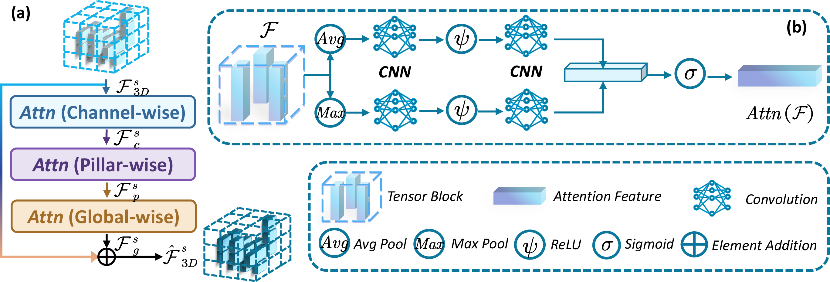
As shown in Fig. 3, MLFE enhances the student’s 3D features along three dimensions: Channel, Pillar, and Global, through hierarchical attention mechanisms. The student detector \(\mathcal{D}^{s}\) receives a 3D feature tensor \(\mathcal{F}_{3D}^{s} \in \mathbb{R}^{C \times P \times G}\), where \(C\), \(P\) and \(G\) denote channels, points per pillar, and the numbers of global pillars, respectively. By progressively re-weighing semantic channels, reinforcing local geometric consistency, and integrating global contextual information, MLFE enhances students’ representational capabilities, thereby generating more robust and domain-invariant features for distillation.
Inspired by SCNet3D [44] and CBAM [45], MLFE applies feature weight calculation (\(Attn\)) to generate three attention maps: \[\begin{align} Attn(\mathcal{F}) &= \sigma ( \delta ( \psi \left( \delta \left(\theta_{max}(\mathcal{F}) \right) \right) \\ & + \delta \left( \psi\left( \delta \left( \theta_{avg}(\mathcal{F}) \right) \right) \right), \end{align}\] where \(\theta_{max}\) and \(\theta_{avg}\) denote max_pooling and average_pooling, \(\delta\) denotes convolution, \(\psi\) denotes ReLU activation, and \(\sigma\) denotes sigmoid activation.
Then, we apply \(Attn\) to \(\mathcal{F}_{3D}^{s}\) along the channel, pillar, and global dimensions sequentially to compute the attention map and refine features step-by-step as:
\[\begin{align} \mathcal{F}_{c}^{s}=\mathcal{F}_{3D}^{s} \otimes Attn(\mathcal{F}_{3D}^{s}) \oplus \mathcal{F}_{3D}^{s}, \\\mathcal{F}_{p}^{s}=\mathcal{F}_{c}^{s} \otimes Attn(\mathcal{F}_{c}^{s}) \oplus \mathcal{F}_{c}^{s} , \\\mathcal{F}_{g}^{s}=\mathcal{F}_{p}^{s} \otimes Attn(\mathcal{F}_{p}^{s}) \oplus \mathcal{F}_{p}^{s}, \\ \enspace\mathrm{and } \enspace \hat{\mathcal{F}}_{3D}^{s} =\mathcal{F}_{3D}^{s} \oplus \mathcal{F}_{g}^{s}, \end{align}\] where \(\otimes\) indicates element-wise multiplication and \(\oplus\) denotes element-wise addition. The final output \(\hat{\mathcal{F}}_{3D}^{s}\) integrates attention-weighted 3D feature along all dimensions.
3.3 Auxiliary Point Cloud Reconstruction↩︎
The teacher detectors \(\mathcal{D}^{t}\) receives dense point cloud input \(l^{coop}\) from multi-agent cooperation, while the student \(\mathcal{D}^{s}\) only processes a sparse ego point cloud \(l^{ego}\). This leads to a clear disparity in the point cloud distribution domains between the two networks. To address this gap, we introduce an Auxiliary Point Cloud Reconstruction module (APCR) for the student model during the training phase. Unlike prior works [46]–[48], which focus on scene-level reconstruction, our method performs instance-level reconstruction between teacher and student. Specifically, we extract point clouds within ground-truth bounding boxes and re-voxelize them as supervision targets.
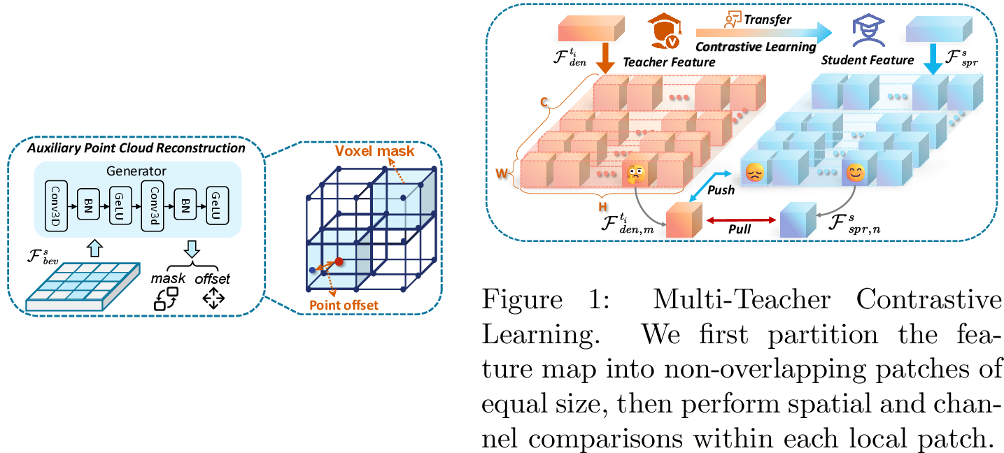
Since directly recovering dense point clouds incurs substantial computational and memory overhead, inspired by [46], we decompose the auxiliary point cloud reconstruction task into two sub-tasks: voxel occupancy mask \(\mathcal{R}_{occ}\) prediction and point offset \(\mathcal{R}_{off}\) estimation. As illustrated in the Fig. 4, APCR first performs dimensionality expansion on the 2D feature \(\mathcal{F}_{bev}^{s}\), projecting it back into 3D space, and then processes it through multiple layers of \(1 \times 1\) 3D convolution with GELU activation to generate \(\mathcal{R}_{occ}\) and \(\mathcal{R}_{off}\).
Thus, the reconstructed point cloud can be calculated as: \[\begin{align} l^{rec} = (\mathcal{V}_{c} + \mathcal{R}_{off}) \times \mathcal{R}_{occ}, \end{align}\] where \(l^{rec}\) is the reconstructed dense point cloud and \(\mathcal{V}_{c}\) denotes to the center of voxel.
We supervise the voxel occupancy prediction mask using a binary cross-entropy \(H\) loss, and the point offset estimation using an L1 regression loss. They are defined as: \[\begin{align} \mathcal{L}_{occ} &= -\frac{N_{bg}}{N_{fg}} \, H(\mathcal{G}_{occ}, \mathcal{P}_{occ}), \\ \mathcal{L}_{off} &= \frac{1}{|N_{fg}|} \sum_{i=1}^{N_{fg}} \| (\mathcal{V}_{c_i} + \mathcal{R}_{off_i}) - O_{gt_i} \| , \end{align}\] where \(\mathcal{G}_{occ}\) denotes the ground-truth occupancy annotation and \(\mathcal{P}_{occ}\) denotes the predicted occupancy probability; \(N_{fg}\) and \(N_{bg}\) are the numbers of foreground and background voxels; \(O_{gt_i}\) represents the ground-truth point cloud of the \(i\)-th foreground voxel.
The final reconstruction loss is the sum of occupancy loss and offset loss: \[\begin{align} \mathcal{L}_{apcr} = \mathcal{L}_{occ} + \mathcal{L}_{off} . \end{align}\]
3.4 Multi-Teacher Contrastive Distillation↩︎
Multi-agent teachers contain richer contextual and structural knowledge, while the student’s single-view limitation creates a feature gap that hinders the direct acquisition of such dense features. To bridge this gap and effectively transfer locally structured and globally salient features from teacher detectors \(\mathcal{D}^{t}\) to the target student model \(\mathcal{D}^{s}\), we propose the Multi-Teacher Contrastive Distillation (MTCD) strategy.
As shown in Fig. [mtcl], we partition each BEV feature map into multiple non-overlapping regions, which are treated as contrastive samples. Unlike label-based contrastive frameworks [49], the positive and negative pairs are constructed within teacher–student feature correspondences \((\mathcal{F}_{den}^{t}, \mathcal{F}_{spr}^{s})\), based on their spatial alignment. Formally, a positive pair is defined for identical spatial indices \((m = n)\) between \((\mathcal{F}_{spr,m}^{s}, \mathcal{F}_{den,n}^{t})\), where \(m\) and \(n\) denote the spatial locations on the BEV feature map. Conversely, negative pairs correspond to index mismatches \((m \neq n)\).
The contrastive loss \(\mathcal{L}_{CL}^{t_i}\) for the \(i\)-th teacher is: \[\begin{align} \mathcal{L}_{CL}^{t_i} = \frac{1}{N} \sum_{m=1}^{N} -\log \frac{\exp(-d_{m,m}^{t_i} / \tau)}{ \sum_{n=1}^{N} \mathbb{1}_{m \neq n} \exp(-d_{m,n}^{t_i} / \tau)}, \end{align}\] Where \(\tau = 0.07\) is the temperature parameter, \(N\) denotes the number of contrastive pairs, and \(\mathbb{1}_{m \neq n}\) is an indicator function that equals 1 only when \(m \neq n\). The feature similarity is measured using the squared Euclidean distance: \(d_{m,m}^{t_i} = \|\mathcal{F}_{spr,m}^{s}- \mathcal{F}_{den,m}^{t_i}\|_2^2\) and \(d_{m,n}^{t_i} = \|\mathcal{F}_{spr,m}^{s}- \mathcal{F}_{den,n}^{t_i}\|_2^2\) .
To enable the student to capture the teacher’s locally dense and structured knowledge by focusing on contextual cues and position–channel group information, we combine two complementary contrastive modes: Spatial Contrasting and Channel Contrasting. The detailed formulation is provided in the Appx..
Accordingly, we use \(\mathcal{L}_{local}\) to emphasize fine-grained local structural alignment, which is defined as: \[\begin{align} \mathcal{L}_{local} = \sum_{i=1}^{T} W_i \cdot \mathcal{L}_{CL}^{t_i}, \end{align}\] where \(W_i\) is the confidence weight for the \(i\)-th teacher, based on multi-teacher adaptive distillation mechanism.
Multi-Teacher Adaptive Distillation. Due to variations in perceptual capabilities across different teacher models under diverse scenarios or samples, direct averaging fusion may introduce noise or even misguide training. To achieve high-quality knowledge transfer, we further designed a Multi-Teacher Adaptive Distillation mechanism. This design dynamically assigns weights based on the teacher model’s performance on the current sample.
Specifically, we use the localization loss of 3D bounding box prediction as the performance indicator. For the \(i\)-th teacher, the localization loss \(\mathcal{L}_{loc}^{t_i}\) is computed by Smooth \(L_1\) loss between the predicted box \(\mathcal{\hat{B}}_{t_i}\) and the ground truth \(\mathcal{B}_{gt}\): \(\mathcal{L}_{loc}^{t_i} = \text{Smooth}_{L_1} \left( \mathcal{\hat{B}}_{t_i}, \mathcal{B}_{gt} \right).\)
Then, the confidence weight \(W_i\) is obtained by the localization loss across all teachers: \[W_i = \frac{\exp(-\alpha \cdot \mathcal{L}_{loc}^{t_i})}{\sum_{j=1}^{T} \exp(-\alpha \cdot \mathcal{L}_{loc}^{t_j})}, \label{eq:weight}\tag{1}\] where \(\alpha=0.8\) is a scaling factor that controls the sensitivity of the confidence to the loss. This weighting scheme prioritizes teachers with higher confidence.
Moreover, to further guide the student \(\mathcal{D}^s\) to approximate the comprehensive dense BEV feature \(\hat{\mathcal{F}}_{den,k}^{t}\) of teachers \(\mathcal{D}^t\) in global level, we employ a multi-teacher adaptive distillation approach. Specially, we consider \(T\) pre-trained teacher models \(\mathcal{D}^{t_i}\), which generate dense features. For the \(k\)-th layer, let \(\mathcal{F}_{den,k}^{t_i} = \mathcal{D}^{t_i}(l^{coop})\) denote the dense BEV features of the \(i\)-th teacher. We fused these features into \(\hat{\mathcal{F}}_{den,k}^{t}\) by: \[\hat{\mathcal{F}}_{den,k}^{t} = \sum_{i=1}^{T} W_i \cdot \mathcal{F}_{den,k}^{t_i}, \label{eq:fusion}\tag{2}\] where \(W_i\) is the confidence weight for the \(i\)-th teacher, which is computed based on the detection performance of the teacher.
Finally, we employ KL-divergence feature distillation as: \[\mathcal{L}_{global} = \sum_{k=1}^K \beta^k_{kd} \cdot \mathcal{D}_{KL} \left( \rho(\mathcal{F}^{s}_{spr,k}) \parallel \rho(\hat{\mathcal{F}}_{den,k}^{t}) \right), \label{eq:feature95distill}\tag{3}\] where \(\rho\) denotes softmax function, and \(\mathcal{D}_{\mathrm{KL}}(\pi \| p) = \mathbb{E}_{\pi(x)} [ \log \frac{\pi(x)}{p(x)} ]\) is the Kullback-Leibler divergence, and the hyperparameter \(\beta_{kd}^k \in \{0.2,0.3,0.5 \}\) to balance weights across different feature layers, which set same to [42].
3.5 Loss Function↩︎
We train our M2S using the following loss function: \[\begin{align} \mathcal{L}_{M2S} = \gamma_{cls} \mathcal{L}_{cls} + \gamma_{loc} \mathcal{L}_{loc} + \gamma_{apcr} \mathcal{L}_{apcr}\\ + \gamma_{global} \mathcal{L}_{global} + \gamma_{local} \mathcal{L}_{local}, \end{align}\] where the hyperparameters \(\gamma_{cls}\), \(\gamma_{loc}\), \(\gamma_{apcr}\), \(\gamma_{global}\) and \(\gamma_{local}\) balance the contributions of different losses, and \(\mathcal{L}_{cls}\) denotes the classification loss implemented with focal loss, \(\mathcal{L}_{loc}\) represents the bbox regression loss using Smooth \(L_1\).
4 Experiments↩︎
4.1 Datasets and Evaluation Metrics↩︎
Datasets. We conduct comprehensive experiments on two large-scale real-world datasets, V2V4Real [50] and DAIR-V2X [51], as well as a simulated dataset, V2XSet [14]. We provide more datasets information in the Appx..
Evaluation Metrics. We adopt the average precision (AP) as the main indicators for evaluating 3D object detection performance. Additionally, we record the delay and frames per second (FPS) to measure the communication latency and inference efficiency, respectively. And we report the number of floating-point operations (FLOPs) to assess the computational complexity during inference. Furthermore, we use single NVIDIA RTX 3090 GPU to report training time (hours) and GPU memory usage (MB) and discuss the training cost.
| Models | Publication | 3D mAP\(@\)Validation | 3D mAP\(@\)Testing | ||||
| IoU=0.3 | IoU=0.5 | IoU=0.7 | IoU=0.3 | IoU=0.5 | IoU=0.7 | ||
| 1.AttFuse | ICRA 2022 | 78.89 | 76.72 | 68.10 | 75.67 | 73.72 | 58.06 |
| 2.AttFuse w/ M2S | 85.20 | 82.83 | 73.73 | 82.15 | 79.26 | 66.70 | |
| Improvement (2-1) | +6.31 | +6.11 | +5.63 | +6.48 | +5.54 | +8.64 | |
| 1.V2X-ViT | ECCV 2022 | 78.20 | 76.84 | 67.51 | 78.86 | 76.17 | 61.90 |
| 2.V2X-ViT w/ M2S | 83.97 | 82.45 | 72.49 | 83.91 | 81.02 | 65.25 | |
| Improvement (2-1) | +5.77 | +5.61 | +4.98 | +5.05 | +4.85 | +3.35 | |
| 1.Where2comm | NeurIPS 2022 | 80.22 | 78.23 | 68.44 | 79.21 | 76.24 | 62.18 |
| 2.Where2comm w/ M2S | 84.99 | 83.26 | 75.15 | 84.42 | 82.32 | 70.28 | |
| Improvement (2-1) | +4.77 | +5.03 | +6.71 | +5.21 | +6.08 | +8.10 | |
| 1.CoAlign | ICRA 2023 | 80.60 | 78.63 | 69.74 | 80.62 | 78.02 | 65.07 |
| 2.CoAlign w/ M2S | 88.11 | 86.27 | 77.15 | 86.49 | 83.88 | 71.66 | |
| Improvement (2-1) | +7.51 | +7.64 | +7.41 | +5.87 | +5.86 | +6.59 | |
| 1.CoSDH | CVPR 2025 | 80.74 | 78.53 | 67.91 | 79.52 | 76.75 | 62.05 |
| 2.CoSDH w/ M2S | 87.00 | 84.18 | 75.13 | 84.81 | 81.39 | 66.50 | |
| Improvement (2-1) | +6.26 | +5.65 | +7.22 | +5.29 | +4.64 | +4.45 | |
| 1.PillarNeSt | TIV 2024 | 79.14 | 77.66 | 67.85 | 77.05 | 74.29 | 59.83 |
| 2.PillarNeSt w/ M2S | 85.94 | 84.09 | 71.82 | 84.14 | 81.53 | 64.16 | |
| Improvement (2-1) | +6.80 | +6.43 | +3.97 | +7.09 | +7.24 | +4.33 | |
0.6pt
4.2 Baselines Selection and Experimental Details↩︎
Baselines Selection. We use traditional ego-only methods, for instance, PillarNeSt [52] to validate our M2S framework and also run the collaborative baselines, including AttFuse [15], V2X-ViT [14], Where2comm [20], CoAlign [22], and CoSDH [24], with ego-only input to examine performance in realistic ego-only perception scenarios. Overall, our experimental setup was designed to fully validate the performance of our M2S across different perception methods.
Experimental Details. We use the ego agent for evaluation, following the settings of [15]. We employ three pre-trained models as teachers: AttFuse [15], V2X-ViT [14], and CoSDH [24]. We implement a teacher network that receives only the multi-agent input and a student network that receives only the ego-agent input. During training, the student network is constructed following the full collaborative architecture, including the fusion modules, but receives only the ego-agent input. During inference, only the student detector, which takes only the ego-agent input, is used for prediction to ensure a fair comparison. We provide more experimental details in the Appx..
4.3 Performance Evaluation↩︎
Results on the V2XSet dataset. Table 1 compares several baselines with our M2S framework. Both the collaborative perception methods and ego-only perception method [52] baselines exhibit clear performance gains with our M2S. Notably, on the test set, M2S improves 3D mAP (IoU\(=\)0.7) by 8.64%, 3.35%, 8.10%, 6.59%, 4.45%, and 4.33% for AttFuse [15], V2X-ViT [14], Where2comm [20], CoAlign [22], CoSDH [24], and PillarNeSt [52], respectively. Most importantly, these gains are achieved with no extra communication overhead, validating our M2S’s effectiveness and practicality.
| Models | V2V4Real Val | V2V4Real Test | DAIR-V2X Val | |||||||
| AP\(@\)0.3 | AP\(@\)0.5 | AP\(@\)0.7 | AP\(@\)0.3 | AP\(@\)0.5 | AP\(@\)0.7 | AP\(@\)0.3 | AP\(@\)0.5 | AP\(@\)0.7 | ||
| 1.AttFuse | 49.22 | 44.80 | 25.69 | 44.64 | 40.66 | 21.49 | 58.97 | 49.70 | 33.25 | |
| 2.AttFuse w/ M2S | 57.16 | 47.44 | 26.57 | 53.85 | 45.76 | 26.88 | 61.02 | 52.16 | 39.86 | |
| Improvement (2-1) | +7.94 | +2.64 | +0.88 | +9.21 | +5.10 | +5.39 | +2.05 | +2.46 | +6.61 | |
| 1.V2X-ViT | 52.00 | 46.98 | 25.30 | 46.59 | 41.40 | 19.56 | 60.71 | 51.06 | 35.08 | |
| 2.V2X-ViT w/ M2S | 58.78 | 47.44 | 26.77 | 54.66 | 44.49 | 20.85 | 60.65 | 52.77 | 39.77 | |
| Improvement (2-1) | +6.78 | +0.46 | +1.47 | +8.07 | +3.09 | +1.29 | +1.71 | +4.69 | ||
| 1.Where2comm | 46.80 | 43.57 | 27.03 | 47.33 | 42.08 | 25.17 | 59.42 | 51.10 | 38.54 | |
| 2.Where2comm w/ M2S | 57.04 | 44.72 | 25.55 | 55.50 | 47.07 | 26.79 | 60.84 | 52.24 | 39.84 | |
| Improvement (2-1) | +10.24 | +1.15 | +8.17 | +4.99 | +1.62 | +1.42 | +1.14 | +1.30 | ||
| 1.CoAlign | 46.67 | 41.75 | 23.77 | 48.54 | 40.94 | 21.48 | 61.26 | 51.26 | 37.86 | |
| 2.CoAlign w/ M2S | 55.16 | 45.45 | 24.13 | 54.27 | 46.84 | 23.74 | 62.77 | 53.14 | 38.75 | |
| Improvement (2-1) | +8.49 | +3.70 | +0.36 | +5.73 | +5.90 | +2.26 | +1.51 | +1.94 | +0.95 | |
| 1.CoSDH | 46.04 | 42.85 | 25.07 | 46.79 | 43.20 | 23.11 | 57.50 | 48.57 | 34.37 | |
| 2.CoSDH w/ M2S | 55.98 | 46.25 | 24.42 | 56.54 | 47.91 | 25.53 | 60.19 | 51.67 | 37.33 | |
| Improvement (2-1) | +9.94 | +3.40 | +9.75 | +4.71 | +2.42 | +2.69 | +3.10 | +2.96 | ||
| 1.PillarNeSt | 50.61 | 45.36 | 21.70 | 47.90 | 40.20 | 16.18 | 57.30 | 48.90 | 33.46 | |
| 2.PillarNeSt w/ M2S | 52.19 | 45.28 | 26.03 | 53.99 | 43.55 | 25.24 | 60.36 | 51.85 | 38.17 | |
| Improvement (2-1) | +1.58 | +4.33 | +6.09 | +3.35 | +9.06 | +3.06 | +2.95 | +4.71 | ||
0.6pt
Results on the real-world datasets. To further verify the effectiveness and generalization of our M2S in real-world scenarios, we conduct experiments on V2V4Real [50] and DAIR-V2X [51]. As with V2XSet [14], both collaborative [14], [15], [20], [22], [24] and ego-only [52] baselines gain consistently. Specifically, On V2V4Real test set at AP\(@\)0.7, all baselines consistently improve with M2S, with PillarNeSt achieving the largest gain of \(9.06\), followed by AttFuse (\(+5.39\)), CoSDH (\(+2.42\)), and CoAlign (\(+2.26\)). A similar trend is observed on the DAIR-V2X, where M2S consistently enhances performance across multiple models, confirming its robustness across diverse environments.
| Row | Module | Validation | Testing | ||||||||
| ST | MTCD\(^\dagger\) | MLFE | APCR | MTCD\(^\ddagger\) | AP\(@\)0.3 | AP\(@\)0.5 | AP\(@\)0.7 | AP\(@\)0.3 | AP\(@\)0.5 | AP\(@\)0.7 | |
| 1 | - | - | - | - | - | 78.89 | 76.72 | 68.10 | 75.67 | 73.72 | 58.06 |
| 2 | \(✔\) | - | - | - | - | 82.83 | 80.17 | 68.54 | 78.10 | 74.77 | 58.29 |
| 3 | - | \(✔\) | - | - | - | 84.10 | 81.91 | 71.64 | 81.98 | 78.55 | 62.76 |
| 4 | - | \(✔\) | \(✔\) | - | - | 84.31 | 82.27 | 72.85 | 82.15 | 79.44 | 64.58 |
| 5 | - | \(✔\) | \(✔\) | \(✔\) | - | 84.91 | 82.75 | 73.08 | 81.80 | 79.32 | 66.50 |
| 6 | - | \(✔\) | \(✔\) | \(✔\) | \(✔\) | 85.20 | 82.83 | 73.73 | 82.15 | 79.26 | 66.70 |
4.4 Ablation Study↩︎
Table 3 ablates each module in M2S. We adopt AttFuse [15], V2X-ViT [14], and CoSDH [24] as teacher models, with AttFuse that receives single-agent input as the student. Introducing single-teacher distillation (ST) alone yields a slight improvement in AP\(@\)0.7 from 58.06% to 58.29%. Replacing it with the multi-teacher adaptive distillation module (row 3) significantly boosts performance to 62.76%, demonstrating the benefit of leveraging multiple teachers. Adding the multi-level feature enhancement (MLFE) and auxiliary point cloud reconstruction (APCR) modules further increases AP\(@\)0.7 to 66.50%. Finally, incorporating multi-teacher contrastive learning (row 6) achieves the best result of 66.70%, confirming the complementary effectiveness of all components in M2S.
4.5 Analysis Experiments↩︎
Figure 5: 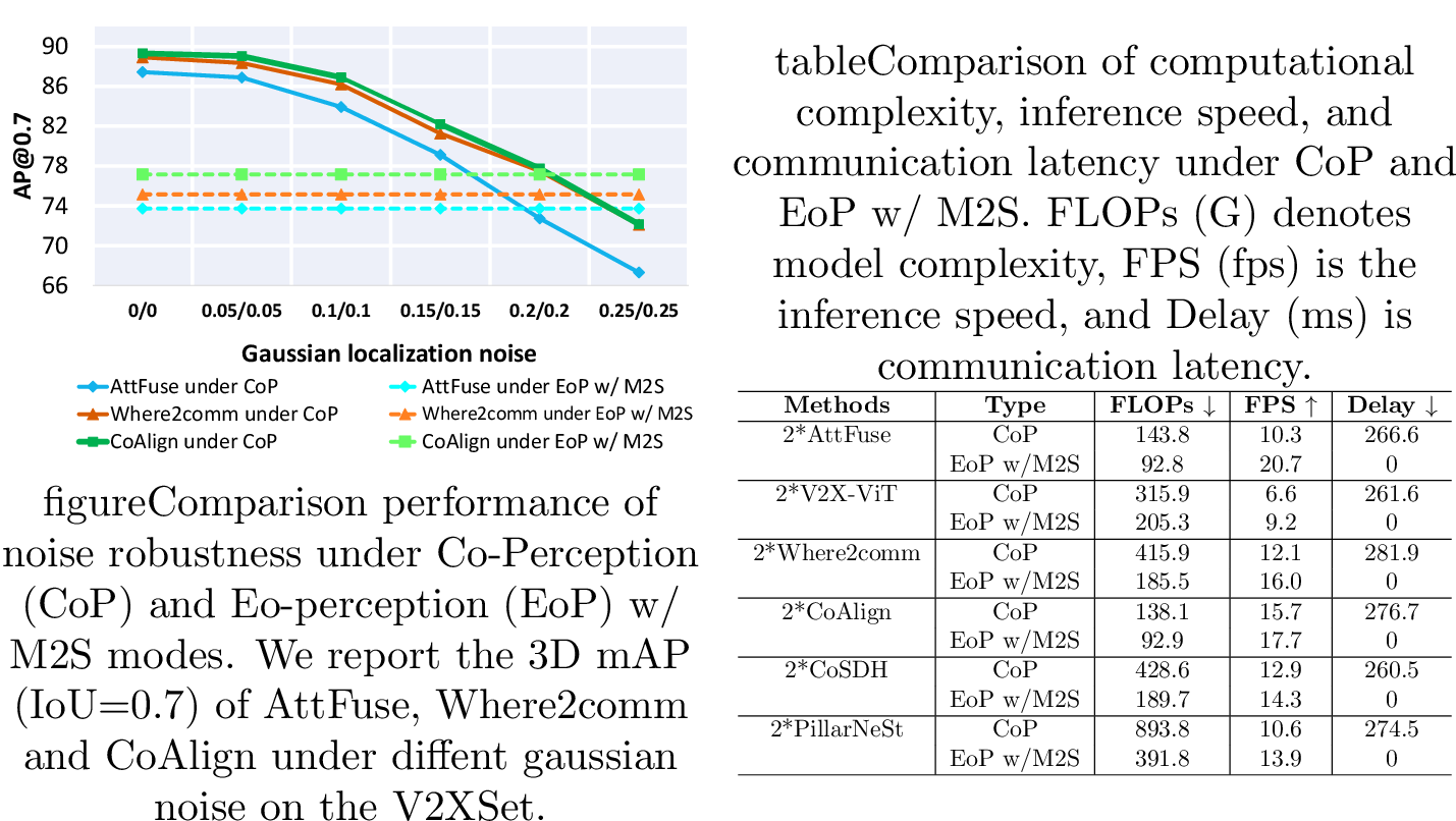 .
.
Comparison of noise robustness. Following the noise injection settings from [20] and [14], we applied Gaussian noise \(\zeta\) from (\(0.0\,\text{m}, 0.0^\circ\)) to (\(0.25\,\text{m}, 0.25^\circ\)) to simulate localization errors under complex scenarios. As shown in Fig. 5, collaborative perception methods suffer severe performance degradation as errors accumulate. In contrast, when the error is within (\(0.25\,\text{m}, 0.25^\circ\)), our M2S maintains consistent performance by relying solely on ego-agent inference, showing that M2S can inherently mitigate the negative impact of localization errors.
Comparison of computational complexity, inference speed, and communication latency. Table [tab:comm] compares Co-Perception (CoP) and Ego-Perception (EoP) with our M2S during inference. The CoP receives multi-agent input, while the EoP only receives the ego. Overall, M2S notably reduces computational complexity, accelerates inference, and eliminates communication latency. Specifically, M2S reduces FLOPs by 35.43% and doubles FPS for AttFuse [15]. Since our M2S does not require external communication, which eliminates transmission delays, whereas collaboration methods suffer from 260 to 282 ms latency. In short, these results confirm M2S’s practicality and deployment potential.
| Teacher Combinations | Performance | Train | GPU | ||
| AP\(@\)0.3 | AP\(@\)0.5 | AP\(@\)0.7 | Time (h) | Mem.(M) | |
| AttFuse (Single teacher) | 84.34 | 82.35 | 73.26 | 7.54 | 7640 |
| AttFuse+CoSDH | 83.95 | 82.20 | 73.69 | 8.05 | 7724 |
| AttFuse+V2X-ViT | 83.74 | 81.45 | 73.41 | 12.13 | 10730 |
| CoSDH+V2X-ViT | 84.25 | 82.74 | 73.30 | 12.10 | 10348 |
| AttFuse+V2X-ViT+CoSDH | 85.20 | 82.83 | 73.73 | 12.69 | 10992 |
| Methods | All Range | Range [0,30) (\(m\)) | Range[30,50) (\(m\)) | Range[50,+inf) (\(m\)) | ||||
| AP\(@\)0.5 | AP\(@\)0.7 | AP\(@\)0.5 | AP\(@\)0.7 | AP\(@\)0.5 | AP\(@\)0.7 | AP\(@\)0.5 | AP\(@\)0.7 | |
| AttFuse | 76.72 | 68.10 | 84.34 | 81.08 | 76.31 | 67.41 | 58.43 | 39.63 |
| AttFuse w/M2S | 82.83 | 73.73 | 95.29 | 92.49 | 78.13 | 68.76 | 60.46 | 39.97 |
| Where2comm | 78.23 | 68.44 | 84.55 | 81.70 | 78.65 | 68.04 | 61.93 | 39.32 |
| Where2comm w/M2S | 83.26 | 75.15 | 95.59 | 93.23 | 78.10 | 69.66 | 62.36 | 42.60 |
| CoAlign | 78.63 | 69.74 | 85.08 | 82.15 | 78.31 | 68.95 | 62.93 | 42.31 |
| CoAlign w/M2S | 86.27 | 77.15 | 96.10 | 93.76 | 80.88 | 72.20 | 71.06 | 48.54 |
0.6pt
Comparison of teacher combinations and discussion of trade-offs. As shown in Table 4, the combination AttFuse+V2X-ViT+CoSDH achieves the highest performance, which comes with substantial training overhead, requiring more training time and higher GPU memory compared to the single-teacher. Notably, other high-cost combinations, like AttFuse+V2X-ViT, fail to deliver comparable accuracy, while the CoSDH+V2X-ViT offers competitive but still inferior results with similar resource consumption. Given its superior accuracy and acceptable training cost, we select AttFuse+V2X-ViT+CoSDH as the final teacher configuration for subsequent experiments.
Comparison of performance across distance ranges. Table 5 shows that integrating M2S consistently improves all methods across all distance ranges. CoAlign achieves the largest overall gain, with AP\(@\)0.7 rising from 69.74 to 77.15. In the short range [0,30), M2S boosts AP\(@\)0.7 by over 10 points for AttFuse, CoAlign, and Where2comm, indicating enhanced local feature modeling. Gains persist in the mid-range [30,50) and extend to the challenging far-range [50,+inf), where CoAlign’s AP\(@\)0.5 increases from 62.93 to 71.06. These results demonstrate M2S’s effectiveness across all distance conditions.
4.6 Qualitative Analysis↩︎
To demonstrate M2S’s efficacy in transferring dense multi-teacher knowledge to sparse students, we show FOV and BEV results on V2XSet with and without M2S in Figs. 6 and [fig:bev]. M2S achieves more comprehensive and precise detection. Without M2S (Eo-Perception alone), students frequently miss or misclassify objects, especially distant or in dense areas. M2S significantly mitigates these issues, effectively distilling collaborative knowledge and enhancing student performance.

5 Conclusion↩︎
In this paper, we analyze the inherent advantages and limitations of Co-Perception and Eo-Perception, and explore the new C2E (Co-Perception to Eo-Perception) paradigm. Through the Multi-to-Single (M2S) agent contrastive knowledge distillation framework, we achieve state-of-the-art performance on 3D object detection without increasing any communication and inference overhead. Extensive experiments on V2XSet, V2V4Real, and DAIR-V2X datasets demonstrate the effectiveness and generalizability of our M2S framework. In conclusion, the C2E paradigm and M2S framework can provide a new technical path for the reliable deployment of autonomous driving perception systems in real-world scenarios.
Limitation and Future Work. Our current M2S framework is designed for LiDAR-based detection, and extending it to multi-modal sensing (e.g., LiDAR-camera fusion) remains a promising direction. Additionally, the adaptive teacher weighting currently relies on ground-truth labels during training; future work could explore a GT-free multi-teacher voting mechanism to identify and suppress outlier teachers without annotation-based supervision.
Acknowledgements↩︎
This work was supported in part by the National Natural Science Foundation of China (No.42571514).