Finite-Lag Operator Geometry of Recurrent Representations
January 01, 1970
Abstract
Recurrent representations are trajectories, but representation geometry is often measured from static snapshots. We develop finite-lag operator geometry for recurrent hidden states from observed source–successor pairs \((X_t,X_{t+\Delta})\). The primitive is the conditional transport law \(Q_\Delta(dy\mid x)\), estimated by a dense Gaussian source-smoothing operator. From this directed finite-lag law we derive a source-centered transport tensor \(G_\Delta\), which decomposes exactly into conditional spread and coherent displacement, and an antisymmetric coordinate circulation \(\mathcal{W}_\Delta^\rho\), which summarizes directed lagged flow. We prove affine covariance with explicit metric dependence of scalar summaries, dense estimator stability on bounded trajectory clouds, and a finite-lag separation result showing that source-centered transport detects deterministic recurrent motion not recorded by infinitesimal carré-du-champ geometry. A linear-Gaussian closed form calibrates the quantities in terms of the update \(A_\Delta\), source covariance, and innovation covariance. Controlled experiments validate the decomposition, circulation, covariance, and stability predictions. In performance matched repeat-copy networks, the framework reveals architecture dependent differences in total transport scale and coherent displacement trace, while coherent displacement fraction is metric and resolution dependent.
1 Introduction↩︎
Neural representations are often analyzed as point clouds, with geometry recovered through similarity measures, neighborhood graphs, spectral summaries, or diffusion operators [1]–[10]. In static feedforward settings, an operator-first view replaces hard graph constructions with a smooth Markov operator on the feature cloud and derives geometric observables from that operator. This is natural when a layer is a snapshot. Recurrent representations are different, since a hidden state \(h_t\) is meaningful not only for where it lies, but for where the recurrent computation sends it.
The natural primitive is therefore a finite-lag law on observed source–successor pairs, not a symmetric kernel on one cloud. We define \[Q_\Delta(dy\mid x) = \mathcal{L}(X_{t+\Delta}\in dy\mid X_t=x),\] where the law is induced jointly by the recurrent update and the sequence/input distribution. The empirical estimator smooths over nearby source states and transports to their attached successors. This gives a directed finite-lag operator even when the hidden state alone is not an autonomous Markov state.
The central symmetric observable is the source-centered transport tensor \[G_\Delta(x) = \frac{1}{2\tau} \int (y-x)(y-x)^\top\,Q_\Delta(dy\mid x), \qquad \tau=\Delta\,dt .\] Source-centering is the key choice. If \[m_\Delta(x)=\tau^{-1}\mathbb{E}[Y-X\mid X=x], \qquad C_\Delta(x)=\tau^{-1}\operatorname{Cov}(Y-X\mid X=x),\] then \[2G_\Delta(x) = C_\Delta(x) + \tau\,m_\Delta(x)m_\Delta(x)^\top .\] Thus finite-lag transport decomposes exactly into conditional spread and coherent displacement. Centering at the conditional mean would remove the second term, while source-centering keeps deterministic recurrent motion as part of the geometry. We also define an antisymmetric coordinate circulation \(\mathcal{W}_\Delta^\rho\), a lagged source–successor cross-moment that summarizes directed flow in representation coordinates.
These objects are related to transfer-operator, Koopman, TICA, and VAMP methods [11]–[16], but the use is different. Those methods estimate predictive operators or extract slow modes. Here the finite-lag law is used geometrically, with its second moments describing transport scale, conditional spread, coherent displacement, and directed circulation in hidden-state space.
1.0.0.1 Contributions.
We make four contributions.
We define finite-lag operator geometry for recurrent representations through the conditional transport law \(Q_\Delta\), the source-centered transport tensor \(G_\Delta\), its exact spread/displacement decomposition, and the coordinate circulation \(\mathcal{W}_\Delta^\rho\).
We prove structural results: affine covariance with metric-dependent scalar summaries, Lipschitz stability of the dense Gaussian estimator on bounded trajectory clouds, and a finite-lag separation theorem showing that deterministic recurrent motion can be visible to \(G_\Delta\) even when the infinitesimal carré du champ of a first-order deterministic generator is zero.
We derive a linear-Gaussian closed form for \(\bar G_\Delta\) and \(\mathcal{W}_\Delta\), giving an analytic calibration parallel to the Gaussian bridge in static feedforward operator geometry.
We validate the formal quantities on controlled systems and illustrate them on performance-matched repeat-copy networks with capacity and memory-horizon controls.
The framework is finite-lag by construction. It does not require hidden state alone to be autonomously Markov, and it does not reduce recurrent computation to a linear-Gaussian model. The linear-Gaussian analysis is a calibration. The trained-network experiments report the framework’s observables under explicit bandwidth and normalization choices.
2 Related work↩︎
2.0.0.1 Operator geometry of representations.
Diffusion geometry and Bakry–Émery \(\Gamma\)-calculus build geometric objects from Markov operators rather than hard neighborhood graphs [6]–[9], [17]–[22]. In feedforward representations, a fixed-layer feature cloud induces a Gaussian-kernel diffusion operator whose transport, spectral, label-boundary, and local-scale observables can be studied directly [10]. We keep the operator-first principle but replace the static symmetric diffusion operator with a directed finite-lag transport law on source–successor hidden-state pairs.
2.0.0.2 Transfer operators and lagged representation learning.
Koopman and Perron–Frobenius methods, dynamic mode decomposition, EDMD, kernel EDMD, TICA, VAMP, and transfer-operator learning all use lagged operators to model dynamical data [11]–[16], [23]–[29]. Their main goals are prediction, coherent mode discovery, or variational scoring. Our use is geometric, summarizing the finite-lag conditional law by source-centered symmetric moments and antisymmetric lagged cross-moments.
2.0.0.3 Recurrent network analysis.
RNN dynamics have been studied through fixed points, slow points, local linearization, low-rank structure, transient dynamics, and gating mechanisms [30]–[45]. These approaches expose dynamical skeletons or reduced-order mechanisms, often through explicit modeling assumptions. Finite-lag operator geometry is complementary, summarizing the observed hidden-state transport at a chosen lag without fixed-point discovery, local linearization, or low-rank parametrization.
2.0.0.4 Stability versus hard graphs.
Hard \(k\)-nearest-neighbor adjacencies are not Lipschitz functions of the point cloud. Tied or near-tied neighbor distances can change the selected adjacency under arbitrarily small perturbations [10], [46], [47]. Smooth Gaussian-kernel operators avoid this discontinuity. We prove the corresponding dense-estimator stability result for finite-lag recurrent transport and use the dense estimator as the object matched to the theory.
3 Finite-lag operator geometry↩︎
We formalize recurrent representation geometry through a conditional finite-lag transport law. Rather than asking only how hidden states are arranged as a cloud, we ask where the recurrent computation sends them after a fixed lag \(\Delta\). This yields a source-centered transport tensor for finite-step motion and an antisymmetric circulation statistic for directed lagged flow.
Let \(h_t^{(s)}\in\mathbb{R}^d\) be the hidden state for sequence \(s\) at time \(t\). Fix a lag \(\Delta\ge1\), set \(\tau=\Delta\,dt\), and form \[x_i=h_t^{(s)},\qquad y_i=h_{t+\Delta}^{(s)}\] over all indices for which both states are observed.
3.1 Transport operator↩︎
Definition 1 (Finite-lag transport law). The finite-lag conditional transport law is \[Q_\Delta(dy\mid x) = \mathcal{L}(X_{t+\Delta}\in dy\mid X_t=x),\] where the law is taken with respect to the joint sequence-and-input distribution. The associated operator on bounded observables is \[(P_\Delta f)(x)=\int f(y)\,Q_\Delta(dy\mid x).\]
We do not assume that hidden state alone is an autonomous Markov state. For input-driven recurrent networks, \(P_\Delta\) is a conditional transport operator induced jointly by the recurrence and the input distribution.
We estimate \(Q_\Delta\) by Gaussian smoothing in source space. For bandwidth \(\varepsilon>0\), \[\label{eq:empirical95operator} w_i(x_q) = \frac{\exp(-\|x_q-x_i\|^2/4\varepsilon)}{\sum_j\exp(-\|x_q-x_j\|^2/4\varepsilon)}, \qquad \widehat Q_\Delta(dy\mid x_q) = \sum_iw_i(x_q)\delta_{y_i}(dy).\tag{1}\] The index \(i\) denotes a neighboring source whose attached successor \(y_i\) contributes to the conditional law at query source \(x_q\). Thus the dense estimator smooths in source space but transports to successor coordinates. It is a source-smoothing operator for successor-valued transport, not a transition matrix whose column index is itself the successor state.
At finite bandwidth, \(\widehat Q_\Delta\) estimates a resolution-smoothed conditional law. Consequently, \(\widehat C_\Delta\) contains both genuine conditional variation and variation induced by smoothing over nearby source states. This is the resolution at which the empirical transport law is queried. The bandwidth sweeps in Section 5.2 and Appendix 12.6 report this dependence explicitly. For controlled linear-Gaussian calibration, where the population conditional moments are known, we compute the population moments directly.
A \(k\)-nearest-neighbor approximation is used only where stated. Unlike the dense operator, hard neighbor selection is not Lipschitz in the source cloud (Appendix 7.6). Euclidean scalar summaries are reported after center-RMS normalization (Appendix 7.5).
3.2 Source-centered transport tensor↩︎
Definition 2 (Source-centered transport tensor). For source \(x\in\mathbb{R}^d\), \[G_\Delta(x) = \frac{1}{2\tau} \int (y-x)(y-x)^\top\,Q_\Delta(dy\mid x), \qquad \bar G_\Delta^\rho = \int G_\Delta(x)\,\rho(dx).\]
\(G_\Delta(x)\) is a positive semidefinite finite-lag quadratic form on coordinate functions. It is centered at the source state rather than at the conditional mean successor, so it retains coherent motion at the chosen lag.
Define \[m_\Delta(x)=\tau^{-1}\mathbb{E}[Y-X\mid X=x], \qquad C_\Delta(x)=\tau^{-1}\operatorname{Cov}(Y-X\mid X=x).\]
Proposition 1 (Source-centered decomposition). Whenever the conditional second moment exists, \[2G_\Delta(x) = C_\Delta(x) + \tau\,m_\Delta(x)m_\Delta(x)^\top .\]
The identity is the second-moment decomposition for \(D=Y-X\). Its role is conceptual, \(C_\Delta\) measuring conditional spread, while \(\tau m_\Delta m_\Delta^\top\) measures coherent displacement that would be removed by conditional-mean centering.
Averaging and taking traces gives \[\label{eq:trace95decomposition} 2\,\operatorname{tr}(\bar G_\Delta^\rho) = \underbrace{\int \operatorname{tr}(C_\Delta(x))\,\rho(dx)} _{\text{conditional spread trace}} + \underbrace{\tau\int \|m_\Delta(x)\|^2\,\rho(dx)} _{\text{coherent displacement trace}}.\tag{2}\] The coherent displacement fraction \(F_\Delta^\rho\) is the fraction of the right-hand side accounted for by the second term. For trained input-driven networks, conditional spread includes variation from input continuations and finite-resolution source smoothing.
3.3 Coordinate circulation↩︎
The directed part of the finite-lag law is summarized by the antisymmetric lagged cross-moment \[\label{eq:circulation} \mathcal{W}_\Delta^\rho = \tau^{-1} \left( \mathbb{E}_\rho[\widetilde{X}\,\widetilde{Y}^\top] - \mathbb{E}_\rho[\widetilde{Y}\,\widetilde{X}^\top] \right),\tag{3}\] where \(X\sim\rho\), \(Y\sim Q_\Delta(\cdot\mid X)\), and \(\widetilde{X},\widetilde{Y}\) denote centered coordinates in the chosen coordinate system. In experiments we use the center-RMS normalized coordinates of Appendix 7.5. The matrix \(\mathcal{W}_\Delta^\rho\) is real and skew-symmetric, so its eigenvalues are purely imaginary in conjugate pairs. For a stationary reversible Markov law on a common state space, \(\mathcal{W}_\Delta^\rho=0\).
We report \(\|\mathcal{W}_\Delta^\rho\|_F\), the largest imaginary eigenvalue magnitude \(\omega_{\max}\), and the relative circulation \[r_{\rm circ} = \frac{\|\mathcal{W}_\Delta^\rho\|_F}{\operatorname{tr}(\bar G_\Delta^\rho)}.\] Together, \(G_\Delta\) and \(\mathcal{W}_\Delta^\rho\) give the symmetric and antisymmetric second-moment summaries of finite-lag hidden-state transport.
| Quantity | Definition | Interpretation |
|---|---|---|
| \(\operatorname{tr}(\bar G_\Delta^\rho)\) | source-centered second moment | total finite-lag transport scale |
| \(\int\operatorname{tr}(C_\Delta)\,d\rho\) | conditional covariance trace | spread over successors / smoothing variation |
| \(\tau\int\|m_\Delta\|^2\,d\rho\) | drift-energy trace | coherent displacement at lag \(\Delta\) |
| \(F_\Delta^\rho\) | coherent trace fraction | attribution of transport to coherent motion |
| \(\|\mathcal W_\Delta^\rho\|_F\) | antisymmetric lagged cross-moment | directed coordinate circulation |
The quantities in Table 1 are intended to be read jointly. Large \(\operatorname{tr}(\bar G_\Delta^\rho)\) indicates large finite-lag motion, but not whether that motion is coherent or spread across possible successors. Equation 2 separates these cases. The circulation statistic captures a different axis, an antisymmetric lagged source–successor structure. A representation can therefore have large transport and zero circulation, as in isotropic contraction, or nonzero circulation with comparable transport scale, as in oriented rotation.
4 Structural Properties of Finite-Lag Geometry↩︎
We establish four structural properties of the finite-lag construction. First, the tensorial observables are affine-covariant, while scalar summaries depend on the metric used to contract tensors. Second, the dense Gaussian estimator is Lipschitz on bounded trajectory clouds at fixed bandwidth. Third, finite-lag source-centered transport separates from infinitesimal carré-du-champ geometry by retaining deterministic displacement at the chosen lag. Fourth, a linear-Gaussian model gives a closed-form calibration of spread, coherent displacement, and circulation. Proofs appear in Appendices 8–10.
4.1 Affine covariance↩︎
Theorem 1 (Affine covariance and metric dependence). Let \(\phi(x)=Ax+b\) be an invertible affine map, and let \(Q'_\Delta\) be the pushed-forward conditional law. For the unnormalized tensorial quantities, and for centered coordinates in \(\mathcal{W}_\Delta^\rho\), \[m'_\Delta=A\,m_\Delta,\qquad C'_\Delta=A\,C_\Delta A^\top,\qquad G'_\Delta=A\,G_\Delta A^\top,\] and \[(\mathcal{W}'_\Delta)^{\rho'} = A\,\mathcal{W}_\Delta^\rho A^\top .\] For \(M\succ0\), define \[S_C^M=\int\operatorname{tr}(M C_\Delta(x))\,\rho(dx), \qquad S_m^M=\tau\int m_\Delta(x)^\top M m_\Delta(x)\,\rho(dx),\] \[F^M=\frac{S_m^M}{S_C^M+S_m^M}.\] Under \(M'=A^{-\top}MA^{-1}\), \[S_{C'}^{M'}=S_C^M,\qquad S_{m'}^{M'}=S_m^M,\qquad F^{M'}=F^M .\]
Thus the tensor observables are affine-covariant, while scalar summaries require a metric. Euclidean traces are preserved by orthogonal changes of coordinates. Center-RMS normalization also removes translations and global scalar rescalings. Anisotropic reparameterizations require the metric correction above.
4.2 Dense stability↩︎
For paired clouds \(\mathcal{Z}=\{(x_i,y_i)\}_{i=1}^n\), write \[\|\mathcal{Z}-\widetilde{\mathcal{Z}}\|_\infty = \max_i\max\{\|x_i-\widetilde{x}_i\|,\|y_i-\widetilde{y}_i\|\}.\]
Theorem 2 (Stability of the dense empirical operator). Fix \(\varepsilon>0\) and \(R>0\). On the set of paired clouds satisfying \(\max_i\{\|x_i\|,\|y_i\|\}\le R\), \[\left\| \widehat P_\Delta(\mathcal{Z}) - \widehat P_\Delta(\widetilde{\mathcal{Z}}) \right\|_{\infty\to\infty} \le \frac{4R}{\varepsilon} \exp(R^2/\varepsilon) \|\mathcal{Z}-\widetilde{\mathcal{Z}}\|_\infty .\] The derived empirical observables \(\widehat G_\Delta,\widehat m_\Delta,\widehat C_\Delta\), their trace summaries, and \(\widehat{\mathcal{W}}_\Delta^\rho\) are Lipschitz on bounded sets at fixed \(\varepsilon\).
The proof bounds squared-distance perturbations, transfers the bound through the Gaussian kernel, and then controls row normalization using the positive kernel lower bound \(\exp(-R^2/\varepsilon)\). Narrower kernels resolve more local structure but worsen the stability constant. After center-RMS normalization, the same conclusion holds when the RMS scale is bounded away from zero.
4.3 Finite-lag separation↩︎
For an Itô diffusion, infinitesimal carré du champ records the second-order diffusion tensor and cancels first-order drift. Finite-lag source-centered transport keeps the displacement at the chosen lag.
Theorem 3 (Finite-lag detection of deterministic motion). Fix \(\Delta\ge1\), let \(\tau=\Delta\,dt\), and let \(T:\mathbb{R}^d\to\mathbb{R}^d\) be measurable. Assume \[\int \|T^\Delta(x)-x\|^2\,\rho(dx)<\infty\] and suppose \(T^\Delta(x)\neq x\) on a \(\rho\)-positive set. If \(X_{t+\Delta}=T^\Delta(X_t)\) deterministically, then \[\bar G_\Delta^\rho = \frac{1}{2\tau} \int (T^\Delta(x)-x)(T^\Delta(x)-x)^\top\,\rho(dx),\] and \[\operatorname{tr}(\bar G_\Delta^\rho)>0.\] For an oriented cyclic shift \(T^\Delta=\Pi\) in centered isotropic coordinates with covariance \(\Sigma=\sigma_x^2I\), \[\|\mathcal{W}_\Delta^\rho\|_F = \frac{\sigma_x^2}{\tau}\|\Pi^\top-\Pi\|_F>0\] whenever \(\Pi\) is not symmetric. By contrast, a deterministic continuous-time flow represented by the first-order generator \(L=b\cdot\nabla\) has \(\Gamma_L\equiv0\).
The theorem isolates the reason for using finite lag in recurrent representations. A hidden state is geometrically meaningful through its finite-step successor, and \(G_\Delta\) records that coherent displacement directly. In short, \(G_\Delta\) captures finite-step motion at the operating lag, including deterministic recurrent motion that an infinitesimal carré-du-champ limit removes from its second-order geometry.
4.4 Linear-Gaussian closed form↩︎
The next theorem gives a parametric calibration in the simplest case where the update is linear and the innovation is additive Gaussian noise. The closed form shows which terms are responsible for conditional spread, coherent displacement, and directed circulation.
Theorem 4 (Linear-Gaussian closed form). Let \[X_{t+\Delta}=A_\Delta X_t+\xi_t,\] where \(X_t\) is mean zero with covariance \(\Sigma\), and \(\xi_t\) is independent of \(X_t\), mean zero, with covariance \(\Sigma_\xi\). Then \[m_\Delta(x)=\tau^{-1}(A_\Delta-I)x, \qquad C_\Delta(x)=\tau^{-1}\Sigma_\xi,\] \[\bar G_\Delta = \frac{1}{2\tau} \left[ \Sigma_\xi + (A_\Delta-I)\Sigma(A_\Delta-I)^\top \right],\] and \[\mathcal{W}_\Delta = \tau^{-1} \left( \Sigma A_\Delta^\top-A_\Delta\Sigma \right).\] Consequently, \[2\,\operatorname{tr}(\bar G_\Delta) = \tau^{-1}\operatorname{tr}(\Sigma_\xi) + \tau^{-1} \operatorname{tr}\!\left((A_\Delta-I)\Sigma(A_\Delta-I)^\top\right).\]
The closed form separates the three mechanisms measured by the framework. The innovation covariance \(\Sigma_\xi\) contributes conditional spread. The update offset \(A_\Delta-I\) contributes coherent displacement through the source-covariance-weighted form \[(A_\Delta-I)\Sigma(A_\Delta-I)^\top.\] The antisymmetric mismatch \[\Sigma A_\Delta^\top-A_\Delta\Sigma\] contributes directed coordinate circulation.
This parallels the Gaussian bridge in static feedforward operator geometry [10]. There, class offsets \(\mu_a-\mu_b\) enter through the bandwidth-regularized inverse-covariance form \[c_\varepsilon^{(a,b)} = \tfrac14(\mu_a-\mu_b)^\top(\varepsilon I+\Sigma)^{-1}(\mu_a-\mu_b).\] Here, recurrent update offsets replace class-mean offsets, and the finite-lag law contributes an additional directed component. The population closed form contains no bandwidth parameter, as bandwidth enters through the empirical source-smoothing estimator.
5 Empirical study of the formal quantities↩︎
The experiments calibrate the quantities from Sections 3–4. Controlled systems test the decomposition, circulation, affine covariance, and dense stability results. We then use repeat-copy networks as a compact recurrent case study. Unless otherwise stated, empirical operators use the dense Gaussian source-smoothing estimator, center-RMS normalization, lag \(\Delta=1\), and the median-heuristic bandwidth.
5.1 Controlled calibration and stability↩︎
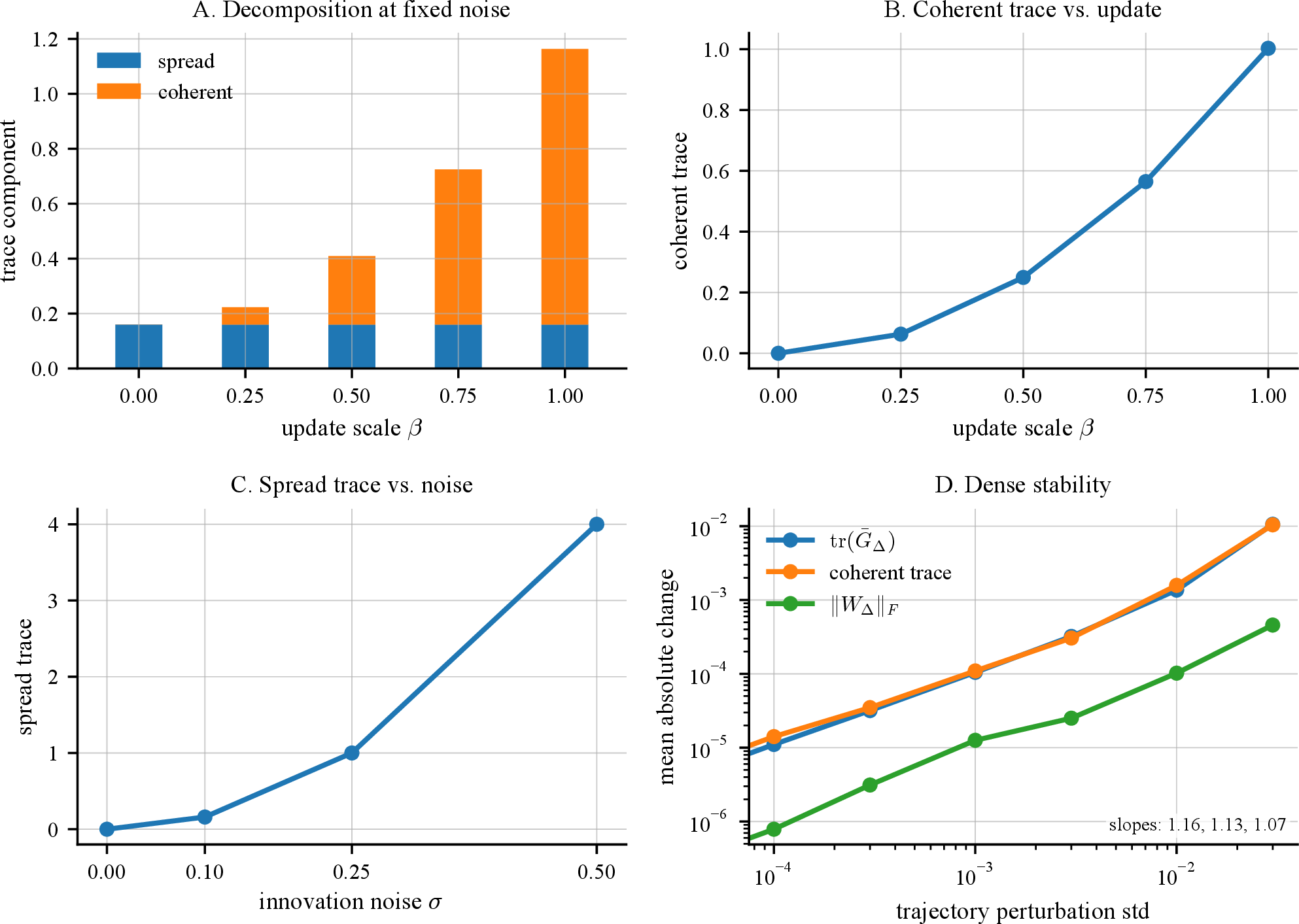
We first validate the linear-Gaussian closed form. We sample \[Y=AX+\xi, \qquad X\sim\mathcal{N}(0,I), \qquad \xi\sim\mathcal{N}(0,\sigma^2I),\] with \(A=I+\beta B\) for fixed Frobenius-normalized \(B\). We sweep \(\beta\in\{0,0.25,0.5,0.75,1.0\}\) and \(\sigma\in\{0,0.1,0.25,0.5\}\) at \(d=16\). Because this experiment tests the population closed form, spread and coherent displacement are computed from the known conditional moments. As predicted, \[\text{coherent trace}=\beta^2, \qquad \text{spread trace}=d\sigma^2.\] Across all settings, the maximum relative error is below \(0.7\%\). A separate two-dimensional sweep with \(A=\alpha I+\gamma J\), where \(J\) is antisymmetric, validates the directed statistic, showing that \(\|\widehat{\mathcal{W}}_\Delta\|_F\) grows approximately linearly with \(\gamma\) and vanishes at \(\gamma=0\), matching the linear-Gaussian formula.
We next test the structural theorems. For affine covariance, we apply translations, orthogonal maps, scalar dilations, and anisotropic diagonal maps to a cyclic-shift trajectory cloud. In the push-forward experiment, the conditional weights are held fixed and the coordinates are transformed. Translations and orthogonal maps preserve Euclidean trace summaries, scalar dilations scale traces by the squared scale, and the metric correction \(M'=A^{-\top}MA^{-1}\) restores the original trace summaries to numerical precision. If the Gaussian kernel is rebuilt after an anisotropic transformation, the estimator itself changes, as expected; this sensitivity is reported separately in Appendix 12.2.
For dense stability, we perturb a fixed cyclic-shift cloud by Gaussian noise of scale \(\sigma_p\), keep the bandwidth fixed, and measure absolute changes in \(\operatorname{tr}(\bar G_\Delta)\), coherent displacement trace, and \(\|\widehat{\mathcal{W}}_\Delta\|_F\), averaged over eight perturbations per scale. The observed slopes are close to one, consistent with Theorem 2. Sparse \(k\)-NN approximations are tested in Appendix [app:knn95sensitivity]. They are useful computationally, but change the local resolution and do not share the dense operator’s Lipschitz guarantee.
5.2 Repeat-copy recurrent case study↩︎
We train Elman, GRU, and LSTM networks on repeat-copy with feature dimension \(4\), using a recall-window-weighted loss. The five-seed performance-matched run uses copy length \(10\); the capacity-control, memory-horizon, and phase-profile experiments use copy length \(8\) in the expanded grids (Appendix 12.4). All main-table runs solve the task: recall sign accuracy is \(1.000\) for Elman and GRU, and \(0.9999\) for LSTM. Table 2 reports dense finite-lag quantities on the hidden state \(h_t\) across five seeds.
| arch | \(\operatorname{tr}(\bar G_\Delta)\) | spread | coherent | \(F_\Delta^\rho\) | static rank |
|---|---|---|---|---|---|
| Elman-64 | \(1.0085\pm0.0008\) | \(1.0018\pm0.0005\) | \(1.0151\pm0.0017\) | \(0.5033\pm0.0005\) | \(25.5\pm0.6\) |
| GRU-64 | \(0.8673\pm0.0076\) | \(0.9294\pm0.0050\) | \(0.8051\pm0.0131\) | \(0.4641\pm0.0039\) | \(12.6\pm1.3\) |
| LSTM-64 | \(0.8815\pm0.0035\) | \(0.8908\pm0.0066\) | \(0.8721\pm0.0132\) | \(0.4947\pm0.0056\) | \(14.0\pm0.7\) |
The strongest architecture-dependent differences are in total transport scale and coherent displacement trace. Elman has larger \(\operatorname{tr}(\bar G_\Delta)\) than GRU and LSTM by roughly \(15\%\), and its coherent trace is larger by \(16\)–\(26\%\). In contrast, the coherent displacement fraction is not a stable architecture identifier: at the median bandwidth it lies near \(0.45\)–\(0.50\), and the sensitivity sweeps below show that it changes with kernel resolution and coordinate normalization.
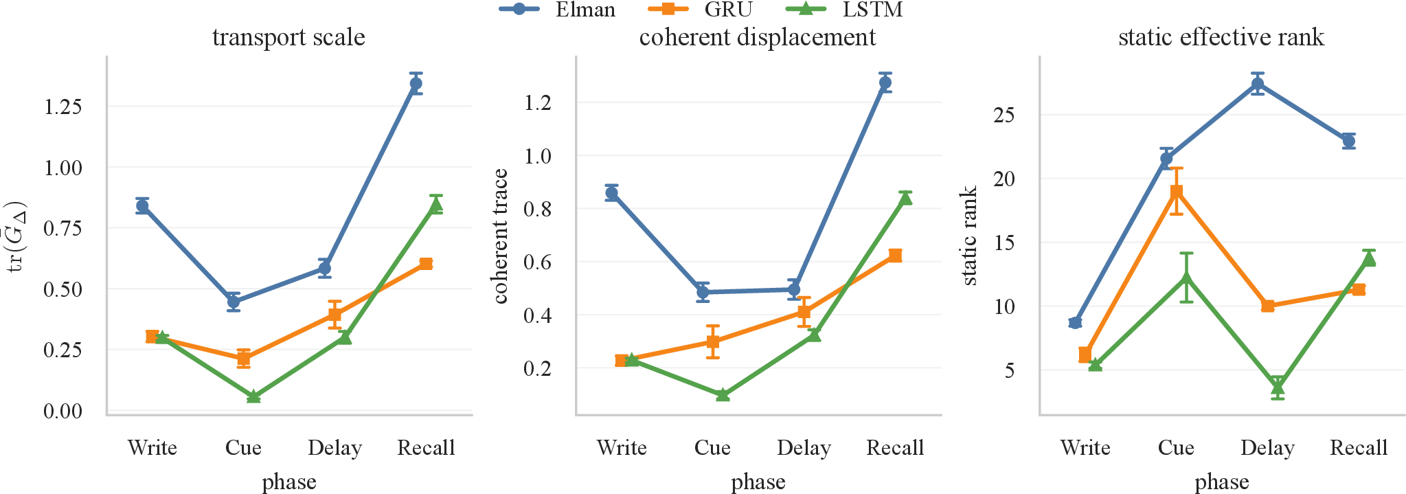
Finally, phase-resolved analysis localizes where the transport differences arise. In a solved repeat-copy setting with delay \(D=4\), we split source–successor pairs into write, cue, delay, and recall phases, apply the same global center-RMS normalization, and compute phase-local dense operators. Figure 2 shows that Elman has substantially larger transport and coherent displacement during write and recall, while GRU and LSTM maintain lower transport through write, cue, and delay and increase at recall. Static effective rank follows a different pattern, showing that finite-lag geometry captures when hidden states move, not only where they sit. Full tables are in Appendix 12.9.
5.2.0.1 Capacity controls and sensitivity.
Parameter-count controls preserve the transport-scale gap. At nearly matched parameter counts, Elman-64 has \(4{,}804\) parameters and \(\operatorname{tr}(\bar G_\Delta)=1.013\pm0.001\), while GRU-36 has \(4{,}792\) parameters and \(\operatorname{tr}(\bar G_\Delta)=0.858\pm0.067\). Across the controlled grid, Elman configurations remain near \(1.01\), while gated configurations lie between \(0.86\) and \(0.89\).
Resolution and metric sweeps explain which scalars are robust. For dense center-RMS operators, narrowing the bandwidth from \(\varepsilon_{\rm med}\) to \(0.1\varepsilon_{\rm med}\) increases coherent displacement fraction from about \(0.50\) to \(0.62\) for Elman, \(0.45\) to \(0.53\) for GRU, and \(0.50\) to \(0.58\) for LSTM. Whitening changes absolute trace scale and shifts the fraction, as predicted by the metric dependence in Theorem 1. Sparse \(k\)-NN approximations produce still more local fractions and larger circulation values. Thus the robust learned-network finding is the transport-scale and coherent-trace separation. Fractions and circulation norms must be read with their metric and resolution choices.
A small-delay memory-horizon sweep gives the same qualitative picture along a task axis. We insert blank delays \(D\in\{0,2,4,6,8\}\) between delimiter and recall. GRU and LSTM solve all delays across three seeds. Elman solves all seeds through \(D=6\) and two of three seeds at \(D=8\). For GRU, \(\operatorname{tr}(\bar G_\Delta)\) decreases from \(0.875\) at \(D=0\) to \(0.716\) at \(D=8\), and coherent trace decreases from \(0.826\) to \(0.563\). LSTM shows the same trend, with transport decreasing from \(0.880\) to \(0.728\) and coherent trace from \(0.842\) to \(0.640\). Circulation increases from near zero to a larger plateau for both gated architectures. Thus the finite-lag observables respond systematically to memory horizon on solved runs. Full tables are in Appendix 12.10.
6 Discussion↩︎
We introduced finite-lag operator geometry as a trajectory-directed counterpart of static diffusion operator geometry. The primitive is a directed empirical transport law on observed source–successor pairs. From this law we derive a source-centered transport tensor \(G_\Delta\), which decomposes exactly into conditional spread and coherent displacement, and an antisymmetric coordinate circulation \(\mathcal{W}_\Delta^\rho\), which summarizes directed finite-lag flow. The framework is built at the lag where the recurrent computation is observed. It does not require estimating an underlying continuous-time generator or assuming that hidden state alone is autonomously Markov.
The structural results clarify what is intrinsic and what is conventional. Affine covariance shows that the tensorial quantities transform naturally, while scalar summaries require a metric choice. Dense stability justifies the smooth Gaussian source-smoothing estimator over hard \(k\)-NN sparsification. Finite-lag separation explains why deterministic recurrent motion can be visible at finite lag even when infinitesimal carré-du-champ geometry is zero. The linear-Gaussian closed form provides an analytical calibration, showing transport scale comes from innovation spread and coherent update displacement, while circulation comes from the antisymmetric mismatch of lagged cross-covariances.
Empirically, controlled systems validate the formal quantities, and a performance-matched repeat-copy case study illustrates their behavior on trained recurrent networks. The most robust finite-lag differences in this case study are total transport scale and coherent displacement trace. In contrast, coherent displacement fraction and circulation norms depend on the chosen metric and kernel resolution, as predicted by the theory. Capacity controls preserve the transport-scale gap, and memory-horizon experiments show that the quantities respond to task demand on solved runs.
These experiments are not intended as universal architecture claims. They demonstrate how finite-lag operator geometry can be used, by calibrating the formal quantities in controlled systems, then report transport scale, conditional spread, coherent displacement, and directed circulation under explicit normalization and bandwidth choices. The broader message is that recurrent representations should be analyzed not only as clouds of states, but as finite-lag transport laws describing where the computation sends those states.
7 Empirical operator construction↩︎
Here we give the operational details of the empirical finite-lag operator \(\widehat P_\Delta\) used throughout the paper. The dense Gaussian source-smoothing estimator of Equation 1 is the object used in the stability theory. The \(k\)-nearest-neighbor version is a scalable approximation and is used only where explicitly stated.
7.1 Lagged-pair pooling and notation↩︎
Hidden trajectories are written \(h_t^{(s)} \in \mathbb{R}^d\), indexed by sequence or trial \(s\) and time \(t\). For a fixed integer lag \(\Delta \ge 1\) and physical lag \(\tau=\Delta\,dt\), define the pooled index set \[\mathcal{X} = \{(s,t): h_t^{(s)} \text{ is observed}\}, \qquad x_p=h_t^{(s)} \quad \text{for } p=(s,t).\] The valid source set is \[\mathcal{X}^- = \{p=(s,t)\in\mathcal{X} : (s,t+\Delta)\in\mathcal{X}\}.\] For \(p\in\mathcal{X}^-\), write \(p+\Delta=(s,t+\Delta)\), define the lagged successor map \(T_\Delta(p)=p+\Delta\), and set \[y_p=x_{T_\Delta(p)}.\] The empirical lagged pair cloud is \[\{(x_p,y_p):p\in\mathcal{X}^-\}.\] We write \(n=|\mathcal{X}^-|\) for the number of valid pairs and \(d\) for the hidden dimension. Unless otherwise stated, the empirical source measure is uniform on \(\mathcal{X}^-\), so \(\rho_p=1/n\).
Throughout the construction, query indices \(q\) and neighbor indices \(i\) range over \(\mathcal{X}^-\). Successor coordinates \(y_i\) may correspond to indices in \(\mathcal{X}\setminus\mathcal{X}^-\), but they are always attached to valid source indices \(i\in\mathcal{X}^-\).
7.2 Dense Gaussian source-smoothing operator↩︎
For bandwidth \(\varepsilon>0\), define the Gaussian source kernel \[K_{qi} = k_\varepsilon(x_q,x_i) = \exp\!\left(-\frac{\|x_q-x_i\|^2}{4\varepsilon}\right), \qquad D_q=\sum_{i\in\mathcal{X}^-}K_{qi}.\] Since \(q\in\mathcal{X}^-\) and \(K_{qq}=1\), each \(D_q\) is strictly positive. The dense empirical source-smoothing operator has normalized weights \[w_{qi} = \frac{K_{qi}}{D_q}, \qquad (\widehat P_\Delta)_{qi}=w_{qi},\] and the corresponding empirical conditional transport law is \[\widehat Q_\Delta(dy\mid x_q) = \sum_{i\in\mathcal{X}^-}w_{qi}\,\delta_{y_i}(dy).\]
The index \(i\) in \((\widehat P_\Delta)_{qi}\) denotes a neighboring source point whose observed successor \(y_i\) contributes to the conditional law at the query source \(x_q\). Thus \(\widehat P_\Delta\) is a source-smoothing operator for a successor-valued empirical law.
We use the Gaussian factor of \(4\) in the bandwidth following the convention used in diffusion-map constructions [9]. This matches the median heuristic bandwidth \[\varepsilon_{\rm med} = \frac{1}{4}\,\operatorname{median}_{i<j}\|x_i-x_j\|^2,\] under which the median pairwise affinity is \(e^{-1}\).
7.3 Empirical observables↩︎
Let \[\bar y_q=\sum_i w_{qi}y_i.\] The empirical squared transport scale, finite-lag drift, source-centered transport tensor, and conditional spread tensor are \[\widehat e_q^{\,2} = \sum_i w_{qi}\|y_i-x_q\|^2, \qquad \widehat m_\Delta(x_q) = \tau^{-1}(\bar y_q-x_q),\] \[\widehat G_\Delta(x_q) = \frac{1}{2\tau} \sum_iw_{qi}(y_i-x_q)(y_i-x_q)^\top,\] and \[\widehat C_\Delta(x_q) = \tau^{-1}\sum_iw_{qi} \bigl[(y_i-x_q)-\tau\widehat m_\Delta(x_q)\bigr] \bigl[(y_i-x_q)-\tau\widehat m_\Delta(x_q)\bigr]^\top.\] Equivalently, since \(\tau\widehat m_\Delta(x_q)=\bar y_q-x_q\), \[\widehat C_\Delta(x_q) = \tau^{-1}\sum_iw_{qi}(y_i-\bar y_q)(y_i-\bar y_q)^\top = \tau^{-1} \left( \sum_iw_{qi}y_i y_i^\top-\bar y_q\bar y_q^\top \right).\] Thus the conditional spread term is the covariance of the smoothed successor cloud attached to the query source.
The pointwise decomposition \[2\,\widehat G_\Delta(x_q) = \widehat C_\Delta(x_q) + \tau\,\widehat m_\Delta(x_q)\widehat m_\Delta(x_q)^\top\] holds exactly by construction. Averaging over a source measure \(\rho\) gives \[\widehat{\bar G}_\Delta^\rho = \sum_q\rho_q\,\widehat G_\Delta(x_q), \qquad \widehat{\bar C}_\Delta^\rho = \sum_q\rho_q\,\widehat C_\Delta(x_q),\] and hence \[2\,\operatorname{tr}(\widehat{\bar G}_\Delta^\rho) = \operatorname{tr}(\widehat{\bar C}_\Delta^\rho) + \tau\sum_q\rho_q\|\widehat m_\Delta(x_q)\|^2.\] We refer to the two terms on the right-hand side as the conditional spread trace and coherent displacement trace, respectively.
For efficient computation, local moments are evaluated chunk-wise to avoid materializing the full \((\text{chunk size},n,d)\) displacement tensor. The squared-distance term is computed using \[\|y_i-x_q\|^2 = \|y_i\|^2+\|x_q\|^2-2y_i^\top x_q.\] For the full transport tensor, we use the identity \[\sum_iw_{qi}(y_i-x_q)(y_i-x_q)^\top = \sum_iw_{qi}y_i y_i^\top - x_q\bar y_q^\top - \bar y_qx_q^\top + x_qx_q^\top.\] The conditional spread tensor is computed using the covariance identity above.
Numerical roundoff in chunk-wise computation can produce a small negative residual in \[\widehat e_q^{\,2}-\tau^2\|\widehat m_\Delta(x_q)\|^2\] at machine precision. We clamp this scalar residual to zero before reporting scalar spread traces, the tensor formulas above are unchanged.
7.4 Empirical coordinate circulation↩︎
The antisymmetric coordinate circulation in the main text is the lagged source–successor cross-moment \[\mathcal{W}_\Delta^\rho = \tau^{-1} \left( \mathbb{E}_\rho[\widetilde{X}\widetilde{Y}^\top] - \mathbb{E}_\rho[\widetilde{Y}\widetilde{X}^\top] \right),\] where \(\widetilde{X},\widetilde{Y}\) denote the chosen normalized coordinates. The default empirical operator estimate uses the same smoothed conditional law \(\widehat Q_\Delta\) as the transport tensor: \[\widehat{\mathcal{W}}_{\Delta,\mathrm{smooth}}^\rho = \tau^{-1} \sum_q\rho_q\sum_iw_{qi} \left( \widetilde{x}_q\widetilde{y}_i^\top - \widetilde{y}_i\widetilde{x}_q^\top \right).\] This matrix is skew-symmetric by construction.
For comparison with population joint-moment calculations, we sometimes also report the raw lagged-pair estimator \[\widehat{\mathcal{W}}_{\Delta,\mathrm{raw}}^\rho = \tau^{-1} \sum_q\rho_q \left( \widetilde{x}_q\widetilde{y}_q^\top - \widetilde{y}_q\widetilde{x}_q^\top \right).\] This is the special case of the smoothed formula obtained by replacing \(w_{qi}\) with \(\mathbf{1}\{i=q\}\). Unless explicitly described as raw, reported circulation values use the smoothed operator estimate.
We summarize circulation by the Frobenius norm \(\|\widehat{\mathcal{W}}_\Delta^\rho\|_F\), the largest imaginary eigenvalue magnitude \(\omega_{\max}\), and the relative circulation \[r_{\rm circ} = \frac{\|\widehat{\mathcal{W}}_\Delta^\rho\|_F}{\operatorname{tr}(\widehat{\bar G}_\Delta^\rho)}.\] The denominator is the total source-centered transport trace in the same coordinate system. When this trace is numerically zero, we leave \(r_{\rm circ}\) undefined rather than reporting an unstable ratio.
7.5 Center-RMS coordinate normalization↩︎
Tensor quantities transform predictably under affine coordinate changes, but Euclidean scalar traces are not invariant under arbitrary linear reparameterizations. Theorem 1 characterizes the exact transformation law for the unnormalized tensorial quantities. In experiments, we adopt center-RMS normalization as a reproducible reporting convention.
Given pooled hidden states \(\{x_p\}_{p\in\mathcal{X}}\), define \[\bar x = |\mathcal{X}|^{-1}\sum_{p\in\mathcal{X}}x_p, \qquad \sigma_{\rm RMS} = \left( |\mathcal{X}|^{-1}\sum_{p\in\mathcal{X}}\|x_p-\bar x\|^2 \right)^{1/2},\] and \[\widetilde{x}_p = \frac{x_p-\bar x}{\sigma_{\rm RMS}}.\] The same affine map is applied to source and successor coordinates: \[\widetilde{y}_p = \frac{y_p-\bar x}{\sigma_{\rm RMS}}.\] Using the same normalization for sources and successors is essential for \(G_\Delta\), \(m_\Delta\), and \(C_\Delta\), since these quantities depend on displacements \(y-x\).
The pooled normalized cloud has empirical mean zero and RMS norm one with respect to the measure used to compute \(\bar x\) and \(\sigma_{\rm RMS}\). When normalization is computed over all pooled hidden states \(\mathcal{X}\), the valid-source subset \(\mathcal{X}^-\) need not have exactly zero mean under \(\rho\). This discrepancy is usually small in the trajectory windows we study, and the same affine coordinate system is applied consistently to sources and successors.
For the circulation statistic, centering affects the decomposition between mean transport and rotational lagged cross-covariance. When the empirical source and successor marginals differ, \(\mathcal{W}_\Delta^\rho\) should be interpreted as an antisymmetric lagged cross-moment in the chosen normalized coordinate system. It may include finite horizon source–successor marginal imbalance in addition to cyclic flow. In stationary or approximately stationary trajectory windows, this coincides with the usual centered lagged cross-covariance interpretation.
Center-RMS normalization preserves Euclidean trace summaries under translations, orthogonal transformations, and global scalar rescalings. It does not preserve them under anisotropic coordinate rescalings. Those require the metric correction of Theorem 1. We use center-RMS normalization in all main-text experiments.
If \(\sigma_{\rm RMS}\) is numerically zero, the trajectory cloud has no nontrivial empirical scale in the chosen window. In that degenerate case the normalized Euclidean summaries are undefined.
7.6 \(k\)-nearest-neighbor approximation↩︎
For larger trajectory clouds, the dense operator becomes computationally expensive. The \(k\)-nearest-neighbor approximation replaces the dense weights with sparse weights restricted to nearby source points.
For a query \(x_q\) and neighborhood size \(k\), let \(\mathcal{N}_k(x_q)\) be the selected source-space neighborhood. We always include \(q\) itself when \(q\in\mathcal{X}^-\), replacing the farthest selected neighbor if necessary. This matches the dense operator’s convention that \(K_{qq}=1\). The remaining non-forced neighbors are chosen by increasing source-space distance, with ties broken by index order. The sparse weights are \[\widetilde{w}_{qi} = \frac{K_{qi}\,\mathbf{1}\{i\in\mathcal{N}_k(x_q)\}}{\sum_{j\in\mathcal{N}_k(x_q)}K_{qj}}.\] The corresponding row-stochastic matrix has at most \(k\) nonzero entries per row.
7.6.0.1 Discontinuity of \(k\)-NN selection.
The \(k\)-NN approximation is not Lipschitz in the source cloud. We record this formally for the non-forced part of the selected neighborhood.
Proposition 2 (Discontinuity of hard \(k\)-NN selection). Consider the \(k\)-nearest-neighbor selection rule on a finite source cloud, excluding any neighbor indices that are fixed by convention, such as a forced self-index. For \(1\le k<|\mathcal{X}|-1\), the selected non-forced neighbor set is discontinuous at any configuration where, for some query \(x_q\), the \(k\)-th and \((k+1)\)-st non-forced neighbor distances are equal. Consequently, any observable that nontrivially depends on the selected adjacency pattern can change by an order-one amount under arbitrarily small perturbations.
Proof. Suppose two candidate non-forced neighbors \(x_p\) and \(x_r\) satisfy \[\|x_q-x_p\|=\|x_q-x_r\|=R,\] with exactly \(k-1\) other non-forced candidates strictly closer to \(x_q\). Suppose the deterministic tie-breaking rule selects \(x_p\) and excludes \(x_r\). For any \(\eta>0\), perturb \(x_r\) by less than \(\eta\) in a direction that makes it strictly closer to \(x_q\), while leaving all other points fixed. The selected neighbor changes from \(x_p\) to \(x_r\), so the corresponding adjacency entry changes by one under an arbitrarily small perturbation. ◻
The dense Gaussian source-smoothing operator does not exhibit this adjacency discontinuity at any fixed bandwidth (Theorem 2). The \(k\)-NN approximation is therefore appropriate for sensitivity studies and large-scale computation, but it introduces an estimator nonsmoothness that the dense operator avoids. The empirical comparison appears in Appendix [app:knn95sensitivity].
7.7 Bandwidth selection↩︎
Unless otherwise stated, we use the median-heuristic bandwidth \[\varepsilon_{\rm med} = \frac{1}{4}\,\operatorname{median}_{i<j}\|x_i-x_j\|^2,\] computed on the source coordinates, with subsampling to at most \(2000\) points when \(n>2000\). The factor of \(4\) matches the kernel denominator. Under this choice the median pairwise affinity is \(e^{-1}\), giving a reproducible default scale for the dense operator.
If the median pairwise squared distance is numerically zero, we replace \(\varepsilon_{\rm med}\) by a small positive floor. Stability statements with adaptive bandwidth should be read on subsets where the selected bandwidth is bounded away from zero. Theorem 2 is stated for fixed \(\varepsilon>0\). When \(\varepsilon\) is selected from the data, the same fixed-bandwidth bound applies conditionally on the selected scale, and additional dependence enters through the bandwidth-selection rule.
We sweep the bandwidth scale \[\varepsilon/\varepsilon_{\rm med} \in \{0.1,0.2,0.3,0.5,1.0,2.0\}\] in the resolution-dependence experiment reported below. Wider bandwidths smooth more aggressively, attribute more trace mass to conditional spread, and increase the effective neighborhood size. Narrower bandwidths resolve more local structure but reduce effective neighborhood size and worsen finite-sample stability constants.
8 Proofs for the framework↩︎
This appendix proves the basic structural propositions used in Section 3. We use the notation of Appendix 7.
8.1 Well-posedness of the empirical operator↩︎
Proposition 3 (Well-posed empirical operator, restated). Suppose \(D_q=\sum_iK_{qi}>0\) at every evaluated source node \(x_q\). Then \(\widehat Q_\Delta(\cdot\mid x_q)\) is a probability measure for every \(q\), \(\widehat P_\Delta\) is a positive operator on bounded observables, and the finite matrix \[(\widehat P_\Delta)_{qi}=w_{qi}\] is row-stochastic.
Proof. The Gaussian kernel is positive, so \(K_{qi}>0\) for all finite source coordinates \(x_q,x_i\). If \(D_q>0\), then \[w_{qi}=\frac{K_{qi}}{D_q}\ge 0, \qquad \sum_i w_{qi}=1.\] Thus \[\widehat Q_\Delta(dy\mid x_q) = \sum_iw_{qi}\delta_{y_i}(dy)\] is a probability measure and the rows of \(\widehat P_\Delta\) sum to one. For any bounded observable \(f\) on hidden-state coordinates, \[(\widehat P_\Delta f)(x_q) = \sum_iw_{qi}f(y_i).\] If \(f\ge 0\), then \(\widehat P_\Delta f\ge 0\), establishing positivity. ◻
In the operating regime of this paper, \(D_q>0\) holds automatically. For \(q\in\mathcal{X}^-\), the self-kernel \(K_{qq}=1\) is included in the sum.
8.2 Coordinate form and positive semidefiniteness↩︎
Motivated by the carré-du-champ covariance formula, define the finite-lag quadratic form on observables \(f,g\) by \[\Gamma_\Delta(f,g)(x) = \frac{1}{2\tau} \int \bigl(f(y)-f(x)\bigr) \bigl(g(y)-g(x)\bigr) \,Q_\Delta(dy\mid x).\]
Proposition 4 (Coordinate form, restated). For coordinate functions \(z_a(u)=u_a\), \[\Gamma_\Delta(z_a,z_b)(x) = \bigl(G_\Delta(x)\bigr)_{ab}.\] Moreover, \(G_\Delta(x)\succeq 0\) for every \(x\).
Proof. Substituting \(z_a(y)-z_a(x)=y_a-x_a\) gives \[\Gamma_\Delta(z_a,z_b)(x) = \frac{1}{2\tau} \int (y_a-x_a)(y_b-x_b)\,Q_\Delta(dy\mid x) = \bigl(G_\Delta(x)\bigr)_{ab}.\] For positive semidefiniteness, let \(v\in\mathbb{R}^d\). Then \[v^\top G_\Delta(x)v = \frac{1}{2\tau} \int \bigl(v^\top(y-x)\bigr)^2 \,Q_\Delta(dy\mid x) \ge 0.\] ◻
For the empirical operator, \[\bigl(\widehat G_\Delta(x_q)\bigr)_{ab} = \frac{1}{2\tau} \sum_iw_{qi} (y_{i,a}-x_{q,a})(y_{i,b}-x_{q,b}),\] and the same quadratic-form argument gives \[\widehat G_\Delta(x_q)\succeq 0\] at every evaluated source node.
8.3 Source-centered decomposition↩︎
Proposition 5 (Source-centered decomposition, restated). Whenever the conditional second moment of \(Y-X\) exists, \[2G_\Delta(x) = C_\Delta(x) + \tau\,m_\Delta(x)m_\Delta(x)^\top.\]
Proof. Condition on \(X=x\) and write \(D=Y-X\). The second-moment identity gives \[\mathbb{E}[DD^\top\mid X=x] = \operatorname{Cov}(D\mid X=x) + \mathbb{E}[D\mid X=x]\mathbb{E}[D\mid X=x]^\top.\] By definition, \[2G_\Delta(x) = \tau^{-1}\mathbb{E}[DD^\top\mid X=x],\] \[C_\Delta(x) = \tau^{-1}\operatorname{Cov}(D\mid X=x), \qquad m_\Delta(x) = \tau^{-1}\mathbb{E}[D\mid X=x].\] Therefore \[2G_\Delta(x) = C_\Delta(x) + \tau^{-1} \mathbb{E}[D\mid X=x]\mathbb{E}[D\mid X=x]^\top.\] Since \(\mathbb{E}[D\mid X=x]=\tau m_\Delta(x)\), the second term is \[\tau\,m_\Delta(x)m_\Delta(x)^\top.\] ◻
The empirical identity \[2\widehat G_\Delta(x_q) = \widehat C_\Delta(x_q) + \tau\,\widehat m_\Delta(x_q)\widehat m_\Delta(x_q)^\top\] holds pointwise by the same argument with finite sums. Taking traces and averaging against \(\rho\) gives Equation 2 .
8.4 Deterministic transport corollary↩︎
Corollary 1 (Deterministic transport). If \(Y=T_\Delta(x)\) deterministically given \(X=x\), then \[G_\Delta(x) = \frac{1}{2\tau} \bigl(T_\Delta(x)-x\bigr) \bigl(T_\Delta(x)-x\bigr)^\top.\] In particular, \(G_\Delta(x)\ne 0\) whenever \(T_\Delta(x)\ne x\).
Proof. Under deterministic transport, \[\operatorname{Cov}(Y-X\mid X=x)=0, \qquad \mathbb{E}[Y-X\mid X=x]=T_\Delta(x)-x.\] Substituting into Definition 2 gives the stated formula. The rank-one matrix is zero if and only if \(T_\Delta(x)=x\). ◻
This is a population statement for the exact conditional law. At finite bandwidth, the dense empirical estimator can have nonzero \(\widehat C_\Delta(x_q)\) even for deterministic underlying dynamics, because \(\widehat Q_\Delta(\cdot\mid x_q)\) averages successors attached to nearby source points. This is the finite-resolution spread of the empirical operator.
8.5 Abstract finite-state current and detailed balance↩︎
This subsection records standard current identities for a row-stochastic Markov matrix on a common finite state space. These identities apply directly when \(P_\Delta\) is interpreted as a transition matrix whose row and column indices refer to the same state nodes. For the empirical source-smoothing matrix \(\widehat P_\Delta\), the same algebra defines a source-neighborhood imbalance diagnostic.
Proposition 6 (Skew-symmetry of \(J^\rho\)). Let \(P_\Delta\) be a row-stochastic matrix on a common finite state space. For any distribution \(\rho\) on that state space, define \[J^\rho_{pq} = \rho_p(P_\Delta)_{pq} - \rho_q(P_\Delta)_{qp}.\] Then \[(J^\rho)^\top=-J^\rho.\]
Proof. By definition, \[J^\rho_{qp} = \rho_q(P_\Delta)_{qp} - \rho_p(P_\Delta)_{pq} = -J^\rho_{pq}.\] ◻
Proposition 7 (Detailed balance characterization). Let \(P_\Delta\) be a row-stochastic matrix on a common finite state space, and let \(\pi\) be stationary: \[\pi^\top P_\Delta=\pi^\top.\] Then \(J^\pi=0\) if and only if \(P_\Delta\) satisfies detailed balance with respect to \(\pi\): \[\pi_p(P_\Delta)_{pq} = \pi_q(P_\Delta)_{qp} \qquad \text{for all }p,q.\]
Proof. The condition \(J^\pi_{pq}=0\) for all \(p,q\) is exactly \[\pi_p(P_\Delta)_{pq} = \pi_q(P_\Delta)_{qp} \qquad \text{for all }p,q,\] which is detailed balance. ◻
8.5.0.1 Current divergence.
For any distribution \(\rho\), define \[\operatorname{div}_\rho(p) = \sum_q J^\rho_{pq}.\] Using row-stochasticity, \[\operatorname{div}_\rho(p) = \sum_q \left[ \rho_p(P_\Delta)_{pq} - \rho_q(P_\Delta)_{qp} \right] = \rho_p - (\rho^\top P_\Delta)_p.\] If \(\rho=\pi\) is stationary, then \[\operatorname{div}_\rho(p)=0 \qquad \text{for all }p.\] For nonstationary \(\rho\), this divergence is the nodewise imbalance between \(\rho\) and its one-step pushforward \(\rho^\top P_\Delta\).
8.6 Skew-symmetry of coordinate circulation↩︎
Proposition 8 (Skew-symmetry of \(\mathcal{W}_\Delta^\rho\)). The coordinate circulation \[\mathcal{W}_\Delta^\rho = \tau^{-1} \left( \mathbb{E}_\rho[\widetilde{X}\,\widetilde{Y}^\top] - \mathbb{E}_\rho[\widetilde{Y}\,\widetilde{X}^\top] \right)\] is real and skew-symmetric for any source measure \(\rho\). Hence its eigenvalues are purely imaginary and occur in conjugate pairs. If \(Q_\Delta\) is a Markov transition law on a common state space with stationary distribution \(\pi\), and if detailed balance holds with respect to \(\pi\), then \[\mathcal{W}_\Delta^\pi=0.\]
Proof. Taking the transpose gives \[(\mathcal{W}_\Delta^\rho)^\top = \tau^{-1} \left( \mathbb{E}_\rho[\widetilde{Y}\,\widetilde{X}^\top] - \mathbb{E}_\rho[\widetilde{X}\,\widetilde{Y}^\top] \right) = -\mathcal{W}_\Delta^\rho.\] Thus \(\mathcal{W}_\Delta^\rho\) is real and skew-symmetric. A real skew-symmetric matrix is normal and has purely imaginary eigenvalues, occurring in conjugate pairs.
For the reversible case, detailed balance gives exchangeability of the stationary two-time law: \[\pi(dx)Q_\Delta(dy\mid x) = \pi(dy)Q_\Delta(dx\mid y).\] Therefore \[\mathbb{E}_\pi[\widetilde{X}\,\widetilde{Y}^\top] = \mathbb{E}_\pi[\widetilde{Y}\,\widetilde{X}^\top],\] and hence \[\mathcal{W}_\Delta^\pi=0.\] ◻
The Frobenius norm \[\|\mathcal{W}_\Delta^\rho\|_F,\] the maximum imaginary eigenvalue magnitude \[\omega_{\max} = \max_\lambda |\operatorname{Im}\lambda(\mathcal{W}_\Delta^\rho)|,\] and the relative circulation \[r_{\rm circ} = \frac{\|\mathcal{W}_\Delta^\rho\|_F}{\operatorname{tr}(\bar G_\Delta^\rho)}\] are invariant under orthogonal coordinate changes. Under the center-RMS normalization convention of Appendix 7.5, the relative circulation is also invariant to global scalar rescaling whenever the denominator is nonzero.
8.7 Source current and coordinate circulation↩︎
The source current \(J^\rho\) and the coordinate circulation \(\mathcal{W}_\Delta^\rho\) are distinct finite-lag diagnostics.
The current \(J^\rho\) is a node-level object for a finite-state Markov matrix. It records pairwise imbalance \[\rho_p(P_\Delta)_{pq}-\rho_q(P_\Delta)_{qp}\] and gives the detailed-balance characterization above. When applied to the empirical source-smoothing matrix, it measures imbalance between source neighborhood weights.
The coordinate circulation \(\mathcal{W}_\Delta^\rho\) is a coordinate-level antisymmetric moment between sources and successors. It is the object used for representation-geometric reporting. In the linear-Gaussian model of Theorem 4, it has the closed form \[\mathcal{W}_\Delta = \tau^{-1} \left( \Sigma A_\Delta^\top - A_\Delta\Sigma \right).\]
For Markov chains on a unified finite state space, coordinate-level circulations can be obtained by contracting node currents with coordinate observables. In the empirical source–successor construction used here, source indices and successor observations are paired but are not identified as the same finite state nodes by the source smoother. We therefore keep \(J^\rho\) as a finite-state imbalance object and \(\mathcal{W}_\Delta^\rho\) as the coordinate-level circulation statistic.
9 Proofs of Structural Properties of Finite-Lag Geometry↩︎
This appendix proves the structural theorems of Section 4. Notation follows Appendix 7. We write \[\mathcal{Z}=\{(x_i,y_i)\}_{i=1}^n\] for a paired source–successor cloud and \[\|\mathcal{Z}-\widetilde{\mathcal{Z}}\|_\infty = \max_i\max\{\|x_i-\widetilde{x}_i\|,\|y_i-\widetilde{y}_i\|\}\] for the perturbation size.
9.1 Affine covariance↩︎
Theorem 5 (Affine covariance and metric dependence, restated). Let \(\phi(x)=Ax+b\), with \(A\in\mathbb{R}^{d\times d}\) invertible, and let \(Q'_\Delta\) be the pushed-forward conditional law \[Q'_\Delta(B\mid x') = Q_\Delta(\phi^{-1}(B)\mid \phi^{-1}(x')).\] Let \(\rho'=\phi_\#\rho\) be the pushed-forward source measure. The following covariance statements are for the unnormalized tensorial quantities. For \(\mathcal{W}_\Delta^\rho\), centered coordinates are used before any RMS renormalization.
Then, for \(x'=\phi(x)\), \[m'_\Delta(x')=A\,m_\Delta(x), \qquad C'_\Delta(x')=A\,C_\Delta(x)\,A^\top,\] \[G'_\Delta(x')=A\,G_\Delta(x)\,A^\top, \qquad (\mathcal{W}'_\Delta)^{\rho'} = A\,\mathcal{W}_\Delta^\rho\,A^\top.\] The decomposition identity is coordinate-covariant: \[2G'_\Delta(x') = C'_\Delta(x') + \tau\,m'_\Delta(x')m'_\Delta(x')^\top.\]
For \(M\succ0\), define the metric-weighted spread and coherent displacement summaries by \[S_C^M = \int \operatorname{tr}\!\bigl(MC_\Delta(x)\bigr)\,\rho(dx), \qquad S_m^M = \tau\int m_\Delta(x)^\top M m_\Delta(x)\,\rho(dx),\] and \[F^M = \frac{S_m^M}{S_C^M+S_m^M}\] whenever the denominator is nonzero. Under the metric transformation \[M'=A^{-\top}MA^{-1},\] one has \[S_{C'}^{M'}=S_C^M, \qquad S_{m'}^{M'}=S_m^M, \qquad F^{M'}=F^M.\]
Proof. Let \(D=Y-X\). Under the affine change of coordinates, \[D'=Y'-X'=A(Y-X)=AD.\] Therefore \[\mathbb{E}[D'\mid X'=x'] = A\,\mathbb{E}[D\mid X=x],\] and \[\operatorname{Cov}(D'\mid X'=x') = A\,\operatorname{Cov}(D\mid X=x)\,A^\top.\] Dividing by \(\tau\) gives \[m'_\Delta(x')=A\,m_\Delta(x), \qquad C'_\Delta(x')=A\,C_\Delta(x)\,A^\top.\] Similarly, \[G'_\Delta(x') = \frac{1}{2\tau} \mathbb{E}[D'D'^\top\mid X'=x'] = \frac{1}{2\tau} A\,\mathbb{E}[DD^\top\mid X=x]\,A^\top = A\,G_\Delta(x)\,A^\top.\] Substituting these identities into the source-centered decomposition gives \[2G'_\Delta(x') = C'_\Delta(x') + \tau\,m'_\Delta(x')m'_\Delta(x')^\top.\]
For circulation, let \(\widetilde{X},\widetilde{Y}\) denote centered coordinates in the original system and \(\widetilde{X}',\widetilde{Y}'\) centered coordinates in the transformed system, before RMS renormalization. Centering removes the translation \(b\), so \[\widetilde{X}'=A\widetilde{X}, \qquad \widetilde{Y}'=A\widetilde{Y}.\] Thus \[(\mathcal{W}'_\Delta)^{\rho'} = \tau^{-1} \left( \mathbb{E}_{\rho'}[\widetilde{X}'\widetilde{Y}'^\top] - \mathbb{E}_{\rho'}[\widetilde{Y}'\widetilde{X}'^\top] \right)\] \[= \tau^{-1} \left( A\,\mathbb{E}_\rho[\widetilde{X}\widetilde{Y}^\top]\,A^\top - A\,\mathbb{E}_\rho[\widetilde{Y}\widetilde{X}^\top]\,A^\top \right) = A\,\mathcal{W}_\Delta^\rho\,A^\top.\]
For the metric-weighted summaries, cyclicity of trace gives \[\operatorname{tr}\!\bigl(M'C'_\Delta(x')\bigr) = \operatorname{tr}\!\bigl( A^{-\top}MA^{-1}AC_\Delta(x)A^\top \bigr) = \operatorname{tr}\!\bigl(MC_\Delta(x)\bigr).\] Likewise, \[m'_\Delta(x')^\top M'm'_\Delta(x') = (Am_\Delta(x))^\top A^{-\top}MA^{-1}(Am_\Delta(x)) = m_\Delta(x)^\top M m_\Delta(x).\] Integrating against the pushed-forward source measure gives \[S_{C'}^{M'}=S_C^M, \qquad S_{m'}^{M'}=S_m^M.\] The fraction \(F^M=S_m^M/(S_C^M+S_m^M)\) is invariant because both numerator and denominator are invariant. ◻
The Euclidean trace convention \(M=I\) is invariant under translations and orthogonal transformations. Under global scalar rescaling, center-RMS normalization removes the scalar factor before Euclidean traces are reported. Anisotropic reparameterizations require the metric correction above.
9.2 Stability of the dense empirical operator↩︎
The proof of Theorem 2 uses three elementary bounds, one for squared distances, one for Gaussian kernel entries, and one for row-normalization.
Lemma 1 (Squared-distance perturbation). Let \(\mathcal{Z},\widetilde{\mathcal{Z}}\) satisfy \[\max_i \{ \|x_i\|,\|y_i\|,\|\widetilde{x}_i\|,\|\widetilde{y}_i\| \} \le R.\] Then, for all \(i,j\), \[\left| \|x_i-x_j\|^2-\|\widetilde{x}_i-\widetilde{x}_j\|^2 \right| \le 8R\,\|\mathcal{Z}-\widetilde{\mathcal{Z}}\|_\infty.\] The same bound holds for squared distances formed from any corresponding source or successor coordinates.
Proof. Let \[a=x_i-x_j, \qquad b=\widetilde{x}_i-\widetilde{x}_j.\] Then \[\|a\|^2-\|b\|^2 = \langle a+b,a-b\rangle,\] so \[\left|\|a\|^2-\|b\|^2\right| \le \|a+b\|\,\|a-b\|.\] The boundedness assumption gives \[\|a\|\le2R, \qquad \|b\|\le2R, \qquad \|a+b\|\le4R.\] Also, \[\|a-b\| = \|(x_i-\widetilde{x}_i)-(x_j-\widetilde{x}_j)\| \le 2\|\mathcal{Z}-\widetilde{\mathcal{Z}}\|_\infty.\] Multiplying the two bounds gives the claim. ◻
Lemma 2 (Kernel perturbation). For the Gaussian kernel \[K_{qi}=k_\varepsilon(x_q,x_i) = \exp\!\left(-\frac{\|x_q-x_i\|^2}{4\varepsilon}\right),\] one has \[|K_{qi}(\mathcal{Z})-K_{qi}(\widetilde{\mathcal{Z}})| \le \frac{2R}{\varepsilon}\, \|\mathcal{Z}-\widetilde{\mathcal{Z}}\|_\infty.\]
Proof. The function \[u\mapsto e^{-u/(4\varepsilon)}\] has derivative \[-\frac{1}{4\varepsilon}e^{-u/(4\varepsilon)},\] whose absolute value is at most \(1/(4\varepsilon)\) for \(u\ge0\). By Lemma 1, \[|K_{qi}(\mathcal{Z})-K_{qi}(\widetilde{\mathcal{Z}})| \le \frac{1}{4\varepsilon} \left| \|x_q-x_i\|^2-\|\widetilde{x}_q-\widetilde{x}_i\|^2 \right| \le \frac{2R}{\varepsilon} \|\mathcal{Z}-\widetilde{\mathcal{Z}}\|_\infty.\] ◻
Lemma 3 (Row-normalization Lipschitz bound). Let \(W,\widetilde{W}\in\mathbb{R}_{\ge0}^{n\times n}\) have row sums \[D_q=\sum_jW_{qj}\ge n\beta, \qquad \widetilde{D}_q=\sum_j\widetilde{W}_{qj}\ge n\beta\] for some \(\beta>0\). Let \[w_{qi}=\frac{W_{qi}}{D_q}, \qquad \widetilde{w}_{qi}=\frac{\widetilde{W}_{qi}}{\widetilde{D}_q}.\] If \[\max_{q,i}|W_{qi}-\widetilde{W}_{qi}|\le\delta,\] then, for every \(q\), \[\sum_i|w_{qi}-\widetilde{w}_{qi}| \le \frac{2\delta}{\beta}.\]
Proof. Fix \(q\) and write \[W_i=W_{qi}, \qquad \widetilde{W}_i=\widetilde{W}_{qi}, \qquad D=D_q, \qquad \widetilde{D}=\widetilde{D}_q.\] Then \[\sum_i|W_i-\widetilde{W}_i|\le n\delta, \qquad |D-\widetilde{D}|\le n\delta.\] For each \(i\), \[\left| \frac{W_i}{D} - \frac{\widetilde{W}_i}{\widetilde{D}} \right| \le \frac{|W_i-\widetilde{W}_i|}{D} + \widetilde{W}_i \left| \frac{1}{D}-\frac{1}{\widetilde{D}} \right|\] \[= \frac{|W_i-\widetilde{W}_i|}{D} + \widetilde{W}_i \frac{|D-\widetilde{D}|}{D\widetilde{D}}.\] Summing over \(i\) gives \[\sum_i|w_{qi}-\widetilde{w}_{qi}| \le \frac{n\delta}{D} + \frac{|D-\widetilde{D}|}{D\widetilde{D}} \sum_i\widetilde{W}_i.\] Since \(\sum_i\widetilde{W}_i=\widetilde{D}\), \[\sum_i|w_{qi}-\widetilde{w}_{qi}| \le \frac{n\delta}{D} + \frac{|D-\widetilde{D}|}{D} \le \frac{2n\delta}{D}.\] Using \(D\ge n\beta\) yields \[\sum_i|w_{qi}-\widetilde{w}_{qi}| \le \frac{2\delta}{\beta}.\] ◻
Theorem 6 (Dense stability, restated). Fix bandwidth \(\varepsilon>0\) and radius \(R>0\). On the set of paired clouds satisfying \[\max_i\{\|x_i\|,\|y_i\|\}\le R,\] the dense source-smoothing operator satisfies \[\left\| \widehat P_\Delta(\mathcal{Z}) - \widehat P_\Delta(\widetilde{\mathcal{Z}}) \right\|_{\infty\to\infty} \le \frac{4R}{\varepsilon} \exp\!\left(\frac{R^2}{\varepsilon}\right) \|\mathcal{Z}-\widetilde{\mathcal{Z}}\|_\infty\] whenever both clouds lie in this bounded set.
Proof. By Lemma 2, \[|K_{qi}(\mathcal{Z})-K_{qi}(\widetilde{\mathcal{Z}})| \le \delta := \frac{2R}{\varepsilon} \|\mathcal{Z}-\widetilde{\mathcal{Z}}\|_\infty.\] On the radius-\(R\) set, \[\|x_q-x_i\|\le2R,\] so each Gaussian kernel entry is bounded below by \[K_{qi}(\mathcal{Z}) \ge \exp\!\left(-\frac{(2R)^2}{4\varepsilon}\right) = \exp\!\left(-\frac{R^2}{\varepsilon}\right) =:\beta.\] The same lower bound holds for \(\widetilde{K}_{qi}\). Thus every row sum is at least \(n\beta\). Applying Lemma 3 gives, for each row \(q\), \[\sum_i |w_{qi}(\mathcal{Z})-w_{qi}(\widetilde{\mathcal{Z}})| \le \frac{2\delta}{\beta} = \frac{4R}{\varepsilon} \exp\!\left(\frac{R^2}{\varepsilon}\right) \|\mathcal{Z}-\widetilde{\mathcal{Z}}\|_\infty.\] Taking the maximum row sum gives the \(\infty\to\infty\) operator norm bound. ◻
9.2.0.1 Stability of derived observables.
The empirical observables \[\widehat m_\Delta,\quad \widehat G_\Delta,\quad \widehat C_\Delta,\quad \widehat{\mathcal{W}}_\Delta^\rho,\] and their scalar trace summaries inherit Lipschitz dependence on \(\mathcal{Z}\) on bounded sets.
For example, \[\widehat m_\Delta(x_q) = \tau^{-1}\left[ (\widehat P_\Delta Y)_q-x_q \right],\] where \(Y\) is the matrix of successor coordinates. The term \((\widehat P_\Delta Y)_q\) is Lipschitz because both \(\widehat P_\Delta\) and \(Y\) are Lipschitz in the paired cloud on the bounded set, and the term \(-x_q\) is directly Lipschitz.
Similarly, \[\widehat G_\Delta(x_q) = \frac{1}{2\tau} \sum_iw_{qi}(y_i-x_q)(y_i-x_q)^\top.\] Each entry is a row-weighted sum of bounded quadratic functions of the coordinates. Perturbations enter through the weights and through the coordinate factors, both linearly in \(\|\mathcal{Z}-\widetilde{\mathcal{Z}}\|_\infty\) on bounded sets. The same argument applies to \(\widehat C_\Delta\), using either its covariance form or the decomposition \[\widehat C_\Delta = 2\widehat G_\Delta - \tau\,\widehat m_\Delta\widehat m_\Delta^\top.\] The smoothed empirical circulation \[\widehat{\mathcal{W}}_\Delta^\rho = \tau^{-1} \sum_q\rho_q\sum_iw_{qi} \left( \widetilde{x}_q\widetilde{y}_i^\top - \widetilde{y}_i\widetilde{x}_q^\top \right)\] is a weighted bilinear coordinate moment and is Lipschitz by the same bounded-product argument.
Thus the derived observables are Lipschitz on bounded sets at fixed \(\varepsilon>0\). Their constants are polynomial in \(R\) and \(\tau^{-1}\), with the dense-operator dependence entering through the factor \[\frac{1}{\varepsilon} \exp\!\left(\frac{R^2}{\varepsilon}\right).\]
9.2.0.2 Stability after center-RMS normalization.
The main experiments compute observables after center-RMS normalization (Appendix 7.5). The center-RMS map is smooth away from collapsed clouds and ill-conditioned near \(\sigma_{\rm RMS}=0\). Hence the same stability conclusions extend to normalized observables on subsets where \[\sigma_{\rm RMS}\ge\sigma_0>0.\] On such subsets, the resulting constants are polynomial in \(R\), \(1/\sigma_0\), and \(\tau^{-1}\), together with the fixed-bandwidth dense-operator constant above. Near collapsed clouds, where \(\sigma_{\rm RMS}\to0\), the normalization itself is ill-conditioned.
9.3 Finite-lag separation↩︎
Theorem 7 (Finite-lag detection of deterministic motion, restated). Let \(T:\mathbb{R}^d\to\mathbb{R}^d\) be measurable and fix \(\Delta\ge1\). Assume \[\int \|T^\Delta(x)-x\|^2\,\rho(dx)<\infty\] and suppose \(T^\Delta(x)\ne x\) on a \(\rho\)-positive set. If \[X_{t+\Delta}=T^\Delta(X_t)\] deterministically, then \[\bar G_\Delta^\rho = \frac{1}{2\tau} \int \bigl(T^\Delta(x)-x\bigr) \bigl(T^\Delta(x)-x\bigr)^\top \,\rho(dx),\] and \[\operatorname{tr}(\bar G_\Delta^\rho)>0\] at the chosen lag \(\tau\).
For an oriented cyclic shift \(T^\Delta=\Pi\) in centered coordinates with \[\operatorname{Cov}(X)=\sigma_x^2I,\] one has \[\|\mathcal{W}_\Delta^\rho\|_F = \frac{\sigma_x^2}{\tau} \|\Pi^\top-\Pi\|_F > 0\] whenever \(\Pi\) is not symmetric.
By contrast, if a deterministic continuous-time flow \[\dot{X}_t=b(X_t)\] is represented by the first-order generator \(L=b\cdot\nabla\), then its infinitesimal carré du champ satisfies \[\Gamma_L\equiv0.\]
Proof. Under deterministic dynamics, Corollary 1 gives \[G_\Delta(x) = \frac{1}{2\tau} \bigl(T^\Delta(x)-x\bigr) \bigl(T^\Delta(x)-x\bigr)^\top.\] Averaging against \(\rho\) gives the displayed formula for \(\bar G_\Delta^\rho\). Taking traces gives \[\operatorname{tr}(\bar G_\Delta^\rho) = \frac{1}{2\tau} \int \|T^\Delta(x)-x\|^2 \,\rho(dx).\] The integrand is nonnegative and strictly positive on a \(\rho\)-positive set, so the integral is strictly positive.
For the cyclic shift, let \(Y=\Pi X\). In centered coordinates with \(\mathbb{E}[XX^\top]=\sigma_x^2I\), \[\mathbb{E}[XY^\top] = \mathbb{E}[XX^\top\Pi^\top] = \sigma_x^2\Pi^\top,\] and \[\mathbb{E}[YX^\top] = \Pi\mathbb{E}[XX^\top] = \sigma_x^2\Pi.\] Therefore \[\mathcal{W}_\Delta^\rho = \tau^{-1} \left( \sigma_x^2\Pi^\top-\sigma_x^2\Pi \right) = \frac{\sigma_x^2}{\tau} (\Pi^\top-\Pi),\] so \[\|\mathcal{W}_\Delta^\rho\|_F = \frac{\sigma_x^2}{\tau} \|\Pi^\top-\Pi\|_F.\] This is positive whenever \(\Pi^\top\ne\Pi\).
For the infinitesimal contrast, let \(L=b\cdot\nabla\). Since \(L\) is first order, it satisfies the Leibniz rule: \[L(fg)=fLg+gLf.\] Thus \[\Gamma_L(f,g) = \frac{1}{2} \left( L(fg)-fLg-gLf \right) = 0\] for all smooth \(f,g\). Hence \(\Gamma_L\equiv0\). ◻
9.4 Linear-Gaussian closed form↩︎
Theorem 8 (Linear-Gaussian closed form, restated). Let \[X_{t+\Delta}=A_\Delta X_t+\xi_t,\] where \(X_t\) has mean zero and covariance \(\Sigma\), and where \(\xi_t\) is independent of \(X_t\), mean zero, with covariance \(\Sigma_\xi\). Then \[m_\Delta(x) = \tau^{-1}(A_\Delta-I)x, \qquad C_\Delta(x) = \tau^{-1}\Sigma_\xi,\] \[\bar G_\Delta = \frac{1}{2\tau} \left[ \Sigma_\xi + (A_\Delta-I)\Sigma(A_\Delta-I)^\top \right],\] and \[\mathcal{W}_\Delta = \tau^{-1} \left( \Sigma A_\Delta^\top - A_\Delta\Sigma \right).\]
Proof. Given \(X_t=x\), the finite-lag displacement is \[D = X_{t+\Delta}-X_t = (A_\Delta-I)x+\xi_t.\] Since \(\xi_t\) is independent of \(X_t\) and has mean zero, \[\mathbb{E}[D\mid X_t=x] = (A_\Delta-I)x,\] and \[\operatorname{Cov}(D\mid X_t=x) = \Sigma_\xi.\] Dividing by \(\tau\) gives \[m_\Delta(x) = \tau^{-1}(A_\Delta-I)x, \qquad C_\Delta(x) = \tau^{-1}\Sigma_\xi.\] Using the source-centered decomposition, \[2G_\Delta(x) = \tau^{-1}\Sigma_\xi + \tau^{-1} (A_\Delta-I)xx^\top(A_\Delta-I)^\top.\] Averaging over \(X_t\), with \[\mathbb{E}[X_tX_t^\top]=\Sigma,\] gives \[\bar G_\Delta = \frac{1}{2\tau} \left[ \Sigma_\xi + (A_\Delta-I)\Sigma(A_\Delta-I)^\top \right].\]
For circulation, \[\mathbb{E}[X_tX_{t+\Delta}^\top] = \mathbb{E}\!\left[ X_t(A_\Delta X_t+\xi_t)^\top \right] = \Sigma A_\Delta^\top,\] because \(\mathbb{E}[X_t\xi_t^\top]=0\). Similarly, \[\mathbb{E}[X_{t+\Delta}X_t^\top] = \mathbb{E}\!\left[ (A_\Delta X_t+\xi_t)X_t^\top \right] = A_\Delta\Sigma.\] Therefore \[\mathcal{W}_\Delta = \tau^{-1} \left( \Sigma A_\Delta^\top - A_\Delta\Sigma \right).\] ◻
The trace decomposition becomes \[2\,\operatorname{tr}(\bar G_\Delta) = \tau^{-1}\operatorname{tr}(\Sigma_\xi) + \tau^{-1} \operatorname{tr} \left( (A_\Delta-I)\Sigma(A_\Delta-I)^\top \right).\] Thus the conditional spread trace is \[\tau^{-1}\operatorname{tr}(\Sigma_\xi),\] and the coherent displacement trace is \[\tau^{-1} \operatorname{tr} \left( (A_\Delta-I)\Sigma(A_\Delta-I)^\top \right).\] These formulas are stated in centered coordinates before empirical normalization. After applying center-RMS normalization, the same identities hold for the normalized variables and their transformed covariance matrices. They give the parametric calibration used in Section 4.4 and the mechanism signatures in Appendix 10.
10 Linear-Gaussian mechanism signatures↩︎
This appendix specializes the linear-Gaussian closed form (Theorem 8) to several canonical recurrent mechanisms. These examples are analytical calibrations, showing how the framework’s observables respond to simple update structures, and providing reference patterns for interpreting trained-network measurements. We then make explicit the structural parallel between this recurrent closed form and the Gaussian bridge in static feedforward operator geometry.
10.1 Zero-circulation relaxation and isotropic contraction↩︎
Suppose \[A_\Delta \Sigma = \Sigma A_\Delta^\top .\] Then by Theorem 8, \[\mathcal{W}_\Delta = \tau^{-1} \left( \Sigma A_\Delta^\top - A_\Delta \Sigma \right) = 0.\] Thus a linear-Gaussian system can have large finite-lag transport scale while having no antisymmetric coordinate circulation. The condition above is the zero-circulation condition for the lagged cross-moment.
For isotropic contraction, \[A_\Delta=\alpha I, \qquad \alpha\in\mathbb{R},\] we obtain \[\bar G_\Delta = \frac{1}{2\tau} \left[ \Sigma_\xi + (\alpha-1)^2\Sigma \right], \qquad \mathcal{W}_\Delta=0.\] The conditional spread trace is \[\tau^{-1}\operatorname{tr}(\Sigma_\xi),\] and the coherent displacement trace is \[\tau^{-1} (\alpha-1)^2\operatorname{tr}(\Sigma).\] Hence the coherent displacement fraction is \[F_\Delta = \frac{ (\alpha-1)^2\operatorname{tr}(\Sigma) }{ \operatorname{tr}(\Sigma_\xi) + (\alpha-1)^2\operatorname{tr}(\Sigma) }.\] At fixed innovation covariance, \(F_\Delta=0\) when \(\alpha=1\), and \(F_\Delta\to1\) as \(|\alpha-1|\to\infty\). Isotropic contraction therefore increases coherent transport scale without creating coordinate circulation.
10.2 Two-dimensional rotation↩︎
Let \(d=2\), let \[\Sigma=\sigma_x^2 I,\] and let \[A_\Delta=rR_\theta, \qquad R_\theta = \begin{pmatrix} \cos\theta & -\sin\theta \\ \sin\theta & \cos\theta \end{pmatrix}.\] Then \[\Sigma A_\Delta^\top - A_\Delta\Sigma = r\sigma_x^2 \left( R_\theta^\top-R_\theta \right).\] Since \[R_\theta^\top-R_\theta = 2\sin\theta \begin{pmatrix} 0 & 1 \\ -1 & 0 \end{pmatrix},\] the circulation matrix is \[\mathcal{W}_\Delta = \frac{2r\sigma_x^2\sin\theta}{\tau} \begin{pmatrix} 0 & 1 \\ -1 & 0 \end{pmatrix}.\] Its Frobenius norm is \[\|\mathcal{W}_\Delta\|_F = \frac{2\sqrt 2\,r\sigma_x^2|\sin\theta|}{\tau}.\] Thus the antisymmetric statistic grows linearly with radial gain \(r\), source variance \(\sigma_x^2\), and oriented angle magnitude \(|\sin\theta|\), and vanishes exactly when \(\sin\theta=0\).
For pure rotation, \(r=1\) and \(\Sigma_\xi=0\). In that case, \[\bar G_\Delta = \frac{1}{2\tau} (R_\theta-I)\Sigma(R_\theta-I)^\top.\] Using \[(R_\theta-I)(R_\theta-I)^\top = 2(1-\cos\theta)I,\] we get \[\bar G_\Delta = \frac{\sigma_x^2(1-\cos\theta)}{\tau}I.\] Pure rotation therefore produces symmetric transport scale through \(1-\cos\theta\) and antisymmetric circulation through \(\sin\theta\). The two components distinguish displacement magnitude from oriented finite-lag flow.
10.3 Permutation and shift transport↩︎
Let \(A_\Delta=\Pi\) be a permutation matrix and let \[\Sigma=\sigma_x^2I.\] Then \[\bar G_\Delta = \frac{1}{2\tau} \left[ \Sigma_\xi + \sigma_x^2(\Pi-I)(\Pi-I)^\top \right],\] and \[\mathcal{W}_\Delta = \frac{\sigma_x^2}{\tau} (\Pi^\top-\Pi).\]
10.3.0.1 Symmetric permutations.
If \[\Pi=\Pi^\top,\] then \[\mathcal{W}_\Delta=0.\] This includes the identity and nontrivial involutions, such as the two-state swap \[\Pi= \begin{pmatrix} 0 & 1 \\ 1 & 0 \end{pmatrix}.\] Such updates can have nonzero transport scale through \[(\Pi-I)(\Pi-I)^\top = 2I-\Pi-\Pi^\top,\] while having zero coordinate circulation.
10.3.0.2 Oriented cyclic shifts.
For a cyclic shift of length \(L\ge3\), the supports of \(\Pi\) and \(\Pi^\top\) are disjoint. Therefore \[\|\Pi^\top-\Pi\|_F = \sqrt{2L},\] and \[\|\mathcal{W}_\Delta\|_F = \frac{\sigma_x^2}{\tau}\sqrt{2L}.\] An oriented cyclic shift therefore has both nonzero transport scale and nonzero circulation.
10.3.0.3 Open shift matrices.
An open delay line requires a boundary rule and is therefore not represented by a unique permutation matrix. For example, the nilpotent shift \(S\) with \[S_{i+1,i}=1, \qquad i=1,\dots,L-1,\] gives \[\mathcal{W}_\Delta = \frac{\sigma_x^2}{\tau} (S^\top-S),\] whereas reset, leakage, or input-injection rules at the boundary change both \(\bar G_\Delta\) and \(\mathcal{W}_\Delta\). Thus open delay-line behavior is boundary-sensitive rather than a single canonical linear-Gaussian signature. The framework still records the resulting finite-lag transport, but its signature depends on the chosen boundary dynamics.
10.4 Identity plus innovation noise↩︎
For identity dynamics with additive innovation, \[A_\Delta=I, \qquad X_{t+\Delta}=X_t+\xi_t,\] the closed form gives \[\bar G_\Delta = \frac{\Sigma_\xi}{2\tau}, \qquad m_\Delta(x)\equiv0, \qquad \mathcal{W}_\Delta=0.\] The conditional spread trace is \[\tau^{-1}\operatorname{tr}(\Sigma_\xi),\] and the coherent displacement trace is zero. Hence \[F_\Delta=0.\] This is the recurrent counterpart of pure diffusion at the chosen lag: transport is entirely conditional spread, with no coherent displacement and no directed circulation.
10.5 Structural parallel with the static feedforward Gaussian bridge↩︎
Static feedforward operator geometry admits a closed-form Gaussian bridge under a balanced shared-covariance class-conditional model [10]. If \[z\mid y=a \sim \mathcal{N}(\mu_a,\Sigma), \qquad a\in[K],\] then the coarse class geometry of the Gaussian-kernel diffusion operator is controlled by the regularized Mahalanobis separations \[c_\varepsilon^{(a,b)} = \frac{1}{4} (\mu_a-\mu_b)^\top (\varepsilon I+\Sigma)^{-1} (\mu_a-\mu_b), \qquad c_\varepsilon^{(a,a)}=0.\] The class-affinity matrix has entries \[\alpha_{ab} = \alpha_0 e^{-c_\varepsilon^{(a,b)}}, \qquad \alpha_0 = \det(I+\Sigma/\varepsilon)^{-1/2}.\] Thus coarse class transport, leakage, and spectral quantities reduce to functions of the pairwise scalars \(c_\varepsilon^{(a,b)}\). The static closed form converts class-mean offsets into operator observables through a bandwidth-regularized inverse-covariance metric.
The recurrent linear-Gaussian bridge has the same role for finite-lag transport. If \[X_{t+\Delta} = A_\Delta X_t+\xi_t,\] then \[\bar G_\Delta = \frac{1}{2\tau} \Sigma_\xi + \frac{1}{2\tau} (A_\Delta-I)\Sigma(A_\Delta-I)^\top,\] and \[\mathcal{W}_\Delta = \tau^{-1} (\Sigma A_\Delta^\top-A_\Delta\Sigma).\] The coherent displacement trace is \[\tau^{-1} \operatorname{tr} \left( (A_\Delta-I)\Sigma(A_\Delta-I)^\top \right),\] a covariance-weighted quadratic expression in the deterministic update offset \(A_\Delta-I\). The circulation is the antisymmetric part of the lagged cross-covariance mismatch, \[\Sigma A_\Delta^\top-A_\Delta\Sigma.\]
The structural parallel is that both closed forms reduce operator-level observables to quadratic expressions in a displacement parameter, modulated by the data covariance. The displacement parameter is the class-mean offset \[\mu_a-\mu_b\] in the static case and the update offset \[A_\Delta-I\] in the recurrent case. The covariance enters differently. In the static Gaussian bridge, \[(\varepsilon I+\Sigma)^{-1}\] defines a bandwidth-regularized inverse-covariance metric on class-mean offsets. In the recurrent linear-Gaussian bridge, \(\Sigma\) weights the average squared finite-lag displacement induced by \(A_\Delta-I\). The population recurrent closed form contains no additive bandwidth regularizer, bandwidth enters through the finite-sample source-smoothing estimator.
The recurrent setting also has an antisymmetric directed component, \(\mathcal{W}_\Delta\), which has no counterpart in the symmetric reversible diffusion operator of the static feedforward construction. This is the structural distinction isolated by Theorem 3, that deterministic finite-lag motion contributes directly to the source-centered transport tensor and, when the lagged cross-covariance is antisymmetric, to coordinate circulation.
In both settings, the parametric closed form is calibration rather than identification. The Gaussian models are tractable cases in which the operator-level observables can be written explicitly. Neither the static feedforward paper nor the present recurrent paper assumes that learned representations are universally described by these parametric models.
The recurrent paper is therefore the trajectory-directed counterpart of the static feedforward construction. The same operator-first philosophy and closed-form calibration strategy are adapted from static diffusion geometry to directed finite-lag transport geometry.
11 Finite lag versus infinitesimal carré du champ↩︎
This appendix makes the relationship between finite-lag transport geometry and the infinitesimal carré-du-champ limit precise. Theorem 3 formalizes the structural distinction by exhibiting deterministic dynamics for which the finite-lag tensor is positive at the chosen lag while the infinitesimal \(\Gamma_L\) vanishes. Here we give the broader picture, including the small-lag consistency that holds when an exact diffusion description is available.
11.1 Three regimes↩︎
It is useful to distinguish three settings that differ in what mathematical object is taken as primary.
11.1.0.1 Exact Markov diffusions with infinitesimal generator.
Let \(X_t\) be an Itô diffusion satisfying \[dX_t=b(X_t)\,dt+\sigma(X_t)\,dW_t\] on \(\mathbb{R}^d\). The backward generator is \[Lf = b\cdot\nabla f + \frac{1}{2} \operatorname{tr}\!\left( \sigma\sigma^\top\nabla^2 f \right),\] and the carré du champ is \[\Gamma_L(f,g) = \frac{1}{2} \left( L(fg)-fLg-gLf \right).\] In this setting the infinitesimal generator is the natural object. On coordinate functions, \(\Gamma_L\) recovers the second-order diffusion tensor, while the first-order drift cancels in the carré-du-champ expression.
11.1.0.2 Augmented or non-Markov effective dynamics.
For input-driven or finitely observed systems, the hidden state \(h_t\) alone is generally not Markov. A Markov representation may exist on an augmented state space that includes input or memory variables, but an infinitesimal generator on \(h_t\) alone is not then an intrinsic object. In this regime, “the carré du champ on \(h_t\)” is not well-defined without a Markov closure assumption.
11.1.0.3 Finite-lag empirical transfer operators.
The empirical transfer operator \(P_\Delta\) is constructed from observed pairs \[(h_t,h_{t+\Delta})\] regardless of whether \(h_t\) is Markov and regardless of whether a small-lag diffusion description exists. The conditional law \(Q_\Delta\) is the law of the successor given the source under the joint sequence and input distribution. Its symmetric and antisymmetric moments are well defined at every chosen lag \(\Delta\), provided the corresponding conditional second moments are finite.
This paper works in regime three. The framework is finite-lag by construction. It does not require regime one and remains well-defined under regime two.
11.2 First-order drift cancellation↩︎
We restate the infinitesimal identity used in Theorem 3.
Proposition 9 (First-order drift cancellation). Let \[L=b\cdot\nabla\] be a first-order differential operator on smooth functions. Then \(L\) satisfies the Leibniz rule \[L(fg)=fLg+gLf,\] and consequently \[\Gamma_L(f,g)=0\] for all smooth \(f,g\).
Proof. For smooth \(f,g\), \[L(fg) = b\cdot\nabla(fg) = b\cdot(g\nabla f+f\nabla g) = g(b\cdot\nabla f)+f(b\cdot\nabla g) = gLf+fLg.\] Substituting into the carré-du-champ definition gives \[\Gamma_L(f,g) = \frac{1}{2} \left( L(fg)-fLg-gLf \right) = \frac{1}{2} \left( gLf+fLg-fLg-gLf \right) = 0.\] ◻
Thus the infinitesimal carré du champ records the second-order part of the generator and cancels the first-order drift contribution. For an Itô diffusion, \[Lf = b\cdot\nabla f + \frac{1}{2} \operatorname{tr} \left( \sigma\sigma^\top\nabla^2 f \right),\] one obtains \[\Gamma_L(f,g) = \frac{1}{2} \nabla f^\top (\sigma\sigma^\top) \nabla g.\] For deterministic continuous-time dynamics, \(\sigma\equiv0\), and therefore \[\Gamma_L\equiv0.\]
11.3 Small-lag diffusion consistency↩︎
When an exact small-lag diffusion description exists, the finite-lag construction is consistent with the infinitesimal carré du champ in the small-lag limit.
Suppose \[P_\tau=e^{\tau L}\] is the Markov semigroup generated by \(L\) in regime one. Define the finite-lag generator and finite-lag carré du champ by \[L_\tau = \frac{P_\tau-I}{\tau}, \qquad \Gamma_\tau(f,g) = \frac{1}{2} \left( L_\tau(fg)-fL_\tau g-gL_\tau f \right).\] Equivalently, \[\Gamma_\tau(f,g)(x) = \frac{1}{2\tau} \mathbb{E} \left[ \bigl(f(X_{t+\tau})-f(x)\bigr) \bigl(g(X_{t+\tau})-g(x)\bigr) \,\middle|\, X_t=x \right].\] Thus the finite-lag quadratic form used in the paper is exactly the finite-time carré-du-champ expression associated with \(P_\tau\) whenever an exact semigroup exists.
Proposition 10 (Small-lag consistency). Assume \(f\), \(g\), and \(fg\) lie in the domain of \(L^2\), or equivalently take smooth compactly supported test functions under smooth bounded diffusion coefficients. Then, uniformly on compact sets, \[L_\tau f = Lf+O(\tau), \qquad \Gamma_\tau(f,g) = \Gamma_L(f,g)+O(\tau)\] as \(\tau\to0\).
Proof. The semigroup expansion gives \[P_\tau f = f+\tau Lf+\frac{\tau^2}{2}L^2f+O(\tau^3)\] under the stated regularity. Hence \[L_\tau f = \frac{P_\tau f-f}{\tau} = Lf+O(\tau).\] Applying the same expansion to \(fg\), \(f\), and \(g\), and substituting into \[\Gamma_\tau(f,g) = \frac{1}{2} \left( L_\tau(fg)-fL_\tau g-gL_\tau f \right),\] gives \[\Gamma_\tau(f,g) = \frac{1}{2} \left( L(fg)-fLg-gLf \right) + O(\tau) = \Gamma_L(f,g)+O(\tau).\] ◻
This proposition is the consistency check for regime one. It does not change the design choice in this paper, the lag is part of the object being measured. We do not attempt to reconstruct an underlying continuous-time generator from discrete recurrent trajectories.
11.4 Why finite lag retains recurrent motion↩︎
The previous subsection describes the limiting relation in regime one. The structural content of finite-lag transport geometry is what happens at a chosen \(\tau>0\).
Let \[D=X_{t+\tau}-X_t\] and assume the conditional second moment of \(D\) exists. The finite-lag transport tensor is \[G_\tau(x) = \frac{1}{2\tau} \mathbb{E}[DD^\top\mid X_t=x].\] By the second-moment identity, \[G_\tau(x) = \frac{1}{2\tau} \operatorname{Cov}(D\mid X_t=x) + \frac{1}{2\tau} \mathbb{E}[D\mid X_t=x]\mathbb{E}[D\mid X_t=x]^\top.\] The first term is the conditional spread contribution. The second term is the coherent finite-lag displacement contribution.
For a smooth Itô diffusion, \[\mathbb{E}[D\mid X_t=x] = \tau b(x)+O(\tau^2),\] and \[\operatorname{Cov}(D\mid X_t=x) = \tau\sigma\sigma^\top(x)+O(\tau^2).\] Therefore \[G_\tau(x) = \frac{1}{2}\sigma\sigma^\top(x) + \frac{\tau}{2}b(x)b(x)^\top + O(\tau).\] The leading drift-induced correction is the rank-one term \[\frac{\tau}{2}b(x)b(x)^\top,\] and all finite-lag corrections vanish as \(\tau\to0\). Thus \[G_\tau(x) \to \frac{1}{2}\sigma\sigma^\top(x),\] which is the coordinate form of \(\Gamma_L\).
For deterministic continuous-time dynamics, \(\sigma\equiv0\), so at finite lag \[G_\tau(x) = \frac{1}{2\tau} (T_\tau(x)-x)(T_\tau(x)-x)^\top.\] If \[T_\tau(x)-x=\tau b(x)+o(\tau),\] then \[G_\tau(x) = \frac{\tau}{2}b(x)b(x)^\top+o(\tau),\] and the tensor vanishes in the infinitesimal limit, consistent with \(\Gamma_L\equiv0\).
For discrete-time recurrent systems, however, \(\tau\) is not taken to zero. The measured object is the finite-step displacement. If the update is a map \(T\) observed at integer lag \(\Delta\), then \[G_\Delta(x) = \frac{1}{2\tau} (T^\Delta(x)-x)(T^\Delta(x)-x)^\top,\] which is positive whenever the finite-step displacement is nonzero. There need not be an underlying small-time diffusion limit on hidden state. In that case, the infinitesimal carré-du-champ comparison is a structural contrast, not a limiting approximation.
The finite-lag construction therefore makes recurrent motion measurable in two complementary regimes. When a smooth diffusion description exists, finite-lag \(G_\tau\) retains drift-induced corrections at the chosen lag even though they disappear in the infinitesimal limit. When no such description is available, as for general trained recurrent networks operating on integer time steps, the finite-lag operator is the well-defined object.
11.5 Implications for the framework’s use↩︎
Finite-lag transport geometry is not the same object as infinitesimal carré-du-champ geometry. The difference is the coherent displacement contribution at finite lag. Three implications guide the use of the framework in the rest of the paper.
First, \(G_\Delta\) is reported at the operating lag \(\Delta\) used in the experiments, not as an estimate of a limiting object. The lag is part of the operator specification.
Second, the framework does not estimate a continuous-time generator from discrete recurrent trajectories. The operator \(\widehat P_\Delta\) is the empirical finite-lag transfer operator at the chosen lag, not an approximation of an underlying \(L\). This avoids imposing a generator model that may not exist for the observed hidden state alone.
Third, the distinction in Theorem 3 is structural. Discrete cyclic shifts, shift-like memory transport, and other coherent finite-step hidden-state motions are precisely the cases where finite-lag source-centered transport differs from an infinitesimal second-order geometry. The paper’s operator choice is matched to the dynamics it aims to describe.
12 Experimental details and additional results↩︎
This appendix gives experimental details and additional empirical results for Section 5. Unless otherwise stated, empirical operators use the dense Gaussian source kernel of Equation 1 , center-RMS normalization, lag \(\Delta=1\), and the median-heuristic bandwidth \(\varepsilon_{\rm med}\). The exception is the linear-Gaussian moment calibration, where spread and coherent displacement are computed from known conditional moments rather than from the kernel smoother.
12.1 Controlled decomposition and circulation↩︎
The decomposition calibration uses linear-Gaussian dynamics \[Y=AX+\xi,\qquad X\sim\mathcal{N}(0,I),\qquad \xi\sim\mathcal{N}(0,\sigma^2I), \qquad A=I+\beta B,\] where \(B\) is a fixed Frobenius-normalized perturbation. We sweep \[\beta\in\{0,0.25,0.5,0.75,1.0\}, \qquad \sigma\in\{0,0.1,0.25,0.5\},\] at \(d=16\). Since this experiment validates the population linear-Gaussian closed form, the empirical conditional spread and coherent displacement traces are computed from the known conditional moments: \[D=Y-X,\qquad \mathbb{E}[D\mid X]=(A-I)X,\qquad \operatorname{Cov}(D\mid X)=\sigma^2I.\] Thus \[2\operatorname{tr}(\bar G_\Delta) = \tau^{-1}\mathbb{E}\|D\|^2,\] \[\text{coherent displacement trace} = \tau^{-1}\mathbb{E}\|(A-I)X\|^2, \qquad \text{conditional spread trace} = \tau^{-1}\operatorname{tr}(\sigma^2I).\] Because \(B\) is Frobenius-normalized and \(\Sigma=I\), the true coherent trace is \(\beta^2\), while the true spread trace is \(d\sigma^2\). Across all twenty configurations, the maximum relative error in \(2\operatorname{tr}(\bar G_\Delta)\) is \(0.65\%\), and the maximum relative error in the coherent trace, excluding zero-denominator cases, is \(0.70\%\). The identity case \((\beta,\sigma)=(0,0)\) gives zero transport.
This closed-form evaluation also avoids a finite-bandwidth smoothing artifact, as when \(A=I\) and \(\sigma=0\), the true finite-lag transport is zero, while a source-neighborhood smoother can still report nonzero local displacement by averaging successors attached to nearby but distinct source states.
For the circulation calibration, we use a two-dimensional system \[A=\alpha I+\gamma J, \qquad J= \begin{pmatrix} 0 & -1\\ 1 & 0 \end{pmatrix},\] with fixed \(\alpha=0.85\) and \(\sigma=0.05\), sweeping \(\gamma\in\{0,0.125,0.25,\ldots,1.0\}\). The coordinate circulation \(\|\widehat{\mathcal{W}}_\Delta\|_F\) grows approximately linearly with \(\gamma\), from \(0.0002\) at \(\gamma=0\) to \(1.191\) at \(\gamma=1\), matching Theorem 4.
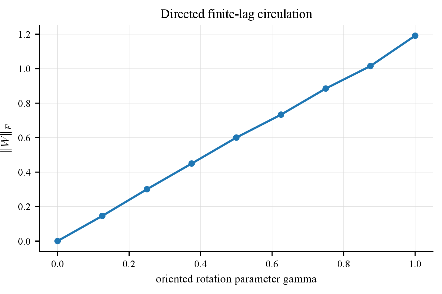
12.2 Affine covariance experiment↩︎
The affine covariance experiment uses a length-\(6\) cyclic-shift trajectory cloud in \(d=12\), with \(32\) trials and \(10\) time steps per trial. The empirical observables are computed at the dense median-heuristic bandwidth.
We run two versions. In the push-forward version, the dense source-smoothing weights are computed on the base cloud and then held fixed while the paired coordinates are transformed as \[(X,Y)\mapsto(AX+b,AY+b).\] This is the empirical analogue of pushing forward the conditional law in Theorem 1. In the re-kernelized version, the Euclidean Gaussian kernel is rebuilt after transforming the source coordinates. Under anisotropic transformations this changes the empirical conditional law, so the resulting values test estimator sensitivity rather than tensorial covariance.
| case | \(\operatorname{tr}(\bar G_\Delta)\) | spread trace | coherent trace | \(F_\Delta^\rho\) |
|---|---|---|---|---|
| base | \(1.000\) | \(1.000\) | \(1.000\) | \(0.523\) |
| orthogonal, \(M=I\) | \(1.000\) | \(1.000\) | \(1.000\) | \(0.523\) |
| scalar \(3I\), \(M=I\) | \(9.000\) | \(9.000\) | \(9.000\) | \(0.523\) |
| scalar \(3I\), \(M'=I/9\) | \(1.000\) | \(1.000\) | \(1.000\) | \(0.523\) |
| anisotropic re-kernelized, \(M=I\) | \(1.790\) | \(1.777\) | \(1.802\) | \(0.527\) |
| anisotropic re-kernelized, \(M'=A^{-\top}A^{-1}\) | \(1.002\) | \(0.999\) | \(1.004\) | \(0.525\) |
| anisotropic push-forward, \(M'=A^{-\top}A^{-1}\) | \(1.000\) | \(1.000\) | \(1.000\) | \(0.523\) |
Orthogonal transformations preserve Euclidean trace summaries. Scalar dilation rescales traces by \(3^2\), and the transformed metric restores the base values. In the anisotropic push-forward case, metric-corrected traces match the base values to numerical precision. In the re-kernelized anisotropic case, the corrected values remain close but not identical because the Gaussian source-smoothing operator has changed.
12.3 Dense stability experiment↩︎
The dense stability experiment perturbs a fixed normalized cyclic-shift trajectory cloud by additive Gaussian noise of scale \[\sigma_p\in\{0,10^{-4},3\cdot10^{-4},10^{-3},3\cdot10^{-3},10^{-2}, 3\cdot10^{-2}\}.\] The bandwidth is fixed to the base-cloud median-heuristic value. For each scale we average over eight perturbations and measure absolute changes in transport scale, coherent displacement trace, circulation norm, and dominant imaginary eigenvalue. Log-log slopes over the nonzero perturbation scales are \(1.16\), \(1.13\), \(1.07\), and \(1.01\), respectively, consistent with the Lipschitz behavior of Theorem 2.
| \(\sigma_p\) | \(\Delta\operatorname{tr}(\bar G_\Delta)\) | \(\Delta\) coherent trace | \(\Delta\|\mathcal W_\Delta\|_F\) | \(\Delta\omega_{\max}\) |
|---|---|---|---|---|
| \(10^{-4}\) | \(1.1{\times}10^{-5}\) | \(1.4{\times}10^{-5}\) | \(7.9{\times}10^{-7}\) | \(7.2{\times}10^{-7}\) |
| \(10^{-3}\) | \(1.1{\times}10^{-4}\) | \(1.1{\times}10^{-4}\) | \(1.3{\times}10^{-5}\) | \(1.0{\times}10^{-5}\) |
| \(10^{-2}\) | \(1.4{\times}10^{-3}\) | \(1.6{\times}10^{-3}\) | \(1.0{\times}10^{-4}\) | \(8.2{\times}10^{-5}\) |
| \(3{\times}10^{-2}\) | \(1.1{\times}10^{-2}\) | \(1.0{\times}10^{-2}\) | \(4.6{\times}10^{-4}\) | \(2.6{\times}10^{-4}\) |
12.4 Repeat-copy task and training protocol↩︎
All recurrent experiments use repeat-copy with feature dimension \(F=4\). Each sequence has a pattern phase, a delimiter, an optional blank delay, and a recall phase. For copy length \(L\), a pattern \[P\in\{-1,+1\}^{L\times F}\] is sampled uniformly. Inputs present the pattern for \(L\) steps, then a delimiter cue, then blank inputs. Targets are zero until the recall phase and then reproduce the pattern.
The five seed performance matched run and the dense sensitivity sweeps use the standard repeat-copy configuration with \(L=10\). The capacity-control and memory-horizon experiments use \(L=8\), as specified below. In all cases the geometry is computed on validation hidden trajectories after restoring the best validation-recall checkpoint.
We use three architectures. Elman is a tanh recurrent network (nn.RNN) with a linear readout. GRU is a standard nn.GRU with a linear readout. LSTM is a one-layer LSTM unrolled explicitly so that both hidden state \(h_t\) and cell state \(c_t\) are available as trajectories. For LSTM we report \(h_t\), \(c_t\), and the concatenation \((h_t,c_t)\) in the appendix.
Training uses a recall-window-weighted mean-squared loss: \[\mathcal{L} = \frac{1}{NTF} \sum_{n,t,f} w_t\bigl(\hat{y}_{n,t,f}-y_{n,t,f}\bigr)^2, \qquad w_t= \begin{cases} \lambda_{\rm recall}, & t\in \text{recall window},\\ 1, & \text{otherwise}, \end{cases}\] with \(\lambda_{\rm recall}=5.0\). Models are optimized with Adam. The five-seed performance-matched run uses hidden dimension \(64\), dense mode, center-RMS normalization, and architecture-specific optimization settings. Elman uses learning rate \(10^{-3}\) and \(120\) requested epochs. GRU and LSTM use learning rate \(3\cdot10^{-3}\) and \(240\) requested epochs.
The capacity-control experiment uses \(2048\) training sequences, \(256\) validation sequences, batch size \(64\), patience \(40\), minimum \(80\) epochs, and copy length \(L=8\). Elman uses \(120\) requested epochs, while GRU and LSTM use \(240\). The memory-horizon and phase-profile experiments use \(2048\) training sequences, \(192\) validation sequences, patience \(60\), minimum \(100\) epochs, copy length \(L=8\), and requested epoch budgets \(180\) for Elman and \(320\) for GRU/LSTM. The phase-profile experiment fixes delay \(D=4\) and computes separate phase-local operators on write, cue, delay, and recall source–successor pairs.
12.5 Operator estimation and baselines↩︎
For trained recurrent networks, validation hidden trajectories are pooled across sequences to form source–successor pairs. In the five-seed performance-matched and sensitivity runs, the pooled source set contains \(4864\) valid source nodes per run. The dense \(n\times n\) Gaussian kernel matrix is therefore manageable in memory. Local moments are computed in chunks to avoid materializing the full \((\text{chunk},n,d)\) displacement tensor.
The default bandwidth is \[\varepsilon_{\rm med} = \frac{1}{4}\operatorname{median}_{i<j}\|x_i-x_j\|^2,\] estimated from at most \(2000\) source states when the full source cloud is larger. The \(k\)-NN approximation of Appendix 7.6 is reported only in sensitivity studies.
For comparison, we compute several standard summaries on the same normalized hidden trajectories. Static effective rank is \[\exp\!\left(-\sum_i p_i\log p_i\right), \qquad p_i=\lambda_i/\sum_j\lambda_j,\] where \(\lambda_i\) are covariance eigenvalues. Dynamic mode decomposition fits \(Y\approx XA^\top\) by ridge regression with regularization \(10^{-4}\) and reports pooled validation-pair prediction \(R^2\). TICA reports eigenvalues of the symmetrized lagged covariance operator, and VAMP reports singular values of the whitened lagged cross-covariance, both with ridge regularization \(10^{-4}\). We also report relative lagged-covariance skew, \[\|C_{0t}-C_{0t}^\top\|_F/\|C_{0t}\|_F.\]
12.6 Resolution and \(k\)-NN sensitivity↩︎
The dense bandwidth sweep covers \[\varepsilon/\varepsilon_{\rm med} \in \{0.1,0.2,0.3,0.5,1.0,2.0\}\] on hidden states from the performance-matched repeat-copy case study. Table 5 reports coherent displacement fraction at \(\Delta=1\), center-RMS normalization, averaged over three seeds for the dense matched sensitivity run.
| state | \(0.1\) | \(0.2\) | \(0.3\) | \(0.5\) | \(1.0\) | \(2.0\) |
|---|---|---|---|---|---|---|
| Elman \(h\) | \(0.616\) | \(0.535\) | \(0.519\) | \(0.510\) | \(0.503\) | \(0.500\) |
| GRU \(h\) | \(0.528\) | \(0.472\) | \(0.453\) | \(0.445\) | \(0.454\) | \(0.469\) |
| LSTM \(h\) | \(0.581\) | \(0.508\) | \(0.522\) | \(0.520\) | \(0.502\) | \(0.493\) |
| LSTM \(c\) | \(0.548\) | \(0.485\) | \(0.488\) | \(0.489\) | \(0.486\) | \(0.486\) |
| LSTM \((h,c)\) | \(0.563\) | \(0.495\) | \(0.501\) | \(0.501\) | \(0.492\) | \(0.488\) |
The effective-neighborhood diagnostics confirm that the smallest dense bandwidth is not a self-loop artifact. At \(\varepsilon/\varepsilon_{\rm med}=0.1\), average self-mass over \(h\)-state runs is about \(0.09\) and the entropy-effective neighborhood size is about \(8.3\times10^2\). At the median bandwidth, self-mass is near zero and the effective neighborhood size is about \(4.6\times10^3\).
Whitening changes absolute trace scale and shifts coherent fractions. This is consistent with Theorem 1. Scalar trace summaries depend on the metric used to contract the transport tensor. We report center-RMS Euclidean summaries in the main text and use whitening as a sensitivity analysis.
At \(k=16\), the sparse approximation increases \(F_\Delta^\rho\) from roughly \(0.46\)–\(0.50\) for the dense estimator to roughly \(0.68\)–\(0.70\) across states, and increases circulation norms by about an order of magnitude. This confirms that hard sparse conditioning changes the local resolution, so we therefore use it only as a sensitivity analysis.
12.7 Performance matched repeat-copy details↩︎
| arch/state | recall MSE | sign acc. | \(\operatorname{tr}(\bar G_\Delta)\) | spread | coherent | \(F_\Delta^\rho\) |
|---|---|---|---|---|---|---|
| Elman \(h\) | \(0.0009\) | \(1.0000\) | \(1.008\) | \(1.002\) | \(1.015\) | \(0.503\) |
| GRU \(h\) | \(0.0006\) | \(1.0000\) | \(0.867\) | \(0.929\) | \(0.805\) | \(0.464\) |
| LSTM \(h\) | \(0.0010\) | \(0.9999\) | \(0.881\) | \(0.891\) | \(0.872\) | \(0.495\) |
| LSTM \(c\) | \(0.0010\) | \(0.9999\) | \(0.867\) | \(0.916\) | \(0.818\) | \(0.472\) |
| LSTM \((h,c)\) | \(0.0010\) | \(0.9999\) | \(0.876\) | \(0.911\) | \(0.840\) | \(0.480\) |
The main text reports \(h_t\) for architectural comparison. The additional LSTM rows show that \(h_t\), \(c_t\), and \((h_t,c_t)\) have distinct finite-lag geometry under the same estimator.
12.8 Capacity controls↩︎
The capacity-control experiment uses copy length \(L=8\) and sweeps \[\text{Elman-64},\;\text{Elman-128},\;\text{GRU-36},\;\text{GRU-64},\; \text{LSTM-32},\;\text{LSTM-64}.\] GRU-36 and LSTM-32 are approximate parameter-count controls for Elman-64. All configurations achieve near-perfect recall sign accuracy, although the smaller gated models have slightly larger recall MSE.
| config | params | recall MSE | sign acc. | \(\operatorname{tr}(\bar G_\Delta)\) | coherent trace | static rank |
|---|---|---|---|---|---|---|
| Elman-64 | \(4{,}804\) | \(0.0007\) | \(1.000\) | \(1.013\pm0.001\) | \(1.018\pm0.002\) | \(22.6\pm0.4\) |
| Elman-128 | \(17{,}796\) | \(0.0005\) | \(1.000\) | \(1.014\pm0.001\) | \(1.024\pm0.003\) | \(27.0\pm0.3\) |
| GRU-36 | \(4{,}792\) | \(0.0036\) | \(1.000\) | \(0.858\pm0.067\) | \(0.798\pm0.150\) | \(11.0\pm3.6\) |
| GRU-64 | \(13{,}892\) | \(0.0001\) | \(1.000\) | \(0.892\pm0.013\) | \(0.857\pm0.029\) | \(13.5\pm0.4\) |
| LSTM-32 | \(5{,}124\) | \(0.0029\) | \(1.000\) | \(0.886\pm0.005\) | \(0.892\pm0.019\) | \(11.1\pm0.9\) |
| LSTM-64 | \(18{,}436\) | \(0.0002\) | \(1.000\) | \(0.879\pm0.005\) | \(0.844\pm0.006\) | \(12.9\pm0.2\) |
The coherent displacement fraction is not a robust family separator in this sweep, as LSTM-32 has a fraction close to Elman despite lower transport scale. The more stable finite-lag distinctions are total transport scale and coherent displacement trace.
12.9 Phase-resolved repeat-copy profile↩︎
The phase-profile experiment localizes where finite-lag transport differences arise within a solved recurrent computation. We use repeat-copy with delay \(D=4\), copy length \(L=8\), hidden dimension \(64\), three seeds, dense mode, center-RMS normalization, lag \(\Delta=1\), and median-heuristic bandwidth. All \(h_t\) runs solve the task with recall sign accuracy \(1.0\).
We split source–successor pairs into task phases. The write phase contains source times receiving pattern inputs, the cue phase contains the delimiter transition, the delay phase contains blank-memory transitions, and the recall phase contains output transitions. We apply one global center-RMS normalization to the validation trajectory cloud, then build a separate dense phase-local operator for each phase. The cue phase has only one source time, so it is included as a transition diagnostic rather than a primary architecture-level conclusion.
| arch | phase | \(\operatorname{tr}(\bar G_\Delta)\) | coherent trace | static rank |
|---|---|---|---|---|
| Elman | write | \(0.841\) | \(0.859\) | \(8.7\) |
| Elman | cue | \(0.445\) | \(0.484\) | \(21.6\) |
| Elman | delay | \(0.583\) | \(0.495\) | \(27.4\) |
| Elman | recall | \(1.343\) | \(1.275\) | \(22.9\) |
| GRU | write | \(0.303\) | \(0.227\) | \(6.2\) |
| GRU | cue | \(0.213\) | \(0.298\) | \(19.0\) |
| GRU | delay | \(0.393\) | \(0.410\) | \(10.0\) |
| GRU | recall | \(0.602\) | \(0.623\) | \(11.3\) |
| LSTM | write | \(0.298\) | \(0.228\) | \(5.4\) |
| LSTM | cue | \(0.055\) | \(0.096\) | \(12.2\) |
| LSTM | delay | \(0.300\) | \(0.323\) | \(3.6\) |
| LSTM | recall | \(0.847\) | \(0.840\) | \(13.8\) |
The global transport-scale differences are concentrated in write and recall phases. Elman has substantially larger transport and coherent displacement during write and recall, while GRU and LSTM maintain lower transport through write, cue, and delay and increase at recall. Static rank follows a different pattern: for example, Elman has high static rank during delay, while its largest finite-lag transport occurs during recall. This illustrates the distinction between snapshot geometry and finite-lag transport geometry.
12.10 Memory-horizon experiment↩︎
The memory-horizon experiment inserts a blank delay \[D\in\{0,2,4,6,8\}\] between delimiter and recall. We use copy length \(L=8\), hidden dimension \(64\), three seeds, dense mode, center-RMS normalization, lag \(\Delta=1\), and median-heuristic bandwidth. Geometry is interpreted only on solved rows, defined by validation recall sign accuracy at least \(0.9\). GRU and LSTM solve all delays across all three seeds. Elman solves all seeds through \(D=6\) and two of three seeds at \(D=8\).
| architecture | \(D=0\) | \(D=2\) | \(D=4\) | \(D=6\) | \(D=8\) |
|---|---|---|---|---|---|
| Elman | \(1.000\) | \(1.000\) | \(1.000\) | \(0.997\) | \(0.950\) |
| GRU | \(1.000\) | \(1.000\) | \(1.000\) | \(1.000\) | \(1.000\) |
| LSTM | \(1.000\) | \(1.000\) | \(1.000\) | \(1.000\) | \(1.000\) |
| arch | delay | \(\operatorname{tr}(\bar G_\Delta)\) | coherent trace | \(F_\Delta^\rho\) | static rank |
|---|---|---|---|---|---|
| Elman | \(0\) | \(1.012\) | \(1.016\) | \(0.502\) | \(22.6\) |
| Elman | \(2\) | \(1.012\) | \(1.014\) | \(0.501\) | \(26.0\) |
| Elman | \(4\) | \(0.950\) | \(0.941\) | \(0.496\) | \(31.0\) |
| Elman | \(6\) | \(0.875\) | \(0.911\) | \(0.521\) | \(28.2\) |
| Elman | \(8\) | \(0.921\) | \(0.946\) | \(0.514\) | \(23.7\) |
| GRU | \(0\) | \(0.875\) | \(0.826\) | \(0.471\) | \(12.3\) |
| GRU | \(2\) | \(0.822\) | \(0.727\) | \(0.442\) | \(11.1\) |
| GRU | \(4\) | \(0.749\) | \(0.606\) | \(0.405\) | \(8.3\) |
| GRU | \(6\) | \(0.727\) | \(0.574\) | \(0.395\) | \(8.0\) |
| GRU | \(8\) | \(0.716\) | \(0.563\) | \(0.393\) | \(7.6\) |
| LSTM | \(0\) | \(0.880\) | \(0.842\) | \(0.478\) | \(13.0\) |
| LSTM | \(2\) | \(0.845\) | \(0.792\) | \(0.469\) | \(13.9\) |
| LSTM | \(4\) | \(0.786\) | \(0.665\) | \(0.423\) | \(10.1\) |
| LSTM | \(6\) | \(0.764\) | \(0.634\) | \(0.415\) | \(9.2\) |
| LSTM | \(8\) | \(0.728\) | \(0.640\) | \(0.439\) | \(10.0\) |
12.11 Compute and reproducibility↩︎
The dense estimator scales as \(O(n^2d)\) on \(n\) pooled source nodes. For the repeat-copy experiments, dense kernel matrices contain roughly \(5\times10^3\) source nodes and are feasible on a single workstation. Synthetic experiments run in seconds to minutes. The main repeat-copy and sensitivity experiments use five and three seeds, respectively, while capacity controls, memory-horizon experiments, and phase-profile experiments use three seeds.