Distributionally Robust Listwise Preference Optimization
July 02, 2026
Abstract
Existing robust preference optimization for language-model alignment mainly studies pairwise supervision and places robustness at the dataset, prompt, or preference-pair level. We instead study listwise preference optimization under ranking-label uncertainty: given a prompt and a candidate list, the observed ranking over that list may be ambiguous due to annotator inconsistency, near-ties, lossy rankwise feedback, or reward-model noise. We propose a pointwise total-variation robust Plackett–Luce objective that directly robustifies the ranking label conditional on the candidate list. The robust loss admits an exact decomposition into the nominal PL loss plus a worst-case PL correction, and the worst-case ranking is obtained by sorting current implicit scores in ascending order, reducing the inner maximization from \(K!\) enumeration to \(O(K\log K)\). This tractable structure yields strong offline and online optimization guarantees. In the offline fixed-list setting, the robust objective is convex and projected stochastic subgradient reaches global \(\epsilon\)-suboptimality with \(O(\epsilon^{-2})\) sample complexity. In the online policy-induced setting, where candidate lists are generated by the current policy, we establish weak convexity and \(\widetilde{O}(\epsilon^{-2})\) Moreau-envelope stationarity. Experiments in offline LLM alignment show that the proposed robust correction largely preserves performance under clean labels and improves robustness under noise. In online alignment, it makes reward-model-ranked candidate expansion more reliable and improves both reward-model and external GPT-4 judge metrics.
1 Introduction↩︎
Learning from human preferences has become a central mechanism for aligning large language models, with reinforcement-learning-from-human-feedback (RLHF) and direct preference optimization (DPO) serving as standard recipes for instruction-tuned models [1]–[3]. Most existing analyses and algorithms formulate preference feedback as pairwise supervision under a Bradley–Terry (BT) model [3], [4], where each training example identifies a chosen response and a rejected response. However, many modern preference datasets are naturally listwise: for a single prompt, multiple candidate responses are available, and the supervision may contain a full or partial ranking. This has motivated Plackett–Luce (PL) listwise preference objectives [5]–[8], which exploit the relative ordering of multiple candidates rather than reducing the feedback to isolated pairwise comparisons.
While these works establish listwise preference optimization, they do not address robustness to uncertainty in the observed ranking label itself. To the best of our knowledge, this is the first work to study robust listwise preference optimization for LLM alignment under conditional ranking-label ambiguity.
Robust preference optimization has developed largely along a different axis. Recent robust DPO-style methods introduce distributional uncertainty over the empirical preference dataset, the prompt distribution, or the preference-pair distribution [9]–[11]. These approaches address an important question: how should alignment behave when the distribution from which prompts or preference pairs are sampled is perturbed? They do not directly address a different and common source of uncertainty in listwise supervision: even after conditioning on the same prompt and the same candidate list, the observed ranking label itself may be unreliable.
This paper studies this conditional ranking-label uncertainty. Given a prompt \(x\), a realized candidate list \(Y=(y_1,\ldots,y_K)\), and an observed ranking \(\sigma^\star\), we allow the ranking-label distribution to vary within a pointwise total-variation ambiguity set around the empirical ranking. This models local ambiguity caused by annotator inconsistency, near-ties between candidates, tied or lossy rankwise feedback, and reward-model-induced ranking noise in online alignment. The key distinction from prior robust preference-optimization work is that we do not robustify which prompts, pairs, or candidate lists are sampled; instead, conditional on a realized candidate list, we robustify the ranking label over that list.
This candidate-list-conditioned formulation has two advantages. First, it targets the supervision noise directly: for a fixed prompt–candidate-list instance, annotator disagreement, reward-model errors, near-ties, and lossy rank annotations all manifest as uncertainty in the observed ordering among the same alternatives.
Second, the formulation preserves the full listwise ranking signal. The PL model is a strict listwise generalization of the pairwise BT/DPO objective: when \(K=2\), it recovers the standard pairwise preference loss, while for \(K>2\), it retains the sequence-level ordering among multiple candidates. Prior listwise ranking and preference-optimization methods have shown that using the relative ordering among multiple candidates can exploit richer supervision than reducing feedback to isolated pairwise comparisons [6]–[8]. Our robustification keeps this listwise structure intact: it perturbs the ranking over the same candidate set rather than decomposing the supervision into independent pairwise label flips.
At first glance, this formulation appears computationally expensive because the adversary may choose among \(K!\) possible rankings. Our main structural observation is that the PL loss makes this inner maximization exactly tractable: the worst-case ranking is obtained by sorting the current implicit scores in ascending order. Consequently, the robust listwise loss reduces to a convex combination of the nominal PL loss and a single adversarial PL loss, computable in \(O(K\log K)\) time. For \(K\ge 3\), this correction is intrinsically listwise and does not reduce to a collection of independent pairwise BT corrections.
We analyze the resulting objective in both offline and online settings naturally induced by listwise alignment. In the offline fixed-list setting with log-linear scores, the robust objective is convex and reaches global \(\epsilon\)-suboptimality with \(O(\epsilon^{-2})\) sample complexity. In the online policy-induced setting, where candidate lists are sampled from the current policy, the objective is no longer globally convex; we establish weak convexity and an \(\widetilde{O}(\epsilon^{-2})\) Moreau-envelope stationarity guarantee using an explicit ascending-sort Clarke-subgradient oracle. Empirically, the proposed correction behaves as a conservative ranking-label regularizer: it preserves clean-label performance, improves stability under structured ranking-label corruption, and helps larger listwise candidate sets become more reliable in online reward-model-driven alignment.
1.1 Contributions↩︎
Our contributions are as follows.
A robust listwise preference-optimization formulation. To the best of our knowledge, we are the first to study robust listwise preference optimization for LLM alignment under conditional ranking-label uncertainty. Unlike prior robust DPO methods that perturb the data, prompt, or pair distribution, our ambiguity set targets the ranking label conditional on a realized candidate list. The formulation recovers the standard pairwise BT/DPO setting when \(K=2\), while providing a genuinely listwise robustness model when \(K>2\).
Exact and tractable robust PL loss. We show that the robust PL loss admits an exact decomposition into the nominal PL loss and a worst-case PL loss. Although the inner maximization is over \(K!\) rankings, the PL structure implies that the worst-case ranking is simply the ascending-score order, giving an \(O(K\log K)\) evaluation algorithm.
Strong offline and online optimization theory. In the offline fixed-list log-linear setting, the robust objective is convex and admits an \(O(\epsilon^{-2})\) stochastic subgradient guarantee. In the online policy-induced setting, we prove weak convexity and an \(\widetilde{O}(\epsilon^{-2})\) Moreau-envelope stationarity bound using an explicit Clarke-subgradient oracle. These guarantees improve or match closely related robust preference-optimization rates under comparable log-linear oracle models, as summarized in Table 1.
Empirical validation under ranking-label uncertainty. Offline experiments show that robust PL is most useful when listwise labels are structurally corrupted, especially under severe top-rank noise. Online LLM alignment experiments show that robustness helps larger candidate lists become more reliable when rankings are generated by a reward model.
1.2 Relation to Prior Robust Preference Optimization↩︎
Prior robust preference-optimization methods mainly study pairwise BT/DPO objectives and place robustness on the data, prompt, pair, or oracle distribution. In contrast, we study PL listwise preference optimization and place uncertainty on the ranking label conditional on a realized candidate list. This distinction is central: for \(K\ge 3\), our robust correction is a genuinely listwise PL max-gap over permutations, with an exact ascending-score solution rather than a reduction to independent pairwise BT corrections.
1 summarizes how our setting differs from representative robust preference-optimization theories in terms of preference model, robustness source, robust loss structure, and sample/oracle complexity. Additional discussion is provided in Appendix 8.
| Aspect | Distributionally Robust DPO [10] | Oracle-robust online alignment [12] | Ours |
|---|---|---|---|
| Preference model | Pairwise BT | Pairwise BT | PL rankings, including BT as \(K=2\) |
| Robustness source | Data / prompt distribution shift | Pairwise oracle perturbation | Ranking-label perturbation |
| Robust loss structure | Reweighting-based robust objective | Exact pairwise sensitivity penalty | Exact listwise sensitivity penalty, including pairwise as \(K=2\) |
| Log-linear policy class | Yes | Yes | Yes |
| Main guarantee | Offline robust DPO: \(nT=\tilde O(\varepsilon^{-4})\) | Online Moreau stationarity: \(\tilde O(\varepsilon^{-2})\) | Offline: \(B_sT=O(\varepsilon^{-2})\); Online: \(\tilde O(\varepsilon^{-2})\) Moreau stationarity |
| Empirical setting | Offline | - | Offline and online |
5pt

2 Background: From Pairwise DPO to Listwise PL-DPO↩︎
Given a prompt \(x\) and two responses \(y^+,y^-\), the Bradley–Terry (BT) model assumes \(\mathbb{P}(y^+\succ y^-\mid x) = \sigma\!\big(r^\star(x,y^+)-r^\star(x,y^-)\big)\), where \(\sigma\) is the logistic sigmoid and \(r^\star\) is the latent ground-truth reward [4]. Under KL-regularized RLHF the optimal policy admits the Gibbs form \(\pi^\star(y\mid x)\propto\pi_{\mathrm{ref}}(y\mid x)\exp(r^\star(x,y)/\beta)\), so \(r^\star(x,y)=\beta\log[\pi^\star(y\mid x)/\pi_{\mathrm{ref}}(y\mid x)]+\beta\log Z(x)\). The partition \(\beta\log Z(x)\) cancels in the BT difference, motivating the implicit DPO score \(g_\theta(x,y):=\beta\log[\pi_\theta(y\mid x)/\pi_{\mathrm{ref}}(y\mid x)]\) and the pairwise DPO loss \(\ell_{\mathrm{DPO}}(\theta;x,y^+,y^-) = -\log\sigma(g_\theta(x,y^+)-g_\theta(x,y^-))\) [3].
2.0.0.1 Listwise generalization via Plackett–Luce.
For each prompt \(x\), suppose we observe a realized candidate list \(\mathcal{Y}=\{y_1,\dots,y_K\}\) and a deterministic empirical ranking \(\sigma^\star\in S_K\), where \(\sigma^\star_i\) is the index of the response placed at rank \(i\). The listwise analogue of BT is the Plackett–Luce model [5]: \[\mathbb{P}(\sigma^\star\mid x,\mathcal{Y}) = \prod_{i=1}^K \frac{\exp(r^\star(x,y_{\sigma^\star_i}))}{\sum_{j=i}^K \exp(r^\star(x,y_{\sigma^\star_j}))}. \label{eq:pl-prob}\tag{1}\] Substituting the same DPO reparameterization, the partition \(\beta\log Z(x)\) cancels at every stage of the product, yielding the listwise PL-DPO loss \[\ell_{\mathrm{PL}}(\theta;x,y_{1:K},\sigma) = -\sum_{i=1}^K g_\theta(x,y_{\sigma_i}) + \sum_{i=1}^K \log\!\Big(\sum_{j=i}^K \exp(g_\theta(x,y_{\sigma_j}))\Big). \label{eq:pl-loss}\tag{2}\] At \(K=2\) and \(\sigma=(1,2)\), 2 reduces to \(-\log\sigma(g_\theta(x,y_1)-g_\theta(x,y_2))\), recovering pairwise DPO exactly. For \(K\ge 3\), \(\ell_{\mathrm{PL}}\) aggregates information from \(K-1\) stagewise PL choices and is strictly more informative than any single pairwise comparison drawn from the same list. A formal curvature view of this stagewise information aggregation is provided in 4.
The nominal listwise objective on a fixed offline dataset \(\mathcal{D}=\{(x,y_{1:K},\sigma^\star)\}\) is \(J_{\mathrm{nom}}(\theta) := \mathbb{E}_{(x,y_{1:K},\sigma^\star)\sim\mathcal{D}}[\ell_{\mathrm{PL}}(\theta;x,y_{1:K},\sigma^\star)]\). We add ranking-label robustness next.
3 Pointwise TV-Robust Listwise Objective↩︎
We treat each empirical ranking label \(\sigma^\star\) as a Dirac point mass on \(S_K\) and let an adversary perturb this label distribution within a TV ball of radius \(\rho\in[0,1]\).
Definition 1 (Pointwise TV ambiguity). For sample \((x,y_{1:K},\sigma^\star)\), \[\mathcal{U}_{\mathrm{TV}}(\delta_{\sigma^\star},\rho) := \big\{P\in\Delta(S_K):\mathrm{TV}(P,\delta_{\sigma^\star})\le\rho\big\}, \quad \mathrm{TV}(P,Q)=\tfrac12\|P-Q\|_1. \label{eq:tv-set}\tag{3}\]
Definition 2 (Robust listwise objective). The pointwise robust loss and offline robust objective are \[\begin{align} \ell_{\mathrm{rob}}(\theta;x,y_{1:K},\sigma^\star) &:= \max_{P\in\mathcal{U}_{\mathrm{TV}}(\delta_{\sigma^\star},\rho)} \mathbb{E}_{\sigma\sim P}[\ell_{\mathrm{PL}}(\theta;x,y_{1:K},\sigma)], \notag \\ J_{\mathrm{rob}}(\theta) &:= \mathbb{E}_{\mathcal{D}}[\ell_{\mathrm{rob}}(\theta;x,y_{1:K},\sigma^\star)]. \label{eq:robust-loss} \end{align}\tag{4}\]
Lemma 1 (Exact pointwise TV decomposition). For every sample \((x,y_{1:K},\sigma^\star)\), parameter \(\theta\), and \(\rho\in[0,1]\), \[\ell_{\mathrm{rob}}(\theta;x,y_{1:K},\sigma^\star) = (1-\rho)\,\ell_{\mathrm{PL}}(\theta;x,y_{1:K},\sigma^\star) + \rho\max_{\sigma\in S_K}\ell_{\mathrm{PL}}(\theta;x,y_{1:K},\sigma). \label{eq:tv-decomp}\tag{5}\] Equivalently, \(\ell_{\mathrm{rob}} = \ell_{\mathrm{PL}}(\sigma^\star)+\rho\big(\max_\sigma\ell_{\mathrm{PL}}(\sigma)-\ell_{\mathrm{PL}}(\sigma^\star)\big)\).
The full proof is in Appendix 10.
4 Tractable Worst-Case Ranking↩︎
By 1, evaluating the pointwise robust loss requires solving \[\max_{\sigma\in S_K}\ell_{\mathrm{PL}}(\theta;x,y_{1:K},\sigma),\] which is naively a maximization over \(K!\) possible rankings. The key structural observation is that, under the PL loss, the adversarial ranking is not arbitrary: it is obtained by placing low-score candidates before high-score candidates. Thus the inner maximization reduces to a single sorting operation.
Theorem 1 (Worst-case ranking by ascending scores). Fix \((\theta,x,y_{1:K})\) and let \(g_i:=g_\theta(x,y_i)\). If \(\sigma_{\rm wc}\in S_K\) sorts the scores in nondecreasing order, \(g_{\sigma_{\rm wc}(1)}\le \cdots \le g_{\sigma_{\rm wc}(K)}\), then \[\sigma_{\rm wc}\in \arg\max_{\sigma\in S_K} \ell_{\mathrm{PL}}(\theta;x,y_{1:K},\sigma).\] Hence the inner maximization in the robust PL loss is solved by sorting and costs \(O(K\log K)\). With ties, any deterministic tie-breaking rule within tied groups is valid.
The full proof is in Appendix 11.

Figure 2: 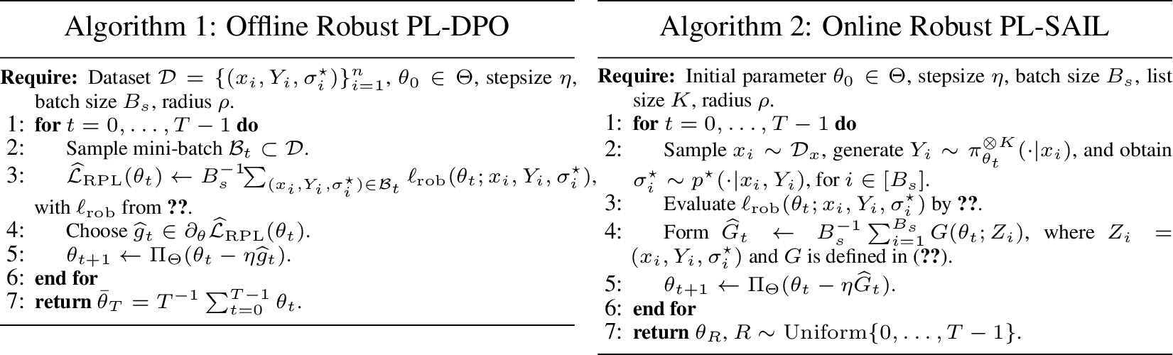 .
.
5 Optimization Theory↩︎
We analyze two settings: an offline fixed-list setting in which \((y_{1:K},\sigma^\star)\) is independent of \(\theta\), and an online policy-induced setting in which \(Y\) is sampled from the current policy \(\pi_\theta^{\otimes K}\).
The offline and online optimization procedures are summarized in [alg:offline-robust-pl-dpo,alg:online-robust-pl-sail].
5.1 Offline Fixed-List Setting↩︎
Assumption 1 (Log-linear policy class). The response space \(\mathcal{Y}\) is finite. Let \(\psi:\mathcal{X}\times\mathcal{Y}\to\mathbb{R}^{d_p}\) satisfy \(\sup_{x,y}\|\psi(x,y)\|_2\le B_\psi\), where \(B_\psi=1\) can be obtained by rescaling. For \(B>0\), let \(\Theta:=\{\theta\in\mathbb{R}^{d_p}:\|\theta\|_2\le B\}\), and consider \[\Pi = \left\{ \pi_\theta: \pi_\theta(y|x) = \frac{\exp(\theta^\top\psi(x,y))}{\sum_{y'\in\mathcal{Y}}\exp(\theta^\top\psi(x,y'))}, \;\theta\in\Theta \right\}.\] Assume \(\pi_{\rm ref}=\pi_{\theta_{\rm ref}}\) for some fixed \(\theta_{\rm ref}\in\Theta\), and set \(D:=\sup_{\theta\in\Theta}\|\theta-\theta_{\rm ref}\|_2<\infty\).
Remark 1 (On the log-linear policy class assumption). The log-linear policy assumption is a standard simplification in theoretical analyses of reinforcement learning [13], [14], RLHF [15], and DPO [16]. Closely related robust-alignment works also adopt log-linear policy assumption, including the online oracle-robust alignment setting of [12], the offline Distributionally Robust DPO setting of [10], and distributionally robust DPO variants such as WDPO/KLDPO [11]. We use this assumption to isolate the optimization structure of the proposed robust listwise objective.
Proposition 1 (Convexity of the offline robust objective). Suppose 1 holds, \(\theta\mapsto\ell_{\mathrm{PL}}(\theta;x,y_{1:K},\sigma)\) is convex for every \((x,y_{1:K},\sigma)\). Hence by 1, \(\theta\mapsto\ell_{\mathrm{rob}}(\theta;x,y_{1:K},\sigma^\star)\) is convex on \(\Theta\). The offline robust objective \(J_{\mathrm{rob}}\) is convex.
The proof is in Appendix 12.1. We use the projected stochastic subgradient method \[\theta_{t+1} = \Pi_\Theta\big(\theta_t - \eta\,\widehat g_t\big),\qquad t=0,\dots,T-1, \label{eq:proj-subgrad}\tag{6}\] where \(\widehat g_t\) is a mini-batch unbiased subgradient estimator with conditional variance bounded by \(\sigma_g^2/B_s\) (mini-batch size \(B_s\)).
Theorem 2 (Offline suboptimality of projected stochastic subgradient). Suppose 1 holds, a mini-batch oracle with second moment bounded as \(\mathbb{E}[\|\widehat g_t\|_2^2\mid\theta_t]\le 4K^2B_\psi^2+\sigma_g^2/B_s\), with \(\eta = 2B/\sqrt{T(4K^2B_\psi^2+\sigma_g^2/B_s)}\) the averaged iterate \(\bar\theta_T:=\tfrac1T\sum_{t=0}^{T-1}\theta_t\) satisfies \[\mathbb{E}[J_{\mathrm{rob}}(\bar\theta_T)] - \min_{\theta\in\Theta} J_{\mathrm{rob}}(\theta) \le \frac{2B\sqrt{4K^2B_\psi^2+\sigma_g^2/B_s}}{\sqrt{T}}. \label{eq:offline-rate}\tag{7}\] Consequently \(T = O((4K^2B_\psi^2+\sigma_g^2/B_s)/\varepsilon^2)\) iterations suffice for \(\varepsilon\)-suboptimality. With fixed \(B_s=\Theta(1)\), the total sample complexity is \(B_s T=O(\varepsilon^{-2})\).
The full proof is in Appendix 12.3.
Remark 2 (Comparison with prior robust DPO theory). 2 is most directly comparable to the DPO-side rate in offline Distributionally Robust DPO [10]. The robustness source is different: Distributionally Robust DPO considers distributional robustness over the data or prompt distribution, whereas our method considers pointwise ranking-label robustness on a realized candidate list. This difference leads to different total sample/oracle complexities. In [10], the DPO-side guarantee uses \(T=O(\varepsilon^{-2})\) iterations and a minibatch size satisfying \(n/\log n=\Omega(\varepsilon^{-2})\), leading to total sample complexity \(nT=\tilde{O}(\varepsilon^{-4})\). In contrast, our explicit listwise robust oracle yields \(T=O(\varepsilon^{-2})\), \(B_sT=O(\varepsilon^{-2})\) when the minibatch size is fixed as \(B_s=\Theta(1)\). Thus, under our bounded second-moment oracle model, the offline listwise robust objective admits a cleaner \(O(\varepsilon^{-2})\) sample/oracle complexity.
Remark 3 (Optimality under the current model). This \(O(T^{-1/2})\) rate is the standard stochastic subgradient rate for nonsmooth convex objectives; faster rates would require additional smoothness, curvature, or non-degeneracy assumptions that stabilize the active worst-case ranking.
5.2 Online Policy-Induced Setting↩︎
We now study the on-policy setting where, for each prompt \(x\sim\mathcal{D}_x\), the candidate list \(Y=(y_1,\dots,y_K)\in\mathcal{Y}^K\) is sampled iid as \(Y\sim\pi_\theta^{\otimes K}(\cdot\mid x)\). The ranking oracle returns \(\sigma^\star\sim p^\star(\cdot\mid x,Y)\), conditionally independent of \(\theta\) given \((x,Y)\). Notation: in the offline log-linear setting (5.1) we wrote scores as \(g_\theta(x,y)=\theta^\top\phi(x,y)\). In the online setting we instead parameterize the policy as \(\pi_\theta(y\mid x)\propto\exp(\theta^\top\psi(x,y))\) and let \(s_\theta(x,y):=\log[\pi_\theta(y\mid x)/\pi_{\mathrm{ref}}(y\mid x)]\) be the induced log-ratio score. Both reduce to affine functions of \(\theta\). The online objectives are \[J_{\mathrm{nom}}^{\mathrm{on}}(\theta) := \mathbb{E}_{x,Y\sim\pi_\theta^{\otimes K},\sigma^\star\sim p^\star}[\ell_{\mathrm{PL}}(\theta;x,Y,\sigma^\star)], \quad J_{\mathrm{rob}}^{\mathrm{on}}(\theta) := \mathbb{E}_{x,Y\sim\pi_\theta^{\otimes K},\sigma^\star\sim p^\star}[\ell_{\mathrm{rob}}(\theta;x,Y,\sigma^\star)]. \label{eq:online-objectives}\tag{8}\] By 1, \(J_{\mathrm{rob}}^{\mathrm{on}}=J_{\mathrm{nom}}^{\mathrm{on}}+\rho A(\theta)\) with \(A(\theta)=\mathbb{E}\big[\max_\sigma\ell_{\mathrm{PL}}(\theta;x,Y,\sigma)-\ell_{\mathrm{PL}}(\theta;x,Y,\sigma^\star)\big]\). This connects the SAIL-style bilevel formulation of online alignment [17] with our pointwise-TV listwise robustness; see 14 for the bilevel-to-single-level reduction we use.
Because \(\pi_\theta^{\otimes K}\) depends on \(\theta\), \(J_{\mathrm{rob}}^{\mathrm{on}}\) is not globally convex in general. Our analysis therefore departs from the offline case: we work in the weakly convex framework [18], [19], with the Clarke subdifferential \(\partial_C\) [20].
Assumption 2 (Online policy-induced sampling and well-posedness). For each \(\theta\in\Theta\), draw \(x\sim\mathcal{D}_x\), sample \(Y=(y_1,\ldots,y_K)\sim\pi_\theta^{\otimes K}(\cdot|x)\), and draw \(\sigma^\star\sim p^\star(\cdot|x,Y)\), where \(\mathcal{D}_x\) is independent of \(\theta\) and \(\sigma^\star\) is conditionally independent of \(\theta\) given \((x,Y)\). Define \[F(\theta):=J_{\rm rob}^{\rm on}(\theta)+I_\Theta(\theta),\qquad I_\Theta(\theta)= \begin{cases} 0,&\theta\in\Theta,\\ +\infty,&\theta\notin\Theta, \end{cases} \qquad F_{\inf}:=\inf_{\theta\in\mathbb{R}^{d_p}}F(\theta)>-\infty .\] Assume \(F\) is proper and lower semicontinuous and bounded below.
We do not place the existence of a Clarke-subdifferential stochastic oracle as an assumption; instead we construct one from ascending-sort below.
Proposition 2 (Online weak convexity). Suppose 1 2 hold. \(J_{\mathrm{rob}}^{\mathrm{on}}\) is \(\kappa\)-weakly convex on \(\Theta\) with \[\kappa = K^2 B_\psi^2\big(8 + \log K + 2DB_\psi\big). \label{eq:kappa-listwise}\qquad{(1)}\]
The bound ?? is polynomial in \(K\) and the model-boundedness constants; the full argument is deferred to Appendix 13.
5.2.0.1 Stochastic oracle from ascending-sort.
Let \(\sigma^{\mathrm{sel}}(\theta;x,Y)\) be the deterministic ascending-score maximizer of \(\ell_{\mathrm{PL}}(\theta;x,Y,\sigma)\), with fixed tie-breaking, as given by 1. For \(Z=(x,Y,\sigma^\star)\), define \[G(\theta;Z) := (1-\rho)\nabla\ell_{\mathrm{PL}}(\theta;x,Y,\sigma^\star) +\rho\nabla\ell_{\mathrm{PL}}(\theta;x,Y,\sigma^{\mathrm{sel}}) +\ell_{\mathrm{rob}}(\theta;x,Y,\sigma^\star)S_\theta(x,Y). \label{eq:oracle}\tag{9}\] The last term is the score-function correction for policy-induced sampling. 10 verifies that \(G\) is a valid stochastic Clarke-subgradient oracle with bounded second moment.
Theorem 3 (Online robust convergence). Suppose 1 2 hold. Let \(\kappa\) be as in ?? and \(G_{\mathrm{tot}}^2\) as in 15 . For \(F=J_{\mathrm{rob}}^{\mathrm{on}}+I_\Theta\) and \(\hat{\lambda}\in(0,1/\kappa)\), define \(F_{\hat{\lambda}}(\theta)=\min_{u\in\Theta}\{J_{\mathrm{rob}}^{\mathrm{on}}(u)+\tfrac1{2\hat{\lambda}}\|u-\theta\|^2\}\). Fix \(\hat{\lambda}\in(0,1/\kappa)\) and set \(\Delta_0:=F_{\hat{\lambda}}(\theta_0)-F_{\inf}\). Run [alg:online-robust-pl-sail] with the explicit ascending-sort oracle 9 and constant stepsize \(\eta=\sqrt{2\hat{\lambda}\Delta_0/(G_{\mathrm{tot}}^2 T)}\). Then \[\mathbb{E}\!\big[\|\nabla F_{\hat{\lambda}}(\theta_R)\|^2\big] \le \frac{2}{1-\kappa\hat{\lambda}}\sqrt{\frac{2\,\Delta_0\,G_{\mathrm{tot}}^2}{\hat{\lambda}\,T}}. \label{eq:online-rate}\tag{10}\]
Corollary 1 (Sample / oracle complexity). \(\mathbb{E}\|\nabla F_{\hat{\lambda}}(\theta_R)\|^2\le\varepsilon\) holds for \(T\ge 8\Delta_0 G_{\mathrm{tot}}^2/[\hat{\lambda}(1-\kappa\hat{\lambda})^2\varepsilon^2]\). At \(\hat{\lambda}=1/(2\kappa)\), \[T = O\!\left(\frac{\kappa\,\Delta_0\,G_{\mathrm{tot}}^2}{\varepsilon^2}\right) \;=\; \tilde{O}\!\left(\frac{K^6 B_\psi^4(\log K+DB_\psi)^3}{\varepsilon^2}\right). \label{eq:online-complexity}\tag{11}\]
The proofs of [thm:online-rate,cor:complexity] are in Appendix 13.
Remark 4 (Comparison with oracle-robust online alignment [12]). 3 matches the \(\tilde{O}(\varepsilon^{-2})\) Moreau-stationarity order of [12], but for a different robust object: they study pairwise BT oracle perturbations, while we study listwise PL ranking-label perturbations, with BT recovered at \(K=2\). Moreover, in our finite-response log-linear setting, the required PL bounds, score-function bounds, weak-convexity constant, and stochastic Clarke oracle are derived explicitly from the listwise structure rather than postulated as abstract regularity/oracle assumptions in [12].
6 Experiments↩︎
6.0.0.1 Evaluation questions.
Our experiments test the behavior predicted by the proposed ambiguity model rather than claiming that robustness monotonically improves all metrics. We ask whether the robust correction: (i) preserves performance when rankings are reliable; (ii) reduces the failure modes of PL learning when listwise labels are corrupted; and (iii) makes larger candidate lists more reliable in online alignment, where rankings are generated by a reward model.
We evaluate the proposed pointwise-TV robust PL objective in two settings matching our theory: offline fixed-list ranking with corrupted labels, and online policy-induced alignment with reward-model-generated rankings. Full experimental details are deferred to Appendix 17.
We provide anonymized code repositories for the online and offline experiments at https://anonymous.4open.science/r/robust-listwise-online-09BB and https://anonymous.4open.science/r/robust-listwise-offline-7FF6, respectively.
6.0.0.2 Setup.
We use UltraFeedback [21], where each prompt has four candidate responses, yielding a natural listwise preference problem with \(K=4\). We compare three objectives: Nominal BT, the standard pairwise DPO/BT baseline using chosen–rejected comparisons; Nominal PL, the non-robust listwise Plackett–Luce objective; and Robust PL, our pointwise-TV robust version of the PL objective. In the online setting, candidate responses are generated by the current policy and ranked by a frozen reward model; the corresponding evaluation metrics are defined in the online result table.
6.1 Offline fixed-list evaluation↩︎
The offline setting directly matches our ambiguity model: the prompt and candidate list are fixed, while the ranking label may be corrupted. Since binary chosen–rejected label flipping has no unique canonical analogue for a full ranking, we introduce two listwise corruptions. Near-tie corruption swaps the adjacent pair with the closest annotation scores, modeling local ambiguity between nearly indistinguishable responses. Top-rank corruption promotes a lower-ranked response to the first position, modeling a more severe error because the first PL stage selects from the full candidate list. The noise level \(\epsilon\) is the fraction of corrupted training rankings; evaluation labels are always clean.
We also include two pairwise robust-DPO baselines, TV-DR-DPO [10] and KLDPO [11], reimplemented in the same pipeline using their loss-level robust DPO objectives. Their hyperparameters are selected from held-out sweeps, with the sweep results reported in Appendix 16.2. We evaluate all methods by Kendall’s \(\tau\) on clean held-out rankings. Each method assigns scalar scores to the four candidate responses, which induce a predicted ranking; Kendall’s \(\tau\) measures the rank correlation with the clean UltraFeedback reference ranking.
6.1.0.1 Offline observations.
2 shows that Robust PL incurs only a small degradation under clean labels while providing clear gains when the ranking labels are corrupted. The improvement is most pronounced under severe top-rank corruption: when \(\epsilon=1.0\), Robust PL substantially improves over Nominal PL for both Qwen3-0.6B and Qwen3-8B. This matches the PL structure: top-rank errors corrupt the early stagewise choices that dominate the likelihood, whereas near-tie corruption often preserves much of the global ordering. Thus, in the offline fixed-list setting, Robust PL behaves as a conservative ranking-label regularizer: it largely preserves clean-label ranking performance while improving robustness to structured listwise label noise.
Appendix 16 provides further support: additional clean-label metrics show limited performance degradation, \(\rho\)-sweeps validate the robustness–over-regularization tradeoff, and Qwen2.5-0.5B/7B results show consistent trends across model families.
| Model | Noise condition | Nominal BT (DPO) | TV-DR-DPO \((\rho=0.10)\) | KLDPO \((\tau=1.00)\) | Nominal PL | Robust PL \((\rho=0.05)\) | Robust PL \((\rho=0.10)\) |
|---|---|---|---|---|---|---|---|
| Qwen3-0.6B | Clean | 0.298 | 0.282 | 0.277 | 0.288 | 0.276 | 0.284 |
| near_tie, \(\epsilon=0.4\) | 0.266 | 0.270 | 0.267 | 0.268 | 0.274 | 0.264 | |
| near_tie, \(\epsilon=1.0\) | 0.261 | 0.244 | 0.246 | 0.244 | 0.262 | 0.246 | |
| top_rank, \(\epsilon=0.4\) | 0.244 | 0.229 | 0.263 | 0.243 | 0.251 | 0.236 | |
| top_rank, \(\epsilon=1.0\) | 0.036 | 0.024 | 0.031 | 0.119 | 0.154 | 0.116 | |
| Qwen3-8B | Clean | 0.316 | 0.338 | 0.331 | 0.362 | 0.347 | 0.340 |
| near_tie, \(\epsilon=0.4\) | 0.291 | 0.319 | 0.318 | 0.348 | 0.356 | 0.333 | |
| near_tie, \(\epsilon=1.0\) | 0.281 | 0.310 | 0.310 | 0.322 | 0.327 | 0.319 | |
| top_rank, \(\epsilon=0.4\) | 0.302 | 0.282 | 0.296 | 0.321 | 0.329 | 0.293 | |
| top_rank, \(\epsilon=1.0\) | 0.039 | -0.056 | -0.016 | 0.103 | 0.146 | 0.076 |
6.2 Online policy-induced alignment↩︎
We next evaluate the online setting, where the current policy generates candidate responses and a frozen reward model ranks them to provide the training signal. This setting naturally introduces ranking-label uncertainty: increasing the list size from \(K=2\) to \(K=4\) provides richer preference information, but also requires the reward model to make finer-grained comparisons over more candidates. Thus, larger \(K\) is not automatically beneficial.
Our method is a robust listwise extension of the SAIL-style online preference-optimization pipeline. We therefore use the setting-matched binary SAIL baseline, recovered by \(K=2,\rho=0\). The non-robust listwise extension is \(K=4,\rho=0\), while \(\rho>0\) isolates the effect of the proposed robust ranking-label correction. We do not include PPO-style online RLHF or offline robust-DPO baselines as direct comparisons because they optimize different signals or robustify different objects. For external evaluation, we follow the LLM-as-a-judge protocol [22] and use GPT-4 [23] as the judge to compare model outputs against the dataset chosen responses.
6.2.0.1 Online observations.
3 shows that simply increasing the candidate-list size is not sufficient. The non-robust listwise variant \(K=4,\rho=0\) does not consistently improve over the binary baseline \(K=2,\rho=0\), suggesting that larger lists provide richer preference information but also introduce finer-grained reward-model ranking noise. Robustness mitigates this issue. With \(\rho>0\), the \(K=4\) variants become more reliable: for Qwen3-0.6B, \(K=4,\rho=0.02\) gives the best reward-model preference and GPT-4 judge scores; for Qwen3-8B, robust \(K=4\) variants achieve the strongest reward-model performance and ranking-agreement metrics. These results support our main interpretation that Robust PL helps convert larger candidate lists from a noisier supervision source into useful listwise preference signal. The GPT-4 judge gains further suggest that the improvement transfers beyond the reward model used for training.
| Model | Method | \(\Delta\)Reward | Rwd% vs SFT | GPT% vs Chosen | GPT+Tie% | Top-1 | Pairwise | Kendall \(\tau\) |
|---|---|---|---|---|---|---|---|---|
| Qwen3-0.6B | SFT reference | 0.0 | 50.0% | 5.9% | 14.5% | 0.315 | 0.586 | 0.155 |
| RPL, \(K=2\), \(\rho=0.00\) | +252.5 | 61.7% | 7.8% | 15.8% | 0.350 | 0.568 | 0.121 | |
| RPL, \(K=2\), \(\rho=0.02\) | +333.0 | 62.9% | 10.2% | 17.8% | 0.373 | 0.591 | 0.172 | |
| RPL, \(K=2\), \(\rho=0.05\) | +189.4 | 56.2% | 7.1% | 16.9% | 0.332 | 0.548 | 0.085 | |
| RPL, \(K=4\), \(\rho=0.00\) | +261.5 | 61.7% | 5.9% | 14.8% | 0.363 | 0.585 | 0.152 | |
| RPL, \(K=4\), \(\rho=0.02\) | +350.1 | 64.1% | 10.5% | 18.8% | 0.388 | 0.595 | 0.163 | |
| RPL, \(K=4\), \(\rho=0.05\) | +341.3 | 61.7% | 9.4% | 18.6% | 0.371 | 0.570 | 0.125 | |
| Qwen3-8B | SFT reference | 0.0 | 50.0% | 24.6% | 42.6% | 0.246 | 0.516 | 0.026 |
| RPL, \(K=2\), \(\rho=0.00\) | +482.1 | 67.2% | 25.0% | 43.8% | 0.389 | 0.621 | 0.223 | |
| RPL, \(K=2\), \(\rho=0.02\) | +407.4 | 66.0% | 25.0% | 47.5% | 0.382 | 0.630 | 0.238 | |
| RPL, \(K=2\), \(\rho=0.05\) | +584.6 | 69.5% | 27.7% | 48.8% | 0.393 | 0.624 | 0.225 | |
| RPL, \(K=4\), \(\rho=0.00\) | +467.0 | 65.6% | 23.8% | 45.9% | 0.391 | 0.621 | 0.218 | |
| RPL, \(K=4\), \(\rho=0.02\) | +426.7 | 65.2% | 24.2% | 46.1% | 0.401 | 0.624 | 0.226 | |
| RPL, \(K=4\), \(\rho=0.05\) | +610.7 | 71.9% | 28.9% | 48.0% | 0.413 | 0.632 | 0.243 | |
| RPL, \(K=4\), \(\rho=0.10\) | +484.0 | 68.4% | 25.8% | 46.5% | 0.436 | 0.646 | 0.265 |
7 Conclusion↩︎
We introduced a listwise-native notion of preference uncertainty: a pointwise total-variation ambiguity set on the ranking label over a realized candidate list, combined with the Plackett–Luce listwise loss. The resulting robust PL objective has three key guarantees. First, the inner worst-case ranking problem over \(K!\) permutations is exactly solved by ascending-score sorting, giving \(O(K\log K)\) evaluation. Second, in the offline fixed-list log-linear setting, the robust objective is convex and projected stochastic subgradient descent reaches global \(\epsilon\)-suboptimality with \(O(\epsilon^{-2})\) sample complexity. Third, in the online policy-induced setting, the objective is weakly convex and admits \(\widetilde{O}(\epsilon^{-2})\) Moreau-envelope stationarity. Empirically, Robust PL largely preserves performance under clean labels, while improving robustness when the training rankings are corrupted, especially under severe top-rank corruption. In online alignment, it makes \(K=4\) candidate expansion more reliable under reward-model-generated rankings and improves both reward-model and external GPT-4 judge metrics.
7.0.0.1 Limitations.
Empirically, the robustness radius \(\rho\) must be tuned. Future work should study adaptive choices of \(\rho\), richer ambiguity sets, and larger-scale online alignment experiments.
7.0.0.2 Broader impact.
Robust listwise alignment can reduce the influence of noisy or inconsistent rankings on LLM behavior. The techniques studied are primarily methodological and analytical in nature. We do not foresee any immediate negative societal impact arising from this work.
8 Additional Related Work↩︎
A related line of work studies noisy or corrupted pairwise preference labels in offline DPO-style training. cDPO [24] and rDPO [25] introduce correction mechanisms for binary preference flipping under pairwise BT/DPO supervision. These methods are offline fixed-pair approaches: they correct noisy chosen–rejected labels in a static preference dataset, rather than addressing the online policy-induced setting where candidate lists are sampled from the current policy. Their loss forms are also different from ours: cDPO/rDPO correct binary BT/DPO losses, whereas our pointwise-TV formulation optimizes a worst-case PL loss over full ranking labels.
Another related line of work studies distributionally robust preference optimization under perturbations of the empirical data distribution, prompt distribution, or preference distribution. For example, [9] formulate distributionally robust pairwise DPO under perturbations of the dataset distribution; [10] study TV-based ambiguity over the joint training distribution, including the prompt distribution, for pairwise DPO and policy optimization; [11] consider Wasserstein- and KL-based ambiguity around the empirical preference distribution; and [12] analyze an online oracle-robust alignment setting.
In contrast, we study the listwise Plackett–Luce (PL) setting and robustify a different object: the conditional ranking-label distribution given a candidate list. This distinction is substantive. When \(K\ge 3\), the resulting robust correction is intrinsically listwise: it involves a PL max-gap over permutations and admits an efficient ascending-sort solution, rather than reducing to a collection of independent pairwise BT corrections. Our framework therefore complements prior robust pairwise DPO methods while extending robustness analysis from BT preferences to PL rankings, covering both the offline fixed-list setting and the online listwise alignment setting.
9 Notation and conventions↩︎
Throughout the appendix, \(\|\cdot\|\) denotes the Euclidean norm on the parameter space and \(\|\cdot\|_{\mathrm{op}}\) denotes the spectral norm. We write \(S_K\) for the symmetric group on \(K\) symbols and \(\partial_C f\) for the Clarke subdifferential of \(f\). For convex functions, \(\partial_C f\) reduces to the usual convex subdifferential. For weakly convex nonsmooth functions, we use the Clarke subdifferential together with the standard Moreau-envelope calculus for proper lower semicontinuous weakly convex objectives. Throughout, \(\ell_{\mathrm{PL}}\) is defined in 2 and \(\ell_{\mathrm{rob}}\) in 4 .
9.0.0.1 Convention check (\(\beta\)).
In the online analysis we use the unscaled log-ratio score \[s_\theta(x,y) := \log\frac{\pi_\theta(y\mid x)}{\pi_{\mathrm{ref}}(y\mid x)}.\] Some DPO conventions instead use the scaled score \[g_\theta(x,y):=\beta s_\theta(x,y).\] All results below are stated for the unscaled convention. Under the scaled convention, the stagewise score gaps are multiplied by \(\beta\), gradients by \(\beta\), and Hessians by \(\beta^2\). Accordingly, the constants become \[C_L=K(\log K+2\beta DB_\psi),\qquad C_G=2\beta KB_\psi,\qquad C_H=\beta^2KB_\psi^2,\] and \[\kappa = K^2\beta^2B_\psi^2 \bigl(8+\log K+2\beta DB_\psi\bigr).\]
10 Full proof of the pointwise TV decomposition (1)↩︎
Proof. Write \(\ell(\sigma):=\ell_{\mathrm{PL}}(\theta;x,y_{1:K},\sigma)\). We solve \(\max_{P\in\Delta(S_K)}\sum_\sigma P(\sigma)\ell(\sigma)\) subject to \(\mathrm{TV}(P,\delta_{\sigma^\star})\le\rho\).
Expanding the TV distance and using \(\delta_{\sigma^\star}(\sigma^\star)=1\) and \(\delta_{\sigma^\star}(\sigma)=0\) for \(\sigma\ne\sigma^\star\), \[\begin{align} \mathrm{TV}(P,\delta_{\sigma^\star}) &= \tfrac12\big(|P(\sigma^\star)-1|+\sum_{\sigma\ne\sigma^\star}P(\sigma)\big) \\ &= \tfrac12\big((1-P(\sigma^\star))+(1-P(\sigma^\star))\big) = 1-P(\sigma^\star). \end{align}\] Hence \(\mathrm{TV}\le\rho \iff P(\sigma^\star)\ge 1-\rho\). Let \(\epsilon:=1-P(\sigma^\star)\in[0,\rho]\). Then \(\sum_{\sigma\ne\sigma^\star}P(\sigma)=\epsilon\) and \[\mathbb{E}_{\sigma\sim P}[\ell(\sigma)] = (1-\epsilon)\ell(\sigma^\star) + \sum_{\sigma\ne\sigma^\star}P(\sigma)\ell(\sigma).\] For fixed \(\epsilon\), the adversary maximizes by allocating all mass \(\epsilon\) to \(\mathop{\mathrm{arg\,max}}_{\sigma\ne\sigma^\star}\ell(\sigma)\), giving \[\mathbb{E}_{\sigma\sim P}[\ell(\sigma)] \le (1-\epsilon)\ell(\sigma^\star)+\epsilon\max_{\sigma\in S_K}\ell(\sigma) = \ell(\sigma^\star)+\epsilon\cdot\Big(\max_{\sigma}\ell(\sigma)-\ell(\sigma^\star)\Big).\] Since \(\max_\sigma\ell(\sigma)\ge\ell(\sigma^\star)\) always (as \(\sigma^\star\in S_K\)), the parenthetical is \(\ge 0\), so the linear function of \(\epsilon\) is monotone non-decreasing and is maximized at \(\epsilon=\rho\). Substituting yields 5 . ◻
11 Full proof of the worst-case sorting theorem (1)↩︎
Proof. Write \(g_i:=g_\theta(x,y_i)\). From 2 , \[\ell_{\mathrm{PL}}(\theta;x,y_{1:K},\sigma) = -\sum_{i=1}^K g_{\sigma_i} + \sum_{i=1}^K \log\!\Big(\sum_{j=i}^K e^{g_{\sigma_j}}\Big).\] The first sum \(-\sum_i g_{\sigma_i}\) is permutation-invariant; maximizing \(\ell_{\mathrm{PL}}\) in \(\sigma\) is equivalent to maximizing \(F(\sigma)=\sum_{i=1}^K\log\sum_{j=i}^K e^{g_{\sigma_j}}\).
Suppose \(\sigma\) has an adjacent inversion at position \(t\): \(a:=g_{\sigma_t}>b:=g_{\sigma_{t+1}}\). Set \(R:=\sum_{j\ge t+2}e^{g_{\sigma_j}}\ge 0\). Only the \(t\)-th and \((t+1)\)-st suffix terms can change under the swap of positions \(t,t+1\): all later suffixes contain the same multiset and are unchanged, all earlier suffixes contain \(\{a,b\}\) jointly and are also unchanged. The \(t\)-th term is \(\log(e^a+e^b+R)\) before the swap and \(\log(e^b+e^a+R)\) after the swap, hence equal. The \((t+1)\)-st term changes from \(\log(e^b+R)\) before the swap to \(\log(e^a+R)\) after the swap. Since \(a>b\) and \(R\ge 0\), \(\log(e^a+R)>\log(e^b+R)\), so \(F\) strictly increases.
By repeated adjacent swaps that fix local inversions, every permutation can be transformed into the unique inversion-free permutation, the nondecreasing-score order. At each step \(F\) strictly increases (modulo equal scores, where the swap leaves \(F\) unchanged). Hence the ascending-score permutation attains the maximum. With ties, any consistent within-group ordering achieves the same maximum. Computing such a \(\sigma_{\mathrm{worst}}\) requires only sorting \(K\) scores, which costs \(O(K\log K)\). ◻
12 Offline theory: full proofs↩︎
12.1 Convexity (1)↩︎
Proof. Under 1, the induced PL score is affine in \(\theta\). In particular, up to a prompt-dependent additive term that cancels in the PL loss, we may write \[s_\theta(x,y)=(\theta-\theta_{\rm ref})^\top\psi(x,y).\] For a fixed ranking \(\sigma\in S_K\), the PL loss is \[\ell_{\mathrm{PL}}(\theta;x,Y,\sigma) = -\sum_{i=1}^K s_\theta(x,y_{\sigma_i}) + \sum_{i=1}^K \log\sum_{j=i}^K \exp\big(s_\theta(x,y_{\sigma_j})\big).\] The first term is affine in \(\theta\). Each term in the second sum is a log-sum-exp of affine functions of \(\theta\), and is therefore convex. Hence \[\theta\mapsto \ell_{\mathrm{PL}}(\theta;x,Y,\sigma)\] is convex for every fixed \((x,Y,\sigma)\).
By 1, the robust loss admits the decomposition \[\ell_{\mathrm{rob}}(\theta;x,Y,\sigma^\star) = (1-\rho)\ell_{\mathrm{PL}}(\theta;x,Y,\sigma^\star) + \rho\max_{\sigma\in S_K} \ell_{\mathrm{PL}}(\theta;x,Y,\sigma).\] The first term is convex, and the second term is a pointwise maximum of convex functions, hence convex. Since \(\rho\in[0,1]\), \(\ell_{\mathrm{rob}}(\cdot;x,Y,\sigma^\star)\) is convex. Finally, the offline objective \[J_{\mathrm{rob}}(\theta) = \mathbb{E}_{\xi}[\ell_{\mathrm{rob}}(\theta;\xi)]\] is an expectation of convex functions and therefore convex on \(\Theta\). ◻
12.2 Subgradient bound (used in 2)↩︎
Lemma 2 (Bounded sample subgradient). Suppose 1 holds. Then for any sample \(\xi=(x,Y,\sigma^\star)\), any \(\theta\in\Theta\), and any \[g\in\partial_\theta\ell_{\mathrm{rob}}(\theta;\xi),\] we have \[\|g\|_2\le 2KB_\psi.\]
Proof. Fix \((x,Y,\sigma)\), where \(Y=(y_1,\ldots,y_K)\). Write \[s_i:=s_\theta(x,y_{\sigma_i}), \qquad \psi_i:=\psi(x,y_{\sigma_i}).\] The PL loss decomposes into stagewise terms: \[\ell_{\mathrm{PL}}(\theta;x,Y,\sigma) = \sum_{i=1}^K \left[ -s_i+\log\sum_{j=i}^K\exp(s_j) \right].\] For each stage \(i\), define the softmax weights \[p_{j\mid i}(\theta) := \frac{\exp(s_j)}{\sum_{m=i}^K\exp(s_m)}, \qquad j=i,\ldots,K.\] Differentiating the \(i\)-th stage gives \[\nabla_\theta \ell_i(\theta) = -\psi_i + \sum_{j=i}^K p_{j\mid i}(\theta)\psi_j.\] Since the weights \(p_{j\mid i}\) form a probability distribution and \(\|\psi(x,y)\|\le B_\psi\), we have \[\left\| \sum_{j=i}^K p_{j\mid i}(\theta)\psi_j \right\| \le \sum_{j=i}^K p_{j\mid i}(\theta)\|\psi_j\| \le B_\psi.\] Therefore \[\|\nabla_\theta \ell_i(\theta)\| \le \|\psi_i\| + \left\| \sum_{j=i}^K p_{j\mid i}(\theta)\psi_j \right\| \le 2B_\psi.\] Summing over \(i=1,\ldots,K\), we obtain \[\|\nabla_\theta\ell_{\mathrm{PL}}(\theta;x,Y,\sigma)\| \le \sum_{i=1}^K \|\nabla_\theta\ell_i(\theta)\| \le 2KB_\psi.\]
Now consider the robust loss. By 1, \[\ell_{\mathrm{rob}} = (1-\rho)\ell_{\mathrm{PL}}(\sigma^\star) + \rho\max_{\sigma\in S_K}\ell_{\mathrm{PL}}(\sigma).\] The subdifferential of the finite maximum is the convex hull of active PL gradients. Hence every \(g\in\partial_\theta\ell_{\mathrm{rob}}(\theta;\xi)\) can be written as a convex combination of \[\nabla_\theta\ell_{\mathrm{PL}}(\theta;x,Y,\sigma^\star)\] and active gradients \[\nabla_\theta\ell_{\mathrm{PL}}(\theta;x,Y,\sigma), \qquad \sigma\in \mathop{\mathrm{arg\,max}}_{\sigma'\in S_K} \ell_{\mathrm{PL}}(\theta;x,Y,\sigma').\] Each such PL gradient has norm at most \(2KB_\psi\). Since convex combinations preserve the same norm bound, we conclude that \[\|g\|_2\le 2KB_\psi.\] ◻
12.3 Subgradient rate (2)↩︎
Proof. Since \(\Theta\) is compact and \(J_{\mathrm{rob}}\) is convex and continuous, a minimizer exists. Let \[\theta^\star\in\mathop{\mathrm{arg\,min}}_{\theta\in\Theta}J_{\mathrm{rob}}(\theta).\] The projected stochastic subgradient update is \[\theta_{t+1} = \Pi_\Theta(\theta_t-\eta\widehat g_t).\] By non-expansiveness of the Euclidean projection onto the closed convex set \(\Theta\), \[\|\theta_{t+1}-\theta^\star\|^2 \le \|\theta_t-\eta\widehat g_t-\theta^\star\|^2.\] Expanding the right-hand side gives \[\|\theta_{t+1}-\theta^\star\|^2 \le \|\theta_t-\theta^\star\|^2 - 2\eta \langle \widehat g_t,\theta_t-\theta^\star\rangle + \eta^2\|\widehat g_t\|^2.\] Taking conditional expectation given \(\theta_t\), and writing \[h_t:=\mathbb{E}[\widehat g_t\mid\theta_t]\in\partial J_{\mathrm{rob}}(\theta_t),\] we obtain \[\mathbb{E}[ \|\theta_{t+1}-\theta^\star\|^2 \mid \theta_t ] \le \|\theta_t-\theta^\star\|^2 - 2\eta \langle h_t,\theta_t-\theta^\star\rangle + \eta^2 \mathbb{E}[\|\widehat g_t\|^2\mid\theta_t].\] By convexity of \(J_{\mathrm{rob}}\), \[J_{\mathrm{rob}}(\theta_t)-J_{\mathrm{rob}}(\theta^\star) \le \langle h_t,\theta_t-\theta^\star\rangle.\] Using the assumed mini-batch second-moment bound \[\mathbb{E}[\|\widehat g_t\|^2\mid\theta_t] \le 4K^2B_\psi^2+\frac{\sigma_g^2}{B_s},\] we get \[2\eta \big( J_{\mathrm{rob}}(\theta_t)-J_{\mathrm{rob}}(\theta^\star) \big) \le \|\theta_t-\theta^\star\|^2 - \mathbb{E}[ \|\theta_{t+1}-\theta^\star\|^2 \mid \theta_t ] + \eta^2 \left( 4K^2B_\psi^2+\frac{\sigma_g^2}{B_s} \right).\] Taking total expectation and summing over \(t=0,\ldots,T-1\), we obtain \[2\eta \sum_{t=0}^{T-1} \mathbb{E}[ J_{\mathrm{rob}}(\theta_t)-J_{\mathrm{rob}}(\theta^\star) ] \le \|\theta_0-\theta^\star\|^2 + T\eta^2 \left( 4K^2B_\psi^2+\frac{\sigma_g^2}{B_s} \right).\] Since \(\Theta=\{\theta:\|\theta\|\le B\}\), both \(\theta_0\) and \(\theta^\star\) belong to \(\Theta\), and hence \[\|\theta_0-\theta^\star\|\le 2B.\] Therefore \[\frac{1}{T} \sum_{t=0}^{T-1} \mathbb{E}[ J_{\mathrm{rob}}(\theta_t)-J_{\mathrm{rob}}(\theta^\star) ] \le \frac{2B^2}{\eta T} + \frac{\eta}{2} \left( 4K^2B_\psi^2+\frac{\sigma_g^2}{B_s} \right).\] By convexity of \(J_{\mathrm{rob}}\) and Jensen’s inequality, for \[\bar\theta_T := \frac{1}{T} \sum_{t=0}^{T-1} \theta_t,\] we have \[\mathbb{E}[J_{\mathrm{rob}}(\bar\theta_T)] \le \frac{1}{T} \sum_{t=0}^{T-1} \mathbb{E}[J_{\mathrm{rob}}(\theta_t)].\] Hence \[\mathbb{E}[J_{\mathrm{rob}}(\bar\theta_T)] - J_{\mathrm{rob}}(\theta^\star) \le \frac{2B^2}{\eta T} + \frac{\eta}{2} \left( 4K^2B_\psi^2+\frac{\sigma_g^2}{B_s} \right).\] Choosing \[\eta = \frac{2B}{\sqrt{ T\left( 4K^2B_\psi^2+\sigma_g^2/B_s \right) }}\] balances the two terms and gives \[\mathbb{E}[J_{\mathrm{rob}}(\bar\theta_T)] - \min_{\theta\in\Theta}J_{\mathrm{rob}}(\theta) \le \frac{ 2B \sqrt{ 4K^2B_\psi^2+\sigma_g^2/B_s } }{\sqrt T}.\] Solving for \(T\) to achieve \(\varepsilon\)-suboptimality gives \[T = O\left( \frac{ 4K^2B_\psi^2+\sigma_g^2/B_s }{\varepsilon^2} \right).\] With fixed \(B_s=\Theta(1)\) independent of \(\varepsilon\), the total sample complexity satisfies \[B_sT=O(\varepsilon^{-2}).\] ◻
13 Online theory: full proofs↩︎
The proof strategy in this section follows the weakly-convex stochastic-subgradient framework [12], [20]. However, our listwise setting introduces an additional nonsmooth finite-max structure: the robust correction involves \(\max_{\sigma\in\mathfrak S_K}\ell_{\mathrm{PL}}(\theta;x,Y,\sigma)\). Consequently, beyond the standard score-function correction for policy-induced sampling, we must explicitly control the Clarke subdifferential of this finite maximum and fix a measurable tie-breaking rule for nonunique worst-case rankings.
We use the notation of 2: \(\psi\) has \(\|\psi\|\le B_\psi\), \(\Theta\) is closed, convex, bounded with diameter \(D\), \(\pi_\theta\propto\exp(\theta^\top\psi)\). Recall \(s_\theta(x,y):=\log[\pi_\theta/\pi_{\mathrm{ref}}]=(\theta-\theta_{\mathrm{ref}})^\top\psi(x,y)+\mathrm{const}\) and \(S_\theta(x,Y):=\nabla_\theta\log P_{\pi_\theta}(Y\mid x)\).
13.1 Score-function bounds and PL bounds↩︎
Lemma 3 (Score-function bounds). Suppose 1 2 hold, \[\nabla_\theta\log\pi_\theta(y\mid x) = \psi(x,y)-\bar\psi_\theta(x), \qquad \bar\psi_\theta(x) := \mathbb{E}_{y'\sim\pi_\theta(\cdot\mid x)} [ \psi(x,y') ].\] Consequently, \[\|\nabla_\theta\log\pi_\theta(y\mid x)\| \le 2B_\psi, \qquad \|S_\theta(x,Y)\| \le 2KB_\psi, \qquad \|\nabla_\theta S_\theta(x,Y)\|_\mathrm{op} \le KB_\psi^2.\]
Proof. Fix \(x\) and write \[A_\theta(x) := \log\sum_{y'\in\mathcal{Y}} \exp(\theta^\top\psi(x,y')).\] Under the log-linear policy class, \[\log\pi_\theta(y\mid x) = \theta^\top\psi(x,y)-A_\theta(x).\] Differentiating gives \[\nabla_\theta\log\pi_\theta(y\mid x) = \psi(x,y)-\nabla_\theta A_\theta(x).\] Moreover, \[\nabla_\theta A_\theta(x) = \frac{\sum_{y'\in\mathcal{Y}} \exp(\theta^\top\psi(x,y'))\psi(x,y')}{\sum_{y'\in\mathcal{Y}} \exp(\theta^\top\psi(x,y'))} = \mathbb{E}_{y'\sim\pi_\theta(\cdot\mid x)} [ \psi(x,y') ] = \bar\psi_\theta(x).\] Therefore, \[\nabla_\theta\log\pi_\theta(y\mid x) = \psi(x,y)-\bar\psi_\theta(x).\]
Since \(\|\psi(x,y)\|\le B_\psi\) for every \((x,y)\), Jensen’s inequality gives \[\|\bar\psi_\theta(x)\| = \left\| \mathbb{E}_{y'\sim\pi_\theta(\cdot\mid x)} [ \psi(x,y') ] \right\| \le \mathbb{E}_{y'\sim\pi_\theta(\cdot\mid x)} [ \|\psi(x,y')\| ] \le B_\psi.\] Hence \[\|\nabla_\theta\log\pi_\theta(y\mid x)\| \le \|\psi(x,y)\|+\|\bar\psi_\theta(x)\| \le 2B_\psi.\]
Now let \(Y=(y_1,\ldots,y_K)\). Since the list is sampled iid from \(\pi_\theta(\cdot\mid x)\), \[P_{\pi_\theta}(Y\mid x) = \prod_{i=1}^K\pi_\theta(y_i\mid x),\] and therefore \[S_\theta(x,Y) := \nabla_\theta\log P_{\pi_\theta}(Y\mid x) = \sum_{i=1}^K \nabla_\theta\log\pi_\theta(y_i\mid x).\] Using the bound above, \[\|S_\theta(x,Y)\| \le \sum_{i=1}^K \|\nabla_\theta\log\pi_\theta(y_i\mid x)\| \le 2KB_\psi.\]
It remains to bound \(\nabla_\theta S_\theta(x,Y)\). Since \[\nabla_\theta\log\pi_\theta(y\mid x) = \psi(x,y)-\bar\psi_\theta(x),\] and \(\psi(x,y)\) is independent of \(\theta\), \[\nabla_\theta^2\log\pi_\theta(y\mid x) = -\nabla_\theta\bar\psi_\theta(x).\] We compute \(\nabla_\theta\bar\psi_\theta(x)\). For any vector \(v\in\mathbb{R}^d\), \[\nabla_\theta \mathbb{E}_{y'\sim\pi_\theta(\cdot\mid x)} [ \psi(x,y') ] = \mathbb{E}_{y'\sim\pi_\theta(\cdot\mid x)} [ (\psi(x,y')-\bar\psi_\theta(x))\psi(x,y')^\top ],\] which is the covariance matrix \[\operatorname{Cov}_{y'\sim\pi_\theta(\cdot\mid x)} [ \psi(x,y') ] = \mathbb{E}[ (\psi-\bar\psi_\theta)(\psi-\bar\psi_\theta)^\top ].\] Thus \[\nabla_\theta^2\log\pi_\theta(y\mid x) = - \operatorname{Cov}_{y'\sim\pi_\theta(\cdot\mid x)} [ \psi(x,y') ].\] Consequently, \[\nabla_\theta S_\theta(x,Y) = \sum_{i=1}^K \nabla_\theta^2\log\pi_\theta(y_i\mid x) = - K\, \operatorname{Cov}_{y'\sim\pi_\theta(\cdot\mid x)} [ \psi(x,y') ],\] because the covariance term depends on \(x\) and \(\theta\), but not on the particular sampled response \(y_i\).
Finally, for any unit vector \(v\), \[v^\top \operatorname{Cov}_{y'\sim\pi_\theta(\cdot\mid x)} [ \psi(x,y') ] v = \operatorname{Var}_{y'\sim\pi_\theta(\cdot\mid x)} ( v^\top\psi(x,y') ) \le \mathbb{E}[ (v^\top\psi(x,y'))^2 ] \le B_\psi^2.\] Therefore, \[\left\| \operatorname{Cov}_{y'\sim\pi_\theta(\cdot\mid x)} [ \psi(x,y') ] \right\|_\mathrm{op} \le B_\psi^2.\] Hence \[\|\nabla_\theta S_\theta(x,Y)\|_\mathrm{op} \le K B_\psi^2.\] ◻
Lemma 4 (Convexity, magnitude, curvature of \(\ell_{\mathrm{PL}}\)). Suppose 1 2 hold, for every fixed \((x,Y,\sigma)\), the map \(\theta\mapsto\ell_{\mathrm{PL}}(\theta;x,Y,\sigma)\) is convex and hence Clarke regular. Moreover, on \(\Theta\), \[0\le\ell_{\mathrm{PL}}(\theta;x,Y,\sigma)\le C_L, \qquad \|\nabla_\theta\ell_{\mathrm{PL}}(\theta;x,Y,\sigma)\|\le C_G, \qquad 0\preceq \nabla_\theta^2\ell_{\mathrm{PL}}(\theta;x,Y,\sigma)\preceq C_H I,\] where \[C_L = K(\log K+2DB_\psi), \qquad C_G = 2KB_\psi, \qquad C_H = KB_\psi^2.\]
Proof. Fix \((x,Y,\sigma)\), where \(Y=(y_1,\ldots,y_K)\). Recall that the induced affine score can be written as \[s_\theta(x,y) = (\theta-\theta_{\rm ref})^\top\psi(x,y),\] up to an additive term depending only on \(x\), which cancels in the PL loss. For notational simplicity, write \[s_i:=s_\theta(x,y_{\sigma_i}), \qquad \psi_i:=\psi(x,y_{\sigma_i}).\] The PL loss decomposes into \(K\) stagewise losses: \[\ell_{\mathrm{PL}}(\theta;x,Y,\sigma) = \sum_{i=1}^K \ell_i(\theta),\] where \[\ell_i(\theta) := -s_i+\log\sum_{j=i}^K \exp(s_j).\]
13.1.0.1 Convexity.
For each \(i\), the term \(-s_i\) is affine in \(\theta\), and \[\theta\mapsto \log\sum_{j=i}^K \exp(s_\theta(x,y_{\sigma_j}))\] is a log-sum-exp of affine functions, hence convex. Therefore each \(\ell_i\) is convex, and so \(\ell_{\mathrm{PL}}=\sum_{i=1}^K\ell_i\) is convex. Since it is finite-valued and convex, it is Clarke regular.
13.1.0.2 Magnitude bound.
For each stage \(i\), \[\ell_i(\theta) = \log\sum_{j=i}^K \exp(s_j-s_i).\] Since \(\theta\in\Theta\) and \[D:=\sup_{\theta\in\Theta}\|\theta-\theta_{\rm ref}\|,\] we have, for any \(j\), \[|s_j-s_i| = |(\theta-\theta_{\rm ref})^\top(\psi_j-\psi_i)| \le \|\theta-\theta_{\rm ref}\|\,\|\psi_j-\psi_i\| \le 2DB_\psi.\] Also, the term \(j=i\) equals \(\exp(s_i-s_i)=1\), so \[\ell_i(\theta) = \log\sum_{j=i}^K \exp(s_j-s_i) \ge 0.\] For the upper bound, \[\ell_i(\theta) \le \log\sum_{j=i}^K \exp(2DB_\psi) \le \log K+2DB_\psi.\] Summing over \(i=1,\ldots,K\) gives \[0\le \ell_{\mathrm{PL}}(\theta;x,Y,\sigma) \le K(\log K+2DB_\psi) = C_L.\]
13.1.0.3 Gradient bound.
For each stage \(i\), define the stagewise softmax weights \[p_{j|i}(\theta) := \frac{\exp(s_j)}{\sum_{m=i}^K\exp(s_m)}, \qquad j=i,\ldots,K.\] Then \[\nabla_\theta \ell_i(\theta) = -\psi_i+\sum_{j=i}^K p_{j|i}(\theta)\psi_j.\] Since the weights \(p_{j|i}\) form a probability distribution over \(\{i,\ldots,K\}\), \[\left\| \sum_{j=i}^K p_{j|i}(\theta)\psi_j \right\| \le \sum_{j=i}^K p_{j|i}(\theta)\|\psi_j\| \le B_\psi.\] Thus \[\|\nabla_\theta \ell_i(\theta)\| \le \|\psi_i\| + \left\| \sum_{j=i}^K p_{j|i}(\theta)\psi_j \right\| \le 2B_\psi.\] Summing over \(i\) yields \[\|\nabla_\theta\ell_{\mathrm{PL}}(\theta;x,Y,\sigma)\| \le \sum_{i=1}^K \|\nabla_\theta\ell_i(\theta)\| \le 2KB_\psi = C_G.\]
13.1.0.4 Hessian bound.
For each stage \(i\), differentiating the stagewise softmax gradient gives \[\nabla_\theta^2\ell_i(\theta) = \sum_{j=i}^K p_{j|i}(\theta) (\psi_j-\bar\psi_i)(\psi_j-\bar\psi_i)^\top,\] where \[\bar\psi_i := \sum_{j=i}^K p_{j|i}(\theta)\psi_j.\] Equivalently, \[\nabla_\theta^2\ell_i(\theta) = \operatorname{Cov}_{j\sim p_{\cdot|i}} [ \psi_j ].\] Therefore \[\nabla_\theta^2\ell_i(\theta)\succeq 0.\] Moreover, for any unit vector \(v\), \[v^\top\nabla_\theta^2\ell_i(\theta)v = \operatorname{Var}_{j\sim p_{\cdot|i}}(v^\top\psi_j) \le \mathbb{E}_{j\sim p_{\cdot|i}}[(v^\top\psi_j)^2] \le B_\psi^2.\] Hence \[0\preceq \nabla_\theta^2\ell_i(\theta)\preceq B_\psi^2 I.\] Summing over \(i=1,\ldots,K\), we obtain \[0 \preceq \nabla_\theta^2\ell_{\mathrm{PL}}(\theta;x,Y,\sigma) = \sum_{i=1}^K\nabla_\theta^2\ell_i(\theta) \preceq KB_\psi^2 I = C_H I.\] This completes the proof. ◻
Corollary 2 (Convexity of fixed-list robust loss). \(\theta\mapsto\ell_{\mathrm{rob}}(\theta;x,Y,\sigma^\star)\) is convex. Defining \(L_{\mathrm{rob}}(\theta;x,Y) := \mathbb{E}_{\sigma^\star\sim p^\star(\cdot\mid x,Y)}[\ell_{\mathrm{rob}}(\theta;x,Y,\sigma^\star)]\), \(L_{\mathrm{rob}}\) is convex with \(0\le L_{\mathrm{rob}}\le C_L\) and \(\|\partial_C L_{\mathrm{rob}}\|\le C_G\).
13.2 Smoothing and weak convexity (2)↩︎
Definition 3 (Smoothed objects). For \(\tau>0\), let \(M_\tau(\theta;x,Y):=\tau\log\sum_{\sigma\in S_K}\exp(\ell_{\mathrm{PL}}(\theta;x,Y,\sigma)/\tau)\), \(\ell_{\mathrm{rob}}^\tau:=(1-\rho)\ell_{\mathrm{PL}}(\sigma^\star)+\rho M_\tau\), and \(J_{\mathrm{rob}}^{\mathrm{on},\tau}(\theta) := \mathbb{E}_{x,Y,\sigma^\star}[\ell_{\mathrm{rob}}^\tau]\).
Lemma 5 (Properties of \(M_\tau\)). For \(\tau>0\), define \[M_\tau(\theta;x,Y) := \tau\log \sum_{\sigma\in S_K} \exp\left( \frac{\ell_{\mathrm{PL}}(\theta;x,Y,\sigma)}{\tau} \right).\] Then: (i) \[\max_{\sigma\in S_K}\ell_{\mathrm{PL}}(\theta;x,Y,\sigma) \le M_\tau(\theta;x,Y) \le \max_{\sigma\in S_K}\ell_{\mathrm{PL}}(\theta;x,Y,\sigma) + \tau\log K!.\] (ii) \(\theta\mapsto M_\tau(\theta;x,Y)\) is convex and \(C^\infty\).
(iii) \[\|\nabla_\theta M_\tau(\theta;x,Y)\|\le C_G, \qquad 0\preceq \nabla_\theta^2 M_\tau(\theta;x,Y) \preceq \left(C_H+\frac{C_G^2}{\tau}\right)I.\]
Proof. Fix \((x,Y)\) and write \[\ell_\sigma(\theta) := \ell_{\mathrm{PL}}(\theta;x,Y,\sigma), \qquad \sigma\in S_K.\] Then \[M_\tau(\theta;x,Y) = \tau\log \sum_{\sigma\in S_K} \exp\left( \frac{\ell_\sigma(\theta)}{\tau} \right).\]
(i) Let \[m(\theta) := \max_{\sigma\in S_K}\ell_\sigma(\theta).\] Then \[\sum_{\sigma\in S_K} \exp\left( \frac{\ell_\sigma(\theta)}{\tau} \right) = \exp\left(\frac{m(\theta)}{\tau}\right) \sum_{\sigma\in S_K} \exp\left( \frac{\ell_\sigma(\theta)-m(\theta)}{\tau} \right).\] Since \(\ell_\sigma(\theta)-m(\theta)\le 0\) for every \(\sigma\), and at least one maximizer attains zero, we have \[1 \le \sum_{\sigma\in S_K} \exp\left( \frac{\ell_\sigma(\theta)-m(\theta)}{\tau} \right) \le |S_K| = K!.\] Taking \(\tau\log(\cdot)\) gives \[m(\theta) \le M_\tau(\theta;x,Y) \le m(\theta)+\tau\log K!,\] which proves (i).
(ii) By 4, for every \(\sigma\in S_K\), the map \[\theta\mapsto \ell_\sigma(\theta)\] is convex and \(C^\infty\). Since \(S_K\) is finite, \(M_\tau\) is a finite log-sum-exp composition of \(C^\infty\) functions, and hence is \(C^\infty\).
To prove convexity, take any \(\theta_1,\theta_2\) and \(\alpha\in[0,1]\). Since each \(\ell_\sigma\) is convex, \[\ell_\sigma(\alpha\theta_1+(1-\alpha)\theta_2) \le \alpha \ell_\sigma(\theta_1)+(1-\alpha)\ell_\sigma(\theta_2).\] Therefore, \[\exp\left( \frac{\ell_\sigma(\alpha\theta_1+(1-\alpha)\theta_2)}{\tau} \right) \le \exp\left( \frac{\alpha \ell_\sigma(\theta_1)}{\tau} \right) \exp\left( \frac{(1-\alpha)\ell_\sigma(\theta_2)}{\tau} \right).\] Summing over \(\sigma\) and applying Hölder’s inequality gives \[\sum_{\sigma\in S_K} \exp\left( \frac{\ell_\sigma(\alpha\theta_1+(1-\alpha)\theta_2)}{\tau} \right) \le \left[ \sum_{\sigma\in S_K} \exp\left( \frac{\ell_\sigma(\theta_1)}{\tau} \right) \right]^\alpha \left[ \sum_{\sigma\in S_K} \exp\left( \frac{\ell_\sigma(\theta_2)}{\tau} \right) \right]^{1-\alpha}.\] Taking \(\tau\log(\cdot)\) yields \[M_\tau(\alpha\theta_1+(1-\alpha)\theta_2) \le \alpha M_\tau(\theta_1) + (1-\alpha)M_\tau(\theta_2).\] Thus \(M_\tau\) is convex.
(iii) Define the softmax weights over rankings \[w_\sigma(\theta) := \frac{ \exp(\ell_\sigma(\theta)/\tau) }{ \sum_{\sigma'\in S_K} \exp(\ell_{\sigma'}(\theta)/\tau) }.\] Then \(w_\sigma(\theta)\ge0\) and \(\sum_{\sigma\in S_K}w_\sigma(\theta)=1\). Differentiating \(M_\tau\) gives \[\nabla_\theta M_\tau(\theta;x,Y) = \sum_{\sigma\in S_K} w_\sigma(\theta) \nabla_\theta\ell_\sigma(\theta).\] By 4, \(\|\nabla_\theta\ell_\sigma(\theta)\|\le C_G\) for every \(\sigma\). Hence \[\|\nabla_\theta M_\tau(\theta;x,Y)\| \le \sum_{\sigma\in S_K} w_\sigma(\theta) \|\nabla_\theta\ell_\sigma(\theta)\| \le C_G.\]
For the Hessian, differentiating the gradient gives \[\nabla_\theta^2 M_\tau(\theta;x,Y) = \sum_{\sigma\in S_K} w_\sigma(\theta) \nabla_\theta^2\ell_\sigma(\theta) + \frac{1}{\tau} \left[ \sum_{\sigma\in S_K} w_\sigma(\theta) \nabla_\theta\ell_\sigma(\theta) \nabla_\theta\ell_\sigma(\theta)^\top - \nabla_\theta M_\tau(\theta;x,Y) \nabla_\theta M_\tau(\theta;x,Y)^\top \right].\] The second bracket is the covariance matrix of the random vector \(\nabla_\theta\ell_\sigma(\theta)\) under \(\sigma\sim w(\theta)\), and is therefore positive semidefinite. Since each \(\nabla_\theta^2\ell_\sigma(\theta)\succeq0\), we get \[\nabla_\theta^2 M_\tau(\theta;x,Y)\succeq0.\]
For the upper bound, by 4, \[\sum_{\sigma\in S_K} w_\sigma(\theta) \nabla_\theta^2\ell_\sigma(\theta) \preceq C_H I.\] For the covariance term, for any unit vector \(v\), \[v^\top \left[ \sum_{\sigma} w_\sigma \nabla\ell_\sigma\nabla\ell_\sigma^\top - \nabla M_\tau\nabla M_\tau^\top \right] v = \operatorname{Var}_{\sigma\sim w(\theta)} \left( v^\top\nabla_\theta\ell_\sigma(\theta) \right) \le \mathbb{E}_{\sigma\sim w(\theta)} \left[ (v^\top\nabla_\theta\ell_\sigma(\theta))^2 \right].\] Using \(\|\nabla_\theta\ell_\sigma(\theta)\|\le C_G\), we have \[\mathbb{E}_{\sigma\sim w(\theta)} \left[ (v^\top\nabla_\theta\ell_\sigma(\theta))^2 \right] \le C_G^2.\] Therefore the covariance term is bounded by \(C_G^2 I\), and hence \[\nabla_\theta^2M_\tau(\theta;x,Y) \preceq \left(C_H+\frac{C_G^2}{\tau}\right)I.\] This proves (iii). ◻
Proposition 3 (Smoothed online weak convexity). Suppose 1 2 hold, \(J_{\mathrm{rob}}^{\mathrm{on},\tau}\in C^2\) an open neighborhood of \(\Theta\) and is \(\kappa^\tau\)-weakly convex with \(\kappa^\tau \le 8K^2B_\psi^2 + (C_L+\rho\tau\log K!)\cdot KB_\psi^2\).
Proof. Fix \(\tau>0\). Recall that the smoothed online objective is \[J_{\mathrm{rob}}^{\mathrm{on},\tau}(\theta) = \mathbb{E}_{x\sim\mathcal{D}_x} \sum_{Y\in\mathcal{Y}^K} P_{\pi_\theta}(Y\mid x) L_\tau(\theta;x,Y),\] where \[L_\tau(\theta;x,Y) := \mathbb{E}_{\sigma^\star\sim p^\star(\cdot\mid x,Y)} [ \ell_{\mathrm{rob}}^{\tau}(\theta;x,Y,\sigma^\star) ].\] Since \(\mathcal{Y}\) and \(S_K\) are finite, all sums over \(Y\) and \(\sigma^\star\) are finite. Moreover, \[\ell_{\mathrm{rob}}^{\tau}(\theta;x,Y,\sigma^\star) = (1-\rho)\ell_{\mathrm{PL}}(\theta;x,Y,\sigma^\star) + \rho M_\tau(\theta;x,Y),\] with \[M_\tau(\theta;x,Y) := \tau\log \sum_{\sigma\in S_K} \exp\left( \frac{\ell_{\mathrm{PL}}(\theta;x,Y,\sigma)}{\tau} \right).\] By 4, each \(\ell_{\mathrm{PL}}(\cdot;x,Y,\sigma)\) is convex and \(C^\infty\) in \(\theta\). The log-sum-exp smoothing \(M_\tau\) is therefore convex and \(C^\infty\). Hence \(\ell_{\mathrm{rob}}^{\tau}\) and \(L_\tau\) are convex and \(C^\infty\) in \(\theta\).
For each fixed \(x\), define \[H_x(\theta) := \sum_{Y\in\mathcal{Y}^K} P_{\pi_\theta}(Y\mid x)L_\tau(\theta;x,Y).\] Because the log-linear softmax policy is \(C^\infty\) and \(\mathcal{Y}^K\) is finite, \(H_x\) is \(C^2\). The uniform bounds from 4, 5, and 3 imply that the first and second derivatives of \(H_x\) are dominated uniformly over \(x\) and \(\theta\in\Theta\). Therefore differentiation may be interchanged with the expectation over \(x\), and \[J_{\mathrm{rob}}^{\mathrm{on},\tau}(\theta)=\mathbb{E}_x[H_x(\theta)]\] is \(C^2\) on \(\Theta\).
We now lower bound the Hessian. For \(Y=(y_1,\ldots,y_K)\), write \[P_\theta(Y\mid x) := P_{\pi_\theta}(Y\mid x) = \prod_{i=1}^K \pi_\theta(y_i\mid x),\] and define the list score function \[S_\theta(x,Y) := \nabla_\theta\log P_\theta(Y\mid x) = \sum_{i=1}^K\nabla_\theta\log\pi_\theta(y_i\mid x).\] Then \[\nabla_\theta P_\theta(Y\mid x) = P_\theta(Y\mid x)S_\theta(x,Y).\] Differentiating once more gives \[\nabla_\theta^2P_\theta(Y\mid x) = \nabla_\theta\!\left(P_\theta(Y\mid x)S_\theta(x,Y)\right) = P_\theta(Y\mid x) \left[ S_\theta(x,Y)S_\theta(x,Y)^\top + \nabla_\theta S_\theta(x,Y) \right].\]
Applying the product rule twice to \[H_x(\theta) = \sum_{Y\in\mathcal{Y}^K} P_\theta(Y\mid x)L_\tau(\theta;x,Y),\] we obtain \[\begin{align} \nabla_\theta^2 H_x(\theta) &= \sum_{Y\in\mathcal{Y}^K} P_\theta(Y\mid x) \bigg[ \underbrace{\nabla_\theta^2L_\tau(\theta;x,Y)}_{T_1} \notag\\ &\qquad + \underbrace{ S_\theta(x,Y)\nabla_\theta L_\tau(\theta;x,Y)^\top + \nabla_\theta L_\tau(\theta;x,Y)S_\theta(x,Y)^\top }_{T_2} \notag\\ &\qquad + \underbrace{ L_\tau(\theta;x,Y) \left( S_\theta(x,Y)S_\theta(x,Y)^\top + \nabla_\theta S_\theta(x,Y) \right) }_{T_3} \bigg]. \label{eq:hessian-Hx} \end{align}\tag{12}\]
We bound the three terms from below. Since \(L_\tau(\cdot;x,Y)\) is convex, \[T_1=\nabla_\theta^2L_\tau(\theta;x,Y)\succeq 0.\] For the cross term \(T_2\), for any unit vector \(v\), \[v^\top T_2 v = 2\langle v,S_\theta(x,Y)\rangle \langle v,\nabla_\theta L_\tau(\theta;x,Y)\rangle.\] Therefore, by Cauchy–Schwarz, \[v^\top T_2 v \ge -2\|S_\theta(x,Y)\| \|\nabla_\theta L_\tau(\theta;x,Y)\|.\] Equivalently, \[T_2 \succeq -2\|S_\theta(x,Y)\| \|\nabla_\theta L_\tau(\theta;x,Y)\|I.\]
For \(T_3\), note that \(L_\tau(\theta;x,Y)\ge 0\) and \[S_\theta(x,Y)S_\theta(x,Y)^\top\succeq 0.\] Hence \[T_3 \succeq L_\tau(\theta;x,Y)\nabla_\theta S_\theta(x,Y).\] By 3, \[\|\nabla_\theta S_\theta(x,Y)\|_\mathrm{op}\le KB_\psi^2,\] and thus \[\nabla_\theta S_\theta(x,Y) \succeq -KB_\psi^2 I.\] Therefore, \[T_3 \succeq -L_\tau(\theta;x,Y)KB_\psi^2I.\]
Now use the uniform bounds \[\|S_\theta(x,Y)\|\le 2KB_\psi, \qquad \|\nabla_\theta L_\tau(\theta;x,Y)\|\le C_G=2KB_\psi,\] and \[0\le L_\tau(\theta;x,Y)\le C_L+\rho\tau\log K!.\] The gradient bound follows because \(\nabla M_\tau\) is a softmax-weighted convex combination of the gradients \(\nabla\ell_{\mathrm{PL}}(\theta;x,Y,\sigma)\), each of which has norm at most \(C_G\). The loss bound follows from \[M_\tau(\theta;x,Y) \le \max_{\sigma\in S_K}\ell_{\mathrm{PL}}(\theta;x,Y,\sigma) + \tau\log K!,\] together with the uniform PL loss bound.
Combining the bounds, for every unit vector \(v\), \[\begin{align} v^\top \nabla_\theta^2H_x(\theta)v &\ge -2(2KB_\psi)(2KB_\psi) - (C_L+\rho\tau\log K!)KB_\psi^2 \notag\\ &= -8K^2B_\psi^2 - (C_L+\rho\tau\log K!)KB_\psi^2. \end{align}\] Since the bound is uniform in \(Y\) and \(x\), summing over \(Y\) with weights \(P_\theta(Y\mid x)\) and taking expectation over \(x\) preserve the same lower bound. Hence \[\nabla_\theta^2J_{\mathrm{rob}}^{\mathrm{on},\tau}(\theta) \succeq - \left[ 8K^2B_\psi^2 + (C_L+\rho\tau\log K!)KB_\psi^2 \right]I.\] Therefore \(J_{\mathrm{rob}}^{\mathrm{on},\tau}\) is \(\kappa^\tau\)-weakly convex with \[\kappa^\tau \le 8K^2B_\psi^2 + (C_L+\rho\tau\log K!)KB_\psi^2.\] Indeed, for a \(C^2\) function, the Hessian lower bound \(\nabla^2 f\succeq -\kappa I\) is equivalent to convexity of \(f+\frac{\kappa}{2}\|\cdot\|^2\), which is precisely \(\kappa\)-weak convexity. ◻
Proof of 2. For \(\tau>0\), define \[\bar\kappa_\tau := 8K^2B_\psi^2 + (C_L+\rho\tau\log K!)KB_\psi^2.\] By 3, \(J_{\mathrm{rob}}^{\mathrm{on},\tau}\) is \(\bar\kappa_\tau\)-weakly convex on \(\Theta\). Equivalently, the function \[\Phi_\tau(\theta) := J_{\mathrm{rob}}^{\mathrm{on},\tau}(\theta) + \frac{\bar\kappa_\tau}{2}\|\theta\|^2\] is convex on \(\Theta\).
We first verify convergence of the smoothed objectives. By the log-sum-exp bound in 5(i), \[0 \le M_\tau(\theta;x,Y)-M(\theta;x,Y) \le \tau\log K!.\] Since \[\ell_{\mathrm{rob}}^{\tau} = (1-\rho)\ell_{\mathrm{PL}}(\sigma^\star) + \rho M_\tau, \qquad \ell_{\mathrm{rob}} = (1-\rho)\ell_{\mathrm{PL}}(\sigma^\star) + \rho M,\] we have, for every \((\theta,x,Y,\sigma^\star)\), \[0 \le \ell_{\mathrm{rob}}^{\tau}(\theta;x,Y,\sigma^\star) - \ell_{\mathrm{rob}}(\theta;x,Y,\sigma^\star) \le \rho\tau\log K!.\] Taking expectation over \(x\), \(Y\sim\pi_\theta^{\otimes K}(\cdot|x)\), and \(\sigma^\star\sim p^\star(\cdot|x,Y)\) gives the uniform bound \[0 \le J_{\mathrm{rob}}^{\mathrm{on},\tau}(\theta) - J_{\mathrm{rob}}^{\mathrm{on}}(\theta) \le \rho\tau\log K!, \qquad \forall \theta\in\Theta.\] Hence \(J_{\mathrm{rob}}^{\mathrm{on},\tau}\to J_{\mathrm{rob}}^{\mathrm{on}}\) uniformly on \(\Theta\).
Now define \[\kappa := \lim_{\tau\downarrow0}\bar\kappa_\tau = 8K^2B_\psi^2+C_LKB_\psi^2.\] Since \(C_L=K(\log K+2DB_\psi)\), this becomes \[\kappa = K^2B_\psi^2(8+\log K+2DB_\psi).\]
It remains to prove that \[\Phi(\theta) := J_{\mathrm{rob}}^{\mathrm{on}}(\theta) + \frac{\kappa}{2}\|\theta\|^2\] is convex on \(\Theta\). Let \(\theta_1,\theta_2\in\Theta\) and \(\alpha\in[0,1]\). Since \(\Theta\) is convex, \[\theta_\alpha := \alpha\theta_1+(1-\alpha)\theta_2 \in\Theta.\] For every \(\tau>0\), convexity of \(\Phi_\tau\) gives \[\Phi_\tau(\theta_\alpha) \le \alpha\Phi_\tau(\theta_1) + (1-\alpha)\Phi_\tau(\theta_2).\] Taking \(\tau\downarrow0\), using the uniform convergence \(J_{\mathrm{rob}}^{\mathrm{on},\tau}\to J_{\mathrm{rob}}^{\mathrm{on}}\) and \(\bar\kappa_\tau\to\kappa\), yields \[\Phi(\theta_\alpha) \le \alpha\Phi(\theta_1) + (1-\alpha)\Phi(\theta_2).\] Therefore \(\Phi\) is convex on \(\Theta\). Equivalently, \(J_{\mathrm{rob}}^{\mathrm{on}}\) is \(\kappa\)-weakly convex on \(\Theta\), with \[\kappa = K^2B_\psi^2(8+\log K+2DB_\psi).\] ◻
13.3 Constrained Moreau envelope↩︎
For \(F=J_{\mathrm{rob}}^{\mathrm{on}}+I_\Theta\) and \(\hat{\lambda}\in(0,1/\kappa)\), define \(F_{\hat{\lambda}}(\theta)=\min_{u\in\Theta}\{J_{\mathrm{rob}}^{\mathrm{on}}(u)+\tfrac1{2\hat{\lambda}}\|u-\theta\|^2\}\) and \(\hat{\theta}(\theta)=\mathop{\mathrm{prox}}_{\hat{\lambda} F}(\theta)\in\Theta\).
Lemma 6 (Moreau-envelope Properties). Let \[F(\theta) := J_{\mathrm{rob}}^{\mathrm{on}}(\theta)+I_\Theta(\theta),\] where \(I_\Theta\) is the indicator of the closed convex set \(\Theta\). Suppose \(J_{\mathrm{rob}}^{\mathrm{on}}\) is \(\kappa\)-weakly convex on \(\Theta\), and assume that \(F\) is proper, lower semicontinuous, and bounded below. Fix \[\hat{\lambda}\in(0,1/\kappa).\] Define the constrained Moreau envelope \[F_{\hat{\lambda}}(\theta) := \min_{u\in\mathbb{R}^d} \left\{ F(u)+\frac{1}{2\hat{\lambda}}\|u-\theta\|^2 \right\} = \min_{u\in\Theta} \left\{ J_{\mathrm{rob}}^{\mathrm{on}}(u)+\frac{1}{2\hat{\lambda}}\|u-\theta\|^2 \right\},\] and denote the proximal point by \[\hat{\theta}(\theta) := \mathop{\mathrm{prox}}_{\hat{\lambda} F}(\theta) := \mathop{\mathrm{arg\,min}}_{u\in\mathbb{R}^d} \left\{ F(u)+\frac{1}{2\hat{\lambda}}\|u-\theta\|^2 \right\}.\] Then the following hold:
\(\mathop{\mathrm{prox}}_{\hat{\lambda} F}\) is single-valued on \(\mathbb{R}^d\).
\(F_{\hat{\lambda}}\in C^1\), and \[\nabla F_{\hat{\lambda}}(\theta) = \hat{\lambda}^{-1} \left( \theta-\hat{\theta}(\theta) \right).\]
\(\nabla F_{\hat{\lambda}}\) is Lipschitz with constant at most \[L_{\mathrm{env}} := \frac{1}{\hat{\lambda}(1-\kappa\hat{\lambda})}.\]
Near-stationarity: \[\mathop{\mathrm{dist}}\!\left( 0, \partial_C F(\hat{\theta}(\theta)) \right) \le \|\nabla F_{\hat{\lambda}}(\theta)\|.\]
Proof. The Moreau-envelope properties above are standard for proper lower semicontinuous \(\kappa\)-weakly convex functions with parameter \(\hat{\lambda}<1/\kappa\); see, e.g., [18] and [19].
By 2, \(J_{\mathrm{rob}}^{\mathrm{on}}\) is \(\kappa\)-weakly convex on \(\Theta\). Since \(\Theta\) is closed and convex, the indicator \(I_\Theta\) is proper, lower semicontinuous, and convex. Therefore \[F=J_{\mathrm{rob}}^{\mathrm{on}}+I_\Theta\] is proper, lower semicontinuous, bounded below by assumption, and \(\kappa\)-weakly convex. Here is the detailed statement:
We first prove single-valuedness of the proximal map. Since \(F\) is \(\kappa\)-weakly convex, the function \[u\mapsto F(u)+\frac{\kappa}{2}\|u\|^2\] is convex. For fixed \(\theta\), the proximal objective is \[u \mapsto F(u)+\frac{1}{2\hat{\lambda}}\|u-\theta\|^2.\] Adding and subtracting \(\frac{\kappa}{2}\|u\|^2\), we can write it as \[\left( F(u)+\frac{\kappa}{2}\|u\|^2 \right) + \frac{1}{2} \left( \frac{1}{\hat{\lambda}}-\kappa \right) \|u\|^2 - \frac{1}{\hat{\lambda}}\langle u,\theta\rangle + \frac{1}{2\hat{\lambda}}\|\theta\|^2.\] The first term is convex, and the second quadratic term is strongly convex because \[\frac{1}{\hat{\lambda}}-\kappa>0.\] Hence the proximal objective is strongly convex. Since it is also proper, lower semicontinuous, and coercive, it has a unique minimizer. Thus \(\mathop{\mathrm{prox}}_{\hat{\lambda} F}\) is single-valued.
The standard Moreau-envelope calculus for weakly convex functions then gives \[F_{\hat{\lambda}}\in C^1, \qquad \nabla F_{\hat{\lambda}}(\theta) = \hat{\lambda}^{-1} \left( \theta-\mathop{\mathrm{prox}}_{\hat{\lambda} F}(\theta) \right) = \hat{\lambda}^{-1} \left( \theta-\hat{\theta}(\theta) \right).\] This proves the differentiability and gradient formula.
The same weakly-convex Moreau calculus gives the Lipschitz bound \[\|\nabla F_{\hat{\lambda}}(\theta)-\nabla F_{\hat{\lambda}}(\theta')\| \le \frac{1}{\hat{\lambda}(1-\kappa\hat{\lambda})} \|\theta-\theta'\|,\] for all \(\theta,\theta'\in\mathbb{R}^d\). Hence \(\nabla F_{\hat{\lambda}}\) is Lipschitz with constant at most \[L_{\mathrm{env}} = \frac{1}{\hat{\lambda}(1-\kappa\hat{\lambda})}.\]
It remains to prove the near-stationarity claim. Let \[\hat{\theta} := \hat{\theta}(\theta) = \mathop{\mathrm{prox}}_{\hat{\lambda} F}(\theta).\] By the first-order optimality condition for the proximal problem, \[0 \in \partial_C F(\hat{\theta}) + \frac{1}{\hat{\lambda}}(\hat{\theta}-\theta).\] Equivalently, \[\frac{1}{\hat{\lambda}}(\theta-\hat{\theta}) \in \partial_C F(\hat{\theta}).\] Using the gradient formula, \[\nabla F_{\hat{\lambda}}(\theta) = \frac{1}{\hat{\lambda}}(\theta-\hat{\theta}),\] we obtain \[\nabla F_{\hat{\lambda}}(\theta) \in \partial_C F(\hat{\theta}(\theta)).\] Therefore, \[\mathop{\mathrm{dist}}\!\left( 0, \partial_C F(\hat{\theta}(\theta)) \right) \le \|\nabla F_{\hat{\lambda}}(\theta)\|.\] This proves the lemma. ◻
13.4 Subdifferential calculus and oracle (10)↩︎
Lemma 7 (Set-valued Danskin). For every \((\theta,x,Y)\), define \[M(\theta;x,Y) := \max_{\sigma\in S_K} \ell_{\mathrm{PL}}(\theta;x,Y,\sigma).\] Then \(M(\cdot;x,Y)\) is convex and Clarke regular. Moreover, \[\partial_C M(\theta;x,Y) = \mathop{\mathrm{conv}} \left\{ \nabla_\theta\ell_{\mathrm{PL}}(\theta;x,Y,\sigma) : \sigma\in \mathop{\mathrm{arg\,max}}_{\sigma'\in S_K} \ell_{\mathrm{PL}}(\theta;x,Y,\sigma') \right\}.\] In particular, \[\nabla_\theta\ell_{\mathrm{PL}}(\theta;x,Y,\sigma_{\mathrm{worst}}) \in \partial_C M(\theta;x,Y)\] for any \(\sigma_{\mathrm{worst}}\) selected by 1.
Proof. Fix \((x,Y)\) throughout the proof and write \[f_\sigma(\theta) := \ell_{\mathrm{PL}}(\theta;x,Y,\sigma), \qquad \sigma\in S_K.\] By 4, each \(f_\sigma\) is convex and continuously differentiable in \(\theta\). Since \(S_K\) is finite, the pointwise maximum \[M(\theta;x,Y)=\max_{\sigma\in S_K} f_\sigma(\theta)\] is also convex. Moreover, a finite maximum of continuously differentiable functions is locally Lipschitz. Since every finite-valued convex function is Clarke regular, \(M(\cdot;x,Y)\) is Clarke regular, and its Clarke subdifferential coincides with its convex subdifferential: \[\partial_C M(\theta;x,Y)=\partial M(\theta;x,Y).\]
It remains to identify this subdifferential. Define the active maximizer set \[\mathcal{A}(\theta;x,Y) := \mathop{\mathrm{arg\,max}}_{\sigma\in S_K} f_\sigma(\theta).\] This set is nonempty because \(S_K\) is finite. We prove both inclusions.
First, let \(\sigma\in\mathcal{A}(\theta;x,Y)\). Since \(f_\sigma\) is convex and differentiable, for every \(u\), \[f_\sigma(u) \ge f_\sigma(\theta) + \left\langle \nabla_\theta f_\sigma(\theta),u-\theta \right\rangle.\] Because \(\sigma\) is active, \(f_\sigma(\theta)=M(\theta;x,Y)\). Also, \(M(u;x,Y)\ge f_\sigma(u)\). Hence \[M(u;x,Y) \ge M(\theta;x,Y) + \left\langle \nabla_\theta f_\sigma(\theta),u-\theta \right\rangle \qquad \text{for all }u.\] Therefore, \[\nabla_\theta f_\sigma(\theta)\in\partial M(\theta;x,Y).\] Since \(\partial M(\theta;x,Y)\) is convex, we obtain \[\mathop{\mathrm{conv}} \left\{ \nabla_\theta f_\sigma(\theta): \sigma\in\mathcal{A}(\theta;x,Y) \right\} \subseteq \partial M(\theta;x,Y).\]
We now prove the reverse inclusion. For any direction \(d\), the one-sided directional derivative of \(M\) at \(\theta\) satisfies \[M'(\theta;d) = \lim_{t\downarrow 0} \frac{M(\theta+td;x,Y)-M(\theta;x,Y)}{t}.\] We claim that \[M'(\theta;d) = \max_{\sigma\in\mathcal{A}(\theta;x,Y)} \left\langle \nabla_\theta f_\sigma(\theta),d \right\rangle.\] To see this, note first that for every active \(\sigma\in\mathcal{A}(\theta;x,Y)\), \[M(\theta+td;x,Y) \ge f_\sigma(\theta+td),\] and therefore \[\liminf_{t\downarrow 0} \frac{M(\theta+td;x,Y)-M(\theta;x,Y)}{t} \ge \left\langle \nabla_\theta f_\sigma(\theta),d \right\rangle.\] Taking the maximum over active \(\sigma\) gives the lower bound.
For the upper bound, choose for each \(t>0\) a maximizer \[\sigma_t\in \mathop{\mathrm{arg\,max}}_{\sigma\in S_K} f_\sigma(\theta+td).\] Since \(S_K\) is finite, along any sequence \(t_n\downarrow 0\) there is a subsequence, still denoted \(t_n\), such that \(\sigma_{t_n}=\bar\sigma\) is constant. By continuity, \[f_{\bar\sigma}(\theta) = \lim_{n\to\infty} f_{\sigma_{t_n}}(\theta+t_n d) = \lim_{n\to\infty} M(\theta+t_n d;x,Y) = M(\theta;x,Y),\] so \(\bar\sigma\in\mathcal{A}(\theta;x,Y)\). Hence, along this subsequence, \[\lim_{n\to\infty} \frac{M(\theta+t_n d;x,Y)-M(\theta;x,Y)}{t_n} = \left\langle \nabla_\theta f_{\bar\sigma}(\theta),d \right\rangle \le \max_{\sigma\in\mathcal{A}(\theta;x,Y)} \left\langle \nabla_\theta f_\sigma(\theta),d \right\rangle.\] Since this argument applies to every vanishing sequence \(t_n\downarrow 0\), the claimed directional derivative formula follows.
Now let \(v\in\partial M(\theta;x,Y)\). By the characterization of the convex subdifferential through directional derivatives, \[\langle v,d\rangle \le M'(\theta;d) \qquad \text{for every direction }d.\] Using the formula above, \[\langle v,d\rangle \le \max_{\sigma\in\mathcal{A}(\theta;x,Y)} \left\langle \nabla_\theta f_\sigma(\theta),d \right\rangle \qquad \text{for every }d.\] We show that this implies \[v\in \mathop{\mathrm{conv}} \left\{ \nabla_\theta f_\sigma(\theta): \sigma\in\mathcal{A}(\theta;x,Y) \right\}.\] Indeed, if \(v\) were not in this closed convex hull, then by the finite-dimensional separating hyperplane theorem there would exist a direction \(d\) such that \[\langle v,d\rangle > \max_{\sigma\in\mathcal{A}(\theta;x,Y)} \left\langle \nabla_\theta f_\sigma(\theta),d \right\rangle,\] contradicting the previous inequality. Therefore, \[\partial M(\theta;x,Y) \subseteq \mathop{\mathrm{conv}} \left\{ \nabla_\theta f_\sigma(\theta): \sigma\in\mathcal{A}(\theta;x,Y) \right\}.\] Combining the two inclusions gives \[\partial_C M(\theta;x,Y) = \partial M(\theta;x,Y) = \mathop{\mathrm{conv}} \left\{ \nabla_\theta\ell_{\mathrm{PL}}(\theta;x,Y,\sigma) : \sigma\in \mathop{\mathrm{arg\,max}}_{\sigma'\in S_K} \ell_{\mathrm{PL}}(\theta;x,Y,\sigma') \right\}.\]
Finally, by 1, any selected worst-case ranking \(\sigma_{\mathrm{worst}}\) belongs to the active maximizer set. Therefore its gradient is one of the active gradients and hence belongs to \(\partial_C M(\theta;x,Y)\). ◻
Lemma 8 (Clarke regularity and product rule). Suppose 1 2 hold, the following statements hold.
(a) For every \((x,Y,\sigma^\star)\), \(\ell_{\mathrm{rob}}(\cdot;x,Y,\sigma^\star)\) is convex and Clarke regular. Moreover, \[\partial_C\ell_{\mathrm{rob}}(\theta;x,Y,\sigma^\star) = (1-\rho)\nabla_\theta\ell_{\mathrm{PL}}(\theta;x,Y,\sigma^\star) + \rho\,\partial_C M(\theta;x,Y),\] where \[M(\theta;x,Y) := \max_{\sigma\in S_K} \ell_{\mathrm{PL}}(\theta;x,Y,\sigma).\]
(b) For every \((x,Y)\), \[L_{\mathrm{rob}}(\theta;x,Y) := \mathbb{E}_{\sigma^\star\sim p^\star(\cdot\mid x,Y)} [ \ell_{\mathrm{rob}}(\theta;x,Y,\sigma^\star) ]\] is convex and Clarke regular. Moreover, \[\partial_C L_{\mathrm{rob}}(\theta;x,Y) = \mathbb{E}_{\sigma^\star\sim p^\star(\cdot\mid x,Y)} [ \partial_C\ell_{\mathrm{rob}}(\theta;x,Y,\sigma^\star) ].\]
(c) For every \((x,Y)\), the map \[\theta \mapsto P_{\pi_\theta}(Y\mid x)L_{\mathrm{rob}}(\theta;x,Y)\] is Clarke regular, and \[\partial_C \left[ P_{\pi_\theta}(Y\mid x)L_{\mathrm{rob}}(\theta;x,Y) \right] = P_{\pi_\theta}(Y\mid x)\partial_C L_{\mathrm{rob}}(\theta;x,Y) + L_{\mathrm{rob}}(\theta;x,Y)\nabla_\theta P_{\pi_\theta}(Y\mid x).\]
Proof. We prove the three claims separately.
(a) Fix \((x,Y,\sigma^\star)\). By the robust-TV decomposition, \[\ell_{\mathrm{rob}}(\theta;x,Y,\sigma^\star) = (1-\rho)\ell_{\mathrm{PL}}(\theta;x,Y,\sigma^\star) + \rho M(\theta;x,Y),\] where \[M(\theta;x,Y) = \max_{\sigma\in S_K} \ell_{\mathrm{PL}}(\theta;x,Y,\sigma).\] By 4, for every \(\sigma\in S_K\), the map \[\theta\mapsto \ell_{\mathrm{PL}}(\theta;x,Y,\sigma)\] is convex and continuously differentiable. Therefore \(\ell_{\mathrm{PL}}(\cdot;x,Y,\sigma^\star)\) is convex and Clarke regular. By 7, \(M(\cdot;x,Y)\) is also convex and Clarke regular. Since \(\rho\in[0,1]\), the function \(\ell_{\mathrm{rob}}(\cdot;x,Y,\sigma^\star)\) is a nonnegative linear combination of convex functions, and hence is convex. Since it is finite-valued and convex on the parameter space, it is Clarke regular.
It remains to compute the subdifferential. The convex subdifferential sum rule gives \[\partial \ell_{\mathrm{rob}}(\theta;x,Y,\sigma^\star) = (1-\rho)\partial \ell_{\mathrm{PL}}(\theta;x,Y,\sigma^\star) + \rho\,\partial M(\theta;x,Y).\] Because \(\ell_{\mathrm{PL}}(\cdot;x,Y,\sigma^\star)\) is differentiable, \[\partial \ell_{\mathrm{PL}}(\theta;x,Y,\sigma^\star) = \{\nabla_\theta\ell_{\mathrm{PL}}(\theta;x,Y,\sigma^\star)\}.\] Moreover, since all the functions involved are convex and Clarke regular, their Clarke subdifferentials coincide with their convex subdifferentials. Hence \[\partial_C\ell_{\mathrm{rob}}(\theta;x,Y,\sigma^\star) = (1-\rho)\nabla_\theta\ell_{\mathrm{PL}}(\theta;x,Y,\sigma^\star) + \rho\,\partial_C M(\theta;x,Y).\] This proves (a).
(b) Fix \((x,Y)\). Since \(S_K\) is finite, the conditional expectation over \(\sigma^\star\sim p^\star(\cdot\mid x,Y)\) is a finite weighted sum: \[L_{\mathrm{rob}}(\theta;x,Y) = \sum_{\sigma^\star\in S_K} p^\star(\sigma^\star\mid x,Y) \ell_{\mathrm{rob}}(\theta;x,Y,\sigma^\star).\] By part (a), each summand is convex and Clarke regular. The weights \(p^\star(\sigma^\star\mid x,Y)\) are nonnegative, sum to one, and are independent of \(\theta\). Therefore \(L_{\mathrm{rob}}(\cdot;x,Y)\) is convex and finite-valued, hence Clarke regular.
For the subdifferential, the finite convex-sum rule yields \[\partial L_{\mathrm{rob}}(\theta;x,Y) = \sum_{\sigma^\star\in S_K} p^\star(\sigma^\star\mid x,Y) \partial \ell_{\mathrm{rob}}(\theta;x,Y,\sigma^\star).\] Equivalently, \[\partial_C L_{\mathrm{rob}}(\theta;x,Y) = \sum_{\sigma^\star\in S_K} p^\star(\sigma^\star\mid x,Y) \partial_C \ell_{\mathrm{rob}}(\theta;x,Y,\sigma^\star).\] Writing the finite weighted sum in expectation notation gives \[\partial_C L_{\mathrm{rob}}(\theta;x,Y) = \mathbb{E}_{\sigma^\star\sim p^\star(\cdot\mid x,Y)} [ \partial_C\ell_{\mathrm{rob}}(\theta;x,Y,\sigma^\star) ].\] This is the finite-dimensional Aumann identity in the present setting. Since the label space \(S_K\) is finite and the subgradients are uniformly bounded by 4, measurability and integrability are automatic. This proves (b).
(c) Fix \((x,Y)\) and define \[q(\theta) := P_{\pi_\theta}(Y\mid x), \qquad L(\theta) := L_{\mathrm{rob}}(\theta;x,Y).\] Under 1, \(q\) is continuously differentiable in \(\theta\). In fact, because the softmax policy assigns strictly positive probability to every response in the finite response set, \[q(\theta)>0.\] By part (b), \(L\) is convex and Clarke regular. Moreover, \(L(\theta)\ge 0\), since \(\ell_{\mathrm{PL}}\ge 0\) and \(\ell_{\mathrm{rob}}\) is a convex combination of nonnegative PL losses.
We first verify Clarke regularity of the product \(qL\). For any direction \(d\), since \(q\) is \(C^1\) and \(L\) is directionally differentiable and Clarke regular, \[(qL)'(\theta;d) = \langle \nabla q(\theta),d\rangle L(\theta) + q(\theta)L'(\theta;d).\] Because \(L\) is Clarke regular, \[L'(\theta;d) = \max_{v\in\partial_C L(\theta)} \langle v,d\rangle.\] Therefore \[(qL)'(\theta;d) = \max_{v\in\partial_C L(\theta)} \left\langle L(\theta)\nabla q(\theta)+q(\theta)v, d \right\rangle.\] The right-hand side is the support function of the compact convex set \[L(\theta)\nabla q(\theta) + q(\theta)\partial_C L(\theta).\] Hence the Clarke directional derivative of \(qL\) agrees with its ordinary directional derivative, so \(qL\) is Clarke regular. Its Clarke subdifferential is exactly the set whose support function appears above: \[\partial_C(qL)(\theta) = L(\theta)\nabla q(\theta) + q(\theta)\partial_C L(\theta).\] Substituting back \[q(\theta)=P_{\pi_\theta}(Y\mid x), \qquad L(\theta)=L_{\mathrm{rob}}(\theta;x,Y),\] we obtain \[\partial_C \left[ P_{\pi_\theta}(Y\mid x)L_{\mathrm{rob}}(\theta;x,Y) \right] = P_{\pi_\theta}(Y\mid x)\partial_C L_{\mathrm{rob}}(\theta;x,Y) + L_{\mathrm{rob}}(\theta;x,Y)\nabla_\theta P_{\pi_\theta}(Y\mid x).\] This proves (c). ◻
Lemma 9 (Score-function identity). Suppose 1 2 hold, \(J_{\mathrm{rob}}^{\mathrm{on}}\) is locally Lipschitz on \(\Theta\) with constant \(\le C_G+2KB_\psi C_L\), and \[\partial_C J_{\mathrm{rob}}^{\mathrm{on}}(\theta) \;\supseteq\; \mathbb{E}_x\,\mathbb{E}_{Y\sim\pi_\theta^{\otimes K}} \big[ \partial_C L_{\mathrm{rob}}(\theta;x,Y) + L_{\mathrm{rob}}(\theta;x,Y)S_\theta(x,Y) \big]. \label{eq:score-id-app}\tag{13}\]
Proof. Fix \(\theta\in\Theta\). The set \(\mathcal{Y}\) is finite, and hence \[J_{\mathrm{rob}}^{\mathrm{on}}(\theta) = \mathbb{E}_{x\sim\mathcal{D}_x} \left[ H(\theta;x) \right],\] where \[H(\theta;x) := \sum_{Y\in\mathcal{Y}^K} P_\theta(Y\mid x) L_{\mathrm{rob}}(\theta;x,Y), \qquad P_\theta(Y\mid x) := \pi_\theta^{\otimes K}(Y\mid x).\] Writing \(Y=(y_1,\ldots,y_K)\), the policy-induced list probability is \[P_\theta(Y\mid x) = \prod_{i=1}^K \pi_\theta(y_i\mid x).\] Therefore, \[\nabla_\theta \log P_\theta(Y\mid x) = \sum_{i=1}^K \nabla_\theta \log \pi_\theta(y_i\mid x) =:S_\theta(x,Y).\] Since \(P_\theta(Y\mid x)\) is continuously differentiable in \(\theta\), we obtain the score-function identity \[\label{eq:score-prob-identity} \nabla_\theta P_\theta(Y\mid x) = P_\theta(Y\mid x)S_\theta(x,Y).\tag{14}\]
We first establish the subdifferential inclusion. Fix \(x\) and \(Y\). By construction, \(L_{\mathrm{rob}}(\theta;x,Y)\) is locally Lipschitz and Clarke regular in \(\theta\). Let \[V(\theta;x,Y)\in \partial_C L_{\mathrm{rob}}(\theta;x,Y)\] be an arbitrary measurable selection. Since \(P_\theta(Y\mid x)\) is \(C^1\), the Clarke product rule in 8(c) gives \[P_\theta(Y\mid x)V(\theta;x,Y) + L_{\mathrm{rob}}(\theta;x,Y)\nabla_\theta P_\theta(Y\mid x) \in \partial_C \Big( P_\theta(Y\mid x)L_{\mathrm{rob}}(\theta;x,Y) \Big).\] Using 14 , this becomes \[P_\theta(Y\mid x) \Big[ V(\theta;x,Y) + L_{\mathrm{rob}}(\theta;x,Y)S_\theta(x,Y) \Big] \in \partial_C \Big( P_\theta(Y\mid x)L_{\mathrm{rob}}(\theta;x,Y) \Big).\] Since \(\mathcal{Y}^K\) is finite, we may sum over \(Y\). By the Clarke sum rule, \[\sum_{Y\in\mathcal{Y}^K} P_\theta(Y\mid x) \Big[ V(\theta;x,Y) + L_{\mathrm{rob}}(\theta;x,Y)S_\theta(x,Y) \Big] \in \partial_C H(\theta;x).\] Equivalently, \[\mathbb{E}_{Y\sim\pi_\theta^{\otimes K}(\cdot\mid x)} \Big[ V(\theta;x,Y) + L_{\mathrm{rob}}(\theta;x,Y)S_\theta(x,Y) \Big] \in \partial_C H(\theta;x).\]
Now take expectation over \(x\sim\mathcal{D}_x\). The selection above is measurable by the deterministic tie-breaking rule used in the definition of the worst-case ranking, and it is integrable by the uniform bounds on \(\partial_C L_{\mathrm{rob}}\), \(L_{\mathrm{rob}}\), and \(S_\theta\). Hence the Aumann expectation rule yields \[\mathbb{E}_x \mathbb{E}_{Y\sim\pi_\theta^{\otimes K}(\cdot\mid x)} \Big[ V(\theta;x,Y) + L_{\mathrm{rob}}(\theta;x,Y)S_\theta(x,Y) \Big] \in \partial_C J_{\mathrm{rob}}^{\mathrm{on}}(\theta).\] Since \(V(\theta;x,Y)\) was an arbitrary measurable selection from \(\partial_C L_{\mathrm{rob}}(\theta;x,Y)\), this proves the set-valued inclusion \[\partial_C J_{\mathrm{rob}}^{\mathrm{on}}(\theta) \;\supseteq\; \mathbb{E}_x\,\mathbb{E}_{Y\sim\pi_\theta^{\otimes K}} \big[ \partial_C L_{\mathrm{rob}}(\theta;x,Y) + L_{\mathrm{rob}}(\theta;x,Y)S_\theta(x,Y) \big].\]
It remains to verify the stated Lipschitz bound. By the PL gradient bound and the robust-loss construction, \[\sup_{V\in\partial_C L_{\mathrm{rob}}(\theta;x,Y)} \|V\| \le C_G.\] Moreover, \[0\le L_{\mathrm{rob}}(\theta;x,Y)\le C_L, \qquad \|S_\theta(x,Y)\|\le 2KB_\psi.\] Therefore, every vector in the set \[\partial_C L_{\mathrm{rob}}(\theta;x,Y) + L_{\mathrm{rob}}(\theta;x,Y)S_\theta(x,Y)\] has norm at most \[C_G+2KB_\psi C_L.\] Averaging over \(Y\sim\pi_\theta^{\otimes K}(\cdot\mid x)\) and then over \(x\sim\mathcal{D}_x\) preserves this bound. Hence every element constructed in the right-hand side of 13 has norm at most \(C_G+2KB_\psi C_L\). Since \(J_{\mathrm{rob}}^{\mathrm{on}}\) is locally Lipschitz and its Clarke subgradients are uniformly bounded by this quantity, \(J_{\mathrm{rob}}^{\mathrm{on}}\) is locally Lipschitz on \(\Theta\) with constant at most \[C_G+2KB_\psi C_L.\] The same argument holds on any bounded neighborhood of \(\Theta\), with \(D\) in \(C_L\) replaced by the corresponding radius on that neighborhood. ◻
Definition 4 (Measurable selector and oracle). Fix any deterministic linear order \(\preceq\) on \(S_K\) and let \(\sigma^{\mathrm{sel}}(\theta;x,Y) := \min_\preceq\mathop{\mathrm{arg\,max}}_\sigma\ell_{\mathrm{PL}}(\theta;x,Y,\sigma)\), a Borel-measurable selection computable by ascending sort with \(\preceq\) as tie-breaking. The per-sample oracle is 9 .
Lemma 10 (Oracle properties). Suppose 1 2 hold: (a) \(G_1\in\partial_C\ell_{\mathrm{rob}}(\theta;x,Y,\sigma^\star)\) for every \((\theta,x,Y,\sigma^\star)\). (b) \(\mathbb{E}[G(\theta;Z)\mid\theta]\in\partial_C J_{\mathrm{rob}}^{\mathrm{on}}(\theta)\). (c) \(\mathbb{E}[\|G\|^2\mid\theta]\le G_{\mathrm{tot}}^2\), where \(G_{\mathrm{tot}}^2\) is defined below. \[\label{eq:Gtot} G_{\mathrm{tot}}^2 := 2C_G^2 + 2(2KB_\psi C_L)^2, \qquad C_G:=2KB_\psi, \qquad C_L:=K(\log K+2DB_\psi).\tag{15}\]
Proof. Fix \(\theta\in\Theta\). Throughout the proof, all expectations are conditional on the current parameter \(\theta\) unless otherwise stated. Recall that \[G(\theta;Z)=G_1(\theta;Z)+G_2(\theta;Z),\] where \[G_1(\theta;Z) := (1-\rho)\nabla_\theta \ell_{\mathrm{PL}}(\theta;x,Y,\sigma^\star) + \rho \nabla_\theta \ell_{\mathrm{PL}}(\theta;x,Y,\sigma^{\mathrm{sel}}),\] and \[G_2(\theta;Z) := \ell_{\mathrm{rob}}(\theta;x,Y,\sigma^\star)S_\theta(x,Y).\]
(a) Fix \((x,Y,\sigma^\star)\). Define the pointwise worst-case PL loss \[M(\theta;x,Y) := \max_{\sigma\in S_K}\ell_{\mathrm{PL}}(\theta;x,Y,\sigma).\] Then \[\ell_{\mathrm{rob}}(\theta;x,Y,\sigma^\star) = (1-\rho)\ell_{\mathrm{PL}}(\theta;x,Y,\sigma^\star) + \rho M(\theta;x,Y).\] Since \(S_K\) is finite and, for each \(\sigma\in S_K\), \(\theta\mapsto \ell_{\mathrm{PL}}(\theta;x,Y,\sigma)\) is continuously differentiable, the function \(M(\theta;x,Y)\) is locally Lipschitz and Clarke regular. By the finite-max Danskin theorem in 7, \[\partial_C M(\theta;x,Y) = \operatorname{conv} \left\{ \nabla_\theta \ell_{\mathrm{PL}}(\theta;x,Y,\sigma) : \sigma\in \arg\max_{\tilde{\sigma}\in S_K} \ell_{\mathrm{PL}}(\theta;x,Y,\tilde{\sigma}) \right\}.\] By construction, \(\sigma^{\mathrm{sel}}\) is selected from the active maximizer set: \[\sigma^{\mathrm{sel}} \in \arg\max_{\sigma\in S_K} \ell_{\mathrm{PL}}(\theta;x,Y,\sigma).\] Therefore, \[\nabla_\theta\ell_{\mathrm{PL}}(\theta;x,Y,\sigma^{\mathrm{sel}}) \in \partial_C M(\theta;x,Y).\] Using the Clarke sum rule in 8(a), we obtain \[(1-\rho)\nabla_\theta\ell_{\mathrm{PL}}(\theta;x,Y,\sigma^\star) + \rho\nabla_\theta\ell_{\mathrm{PL}}(\theta;x,Y,\sigma^{\mathrm{sel}}) \in \partial_C\ell_{\mathrm{rob}}(\theta;x,Y,\sigma^\star).\] The left-hand side is exactly \(G_1(\theta;Z)\). Hence \[G_1(\theta;Z)\in\partial_C\ell_{\mathrm{rob}}(\theta;x,Y,\sigma^\star).\] This argument also covers ties: when the active maximizer set is not a singleton, the deterministic tie-breaking rule selects one active maximizer, and every active gradient is a valid element of the Clarke subdifferential of the finite maximum.
(b) For fixed \((x,Y)\), define the conditional robust loss \[L_{\mathrm{rob}}(\theta;x,Y) := \mathbb{E}_{\sigma^\star\sim p^\star(\cdot|x,Y)} \left[ \ell_{\mathrm{rob}}(\theta;x,Y,\sigma^\star) \right].\] Since \(S_K\) is finite, the expectation over \(\sigma^\star\) is a finite sum. Moreover, by part (a), for every possible \(\sigma^\star\), \[G_1(\theta;x,Y,\sigma^\star) \in \partial_C\ell_{\mathrm{rob}}(\theta;x,Y,\sigma^\star).\] Therefore, by the Aumann expectation rule in 8(b), \[H(\theta;x,Y) := \mathbb{E}_{\sigma^\star} \left[ G_1(\theta;Z) \,\middle|\, x,Y,\theta \right] \in \partial_C L_{\mathrm{rob}}(\theta;x,Y).\] The measurability of \(H\) follows from the deterministic tie-breaking rule used to define \(\sigma^{\mathrm{sel}}\), and integrability follows from the uniform gradient bound.
Next, since \(S_\theta(x,Y)\) depends only on the policy-generated list \((x,Y)\) and not on the oracle label \(\sigma^\star\), we have \[\mathbb{E}_{\sigma^\star} \left[ G_2(\theta;Z) \,\middle|\, x,Y,\theta \right] = \mathbb{E}_{\sigma^\star} \left[ \ell_{\mathrm{rob}}(\theta;x,Y,\sigma^\star) \,\middle|\, x,Y,\theta \right] S_\theta(x,Y) = L_{\mathrm{rob}}(\theta;x,Y)S_\theta(x,Y).\] Combining the two conditional expectations gives \[\mathbb{E}_{\sigma^\star} \left[ G(\theta;Z) \,\middle|\, x,Y,\theta \right] = H(\theta;x,Y) + L_{\mathrm{rob}}(\theta;x,Y)S_\theta(x,Y),\] with \[H(\theta;x,Y)\in\partial_C L_{\mathrm{rob}}(\theta;x,Y).\]
Now take expectation over \(x\sim\mathcal{D}_x\) and \(Y\sim\pi_\theta^{\otimes K}(\cdot|x)\). We obtain \[\mathbb{E}[G(\theta;Z)\mid\theta] = \mathbb{E}_{x,Y} \left[ H(\theta;x,Y) + L_{\mathrm{rob}}(\theta;x,Y)S_\theta(x,Y) \right],\] where \(H(\theta;x,Y)\in\partial_C L_{\mathrm{rob}}(\theta;x,Y)\) is a measurable selection. By the score-function identity in 9, \[\mathbb{E}_{x,Y} \left[ H(\theta;x,Y) + L_{\mathrm{rob}}(\theta;x,Y)S_\theta(x,Y) \right] \in \partial_C J_{\mathrm{rob}}^{\mathrm{on}}(\theta).\] Therefore, \[\mathbb{E}[G(\theta;Z)\mid\theta] \in \partial_C J_{\mathrm{rob}}^{\mathrm{on}}(\theta).\]
(c) By the PL gradient bound, for every ranking \(\sigma\in S_K\), \[\|\nabla_\theta\ell_{\mathrm{PL}}(\theta;x,Y,\sigma)\| \le C_G.\] Since \(G_1\) is a convex combination of two PL gradients, we have \[\|G_1\| \le (1-\rho) \|\nabla_\theta\ell_{\mathrm{PL}}(\theta;x,Y,\sigma^\star)\| + \rho \|\nabla_\theta\ell_{\mathrm{PL}}(\theta;x,Y,\sigma^{\mathrm{sel}})\| \le (1-\rho)C_G+\rho C_G = C_G.\] Moreover, by the uniform loss bound and the score-function bound, \[0\le \ell_{\mathrm{rob}}(\theta;x,Y,\sigma^\star) \le C_L, \qquad \|S_\theta(x,Y)\| \le 2KB_\psi.\] Hence \[\|G_2\| = \|\ell_{\mathrm{rob}}(\theta;x,Y,\sigma^\star)S_\theta(x,Y)\| \le 2KB_\psi C_L.\] Using the elementary inequality \[\|a+b\|^2\le 2\|a\|^2+2\|b\|^2,\] we obtain the pointwise bound \[\|G(\theta;Z)\|^2 \le 2\|G_1\|^2+2\|G_2\|^2 \le 2C_G^2 + 2(2KB_\psi C_L)^2 = G_{\mathrm{tot}}^2.\] Taking conditional expectation given \(\theta\) preserves the bound: \[\mathbb{E}[\|G(\theta;Z)\|^2\mid\theta] \le G_{\mathrm{tot}}^2.\] This proves (c). ◻
Remark 5. No measure-zero / almost-sure caveat is needed: 9 is valid for every \((\theta,x,Y,\sigma^\star)\), even at score ties — which can occur with positive probability under iid sampling with replacement.
13.5 One-step descent and convergence (3, 1)↩︎
Lemma 11 (One-step Moreau-envelope descent). Suppose 1 2 hold, the conditions of 2, 6, and 10 hold. Let \(\hat{\lambda}\in(0,1/\kappa)\). Consider the iterates of [alg:online-robust-pl-sail], \[\widehat G_t = \frac{1}{B_s} \sum_{i=1}^{B_s} G(\theta_t;Z_i), \qquad \theta_{t+1} = \Pi_\Theta(\theta_t-\eta\widehat G_t),\] where \(Z_i=(x_i,Y_i,\sigma_i^\star)\) are sampled as in the algorithm. Then, for every \(\eta>0\), \[\mathbb{E}\big[ F_{\hat{\lambda}}(\theta_{t+1}) \,\big|\, \theta_t \big] \le F_{\hat{\lambda}}(\theta_t) - \frac{\eta(1-\kappa\hat{\lambda})}{2} \|\nabla F_{\hat{\lambda}}(\theta_t)\|^2 + \frac{\eta^2G_{\mathrm{tot}}^2}{2\hat{\lambda}}. \label{eq:descent}\tag{16}\] In fact, the stronger bound with coefficient \(\eta(1-\kappa\hat{\lambda})\) instead of \(\eta(1-\kappa\hat{\lambda})/2\) also holds.
Proof. We first record the mini-batch oracle properties. Conditional on \(\theta_t\), the samples \(Z_1,\ldots,Z_{B_s}\) are iid from the policy-induced online sampling distribution. By 10(b), \[\mathbb{E}[G(\theta_t;Z_i)\mid\theta_t] \in \partial_CJ_{\mathrm{rob}}^{\mathrm{on}}(\theta_t) \qquad \text{for every }i.\] Since the Clarke subdifferential is convex, \[\bar G_t := \mathbb{E}[\widehat G_t\mid\theta_t] = \frac{1}{B_s} \sum_{i=1}^{B_s} \mathbb{E}[G(\theta_t;Z_i)\mid\theta_t] \in \partial_CJ_{\mathrm{rob}}^{\mathrm{on}}(\theta_t).\] Moreover, by Jensen’s inequality and 10(c), \[\mathbb{E}[\|\widehat G_t\|^2\mid\theta_t] = \mathbb{E}\left[ \left\| \frac{1}{B_s}\sum_{i=1}^{B_s}G(\theta_t;Z_i) \right\|^2 \,\middle|\, \theta_t \right] \le \frac{1}{B_s}\sum_{i=1}^{B_s} \mathbb{E}[ \|G(\theta_t;Z_i)\|^2 \mid \theta_t ] \le G_{\mathrm{tot}}^2.\]
Let \[\hat{\theta}_t := \hat{\theta}(\theta_t) = \mathop{\mathrm{prox}}_{\hat{\lambda} F}(\theta_t).\] Since \(\hat{\theta}_t\in\Theta\), it is feasible for the constrained Moreau envelope at \(\theta_{t+1}\). Therefore, \[F_{\hat{\lambda}}(\theta_{t+1}) \le J_{\mathrm{rob}}^{\mathrm{on}}(\hat{\theta}_t) + \frac{1}{2\hat{\lambda}} \|\hat{\theta}_t-\theta_{t+1}\|^2.\] By definition of \(\hat{\theta}_t\), \[F_{\hat{\lambda}}(\theta_t) = J_{\mathrm{rob}}^{\mathrm{on}}(\hat{\theta}_t) + \frac{1}{2\hat{\lambda}} \|\hat{\theta}_t-\theta_t\|^2.\] Subtracting yields \[F_{\hat{\lambda}}(\theta_{t+1})-F_{\hat{\lambda}}(\theta_t) \le \frac{1}{2\hat{\lambda}} \left( \|\hat{\theta}_t-\theta_{t+1}\|^2 - \|\hat{\theta}_t-\theta_t\|^2 \right). \label{eq:env-step}\tag{17}\]
Because \(\Theta\) is closed and convex, the projection \(\Pi_\Theta\) is nonexpansive. Since \(\hat{\theta}_t\in\Theta\), \[\|\theta_{t+1}-\hat{\theta}_t\|^2 = \|\Pi_\Theta(\theta_t-\eta\widehat G_t)-\Pi_\Theta(\hat{\theta}_t)\|^2 \le \|\theta_t-\eta\widehat G_t-\hat{\theta}_t\|^2.\] Expanding the right-hand side, \[\|\theta_{t+1}-\hat{\theta}_t\|^2 \le \|\theta_t-\hat{\theta}_t\|^2 - 2\eta\langle \widehat G_t,\theta_t-\hat{\theta}_t\rangle + \eta^2\|\widehat G_t\|^2. \label{eq:proj-expand}\tag{18}\] Combining 17 and 18 , then taking conditional expectation given \(\theta_t\), gives \[\begin{align} \mathbb{E}[ F_{\hat{\lambda}}(\theta_{t+1})-F_{\hat{\lambda}}(\theta_t) \mid\theta_t ] &\le -\frac{\eta}{\hat{\lambda}} \langle \bar G_t,\theta_t-\hat{\theta}_t\rangle + \frac{\eta^2}{2\hat{\lambda}} \mathbb{E}[\|\widehat G_t\|^2\mid\theta_t] \notag\\ &\le -\frac{\eta}{\hat{\lambda}} \langle \bar G_t,\theta_t-\hat{\theta}_t\rangle + \frac{\eta^2G_{\mathrm{tot}}^2}{2\hat{\lambda}}. \label{eq:env-cond} \end{align}\tag{19}\]
It remains to lower bound \(\langle \bar G_t,\theta_t-\hat{\theta}_t\rangle\). The proximal point satisfies \[\hat{\theta}_t \in \mathop{\mathrm{arg\,min}}_{u\in\Theta} \left\{ J_{\mathrm{rob}}^{\mathrm{on}}(u) + \frac{1}{2\hat{\lambda}}\|u-\theta_t\|^2 \right\}.\] The first-order optimality condition over \(\Theta\) gives some \[\zeta_t\in\partial_CJ_{\mathrm{rob}}^{\mathrm{on}}(\hat{\theta}_t), \qquad n_t\in N_\Theta(\hat{\theta}_t),\] such that \[0 = \zeta_t + \frac{1}{\hat{\lambda}}(\hat{\theta}_t-\theta_t) + n_t.\] Using the normal-cone convention \[\langle n_t,u-\hat{\theta}_t\rangle\le0, \qquad \forall u\in\Theta,\] and taking \(u=\theta_t\in\Theta\), we get \[\left\langle \zeta_t + \frac{1}{\hat{\lambda}}(\hat{\theta}_t-\theta_t), \theta_t-\hat{\theta}_t \right\rangle = -\langle n_t,\theta_t-\hat{\theta}_t\rangle \ge0.\] Therefore, \[\langle \zeta_t,\theta_t-\hat{\theta}_t\rangle \ge \frac{1}{\hat{\lambda}} \|\theta_t-\hat{\theta}_t\|^2. \label{eq:prox-foc}\tag{20}\]
By \(\kappa\)-weak convexity of \(J_{\mathrm{rob}}^{\mathrm{on}}\), the function \[\Phi(\theta) := J_{\mathrm{rob}}^{\mathrm{on}}(\theta) + \frac{\kappa}{2}\|\theta\|^2\] is convex on \(\Theta\). Since \[\bar G_t\in\partial_CJ_{\mathrm{rob}}^{\mathrm{on}}(\theta_t), \qquad \zeta_t\in\partial_CJ_{\mathrm{rob}}^{\mathrm{on}}(\hat{\theta}_t),\] we have \[\bar G_t+\kappa\theta_t\in\partial_C\Phi(\theta_t), \qquad \zeta_t+\kappa\hat{\theta}_t\in\partial_C\Phi(\hat{\theta}_t).\] By monotonicity of the convex subdifferential of \(\Phi\), \[\left\langle (\bar G_t+\kappa\theta_t) - (\zeta_t+\kappa\hat{\theta}_t), \theta_t-\hat{\theta}_t \right\rangle \ge0.\] Equivalently, \[\langle \bar G_t-\zeta_t,\theta_t-\hat{\theta}_t\rangle \ge -\kappa\|\theta_t-\hat{\theta}_t\|^2. \label{eq:weak-mon}\tag{21}\] Adding 20 and 21 , \[\langle \bar G_t,\theta_t-\hat{\theta}_t\rangle \ge \left( \frac{1}{\hat{\lambda}}-\kappa \right) \|\theta_t-\hat{\theta}_t\|^2 = \frac{1-\kappa\hat{\lambda}}{\hat{\lambda}} \|\theta_t-\hat{\theta}_t\|^2. \label{eq:gbar-bound}\tag{22}\]
By 6, \[\nabla F_{\hat{\lambda}}(\theta_t) = \hat{\lambda}^{-1} (\theta_t-\hat{\theta}_t).\] Hence \[\|\theta_t-\hat{\theta}_t\|^2 = \hat{\lambda}^2 \|\nabla F_{\hat{\lambda}}(\theta_t)\|^2.\] Substituting into 22 gives \[\langle \bar G_t,\theta_t-\hat{\theta}_t\rangle \ge (1-\kappa\hat{\lambda})\hat{\lambda} \|\nabla F_{\hat{\lambda}}(\theta_t)\|^2.\] Plugging this into 19 , we obtain \[\mathbb{E}[ F_{\hat{\lambda}}(\theta_{t+1})-F_{\hat{\lambda}}(\theta_t) \mid\theta_t ] \le -\eta(1-\kappa\hat{\lambda}) \|\nabla F_{\hat{\lambda}}(\theta_t)\|^2 + \frac{\eta^2G_{\mathrm{tot}}^2}{2\hat{\lambda}}.\] Since \(1-\kappa\hat{\lambda}>0\), this stronger bound implies 16 . ◻
Proof of 3. If \(\Delta_0=0\), then \(F_{\hat{\lambda}}(\theta_0)=F_{\inf}\), and the desired bound is trivial. Hence assume \(\Delta_0>0\). By 11, for every \(t=0,\ldots,T-1\), \[\mathbb{E}\!\left[ F_{\hat{\lambda}}(\theta_{t+1}) \,\middle|\, \theta_t \right] \le F_{\hat{\lambda}}(\theta_t) - \frac{\eta(1-\kappa\hat{\lambda})}{2} \|\nabla F_{\hat{\lambda}}(\theta_t)\|^2 + \frac{\eta^2G_{\mathrm{tot}}^2}{2\hat{\lambda}}.\] Taking total expectation gives \[\mathbb{E}[ F_{\hat{\lambda}}(\theta_{t+1}) ] \le \mathbb{E}[ F_{\hat{\lambda}}(\theta_t) ] - \frac{\eta(1-\kappa\hat{\lambda})}{2} \mathbb{E}\|\nabla F_{\hat{\lambda}}(\theta_t)\|^2 + \frac{\eta^2G_{\mathrm{tot}}^2}{2\hat{\lambda}}.\] Rearranging, \[\frac{\eta(1-\kappa\hat{\lambda})}{2} \mathbb{E}\|\nabla F_{\hat{\lambda}}(\theta_t)\|^2 \le \mathbb{E}[ F_{\hat{\lambda}}(\theta_t) ] - \mathbb{E}[ F_{\hat{\lambda}}(\theta_{t+1}) ] + \frac{\eta^2G_{\mathrm{tot}}^2}{2\hat{\lambda}}.\] Summing over \(t=0,\ldots,T-1\), we obtain \[\frac{\eta(1-\kappa\hat{\lambda})}{2} \sum_{t=0}^{T-1} \mathbb{E}\|\nabla F_{\hat{\lambda}}(\theta_t)\|^2 \le F_{\hat{\lambda}}(\theta_0) - \mathbb{E}[ F_{\hat{\lambda}}(\theta_T) ] + \frac{T\eta^2G_{\mathrm{tot}}^2}{2\hat{\lambda}}.\] Since \[F_{\hat{\lambda}}(\theta) = \min_u \left\{ F(u)+\frac{1}{2\hat{\lambda}}\|u-\theta\|^2 \right\} \ge \inf_u F(u) = F_{\inf},\] we have \[F_{\hat{\lambda}}(\theta_0) - \mathbb{E}[ F_{\hat{\lambda}}(\theta_T) ] \le F_{\hat{\lambda}}(\theta_0)-F_{\inf} = \Delta_0.\] Therefore, \[\frac{\eta(1-\kappa\hat{\lambda})}{2} \sum_{t=0}^{T-1} \mathbb{E}\|\nabla F_{\hat{\lambda}}(\theta_t)\|^2 \le \Delta_0 + \frac{T\eta^2G_{\mathrm{tot}}^2}{2\hat{\lambda}}.\] Dividing by \(\eta T\) gives \[\frac{1-\kappa\hat{\lambda}}{2} \cdot \frac{1}{T} \sum_{t=0}^{T-1} \mathbb{E}\|\nabla F_{\hat{\lambda}}(\theta_t)\|^2 \le \frac{\Delta_0}{\eta T} + \frac{\eta G_{\mathrm{tot}}^2}{2\hat{\lambda}}.\] With the choice \[\eta = \sqrt{ \frac{2\hat{\lambda}\Delta_0}{G_{\mathrm{tot}}^2T} },\] the two terms on the right-hand side are equal: \[\frac{\Delta_0}{\eta T} = \frac{\eta G_{\mathrm{tot}}^2}{2\hat{\lambda}} = \sqrt{ \frac{\Delta_0G_{\mathrm{tot}}^2}{2\hat{\lambda} T} }.\] Hence \[\frac{1-\kappa\hat{\lambda}}{2} \cdot \frac{1}{T} \sum_{t=0}^{T-1} \mathbb{E}\|\nabla F_{\hat{\lambda}}(\theta_t)\|^2 \le \sqrt{ \frac{2\Delta_0G_{\mathrm{tot}}^2}{\hat{\lambda} T} }.\] Let \(R\sim\mathrm{Uniform}\{0,\ldots,T-1\}\) be sampled independently of the algorithmic randomness. Then \[\mathbb{E}\|\nabla F_{\hat{\lambda}}(\theta_R)\|^2 = \frac{1}{T} \sum_{t=0}^{T-1} \mathbb{E}\|\nabla F_{\hat{\lambda}}(\theta_t)\|^2.\] Therefore, \[\mathbb{E}\|\nabla F_{\hat{\lambda}}(\theta_R)\|^2 \le \frac{2}{1-\kappa\hat{\lambda}} \sqrt{ \frac{2\Delta_0G_{\mathrm{tot}}^2}{\hat{\lambda} T} },\] which is exactly 10 . ◻
Proof of 1. By 3, it suffices to require \[\frac{2}{1-\kappa\hat{\lambda}} \sqrt{ \frac{2\Delta_0G_{\mathrm{tot}}^2}{\hat{\lambda} T} } \le \varepsilon.\] Squaring both sides gives \[\frac{4}{(1-\kappa\hat{\lambda})^2} \cdot \frac{2\Delta_0G_{\mathrm{tot}}^2}{\hat{\lambda} T} \le \varepsilon^2.\] Equivalently, \[T \ge \frac{ 8\Delta_0G_{\mathrm{tot}}^2 }{ \hat{\lambda}(1-\kappa\hat{\lambda})^2\varepsilon^2 }.\] This proves the first claim.
Now set \[\hat{\lambda}=\frac{1}{2\kappa}.\] Then \[1-\kappa\hat{\lambda} = \frac{1}{2},\] and hence \[T \ge \frac{ 8\Delta_0G_{\mathrm{tot}}^2 }{ (1/(2\kappa))(1/2)^2\varepsilon^2 } = \frac{ 64\kappa\Delta_0G_{\mathrm{tot}}^2 }{ \varepsilon^2 }.\] Therefore, \[T = O\left( \frac{\kappa\Delta_0G_{\mathrm{tot}}^2}{\varepsilon^2} \right).\]
It remains to substitute the explicit constants. From ?? , \[\kappa = K^2B_\psi^2 (8+\log K+2DB_\psi) = \tilde{O}\!\left( K^2B_\psi^2(\log K+DB_\psi) \right).\] From 15 , \[G_{\mathrm{tot}}^2 = 2C_G^2 + 2(2KB_\psi C_L)^2,\] where \[C_G=2KB_\psi, \qquad C_L=K(\log K+2DB_\psi).\] Thus \[2C_G^2 = O(K^2B_\psi^2),\] and \[2(2KB_\psi C_L)^2 = O\!\left( K^2B_\psi^2 \cdot K^2(\log K+DB_\psi)^2 \right) = O\!\left( K^4B_\psi^2(\log K+DB_\psi)^2 \right).\] The second term dominates for the relevant asymptotic regime, so \[G_{\mathrm{tot}}^2 = O\!\left( K^4B_\psi^2(\log K+DB_\psi)^2 \right).\] Combining the bounds gives \[\kappa G_{\mathrm{tot}}^2 = \tilde{O}\!\left( K^6B_\psi^4(\log K+DB_\psi)^3 \right).\] Therefore, \[T = \tilde{O}\!\left( \frac{ K^6B_\psi^4(\log K+DB_\psi)^3 }{ \varepsilon^2 } \right),\] which proves 11 . ◻
14 SAIL bilevel reduction (used in 5.2)↩︎
For online alignment with KL-regularized RLHF, the lower-level policy induced by a reward \(r\) is \(\pi_r^\star(y\mid x) = \pi_{\mathrm{ref}}(y\mid x)\exp(r(x,y)/\beta)/Z_r(x)\). Substituting into the PL likelihood 1 and noting that \(\log Z_r(x)\) is a per-prompt constant that cancels at every PL stage, the bilevel objective \(\min_r\,\mathbb{E}_{x,Y\sim(\pi_r^\star)^{\otimes K},\sigma\sim p^\star}[\ell_{\mathrm{PL}}(r;x,Y,\sigma)]\) subject to the lower-level optimality is exactly equivalent to the single-level objective \(\min_\pi\,\mathbb{E}_{x,Y\sim\pi^{\otimes K},\sigma\sim p^\star}[\ell_{\mathrm{PL}}(\pi;x,Y,\sigma)]\), which is similar to SAIL [17]. Parameterizing \(\pi=\pi_\theta\) with \(s_\theta(x,y)=\log[\pi_\theta(y\mid x)/\pi_{\mathrm{ref}}(y\mid x)]\) recovers 8 . At \(K=2\) this reduces exactly to the pairwise SAIL/DPO objective.
14.0.0.1 Gradient.
Defining \(L(\theta;x,Y) := \mathbb{E}_{\sigma\sim p^\star(\cdot\mid x,Y)}[\ell_{\mathrm{PL}}(\theta;x,Y,\sigma)]\), the score-function gradient identity gives \[\nabla_\theta J(\theta) = \mathbb{E}_{x}\mathbb{E}_{Y\sim\pi_\theta^{\otimes K}}\Big[\nabla_\theta L(\theta;x,Y) + L(\theta;x,Y)\sum_{i=1}^K\nabla_\theta\log\pi_\theta(y_i\mid x)\Big],\] which combined with 1 produces the per-sample stochastic oracle 9 .
15 Stagewise PL Hessian decomposition↩︎
Proposition 4 (Stagewise PL Hessian as a sum of conditional covariances). Fix \((x,y_{1:K},\sigma^\star)\) and let \(s_\theta(x,y)=\theta^\top\phi(x,y)\). For each stage \(i=1,\dots,K-1\) define the remaining set \(R_i:=\{\sigma^\star_i,\dots,\sigma^\star_K\}\), the stagewise softmax \(p_i^\theta(j) = e^{s_\theta(x,y_j)}/\sum_{m\in R_i} e^{s_\theta(x,y_m)}\), and the stagewise feature mean \(\mu_i(\theta) = \sum_{j\in R_i}p_i^\theta(j)\phi(x,y_j)\). Then \[\nabla_\theta^2\ell_{\mathrm{PL}}(\theta;x,y_{1:K},\sigma^\star) = \sum_{i=1}^{K-1}\mathrm{Cov}_{j\sim p_i^\theta}[\phi(x,y_j)] \;\succeq\; 0.\]
Proof. Write \(\ell_{\mathrm{PL}}=\sum_{i=1}^{K-1}\ell_i\) where \(\ell_i(\theta) = -\theta^\top\phi(x,y_{\sigma^\star_i})+\log\sum_{j\in R_i}\exp(\theta^\top\phi(x,y_j))\) is the negative log-likelihood of the \(i\)-th stagewise multinomial choice. Differentiating gives \(\nabla\ell_i = -\phi(x,y_{\sigma^\star_i})+\mu_i\) and \(\nabla^2\ell_i=\sum_{j\in R_i}p_i^\theta(j)(\phi(x,y_j)-\mu_i)(\phi(x,y_j)-\mu_i)^\top = \mathrm{Cov}_{j\sim p_i^\theta}[\phi(x,y_j)]\succeq 0\). Sum over \(i\). ◻
Remark 6 (Interpretation). A pairwise BT comparison contributes one binary-choice covariance to the Hessian; a single PL listwise observation contributes one covariance per ranking stage. This is a statement about the local geometry of the underlying observation model, not a Fisher-information dominance result for the final robust objective.
16 Additional Experimental Results↩︎
This appendix contains additional experimental results omitted from the main text for space. Appendix 16.1 reports clean-label external evaluation on RewardBench. Appendix 16.2 gives the hyperparameter sweeps used to select the pairwise robust-DPO baselines in Table 2. Appendix 16.3 reports robustness-radius sensitivity for Robust PL, including both noisy-label and clean-label settings. Appendix 16.4 provide full offline metrics on Qwen2.5.
16.1 Clean-label external evaluation↩︎
4 evaluates clean-label offline models on RewardBench. The purpose is not to claim general benchmark dominance, but to check whether the robust correction damages external alignment quality. The results support the main-text claim that moderate robustification preserves clean-label model quality.
| Model | \(K\) | Training | Method | Chat | Chat-Hard | Safety | Reasoning | RB-Avg |
|---|---|---|---|---|---|---|---|---|
| Qwen3-0.6B | 4 | clean | Nominal BT | 89.1 | 41.0 | 45.7 | 68.6 | 61.1 |
| Qwen3-0.6B | 4 | clean | Nominal PL | 86.3 | 40.6 | 46.2 | 71.5 | 61.2 |
| Qwen3-0.6B | 4 | clean | Robust PL \((\rho=0.05)\) | 88.3 | 42.5 | 47.0 | 72.7 | 62.6 |
| Qwen3-8B | 4 | clean | Nominal BT | 90.5 | 46.5 | 55.3 | 51.5 | 60.9 |
| Qwen3-8B | 4 | clean | Nominal PL | 93.3 | 45.0 | 56.9 | 52.9 | 62.0 |
| Qwen3-8B | 4 | clean | Robust PL \((\rho=0.05)\) | 93.0 | 43.0 | 58.2 | 53.6 | 61.96 |
16.2 Hyperparameter Selection for Pairwise Robust-DPO Baselines↩︎
For the pairwise robust-DPO baselines in Table 2, we select hyperparameters on a moderate noisy development condition: Qwen3-0.6B under near-tie noise with \(\epsilon=0.4\). This condition is noisy enough to test robustness, but less extreme than top-rank \(\epsilon=1.0\), where loss-level reweighting can directly amplify systematically corrupted pairs. Both TV-DR-DPO and KLDPO are implemented in our pipeline following their loss-level robust DPO objectives. The selected values are \(\rho=0.10\) for TV-DR-DPO and \(\tau=1.00\) for KLDPO.
16.2.0.1 Noisy development sweeps.
Tables 5 and 6 report the hyperparameter sweeps used for selection. For TV-DR-DPO, \(\rho=0.10\) gives the best Kendall’s \(\tau\). For KLDPO, \(\tau=1.00\) gives the best Kendall’s \(\tau\) and NDCG, while smaller temperatures over-concentrate on high-loss samples.
| \(\rho\) | Top-1 \(\uparrow\) | Exact \(\uparrow\) | Kendall’s \(\tau \uparrow\) | NDCG \(\uparrow\) |
|---|---|---|---|---|
| 0.05 | 0.377 | 0.113 | 0.261 | 0.867 |
| 0.10 | 0.367 | 0.113 | 0.270 | 0.869 |
| 0.20 | 0.373 | 0.083 | 0.251 | 0.869 |
| 0.40 | 0.357 | 0.080 | 0.209 | 0.866 |
| 0.80 | 0.320 | 0.047 | 0.119 | 0.839 |
6pt
| \(\tau\) | Top-1 \(\uparrow\) | Exact \(\uparrow\) | Kendall’s \(\tau \uparrow\) | NDCG \(\uparrow\) |
|---|---|---|---|---|
| 0.05 | 0.343 | 0.083 | 0.206 | 0.860 |
| 0.10 | 0.320 | 0.090 | 0.233 | 0.866 |
| 0.20 | 0.353 | 0.113 | 0.242 | 0.868 |
| 0.50 | 0.370 | 0.117 | 0.262 | 0.869 |
| 1.00 | 0.363 | 0.097 | 0.267 | 0.871 |
6pt
16.2.0.2 Clean-label sanity checks.
The noisy development sweeps above are used for hyperparameter selection. For completeness, Tables 7 and 8 report clean-label sweeps for the same pairwise robust-DPO baselines. These clean sweeps are not used to select the main-table hyperparameters. Instead, they diagnose whether aggressive loss-level reweighting harms performance when the observed labels are reliable. The results show that large TV radii and small KL temperatures over-concentrate on high-loss samples and degrade clean ranking quality.
| \(\rho\) | Top-1 \(\uparrow\) | Exact \(\uparrow\) | Kendall’s \(\tau \uparrow\) | NDCG \(\uparrow\) |
|---|---|---|---|---|
| 0.05 | 0.407 | 0.140 | 0.281 | 0.879 |
| 0.10 | 0.407 | 0.117 | 0.282 | 0.876 |
| 0.20 | 0.387 | 0.123 | 0.259 | 0.874 |
| 0.40 | 0.387 | 0.103 | 0.232 | 0.868 |
| 0.80 | 0.320 | 0.083 | 0.189 | 0.859 |
6pt
| \(\tau\) | Top-1 \(\uparrow\) | Exact \(\uparrow\) | Kendall’s \(\tau \uparrow\) | NDCG \(\uparrow\) |
|---|---|---|---|---|
| 0.05 | 0.370 | 0.093 | 0.241 | 0.871 |
| 0.10 | 0.347 | 0.073 | 0.212 | 0.862 |
| 0.20 | 0.393 | 0.097 | 0.231 | 0.870 |
| 0.50 | 0.390 | 0.117 | 0.276 | 0.873 |
| 1.00 | 0.387 | 0.120 | 0.277 | 0.872 |
6pt
Together, these sweeps show that the useful regime for pairwise robust-DPO baselines is mild loss-level reweighting. More aggressive settings, such as large \(\rho\) for TV-DR-DPO or small \(\tau\) for KLDPO, can overemphasize high-loss comparisons and hurt ranking quality even when the training labels are clean.
16.3 Sensitivity of Robust PL to the Robustness Radius↩︎
To make the effect of the robustness strength explicit, we report full sweeps over the robustness coefficient \(\rho\). Small positive values can stabilize learning under ranking-label noise, while large values place excessive weight on the adversarial ranking in 5 .
| \(\rho\) | Top-1 \(\uparrow\) | Exact \(\uparrow\) | Kendall’s \(\tau \uparrow\) | NDCG \(\uparrow\) |
|---|---|---|---|---|
| 0.00 (PL) | 0.407 | 0.110 | 0.268 | 0.874 |
| 0.05 | 0.407 | 0.150 | 0.274 | 0.874 |
| 0.10 | 0.383 | 0.123 | 0.264 | 0.869 |
| 0.15 | 0.393 | 0.107 | 0.256 | 0.869 |
| 0.20 | 0.367 | 0.120 | 0.247 | 0.866 |
| 0.30 | 0.373 | 0.093 | 0.226 | 0.862 |
| 0.50 | 0.323 | 0.060 | 0.103 | 0.841 |
| 0.70 | 0.283 | 0.083 | 0.033 | 0.820 |
| 1.00 | 0.237 | 0.040 | -0.053 | 0.794 |
6pt
| \(\rho\) | Top-1 \(\uparrow\) | Exact \(\uparrow\) | Kendall’s \(\tau \uparrow\) | NDCG \(\uparrow\) |
|---|---|---|---|---|
| 0.00 (PL) | 0.410 | 0.123 | 0.291 | 0.879 |
| 0.05 | 0.400 | 0.113 | 0.282 | 0.875 |
| 0.10 | 0.390 | 0.107 | 0.261 | 0.871 |
| 0.15 | 0.390 | 0.107 | 0.269 | 0.873 |
| 0.20 | 0.400 | 0.120 | 0.268 | 0.874 |
| 0.30 | 0.337 | 0.090 | 0.210 | 0.859 |
| 0.50 | 0.333 | 0.063 | 0.126 | 0.844 |
| 0.70 | 0.297 | 0.047 | 0.043 | 0.820 |
| 1.00 | 0.240 | 0.060 | -0.054 | 0.787 |
6pt
16.4 Additional Qwen2.5 offline fixed-list results↩︎
12 and 13 report full offline metrics on Qwen2.5. These results provide metric-level support for the main-text offline story: clean-label performance is preserved, while robust PL becomes more useful when ranking labels are corrupted.
| \(\rho\) | Kendall’s \(\tau\uparrow\) | Top-1 \(\uparrow\) | NDCG \(\uparrow\) | PairAcc(K4) \(\uparrow\) |
|---|---|---|---|---|
| 0.00 (PL) | 0.203 | 0.337 | 0.857 | 0.594 |
| 0.05 | 0.226 | 0.353 | 0.863 | 0.605 |
| 0.10 | 0.206 | 0.317 | 0.852 | 0.595 |
| 0.15 | 0.219 | 0.340 | 0.860 | 0.602 |
| 0.20 | 0.184 | 0.330 | 0.852 | 0.584 |
| 0.30 | 0.139 | 0.300 | 0.840 | 0.562 |
| 0.50 | 0.092 | 0.283 | 0.828 | 0.538 |
| 0.70 | \(-0.036\) | 0.240 | 0.801 | 0.474 |
| 1.00 | \(-0.034\) | 0.210 | 0.796 | 0.475 |
6pt
| Setting | Metric | Nominal BT | Nominal PL | Robust PL (\(\rho=0.10\)) | Robust PL (\(\rho=0.05\)) |
|---|---|---|---|---|---|
| Clean | Top-1 \(\uparrow\) | 0.376 | 0.374 | 0.374 | 0.376 |
| Clean | Exact \(\uparrow\) | 0.088 | 0.098 | 0.096 | 0.100 |
| Clean | Kendall’s \(\tau \uparrow\) | 0.239 | 0.251 | 0.251 | 0.249 |
| Clean | NDCG \(\uparrow\) | 0.874 | 0.875 | 0.873 | 0.874 |
| Clean | PairAcc(K4) \(\uparrow\) | 0.616 | 0.622 | 0.622 | 0.622 |
| Near-tie 0.4 | Top-1 \(\uparrow\) | 0.313 | 0.337 | 0.360 | 0.363 |
| Near-tie 0.4 | Kendall’s \(\tau \uparrow\) | 0.206 | 0.225 | 0.235 | 0.266 |
| Near-tie 0.4 | NDCG \(\uparrow\) | 0.865 | 0.868 | 0.867 | 0.869 |
| Near-tie 0.4 | PairAcc(K4) \(\uparrow\) | 0.603 | 0.617 | 0.623 | 0.625 |
| Near-tie 1.0 | Top-1 \(\uparrow\) | 0.333 | 0.357 | 0.347 | 0.370 |
| Near-tie 1.0 | Kendall’s \(\tau \uparrow\) | 0.209 | 0.236 | 0.224 | 0.251 |
| Near-tie 1.0 | NDCG \(\uparrow\) | 0.860 | 0.866 | 0.861 | 0.868 |
| Near-tie 1.0 | PairAcc(K4) \(\uparrow\) | 0.598 | 0.618 | 0.611 | 0.618 |
| Top-rank 0.4 | Top-1 \(\uparrow\) | 0.323 | 0.353 | 0.357 | 0.327 |
| Top-rank 0.4 | Kendall’s \(\tau \uparrow\) | 0.199 | 0.214 | 0.219 | 0.232 |
| Top-rank 0.4 | NDCG \(\uparrow\) | 0.851 | 0.859 | 0.861 | 0.863 |
| Top-rank 0.4 | PairAcc(K4) \(\uparrow\) | 0.592 | 0.600 | 0.602 | 0.608 |
| Top-rank 1.0 | Top-1 \(\uparrow\) | 0.267 | 0.260 | 0.300 | 0.307 |
| Top-rank 1.0 | Kendall’s \(\tau \uparrow\) | \(-0.016\) | 0.051 | 0.079 | 0.082 |
| Top-rank 1.0 | NDCG \(\uparrow\) | 0.801 | 0.814 | 0.824 | 0.823 |
| Top-rank 1.0 | PairAcc(K4) \(\uparrow\) | 0.484 | 0.518 | 0.532 | 0.533 |
4pt
| Setting | Metric | Nominal BT | Nominal PL | Robust (\(\rho=0.10\)) | Robust (\(\rho=0.05\)) |
|---|---|---|---|---|---|
| Clean | Kendall’s \(\tau \uparrow\) | 0.333 | 0.390 | 0.376 | 0.380 |
| Clean | Top-1 \(\uparrow\) | 0.452 | 0.501 | 0.480 | 0.483 |
| Clean | Exact \(\uparrow\) | 0.140 | 0.171 | 0.160 | 0.163 |
| Clean | NDCG \(\uparrow\) | 0.888 | 0.904 | 0.900 | 0.901 |
| Clean | PairAcc(K4) \(\uparrow\) | 0.663 | 0.692 | 0.685 | 0.687 |
| Clean | PairAcc(bin) \(\uparrow\) | 0.696 | 0.736 | 0.735 | 0.725 |
| Top-rank 0.4 | Kendall’s \(\tau \uparrow\) | 0.138 | 0.341 | 0.338 | 0.356 |
| Top-rank 0.4 | Top-1 \(\uparrow\) | 0.319 | 0.438 | 0.438 | 0.439 |
| Top-rank 0.4 | Exact \(\uparrow\) | 0.083 | 0.128 | 0.134 | 0.148 |
| Top-rank 0.4 | NDCG \(\uparrow\) | 0.850 | 0.890 | 0.894 | 0.897 |
| Top-rank 0.4 | PairAcc(K4) \(\uparrow\) | 0.566 | 0.666 | 0.678 | 0.675 |
| Top-rank 0.4 | PairAcc(bin) \(\uparrow\) | 0.581 | 0.674 | 0.681 | 0.689 |
| Near-tie 0.4 | Kendall’s \(\tau \uparrow\) | 0.365 | 0.368 | 0.370 | 0.370 |
| Near-tie 0.4 | Top-1 \(\uparrow\) | 0.453 | 0.444 | 0.448 | 0.463 |
| Near-tie 0.4 | Exact \(\uparrow\) | 0.137 | 0.139 | 0.145 | 0.145 |
| Near-tie 0.4 | NDCG \(\uparrow\) | 0.901 | 0.903 | 0.903 | 0.903 |
| Near-tie 0.4 | PairAcc(K4) \(\uparrow\) | 0.679 | 0.681 | 0.682 | 0.682 |
| Near-tie 0.4 | PairAcc(bin) \(\uparrow\) | 0.720 | 0.736 | 0.722 | 0.739 |
5pt
17 Experimental Details↩︎
17.1 Models, Data, and Evaluation Setup↩︎
17.1.0.1 Base Models.
We report below the HuggingFace repositories of the base language models adopted throughout our experiments:
Qwen3-0.6B (0.6B parameters):
https://huggingface.co/Qwen/Qwen3-0.6BQwen3-8B (8B parameters):
https://huggingface.co/Qwen/Qwen3-8B
17.1.0.2 Datasets.
All training and evaluation data are obtained from publicly available preference datasets hosted on HuggingFace, see UltraFeedback [21]: https://huggingface.co/datasets/openbmb/UltraFeedback
17.1.0.3 Reward Model.
For online reward-based optimization and offline reward evaluation, we use openbmb/Eurus-RM-7b as the frozen reward model throughout our RLHF experiments. The reward model is used as-is, without any additional fine-tuning in our
work: https://huggingface.co/openbmb/Eurus-RM-7b.
All RLHF experiments were conducted on a cluster of 8 NVIDIA RTX 4090 GPUs. The approximate training time is about 1 hour per model in the offline setting and about 3 hours per model in the online setting.
17.2 Prompt Templates↩︎
We describe below the prompt template used in our experiments for offline evaluation on the UltraFeedback dataset [21]. Following the dataset authors, we adopt the official evaluation prompt template provided withUltraFeedback, which is also used during dataset construction.
In our setting, the prompt is designed to elicit detailed and constructive feedback for a given model response, along with an overall quality score. The evaluation focuses on multiple aspects of response quality, including helpfulness, truthfulness, honesty, and adherence to the given instruction. We use this prompt template consistently across all methods to ensure a fair and controlled comparison.
17.3 Assets and licenses.↩︎
We use only publicly available datasets and models. Table 14 summarizes the main assets used in our experiments, together with their licenses or terms of use where applicable.
| Asset | Usage | License / Terms |
|---|---|---|
| UltraFeedback | Offline and online preference data | MIT License |
| Qwen3-0.6B / Qwen3-8B | Base language models | Apache License 2.0 |
| Eurus-RM-7B | Reward-model scoring and ranking | Apache License 2.0 |
| GPT-4 | LLM-as-a-judge evaluation | OpenAI API Terms of Use |
| Our released code | Reproduction of experiments | MIT License |
| Overall Score and Feedback Evaluation Prompt Template on UltraFeedback | |
|---|---|
| System Prompt: | You are an AI assistant that helps people find information. |
| User Prompt: | Given my answer to an instruction, your role is to provide specific and constructive feedback for me. You should find the best way for me to learn from your feedback and improve my performance. |
| You should consider multiple aspects of my answer, including helpfulness, truthfulness, honesty, and to what extent the answer follows instructions. | |
| Instruction: | |
| {prompt} | |
| Answer: | |
| {answer} | |
| Please act as a teacher and provide specific and constructive feedback. Besides describing the weaknesses of the answer, you should also provide specific suggestions to guide me toward understanding how to improve. | |
| Please note, however, that your suggestions should help me better complete the instructions, but you should not introduce new requirements that are not mentioned in the instructions. | |
| Your feedback should focus on enhancing my ability to think critically and respond accurately. However, never explicitly provide the reference answer, nor do polite phrases be required. | |
| Only respond with concise feedback in chat style. Finally, score the overall quality of the answer from 1 to 10, where 1 is the worst and 10 is the best. | |
| Format: | Feedback: |
| [Your feedback] | |
| Overall Score: | |
| [1–10] | |
8pt
NeurIPS Paper Checklist↩︎
Claims
Question: Do the main claims made in the abstract and introduction accurately reflect the paper’s contributions and scope?
Answer:
Justification: The main claims in the abstract and introduction accurately reflect the paper’s scope: a pointwise-TV robust listwise PL objective, an exact worst-case ranking computation, offline/online optimization theory, and empirical evaluation in offline and online LLM alignment settings. The assumptions and scope of the theoretical results are stated in the theory sections, and the experimental claims are restricted to the reported UltraFeedback-based settings.
Guidelines:
The answer means that the abstract and introduction do not include the claims made in the paper.
The abstract and/or introduction should clearly state the claims made, including the contributions made in the paper and important assumptions and limitations. A or answer to this question will not be perceived well by the reviewers.
The claims made should match theoretical and experimental results, and reflect how much the results can be expected to generalize to other settings.
It is fine to include aspirational goals as motivation as long as it is clear that these goals are not attained by the paper.
Limitations
Question: Does the paper discuss the limitations of the work performed by the authors?
Answer:
Justification: The paper discusses limitations in the conclusion, including the need to tune the robustness radius \(\rho\), the restriction to the studied ambiguity model, and the need for larger-scale online alignment experiments. The theoretical sections also state the log-linear and bounded-domain assumptions under which the guarantees are proved.
Guidelines:
The answer means that the paper has no limitation while the answer means that the paper has limitations, but those are not discussed in the paper.
The authors are encouraged to create a separate “Limitations” section in their paper.
The paper should point out any strong assumptions and how robust the results are to violations of these assumptions (e.g., independence assumptions, noiseless settings, model well-specification, asymptotic approximations only holding locally). The authors should reflect on how these assumptions might be violated in practice and what the implications would be.
The authors should reflect on the scope of the claims made, e.g., if the approach was only tested on a few datasets or with a few runs. In general, empirical results often depend on implicit assumptions, which should be articulated.
The authors should reflect on the factors that influence the performance of the approach. For example, a facial recognition algorithm may perform poorly when image resolution is low or images are taken in low lighting. Or a speech-to-text system might not be used reliably to provide closed captions for online lectures because it fails to handle technical jargon.
The authors should discuss the computational efficiency of the proposed algorithms and how they scale with dataset size.
If applicable, the authors should discuss possible limitations of their approach to address problems of privacy and fairness.
While the authors might fear that complete honesty about limitations might be used by reviewers as grounds for rejection, a worse outcome might be that reviewers discover limitations that aren’t acknowledged in the paper. The authors should use their best judgment and recognize that individual actions in favor of transparency play an important role in developing norms that preserve the integrity of the community. Reviewers will be specifically instructed to not penalize honesty concerning limitations.
Theory assumptions and proofs
Question: For each theoretical result, does the paper provide the full set of assumptions and a complete (and correct) proof?
Answer:
Justification: The paper states the assumptions for the offline and online theoretical results and provides formal proofs in the appendix. The main text includes theorem statements and proof sketches or references to the corresponding appendix sections.
Guidelines:
The answer means that the paper does not include theoretical results.
All the theorems, formulas, and proofs in the paper should be numbered and cross-referenced.
All assumptions should be clearly stated or referenced in the statement of any theorems.
The proofs can either appear in the main paper or the supplemental material, but if they appear in the supplemental material, the authors are encouraged to provide a short proof sketch to provide intuition.
Inversely, any informal proof provided in the core of the paper should be complemented by formal proofs provided in appendix or supplemental material.
Theorems and Lemmas that the proof relies upon should be properly referenced.
Experimental result reproducibility
Question: Does the paper fully disclose all the information needed to reproduce the main experimental results of the paper to the extent that it affects the main claims and/or conclusions of the paper (regardless of whether the code and data are provided or not)?
Answer:
Justification: The paper describes the main experimental settings, datasets, models, reward model, evaluation metrics, and offline/online protocols needed to reproduce the reported results. Additional experimental details, model links, dataset links, reward-model information, and prompt templates are provided in the appendix.
Guidelines:
The answer means that the paper does not include experiments.
If the paper includes experiments, a answer to this question will not be perceived well by the reviewers: Making the paper reproducible is important, regardless of whether the code and data are provided or not.
If the contribution is a dataset and/or model, the authors should describe the steps taken to make their results reproducible or verifiable.
Depending on the contribution, reproducibility can be accomplished in various ways. For example, if the contribution is a novel architecture, describing the architecture fully might suffice, or if the contribution is a specific model and empirical evaluation, it may be necessary to either make it possible for others to replicate the model with the same dataset, or provide access to the model. In general. releasing code and data is often one good way to accomplish this, but reproducibility can also be provided via detailed instructions for how to replicate the results, access to a hosted model (e.g., in the case of a large language model), releasing of a model checkpoint, or other means that are appropriate to the research performed.
While NeurIPS does not require releasing code, the conference does require all submissions to provide some reasonable avenue for reproducibility, which may depend on the nature of the contribution. For example
If the contribution is primarily a new algorithm, the paper should make it clear how to reproduce that algorithm.
If the contribution is primarily a new model architecture, the paper should describe the architecture clearly and fully.
If the contribution is a new model (e.g., a large language model), then there should either be a way to access this model for reproducing the results or a way to reproduce the model (e.g., with an open-source dataset or instructions for how to construct the dataset).
We recognize that reproducibility may be tricky in some cases, in which case authors are welcome to describe the particular way they provide for reproducibility. In the case of closed-source models, it may be that access to the model is limited in some way (e.g., to registered users), but it should be possible for other researchers to have some path to reproducing or verifying the results.
Open access to data and code
Question: Does the paper provide open access to the data and code, with sufficient instructions to faithfully reproduce the main experimental results, as described in supplemental material?
Answer:
Justification: The paper provides anonymized code repositories for the offline and online experiments and uses publicly available datasets and models. The appendix describes the data, base models, reward model, and evaluation setup used in the experiments.
Guidelines:
The answer means that paper does not include experiments requiring code.
Please see the NeurIPS code and data submission guidelines (https://neurips.cc/public/guides/CodeSubmissionPolicy) for more details.
While we encourage the release of code and data, we understand that this might not be possible, so is an acceptable answer. Papers cannot be rejected simply for not including code, unless this is central to the contribution (e.g., for a new open-source benchmark).
The instructions should contain the exact command and environment needed to run to reproduce the results. See the NeurIPS code and data submission guidelines (https://neurips.cc/public/guides/CodeSubmissionPolicy) for more details.
The authors should provide instructions on data access and preparation, including how to access the raw data, preprocessed data, intermediate data, and generated data, etc.
The authors should provide scripts to reproduce all experimental results for the new proposed method and baselines. If only a subset of experiments are reproducible, they should state which ones are omitted from the script and why.
At submission time, to preserve anonymity, the authors should release anonymized versions (if applicable).
Providing as much information as possible in supplemental material (appended to the paper) is recommended, but including URLs to data and code is permitted.
Experimental setting/details
Question: Does the paper specify all the training and test details (e.g., data splits, hyperparameters, how they were chosen, type of optimizer) necessary to understand the results?
Answer:
Justification: The paper specifies the base models, dataset, reward model, offline and online evaluation settings, ranking metrics, GPT-as-judge evaluation protocol, and robustness/noise settings. Further implementation and prompt-template details are provided in the appendix.
Guidelines:
The answer means that the paper does not include experiments.
The experimental setting should be presented in the core of the paper to a level of detail that is necessary to appreciate the results and make sense of them.
The full details can be provided either with the code, in appendix, or as supplemental material.
Experiment statistical significance
Question: Does the paper report error bars suitably and correctly defined or other appropriate information about the statistical significance of the experiments?
Answer:
Justification: We do not report multi-seed error bars or formal statistical significance tests, due to the high computational cost of repeated LLM alignment runs. Instead, we assess the robustness of the empirical conclusions across multiple model sizes, list sizes, robustness radii, ranking-noise settings, and both offline fixed-list and online policy-induced settings. The main claims are based on trends that are consistently observed across these experimental conditions rather than on a single isolated comparison.
Guidelines:
The answer means that the paper does not include experiments.
The authors should answer if the results are accompanied by error bars, confidence intervals, or statistical significance tests, at least for the experiments that support the main claims of the paper.
The factors of variability that the error bars are capturing should be clearly stated (for example, train/test split, initialization, random drawing of some parameter, or overall run with given experimental conditions).
The method for calculating the error bars should be explained (closed form formula, call to a library function, bootstrap, etc.)
The assumptions made should be given (e.g., Normally distributed errors).
It should be clear whether the error bar is the standard deviation or the standard error of the mean.
It is OK to report 1-sigma error bars, but one should state it. The authors should preferably report a 2-sigma error bar than state that they have a 96% CI, if the hypothesis of Normality of errors is not verified.
For asymmetric distributions, the authors should be careful not to show in tables or figures symmetric error bars that would yield results that are out of range (e.g., negative error rates).
If error bars are reported in tables or plots, the authors should explain in the text how they were calculated and reference the corresponding figures or tables in the text.
Experiments compute resources
Question: For each experiment, does the paper provide sufficient information on the computer resources (type of compute workers, memory, time of execution) needed to reproduce the experiments?
Answer:
Justification: The paper reports that the RLHF experiments were conducted on a cluster of 8 NVIDIA RTX 4090 GPUs.
Guidelines:
The answer means that the paper does not include experiments.
The paper should indicate the type of compute workers CPU or GPU, internal cluster, or cloud provider, including relevant memory and storage.
The paper should provide the amount of compute required for each of the individual experimental runs as well as estimate the total compute.
The paper should disclose whether the full research project required more compute than the experiments reported in the paper (e.g., preliminary or failed experiments that didn’t make it into the paper).
Code of ethics
Question: Does the research conducted in the paper conform, in every respect, with the NeurIPS Code of Ethics https://neurips.cc/public/EthicsGuidelines?
Answer:
Justification: The research conforms to the NeurIPS Code of Ethics.
Guidelines:
The answer means that the authors have not reviewed the NeurIPS Code of Ethics.
If the authors answer , they should explain the special circumstances that require a deviation from the Code of Ethics.
The authors should make sure to preserve anonymity (e.g., if there is a special consideration due to laws or regulations in their jurisdiction).
Broader impacts
Question: Does the paper discuss both potential positive societal impacts and negative societal impacts of the work performed?
Answer:
Justification: The paper includes a broader-impact discussion.
Guidelines:
The answer means that there is no societal impact of the work performed.
If the authors answer or , they should explain why their work has no societal impact or why the paper does not address societal impact.
Examples of negative societal impacts include potential malicious or unintended uses (e.g., disinformation, generating fake profiles, surveillance), fairness considerations (e.g., deployment of technologies that could make decisions that unfairly impact specific groups), privacy considerations, and security considerations.
The conference expects that many papers will be foundational research and not tied to particular applications, let alone deployments. However, if there is a direct path to any negative applications, the authors should point it out. For example, it is legitimate to point out that an improvement in the quality of generative models could be used to generate Deepfakes for disinformation. On the other hand, it is not needed to point out that a generic algorithm for optimizing neural networks could enable people to train models that generate Deepfakes faster.
The authors should consider possible harms that could arise when the technology is being used as intended and functioning correctly, harms that could arise when the technology is being used as intended but gives incorrect results, and harms following from (intentional or unintentional) misuse of the technology.
If there are negative societal impacts, the authors could also discuss possible mitigation strategies (e.g., gated release of models, providing defenses in addition to attacks, mechanisms for monitoring misuse, mechanisms to monitor how a system learns from feedback over time, improving the efficiency and accessibility of ML).
Safeguards
Question: Does the paper describe safeguards that have been put in place for responsible release of data or models that have a high risk for misuse (e.g., pre-trained language models, image generators, or scraped datasets)?
Answer:
Justification: The paper does not release new pretrained language models, high-risk generative models, scraped datasets, or user-facing systems that would require special safeguards. The released assets are code for reproducing the proposed method and experiments.
Guidelines:
The answer means that the paper poses no such risks.
Released models that have a high risk for misuse or dual-use should be released with necessary safeguards to allow for controlled use of the model, for example by requiring that users adhere to usage guidelines or restrictions to access the model or implementing safety filters.
Datasets that have been scraped from the Internet could pose safety risks. The authors should describe how they avoided releasing unsafe images.
We recognize that providing effective safeguards is challenging, and many papers do not require this, but we encourage authors to take this into account and make a best faith effort.
Licenses for existing assets
Question: Are the creators or original owners of assets (e.g., code, data, models), used in the paper, properly credited and are the license and terms of use explicitly mentioned and properly respected?
Answer:
Justification: The paper credits the existing datasets, models, and reward models used in the experiments and provides URLs to them.
Guidelines:
The answer means that the paper does not use existing assets.
The authors should cite the original paper that produced the code package or dataset.
The authors should state which version of the asset is used and, if possible, include a URL.
The name of the license (e.g., CC-BY 4.0) should be included for each asset.
For scraped data from a particular source (e.g., website), the copyright and terms of service of that source should be provided.
If assets are released, the license, copyright information, and terms of use in the package should be provided. For popular datasets, paperswithcode.com/datasets has curated licenses for some datasets. Their licensing guide can help determine the license of a dataset.
For existing datasets that are re-packaged, both the original license and the license of the derived asset (if it has changed) should be provided.
If this information is not available online, the authors are encouraged to reach out to the asset’s creators.
New assets
Question: Are new assets introduced in the paper well documented and is the documentation provided alongside the assets?
Answer:
Justification: The paper releases anonymized code repositories for the proposed offline and online experiments.
Guidelines:
The answer means that the paper does not release new assets.
Researchers should communicate the details of the dataset/code/model as part of their submissions via structured templates. This includes details about training, license, limitations, etc.
The paper should discuss whether and how consent was obtained from people whose asset is used.
At submission time, remember to anonymize your assets (if applicable). You can either create an anonymized URL or include an anonymized zip file.
Crowdsourcing and research with human subjects
Question: For crowdsourcing experiments and research with human subjects, does the paper include the full text of instructions given to participants and screenshots, if applicable, as well as details about compensation (if any)?
Answer:
Justification: The paper does not involve new crowdsourcing experiments or new research with human subjects.
Guidelines:
The answer means that the paper does not involve crowdsourcing nor research with human subjects.
Including this information in the supplemental material is fine, but if the main contribution of the paper involves human subjects, then as much detail as possible should be included in the main paper.
According to the NeurIPS Code of Ethics, workers involved in data collection, curation, or other labor should be paid at least the minimum wage in the country of the data collector.
Institutional review board (IRB) approvals or equivalent for research with human subjects
Question: Does the paper describe potential risks incurred by study participants, whether such risks were disclosed to the subjects, and whether Institutional Review Board (IRB) approvals (or an equivalent approval/review based on the requirements of your country or institution) were obtained?
Answer:
Justification: The paper does not conduct new human-subject experiments or collect new human-subject data.
Guidelines:
The answer means that the paper does not involve crowdsourcing nor research with human subjects.
Depending on the country in which research is conducted, IRB approval (or equivalent) may be required for any human subjects research. If you obtained IRB approval, you should clearly state this in the paper.
We recognize that the procedures for this may vary significantly between institutions and locations, and we expect authors to adhere to the NeurIPS Code of Ethics and the guidelines for their institution.
For initial submissions, do not include any information that would break anonymity (if applicable), such as the institution conducting the review.
Declaration of LLM usage
Question: Does the paper describe the usage of LLMs if it is an important, original, or non-standard component of the core methods in this research? Note that if the LLM is used only for writing, editing, or formatting purposes and does not impact the core methodology, scientific rigor, or originality of the research, declaration is not required.
Answer:
Justification: LLMs are central to the experimental setting: the paper fine-tunes and evaluates open-source language models and uses GPT-as-a-judge evaluation as part of the reported empirical protocol. The use of LLMs is described in the experiments and appendix; any use of LLMs for writing or formatting does not affect the scientific methodology.
Guidelines:
The answer means that the core method development in this research does not involve LLMs as any important, original, or non-standard components.
Please refer to our LLM policy in the NeurIPS handbook for what should or should not be described.