UniWind: Toward Unified Day-Ahead Wind Power Forecasting via Physics-Informed State Routing
July 02, 2026
Abstract
Day-ahead wind power forecasting is essential for cost-effective power-system operation. It is primarily driven by future meteorological conditions while retaining temporal dependencies in power generation. In practice, observed wind-farm power often entangles physically available power with local environmental effects and latent operational states, such as shutdowns and curtailment. Existing physical models provide useful constraints but adapt poorly across wind farms, whereas data-driven models can capture rich correlations but often conflate meteorological effects with state-induced deviations. In this study, we propose UniWind, a wind power forecasting model based on physics-informed state routing. UniWind first employs a Physical Prior Estimator to construct a site-calibrated physical prior by combining site-conditioned monotonic warping with a shared physical power curve. It further applies a physical upper-bound constraint to shape this prior as a soft envelope of available wind power generation. UniWind then proposes a Latent State Encoder to model operating-state embeddings and transforms the physical prior into final power forecasts through a State-aware Power Corrector, which uses knowledge-guided supervised state routing and bounded, state-specific expert correction. Full-shot and cross-farm zero-shot experiments on more than 20 real-world datasets demonstrate the accuracy and robustness of UniWind.
1 Introduction↩︎
Day-ahead wind power forecasting plays a central role in cost-effective power-system operation [1], as electricity-market decisions must be made before power delivery [2], [3]. Compared with conventional time series forecasting [4]–[8], day-ahead wind power forecasting exhibits a stronger dependence on meteorological conditions at the corresponding future time steps than on historical power. For example, high historical power on previous days does not imply high future power if the future wind speed is low. Therefore, this task should be viewed as a future-meteorology-conditioned power realization forecasting problem.
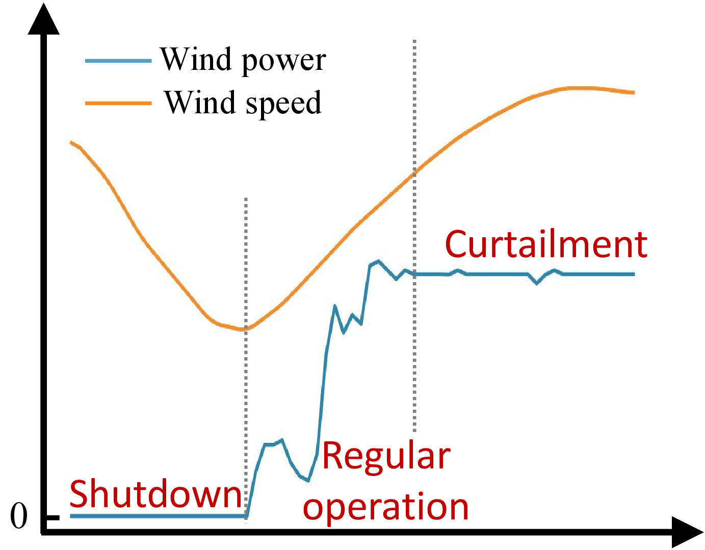
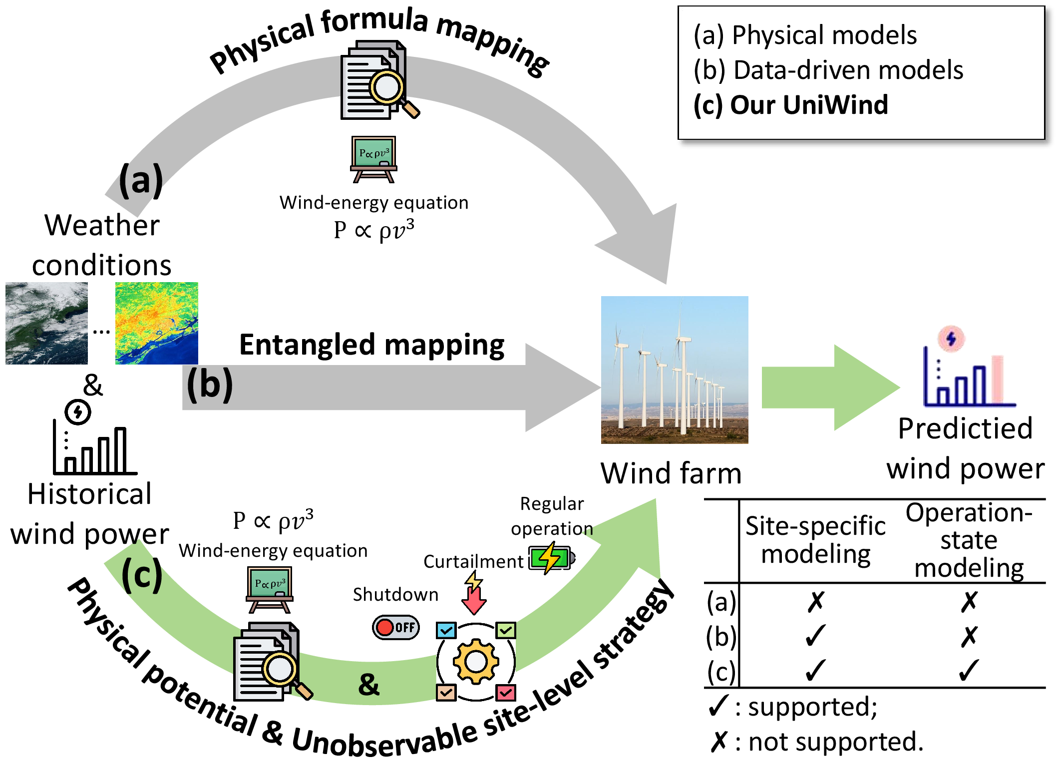
Existing wind power forecasting methods can be categorized into physically driven and data-driven approaches. Physical models [9]–[11], detailed in Figure 1 (a), provide reliable power predictions through physical constraints and structured inductive biases. However, they struggle to capture local endogenous factors, such as terrain-induced circulation and wind-farm operational states. As shown in Figure 2, turbines may switch among shutdown with zero output, regular operation where power follows the physical wind-speed response, and curtailment where output is intentionally constrained below the available power potential. These latent-state changes alter the wind-to-power mapping, limiting the adaptability of fixed physical formulations across different wind farms and operational conditions. Data-driven methods [12]–[16] can capture richer correlations from real-world data. Nevertheless, as shown in Figure 1 (b), they tend to entangle physical power potential with hidden-state effects, making it difficult to determine whether power deviations arise from meteorological changes or latent operational states. This weakens their robustness under diverse wind and operational conditions. Therefore, robust day-ahead wind power forecasting requires explicitly modeling the dependency from meteorological conditions to physical power potential and further to realized power under hidden-state interventions, as illustrated in Figure 1 (c). However, constructing such a robust model poses two key challenges:
First, estimating power generation potential requires balancing universal physical principles with site-specific adaptation. Wind power generation follows physical relationships that provide reusable structure across wind farms. However, real-world generation potential is also shaped by site-specific factors, such as local environmental effects, that are often unobserved. Existing fixed physical formulas [11], [17] may be too rigid to capture site-dependent wind-to-power responses, whereas unconstrained data-driven methods [18], [19] may overfit noisy site-specific correlations or violate physical principles. Therefore, an effective physical prior should preserve wind-energy physics while enabling site-level calibration under appropriate constraints.
Second, predicting realized power requires modeling the effects of unobservable, time-varying future operational states. Even when the physical generation potential is similar, the actual output may differ due to different latent states like shutdown or curtailment. These dynamic states are often unobservable at forecasting time and are entangled with meteorological variation. Meanwhile, existing hidden-state-aware methods [20], [21] typically infer hidden states directly from historical sequences, making it difficult to distinguish true changes in physically available power from hidden-state interventions. As a result, they may average over multiple states and fail to capture abrupt transitions or abnormal dynamics. This motivates the inference of future states and the design of state-specific dependency correction.
To this end, we propose UniWind, a physics-informed state-routing model for day-ahead wind power forecasting. UniWind decouples physically available power from operationally induced deviations, thereby modeling both meteorology-driven generation potential and its state-dependent realization. To address the first challenge, UniWind introduces a Physical Prior Estimator that combines site-conditioned monotone warping and a shared physical power curve to construct a site-calibrated physical prior. As the physical prior represents the ideal generation potential under given meteorological conditions, we treat it as an upper bound on realized power and construct an upper-bound constraint accordingly. To address the second challenge, UniWind uses a Latent State Encoder to infer historical operating patterns from prior-power discrepancies and retrieve future state embeddings from similar meteorological contexts. Since future operational states are dynamic and require distinct correction mechanisms, a State-aware Power Corrector then routes each timestamp to supervised operating-state experts and applies bounded state-specific corrections to obtain realized power forecasts. Our contributions are summarized as follows:
We propose UniWind, a physics-informed state-routing model for day-ahead wind power forecasting that explicitly factorizes the forecasting process into meteorology-driven physical power potential and state-dependent realized generation.
We develop a site-calibrated Physical Prior Estimator that learns an available-power prior by combining shared wind-energy structure with site-conditioned monotone calibration and physical upper-bound regularization.
We introduce a Latent State Encoder and a State-aware Power Corrector to model unobservable operational states and their effects on wind-farm generation. The encoder retrieves future state representations from historical weather-state patterns, while the corrector uses knowledge-supervised state routing and bounded state-specific experts to transform the physical prior into realized power forecasts.
We conduct extensive experiments on more than 20 real-world wind-farm datasets that cover full-shot and cross-farm zero-shot settings, and demonstrate the accuracy and robustness of UniWind.
2 Related Work↩︎
Wind Power Forecasting. Current research on wind power forecasting primarily relies on physical models or data-driven approaches. Physical models [9]–[11] estimate wind power by propagating meteorological forecasts through physical and engineering assumptions. For example, Li et al. [10] first simulate steady-state flow fields under discrete inflow wind conditions to construct a database, and then predict short-term wind power by querying this database using wind inputs. Data-driven models learn mappings from meteorological variables, historical power, and site features to future generation. Statistical methods [12], [13], [18], [22], [23] typically rely on handcrafted feature engineering. Tree-based approaches, such as XGBoost [22] and LightGBM [23], combine diverse meteorological features, and often serve as strong practical baselines. Deep learning models [14]–[16], [24], [25] learn nonlinear weather-power dependencies from large-scale observations. More recently, following the emergence of foundation-model research [26], [27], WindFM [28] has been developed for wind energy prediction in unseen scenarios. Although these methods capture rich empirical correlations, real-world wind-farm data often contain measurement noise, local environmental effects, and latent operational states, such as shutdowns and curtailment. Consequently, physical models may fail to adapt to local endogenous conditions, whereas data-driven models may absorb hidden operational effects as noise or spurious correlations. Neither line of work explicitly separates physical generation potential from state-dependent realized power, which is the key gap addressed by UniWind.
Solar Power Forecasting. Solar power forecasting models use weather conditions and historical observations, but rely more on cloud-sensitive multimodal signals [29]–[32]. For example, CrossViViT [29] uses satellite imagery as spatio-temporal context and combines it with station time series for probabilistic forecasting. FusionSF [30] discretizes heterogeneous modalities into a shared codebook for robust solar-power generation. However, wind power depends mainly on wind-speed dynamics rather than irradiance, and its uncertainty is more affected by turbine operation than cloud motion. These differences limit the direct transfer of solar forecasting models to wind power prediction.
Time-Series Forecasting for Wind Power. Time-series forecasting is widely used for wind power prediction because it directly learns temporal dependencies from historical sequences [3], [6], [33]. Recent models such as PatchTST [7], iTransformer [5], and xPatch [4] improve long-horizon forecasting through patch-based, variable-centric, and multi-period representations. Foundation models such as Chronos [34] and Moirai [35] leverage large-scale heterogeneous time-series pretraining for downstream adaptation. Nonetheless, these generic sequence forecasting models are often dominated by historical power patterns and may inadequately capture how future meteorological changes drive wind generation.
3 Methodology↩︎
In this section, we present UniWind, a unified wind power forecasting model that combines physics-informed priors with latent operational state dynamics.
3.1 Problem Statement↩︎
Given the numerical weather prediction (NWP) sequence \(\boldsymbol{w}\in\mathbb{R}^{(T_1+T_2) \times N_w}\), the historical power sequence \(\boldsymbol{x}\in \mathbb{R}^{T_1}\), and the site features \(\boldsymbol{c}\in\mathbb{R}^{N_s}\) of the target wind farm, our goal is to learn a forecasting model \(f_\theta\) that predicts wind power \(\hat{\boldsymbol{y}}\in\mathbb{R}^{T_2}\): \[\hat{\boldsymbol{y}} = f_\theta\left( \boldsymbol{w}, \boldsymbol{x}, \boldsymbol{c} \right),\] where \(T_1\) and \(T_2\) denote the lengths of the historical and forecasting horizons, respectively. \(N_w\) is the number of meteorological features, and \(N_s\) is the number of static site features, such as longitude, latitude, and rated power.

3.2 Overall Framework↩︎
As shown in Figure 3, UniWind consists of three stages. First, the Physical Prior Estimator combines density-aware wind-speed normalization, site-conditioned physical calibration, and a shared learnable power curve to estimate the physical prior under ideal conditions. A physical upper-bound constraint further encourages this prior to serve as a soft envelope for available generation. Second, the Latent State Encoder characterizes historical operational states using discrepancies between observed power and the physical prior. It then retrieves future state patterns from historical states under similar meteorological conditions, refines the operational-state embeddings, and fuses them with weather embeddings to obtain the final state embeddings. Finally, the State-aware Power Corrector routes the final state embedding at each time step to supervised operational-state experts and aggregates bounded, state-specific corrections to produce the final prediction.
3.3 Physical Prior Estimator↩︎
Given that wind power is governed by strong site-specific physical constraints, we propose a Physical Prior Estimator to construct site-calibrated estimates of physically available power, providing a reliable prior for latent state modeling and state-aware correction.
Physical normalization. To remove first-order variations in air density, we apply a density-aware wind-speed adjustment [36] to obtain the equivalent wind speed \(\tilde{\boldsymbol{v}} = \boldsymbol{v} \left(\frac{\boldsymbol{\rho}}{\rho_0}\right)^{1/3}\), which follows the wind-energy relation \(P_{\mathrm{wind}}\propto \rho v^3\). Here, \(\boldsymbol{v} \in \mathbb{R}^{T_1+T_2}\) and \(\boldsymbol{\rho}\in \mathbb{R}^{T_1+T_2}\) denote the raw wind speed and air density over the past \(T_1\) and future \(T_2\) timestamps, respectively, and \(\rho_0=1.225\) denotes the reference air density.
Site-conditioned monotone warp. To adapt the physical prior to different sites while remaining sufficiently constrained to avoid non-physical wind-speed inversions, we design a site-conditioned monotone warp that maps equivalent wind speed to effective wind speed as follows: \[\hat{\boldsymbol{v}} = \max\left(0,\; \exp(a)(1+\tilde{\boldsymbol{v}})^{\exp(b)} - 1\right), \qquad [a,b]^\top = h_{\phi}(\boldsymbol{c}) \in \mathbb{R}^{2}.\] Here, \(\boldsymbol{c}\in\mathbb{R}^{N_s}\) denotes the site features, \(h_{\phi}(\cdot)\) is an MLP-based site-conditioned parameter head, \(a\) shifts the effective speed scale, and \(b\) controls the local stretch of the curve. The mapping from \(\tilde{\boldsymbol{v}}\) to \(\hat{\boldsymbol{v}}\) preserves the ordering of wind speeds, so a larger equivalent wind speed cannot yield a smaller effective wind speed. A formal proof is provided in Appendix 8.1.
To further align the shared power curve with the target wind farm, UniWind learns site-conditioned anchors \([v_b,v_r]^\top \in \mathbb{R}^{2}\), with \(v_r>v_b\), in the same manner as \(a\) and \(b\). Here, \(v_b\) and \(v_r\) denote cut-in-like and rated-speed-like anchors. We then normalize the effective wind speed as \(\boldsymbol{v}^* = \frac{ \hat{\boldsymbol{v}}-v_b }{ v_r-v_b }\).
Shared physical power curve. After site-conditioned wind-speed calibration, we introduce a shared physical power curve as a smooth, learnable physical prior inspired by classical wind-turbine power curves [37]. Rather than reproducing a specific manufacturer curve, this curve captures the common physical structure of wind generation: near-zero power before cut-in, nonlinear growth in the sub-rated region, and saturation near rated capacity. The physical prior power is generated as follows: \[\boldsymbol{p}^{\mathrm{prior}} = P_{\mathrm{cap}} f_{\mathrm{curve}}(\boldsymbol{v}^*),\] where \(P_{\mathrm{cap}}\in \mathbb{R}\) denotes the rated capacity of the target wind farm, and \(f_{\mathrm{curve}}(\cdot)\) maps the normalized effective wind speed \(\boldsymbol{v}^*\) to a capacity factor in \([0,1]\). The detailed parameterization of \(f_{\mathrm{curve}}\) is provided in Appendix 8.2.
Physical upper-bound constraint. We further shape the physical prior into a soft upper envelope of available generation. The prior should be high enough to cover observed power, while remaining close to real power under regular operation. We therefore define \[\mathcal{L}_{\mathrm{prior}} = \frac{1}{|\Omega|} \sum_{t\in\Omega} \left[ \boldsymbol{p}_t-\boldsymbol{p}_t^{\mathrm{prior}} \right]_+ + \lambda_{\mathrm{tight}} \frac{1}{|\Omega_{\mathrm{reg}}|} \sum_{t\in\Omega_{\mathrm{reg}}} \left[ \boldsymbol{p}_t^{\mathrm{prior}} - \boldsymbol{p}_t - \epsilon_{\mathrm{slack}} \right]_+ .\] Here, \(\Omega\) and \(\Omega_{\mathrm{reg}}\) denote the set of observed time steps and the subset labeled as regular state, respectively. The construction of the regular label is detailed in Appendix 8.3. We define \([x]_+=\max(x,0)\), and \(\epsilon_{\mathrm{slack}}\) is the allowed slack between the physical prior and observed power. The weight \(\lambda_{\mathrm{tight}}\) controls the regular-state tightness.
3.4 Latent State Encoder↩︎
By encoding historical deviations and retrieving future state patterns from weather context, this module produces state embeddings that explain the gap between ideal physical availability and actual wind-farm generation.
Historical state encoding. We use historical discrepancies between observed power and theoretically available power to infer recent latent operating behavior. Let \(1{:}T_1\) denote the historical window and \(T_1{+}1{:}T_1+T_2\) denote the future window. Given the historical real power \(\boldsymbol{x}\) and the historical physical prior \(\boldsymbol{p}^{\mathrm{prior}}_{1:T_1}\), UniWind constructs discrepancy-aware historical state tokens: \[\boldsymbol{\psi} = \left[ \boldsymbol{x},\; \boldsymbol{p}^{\mathrm{prior}}_{1:T_1},\; \boldsymbol{e},\; \Delta \boldsymbol{x},\; \Delta \boldsymbol{p}^{\mathrm{prior}}_{1:T_1},\; \Delta \boldsymbol{e},\; \boldsymbol{r},\; \Delta \boldsymbol{r} \right].\] Here, \(\boldsymbol{\psi}\in\mathbb{R}^{T_1\times 8}\) denotes the historical state-token sequence, \(\boldsymbol{e}=\boldsymbol{x}-\boldsymbol{p}^{\mathrm{prior}}_{1:T_1}\) denotes the residual sequence, \(\boldsymbol{r}\) denotes the power-to-prior ratio sequence, and \(\Delta\) denotes the first-order temporal difference operator. These tokens are then encoded into \(D\)-dimensional historical state embeddings: \[\boldsymbol{s}^h = E_{\mathrm{hist}}(\boldsymbol{\psi}).\] Here, \(E_{\mathrm{hist}}(\cdot)\) denotes the historical state encoder, which consists of token normalization, an MLP projection, and a multi-scale temporal convolution block, and \(\boldsymbol{s}^h\in\mathbb{R}^{T_1\times D}\) denotes the historical state embedding sequence.
Weather encoding. UniWind encodes the full weather sequence as follows: \[\tilde{\boldsymbol{h}}^w = E_{\mathrm{w}}(\boldsymbol{w}), \qquad \boldsymbol{h}^w = T_{\mathrm{w}}(\tilde{\boldsymbol{h}}^w).\] Here, \(\boldsymbol{w}\in\mathbb{R}^{(T_1+T_2)\times N_w}\) is the NWP sequence, \(E_{\mathrm{w}}(\cdot)\) is an MLP-based per-step weather encoder, \(T_{\mathrm{w}}(\cdot)\) is a temporal weather encoder with positional and time information, and \(\boldsymbol{h}^w\in\mathbb{R}^{(T_1+T_2)\times D}\) is the context-aware weather embedding sequence.
Future latent state retrieving. To transfer operating-state patterns from similar historical meteorological conditions to future horizons, we treat future weather embeddings as queries, historical weather embeddings as keys, and historical state embeddings as values, thereby retrieving future latent state embeddings as follows: \[\tilde{\boldsymbol{s}}^f = \operatorname{Attn} \left( Q\boldsymbol{h}^w_{T_1+1:T_1+T_2},\; K\boldsymbol{h}^w_{1:T_1},\; V\boldsymbol{s}^h_{1:T_1} \right).\] Here, \(\tilde{\boldsymbol{s}}^f\in\mathbb{R}^{T_2\times D}\) denotes the retrieved future state sequence, and \(Q\), \(K\), and \(V\) denote learnable query, key, and value projections, respectively.
Latent state refining. Future operational states are correlated with past operational states and influenced by future weather conditions. Therefore, UniWind refines the full state sequence \([\boldsymbol{s}^h;\tilde{\boldsymbol{s}}^f]\) using a causal TCN-based refiner. It then fuses the refined state features with weather features through projection and an MLP to obtain the final state embedding sequence \(\boldsymbol{z}\in\mathbb{R}^{(T_1+T_2)\times D}\).
3.5 State-aware Power Corrector↩︎
To convert ideal available power into realistic forecasts under hidden operating conditions, we propose the State-aware Power Corrector, which learns state-dependent corrections to the physical prior using the inferred state embeddings.
Site-context conditioning. The same latent operating pattern may require different corrections across wind farms. To incorporate such persistent site information, UniWind encodes site context and injects it into the final state embeddings: \[\boldsymbol{c}^{\mathrm{ctx}} = E_{\mathrm{ctx}}(\boldsymbol{c}, \boldsymbol{x}), \qquad \tilde{\boldsymbol{z}} = \operatorname{LN}(\boldsymbol{z} + \boldsymbol{c}^{\mathrm{ctx}}).\] Here, \(E_{\mathrm{ctx}}(\cdot)\) is an MLP-based site-context encoder that fuses site features and historical power statistics, \(\boldsymbol{c}^{\mathrm{ctx}}\in\mathbb{R}^{D}\) is the correction-side site embedding, \(\tilde{\boldsymbol{z}}\in\mathbb{R}^{(T_1+T_2)\times D}\) is the site-aware latent state sequence, and \(\operatorname{LN}(\cdot)\) denotes layer normalization.
Supervised state routing. Different operational states require distinct correction strategies. Accordingly, UniWind routes each state embedding to state-specific experts and supervises the routing process with state-prior labels: \[\hat{\boldsymbol{l}} = \operatorname{softmax}(R(\tilde{\boldsymbol{z}})), \qquad \mathcal{L}_{\mathrm{router}} = \operatorname{CE}(\hat{\boldsymbol{l}}, \boldsymbol{l}).\] Here, \(R(\cdot)\) is an MLP-based state router, \(\hat{\boldsymbol{l}}\in\mathbb{R}^{(T_1+T_2)\times 3}\) contains the probabilities of three operating-state experts: regular, curtailment and shutdown. \(\operatorname{CE}(\cdot,\cdot)\) denotes the cross-entropy loss. The state-prior labels for the historical and future windows, denoted by \(\boldsymbol{l}\), are derived from wind-power behavior rather than ground-truth operational annotations. Their construction is detailed in Appendix 8.3.
State-specific correction. To make the correction features both state-specific and temporally contextualized, UniWind first transforms the site-aware latent sequence \(\tilde{\boldsymbol{z}}\) with expert-specific MLPs. The resulting expert-conditioned features are weighted by the routing probabilities and then refined by a shared self-attention layer, producing an interaction-aware correction embedding \(\boldsymbol{z}'\in\mathbb{R}^{(T_1+T_2)\times D}\). Based on this embedding, UniWind assigns expert-specific scaling and upper-bound parameters: \[\begin{align} (\boldsymbol{\alpha}^{\mathrm{sd}}, \boldsymbol{\beta}^{\mathrm{sd}}) = (\boldsymbol{0}, \boldsymbol{0}), \qquad (\boldsymbol{\alpha}^{\mathrm{cur}}, \boldsymbol{\beta}^{\mathrm{cur}}) = \left( \boldsymbol{1}, \sigma(H_{\beta}(\boldsymbol{z}')) \right), \qquad (\boldsymbol{\alpha}^{\mathrm{reg}}, \boldsymbol{\beta}^{\mathrm{reg}}) = \left( \sigma(H_{\alpha}(\boldsymbol{z}')), \boldsymbol{1} \right), \end{align}\] where \(H_{\alpha}(\cdot)\) and \(H_{\beta}(\cdot)\) denote MLP-based parameter heads. The shutdown expert \(\mathrm{sd}\) sets both the scaling factor and upper bound to zero, the curtailment expert \(\mathrm{cur}\) learns an upper bound ratio, and the regular expert \(\mathrm{reg}\) learns a multiplicative correction under the rated-capacity bound.
For each expert \(e\in\{\mathrm{sd},\mathrm{reg},\mathrm{cur}\}\), the bounded expert output is computed as follows: \[\hat{\boldsymbol{p}}^{e} = \operatorname{clip} \left( \boldsymbol{\alpha}^{e}\odot\boldsymbol{p}^{\mathrm{prior}}, 0, \boldsymbol{\beta}^{e}P_{\mathrm{cap}} \right).\] The final forecast is the routing-weighted aggregation of expert outputs: \[\hat{\boldsymbol{p}} = \sum_{e\in\{\mathrm{sd},\mathrm{reg},\mathrm{cur}\}} \hat{\boldsymbol{l}}_{e}\odot \hat{\boldsymbol{p}}^{e},\] where \(\hat{\boldsymbol{p}}\in\mathbb{R}^{T_1+T_2}\) is the predicted power sequence and \(\hat{\boldsymbol{l}}_{e}\) denotes the routing probability for expert \(e\). For clarity, we denote the historical segment \(\hat{\boldsymbol{p}}_{1:T_1}\) as \(\hat{\boldsymbol{x}}\) and the future segment \(\hat{\boldsymbol{p}}_{T_1+1:T_1+T_2}\) as \(\hat{\boldsymbol{y}}\).
3.6 Training Objectives↩︎
Because historical reconstruction stabilizes the learned operational states, and future prediction directly optimizes the forecasting target, we construct the mean squared error loss as follows: \[\mathcal{L}_{\mathrm{mse}} = \left\lVert \hat{\boldsymbol{x}}-\boldsymbol{x}\right\rVert_F^2 + \left\lVert \hat{\boldsymbol{y}}-\boldsymbol{y}\right\rVert_F^2,\] where \(\boldsymbol{x}\) and \(\boldsymbol{y}\) denote the ground-truth historical and future power sequences, respectively.
The final training objective combines forecasting supervision, physical-prior regularization, and supervised state routing: \[\mathcal{L} = \mathcal{L}_{\mathrm{mse}} + \mathcal{L}_{\mathrm{prior}} + \lambda_{\mathrm{router}}\mathcal{L}_{\mathrm{router}},\] where \(\lambda_{\mathrm{router}}\) is the weight for the router-supervision loss.
4 Experiments↩︎
4.1 Experimental Setup↩︎
Datasets. We evaluate UniWind on 24 real-world datasets collected from distinct wind farms. These datasets include the Penmanshiel [38] and Kelmarsh [39] wind farms in the UK, while the remaining datasets span three provinces in China: Shandong, Shanxi, and Anhui. The corresponding NWP data are obtained from the European Centre for Medium-Range Weather Forecasts (ECMWF)1 and the Global Forecast System (GFS)2. All datasets are uniformly processed at 15-minute intervals. Detailed summaries of the datasets are provided in Appendix Tables 2 and 3. For each dataset, we use the last two months for testing, the preceding two month for validation, and earlier data for training, removing overlapping windows at split boundaries.
Baselines. We compare UniWind with representative and state-of-the-art models for day-ahead wind power forecasting, which are categorized into five groups: Physical models. We include PowerCurve [40], a physics-based wind-turbine power-curve model that converts meteorological conditions into power estimates using predefined power-curve assumptions. Statistical models. We consider widely used tree-based statistical learning models, including LightGBM [23] and XGBoost [22], which learn nonlinear mappings from meteorological covariates to wind power. Time-series forecasting models. We compare UniWind with competitive long-horizon time-series forecasting models, including PatchTST [7], iTransformer [5], TimeMixer [6], and xPatch [4]. Renewable-energy forecasting models. We further include solar power forecasting models, including CrossViViT [29], FusionSF [30], and the wind power forecasting model 2DXformer [15]. Foundation models. To evaluate zero-shot generalization, we compare UniWind with the wind-specific foundation model WindFM [28] and general time-series foundation models, including Chronos-2 [34] and Moirai [35]. The types of data used by all baselines are reported in Appendix Table 4.
Setup. We evaluate all models using Mean Absolute Error (MAE) and Root Mean Squared Error (RMSE). The historical and future windows, \(T_1\) and \(T_2\), are set to 96 and 192 time steps, respectively, and evaluation is conducted on the last 96 prediction steps. The one-day gap between \(T_2\) and the evaluation window reflects the operational requirement that generation be forecast before the target delivery day. In the full-shot setting, each dataset is trained and evaluated independently using its complete training and test sets. Due to space limitations, we report full-shot results only for SD_A, SX_A, AH_A, and UK_Penmanshiel, with regional average performance provided in Appendix Table 5. In the zero-shot setting, WindFM, Chronos-2, and Moirai are evaluated directly using their officially released checkpoints, while Moirai-PT and UniWind are trained on all datasets except SD_A, SX_A, AH_A, and UK_Penmanshiel, and evaluated separately on these four datasets.
4.2 Experimental Results↩︎
4.2.1 Overall Performance↩︎
Table ¿tbl:tab:baseline? presents the overall performance. We compare the full-shot results of our proposed UniWind with those of end-to-end models, and compare the zero-shot results of our proposed UniWind with those of foundation models. We highlight the best and second-best performance in bold and underline.
llcccccccc * & *Method & & & &
(lr)3-4 (lr)5-6 (lr)7-8 (lr)9-10 * & *& MAE & RMSE & MAE & RMSE & MAE & RMSE & MAE & RMSE
*Full-shot&PowerCurve [40] & 28.64 & 41.79 & 30.04 & 37.42 & 54.96 & 64.76 & 6.02
& 7.42
&LightGBM [23] & 14.90 & 23.91 & 11.56 & 15.89 & 27.58 & 35.51 & 3.70 &
4.57
&XGBoost [22] & 15.10 & 24.25 & 15.42 & 18.61 & 26.21 & 33.84 & 4.00 & 4.77
*&patchTST [7] & 31.75 & 46.57 & 19.91 & 32.04 & 41.61 & 54.40 & 4.49 & 5.77
*&iTransformer [5] & 35.64 & 47.50 & 19.25 & 31.14 & 44.40 & 57.38 & 5.54 & 7.03
*&TimeMixer [6] & 34.50 & 46.82 & 19.64 & 29.94 & 42.92 & 53.97 & 4.90 & 5.93
*&xPatch [4] & 33.42 & 44.86 & 19.71 & 32.04 & 45.53 & 58.51 & 5.42 & 6.84
*&CrossViViT [29] & 31.80 & 40.29 & 25.31 & 29.38 & 36.62 & 45.44 & 5.02 & 5.99
*&FusionSF [30] & 25.64 & 36.41 & 14.20 & 22.63 & 17.12 & 22.72 & 4.52 & 5.87
*&2DXformer [15] & 25.37 & 35.33 & 12.40 & 17.76 & 23.58 & 32.09 & 4.31 & 5.75
*&UniWind & 12.05 & 18.05 & 10.20 & 15.41 & 12.66 & 17.92 & 3.51 &
4.53
*&Improvement (%) & 19.13 & 24.51 & 11.76 & 3.02 & 26.05 & 21.13 & 5.14 & 0.88
*Zero-shot&WindFM [28] & 29.40 & 43.37 & 28.49 & 36.81 & 38.04 & 50.23 & 5.17
& 6.44
*&Chronos-2 [34] & 34.39 & 51.45 & 19.00 & 31.97 & 49.30 & 64.17 & 6.62 & 8.66
*&Moirai [35] & 39.03 & 52.08 & 19.95 & 30.52 & 52.71 & 63.32 & 5.35 & 6.86
*&Moirai-PT [35] & 32.05 & 45.06 & 17.39 & 27.18 & 38.63 & 49.83 & 4.15 &
5.24
*&UniWind & 14.56 & 21.79 & 12.30 & 18.61 & 14.28 & 18.17 & 3.87 &
5.12
*&Improvement (%) & 50.48 & 49.76 & 29.27 & 31.53 & 62.46 & 63.54 & 6.75 & 2.29
Full-shot prediction. As shown in Table ¿tbl:tab:baseline?, UniWind achieves the best full-shot performance across all representative datasets and evaluation metrics. Similar trends are observed in the regional average results reported in Appendix Table 5. Among the baselines, the physics-only PowerCurve performs poorly, suggesting that fixed power-curve assumptions cannot adequately capture site-specific environmental effects or latent operational states in real-world wind farms. Statistical models, LightGBM and XGBoost, remain strong practical baselines on several datasets, but their performance is less stable across regions because they primarily learn empirical weather-power correlations. Time-series forecasting models that rely on historical sequence patterns generally underperform, confirming that historical power and NWP data are insufficient for day-ahead wind power forecasting. Renewable-energy forecasting models, including CrossViViT, FusionSF, and 2DXformer, further incorporate future NWP information and therefore provide richer meteorological context. FusionSF is particularly competitive on AH_A. However, these models still lag behind UniWind across all reported metrics, as they do not fully disentangle physically available power from latent operational effects. By combining a site-calibrated physical prior with state-aware correction, UniWind better preserves transferable wind-power structure while adapting to sample-specific operational states.
Zero-shot prediction. Table ¿tbl:tab:baseline? reports zero-shot results against wind-specific and general time-series foundation models. UniWind substantially outperforms WindFM, Chronos-2, Moirai, and Moirai-PT across all datasets and metrics. Among the baselines, WindFM performs best on SD_A, whereas Moirai-PT performs best on SX_A and UK_Penmanshiel. However, all foundation-model baselines lag behind UniWind, indicating that wind-domain pretraining or generic time-series pretraining without future NWP and physical priors is insufficient for zero-shot wind power forecasting. These results show that UniWind transfers more effectively across wind farms by combining future NWP covariates with transferable physical prior modeling and state-aware correction.
4.2.2 Performance under Varied Conditions↩︎
Figure 4 evaluates UniWind under different meteorological and operational conditions. We compare UniWind with three representative baselines: XGBoost, PatchTST, and FusionSF.
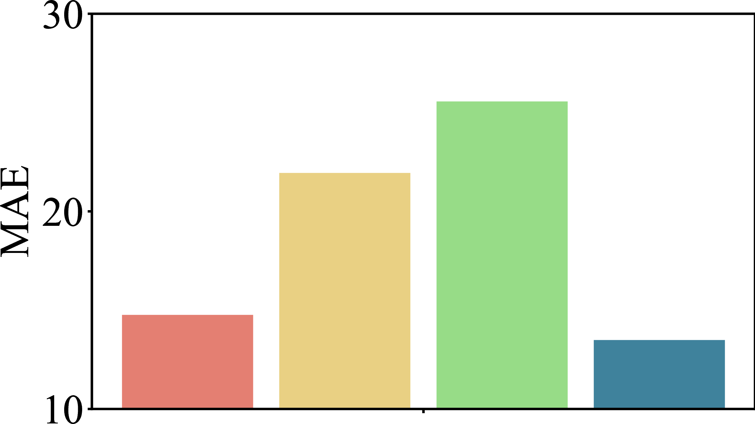
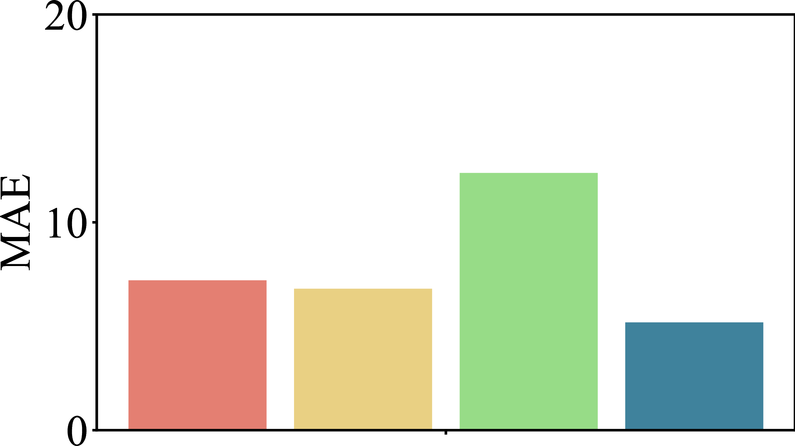

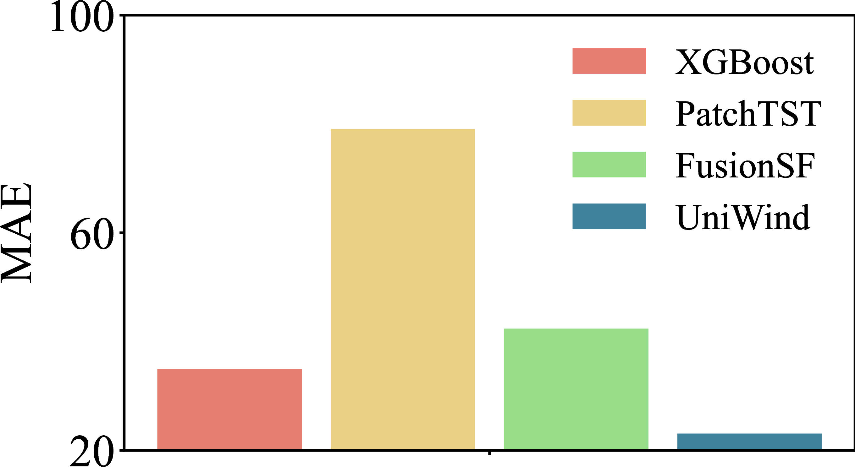
Figure 4: Performance comparison under varied conditions on the SD_A dataset..
We evaluate robustness under joint meteorological and operational conditions by dividing the SD_A test samples into four regimes. Wind speeds below \(9\,\mathrm{m/s}\), corresponding to the 90th percentile on SD_A, are treated as low-wind conditions, whereas the remaining samples are treated as high-wind conditions. Regular and abnormal states are determined using the state-prior labels defined in Appendix 8.3, with shutdown and curtailment grouped as abnormal states. As shown in Figure 4, UniWind achieves the lowest MAE in all four regimes. XGBoost is competitive in regular states, but its advantage diminishes once abnormal operation is introduced. PatchTST performs poorly in most regimes and suffers particularly large errors under high wind speeds. FusionSF degrades when the wind speed is low. In contrast, UniWind remains strong across all regimes and gains most in the high-wind abnormal cases. This supports the core motivation of UniWind: by separating physical power variations induced by wind speed from power deviations induced by operational states, UniWind can follow the physical wind-to-power relationship in regular regimes while correcting deviations in abnormal states.
4.2.3 Ablation Studies↩︎
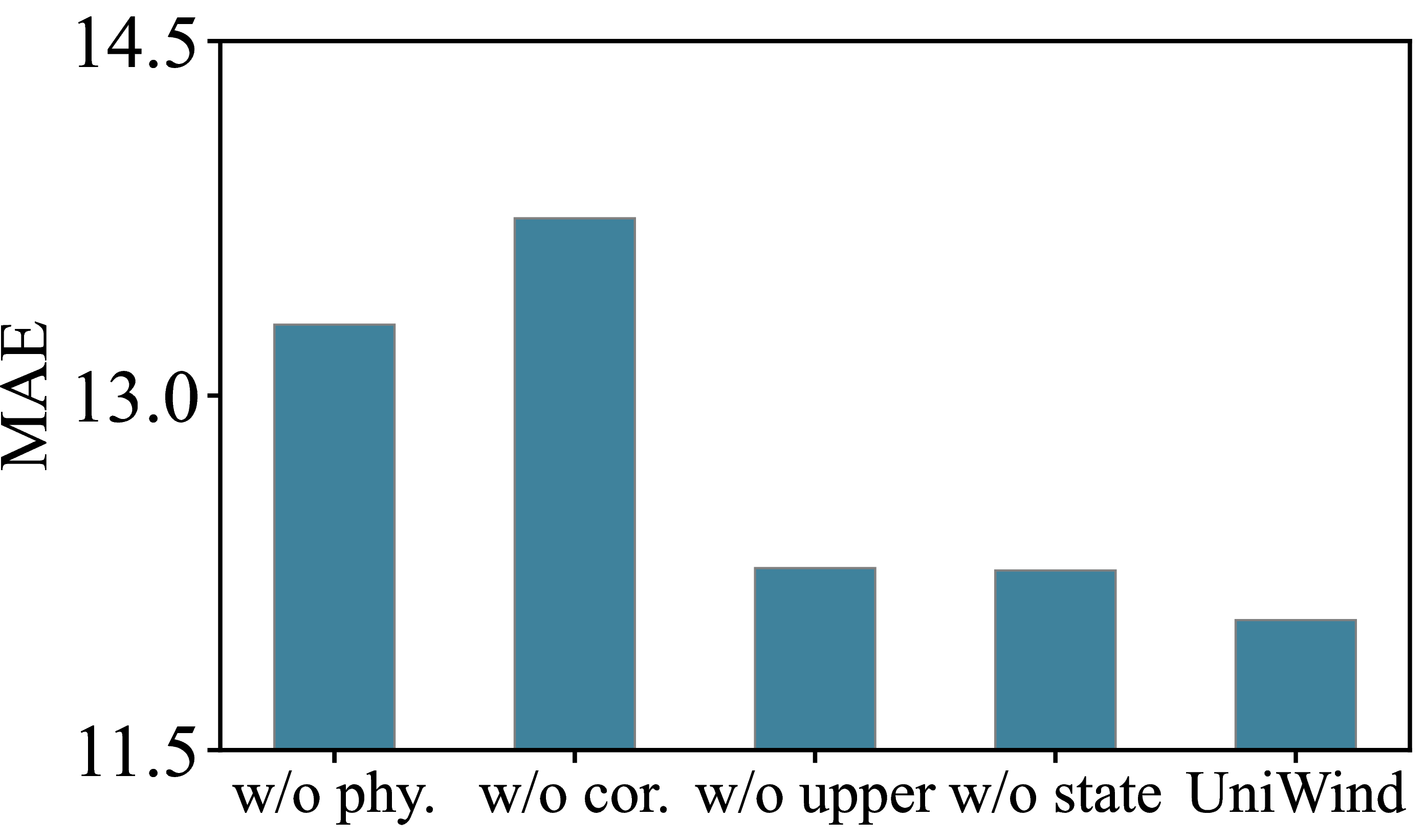
To evaluate the contribution of each component, we construct four variants of UniWind. w/o phy. removes the physical prior and replaces it with a learnable parameter. w/o cor. directly uses the physical prior as the final prediction. w/o upper removes the physical upper-bound constraint from the Physical Prior Estimator. w/o state removes the supervised state routing loss \(\mathcal{L}_{router}\).
As shown in Figure 5, all variants perform worse than the full UniWind, demonstrating that each component contributes to the forecasting accuracy. The largest degradation appears in w/o cor., indicating that directly using the physical prior is insufficient because realized wind power is strongly affected by latent operational states. w/o phy. also shows a clear performance drop, confirming that the physical prior provides an important available-power reference for subsequent correction. Removing the upper-bound constraint or the state classification loss leads to smaller but still noticeable degradation, suggesting that physical regularization and knowledge-guided state supervision further stabilize the learned prior and improve state-aware correction.
| SD_A | WindFM | Chronos-2 | Moirai | UniWind |
|---|---|---|---|---|
| Parameters (M) | 1.6 | 119.5 | 11.4 | 4.0 |
| Inference time (ms/sample) | 0.56 | 25.06 | 26.35 | 0.72 |
r0.56
0.5mm
4.2.4 Efficiency Comparison↩︎
Table 1 compares the computational efficiency of UniWind with representative foundation-model baselines on the SD_A dataset. UniWind has only 4.0M parameters, far fewer than Chronos-2 and Moirai, while remaining moderately larger than WindFM. In terms of inference efficiency, UniWind requires 0.72 ms per sample, achieving a speed comparable to WindFM and substantially faster than Chronos-2 and Moirai. These results show that UniWind improves forecasting accuracy without relying on large foundation-model scale, making it efficient for repeated day-ahead forecasting across wind farms.
5 Conclusion, Limitations, and Future Work↩︎
In this paper, we propose UniWind, a day-ahead wind power forecasting model that captures the structured dependency from meteorological conditions to physically available power and realized generation under latent operational states. UniWind first constructs a site-calibrated physical prior through site-conditioned monotone warping, a shared physical power curve, and a physical upper-bound constraint. It then uses a State-aware Power Corrector to transform this available-power prior into final forecasts through knowledge-guided state routing and bounded state-specific correction. Extensive experiments on more than 20 real-world wind-farm datasets demonstrate that UniWind achieves strong full-shot and zero-shot performance and remains effective across diverse operating conditions. We believe that UniWind can promote the safe, economical, and efficient integration of wind power into future low-carbon energy systems.
Like other NWP-driven day-ahead forecasting methods, UniWind still relies on the quality of NWP inputs. However, the proposed site-calibrated physical prior and state-aware correction help mitigate this dependence. Future work will explore the integration of additional meteorological observations to better capture local weather dynamics and further improve forecasting reliability.
6 Datasets↩︎
We provide detailed information on the datasets used in this study. The wind power data were collected from 24 wind farms across four geographically distinct regions: Anhui, Shandong, and Shanxi in China, and the United Kingdom. Table 2 summarizes the basic information of these wind power datasets, including their temporal coverage, temporal interval, and installed capacity. Table 3 reports the numerical weather prediction (NWP) datasets used as meteorological covariates. Since GFS data are unavailable for the UK datasets, only ECMWF data are used for this region. In addition, only five ECMWF features are available for the UK datasets: temperature2m, surfacePressure, windSpeed100m, windDirection100m, and airDensity. Accordingly, we use only these five features for training and evaluation on the UK datasets and adopt the same feature set in the zero-shot experiments to ensure input consistency.
The raw data sources have different temporal resolutions. During preprocessing, we resample the wind power and NWP sequences by upsampling or downsampling as needed and align all variables to a unified 15-minute interval. We match each wind farm with the corresponding NWP grid point based on its latitude and longitude. For wind-farm datasets using two meteorological sources, we concatenate the feature dimensions from both sources as the weather sequence. To avoid information leakage among the training, validation, and test sets, we remove overlapping sequences around the split boundaries. All reported prediction results are computed after the model outputs are denormalized.
| Dataset | Province | Temporal Duration | Temporal Interval | Capacity (MW) |
|---|---|---|---|---|
| AH_A | Anhui, China | 20230101-20241031 | 15 minutes | 149 |
| AH_B | Anhui, China | 20230101-20241031 | 15 minutes | 49.5 |
| AH_C | Anhui, China | 20230101-20241031 | 15 minutes | 49.5 |
| AH_D | Anhui, China | 20230101-20241031 | 15 minutes | 50 |
| AH_E | Anhui, China | 20230101-20241031 | 15 minutes | 64 |
| AH_F | Anhui, China | 20230101-20241031 | 15 minutes | 98 |
| AH_G | Anhui, China | 20230101-20241031 | 15 minutes | 100 |
| AH_H | Anhui, China | 20230101-20241031 | 15 minutes | 50 |
| SD_A | Shandong, China | 20240522-20251110 | 15 minutes | 147.75 |
| SD_B | Shandong, China | 20240522-20251110 | 15 minutes | 99 |
| SD_C | Shandong, China | 20240522-20251110 | 15 minutes | 250 |
| SD_D | Shandong, China | 20240522-20251110 | 15 minutes | 603.5 |
| SD_E | Shandong, China | 20240522-20251110 | 15 minutes | 198 |
| SD_F | Shandong, China | 20240522-20251110 | 15 minutes | 154 |
| SD_G | Shandong, China | 20240522-20251110 | 15 minutes | 99.5 |
| SX_A | Shanxi, China | 20241202-20251214 | 15 minutes | 95 |
| SX_B | Shanxi, China | 20241202-20251214 | 15 minutes | 122 |
| SX_C | Shanxi, China | 20241202-20251214 | 15 minutes | 47 |
| SX_D | Shanxi, China | 20241202-20251214 | 15 minutes | 137 |
| SX_E | Shanxi, China | 20241202-20251214 | 15 minutes | 20 |
| SX_F | Shanxi, China | 20241202-20251214 | 15 minutes | 24 |
| SX_G | Shanxi, China | 20241202-20251214 | 15 minutes | 11 |
| Kelmarsh | Northamptonshire, England | 20170925-20210228 | 10 minutes | 12.3 |
| Penmanshiel | Scottish Borders, England | 20170925-20210228 | 10 minutes | 16.4 |
| Dataset | Temporal Interval | Features |
|---|---|---|
| ECMWF | One hour | Temperature2m, relativeHumidity2m, windSpeed10m, windDirection10m, windSpeed100m, windDirection100m, pressure_msl, surfacePressure, airDensity |
| GFS | One hour | Temperature2m, relativeHumidity2m, windSpeed10m, windDirection10m, windSpeed80m, windDirection80m, windSpeed120m, windDirection120m, pressure_msl, surfacePressure, airDensity |
7 Experimental Details↩︎
7.1 Implementation Details↩︎
UniWind is implemented in PyTorch, and all experiments are conducted on an NVIDIA GeForce RTX 2080 Ti 11 GB GPU. All baselines follow their original designs and use the parameter settings reported in their respective papers. For UniWind, we use Adam with an initial learning rate of \(1 \times 10^{-4}\), a weight decay of \(1 \times 10^{-5}\), and a ReduceLROnPlateau scheduler with a decay factor of 0.5 and a patience of 5. \(\epsilon_{\mathrm{slack}}\), \(\lambda_{\mathrm{tight}}\), and \(\lambda_{\mathrm{router}}\) are set to 1, 0.01, and 0.4, respectively. The hidden dimension \(D\) is 256. Both the weather encoder and state retriever use 4 attention heads, and the batch size is 32.
7.2 Baselines↩︎
We provide detailed descriptions of the baseline models used in our experiments. These baselines cover physical modeling, statistical learning, time-series forecasting, renewable-energy forecasting, and foundation models.
| Model | Historical NWP | Future NWP | Historical Power |
|---|---|---|---|
| PowerCurve [40] | – | \(\surd\) | – |
| LightGBM [23] | – | \(\surd\) | \(\surd\) |
| XGBoost [22] | – | \(\surd\) | \(\surd\) |
| PatchTST [7] | \(\surd\) | – | \(\surd\) |
| iTransformer [5] | \(\surd\) | – | \(\surd\) |
| TimeMixer [6] | \(\surd\) | – | \(\surd\) |
| xPatch [4] | \(\surd\) | – | \(\surd\) |
| Chronos-2 [34] | – | – | \(\surd\) |
| Moirai [35] | – | – | \(\surd\) |
| Moirai-PT [35] | – | – | \(\surd\) |
| WindFM [28] | \(\surd\) | – | \(\surd\) |
| CrossViViT [29] | \(\surd\) | \(\surd\) | \(\surd\) |
| 2DXformer [15] | \(\surd\) | \(\surd\) | \(\surd\) |
| FusionSF [30] | \(\surd\) | \(\surd\) | \(\surd\) |
PowerCurve [40]: A physics-based wind power model that converts meteorological conditions into power estimates according to predefined wind-turbine power-curve assumptions.
LightGBM [23]: A gradient boosting decision tree model that learns nonlinear mappings from meteorological covariates to wind power generation. It is widely used as a strong statistical baseline for tabular forecasting tasks. We concatenate future NWP and historical power data as input to LightGBM.
XGBoost [22]: An efficient tree-based boosting model that captures nonlinear feature interactions from future NWP variables and provides a strong practical baseline for wind power forecasting. We use future NWP data and historical power data as inputs to XGBoost.
PatchTST [7]: A patch-based Transformer model for long-term time-series forecasting. It segments historical power sequences into patches and models temporal dependencies with a channel-independent design.
iTransformer [5]: A Transformer-based time-series forecasting model that treats variables as tokens and learns multivariate temporal dependencies through an inverted attention structure.
TimeMixer [6]: A time-series forecasting model that mixes temporal patterns across multiple scales, enabling it to capture both short-term and long-term dependencies from historical power observations.
xPatch [4]: A long-horizon forecasting model that enhances patch-based time-series representations for historical sequence modeling.
CrossViViT [29]: A renewable-energy forecasting model originally designed to fuse spatio-temporal weather context with station-level time series. In our experiments, this model is adapted for wind power prediction by incorporating historical and future NWP data as well as historical generation data.
FusionSF [30]: A solar power forecasting model that fuses heterogeneous temporal and weather information. Since satellite cloud imagery is unavailable, we replace the satellite-image branch with historical NWP data.
2DXformer [15]: A wind power forecasting model that captures temporal dependencies from historical weather and power sequences through Transformer-based representation learning. In our experiments, future NWP data are additionally incorporated to ensure consistency across the experimental datasets.
WindFM [28]: A wind power foundation model pretrained on large-scale wind power data. We evaluate it in the zero-shot setting using the released checkpoint.
Chronos-2 [34]: A general-purpose time-series foundation model pretrained on heterogeneous time-series corpora. We evaluate it as a zero-shot forecasting baseline using the released checkpoint.
Moirai [35]: A universal time-series foundation model for zero-shot forecasting across diverse domains. We evaluate it in the zero-shot setting using the released checkpoint.
Moirai-PT [35]: A Moirai variant further pretrained on wind power datasets to assess whether additional wind-domain pretraining improves zero-shot wind power forecasting.
Table 4 summarizes the input information used by each baseline. Here, \(\surd\) indicates that the corresponding input type is used by the model, and “–” indicates that it is not used.
8 Supplementary Methods↩︎
8.1 Supplementary Proof↩︎
Proposition 1 (Monotonicity of the site-conditioned warp). For a given wind farm with site features \(\boldsymbol{c}\), let \([a,b]^\top=h_{\phi}(\boldsymbol{c})\in\mathbb{R}^{2}\), where \(h_{\phi}(\cdot)\) is the site-conditioned parameter head, \(a\) is the site-specific speed-scale parameter, and \(b\) is the site-specific stretch parameter. For any timestamp \(t\), let \(\tilde{v}_t\ge 0\) denote the equivalent wind speed and define the unclipped warp \[g(\tilde{v}_t) = \exp(a)(1+\tilde{v}_t)^{\exp(b)}-1.\] Then \(g(\tilde{v}_t)\) is strictly increasing with respect to \(\tilde{v}_t\). Consequently, the clipped effective wind speed \(\hat{v}_t = \max(0,g(\tilde{v}_t))\) is non-decreasing with respect to \(\tilde{v}_t\).
Proof. For a fixed site, \(a\) and \(b\) are constants with respect to the equivalent wind speed \(\tilde{v}_t\). For \(\tilde{v}_t\ge 0\), the derivative of the unclipped warp is \[\frac{\partial g(\tilde{v}_t)}{\partial \tilde{v}_t} = \exp(a)\exp(b)(1+\tilde{v}_t)^{\exp(b)-1}.\] Since \(\exp(a)>0\), \(\exp(b)>0\), and \(1+\tilde{v}_t>0\), we have \[\frac{\partial g(\tilde{v}_t)}{\partial \tilde{v}_t}>0.\] Therefore, \(g(\tilde{v}_t)\) is strictly increasing on \(\tilde{v}_t\ge 0\).
It remains to consider the clipping operation. The function \(m(x)=\max(0,x)\) is non-decreasing in \(x\). Since \(g(\tilde{v}_t)\) is strictly increasing in \(\tilde{v}_t\), the composition \(m(g(\tilde{v}_t))\) is non-decreasing in \(\tilde{v}_t\). Thus, the clipped effective wind speed \(\hat{v}_t=\max(0,g(\tilde{v}_t))\) preserves wind-speed ordering: a larger equivalent wind speed cannot produce a smaller effective wind speed. The result applies element-wise to the vector form used in the main text. ◻
8.2 Shared Physical Power Curve↩︎
The shared canonical curve \(f_{\mathrm{curve}}(\cdot)\) maps the normalized effective wind speed \(\boldsymbol{v}^*\) to a capacity factor in \([0,1]\), and is inspired by the classical wind-turbine power-curve structure [37]. Specifically, a typical power curve has near-zero output before the cut-in region, nonlinear power growth in the sub-rated region, and a rated-power plateau after the rated-speed region. The nonlinear rising segment is physically motivated by the wind-energy relation \(P_{\mathrm{wind}}\propto \rho v^3\). We do not model the high-wind cut-out regime in this shared available-power curve, because abnormal shutdowns and curtailment effects are handled by the State-aware Power Corrector.
We parameterize this physical prior as an element-wise smooth approximation: \[f_{\mathrm{curve}}(\boldsymbol{v}^*) = \operatorname{clip} \left( g_{\mathrm{on}}(\boldsymbol{v}^*)\,g_{\mathrm{mid}}(\boldsymbol{v}^*)\,h(\boldsymbol{v}^*) + g_{\mathrm{rated}}(\boldsymbol{v}^*),0,1 \right),\] where \(\operatorname{clip}(\cdot,0,1)\) constrains the output to a valid capacity factor. The cut-in gate and rated-region gate are defined as \[g_{\mathrm{on}}(\boldsymbol{v}^*) = \sigma(\tau_{\mathrm{on}}\boldsymbol{v}^*), \qquad g_{\mathrm{rated}}(\boldsymbol{v}^*) = \sigma(\tau_{\mathrm{rated}}(\boldsymbol{v}^*-1)),\] where \(\sigma(\cdot)\) is the sigmoid function, \(\tau_{\mathrm{on}}>0\) controls the sharpness of the cut-in transition, and \(\tau_{\mathrm{rated}}>0\) controls the sharpness of the transition into the rated region. The sub-rated gate and rising segment are \[g_{\mathrm{mid}}(\boldsymbol{v}^*) = 1-g_{\mathrm{rated}}(\boldsymbol{v}^*), \qquad h(\boldsymbol{v}^*) = k\,\mathrm{softplus}(\boldsymbol{v}^*)^{n},\] where \(g_{\mathrm{mid}}(\cdot)\) suppresses the rising segment after the rated region, \(\mathrm{softplus}(x)=\log(1+\exp(x))\) provides a smooth positive basis for the rising segment, \(k>0\) controls the sub-rated scale, and \(n>0\) controls the growth curvature. We use a learnable exponent \(n\) instead of a fixed cubic power because \(P_{\mathrm{wind}}\propto \rho v^3\) describes available wind energy, whereas the effective wind-farm power curve can deviate from an exact cubic law due to turbine efficiency. In implementation, the learnable parameter \(n\) is bounded around the physically motivated cubic regime, while \(k\), \(\tau_{\mathrm{on}}\) and \(\tau_{\mathrm{rated}}\) are constrained to positive ranges. This preserves the primary physical shape of a classical power curve.
8.3 State-Prior Label Construction↩︎
These state-prior labels are weak supervisory signals derived from wind-power behavior rather than ground-truth operational annotations. They provide weak supervision for the state router without requiring manually annotated operational states. For each wind farm, we first construct an empirical available-power curve from wind-power pairs in the training dataset. Let \(\bar v_t\) and \(p_t\) denote the representative wind speed and the observed power at timestamp \(t\), respectively. We divide the wind-speed range between the \(1\%\) and \(99.5\%\) quantiles into bins and estimate the available power in each bin using the upper empirical quantile: \[q_j = \operatorname{Quantile}_{0.9} \left( \left\{ p_t^{\mathrm{clip}}:\bar v_t\in B_j \right\} \right),\] where \(B_j\) is the \(j\)-th wind-speed bin and \(q_j\) is the empirical available-power estimate for that bin. Missing bins are linearly interpolated. The resulting curve is smoothed by short moving-window filters, and monotonicity is enforced by a cumulative maximum. Interpolating this monotone curve at \(\bar v_t\) gives the expected available power \(q_t^{\mathrm{exp}}\in[0,P_{\mathrm{cap}}]\).
We then assign state-prior labels by comparing the measured power with the expected available power. Define the power ratio, power gap, and local power variability as \[r_t^{\mathrm{exp}} = \frac{p_t^{\mathrm{clip}}}{\max(q_t^{\mathrm{exp}},10^{-6})}, \qquad \sigma_t^{(4)} = \operatorname{Std} \left( p_{t-1:t+2}^{\mathrm{clip}} \right).\] Here, \(r_t^{\mathrm{exp}}\) measures the realized power ratio relative to the expected available power, and \(\sigma_t^{(4)}\) is the centered four-step local standard deviation used to identify flat curtailed segments. We use the thresholds \[\eta_{\mathrm{avail}}=0.2, \quad \eta_{\mathrm{pow}}=0.05, \quad \eta_{\mathrm{ratio}}=0.7, \quad \gamma_{\mathrm{std}}=1.\] A timestamp is considered to have sufficient available power when \(q_t^{\mathrm{exp}}\ge \eta_{\mathrm{avail}}P_{\mathrm{cap}}\). The shutdown and curtailment masks are then defined as \[m_t^{\mathrm{sd}} = \left[ q_t^{\mathrm{exp}}\ge \eta_{\mathrm{avail}}P_{\mathrm{cap}} \right] \wedge \left[ p_t^{\mathrm{clip}}\le \eta_{\mathrm{pow}}P_{\mathrm{cap}} \right],\] \[m_t^{\mathrm{cur}} = \left[ q_t^{\mathrm{exp}}\ge \eta_{\mathrm{avail}}P_{\mathrm{cap}} \right] \wedge \left[ r_t^{\mathrm{exp}}\le \eta_{\mathrm{ratio}} \right] \wedge \left[ \sigma_t^{(4)}\le \gamma_{\mathrm{std}} \right].\] Here, \(m_t^{\mathrm{sd}}\) identifies near-zero generation despite sufficient available power, while \(m_t^{\mathrm{cur}}\) identifies sustained under-production with low local variability. The final state-prior label \(l_t\in\{0,1,2\}\) is assigned as \[l_t = \begin{cases} 0, & m_t^{\mathrm{sd}},\\ 1, & m_t^{\mathrm{cur}}\;\mathrm{and}\;\neg m_t^{\mathrm{sd}},\\ 2, & \mathrm{otherwise}, \end{cases}\] where \(0\), \(1\), and \(2\) correspond to shutdown, curtailment, and regular generation, respectively. Shutdown is given priority when the shutdown and curtailment masks overlap.
9 Additional Results↩︎
9.1 Average Performance Comparison across Regions↩︎
Table 5 reports the average full-shot performance across four regions. Since the rated power varies across wind farms, we report normalized metrics, defined as NMAE = MAE/rated power \(\times\) 100% and NRMSE = RMSE/rated power \(\times\) 100%. UniWind achieves the best NMAE and NRMSE in all regions. These consistent gains show that UniWind remains robust across different regional distributions, while statistical and renewable-energy forecasting baselines exhibit more region-dependent performance.
| Method | SD | SX | AH | UK | ||||
|---|---|---|---|---|---|---|---|---|
| 2-3 (lr)4-5 (lr)6-7 (lr)8-9 | NMAE | NRMSE | NMAE | NRMSE | NMAE | NRMSE | NMAE | NRMSE |
| PowerCurve [40] | 22.38 | 30.18 | 24.88 | 30.96 | 38.65 | 44.23 | 30.00 | 36.50 |
| LightGBM [23] | 12.56 | 18.30 | 15.13 | 19.28 | 17.11 | 21.98 | 17.29 | 21.35 |
| XGBoost [22] | 12.35 | 18.20 | 14.99 | 19.06 | 16.89 | 21.72 | 18.17 | 21.94 |
| patchTST [7] | 24.03 | 33.77 | 23.50 | 32.82 | 24.79 | 33.44 | 28.09 | 35.16 |
| iTransformer [5] | 25.17 | 33.76 | 22.56 | 31.77 | 25.72 | 33.91 | 31.85 | 40.67 |
| TimeMixer [6] | 24.29 | 32.71 | 23.38 | 32.72 | 24.95 | 32.63 | 30.06 | 38.34 |
| xPatch [4] | 24.69 | 33.17 | 23.04 | 31.90 | 24.82 | 32.86 | 31.72 | 39.50 |
| CrossViViT [29] | 22.85 | 29.64 | 26.40 | 31.90 | 23.49 | 28.63 | 28.99 | 34.74 |
| FusionSF [30] | 18.38 | 26.05 | 17.28 | 23.74 | 14.77 | 20.33 | 20.66 | 26.93 |
| 2DXformer [15] | 16.98 | 23.84 | 17.41 | 23.54 | 16.89 | 24.16 | 21.87 | 29.34 |
| UniWind | 9.92 | 14.94 | 12.80 | 17.29 | 10.39 | 14.52 | 16.14 | 20.99 |
| Improvement (%) | 19.68 | 17.91 | 14.61 | 9.29 | 29.65 | 28.58 | 6.65 | 1.69 |
9.2 Ablation Studies↩︎
The experimental results of the ablation study on the SD_A, SX_A, AH_A and UK_Penmanshiel datasets are shown in Figure 6.

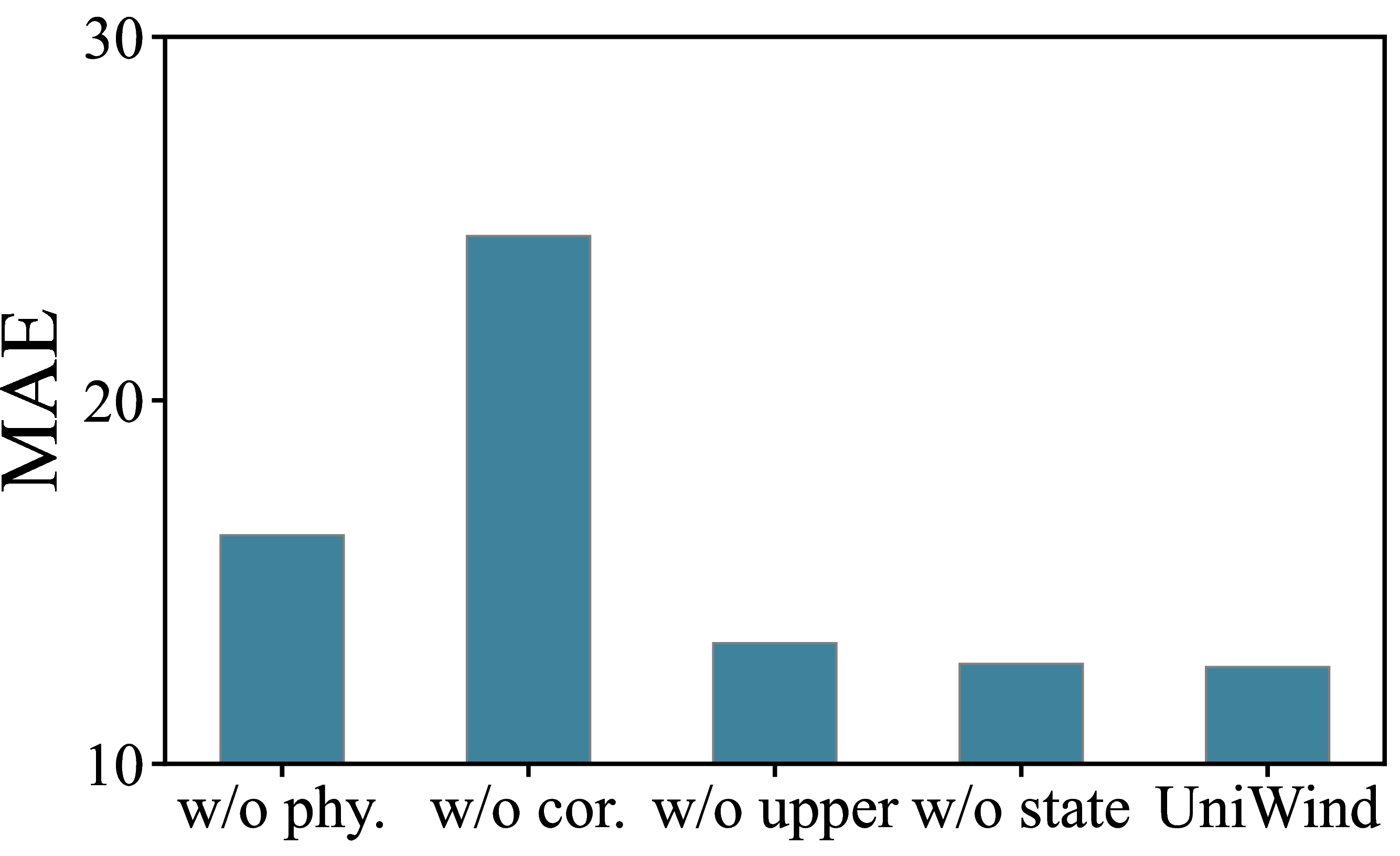
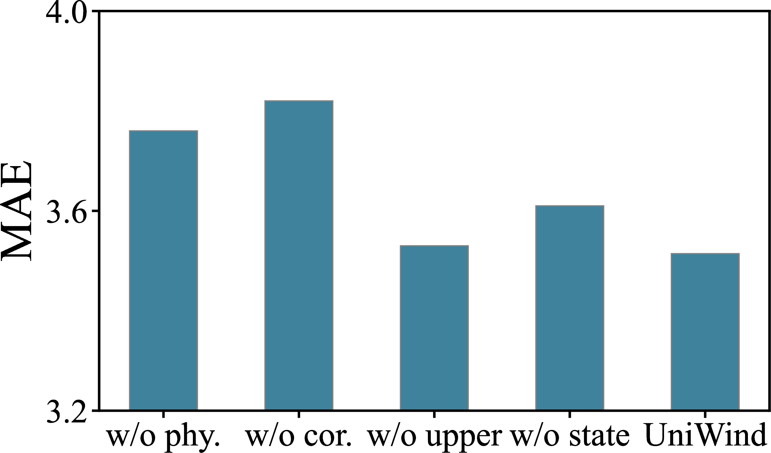
Figure 6: Ablation Studies..
9.3 State Statistics↩︎
Table 6 summarizes the average proportions of state-prior labels constructed by the procedure in Appendix 8.3. The regular state dominates all regions, but the proportion varies substantially, from 44.8% in the UK to 84.3% in AH. The abnormal states also show clear regional differences, indicating that wind farms in different regions exhibit distinct operating-state distributions.
| Region | Regular (%) | Shutdown (%) | Curtailment (%) |
|---|---|---|---|
| AH | 84.3 | 14.7 | 1.0 |
| SD | 61.0 | 34.0 | 5.0 |
| SX | 78.2 | 20.8 | 1.0 |
| UK | 44.8 | 18.0 | 37.2 |
9.4 Parameter Sensitivity Analyses↩︎
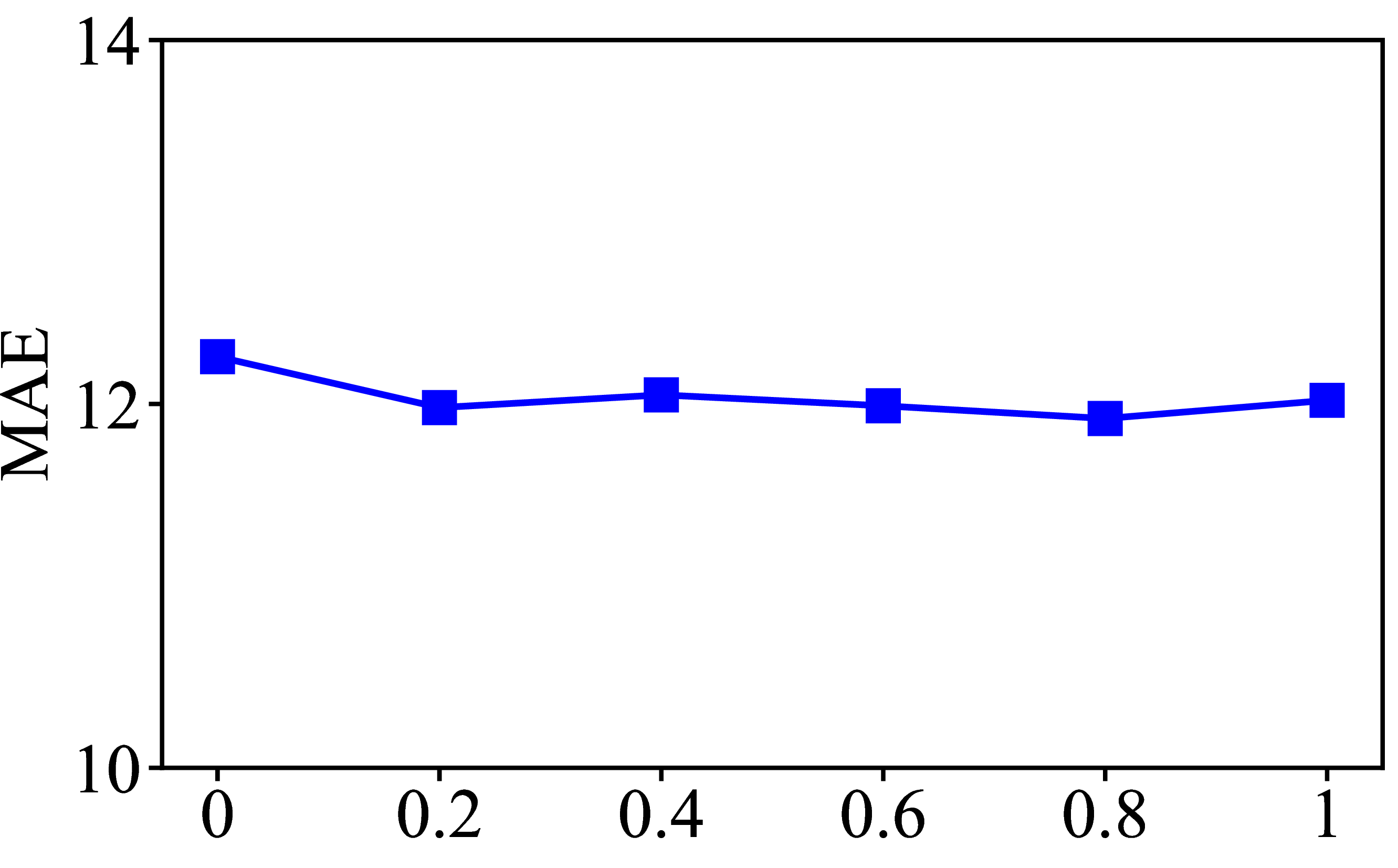
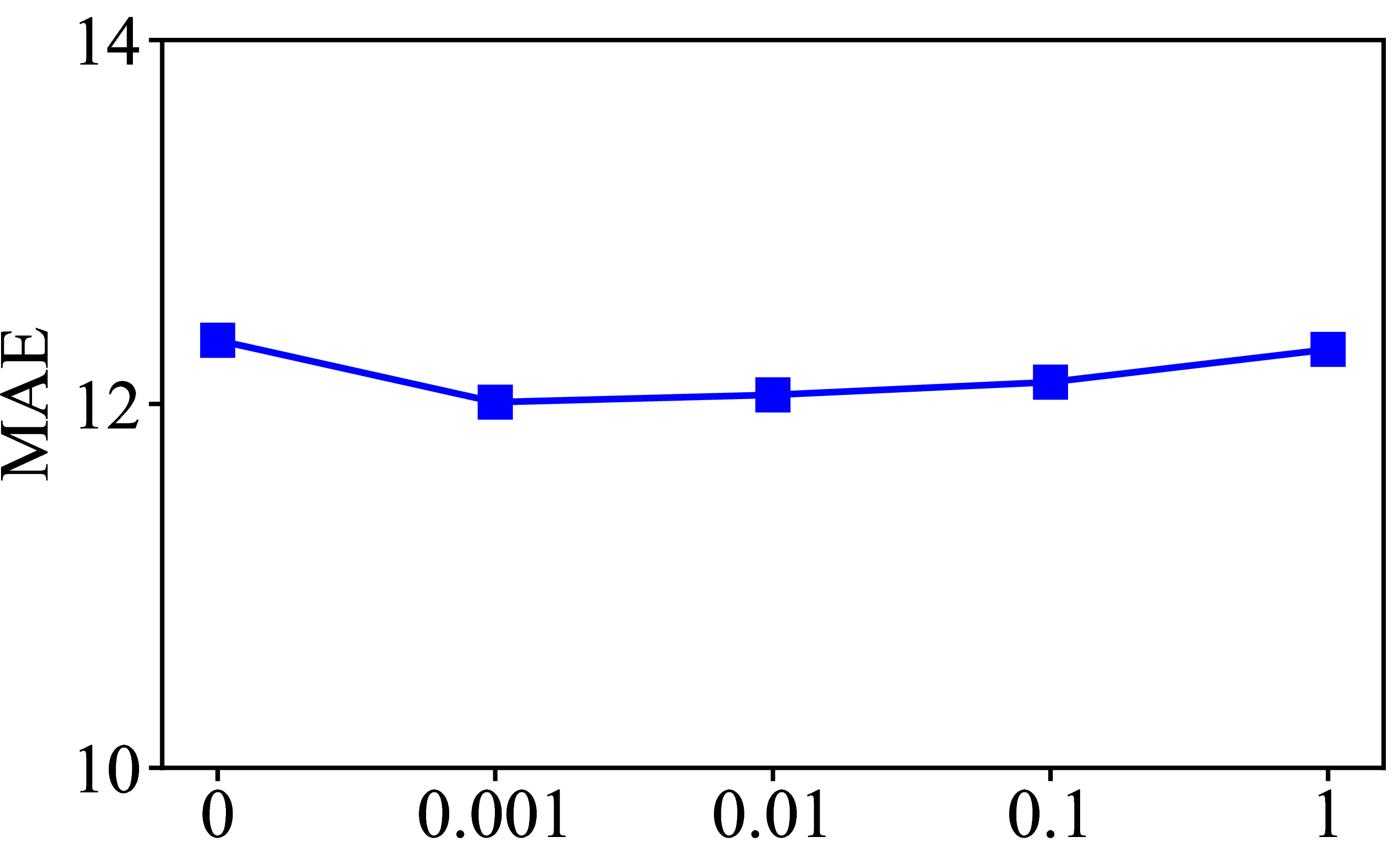
Figure 7: Sensitivity analysis on the SD_A dataset..
Figure 7 shows the sensitivity of UniWind to the router-supervision weight \(\lambda_{\mathrm{router}}\) and the physical upper-bound weight \(\lambda_{\mathrm{upper}}\) on the SD_A dataset. When either weight is set to 0, the MAE increases, indicating that both knowledge-guided state supervision and physical upper-bound regularization contribute to stable forecasting. For nonzero values, the performance remains relatively stable, suggesting that UniWind is not highly sensitive to the exact choice of these hyperparameters. Based on the validation performance, we set \(\lambda_{\mathrm{router}}=0.4\) and \(\lambda_{\mathrm{upper}}=0.01\) in the final model.
9.5 Case studies↩︎

Figure 8 provides a qualitative example on the SD_A dataset, illustrating how UniWind separates physically available power from realized generation. The physical prior generally follows the wind-speed profile: it increases rapidly when wind speed enters the productive range, decreases under low-wind conditions, and forms a plateau during high-wind periods. This plateau does not indicate a forecasting error, but reflects the saturation of the wind farm at its rated power after the wind speed reaches the rated region. However, the realized power can remain substantially below this available-power envelope because of latent operating conditions and site-specific effects. UniWind therefore does not directly use the physical prior as the final output. Instead, the State-aware Power Corrector adjusts the prior according to the inferred operating state, enabling the prediction to follow the ground-truth trajectory during both high-potential intervals and low-output periods. In particular, the prediction tracks the ground truth when the physical prior stays near the rated-power plateau, and also captures the sharp drops and recoveries when the available power changes rapidly. This case confirms that the proposed physical prior provides a meaningful upper-envelope reference, while state-aware correction is necessary to translate this reference into realistic day-ahead power forecasts.