pykci: A Compact Urban Knowledge Graph for Semantic and Spatial Queries using LLMs
July 02, 2026
Abstract
CityGML, the OGC standard for the modeling, storage, and exchange of semantic 3D city models, describes urban objects with detailed semantics, geometry, and topology. Yet this richness is difficult to query directly: CityGML’s XML encoding is designed for exchange rather than analysis, and relational mappings expose it through schemas that demand expert knowledge. We present pykci (Python Knowledge Graph for Cities), an open-source system that transforms CityGML 2.0 datasets into a compact urban knowledge graph in Neo4j and makes it queryable in plain natural language. The graph schema covers all thematic feature modules of CityGML 2.0 across all levels of detail and is spatially indexed with an R-tree for efficient geometric retrieval. A complete end-to-end Python pipeline ingests CityGML datasets into the knowledge graph, exports them to OGC 3D Tiles for interactive visualization, and supports lossless round-trip export of all modeled content back to CityGML. For querying, the graph is paired with a large language model through a model-agnostic text-to-Cypher mechanism: the graph schema is supplied as context, and the model translates natural-language questions into Cypher queries executed directly against the graph. We evaluate both a locally running open-weight model, which keeps sensitive city data on-premise, and a state-of-the-art commercial model for the most demanding spatial and semantic queries. Answers are thereby grounded in exact city data rather than the model’s parametric memory, reducing hallucination and providing auditable provenance for every response. We demonstrate the system on open-government CityGML LoD2 datasets from Hamburg, Germany, including complex semantic and spatial queries such as identifying roof surfaces suitable for greening. pykci enables urban planners, GIS practitioners, and citizens to interact with semantic 3D city models without expertise in query languages and database schemas.
<ccs2012> <concept> <concept_id>10002951.10002952.10002953.10010146</concept_id> <concept_desc>Information systems Graph-based database models</concept_desc> <concept_significance>500</concept_significance> </concept> <concept> <concept_id>10002951.10003227.10003236.10003237</concept_id> <concept_desc>Information systems Geographic information systems</concept_desc> <concept_significance>500</concept_significance> </concept> <concept> <concept_id>10010147.10010178.10010179.10010182</concept_id> <concept_desc>Computing methodologies Natural language generation</concept_desc> <concept_significance>300</concept_significance> </concept> </ccs2012>
1 Introduction↩︎
More than 4.2 billion people, over 55 % of the global population, live in cities today, and the United Nations projects this proportion will reach 68 % by 2050 [1]. Supporting this growth imposes increasing demands on infrastructure, urban planning, and data management. In Germany alone, the national 3D Building Model at Level of Detail 2 (LoD2-DE) already comprises 58 million buildings [2], each represented with detailed semantics, geometry, and topology: typed boundary surfaces, precise three-dimensional geometry, and thematic attributes such as function, roof form, and measured height. Such data increasingly forms the backbone of urban digital twins (UDTs), virtual replicas of the physical city used for planning, simulation, and decision-making [3], [4]. At the core of any UDT lies a queryable digital knowledge base, and how easily its encoded knowledge can be accessed by various stakeholders determines how useful the twin is in practice.
The City Geography Markup Language (CityGML) [5], an Open Geospatial Consortium (OGC) standard for modeling and exchanging urban objects and landscapes, is the de facto format for semantic 3D city models, but its XML encoding is designed for exchange rather than analysis. The most widely used backend, the 3D City Database (3DCityDB) [6], maps CityGML to a relational schema spanning many interrelated tables; retrieving semantically meaningful relationships, such as identifying buildings in a district suitable for roof greening given constraints on roof slope, type, and material, requires complex multi-join queries that scale poorly and obscure the data’s inherent structure. That structure is fundamentally graph-like: a building decomposes into boundary surfaces, then polygons, then points, and CityGML reuses shared geometry, such as a wall surface referenced by two adjacent rooms, through explicit references. Such deeply connected data is more naturally represented in a graph than in flat relations [7].
Graph databases store entities as nodes and relationships as first-class edges, enabling efficient traversal of connected data [8], and knowledge graphs (KGs) add a semantic layer of typed entities and relations [9], [10]. KGs are increasingly adopted as the integrating knowledge base inside UDTs [11]–[13]. We represent CityGML as a labeled property graph (LPG) in Neo4j rather than as Resource Description Framework (RDF) triples, a choice we motivate in 2; and while the closest prior system, 3DCityKG [7], also maps CityGML to a graph, it mirrors the verbose CityGML hierarchy, whereas we adopt a compact schema with shorter traversal paths.
A KG does not by itself lower the query barrier: users must still know the schema and a query language such as Cypher. Large language models (LLMs) promise a natural-language interface, but applying them directly to city models fails on two counts. A single city’s CityGML describes tens to hundreds of thousands of buildings, far exceeding practical context limits and prohibitive in token cost; and correct interpretation demands domain-specific knowledge, such as the distinction between a GroundSurface and a RoofSurface or the meaning of code-based function values, that general-purpose models lack. Embedding a city into the model itself, as in CityGPT [14], conflates the query interface with the data store and does not generalize across cities or updates. We instead keep the knowledge base external: the LLM receives the graph schema as context and generates Cypher that executes directly against the graph. This keeps context compact, lets the data be updated without retraining, and grounds every answer in exact, auditable graph data rather than the model’s parametric memory.
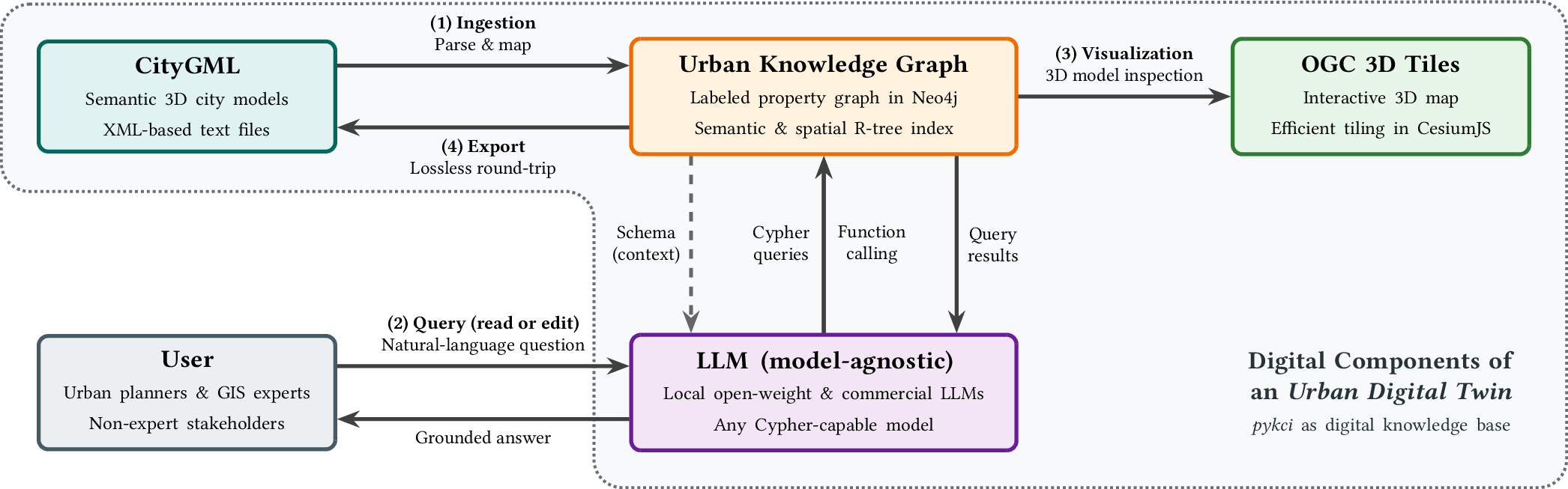
We present pykci (Python Knowledge Graph for Cities, pronounced pixie), a compact urban KG for CityGML 2.0, implemented as an LPG in Neo4j. The graph schema covers all thematic feature modules of CityGML 2.0, including buildings, bridges, tunnels, transportation, and vegetation, across all five levels of detail (LoD0–4), and incorporates an R-tree spatial index for efficient geometric querying. We provide a complete end-to-end pipeline in Python that ingests CityGML datasets into the KG, exports the result to OGC 3D Tiles for interactive 3D visualization, and supports round-trip export back to CityGML for editing workflows. For complex querying, the KG is paired with an LLM through a model-agnostic text-to-Cypher interface: a locally running open-weight model serves routine queries entirely on-premise, while a commercial model handles the most demanding reasoning when higher accuracy is required. The generated queries run directly against the graph, enabling urban planners and GIS practitioners to interact with 3D city data without query-language expertise. pykciis demonstrated on open-government CityGML LoD2 datasets from Hamburg, Germany, is released as open-source software, and, within the broader vision of UDTs, serves as the queryable digital knowledge base that makes a city’s semantic 3D model accessible to both software components and non-expert users. Our main contributions are: (1) a compact, semantically and spatially indexed urban KG schema for CityGML 2.0; (2) a fully open-source, end-to-end ingestion, visualization, and export pipeline in Python; and (3) a natural-language querying interface for complex semantic and spatial queries over large-scale 3D city models via LLM.
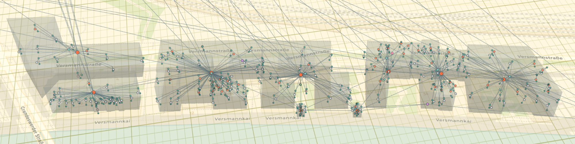
[fig:teaser] shows the resulting urban KG for the HafenCity district of Hamburg, spatially aligned with its CityGML LoD2 building models rendered as OGC 3D Tiles, while 1 gives an overview of the workflow, positioning pykcias the digital knowledge base of a UDT. 2 reviews related work; 3 presents the pykcischema and mapping rules; 4 evaluates the proposed mapping method based on well-known datasets; 5 assesses the performance and efficiency of pykciagainst related tools; 6 demonstrates real-world LLM-based querying use cases; and 7 concludes.
2 Related Work↩︎
This section briefly reviews prior work related to pykci: semantic 3D city models, CityGML data model, relational and graph representations of CityGML, urban KGs and UDTs, and LLMs in combination with spatially-enhanced KGs.
2.1 Semantic 3D City Models and CityGML↩︎
CityGML [5] is the OGC standard for representing, storing, and exchanging semantic 3D city models, and one of the key data models for urban digital twins. Unlike conventional 3D city models, which capture only graphical or geometrical representation, CityGML jointly encodes the semantic, topological, geometrical, and appearance properties of city objects in a single model. It is an application schema of GML 3.1.1 [15], the OGC’s XML grammar for geographic features defined in line with ISO/TC 211. Released in successive versions (1.0 in 2008, 2.0 in 2012, and 3.0 in 2021 [16]), CityGML has become the most widely used exchange format for semantic 3D city models. It has been adopted in more than 20 countries [17], including Japan, Australia, Germany, the United Kingdom, and the United States. This paper focuses on CityGML 2.0, which remains the most widely adopted version and accounts for the majority of open-government datasets, including the dataset used in this study. Unless stated otherwise, the term “CityGML” hereafter refers to version 2.0. Alternative encodings exist: CityJSON [18] provides a compact JSON serialization of a subset of CityGML’s data model, while OpenStreetMap (OSM) offers crowd-sourced but largely LoD1 building data and street networks.
CityGML [5] represents a city as a collection of city objects organized into thematic modules (Appearance, Bridge, Building, CityFurniture, CityObjectGroup, Generics, LandUse, Relief, Transportation, Tunnel, Vegetation, WaterBody, and now-deprecated TexturedSurface) and across five levels of detail (LoD0–4). A building is bounded by typed boundary surfaces, namely GroundSurface, WallSurface, and RoofSurface, each described by one or more polygons. A polygon is defined by an exterior ring and optional interior rings, and rings are ordered lists of points. This yields a strict containment hierarchy that at first appears tree-like. In practice, however, geometry can be shared between features through references (XLinks), so that a single surface instance is defined once and reused by multiple objects. The data model is therefore a graph rather than a tree [19].
To enable this semantic and structural richness, CityGML employs a complex, multi-level class hierarchy in which elements are defined at different levels of abstraction [5]. It makes extensive use of object-oriented principles such as inheritance, encapsulation, and polymorphism. In contrast, graph databases such as Neo4j, like many other database systems, are instance-based [8], meaning they primarily store instances of classes rather than explicit class definitions. Another challenge arises from the permissive nature of the GML and CityGML encoding standard, which allows multiple syntactic representations for the same object [7]. For example, a surface can be represented either as a single polygon or as a collection of smaller adjacent polygons that together form the same geometry. This syntactic ambiguity complicates the conversion between CityGML and graph-based data models, particularly when aiming to produce a compact graph representation, such as pykci.
2.2 Database Representations of CityGML↩︎
Representing CityGML in a database poses several challenges. Production datasets are large, reaching tens of millions of buildings [2]; the model has a deep class hierarchy; geometry is frequently shared between features through references (XLinks); and the underlying encoding schemas allow several syntactic ways to define the same object. Together, these properties render traditional relational or document storage either lossy or inefficient for complex analytical querying.
Relational databases remain the most widely used backend for semantic 3D city models. 3DCityDB [6] maps CityGML to many interrelated tables and is well suited to storage and exchange, but recovering semantic relationships requires multi-join queries that obscure the data’s connected structure. To better preserve this structure, object-oriented and graph-based mappings have been proposed.
Two graph paradigms dominate. In the semantic-web tradition, CityGML is mapped to RDF triples with ontologies in the Web Ontology Language (OWL) and GeoSPARQL as the spatial query interface [20], [21], enabling linked-data integration and ontology reasoning. However, standard RDF cannot attach properties to edges [22]. Encoding the attributes of a relationship instead requires reification, which inflates triple counts and complicates querying. Such relationship attributes are common in 3D city models, for example, the ordering of boundary surfaces within a building and the XLinks present in the original CityGML dataset. pykcipreserves these natively as edge properties for reconstruction of CityGML on export. The RDF-star extension [23] allows triple annotation by allowing statements about statements, but its support across triplestores and GeoSPARQL implementations remains uneven. It also does not alter RDF’s separation of spatial evaluation from graph traversal: GeoSPARQL evaluates spatial predicates over geometry literals such as Well-known Text (WKT) via filter functions [24] rather than as native graph traversal primitives.
In the LPG tradition, 3DCityKG [7] maps CityGML to a Neo4j graph with high-performance, multi-threaded ingestion. Its graph mirrors the CityGML class hierarchy, which enables lossless round-trip export and intuitive navigation for domain experts, but places content nodes many hops below their top-level features, increasing traversal depth and the context cost of querying. Originally designed for automatic change detection and interpretation of large semantic 3D city models within the tool citymodel-compare [7], [25], 3DCityKG features an in-memory spatial index for efficient online graph matching, but the persistent graph cannot leverage it in its current version [26]. The appropriate representation thus depends on the use case: exchange and archival favor 3DCityDB, ontology integration favors RDF, and analytical traversal, spatial querying, and compact LLM context favor a purpose-built LPG. pykcifollows the last direction with a deliberately compact schema.
2.3 Neo4j, Cypher, and Spatial Indexing↩︎
Neo4j is a graph database that implements the LPG model [8]. It stores nodes and relationships with native pointers (index-free adjacency), allowing constant-time traversal of relationships independent of dataset size. Graphs are queried in Cypher, a declarative, pattern-based query language in which queries specify subgraph patterns to match. For example, the following query retrieves all buildings together with their roof surfaces:
MATCH (b:Building)-[:HAS_BOUNDARY]->(s:RoofSurface)
RETURN b, s
In addition to the built-in labeled-base semantic and point indexes, pykciuses the Neo4j Spatial extension [27], which maintains an R-tree index over feature 2D bounding boxes and exposes spatial predicates such as bounding-box, intersection, and within-distance search. The combination of pattern-based traversal and spatial indexing allows a single query to express both semantic conditions (for example, roof type) and spatial conditions (for example, proximity to a location) over the same graph.
2.4 Urban Knowledge Graphs and Digital Twins↩︎
The term “knowledge graph” has no single agreed definition [9], [28]–[30]. We adopt the definition of Hogan et al. [9]: a knowledge graph (KG) is “a graph of data intended to accumulate and convey knowledge of the real world, whose nodes represent entities of interest and whose edges represent relations between these entities.” A KG thus adds a semantic layer to a graph by fixing the meaning of node and edge types through a schema or ontology [10]. Surveys of the field [10], [31] distinguish general or world KGs, such as DBpedia [32], Wikidata [33], and YAGO [34], from domain-specific KGs. Urban KGs apply the concept at city scale: UrbanKG [35] fuses regions, points of interest, and mobility data to support traffic prediction and site selection, while UrbanKGent [36] uses LLMs to assist urban KG construction. Reviews note that smart-city domain KGs remain at an early stage of development [31]. KGs are increasingly used as the integrating knowledge base of UDTs [4], [11]–[13], linking heterogeneous data into a queryable structure. Most existing urban KGs, however, emphasize point-of-interest and mobility data rather than the detailed geometric and semantic content of CityGML LoD2 models, which is the focus of our work.
2.5 LLMs and Spatial Knowledge Graphs↩︎
LLMs and KGs are increasingly combined. [10] survey this synergy, observing that KGs supply external, updatable, and interpretable knowledge while LLMs contribute language understanding, and that KGs are by nature difficult to construct and evolve. Retrieval-augmented generation (RAG) [37] grounds LLM outputs in retrieved external data, and GraphRAG [38] extends this to graphs built from unstructured text. Our setting differs fundamentally: the graph is an authoritative, schema-defined city model queried through a text-to-Cypher mechanism, not a corpus of retrieved text fragments. Recent work questions the need for pre-built graphs in RAG altogether [39], while others target the spatial-reasoning limitations of LLMs [40]. For city models specifically, CityGPT [14] fine-tunes a city-scale world model into the LLM.
Some recent related systems, like pykci, expose CityGML to natural-language querying. KCitychatBot [26] couples a multi-agent LLM pipeline with a CityGML KG in Neo4j, constructed with a hierarchical mapping in the 3DCityKG tradition [7], on large-scale CityGML data. The chatbot generates Cypher but does not support spatial analysis, which its authors defer to future work using external tools such as PostGIS, and it relies on an embedding model for intent extraction. [41], [42], by contrast, support spatial and temporal querying and 3D Tiles visualization, but store the city model in the relational 3DCityDB and translate user questions into SQL, supplying the LLM with a multi-table relational schema serialized as several hundred lines of context. pykcioccupies the gap between these: it queries a compact, spatially indexed CityGML property graph through text-to-Cypher, enabling spatial predicates such as proximity, intersection, and containment to be combined with semantic traversal in a single query. The schema is sufficiently compact to fit within the model’s context and does not require embeddings on the query path.
3 Graph Schema and CityGML Mapping↩︎
We present the graph schema employed by pykci and formalize the transformation rules used to map a CityGML dataset into an LPG.
3.1 Design Principles↩︎
The schema is guided by five principles.
3.1.1 Directed acyclic structure.↩︎
pykcirepresents the city as a directed acyclic graph (DAG), with edge directions aligned to CityGML semantics. Aggregation and composition (“part-of”) relations consistently point from higher-level entities to their constituents (such as from building down to surface, polygon, and ring). This orientation allows queries, including those generated by LLMs, to infer traversal direction quickly based on local node and edge labels, independently from global schema. Although CityGML may permit directed cycles (e.g., upward XLinks), such cases are rare and absent in our datasets. Enforcing acyclicity thus preserves observed information while guaranteeing termination of recursive traversals.
3.1.2 Compactness.↩︎
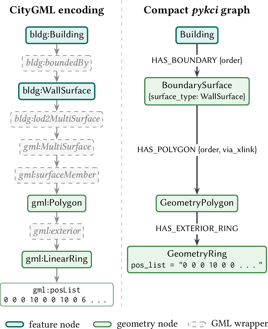
Traversal paths are shortened by mapping only semantically meaningful CityGML elements to nodes, centralizing them around top-level feature nodes (like buildings), and collapsing wrappers in the CityGML serialization. This contrasts with
hierarchy-faithful mappings such as 3DCityKG [7] and significantly reduces both query hops and the amount of context an LLM must
process, as illustrated in 2. By a wrapper, we refer to an intermediate GML element (e.g., gml:surfaceMember, gml:exterior) that only groups or nests geometry and carries neither content nor an
identifier of its own.
3.1.3 Losslessness.↩︎
Every identifier, thematic attribute, ordering, XLink indicator, and coordinate string is preserved, enabling exact reconstruction of the original CityGML (3.3). While compactness and losslessness appear conflicting, since faithful reconstruction tends to require materializing every wrapper, we resolve this with a single rule: information needed only for serialization is stored as node or edge properties, not as additional nodes.
This yields three consequences. (1) Semantic content (e.g., city objects, rooms, openings, boundary surfaces, and geometry hierarchies) is represented as nodes and edges, with their order among sibling elements stored as the edge property
order. (2) XLink references are modeled as explicit edges, annotated with a property via_xlink set to true, to support CityGML reconstruction. Thus, wrappers are reduced to edge properties, preserving one-hop
references. (3) Irregular or open-ended leaf data, such as pos_list, xAL addresses, metadata, and Application Domain Extension (ADE) content, is stored verbatim as string properties and reattached during export rather than modeled
structurally.
3.1.4 Dataset idempotency.↩︎
Ingestion uses Cypher’s MERGE clause, which combines MATCH and CREATE: it first searches for a node pattern and creates it only if absent. As a result, re-ingesting a dataset does not produce duplicates, and shared
geometries are merged into single nodes. This is particularly beneficial for XLink resolution. During mapping, an XLink may refer to an element that has not yet been encountered, which would require collecting all references first before matching. With
MERGE, referenced nodes are created on first mention and enriched later, eliminating the need for deferred-reference lists and post-processing.
3.1.5 Spatial indexing.↩︎
Location queries, such as retrieving features within a bounding box or near a point, would otherwise require a full label scan with a per-node coordinate comparison. To avoid this, in addition to Neo4j’s built-in point index on feature centroids, an
R-tree spatial index is employed. It registers every top-level feature that has a gml:boundedBy envelope (Building and all CityObject subtypes) by its 2D bounding box. The box is stored in WKT format as a node
property, which can be parsed by the R-tree layer.
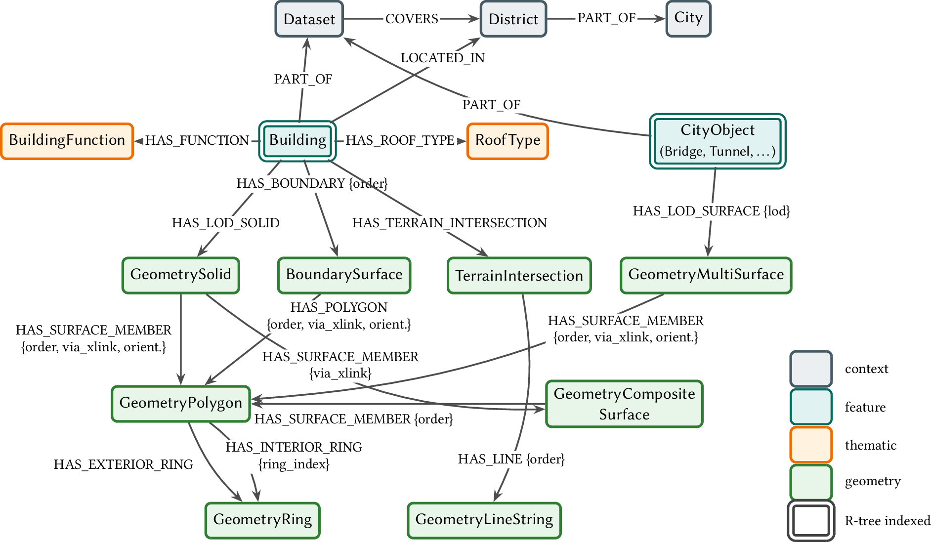
The core graph schema is summarized in 3. 4 illustrates how Building elements are mapped to graph entities using the schema and mapping rules defined in this work.
![Figure 4: Content composition of a CityGML Building object. Properties are grouped by their defining class, with the class hierarchy shown at the bottom. Property types follow the Java bindings of the citygml4j parser. All substantial content can be mapped to graph using pykci’s own graph schema: mapped to a dedicated node or subgraph, stored as a node property, stored verbatim as an XML subtree (opaque to queries), and represented as an edge to a shared node. denotes elements outside the scope of this work (e.g., parser artifacts or the excluded Appearance module). Adapted from [7].](/article/2607.01605/_pdflatex/icftazbk.png "fig:")
3.2 Mapping CityGML to Graph↩︎
The schema defines five node groups. (1) Feature nodes represent CityGML city objects, including top-level features like Building, Bridge, and Tunnel. Notably, the model supports recursive structures
through the BuildingPart node, which is connected to a Building via a HAS_BUILDING_PART edge and reuses the full Building geometry modeling schema. (2) Interior feature nodes extend the schema to
support LoD3–4 representations, including Room, BuildingInstallation, BuildingFurniture, and Opening (covering doors and windows). (3) Geometry nodes represent the hierarchical spatial
decomposition of objects. These include GeometrySolid, GeometryMultiSurface, GeometryCompositeSurface, BoundarySurface, GeometryPolygon, GeometryRing,
GeometryLineString, and TerrainIntersection. (4) Thematic nodes capture semantically significant attributes, particularly code-list values such as BuildingFunction and RoofType. Due to their
potentially high query frequency, these values are modeled as standalone nodes rather than node properties. Identical values are stored once and shared across all referencing features (via MERGE), allowing for explicit, queryable
relationships. For instance, selecting a BuildingFunction node indicating residential use enables efficient retrieval of all associated buildings via their connecting edges. (5) Context nodes (e.g., Dataset,
District, City) represent information within administrative and provenance contexts. The City node is derived from the CityModel element in the CityGML document, while Dataset and
District nodes are introduced based on available metadata of the dataset.
Relationships are divided into three categories. (1) Decomposition edges encode geometric and part–whole containment, including HAS_LOD_SOLID, HAS_BOUNDARY, HAS_POLYGON, HAS_SURFACE_MEMBER,
HAS_EXTERIOR_RING, HAS_INTERIOR_RING, HAS_LOD_SURFACE, and HAS_LINE. Interior nodes have their own edges, including HAS_INTERIOR_ROOM, HAS_OPENING, and
HAS_BUILDING_PART. Edges may contain properties reserved for CityGML reconstruction: order (position among siblings), via_xlink (XLink indicator), orientation (for gml:OrientableSurface), and
ring_index (for position of interior rings in a polygon). (2) Classification edges like HAS_FUNCTION and HAS_ROOF_TYPE link a feature to its shared thematic nodes. (3) Context edges (e.g.,
PART_OF, LOCATED_IN, and COVERS) attach features to their dataset, district, and city.
3.3 Export from Graph↩︎
pykciserves as an operational data store and supports export to two formats. For interactive visualization, geometry is exported as an OGC 3D Tiles 1.1 [43] dataset (tileset.json with binary glTF tiles) and rendered in CesiumJS. The coordinate reference system (CRS) and geoid undulation are derived from the node properties srsName in the graph,
surfaces are triangulated, and per-feature identifiers are embedded in the GLB visualization files. This tileset provides the spatial context in [fig:teaser].
For data exchange, the export reconstructs a schema-valid CityGML 2.0 document covering all ingested modules and levels of detail. Since identifiers, ordering, typed attributes, code spaces, coordinate strings, and XLink relationships are preserved
during ingestion, the output restores geometry, semantics, and metadata, including LoD geometries, boundary surfaces, openings, building parts, installations, and interiors. The result is semantically complete with respect to the source (it contains every
element, attribute, text value, and coordinate of the input), enabling round-trip workflows. The appearance module (app:Appearance) is excluded.
4 Evaluation Results↩︎
We define a round trip as lossless in terms of semantic completeness: every element, attribute, leaf text value, and coordinate in the source must appear in a valid CityGML export, although encoding (e.g., gml:pos
vs.posList), element order, and whitespace may differ. To measure this property, an automated census parses the source and the export and reduces each document to four multisets: element local-names, (attribute, value) pairs,
(element, text) pairs, and coordinate tokens. A coordinate token is an individual scalar value parsed from gml:pos or gml:posList. The export covers the source if and only if every source multiset is contained in the
corresponding export multiset. We apply the census on two axes: all LoDs (4.1) and the thematic feature modules (4.2).
4.1 Mapping All Levels of Detail (LoD0–4)↩︎
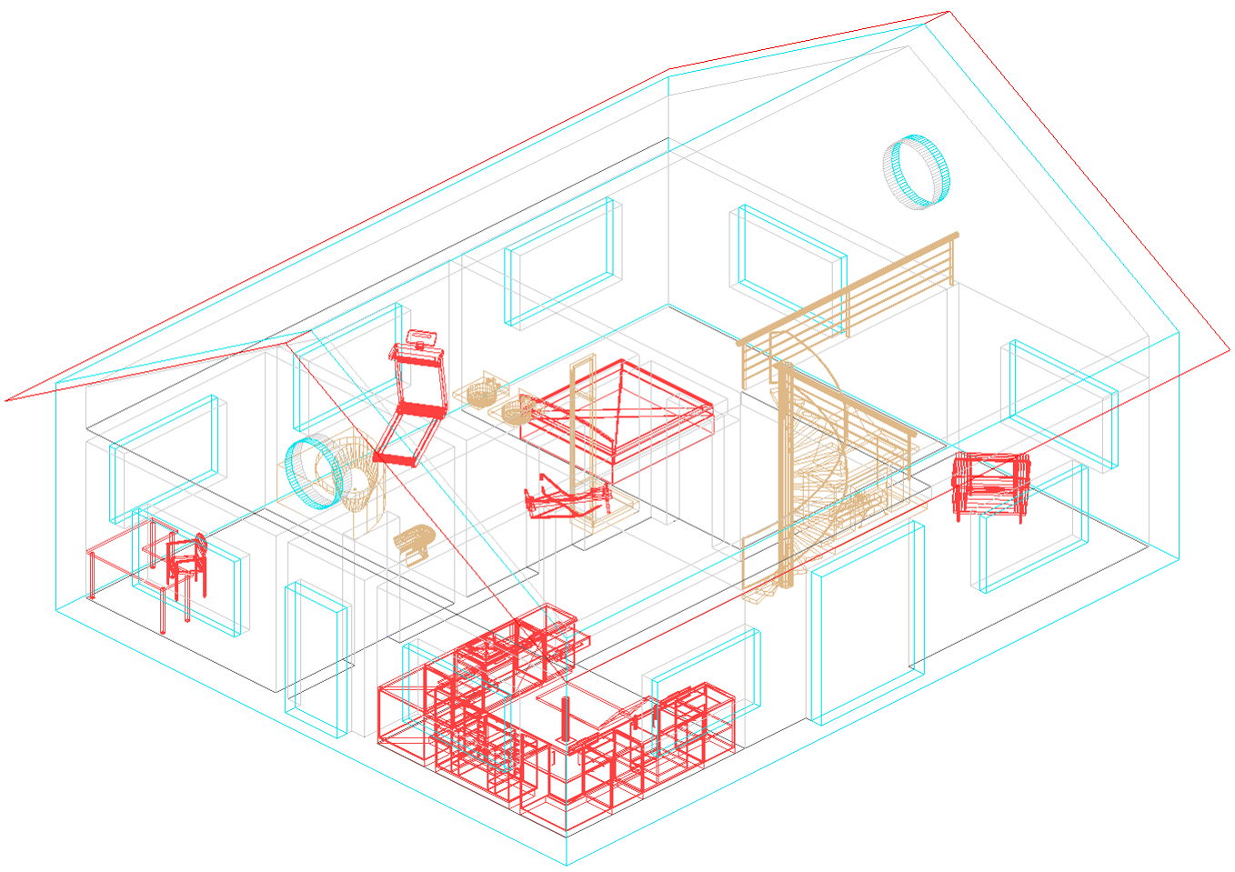
We use the FZK-Haus reference building published by KIT [44] in all five LoD0–4. These datasets contain per-vertex coordinates, identifiers, composite and orientable surfaces, and, at LoD4, a complete interior of rooms, furniture, and installations (see 5). For each LoD, we execute the pipeline end to end, ingesting the source into Neo4j and exporting it back to CityGML, and then census the source against the export. 1 counts every source instance by category and reports the fraction that the export covers. The source grows by more than three orders of magnitude across the LoDs, from 117 instances at LoD0 to 275366 at LoD4, where the interior elements dominate. The mapping covers 100 % of the instances at every LoD.
| LoD | Elem. | Attr. | Text | Coord. | Source total | Coverage |
|---|---|---|---|---|---|---|
| 0 | 49 | 16 | 22 | 30 | 117 | 100 % |
| 1 | 65 | 16 | 22 | 90 | 193 | 100 % |
| 2 | 112 | 23 | 30 | 111 | 276 | 100 % |
| 3 | 1036 | 36 | 43 | 4191 | 5306 | 100 % |
| 4 | 59699 | 208 | 194 | 215265 | 275366 | 100 % |
4.2 Mapping the Thematic Feature Modules↩︎
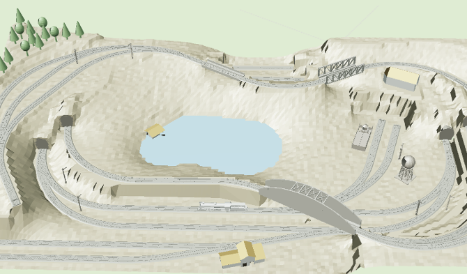
To evaluate mapping of thematic modules beyond buildings, we employ the Railway Scene dataset in LoD3 [45], which packs 52 top-level features from ten CityGML modules into a single scene (see 6). These include the modules Bridge and Tunnel with nested construction elements and installations, a native Triangulated Irregular Network (TIN) relief, XLink-based group membership, and generic city objects. We ingest the whole scene, export it, and census the source against the export over the entire document. ¿tbl:tab:census95railway? lists the modules and the distinctive elements that each contributes. A check mark indicates that the module’s content has been mapped within the fully covered scene. In total, the census counts 1182102 source instances (243254 elements, 487 attributes, 1194 text values, and 937167 coordinate tokens), and the export covers all of them (100 %). Ten CityGML 2.0 thematic feature modules appear in this scene. The eleventh module, LandUse, is supported by the same surface-only geometry mapping as Transportation but is not available in any of the evaluation datasets. The only non-feature module Appearance is out of scope by design.
@lrXc@ Module & Feat. & Distinctive elements & Cov.
Building & 3 & openings, installations & ✔
Bridge & 4 & nested con. ele., installations & ✔
Tunnel & 4 & nested installations, closure & ✔
Transportation & 10 & surface-only LoD railway & ✔
Vegetation & 15 & solitary obj., lodN geometry & ✔
CityFurniture & 11 & lodN geometry & ✔
WaterBody & 1 & water boundary surfaces & ✔
Relief & 1 & native triangulated surfaces & ✔
CityObjectGroup & 1 & XLink group membership & ✔
GenericCityObject & 2 & typed generic attributes & ✔
Elements & & 100 %
Attributes & & 100 %
Text & & 100 %
Coords & & 100 %
Total & & 100 %
5 Benchmarking Results↩︎
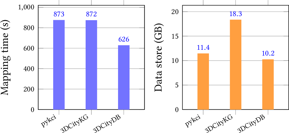
We evaluate the performance of pykciagainst two open-source CityGML database mappers: 3DCityKG 1.0 [7] (graph-based, Neo4j) and 3DCityDB 5.0 [46] (relational, PostgreSQL/PostGIS). All three systems ingest the same \(6.93\,\mathrm{GB}\) CityGML 2.0 LoD2 dataset of Hamburg [47], comprising \(388{,}267\) buildings recorded in 2025. To ensure a fair comparison, each system is executed in Docker under identical hardware conditions (8 logical CPU cores at 4.7–5.2 GHz and \(20\,\mathrm{GB}\) RAM), reads the dataset via the same bind mount, and is benchmarked over three runs (run-to-run variance under \(3\%\)). We report mean mapping wall-clock time as well as the resulting database size and graph entity counts.
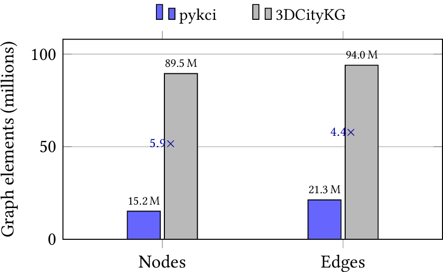
As shown in 7, pykcimaps the dataset in \(873\,\mathrm{s}\) (\(15\,\mathrm{min}\)), statistically indistinguishable from 3DCityKG (\(872\,\mathrm{s}\)). The relational 3DCityDB is the fastest at \(626\,\mathrm{s}\). pykciis written in Python, while 3DCityKG and 3DCityDB are Java-based. In terms of storage, the pykci data store occupies \(11.4\,\mathrm{GB}\), approximately 40 % smaller than 3DCityKG at \(18.3\,\mathrm{GB}\), while the relational 3DCityDB is slightly smaller at \(10.2\,\mathrm{GB}\). Both pykci and 3DCityDB include spatial indexing (R-tree and Generalized Search Tree (GiST), respectively), whereas 3DCityKG does not store a persistent spatial index. As shown in 8, pykci employs a condensed semantic schema, yielding nearly 6 times fewer nodes and more than 4 times fewer edges compared to 3DCityKG. For the same dataset, the relational 3DCityDB requires 27 million rows across 4 populated tables.
We evaluate the performance of pykci, 3DCityKG, and 3DCityDB using 20 predefined natural-language questions, comprising 10 citizen-oriented queries (e.g., roof materials, tallest buildings) and 10 expert-oriented queries (e.g., spatial aggregates, solar scoring). The evaluation is conducted on the same Hamburg CityGML LoD2 model enriched with building roof materials (see 6). We employ LLMs as text-to-query interfaces, including both local open-weight and commercial models. We evaluate three local models: Gemma 4, Mistral Medium 3.5, and Qwen3.5 (4). Results obtained with Claude (Opus 4.8) are summarized in 2. The results show that pykci produces the shortest queries on average (approximately 290 characters) and achieves the fastest net database query time at 0.37 s (wall-clock time excluding client startup overhead). Both the full list of natural-language questions and a detailed per-query performance evaluation across all databases can be found in ¿tbl:tab:query-list? and ¿tbl:tab:query-detail? in the Appendix, respectively.
| pykci | 3DCityKG | 3DCityDB | |
| (Neo4j) | (Neo4j) | (PostGIS) | |
| Query language | Cypher | Cypher | SQL |
| Questions solved correctly\(^{a}\) | 20/20 | 20/20 | 20/20 |
| Schema-discovery queries\(^{b}\) | 2 | 7 | 3 |
| Authoring difficulty (1–5)\(^{c}\) | 2.1 | 3.9 | 2.0 |
| Mean query length (chars) | \(\sim\)290 | \(\sim\)460 | \(\sim\)970 \(^{d}\) |
| Net DB query time (mean)\(^{e}\) | 0.37 s | 2.10 s | 2.62 s |
| Spatial index at query time | R-tree | none | GiST |
6 Use Cases: Graph-based Enrichment↩︎
This section demonstrates how pykcican be used as a knowledge base to support real-world workflows, specifically for enriching city models with additional data. This includes roof material classification and the extraction of facade openings from imagery. To illustrate this, we use the same Hamburg KG introduced in 5.
6.1 Roof Material Enrichment↩︎
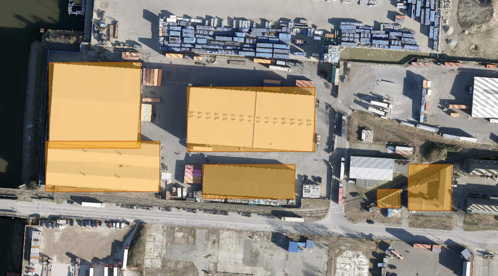
We attach deep learning based roof material predictions from a companion GeoJSON dataset, following the methodology of [48], to
almost half of the 388,267 Building nodes. The pykciKG remains compact, with only five additional nodes representing the roof material classes. Buildings with assigned roof material are linked to these nodes via
HAS_ROOF_MATERIAL relationships. Based on the enriched roof materials, further analysis and visualization can be performed. For example, these properties can be mapped alongside orthophotos to visually verify the prediction of such attributed
materials, as illustrated in Figure 9.
6.2 Facade Opening Enrichment (LoD3)↩︎
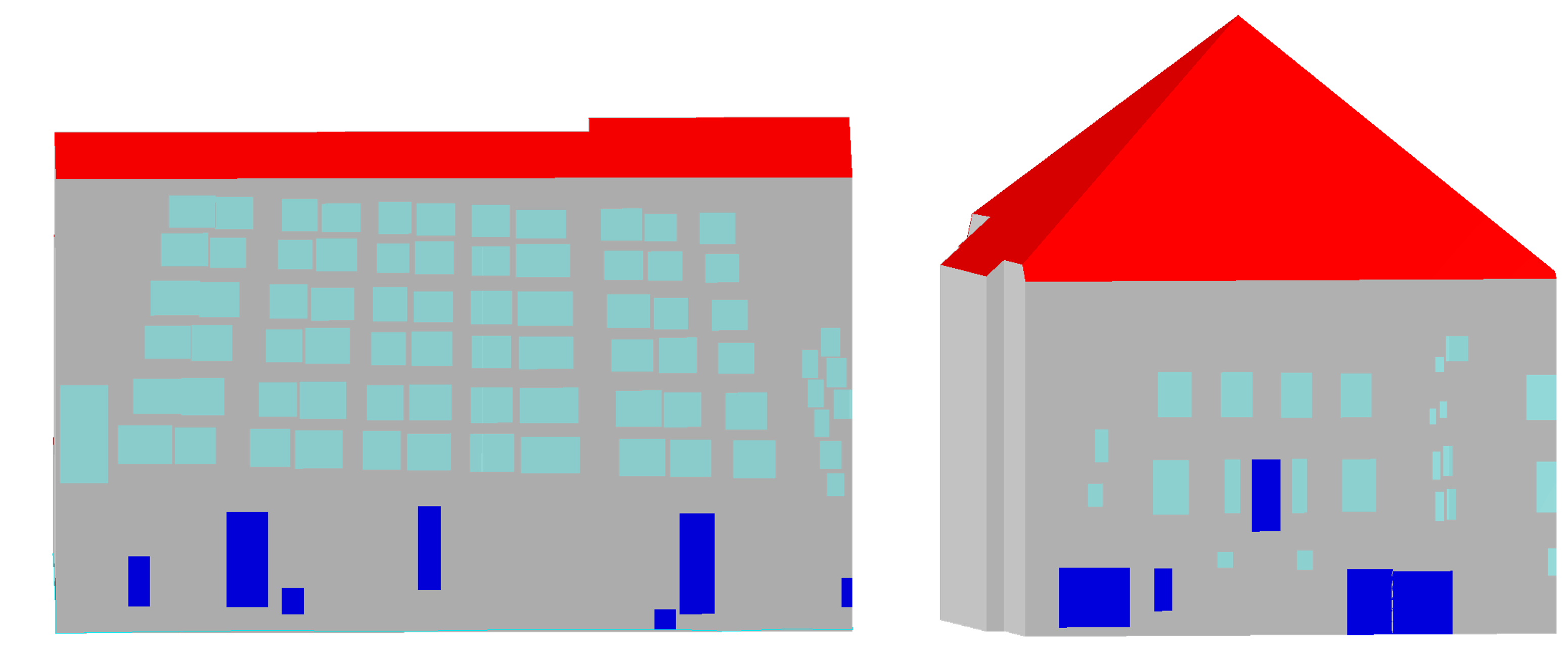
For 17 buildings in Hamburg, we derive their facade openings (i.e., window and doors), including position and shape, from RGB segmentation masks. 10 visualizes such detected windows in cyan
and doors in blue. Our approach maps bounding boxes to normalized UV coordinates in \([0,1]^2\), following the CityGML convention, where \(v = 0\) corresponds to ground level. Facade
openings are represented as nodes, each defined by normalized \(u\) and \(v\) coordinates and a semantic type. Similar to roof materials, these opening nodes are connected to buildings via
HAS_FACADE_OPENING edges. We intentionally adopt HAS_FACADE_OPENING instead of the canonical (BoundarySurface)-[:HAS_OPENING]->(Opening) pattern, as assigning openings to individual surfaces requires camera
calibration data that is not available in this dataset.
6.3 Downstream Applications in Urban Context↩︎
Greening planning and heat island mitigation.We aggregate dark roofing materials, primarily tar paper and metal, over a 2 km grid to derive a dark-roof fraction per grid cell. The maximum value, 49 %, occurs in the HafenCity port area and is consistent with the high density of industrial buildings. This screening approach provides a lightweight, spatially explicit indicator that integrates seamlessly with urban climate modeling. Building on the study of [48], [49] enrich CityGML datasets with footprint-guided roof-material labels and use these annotations to derive scene-specific land surface temperature (LST) estimates. Their framework enables the evaluation of cool-roof and green-roof retrofit scenarios and reports simulated citywide cooling effects of approximately 0.75 K in Hamburg, 0.62 K in Madrid, and 0.22 K in Paris. Since all enriched roof materials and facade openings are directly linked to buildings, as with other elements according to the pykcigraph schema, retrieving and processing climate-relevant data can therefore be performed in a single graph traversal with one hop.
Solar scoring. Another application of the enriched semantic property graph is photovoltaic (PV) suitability assessment. We compute a composite score that combines roof type, material, slope, and building height to rank buildings for solar
installations. Flat roofs made of glass or concrete and located at heights of at least 5 m receive the highest scores. Because buildings sharing the same roof material are connected, queries over material classes can be performed efficiently. This enables
direct use of material properties within graph-based ranking queries, for example through a single lookup within a reduce() expression.
Facade typology. Texture coordinates UV support facade-level analysis even in the absence of complete 3D geometry. The ratio of windows to doors can serve as an indicator of building function, with higher values typically associated with residential buildings. In addition, discretizing the vertical coordinate \(v\) into height intervals provides an approximation of opening density across different building levels. These derived metrics can be used as inputs to daylight availability assessments, occupancy estimation, and building energy-demand models. In addition, the resulting daylight and environmental noise simulations can serve as prior information for identifying suitable locations and strategies for urban densification, helping to balance development potential with environmental quality. 3 summarizes the information introduced in this section that can be added to pykcito support further analyses.
| Roof material | Facade openings | |
|---|---|---|
| Source | predicted GeoJSON | reconstructed CityGML |
| Pattern | HAS_ROOF_MATERIAL | HAS_FACADE_OPENING |
| Nodes/edges | 5 / 195,395 | 499 / 499 |
| Runtime | 15 s | 7.8 s |
| Applications | UHI, solar, V2X | typology, daylight |
7 Conclusion↩︎
We presented pykci, an open-source, end-to-end Python system that maps CityGML 2.0 datasets into a compact Neo4j-based urban KG, supports export to OGC 3D Tiles and lossless reconstruction to CityGML, and enables natural-language querying via a model-agnostic text-to-Cypher interface. The graph schema covers all thematic feature modules and LoDs. It integrates both semantic, as well as spatial point and R-tree indexing, allowing for efficient semantic and spatial querying. We evaluated and demonstrated the system on Hamburg CityGML LoD2 data, including complex tasks such as identifying roof surfaces suitable for greening, with results grounded in exact graph data.
pykcioffers several advantages. Its compact schema reduces LLM context size and enables exact query answering via Cypher rather than approximate similarity search, allowing small open-weight models to handle routine queries. The backend is interchangeable, enabling deployment across cities without retraining. Furthermore, the knowledge base remains local and private, requiring no tokenization or embedding of city data during query processing. However, the approach relies on an online database as external memory and abstracts away CityGML’s data model structure. While this improves semantic query efficiency, it reduces suitability for fine-grained structural comparison of city objects, such as sub-graph matching, which remains better supported by hierarchy-preserving mappings such as 3DCityKG.
Within UDTs, pykciserves as a knowledge base that is accessible to both software components and stakeholders. It provides a centralized platform for storing and integrating heterogeneous urban data. In future work, we plan to use CityGML 2.0 and 3.0 graph representations as a foundation and enrich them with diverse urban datasets, both synthetic and real-world. The goal is to provide broader and more accessible knowledge to both experts and non-experts. This introduces several challenges, including data provenance and governance in multi-source graphs, data harmonization and deduplication across heterogeneous inputs, and support for more advanced spatial and semantic query capabilities.
The project is available at https://github.com/hcu-cml/pykci.
This research was supported by the project ‘Next Generation City Networking’ (Grant No. 19DZ24004) at the Hanseatic Wireless Innovation Competence Center (HAWICC). The project is funded by the Federal Ministry of Transport via the German Center for Future Mobility (DZM).
8 Query Evaluation using LLMs↩︎
This appendix includes: (1) the full list of verbatim natural-language queries used throughout this paper (¿tbl:tab:query-list?); (2) a per-query performance analysis of Claude (Opus 4.8) on pykci, 3DCityKG, and 3DCityDB; and (3) a per-query performance overview of local open-weight LLMs (Gemma 4, Mistral Medium 3.5, and Qwen3.5) on pykci.
@l p12.4cm l@ # & Natural-language question (verbatim) & Capability
C1 & Hamburg at a glance: How many buildings are in the dataset, how tall are they on average, and how many storeys does a typical Hamburg building have? & Global aggregate
C2 & What is Hamburg’s most common roof material? Shows the distribution of predicted roof materials across all buildings, with percentage share. & Attribute aggregate
C3 & What are the 20 tallest buildings in Hamburg? Good to spot landmarks, towers, and high-rises. & Top-\(k\) ranking
C4 & Which roof shapes are most popular in Hamburg? Flat, gable, hip, mono-pitch, etc. Show the architectural character of different neighborhoods. & Code\(\to\)label grouping
C5 & Solar panel potential: Flat-roofed buildings taller than 5 m. Flat roofs on larger buildings are the easiest surfaces for solar installations. This query finds them and ranks by roof area proxy (height). & Multi-attr.filter + rank
C6 & How many buildings are there per storey count? Show whether Hamburg is a city of single-family houses or dense apartment blocks. & Histogram
C7 & Which buildings have glass roofs? Glass roofs typically indicate modern commercial buildings, train stations, shopping centers, or public spaces. & Attribute filter
C8 & Hamburg high-rises: buildings taller than 50 meters. How many skyscrapers and tower blocks does Hamburg have? & Scalar filter
C9 & Buildings with mixed roof materials: Some buildings have more than one material on the roof, which is interesting for understanding complex roof landscapes or renovation history. & Infeasible (1 material/bldg)
C10 & Buildings in HafenCity, Hamburg’s modern harbor district: Filter by bounding box in ETRS89 UTM32 coordinates (meters). Shows roof materials and height, great for exploring a specific neighborhood’s architectural character. & Spatial bbox
filter
E1 & Building typology: Height and storey profile per use type. Urban planners use this to understand the vertical density profile of each function class: residential, commercial, industrial, etc. Building type is extracted from the auto-generated
description field. & Semantic grouping
E2 & 1 km spatial grid: Building density, height, and dominant roof material. Breaks Hamburg into 1 km \(\times\) 1 km cells and summarize each. Useful for density zoning analysis and morphological mapping. Only cells
with \(\geq\) 30 buildings are shown to filter sparse rural edges. & Spatial grid + mode
E3 & Solar potential scoring: Ranked list of best candidates. Composite score based on: roof shape (flat = highest), material suitability, height above 10 m (clears most trees/obstacles), and multi-storey (higher energy demand justifies installation).
Score range: 0 (unsuitable) to 7 (excellent). & Composite scoring
E4 & Floor-to-floor height anomaly detection: Data quality flag. A typical storey is 3–4 m. Values outside 2–8 m indicate either special structures (industrial halls, towers, carports) or measurement errors in the source data, which is valuable for
data quality auditing. & Derived ratio + anomaly
E5 & Roof material distribution by building function. Cross-tabulation: for each use type, what fraction of buildings has each predicted roof material? Reveals whether material predictions correlate with known building typologies. Only types with \(\geq\) 500 buildings included. & Cross-tabulation
E6 & Urban heat island proxy: Dark roof fraction per 2 km grid cell. Tar paper and metal absorb significantly more solar radiation than concrete, tiles, or glass. High dark-roof density correlates with elevated surface temperatures (urban heat island
effect). Only cells with \(\geq\) 50 buildings with material predictions included. & Spatial grid + cond.%
E7 & Roof material prediction coverage completeness. The material_cov values from the ML prediction indicate what fraction of the roof each material covers. A building with total coverage \(<\) 0.9 has an unexplained
portion, which is useful to assess prediction confidence and identify buildings that need re-inspection. & Infeasible (no field)
E8 & High-rise cluster detection: 500 m grid cells with multiple tall buildings. Tall buildings (\(>\) 30 m) rarely stand alone: this identifies dense high-rise clusters useful for wind, shadow, and microclimate
analysis. Each cell reports count, height stats, and sample building IDs. & Spatial grid + stats
E9 & Floor area ratio (FAR) proxy per 1 km grid cell. FAR = total floor area / plot area. Here approximated as: gross floor area \(\approx\) bbox_footprint \(\times\)
storeys_above_ground. Aggregated to 1 km cells as a density planning indicator. High FAR cells indicate compact, high-intensity development. & Spatial grid + geometry
E10 & Ground elevation profile: Flood risk and topographic context. Hamburg has areas below sea level (dikes, port basins) down to \(-5\) m and elevated areas up to 88 m (Alstertal/Bergedorf ridges). This query combines
ground_z with building height to classify buildings by elevation zone, which is relevant for flood risk planning. & Elevation classification
@ll cccc cccc cccc@ & & & &
(lr)3-6(lr)7-10(lr)11-14 # & Question & D & T & L & \(t\) & D & T & L & \(t\) & D & T & L\(^{\ddagger}\) & \(t\)
C1 & City at a glance & 1 & 1 & 151 & 0.30 & 3 & 1 & 242 & 3.84 & 1 & 1 & 871 & 3.24
C2 & Top roof material % & 2 & 2 & 255 & 0.25 & 4 & 1 & 368 & 2.52 & 2 & 1 & 901 & 3.66
C3 & 20 tallest buildings & 1 & 1 & 206 & 0.16 & 3 & 1 & 347 & 0.89 & 1 & 1 & 881 & 2.49
C4 & Roof-shape histogram & 2 & 1 & 449 & 0.31 & 3 & 1 & 460 & 0.76 & 2 & 1 & 1164 & 3.18
C5 & Flat roofs \(>\)5 m & 1 & 1 & 108 & 0.33 & 3 & 1 & 198 & 0.87 & 1 & 1 & 822 & 2.18
C6 & Storey histogram & 1 & 1 & 134 & 0.25 & 2 & 1 & 141 & 0.22 & 1 & 1 & 845 & 3.00
C7 & Glass roofs & 1 & 1 & 89 & 0.33 & 4 & 1 & 251 & 2.36 & 1 & 1 & 809 & 3.01
C8 & High-rises \(>\)50 m & 1 & 1 & 77 & 0.22 & 3 & 1 & 138 & 0.72 & 1 & 1 & 799 & 2.14
C9 & Mixed materials\(^{\dagger}\) & – & 1 & 198 & 0.23 & – & 1 & 294 & 2.25 & – & 1 & 908 & 0.18
C10 & HafenCity bbox & 2 & 1 & 236 & 0.21 & 5 & 1 & 485 & 1.71 & 2 & 1 & 928 & 0.41
E1 & Typology by use type & 2 & 1 & 252 & 0.98 & 4 & 1 & 364 & 1.53 & 2 & 1 & 943 & 2.43
E2 & 1 km grid + dom.mat. & 4 & 2 & 611 & 0.43 & 5 & 1 & 1063 & 4.26 & 3 & 1 & 1131 & 2.78
E3 & Solar score 0–7 & 3 & 1 & 505 & 0.65 & 5 & 1 & 768 & 3.88 & 3 & 1 & 1135 & 2.60
E4 & Storey-height anomaly & 2 & 1 & 191 & 0.31 & 3 & 1 & 252 & 0.94 & 2 & 1 & 866 & 2.24
E5 & Material \(\times\) use & 3 & 1 & 450 & 0.72 & 5 & 1 & 570 & 3.14 & 3 & 1 & 1147 & 3.46
E6 & Dark-roof / 2 km cell & 3 & 1 & 444 & 0.37 & 5 & 1 & 835 & 4.44 & 3 & 1 & 1103 & 4.03
E7 & Coverage compl.\(^{\dagger}\) & – & 1 & 190 & 0.10 & – & 1 & 244 & 2.38 & – & 1 & 862 & 2.75
E8 & High-rise clusters & 3 & 1 & 414 & 0.21 & 5 & 1 & 738 & 1.81 & 3 & 1 & 1122 & 2.39
E9 & FAR / 1 km cell & 3 & 1 & 459 & 0.76 & 5 & 1 & 788 & 1.89 & 3 & 1 & 1087 & 3.93
E10 & Elevation zones & 2 & 1 & 434 & 0.31 & 4 & 1 & 603 & 1.63 & 2 & 1 & 1136 & 2.23
& 2.1 & – & 290 & 0.37 & 3.9 & – & 457 & 2.10 & 2.0 & – & 973 & 2.62
Authoring-difficulty rubric (1–5). 1: single attribute + simple aggregate (e.g.count, avg). 2: filter / group-by / CASE value mapping. 3: multi-step: grid bucketing, cross-tabulation, or a composite score. 4: requires a mode/argmax (dominant value) or one deep multi-hop traversal. 5: combines deep traversal(s) and aggregation and
reconstructed coordinates in a single query.
| Gemma | Mistral | Qwen | Gemma | Mistral | Qwen | ||||||||||
|---|---|---|---|---|---|---|---|---|---|---|---|---|---|---|---|
| 3-4(lr)5-6(lr)7-8 (lr)11-12(lr)13-14(lr)15-16 # | Question | R | \(t\) | R | \(t\) | R | \(t\) | # | Question | R | \(t\) | R | \(t\) | R | \(t\) |
| C1 | City at a glance | ✔ | 78 | ✔ | 64 | ✔ | 55 | E1 | Typology by use type | ✔ | 98 | 63 | ✔ | 29 | |
| C2 | Top roof material % | 36 | ✔ | 20 | ✔ | 40 | E2 | 1 km grid + dom.mat. | \(\circ\) | 101 | – | \(\circ\) | 25 | ||
| C3 | 20 tallest buildings | ✔ | 25 | ✔ | 86 | ✔ | 54 | E3 | Solar score 0–7 | ✔ | 170 | ✔ | 107 | \(\circ\) | 126 |
| C4 | Roof-shape histogram | ✔ | 22 | ✔ | 50 | ✔ | 48 | E4 | Storey-height anomaly | 343 | 128 | 49 | |||
| C5 | Flat roofs \(>5\) m | ✔ | 259 | \(\circ\) | 127 | \(\circ\) | 50 | E5 | Material \(\times\) use | ✔ | 81 | – | ✔ | 58 | |
| C6 | Storey histogram | ✔ | 25 | ✔ | 77 | ✔ | 43 | E6 | Dark-roof / 2 km | \(\circ\) | 349 | – | ✔ | 41 | |
| C7 | Glass roofs | ✔ | 148 | 114 | 59 | E7 | Coverage compl. | 184 | \(\circ\) | 11 | ✔ | 30 | |||
| C8 | High-rises \(>50\) m | ✔ | 8 | ✔ | 42 | 35 | E8 | High-rise clusters | ✔ | 61 | – | ✔ | 49 | ||
| C9 | Mixed materials | 17 | \(\circ\) | 43 | – | E9 | FAR / 1 km | ✔ | 73 | \(\circ\) | 342 | ✔ | 60 | ||
| C10 | HafenCity bbox | – | 50 | – | E10 | Elevation zones | ✔ | 58 | ✔ | 99 | ✔ | 47 | |||