EO-Agents: A Three-Agent LLM Pipeline for Earth Observation Hypothesis Generation
July 02, 2026
Abstract
Large language models have recently been explored for scientific hypothesis generation, but most prior work relies on unstructured literature and free-form textual claims. We present a pipeline for Earth observation that grounds hypothesis generation directly in the NASA Earth Observation Knowledge Graph. A heterogeneous graph neural network trained on historical co-usage relations ranks candidate dataset pairings, and a three-agent LLM pipeline filters, generates, and evaluates structured research hypotheses. Applied to 1,475 NASA datasets, the system produces 160 hypotheses spanning multiple Earth-science domains, including ecohydrology, glaciology, aerosol–cloud interactions, vegetation phenology, and stratospheric chemistry. Model-predicted novel dataset pairings are rated nearly as plausible as held-out real co-usages from the literature, indicating that the pipeline surfaces scientifically coherent yet unexplored combinations. A \(2 \times 2 \times 2\) factorial experiment across GPT-5.2 and Claude Sonnet 4.6 shows that hypothesis rankings remain stable, while absolute scores depend strongly on judge identity, highlighting limitations of single-judge LLM evaluation. Code, dataset, and generated hypotheses can be found here.
1 Introduction↩︎
Earth-observation (EO) research is fundamentally combinatorial. A typical study fuses a soil-moisture retrieval with a vegetation index, pairs a lidar canopy-height product with a global digital-elevation model, or cross-references atmospheric chemistry against stratospheric profiles. NASA alone distributes over 8,000 EO datasets across twelve archives, spanning hundreds of instruments and five decades of observations. The scientific payoff is increasingly driven not by any single measurement but by the pairing a researcher chooses to study, and by whether that pairing has been attempted before. The combinatorial space of unordered pairings, \({\sim}10^{6}\) even under conservative filtering, far exceeds what any individual researcher can survey, and most of it remains scientifically unexplored.
Recent work has proposed large language models (LLMs) as engines for scientific hypothesis generation, producing research ideas in chemistry [1], [2], biomedicine [3], materials science [4], astrobiology [5], and machine-learning research itself [6]–[8]. The dominant paradigm grounds LLM generation in unstructured scientific text: a retriever surfaces related papers, a generator composes an idea from their content, and an evaluator scores the result [9], [10]. This paradigm is effective for literature-driven domains where hypotheses are themselves textual claims; in observational, data-rich domains such as EO, however, a useful hypothesis is inseparable from the specific measurement products that would test it. Saying “use satellite data to study drought” is not a hypothesis; saying “combine SPL4SMGP soil moisture with MYD13Q1 vegetation indices to test whether 16-day EVI response depends on biome-specific soil-moisture thresholds” is. A literature-grounded pipeline can in principle reach the second statement by extracting dataset mentions from retrieved papers, but it must do so as a side-effect of free-form text generation. We argue that grounding the retrieval step directly in a typed knowledge graph of measurement products is a more direct route, because every generated hypothesis is then pinned to two named NASA datasets by construction.
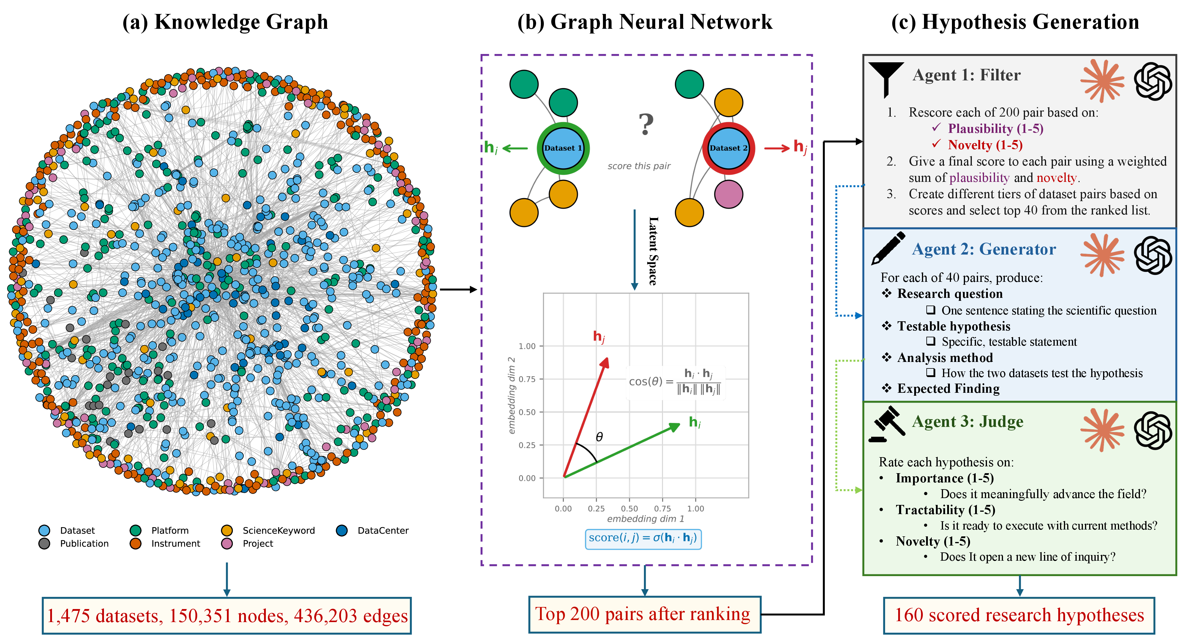
We therefore explore a complementary architecture in which the retrieval step itself is structured. We retrieve over a heterogeneous knowledge graph of EO research artifacts, where datasets, platforms, instruments, science keywords, and projects appear as typed nodes, and dataset co-usage (derived from joint citation by a shared publication), platform–instrument mounting, and dataset–metadata membership appear as typed edges. A heterogeneous graph neural network, trained by link prediction on past co-usages (publications through 2022), ranks candidate dataset pairings by predicted co-usage likelihood and surfaces the top 200 pairs not observed in the training, validation, or test co-usage sets. A three-agent LLM pipeline then refines this list: a filter agent rescores the top candidates on plausibility and novelty, a generator agent articulates a structured research hypothesis (question, testable claim, analysis method, expected finding) for each surviving pair, and a judge agent rates the resulting hypothesis on importance, tractability, and novelty under both blind and contextual conditions. 1 shows the complete pipeline.
Applied to the NASA Earth Observation Knowledge Graph, the pipeline produces 160 hypotheses spanning multiple Earth science domains. Held-out real co-usages and model-predicted novel pairings receive comparable plausibility scores from LLM judges, suggesting that the system surfaces scientifically coherent yet unexplored combinations. A representative example pairs IceBridge airborne magnetometer with InSAR-derived Antarctic ice velocity: the generator proposes that subglacial magnetic anomalies predict basal-friction patterns underlying modern ice flow—linking solid-Earth geology to cryospheric dynamics with public archives.
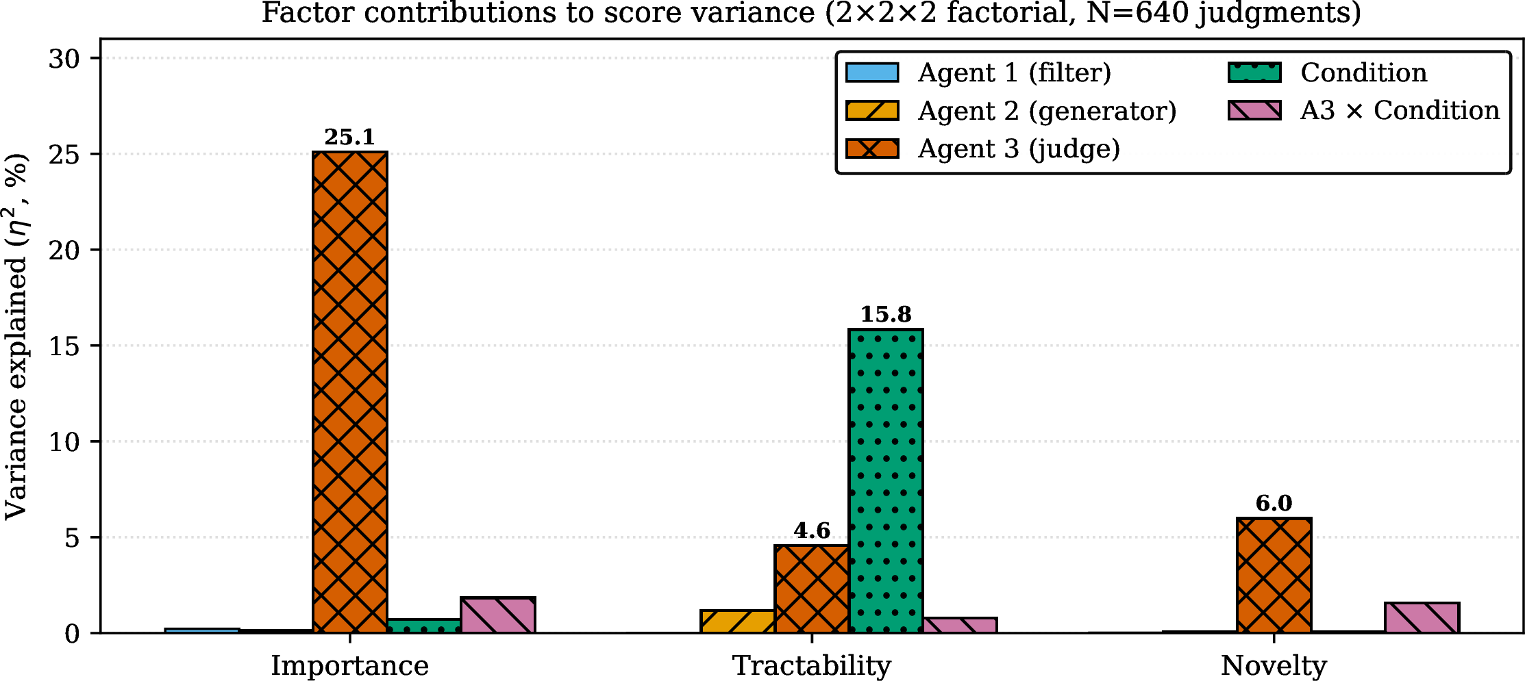
Because these scores can shift depending on which model plays which role, we test the pipeline under all eight combinations of GPT-5.2 and Claude Sonnet 4.6 across the three agent roles. These eight setups produce 640 judgments across the 160 hypotheses. We find that the ranking of hypotheses stays consistent (159 of 160 hypotheses change by at most 2 points across the four judge conditions), but the absolute scores depend heavily on which model is the judge: about \(25\%\) of the variation in importance scores comes from the judge alone, versus less than \(2\%\) from the filter or the generator. For tractability, the biggest factor is instead whether the judge sees the underlying datasets or only the hypothesis text (\(16\%\) of the variance). Together, these findings suggest that relying on a single LLM judge is risky for absolute scoring, and motivate the multi-judge protocol we use throughout the paper.
Our contributions are threefold:
We introduce a hypothesis-generation pipeline for observational science that ties each LLM-generated hypothesis to a specific pair of NASA datasets, surfaced by a knowledge-graph ranker rather than by free-form text retrieval, yielding 160 structured hypotheses across many Earth-science domains, with five flagship themes highlighted in 13.
We show that the pairs the model predicts as novel are rated nearly as plausible by LLM judges as held-out real co-usages from the published literature, which is evidence that the pipeline produces scientifically coherent ideas beyond what the model has already seen.
We run a \(2{\times}2{\times}2\) factorial over filter, generator, and judge identity and find that, although hypothesis rankings are stable across setups, the absolute scores depend strongly on which model is the judge—a warning about relying on a single LLM judge for this kind of evaluation. We release the knowledge-graph preprocessing, the trained GNN, all 160 hypotheses, the 640 validator judgments, and the full analysis code.
2 Related Work↩︎
2.0.0.1 LLM hypothesis generation from literature.
A growing line of work uses LLMs to generate research ideas grounded in text. Prior systems explore retrieval-based and multi-agent approaches for scientific ideation, including SciMON [3], ResearchAgent [9], MOOSE-Chem [1], and ResearchTown [10]. Fully autonomous pipelines [7], [8] further extend this to end-to-end ideation, experimentation, and manuscript writing, while large-scale expert studies [6] show that LLM-generated ideas can be judged more novel than human expert ideas, though often less feasible. All of this work retrieves over unstructured scientific text and treats a hypothesis as a free-form natural-language claim. In observational, data-rich domains such as Earth observation, the unit of discovery is instead a specific pair of measurement products whose joint analysis is executable, which motivates our GNN-over-typed-KG ranker (3) in place of literature retrieval.
2.0.0.2 Multi-agent and data-grounded discovery.
Closer to our setting, multi-agent pipelines ground generation in structured artifacts. SciAgents [4] reasons over an ontological knowledge graph with Ontologist, Scientist, and Critic roles for bioinspired materials; AstroAgents [5] generates astrobiology hypotheses from mass-spectrometry measurements with eight role-specialized agents; MOOSE-Chem2 [2] targets fine-grained hypotheses with concrete methodology via hierarchical search; AutoDiscovery [11] drives open-ended discovery across 21 real datasets with Bayesian surprise as an LLM-defined reward under Monte Carlo tree search. Our pipeline shares their role specialization and structure-grounded retrieval, but differs on two axes. First, retrieval operates on a typed, empirical dataset co-usage graph with a heterogeneous GNN ranker rather than per-query literature retrieval or symbolic ontology traversal, so every generated hypothesis is pinned to two named NASA products and is actionable by construction. Second, prior pipelines typically fix one LLM per role and —in the agentic case— equip that LLM with execution tools; we instead cross agent identity in a \(2{\times}2{\times}2\) factorial (5) and report the resulting variance decomposition, which is particularly consequential when the reward itself is LLM-defined, as in [3] and [11].
2.0.0.3 LLM-as-judge and evaluation reliability.
The reliability of LLM-based evaluation has been studied extensively. [12] introduce the LLM-as-judge formulation and document position, verbosity, and self-enhancement biases. [13] analyze scalable-oversight protocols in which weak LLM judges adjudicate strong LLM agents, identifying positional and order effects across nine reasoning asymmetries. [14] catalog twelve bias types and automate their quantification via CALM; [15] isolate self-preference bias and link it to perplexity, predicting that a judge will prefer outputs whose distribution is familiar to it. Most recently, [16] propose a plug-in Reasoning-based Bias Detector for post-hoc correction. Our factorial contributes an empirical variance decomposition in the scientific-hypothesis evaluation regime: judge identity accounts for roughly \(25\%\) of importance-score variance, dwarfing filter or generator effects (\({<}2\%\)), and the blind-versus-contextual contrast dominates tractability variance (\({\sim}16\%\)). This is precisely the failure mode anticipated by [15] and [14], and the one [16] aims to mitigate, now quantified in the hypothesis-evaluation setting for the first time.
2.0.0.4 Machine learning for Earth observation.
[17] argue that satellite data is a distinct ML modality and call for dedicated infrastructure. The dominant response has been to scale foundation models over individual imagery products [18]–[20], surveyed in [21]. At the community level, [22] articulate eleven desiderata for ideal Earth foundation models and explicitly flag cross-dataset knowledge synthesis as an open gap. Our work targets precisely that complementary discovery layer: given hundreds of heterogeneous NASA products, which pairings are worth a researcher’s time? We address this question here.
3 Knowledge Graph and GNN Retrieval↩︎
3.0.0.1 Knowledge graph.
We build on the publicly released NASA Earth Observation Knowledge Graph (EO-KG) [23]: a single GraphML resource with 150,351 nodes and
436,203 edges, spanning seven node types (Publication, Dataset, ScienceKeyword, Instrument, Platform, Project, DataCenter) and nine typed relations covering
citation, dataset usage, metadata membership, and a science-keyword subcategory hierarchy. The ranking universe consists of the 1,475 datasets that participate in at least one training-period co-usage pair (i.e., are co-cited with another dataset by at
least one paper with year \(\le 2022\)). This is by construction the natural evaluation pool for our link-prediction task and is also the candidate pool used for negative sampling during training. Per-type counts and the
full relation breakdown are in 9.
3.0.0.2 Deriving co-usage supervision.
The raw KG contains no direct dataset–dataset edge; we derive co-usage from Publication\(\to\)Dataset edges. For every publication \(p\) with dataset set \(D_p = \{d_{p,1}, \dots, d_{p,k}\}\), \(k \ge 2\), and every unordered pair \((d_i, d_j) \in D_p\), we emit a co-usage observation tagged with the publication
year. Pairs are labeled binary (co-used vs.not); multiplicity is retained as a weight only for auxiliary analyses. We then split pairs temporally by the publication year of each paper that observes them: train (\(\le
2022\)), val (\(=2023\)), test (\(=2024\)), giving 13,529 / 6,119 / 6,319 pairs. A pair co-cited in papers from multiple years enters multiple splits; we report test pairs unseen
in train (3,944) as the strict held-out subset used for evaluation. Within test we carve two harder subpools: cold-start (2,284 pairs, at least one endpoint with no training co-usage) and cross-DAAC (1,480 pairs, endpoints in
distinct archives). Full statistics are reported in 7.
3.0.0.3 Heterogeneous GNN ranker.
Let \(\mathcal{G}\) be the training graph induced by five surviving node types (Dataset, ScienceKeyword, Instrument, Platform, Project) and six typed
relations: co_usage between datasets, plus has_platform, has_keyword, has_instrument, of_project, and has_subcategory. Each Dataset node is initialized with a
768-dim SPECTER2 abstract embedding [24], [25]; non-dataset
types receive Xavier-initialized learnable embeddings of the same dimension. Publication nodes are removed from \(\mathcal{G}\): they served only to derive co-usage supervision, and retaining them would leak test pairs
through shared neighbors.
We learn \(d{=}128\) dimensional node representations with a two-layer heterogeneous GraphSAGE [26], [27]. Within each layer \(\ell\), for every typed relation \(r\) and every target node \(v\)
reachable through \(r\), we form a per-relation message \[\mathbf{m}_v^{(\ell+1,\,r)} \;=\; \mathbf{W}_r^{(\ell)} \, \mathrm{MEAN}_{u \in \mathcal{N}_r(v)}\, \mathbf{h}_u^{(\ell)},\] where
\(\mathcal{N}_r(v)\) are the neighbors of \(v\) under \(r\). Messages incoming to \(v\) are summed across all incident
relations and combined with the self-state through a SAGE residual, \[\mathbf{h}_v^{(\ell+1)} \;=\; \sigma\!\Big( \mathbf{W}_{\mathrm{self}}^{(\ell)} \mathbf{h}_v^{(\ell)} + \!\!\sum_{r \in \mathcal{R}_v}\!
\mathbf{m}_v^{(\ell+1,\,r)} \Big),\] where \(\mathcal{R}_v\) is the set of relations incident on \(v\), \(\sigma {=} \mathrm{ReLU}\), and dropout
\(0.2\) is applied to \(\mathbf{h}_v^{(\ell+1)}\). Per-relation weights \(\mathbf{W}_r^{(\ell)}\) are not shared across relations; this is what
distinguishes the heterogeneous variant from a homogeneous SAGE applied to the union graph and what allows the model to respect the feature-heterophilic structure inherent to typed graphs [28]. We use \(L{=}2\) layers; the (Dataset, co_usage, Dataset) relation participates in message passing on training pairs only.
The final dataset embeddings \(\mathbf{h}_i \!=\! \mathbf{h}_i^{(L)}\) are passed through one of two scorers, \[\begin{align} z_{\mathrm{dot}}(i, j) &= \mathbf{h}_i^{\!\top}\, \mathbf{h}_j, \\ z_{\mathrm{mlp}}(i, j) &= \operatorname{MLP}\!\big([\mathbf{h}_i \,\|\, \mathbf{h}_j]\big), \end{align}\] with the MLP being a two-layer network with hidden width \(d\) and ReLU activation. Both produce a logit; predicted co-usage probability is \(\sigma(z(i,j))\). We report both heads because, as we show below, they form a Pareto pair across the evaluation pools.
3.0.0.4 Training objective.
Stage 2 is trained by binary cross-entropy with logits. Each minibatch \(\mathcal{B}\) samples one training positive \((s, t^{+})\) together with one negative \((s, t^{-})\), and minimizes \[\mathcal{L}(\mathcal{B}) = -\sum_{(s,t^{+},t^{-}) \in \mathcal{B}} \Big[ \log \sigma(z(s,t^{+})) + \log\big(1 - \sigma(z(s,t^{-}))\big) \Big].\] Negatives are drawn from a degree-biased proposal, \(\Pr(t^{-} \!=\! n) \!\propto\! \deg(n)^{0.75}\) (matching the word2vec convention of upweighting hub candidates so that the ranker is forced to discriminate against plausible distractors), with rejection of any \(n\) that is itself a training positive of \(s\). Optimization uses Adam at learning rate \(10^{-3}\) for up to 300 epochs, with early stopping on validation MRR (patience 30).
3.0.0.5 Evaluation protocol.
We evaluate as a 1:100 ranking task: each held-out positive \((a, b^{+})\) is scored against 100 degree-matched negatives \(\{b^{-}_k\}_{k=1}^{100}\), and we report Hits@\(k\), mean reciprocal rank (MRR), AUC, and average precision (AP) on each of the three pools defined above. Hits@\(k\) is the fraction of held-out positives ranked in the top \(k\) over the 101-element candidate list; MRR is the mean of \(1/\mathrm{rank}(b^{+})\).
3.0.0.6 Baselines.
We compare against six baselines spanning structure-only and content-only signals. Popularity ranks candidates by global degree: \(z(i, j) = \deg(j)\), ignoring \(i\) entirely. Common Neighbors and Adamic–Adar score the candidate by overlap of co-usage neighborhoods, \(z(i, j) = \sum_{u \in \mathcal{N}(i) \cap \mathcal{N}(j)} \!w(u)\), with \(w \!\equiv\! 1\) for the former and \(w(u) \!=\! 1/\log|\mathcal{N}(u)|\) for the latter. MF-SVD factorizes the binary publication\(\times\)dataset co-citation matrix by truncated SVD (\(k=128\)) and scores pairs by inner product of the resulting dataset rows. SPECTER2 [24] and BGE-base [29] are dense-retrieval baselines that score pairs by cosine similarity of the corresponding dataset abstract embeddings, giving us a content-only ceiling to compare the GNN against.
| Method | All | Cold-start | Cross-DAAC |
|---|---|---|---|
| Popularity | 0.140 | 0.064 | 0.130 |
| MF-SVD | 0.192 | 0.274 | 0.125 |
| Common Neighbors | 0.349 | 0.211 | 0.228 |
| Adamic-Adar | 0.355 | 0.225 | 0.235 |
| BGE-base | 0.394 | 0.484 | 0.103 |
| SPECTER2 | 0.413 | 0.477 | 0.127 |
| GNN-Homo | 0.448 | 0.473 | 0.146 |
| GNN-Hetero (dot) | 0.468 | 0.519 | 0.175 |
| GNN-Hetero (MLP) | 0.467 | 0.389 | 0.266 |
4pt
3.0.0.7 Results.
1 reports Hits@10 across the three pools, and the cross-pool pattern is sharp. Popularity is essentially a prior on dataset frequency and accordingly performs near floor on all (0.140) and cold-start (0.064). The two co-usage-graph heuristics, Common Neighbors (0.349) and Adamic–Adar (0.355), more than double Popularity on all, but their reliance on observed neighbors is fatal on cold-start (0.211, 0.225), where at least one endpoint has no training neighborhood at all. MF-SVD shows the opposite asymmetry: its 128-dim factorization happens to generalize on cold-start (0.274) but loses on cross-DAAC (0.125), where bipartite co-citation structure does not constrain inter-archive pairs. Content baselines invert this picture again: SPECTER2 and BGE-base dominate cold-start (0.477 and 0.484), confirming that abstract semantics is the strongest single signal when no structural cue is available, but they collapse on cross-DAAC (0.127, 0.103). The intuition is that abstracts of cross-archive datasets share substantial Earth-science boilerplate, so cosine similarity ceases to discriminate plausible joint analyses from coincidental textual overlap.
The two GNN variants combine these signals. GNN-Homo matches the content baselines on cold-start (0.473) and exceeds them on all (0.448), but gains little on cross-DAAC (0.146). GNN-Hetero, which carries type-specific aggregators across the metadata relations, is the first method competitive on all three pools simultaneously: it improves cold-start to 0.519 and lifts cross-DAAC to 0.175. The two scorer heads form a clear Pareto pair: the dot-product head peaks on cold-start (0.519) while the MLP head peaks on cross-DAAC (0.266)—a substantial \(0.091\) absolute gain over its dot-product counterpart, attributable to the MLP’s ability to learn nonlinear combinations of the two embeddings that compensate for the type-confounded similarity between cross-archive datasets. We deploy the dot-product head as the retrieval feed to Agent 1 (selected by validation MRR over the all pool) and release both embedding sets with the code; the per-pool, per-metric breakdown for all configurations and the 11-lever ablation that selected this configuration are in 10.2 and 10.3.
4 Three-Agent LLM Pipeline↩︎
The 200 predicted-novel pairs surfaced by the GNN (3) are the input to a three-agent LLM cascade. Each agent has a distinct role: scoring, generation, and judgment. Each agent is independently instantiated with one of two backbones (GPT-5.2 or Claude Sonnet 4.6). All three agents return strictly JSON-formatted output with a fixed schema, queried at temperature \(0\) to remove sampling variance from the experiment. The full system prompts, user templates, and JSON schemas for all four roles (Agent 1, Agent 2, Agent 3 blind, Agent 3 contextual) are reproduced verbatim in 11.
4.0.0.1 Agent 1 — pair-level filter.
Agent 1 receives a candidate pair \((d_i, d_j)\) together with the two datasets’ short names, long names, and abstracts (truncated at 1,200 characters), and returns two integer scores on a \(1\)–\(5\) scale: plausibility (could a research team reasonably combine these datasets in a single study?) and novelty (how non-obvious is the combination?), plus a two-to-three sentence rationale. Scoring is deliberately decoupled from generation: Agent 1 sees no hypothesis text, so its rating reflects the pair itself, not how well a generator happens to motivate it. To anchor the scoring distribution and provide a positive control, Agent 1 is run not only on the 200 predicted-novel pairs (stratum A) but also on three additional strata of equal size containing held-out real co-usages sampled from 2024 publications, giving 800 scored pairs per Agent 1 backbone. Because the held-out pool is what the GNN was not trained on, comparing the plausibility distribution of stratum A against strata B–D is a direct test of whether predicted-novel pairs are scientifically coherent at the level of literature co-usages (6). For each Agent 1 backbone we select 40 pairs to forward to the generator, drawn exclusively from stratum A. We use a tiered rule rather than ranking by a single composite score, because plausibility and novelty answer different questions and naive scalarization would let either dimension dominate. Tier 1 takes pairs with maximal plausibility (\({=}5\)) and at least moderate novelty (\(\ge 3\)); tier 2 takes pairs with high plausibility (\(=4\)) and high novelty (\(\ge 4\)); tier 3 takes pairs with maximal plausibility (\(=5\)) and modest novelty (\(=2\)), which capture obvious-yet-strong pairings as a sanity floor. Within each tier, pairs are ordered by a weighted composite score, giving 55% weight to plausibility and 45% to novelty, and the top 40 are taken in order Tier 1 \(\to\) Tier 2 \(\to\) Tier 3, with a fallback to all \(\text{plaus} \ge 4\) pairs ranked by the same score if the three tiers yield fewer than 40.
4.0.0.2 Agent 2 — hypothesis generator.
Agent 2 receives one selected pair \((d_i, d_j)\) together with their short names, long names, and abstracts, and returns a structured research hypothesis with six fields: a one-sentence research question, a one-to-two sentence testable hypothesis, an analysis method describing how the two datasets jointly test it, an expected finding that would constitute support, a one-to-two sentence statement of scientific importance, and a one-to-three word domain tag. Critically, Agent 2 does not see Agent 1’s plausibility or novelty scores; this prevents the generator from regressing toward its own filter’s preferences and keeps generation a reflection of what the backbone independently considers worth proposing.
4.0.0.3 Agent 3 — judge under blind and contextual conditions.
Agent 3 evaluates each generated hypothesis on three integer scales: importance (does it meaningfully advance the field?), tractability (is it ready to execute with current methods?), and novelty (does it open a new line of inquiry?). Each hypothesis is judged twice—once blind (Agent 3 sees only the six hypothesis fields, with no information about which datasets underlie them) and once contextual (Agent 3 sees the hypothesis fields plus the underlying pair’s short names, long names, and abstracts). The blind/contextual contrast isolates how much of the judgment depends on the hypothesis text alone versus on inspectable evidence about the datasets. We will show in 6 that this contrast is the single largest source of variance in tractability scores, dwarfing both filter and generator effects.
5 Factorial Experiment↩︎
To diagnose how much each agent contributes to the quality scores the pipeline reports, we run the three-agent cascade (4) under all eight assignments of backbone to role in a \(2{\times}2{\times}2\) factorial design. The three factors are the identities of the filter (Agent 1), the generator (Agent 2), and the judge (Agent 3); each is independently set to either GPT-5.2 or Claude Sonnet 4.6. A fourth nested factor, judging condition, varies whether the judge sees the underlying dataset metadata (contextual) or only the hypothesis text (blind). All other components of the pipeline including the GNN ranker, the four-stratum input pool fed to Agent 1, the tiered top-40 selection, prompt templates, JSON schemas, and the temperature-\(0\) decoding are held constant across cells, so any observed differences are attributable to backbone identity or to the blind/contextual contrast.
5.0.0.1 Cells and counts.
The factorial yields four hypothesis sets indexed by \((a_1, a_2)\), each containing 40 hypotheses, for a total of 160 distinct hypotheses. Each hypothesis is then scored by both judge backbones \(a_3 \in \{\text{GPT}, \text{Claude}\}\) under both judging conditions, producing \(160 \times 4 = 640\) validator judgments. Each judgment returns three integer scores on a \(1\)–\(5\) scale (importance, tractability, novelty) plus a free-text rationale. Agent 1 itself is also a factorial cell with 800 inputs (4 strata of 200 pairs), giving \(2 \times 800 = 1{,}600\) Agent 1 ratings used both to feed the top-40 selection and to characterize how predicted- novel pairs (stratum A) compare against held-out real co-usages (stratum B) and two control strata (6).
5.0.0.2 Why factorial.
The dominant practice in LLM-as-scientist evaluations is to fix one backbone in each role and report the resulting scores as if they were properties of the hypotheses being judged. The factorial design instead lets us decompose score variance across the four nominal factors (filter, generator, judge, condition) and their two-way interactions using a standard one-way ANOVA per axis, reporting effect sizes as \(\eta^2\). This decomposition asks a direct question: when an importance score moves from 3 to 4, how much of that movement is signal about the hypothesis, and how much is the contingent identity of the backbones playing each role? We will show that for some axes the answer is uncomfortable.
6 Results↩︎
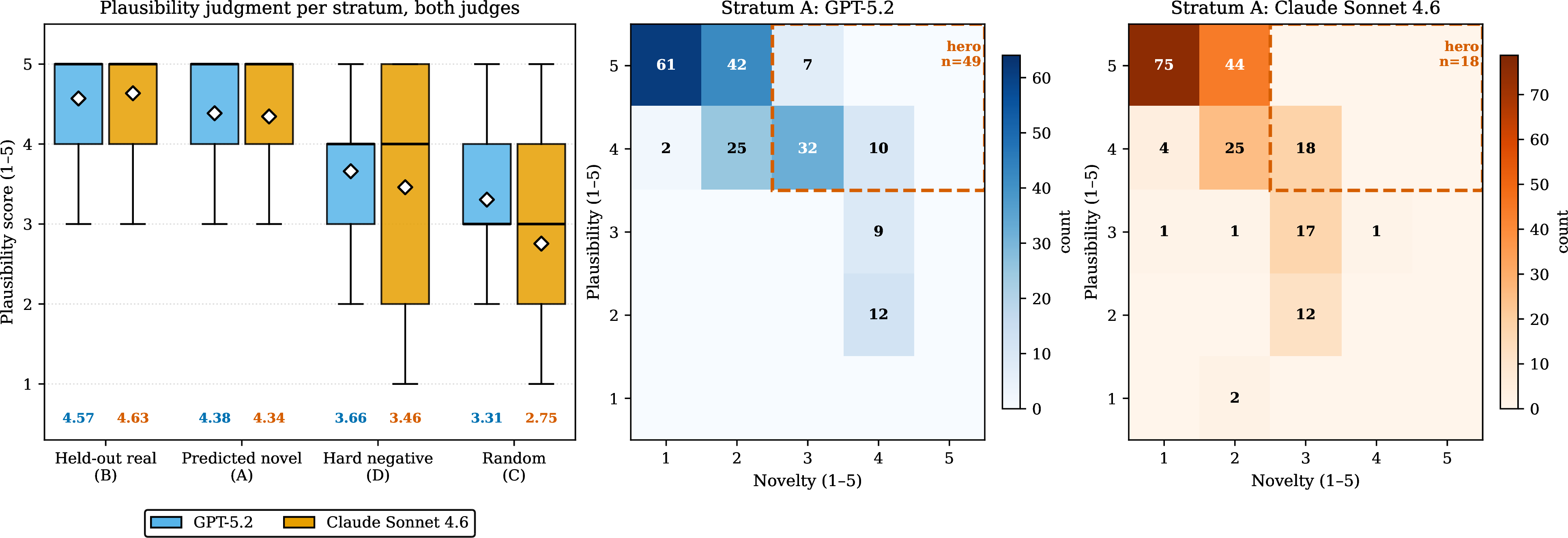
6.0.0.1 Stage 4: predicted-novel pairs are nearly as plausible as held-out real co-usages.
2 reports the Agent-1 stratum-level results and 2 visualizes the \((\text{plausibility}, \text{novelty})\) joint distribution for stratum A under each judge. Both judges order the four strata identically: held-out real 2024 co-usages (B) on top, GNN-predicted novel pairs (A) a hair below, then same-DAAC random “hard negatives” (D), and fully random pairs (C) at the bottom. Critically, the gap between A and B on plausibility is tiny—0.19 for GPT (4.38 vs.) and 0.29 for Claude (4.34 vs.)— while the gap between A and the random control C is more than five times larger (\(\ge\)1.07 for GPT, \(\ge\)1.59 for Claude). The GNN therefore surfaces predicted-novel pairs that LLM judges find essentially indistinguishable in scientific plausibility from pairs that were actually co-used in 2024 publications. The novelty axis, by contrast, fails to separate A from B: judges rate the predicted-novel pairs as no more novel than held-out real co-usages, a pattern we return to in 7 as a caution about LLM-as-novelty-judge. The joint distribution in 2 additionally exposes a calibration shift between judges: 49 of 200 stratum-A pairs land in GPT’s hero zone (plausibility \(\ge 4\) and novelty \(\ge 3\)), versus only 18 in Claude’s, reflecting a tighter Claude novelty distribution (2) rather than a difference in plausibility ranking. This calibration mismatch is the practical reason we run the tiered top-40 selection independently per Agent-1 backbone rather than pooling.
| Stratum | Plausibility | Novelty | ||
|---|---|---|---|---|
| 2-3(lr)4-5 | GPT-5.2 | Claude 4.6 | GPT-5.2 | Claude 4.6 |
| B | 4.57 | 4.63 | 2.35 | 1.86 |
| A | 4.38 | 4.34 | 2.19 | 1.84 |
| D | 3.66 | 3.46 | 3.17 | 2.48 |
| C | 3.31 | 2.75 | 3.52 | 2.75 |
4pt
6.0.0.2 Stage 5: variance decomposition.
3 reports the \(\eta^2\) contribution of each factor to score variance, by axis. Three patterns dominate. (i) Importance is a judge-identity question. Judge identity explains \(25.1\%\) of importance variance, while filter and generator identity together explain \(0.34\%\). In absolute terms the GPT judge rates importance roughly \(0.6\) points higher than the Claude judge in nearly every cell, regardless of who filtered or generated the hypothesis. (ii) Tractability is a context question. The blind/contextual contrast explains \(15.8\%\) of tractability variance versus \(4.6\%\) for judge identity; showing the dataset metadata reliably lowers tractability scores by about half a point (blind mean \(3.94\), contextual mean \(3.36\), averaged over the eight \((a_1,a_2,a_3)\) cells), suggesting that hypothesis text alone reads as more executable than it does once the actual measurement products are inspectable. (iii) Novelty is judge-dominated but small. Judge identity is again the largest single factor (\(6.0\%\)), but no factor explains more than \(\sim\)10% of variance on novelty—consistent with the Stage-4 finding that LLM judges do not strongly discriminate novelty across pair types. Filter and generator identity contribute essentially zero variance on every axis (\(\eta^2 < 0.013\) in all six cells), which has a useful corollary: Agent 1 and Agent 2 affect which hypotheses get scored, but their backbone identity does not bias the scores those hypotheses receive.
6.0.0.3 Inter-rater agreement: judges line up on tractability, diverge on importance.
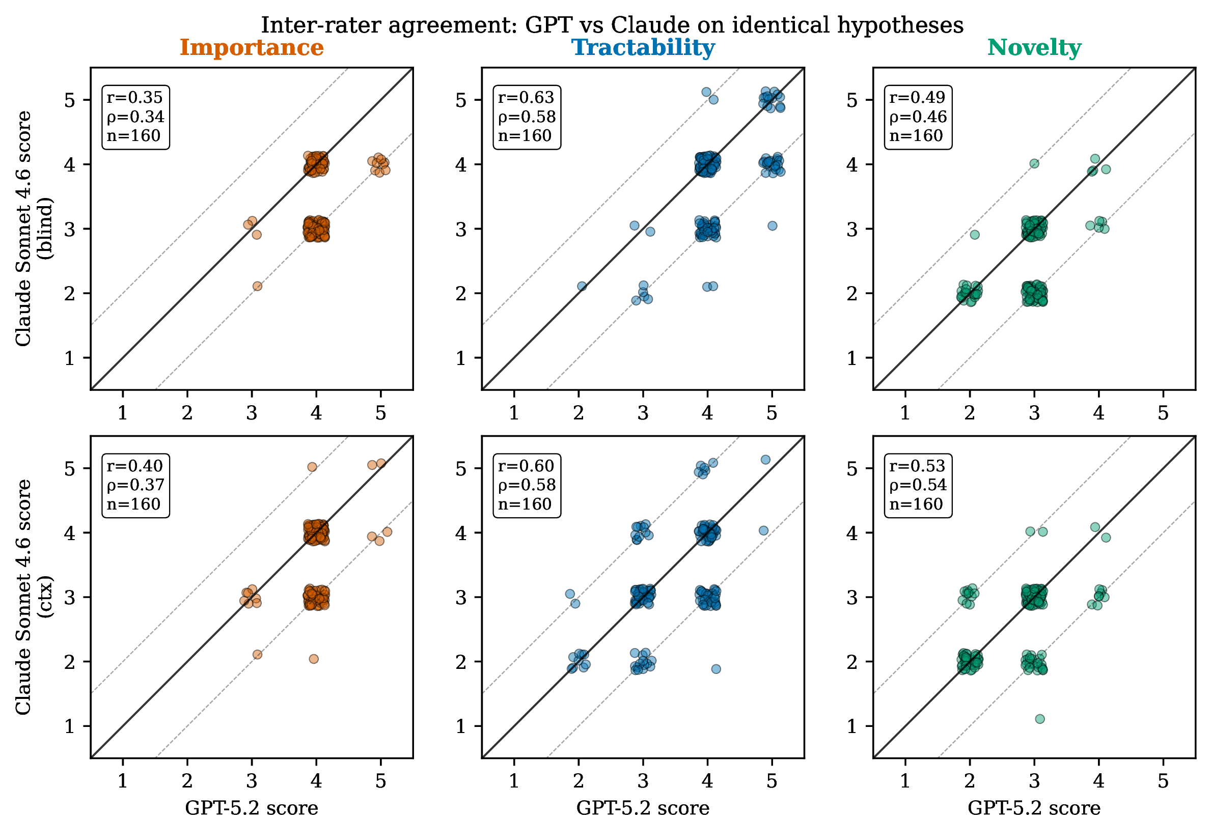
Inter-rater agreement between GPT-5.2 and Claude Sonnet 4.6 on identical hypotheses (full table in 12) is highest on tractability (Pearson \(r=0.63\) blind, quadratic-weighted \(\kappa_q=0.47\)), moderate on novelty (\(r=0.49\), \(\kappa_q=0.36\)), and weakest on importance (\(r=0.35\), \(\kappa_q=0.14\)). The ordering is the opposite of what one might expect—importance is arguably the most subjective of the three rubrics—but it is exactly what [15] predict for an LLM-as-judge setup: importance is the axis most coupled to a backbone’s training-time priors about what counts as “meaningful advance,” and consequently the axis on which two backbones with different pretraining mixtures disagree most. Showing dataset context improves agreement on all three axes, with the largest gain on importance (\(\kappa_q\): \(0.14 \to 0.24\), exact match: \(37\% \to 63\%\)), supporting the hypothesis that anchoring judges to inspectable evidence narrows the prior-driven disagreement.
6.0.0.4 Hypothesis ranking is stable across configurations.
The variance decomposition above is about the absolute scores, but for picking which hypotheses to actually pursue, what matters is the ranking—which hypothesis scores higher than which. That ranking turns out to be much more stable than the absolute scores. Across the four judge configurations (each pairing of judge backbone and blind/contextual condition), 159 of 160 hypotheses change by at most 2 points on every axis, with an average change of just \(1\) point. So even though one judge gives systematically higher scores than the other, the order in which they rank the hypotheses is nearly the same. A researcher who picks the top \(25\%\) by average score will get almost the same set no matter which single judge is used. The practical takeaway: single-judge scores are not portable in absolute terms, but the rankings they produce are reliable.
6.0.0.5 Flagship hypotheses.
A qualitative inspection of the highest-scoring outputs is deferred to 13, which lists five flagship hypotheses with the highest combined importance + tractability and a maximum cross- judge disagreement of one on every axis. The five span ecohydrology, glaciology, aerosol–cloud interactions, vegetation phenology, and methodological bias correction in cloud retrieval; all five are pinned to two named NASA products and are executable today with public archives—the deployment property the pipeline was designed to preserve.
7 Discussion and Limitations↩︎
7.0.0.1 Scope: ideation, not execution.
Our three agents operate text-only by design: filter and judge are evaluative roles where tool use buys little, and generator is an ideation role whose output is intended to seed human-led investigation rather than autonomously execute it. This scope choice has a second benefit specific to our methodology: the variance decomposition of 6 is interpretable precisely because every backbone receives identical inputs at temperature \(0\) with strict- JSON decoding. Adding tool access would inject retrieval and execution stochasticity that would confound the agent-identity signal we set out to measure. We view text-only ideation and tool-equipped execution as complementary layers of a future end-to-end discovery system, with our pipeline supplying the candidate hypotheses an executor would attempt. The most important limitation of this work is that the 160 hypotheses we report are LLM-judged, not human-verified. A small domain-expert study—even on the five flagship hypotheses—would sharpen the claim that the pipeline produces actionable research seeds rather than merely well-formed text. Three further limitations deserve mention. First, the GNN treats co-usage as a binary signal and discards multiplicity; an edge-weight-aware variant might sharpen the ranker but is not the bottleneck identified by our ablation (10.3). Second, abstracts are truncated at 1,200 characters before being shown to any agent, which can clip relevant detail for long-abstract products and may under-represent some pairings. Third, our factorial covers two backbones, two judging conditions, and three rubric axes; it does not control for prompt phrasing, position bias within the user template, or temperature, all of which prior work has shown to move LLM-judge outputs [12], [14]. Quantifying their interaction with the variance budget reported here is a natural next step.
8 Conclusion↩︎
Hypothesis generation in observational sciences is a different problem from generation in literature-driven ones: the unit of discovery is a specific pair of measurement products, not a sentence. We addressed this by combining a heterogeneous GNN ranker over the NASA Earth-Observation Knowledge Graph with a three-agent LLM cascade, producing 160 structured, dataset-grounded research hypotheses spanning many Earth-science domains. Predicted- novel pairs are rated essentially as plausible as held-out real co-usages, and a \(2{\times}2{\times}2\) factorial over agent identity shows that hypothesis rankings are stable across LLM backbones while absolute scores are not—an empirical bound on what single-judge LLM-as-scientist evaluations can claim. We release the trained GNN, the 160 hypotheses, the 640 validator judgments, and the full pipeline as a reproducible substrate for both the EO community and the broader study of LLM-driven scientific discovery.
Impact Statement↩︎
This paper presents a system that suggests candidate research directions in Earth science; generated hypotheses are not scientific claims but seeds for human investigation, and each must be verified with domain experts and actual data analysis before being treated as a finding. We see no societal consequences requiring specific discussion beyond standard concerns about the use of LLM outputs in scientific contexts.
LLM Usage Disclosure↩︎
GPT-5.2 and Claude Sonnet 4.6 were used as pipeline components: they are the Agents 1, 2, and 3 described in 4, and their outputs are the experimental data reported in 6. In addition, Claude was used as a writing collaborator during drafting of this manuscript; all final wording and technical claims were verified by the authors.
9 Knowledge Graph Characterization↩︎
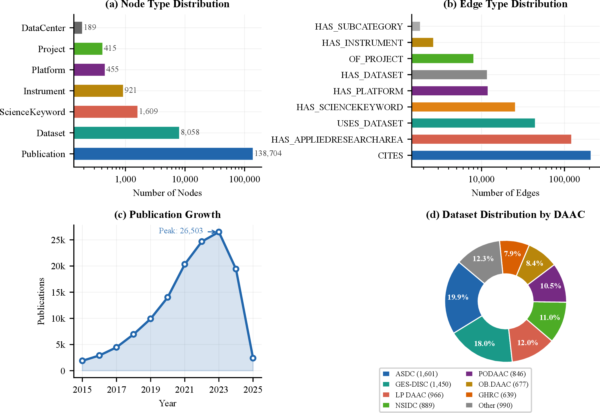
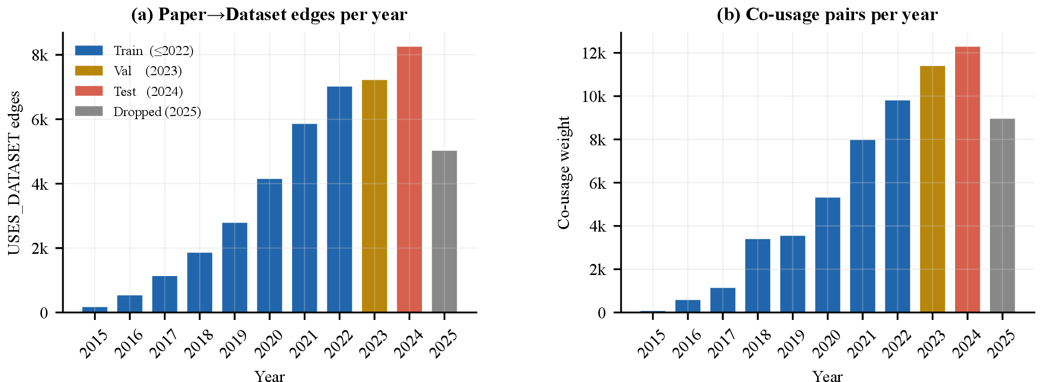
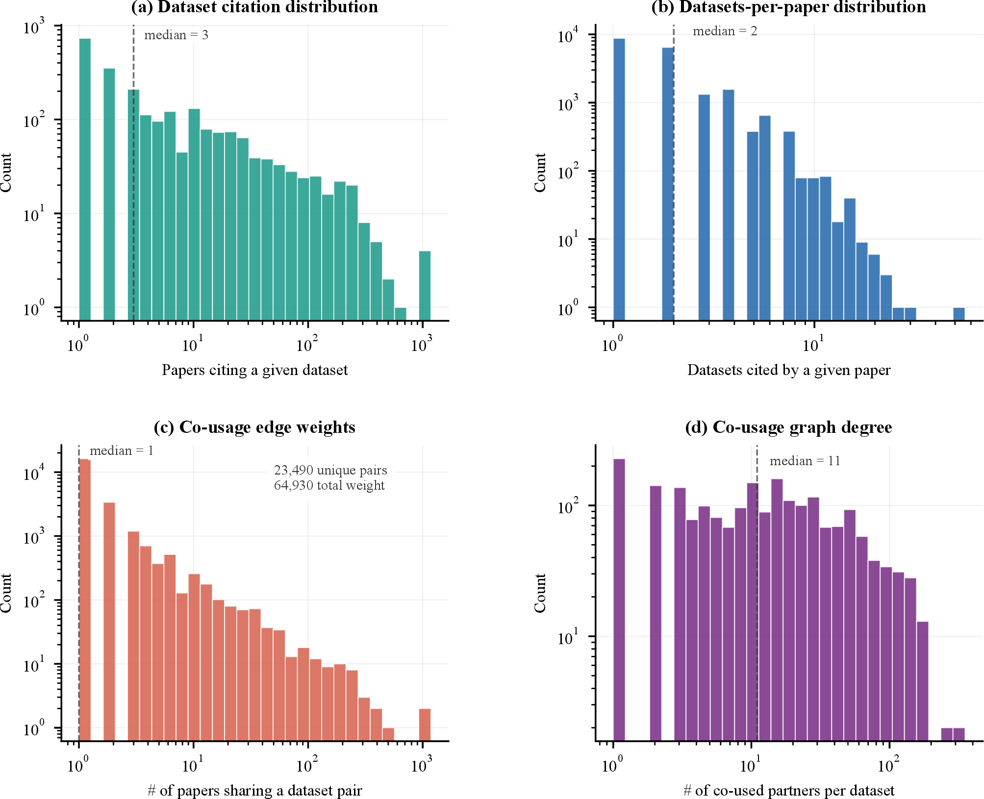
This appendix reports the full statistics of the NASA EO Knowledge Graph [23] summarized in 3. 3 lists global graph properties, 4 the seven node types, 5 the nine relation types, and 6 the dataset distribution across NASA’s Distributed Active Archive Centers, and 7 the derived co-usage statistics and temporal split sizes. 4 visualizes node- and edge-type distributions; 6 reports the citation and co-usage degree distributions; 5 shows the temporal split over publication year used for train/val/test.
| Property | Value | Note |
|---|---|---|
| Total nodes | 150351 | 7 distinct types |
| Total edges | 436203 | 9 relation types |
| Mean degree | 5.80 | Across all nodes |
| Publications | 138704 | 99.5% with title/abstract |
| Datasets | 8058 | 100% with CMR metadata |
| Dataset temporal span | 1972–2026 | Earliest start – latest end |
| CITES edges | 208616 | Citation network |
| USES_DATASET edges | 44354 | Publication \(\to\) Dataset |
| Node Type | Count | % | Key Attributes |
|---|---|---|---|
| Publication | 138704 | 92.3% | doi, title, year, authors, abstract |
| Dataset | 8058 | 5.4% | shortName, longName, daac, cmrId, temporal extent |
| ScienceKeyword | 1609 | 1.1% | name, subcategory hierarchy |
| Instrument | 921 | 0.6% | shortName, longName |
| Platform | 455 | 0.3% | shortName, longName, type |
| Project | 415 | 0.3% | shortName, longName |
| DataCenter | 189 | 0.1% | shortName, longName, url |
| Total | 150351 | 100% |
| Relation | Source | Target | Count | % |
|---|---|---|---|---|
| CITES | Publication | Publication | 208616 | 47.8% |
| HAS_APPLIEDRESEARCHAREA | Publication | ScienceKeyword | 121553 | 27.9% |
| USES_DATASET | Publication | Dataset | 44354 | 10.2% |
| HAS_SCIENCEKEYWORD | Dataset | ScienceKeyword | 25553 | 5.9% |
| HAS_PLATFORM | Dataset | Platform | 11944 | 2.7% |
| HAS_DATASET | DataCenter | Dataset | 11698 | 2.7% |
| OF_PROJECT | Dataset | Project | 8031 | 1.8% |
| HAS_INSTRUMENT | Platform | Instrument | 2631 | 0.6% |
| HAS_SUBCATEGORY | ScienceKeyword | ScienceKeyword | 1823 | 0.4% |
| Total | 436203 | 100% |
| DAAC | Full Name | Datasets | % |
|---|---|---|---|
| ASDC | Atmospheric Science Data Center | 1601 | 19.9% |
| GES-DISC | Goddard Earth Sciences DISC | 1450 | 18.0% |
| LP DAAC | Land Processes DAAC | 966 | 12.0% |
| NSIDC | Natl.Snow and Ice Data Center | 889 | 11.0% |
| PODAAC | Physical Oceanography DAAC | 846 | 10.5% |
| OB.DAAC | Ocean Biology DAAC | 677 | 8.4% |
| GHRC | Global Hydrology Resource Ctr. | 639 | 7.9% |
| Other | Remaining DAACs | 990 | 12.3% |
| Total | 8058 | 100% |
9.0.0.1 Why heavy-tails matter for Stage 2.
Panels (a)–(d) of 6 all exhibit heavy tails spanning two to three orders of magnitude. This imbalance is the practical reason we sample training negatives from \(\Pr(n) \propto \deg(n)^{0.75}\) rather than uniformly (3): uniform negatives would rarely include hub datasets, yet hubs are exactly where the ranking problem is hardest because they have many plausible partners. The edge-weight panel (c) additionally motivates our binary treatment of co-usage: weighting positives by the number of co-citing papers would upweight already-well-known pairings at the expense of the rarer, less well-traveled pairs that carry the most discovery value.
9.0.0.2 Why a temporal split.
A random held-out split would let the model see co-usages it will be evaluated on through common-neighbor paths (e.g., if pair \((A, B)\) is held out but papers citing \(\{A, B, C\}\) remain in train, the training signal leaks through \(C\)). The temporal split used here mitigates this leakage by partitioning pairs by the year of each observing paper, and the strictly held-out evaluation subset is the 3,944 test pairs that never appear in any training-era paper. This mirrors the deployment scenario the system is designed for, where the model must rank candidate pairings that the research community has not yet explored.
| Property | Value |
|---|---|
| Paper\(\to\)Dataset edges (total) | 44354 |
| Unique datasets cited | 2357 |
| Datasets with \(\ge 5\) papers | 949 |
| Papers citing \(\ge 2\) datasets | 11087 |
| Co-usage graph nodes | 2088 |
| Co-usage graph edges (unique pairs) | 23490 |
| Sum of co-usage weights | 64930 |
| Max pair weight | 1051 |
| Median / Max degree | 11 / 314 |
| Train co-usage pairs | 13529 |
| Val co-usage pairs | 6119 |
| Test co-usage pairs | 6319 |
| Test pairs unseen in train | 3944 |
| Cold-start test pairs | 2284 |
| Cross-DAAC test pairs | 1480 |
| Cross-instrument test pairs | 902 |
4pt
10 GNN Details, Full Baselines, and Ablation↩︎
10.1 Hyperparameters↩︎
Table 8 summarizes the full set of GNN hyperparameters. They were not tuned per pool; the same configuration is used for all three test pools.
| Hyperparameter | Value |
|---|---|
| Encoder | 2-layer heterogeneous GraphSAGE |
| Hidden dimension | 128 |
| Dropout | 0.2 |
| Dataset node features | SPECTER2, 768-dim (frozen) |
| Non-dataset node features | Xavier-initialized learnable |
| Optimizer | Adam |
| Learning rate | \(1 \times 10^{-3}\) |
| Max epochs | 300 |
| Early-stopping patience | 30 (on val MRR) |
| Negatives per positive (train) | 1 |
| Negative sampling distribution | degree\({}^{0.75}\) (rejection of training positives) |
| Loss | Binary cross-entropy with logits |
| Scorers | \(\sigma(\mathbf{h}_i \!\cdot\! \mathbf{h}_j)\) or \(\sigma(\mathrm{MLP}([\mathbf{h}_i; \mathbf{h}_j]))\) |
| Seeds | \(\{0, 1, 2\}\) |
10.2 Full baseline metrics↩︎
3 reports Hits@10 for compactness. 9 reports all five metrics (Hits@10, Hits@50, MRR, AUC, AP) for the six Stage-1 baselines on each of the three test pools; 10 reports the same for GNN-Homo and GNN-Hetero with mean \(\pm\) std over three seeds.
| Pool | Baseline | Hits@10 | Hits@50 | MRR | AUC | AP |
|---|---|---|---|---|---|---|
| all | Popularity | 0.140 | 0.562 | 0.070 | 0.542 | 0.012 |
| CommonNeighbors | 0.349 | 0.768 | 0.183 | 0.687 | 0.034 | |
| AdamicAdar | 0.355 | 0.763 | 0.190 | 0.691 | 0.035 | |
| MF-SVD | 0.192 | 0.433 | 0.101 | 0.491 | 0.022 | |
| SPECTER2 | 0.413 | 0.832 | 0.215 | 0.744 | 0.040 | |
| BGE-base | 0.394 | 0.802 | 0.210 | 0.727 | 0.038 | |
| cold_start | Popularity | 0.064 | 0.297 | 0.035 | 0.371 | 0.007 |
| CommonNeighbors | 0.211 | 0.566 | 0.123 | 0.557 | 0.011 | |
| AdamicAdar | 0.225 | 0.576 | 0.125 | 0.562 | 0.011 | |
| MF-SVD | 0.274 | 0.503 | 0.136 | 0.538 | 0.033 | |
| SPECTER2 | 0.477 | 0.847 | 0.270 | 0.761 | 0.054 | |
| BGE-base | 0.484 | 0.838 | 0.272 | 0.765 | 0.051 | |
| cross_daac | Popularity | 0.130 | 0.602 | 0.070 | 0.560 | 0.013 |
| CommonNeighbors | 0.228 | 0.701 | 0.122 | 0.630 | 0.018 | |
| AdamicAdar | 0.235 | 0.701 | 0.128 | 0.632 | 0.019 | |
| MF-SVD | 0.125 | 0.455 | 0.068 | 0.494 | 0.013 | |
| SPECTER2 | 0.127 | 0.683 | 0.063 | 0.605 | 0.012 | |
| BGE-base | 0.103 | 0.604 | 0.053 | 0.566 | 0.011 |
| Variant | Pool | H@10 | H@50 | MRR | AUC | AP |
|---|---|---|---|---|---|---|
| GNN-Homo | all | \(0.448\pm0.001\) | \(0.805\pm0.004\) | \(0.228\pm0.005\) | \(0.756\pm0.003\) | \(0.042\pm0.001\) |
| GNN-Homo | cold_start | \(0.473\pm0.005\) | \(0.808\pm0.006\) | \(0.240\pm0.013\) | \(0.758\pm0.006\) | \(0.034\pm0.002\) |
| GNN-Homo | cross_daac | \(0.146\pm0.001\) | \(0.594\pm0.008\) | \(0.072\pm0.002\) | \(0.574\pm0.004\) | \(0.012\pm0.000\) |
| GNN-Hetero | all | \(0.468\pm0.003\) | \(0.850\pm0.003\) | \(0.225\pm0.004\) | \(0.780\pm0.003\) | \(0.040\pm0.001\) |
| GNN-Hetero | cold_start | \(0.519\pm0.003\) | \(0.858\pm0.009\) | \(0.257\pm0.004\) | \(0.796\pm0.004\) | \(0.040\pm0.001\) |
| GNN-Hetero | cross_daac | \(0.175\pm0.006\) | \(0.669\pm0.005\) | \(0.077\pm0.003\) | \(0.615\pm0.004\) | \(0.014\pm0.000\) |
3pt
10.3 Cumulative ablation↩︎
11 reports our 11-lever cumulative ablation over both the homogeneous and heterogeneous GNN. Each row adds one lever on top of all previously kept levers; a lever is kept (\(✔\)) if its addition improves mean validation MRR by more than \(10^{-3}\) over the current best, with the sole exception that the first lever in each block (+pubs_uses for hetero,
+3_layers for homo) is retained as the chain’s starting point because the imported Stage-2 baseline carries no validation-MRR record to compare against, so its checkmark does not indicate an improvement. Three observations follow. First, the
heterogeneous baseline already dominates the homogeneous one on all three test pools, isolating the value of type-specific message passing. Second, after restricting publication nodes to year \(\le 2022\) to prevent
test-co-usage leakage through 2-hop message-passing paths, adding publication-derived edges (+pubs_uses, +pubs_area) yields no statistically meaningful improvement over the base heterogeneous architecture:
+pubs_area’s validation-MRR delta of \(+0.0009\) falls below our keep threshold (\(+10^{-3}\)), and Hits@10 on cold-start and cross-DAAC are slightly lower with
publications than without. Third, the dot-product and MLP scorer heads form a Pareto pair on cold-start versus cross-DAAC performance rather than a strict ordering: dot wins cold-start (0.519) by a substantial margin, MLP wins cross-DAAC (0.266) by an even
larger one, and the two are within \(0.001\) of each other on the all pool. We therefore release both embedding sets with the code so that downstream applications can pick the head that matches their target
distribution.
| Variant | Config | all | cold_start | cross_daac |
|---|---|---|---|---|
| homo | baseline \(✔\) | 0.448\(\pm\)0.001 | 0.473\(\pm\)0.005 | 0.146\(\pm\)0.001 |
| +3_layers \(✔\) | 0.418\(\pm\)0.007 | 0.418\(\pm\)0.014 | 0.150\(\pm\)0.019 | |
| +residual \(✔\) | 0.450\(\pm\)0.007 | 0.476\(\pm\)0.009 | 0.151\(\pm\)0.009 | |
| +layer_concat \(✔\) | 0.449\(\pm\)0.007 | 0.489\(\pm\)0.007 | 0.150\(\pm\)0.010 | |
| +neg_5x \(✔\) | 0.459\(\pm\)0.014 | 0.489\(\pm\)0.011 | 0.149\(\pm\)0.011 | |
| +bpr_loss | 0.439\(\pm\)0.004 | 0.476\(\pm\)0.006 | 0.138\(\pm\)0.005 | |
| +mlp_scorer | 0.266\(\pm\)0.001 | 0.133\(\pm\)0.005 | 0.198\(\pm\)0.002 | |
| +ensemble \(✔\) | 0.466\(\pm\)0.006 | 0.475\(\pm\)0.025 | 0.158\(\pm\)0.013 | |
| hetero | baseline \(✔\) | 0.468\(\pm\)0.003 | 0.519\(\pm\)0.003 | 0.175\(\pm\)0.006 |
| +pubs_uses \(✔\) | 0.467\(\pm\)0.003 | 0.513\(\pm\)0.011 | 0.171\(\pm\)0.014 | |
| +pubs_cites | 0.458\(\pm\)0.005 | 0.509\(\pm\)0.017 | 0.163\(\pm\)0.009 | |
| +pubs_area | 0.473\(\pm\)0.008 | 0.516\(\pm\)0.009 | 0.170\(\pm\)0.011 | |
| +edge_weights | 0.467\(\pm\)0.003 | 0.513\(\pm\)0.011 | 0.171\(\pm\)0.014 | |
| +3_layers | 0.452\(\pm\)0.007 | 0.511\(\pm\)0.009 | 0.155\(\pm\)0.016 | |
| +residual | 0.462\(\pm\)0.003 | 0.500\(\pm\)0.018 | 0.173\(\pm\)0.005 | |
| +layer_concat | 0.464\(\pm\)0.002 | 0.515\(\pm\)0.007 | 0.165\(\pm\)0.004 | |
| +neg_5x | 0.469\(\pm\)0.005 | 0.497\(\pm\)0.003 | 0.192\(\pm\)0.012 | |
| +bpr_loss \(✔\) | 0.465\(\pm\)0.002 | 0.508\(\pm\)0.007 | 0.170\(\pm\)0.013 | |
| +mlp_scorer \(✔\) | 0.467\(\pm\)0.005 | 0.389\(\pm\)0.006 | 0.266\(\pm\)0.011 | |
| +ensemble \(✔\) | 0.470\(\pm\)0.008 | 0.377\(\pm\)0.014 | 0.271\(\pm\)0.017 |
11 Three-Agent Prompts and JSON Schemas↩︎
The four colored boxes below reproduce verbatim the system prompts, user-message templates, and JSON output schemas used in the three-agent pipeline of 4. The same prompts are used regardless of which backbone
(GPT-5.2 or Claude Sonnet 4.6) is playing the role, so that any difference in the resulting scores reflects the backbone, not the prompt. All four call sites use temperature \(0\) and the API’s strict-JSON response format
(GPT: response_format=json_object; Claude: defensive post-hoc fence stripping).
Backbone: GPT-5.2 or Claude Sonnet 4.6. Temperature: \(0\). Max output tokens: 400.
System prompt
You are an expert Earth-science research scientist. Your job is to evaluate whether two Earth-observation datasets could plausibly be combined in a single scientific study. Base your judgment on the datasets’ scientific content as described in their abstracts, not on whether you have seen them combined before in published work. Respond with JSON only, in the exact schema requested.
User-message template
Please evaluate the following pair of Earth-observation datasets.
Dataset A:
Short name: {sn_a}
Long name:{ln_a}
Abstract:{abs_a}
Dataset B:
Short name: {sn_b}
Long name:{ln_b}
Abstract:{abs_b}
Rate this pairing on two axes:
1. SCIENTIFIC PLAUSIBILITY (1–5): Could a research team reasonably
combine these datasets in a single scientific study?
2. NOVELTY (1–5): How novel or non-obvious is this combination?
Output JSON schema
{ "plausibility": <1–5 int>,
"novelty":,
"rationale":"<2–3 sentence explanation>" }
Inputs: shortName, longName, and abstract (truncated to 1,200 characters) for each dataset. Output: two integer scores plus a free-text rationale.
Backbone: GPT-5.2 or Claude Sonnet 4.6. Temperature: \(0\). Max output tokens: 900.
System prompt
You are an expert Earth-observation research scientist. You will be given two NASA datasets. Generate ONE concrete, publishable research hypothesis that could be tested by combining them. Focus on scientific content, not data-availability caveats. Respond with JSON only.
User-message template
Dataset A:
Short name: {sn_a}
Long name:{ln_a}
Abstract:{abs_a}
Dataset B:
Short name: {sn_b}
Long name:{ln_b}
Abstract:{abs_b}
Generate one specific, testable research hypothesis that combines
these two datasets. The hypothesis must be concrete enough that a
team could plan an actual study, not a vague “one could investigate
X” statement.
Output JSON schema
{ "research_question":"<one-sentence question>",
"hypothesis":"<testable hypothesis, 1–2 sent.>",
"analysis_method":"<how datasets test it, 1–2 sent.>",
"expected_finding":"<what would support, 1 sent.>",
"scientific_importance": "<why it matters, 1–2 sent.>",
"domain":"<primary domain, 1–3 words>" }
Inputs: the surviving pair \((d_i, d_j)\) from the tiered top-40 selection, with the same dataset metadata Agent 1 received. Crucially, Agent 2 does not see Agent 1’s scores. Output: a six-field structured hypothesis.
Backbone: GPT-5.2 or Claude Sonnet 4.6. Temperature: \(0\). Max output tokens: 500.
System prompt
You are a senior Earth-observation research scientist reviewing a proposed research hypothesis. Judge the hypothesis on its scientific merit alone; you do not need to verify data availability. Respond with JSON only.
User-message template
Here is a proposed Earth-science research hypothesis:
Research question:{research_question}
Hypothesis:{hypothesis}
Proposed method:{analysis_method}
Expected finding:{expected_finding}
Scientific importance: {scientific_importance}
Domain:{domain}
Rate 1–5:
IMPORTANCE: = trivial, = meaningfully advances field
TRACTABILITY: 1 = needs breakthroughs, = ready to execute
NOVELTY: = already well-studied, = opens new line
Output JSON schema
{ "importance":,"tractability": <1–5>,
"novelty":,"rationale":"<2–3 sentences>" }
Inputs: only the six hypothesis fields produced by Agent 2; no dataset metadata. Output: three integer scores plus rationale.
Backbone: GPT-5.2 or Claude Sonnet 4.6. Temperature: \(0\). Max output tokens: 500.
System prompt
You are a senior Earth-observation research scientist reviewing a proposed research hypothesis along with the datasets it uses. Judge the hypothesis on scientific merit and the appropriateness of the dataset combination. Respond with JSON only.
User-message template
Dataset A:
Short name: {sn_a}
Long name:{ln_a}
Abstract:{abs_a}
Dataset B:
Short name: {sn_b}
Long name:{ln_b}
Abstract:{abs_b}
Proposed research hypothesis:
Research question:{research_question}
Hypothesis:{hypothesis}
Proposed method:{analysis_method}
Expected finding:{expected_finding}
Scientific importance: {scientific_importance}
Domain:{domain}
Rate 1–5 (same scales as the blind condition).
Output JSON schema
{ "importance":,"tractability": <1–5>,
"novelty":,"rationale":"<2–3 sentences>" }
Inputs: the same six hypothesis fields as the blind judge, plus the underlying pair’s shortName, longName, and abstracts (truncated to 1,200 characters). Output: three integer scores
plus rationale.
12 Factorial Design: Extended Analyses↩︎
This appendix presents three extended views of the Stage-5 factorial results summarized in 6.
12.0.0.1 Inter-rater agreement (Table 12).
12 reports the full inter-rater statistics referenced in 6: Pearson \(r\), Spearman \(\rho\), Cohen’s quadratic-weighted \(\kappa_q\), and the exact-match percentage between GPT-5.2 and Claude Sonnet 4.6 on identical hypotheses, separated by judging condition. The headline ordering holds for every metric (tractability \(>\) novelty \(>\) importance under both conditions), and the contextual-condition gain on importance (\(\kappa_q\): \(0.14 \to 0.24\), exact match: \(37\% \to 63\%\)) is the largest single improvement in the table.
| Axis | Cond. | \(n\) | Pearson \(r\) | Spearman \(\rho\) | \(\kappa_q\) | Exact % |
|---|---|---|---|---|---|---|
| Importance | blind | 160 | +0.351 | +0.337 | +0.137 | 37 |
| Importance | ctx | 160 | +0.397 | +0.366 | +0.241 | 63 |
| Tractability | blind | 160 | +0.627 | +0.578 | +0.472 | 54 |
| Tractability | ctx | 160 | +0.601 | +0.585 | +0.572 | 58 |
| Novelty | blind | 160 | +0.487 | +0.456 | +0.356 | 57 |
| Novelty | ctx | 160 | +0.527 | +0.541 | +0.512 | 71 |
4pt
12.0.0.2 Per-cell mean scores (Figure 7).
Three heatmaps report the mean validator score for every cell of the \(2{\times}2{\times}2\) factorial, with the blind/contextual condition appearing as adjacent column-pairs. Rows are \((a_1, a_2)\) filter–generator combinations; columns are \((a_3, \text{condition})\). The visual signature of the variance decomposition (3) is immediately visible: importance (left panel) splits cleanly by judge— the two GPT-judge columns are uniformly darker than the two Claude- judge columns regardless of \((a_1, a_2)\), with mean shifts of \(\sim 0.5\)–\(0.7\) points; tractability (middle panel) splits by condition—blind columns are uniformly darker than ctx columns within each judge; novelty (right panel) is mostly flat, consistent with its low total variance. The white vertical divider separates GPT-judge from Claude-judge columns; the dashed horizontal divider separates GPT-filter from Claude-filter rows.
![Figure 7: Per-cell mean validator score for each axis (importance, tractability, novelty). Rows: (a_1, a_2) filter–generator combinations. Columns: (a_3, \text{condition}) judge–condition combinations. Color scale uses the cividis colormap on the score range [2.0, 5.0]. The vertical white divider separates the GPT and Claude judges; the horizontal dashed divider separates GPT and Claude filters.](/article/2607.01584/figures/fig_factorial_heatmap.png "fig:")
12.0.0.3 Inter-rater scatter (Figure 8).
For every hypothesis judged under both backbones in the same condition, the scatter plots GPT’s score (x-axis) against Claude’s score (y-axis), with jitter added to separate ties. The diagonal is perfect agreement; the dashed diagonals mark \(\pm 1\) tolerance. Each panel reports Pearson \(r\) and Spearman \(\rho\) over its 160-point sample. The visualization makes the pattern from 12 concrete: tractability scatter clusters tightly around the diagonal under both conditions; novelty scatter is moderately tight; importance scatter exhibits a visible vertical bias (GPT systematically high) that narrows but does not vanish in the contextual condition.
13 Flagship Hypotheses↩︎
This appendix lists the five flagship hypotheses referenced in 6. Selection criterion: the highest combined importance + tractability scores with a maximum cross-judge disagreement of one on every axis, i.e., consensus high quality across all four judge conditions (\(a_3 \!\in\! \{\text{GPT}, \text{Claude}\} \!\times\! \{\text{blind}, \text{contextual}\}\)). The score columns Imp, Tract, and Novel report the mean across those four judgments; Max \(\Delta\) is the largest disagreement on any axis.
| Dataset pair | Domain | Imp | Tract | Novel | Max \(\Delta\) | Source (A1→A2) | Research question (abbreviated) |
|---|---|---|---|---|---|---|---|
| SPL4SMGP + MYD13Q1 | Ecohydrology | 4.00 | 4.50 | 3.00 | 1 | Claude\(\to\)GPT | Does sub-seasonal root-zone soil moisture variability control the timing and magnitude of vegetation greeni… |
| IRKUB1B + IRMCR1B | glaciology | 4.50 | 3.75 | 3.25 | 1 | GPT\(\to\)GPT | Do along-track changes in Ku-band surface echo strength predict the presence and thickness of near-surface… |
| MOD08_M3 + CAL_LID_L3_Tropospheric_APro_CloudFree-Standard-V4-20 | Aerosol-cloud | 4.50 | 3.50 | 3.25 | 1 | Claude\(\to\)GPT | Does the vertical placement of tropospheric aerosol (near-surface vs elevated layers) modulate the monthly… |
| MYD13A2 + MYD15A2H | vegetation phenology | 4.00 | 4.25 | 3.00 | 1 | GPT\(\to\)GPT | Does the seasonal relationship between canopy greenness (EVI/NDVI) and canopy structure (LAI/FPAR) exhibit… |
| MOD06_L2 + CAL_LID_L2_VFM-Standard-V4-20 | Cloud remote sensing | 4.00 | 4.75 | 2.50 | 1 | GPT\(\to\)GPT | Do MODIS/Terra MOD06_L2 cloud optical thickness and effective radius retrievals exhibit systematic biases w… |
13.0.0.1 Qualitative reading.
13 surfaces three properties worth noting. First, the flagship pairs mix same-mission, multi-sensor or multi-level combinations (e.g., IceBridge Ku-band radar with MCoRDS, or Aqua-MODIS EVI with Aqua-MODIS LAI) with cross-mission, cross-archive combinations whose measurements are nonetheless physically co-located (e.g., Terra-MODIS aerosol with CALIPSO lidar, or SMAP soil moisture with Aqua-MODIS vegetation indices), suggesting that the ranker prefers pairings that are jointly co-registerable and physically complementary rather than merely semantically similar. Second, the flagship set spans five disjoint scientific domains (ecohydrology, glaciology, aerosol–cloud interactions, vegetation phenology, and methodological bias correction in cloud retrieval), indicating that the pipeline does not collapse onto a single theme even when optimizing only for importance and tractability. Third, the novelty column for every flagship hypothesis sits in the \(2.5\)–\(3.25\) range, the boundary between “moderately novel” and “opens a new line of inquiry”—the rating-surface region where the tiered top-40 selection of 4 concentrates effort. The flagship set is therefore a calibrated sample of what the pipeline considers ambitious-but-plausible, not a curated highlight reel.
13.0.0.2 Full reproductions.
14 reproduces three hypotheses in their entirety as gray chatboxes spanning the score spectrum, including the flagship glaciology entry (IRKUB1B \(\times\) IRMCR1B) in its
complete six-field form together with all four Agent 3 verdicts. The released hypothesis-corpus TSV files (hypotheses_{a1}_{a2}.tsv) contain the unabridged JSON outputs for all 160 hypotheses in the factorial.
14 Qualitative Hypothesis Examples↩︎
To complement the aggregate statistics of 6 and the flagship table of 13, we reproduce three full hypotheses spanning the score spectrum: a top-quartile case (High, mean combined score \(11.50\)), a near-median case (Medium, \(10.25\)), and a bottom-decile case (Low, \(7.25\)). Each box reports the dataset pair as fed to Agent 2, the structured six-field hypothesis Agent 2 returned, and the four Agent 3 verdicts (judge \(\in \{\)GPT, Claude\(\}\) \(\times\) condition \(\in \{\)blind, contextual\(\}\)). Selected judge rationales are quoted to make the cross-judge calibration shift visible at the example level.
Filter \(\to\) Generator: GPT \(\to\) GPT Source stratum: A (predicted novel).
Dataset pair
IRKUB1B — IceBridge Ku-Band Radar L1B Geolocated Radar Echo Strength Profiles V002 (NSIDC).
IRMCR1B — IceBridge MCoRDS L1B Geolocated Radar Echo Strength Profiles V002 (NSIDC).
Agent 2 — generated hypothesis
Research question. Do along-track changes in Ku-band surface echo strength predict the presence and thickness of near-surface firn aquifers and/or ice lenses detected by MCoRDS in Greenland’s percolation zone?
Hypothesis. Where MCoRDS echograms show a laterally continuous, high-reflectivity near-surface horizon (ice lens) or a strong diffuse-scattering zone consistent with a firn aquifer, the Ku-band radar altimeter exhibits a systematic increase in surface echo strength and a coincident shift in leading-edge/peak-power range (apparent elevation bias) relative to adjacent dry-firn segments; the magnitude of the Ku-band anomaly scales with the MCoRDS-inferred thickness of the wet/ice-rich layer.
Analysis method. Co-register IRKUB1B and IRMCR1B profiles along overlapping flight lines; classify segments into dry-firn, ice-lens, or firn-aquifer/wet-firn using MCoRDS reflectors; estimate layer depth from MCoRDS two-way travel time; test class-conditional differences in Ku-band echo strength and waveform-derived range, controlling for surface slope and roughness proxies.
Expected finding. Repeatable Ku-band echo-strength increases and range/leading-edge shifts over MCoRDS-identified wet/ice-rich layers, with anomaly magnitude positively correlated with MCoRDS-inferred layer thickness.
Scientific importance. Linking Ku-band surface-return behavior to subsurface hydrologic state enables bias correction of radar-altimetry-derived elevation change in melt-affected regions and provides an altimetry-only route to map firn aquifers and ice lenses, sharpening Greenland mass-balance estimates.
Agent 3 verdicts (Importance / Tractability / Novelty, 1–5)
| Judge (condition) | Imp | Tract | Nov |
|---|---|---|---|
| GPT-5.2 (blind) | 5 | 4 | 3 |
| GPT-5.2 (contextual) | 5 | 4 | 4 |
| Claude 4.6 (blind) | 4 | 4 | 3 |
| Claude 4.6 (contextual) | 4 | 3 | 3 |
| Mean across judges | 4.50 | 3.75 | 3.25 |
Selected rationales
GPT (blind): “Establishing a quantitative link between Ku-band waveform/echo-strength anomalies and near-surface wet/ice- rich firn structures would directly improve elevation-change interpretation and bias correction.”
Claude (contextual): “Quantifying how near-surface wet/ice-rich layers bias Ku-band altimetry returns is directly relevant to correcting CryoSat-2 and Sentinel-6 elevation-change records in Greenland’s percolation zone.”
Filter \(\to\) Generator: Claude \(\to\) GPT Source stratum: A (predicted novel).
Dataset pair
OMGLER — OMI/Aura Global Geometry-Dependent Surface LER 1-Orbit L2 Swath 13\(\times\)24 km V3 (GES-DISC).
OMUVBG — OMI/Aura Surface UVB Irradiance and Erythemal Dose Daily L2 Global Gridded \(0.25^\circ\) V3 (GES-DISC).
Agent 2 — generated hypothesis
Research question. How much of the day-to-day variability in OMI-derived surface UVB irradiance and erythemal dose can be explained by geometry-dependent surface reflectance (GLER) variations observed by OMI?
Hypothesis. After controlling for solar zenith angle and cloud screening, higher OMGLER within a \(0.25^\circ\) grid cell is associated with systematically higher OMUVBG surface UVB irradiance and erythemal dose on the same day, with strongest sensitivity over snow/ice and arid regions; the GLER–UVB relationship is nonlinear, saturating at very high GLER due to multiple-scattering effects.
Analysis method. Collocate OMGLER swath pixels to OMUVBG \(0.25^\circ\) daily cells; compute per-cell daily statistics of GLER alongside OMUVBG using high-quality, low-cloud candidates; fit a mixed-effects or generalized additive model predicting OMUVBG from GLER while adjusting for solar zenith angle, viewing geometry, season, and latitude; test interaction terms for surface type proxies.
Expected finding. A statistically significant positive GLER coefficient under comparable illumination and cloud conditions, with the largest effect sizes in high-GLER environments.
Scientific importance. Quantifying the sensitivity of surface UV exposure estimates to geometry-dependent reflectance improves bias correction of satellite UV products over bright surfaces, with direct relevance to UV climatology and public- health exposure assessment.
Agent 3 verdicts (Importance / Tractability / Novelty, 1–5)
| Judge (condition) | Imp | Tract | Nov |
|---|---|---|---|
| GPT-5.2 (blind) | 4 | 5 | 3 |
| GPT-5.2 (contextual) | 4 | 4 | 3 |
| Claude 4.6 (blind) | 3 | 4 | 2 |
| Claude 4.6 (contextual) | 3 | 4 | 2 |
| Mean across judges | 3.50 | 4.25 | 2.50 |
Selected rationales
GPT (blind): “The hypothesis targets a known but consequential error source in satellite UV products—surface reflectance/BRDF effects—so quantifying day-to-day GLER-driven variability can materially improve interpretation.”
Claude (blind): “The influence of surface reflectance on UV irradiance is physically well-established and has been studied extensively in the context of OMI and other satellite UV retrievals, including snow/ice albedo …[novelty=2].”
Cross-judge note. This example illustrates the calibration shift quantified in 6: GPT and Claude both rate tractability highly and agree on the analysis design, but GPT returns importance\(=4\) and novelty\(=3\) where Claude returns importance\(=3\) and novelty\(=2\). The hypothesis is sound; only its absolute level depends on which backbone is asked.
Filter \(\to\) Generator: GPT \(\to\) GPT Source stratum: A (predicted novel).
Dataset pair
OMOCLO — OMI/Aura Chlorine Dioxide (OClO) Total Column 1-orbit L2 Swath 13\(\times\)24 km V003 (GES-DISC).
ML2CH3CL — MLS/Aura L2 Methyl Chloride (CH\(_3\)Cl) Mixing Ratio V005 (GES-DISC).
Agent 2 — generated hypothesis
Research question. Do enhancements in lower-stratospheric methyl chloride (CH\(_3\)Cl) precede and predict increases in polar chlorine dioxide (OClO) total columns during the onset of Antarctic springtime chlorine activation?
Hypothesis. During late winter to early spring (Aug–Sep) in the Antarctic vortex (60–80\(^\circ\)S), positive anomalies in MLS CH\(_3\)Cl mixing ratios at 100–30 hPa are followed within 0–14 days by statistically significant increases in OMI OClO total columns under comparable solar-zenith-angle conditions, with the strongest effect in colder-vortex years.
Analysis method. Collocate daily OMOCLO OClO columns with MLS CH\(_3\)Cl profiles averaged over the same vortex-defined air mass (equivalent latitude/PV filtering); compute CH\(_3\)Cl anomalies at 100–30 hPa; apply lagged regression and event-based composites to test whether CH\(_3\)Cl anomalies lead OClO increases, controlling for SZA and stratifying by vortex temperature.
Expected finding. A robust positive lagged association in which elevated CH\(_3\)Cl precedes higher OClO columns by up to \(\sim\)2 weeks, larger in colder-vortex years.
Scientific importance. Linking an organic-chlorine tracer to observed chlorine activation would clarify how variability in chlorine source-gas transport modulates polar halogen chemistry and ozone-loss potential.
Agent 3 verdicts (Importance / Tractability / Novelty, 1–5)
| Judge (condition) | Imp | Tract | Nov |
|---|---|---|---|
| GPT-5.2 (blind) | 3 | 4 | 3 |
| GPT-5.2 (contextual) | 3 | 2 | 3 |
| Claude 4.6 (blind) | 2 | 2 | 2 |
| Claude 4.6 (contextual) | 2 | 2 | 1 |
| Mean across judges | 2.50 | 2.50 | 2.25 |
Selected rationales
Claude (blind): “The fundamental mechanisms linking chlorine source gases to polar chlorine activation and OClO formation are well-established; attributing interannual OClO variability to CH\(_3\)Cl transport anomalies specifically is unlikely to yield a strong signal.”
GPT (contextual): “CH\(_3\)Cl is a weak and indirect proxy for inorganic chlorine available for activation; the proposed lagged relationship is plausible in principle but execution is difficult given measurement uncertainty.”
Failure mode. The two judges concur that the underlying chemistry is well-studied and that CH\(_3\)Cl is a weak proxy for the actual activation pathway; the GPT–Claude tractability gap under the blind condition (4 vs.) reflects different priors about what counts as an executable observational study when the predicted effect size is small.