OmniPilot: An Uncertainty-Aware LLM Inference Advisor for Heterogeneous GPU Clusters
July 02, 2026
Abstract
Serving large language models (LLMs) on a shared, heterogeneous GPU cluster requires users and operators to select the GPU type, tensor-parallel degree, and precision before committing valuable node-hours. Making these choices is challenging because effective throughput, launch-success rates, and cluster demand and utilization continuously fluctuate. Furthermore, static configuration recipes miss critical interactions: quantization effects depend heavily on the model family, key-value cache pressure creates size-by-precision trade-offs, and failure rates vary by more than twofold across different tensor-parallel degrees. Additionally, cluster resources are frequently constrained by unpredictable hardware failures. To address these challenges, we present OmniPilot, a launch advisor that predicts serving costs for feasible configurations and abstains when requests fall outside its measured support envelope. OmniPilot pairs a conformally calibrated quantile cost model (spanning eight serving targets) with an out-of-distribution (OOD) abstention layer. It ranks configurations using an economic utility metric calibrated to an operator’s revealed preferences. In evaluations across 460 benchmark runs on A100, H100, and H200 hardware across four precisions, OmniPilot predicts aggregate throughput with a 6.2% mean absolute percentage error (MAPE) and a log-space \(R^2=0.92\). Compared to operator-relevant, model-free baselines, the advisor achieves 95% top-1 accuracy with a mean utility regret of just 0.003. When tested on an OOD holdout of unsupported cells, prediction error climbs to 24–46% and conformal intervals cover 0 of 5 points; however, the abstention layer successfully flags all five as low-confidence. Over time, these OOD scenarios will be integrated into the training dataset to continuously expand the advisor’s support envelope. Training and recovery workloads remain out of scope for this work, but are slated for future research.
Keywords: LLM inference serving, GPU clusters, cost modeling, conformal prediction, abstention, uncertainty quantification, quantization, MLOps.
0.1 1. Introduction↩︎
Shared GPU clusters are highly contended, multi-tenant, and heterogeneous environments. Before an inference server can deliver its first token, an operator2 must select the underlying hardware configuration: the specific GPU type, the tensor-parallel (TP) degree, and the numerical precision. Making these decisions blindly is costly. Out of our 561 inference benchmark runs, 80 runs (14%) ended in immediate failure due to hard hardware incompatibilities or out-of-memory resource exhaustion.
Static, one-size-fits-all deployment recipes are brittle in this complex decision space. Intricate hardware-software interactions create highly counterintuitive behaviors: a 4-bit quantized weight format can actually run slower than a 16-bit format on a given runtime, key-value (KV) cache pressure introduces dynamic size-by-precision trade-offs, and multi-GPU launch success rates degrade sharply as the TP degree increases. Because these low-level runtime nuances are entirely invisible to traditional cluster orchestration, operators require a pre-submission advisor. This system must provide performance predictions with calibrated uncertainty, alongside an explicit abstention signal to block unsupported or high-risk requests.
Scope: Motivated by our cluster job history data (§5.2) from Slurm and DCGM collector, which reveals that the vast majority of production inference jobs target a single node, this paper focuses exclusively on single-node vLLM [1] inference serving. Training workloads and fault recovery are deferred to future work (§5.5).
0.1.2 1.2 The gap↩︎
At the cluster orchestration layer, traditional job schedulers like Slurm merely match explicit user resource requests to the immediate, static state of the cluster. These schedulers operate with a critical blind spot: they possess no historical awareness regarding the behavioral nature of the specific workload, nor do they monitor wide-range telemetry signals such as Data Center GPU Manager (DCGM) metrics or complex network parameters.
Existing serving systems [1]–[5] primarily optimize execution within a pre-selected configuration, focusing on KV-cache management, iteration-level scheduling, and prefill/decode balancing. These optimizations, performed by specialized inference engines like vLLM or TensorRT, are highly effective but fundamentally localized. While recent systems disaggregate serving phases or route traffic across heterogeneous GPUs [21]–[26]—with Helix [24] being the closest comparator—they typically route requests over a fixed, pre-provisioned fleet rather than dynamically selecting individual launch configurations. Furthermore, current quantization literature [6]–[8] emphasizes accuracy retention rather than the specific throughput and power envelopes that each precision yields on shared hardware.
This leaves a critical gap at the macro-level of multi-user, shared GPU clusters: finding optimal, pre-submission configurations to serve a massive volume of inference requests from diverse demands. Operators must determine the optimal GPU, precision, and TP degree before committing valuable node-hours, complete with calibrated uncertainty. OmniPilot is designed specifically to fill this gap. By ingesting an expansive array of observable historical metrics alongside live cluster telemetry—including DCGM performance data and network constraints—OmniPilot selectively learns and predicts the specific demands of machine learning workloads. It acts as a cluster-scale launch planner that complements the execution-level optimizations of inference engines. By handling the complex economic and placement decisions upfront, OmniPilot ensures that high-volume, multi-tenant inference workloads are placed on the most efficient configurations, allowing engines like vLLM to maximize performance once the job begins.
0.1.3 1.3 Contributions↩︎
A calibrated, abstention-aware launch advisor. OmniPilot uses a gradient-boosted quantile cost model over eight serving targets, nine model families, five GPU kinds, and four quantizations. It combines conformal prediction intervals calibrated on held-out-cell residuals with an out-of-distribution abstention layer (§3.2). This combination jointly predicts throughput, TTFT, KV saturation, and power under quantization on shared-cluster hardware, while exposing calibrated intervals and explicit abstention.
Decision-coupled evaluation against operator baselines. Leakage-free GroupKFold backtests compare OmniPilot with model-free launch policies (§3.3, §4). OmniPilot reaches 95% top-1 placement accuracy on the frozen 460-row evaluation and 92% on the expanded dataset (Table 2), with mean utility regret more than an order of magnitude below size-threshold, H100/FP8-recipe, and throughput-max policies.
A cluster-telemetry study with a negative result. We mine 500K Slurm jobs into per-configuration launch-success and demand priors (§5.2). The same harvest shows that scheduler metadata cannot support a cluster-wide throughput advisor because it records how a GPU was used, but not what workload ran on it.
We also develop three supporting methods: a structurally validated value-of-information benchmark gate (§5.4), a feature-before-data methodology for new modeling axes (§3.2.1), and a regression-gated update loop demonstrated on one promotion cycle (Appendix C.2).

0.2 2. Background and Motivation↩︎
0.2.1 2.1 The cluster↩︎
Our deployment is the Kempner AI cluster [27], a production shared cluster scheduled by Slurm and one of the largest dedicated AI computing clusters at an academic institution. It contains A100 (40 GB), H100 (80 GB), and H200 (141 GB) GPUs. Memory capacity interacts with model size and precision, which changes the lowest-cost feasible GPU. Co-tenant jobs can also reduce achievable throughput by consuming memory or bandwidth. Every result in this paper uses single-node inference serving.
0.2.2 2.2 The inference launch decision space↩︎
The launch decision takes a serving request and the current cluster state as input. This cluster state is dynamically constructed by fusing live scheduler metadata from Slurm with deep hardware telemetry, capturing both cluster-wide metrics (such as multi-tenant node contention and global queue depths) and job-specific metrics (such as runtime history and explicit resource requirements). The incoming request specifies the model, expected concurrency, target context length, and an optional service-level objective (SLO).
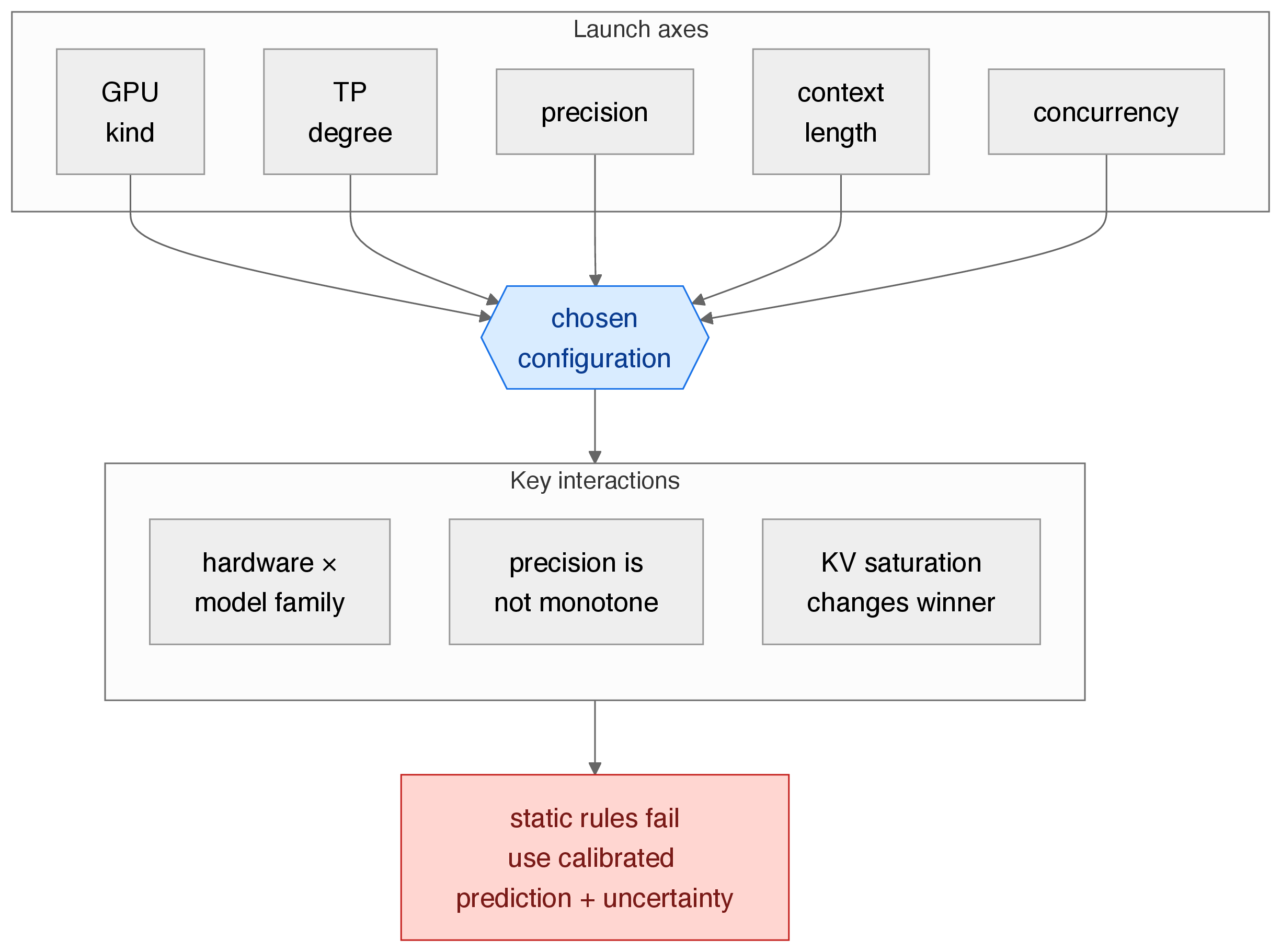
Using these inputs, OmniPilot evaluates and selects from a combinatoric space of configuration arms defined by GPU kind \(\times\) TP degree \(\in\{1,2,4,8\}\) \(\times\) precision \(\in\{\text{bf16, FP8, AWQ, GPTQ}\}\) (Figure 2). The output is a ranked recommendation accompanied by a calibrated cost interval per arm, or an abstention when the request falls outside the system’s measured support envelope. The optimization objective is expected economic utility: the predicted serving value net of node-hour cost, queue wait time, expected-failure restart cost, SLO violation probability, and a KV-saturation penalty.
0.2.3 2.3 The measurement-stale problem↩︎
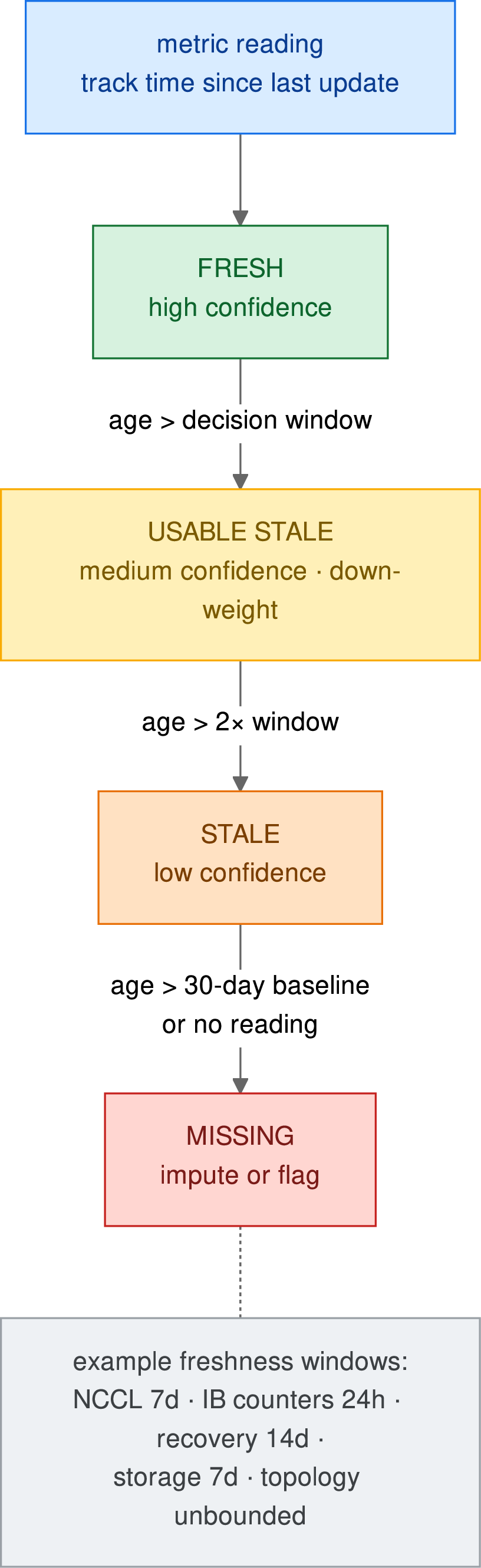
Because the Data Center GPU Manager (DCGM) samples at a 60 s cadence, whole-job averages inadvertently capture low-activity container startup phases. This can severely understate actual serving-time behavior. For instance, restricting averages strictly to the active serving epoch increases measured SM activity from 21% to 51% and power draw from 132 W to 189 W. To prevent this skew, the advisor assigns explicit freshness windows to each metric (Appendix C; Figure 6) and actively down-weights stale measurements.
0.3 3. Method↩︎
0.3.1 3.1 System Architecture↩︎
The OmniPilot architecture (Figure 1) is built around three core, evaluated components: the conformally calibrated cost model, the out-of-distribution abstention layer, and the decision-coupled placement advisor. (Note that two elements within the decision layer—the live resource query and the rule-based fallback triggered upon abstention—serve as operational scaffolding rather than evaluated contributions.)
The system’s predictive intelligence is grounded in two distinct data stores. The personal store (history.jsonl, 1,667 typed rows) maintains the tightly controlled benchmark grid, while the cluster-wide store
(cluster_history.jsonl, 500K jobs) aggregates broad telemetry harvested across all users. To ensure strict data lineage and reproducibility, every logged record enforces a typed kind, a content hash for idempotent deduplication, a
schema version, and a software-stack fingerprint. Appendix C details the underlying collector schemas, gated model updates, recalibration, and benchmark-gate internals.
Two components of the decision layer are operational scaffolding rather than evaluated contributions: the live resource query and the rule-based fallback used after model abstention. The evaluated claims concern the cost model, the abstention layer, and the decision-coupled placement advisor.
Two stores support the system. The personal store (history.jsonl, 1,667 typed rows) holds the controlled benchmark grid. The cluster-wide store (cluster_history.jsonl, 500K jobs) holds the all-users harvest. Every row carries a
typed kind, a content hash for idempotent deduplication, a schema version, and a software-stack fingerprint. Appendix C gives collector schemas, gated model updates, recalibration, and benchmark-gate internals.
0.3.2 3.2 The Inference Cost Model↩︎
0.3.2.1 3.2.1 Design and feature engineering
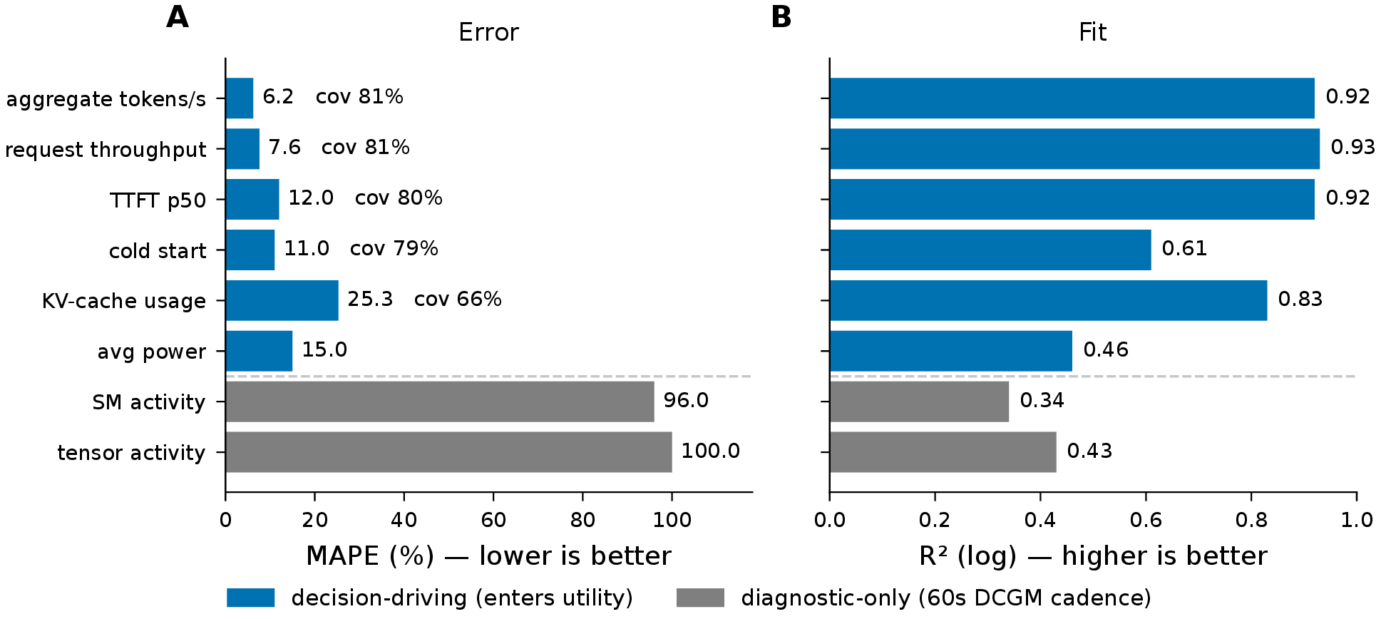
The cost model is a set of gradient-boosted regressors with quantile loss (Figure 4, Appendix A). For each target, it fits the \(\{0.1, 0.5, 0.9\}\) quantiles in log space because target values span orders of magnitude and errors are multiplicative. The model predicts eight targets. Six drive decisions: aggregate tokens/s, request throughput, TTFT (p50), cold-start time, peak KV-cache usage, and average power. Two are diagnostic only: SM- and tensor-core activity. The 60 s DCGM cadence under-resolves these activity targets (\(R^2\)(log) 0.30–0.40), so they never enter the decision utility. A target is fit only when it has at least fifteen labeled rows. Appendix B reports per-target feature exclusions, labeled-row counts, and raw quantile-crossing diagnostics (Table 7).
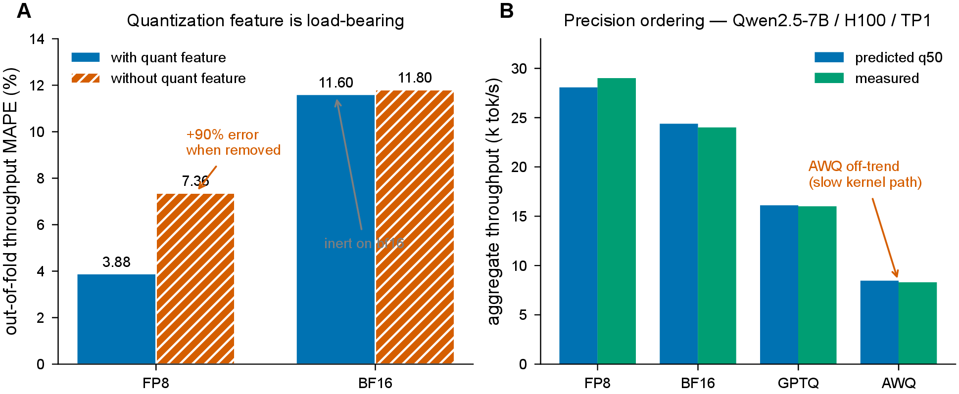
The featurizer encodes roughly 28 features: log-transformed numerics (model size, concurrency, context length, KV pressure, active MoE parameters), linear numerics (TP degree, memory utilization, effective bits), and one-hot encodings over nine model families, five GPU kinds, and four quantization formats. A new axis must be represented before its data is collected. Removing the quantization feature inflated out-of-fold FP8 error from 3.88% to 7.36% (+90%) while leaving bf16 unchanged (Figure 5a; §5.4). The feature is uninformative where precision does not vary and predictive where it does.
0.3.2.2 3.2.2 Calibration, abstention, and accuracy
Prediction intervals use conformalized quantile regression (CQR) [9], [10]. For each target, OmniPilot applies a split-conformal additive offset in log space, calibrated on held-out-cell residuals. This grouped cross-conformal construction achieves 80% coverage on unseen workload cells, compared with 64–69% under a random-fold offset. Beyond the support envelope, conformal intervals fail (§4.3). OmniPilot therefore uses support-distance abstention, rather than interval width alone, as the out-of-distribution guardrail. Appendix C.3 gives construction details.
At fit time, the model stores its training envelope across seven axes. At inference, a support check flags any out-of-envelope axis and downgrades confidence to low, independent of interval width. Section 4.3 shows why this support-distance signal is needed when interval width fails. The measured envelope covers 3–9B models on A100/H100/H200 (51 cells, 96% top-1).
Five-fold cross-validation on 460 rows gives the per-target errors in Table 1. Figure 8 plots the same breakdown.
| Target | MAPE | \(R^2\) (log) | 80% coverage |
|---|---|---|---|
| aggregate tokens/s | 6.2% | 0.92 | 81% |
| request throughput | ~7.6% | 0.93 | ~81% |
| TTFT (p50) | ~12% | 0.92 | 80% |
| cold start | ~11% | 0.61 | ~79% |
| KV-cache usage | 25.3% | ~0.83 | ~66% |
| average power | ~15% | ~0.46 | — |
| SM activity | ~96% | 0.34 | — |
| tensor activity | ~100% | 0.43 | — |
The main decision-driving latency and throughput targets have 6–12% MAPE with log-space \(R^2\) of 0.92–0.93. KV-cache usage and average power are less accurate but still decision-relevant. SM and tensor activity have 96–100% MAPE because the 60 s DCGM cadence under-resolves them; they are diagnostic only.
0.3.3 3.3 Decision Utility and the Launch-Success Prior↩︎
0.3.3.1 3.3.1 Economic utility
OmniPilot ranks arms by utility. The utility equals predicted throughput times runtime times a per-token value, minus compute cost, queue wait, expected failure cost, SLO violation cost, and a KV-saturation penalty. Compute cost is measured in capex-plus-power node-hours.
We calibrate value-per-token by revealed preference. The value \(2\times10^{-7}\) matches an expert operator’s anchors (7B\(\to\)A100, 32B\(\to\)2\(\times\)A100). At this value, joint placement reaches 95% top-1 accuracy with regret 0.003, compared with 0.020 under a throughput-first setting.
A KV-saturation term applies a multiplicative throughput penalty above an occupancy knee of 0.85. This converts KV preemptions into utility cost. Adding the term corrected the Qwen2.5-32B/A100 precision decision without adding data: precision backtest accuracy rose to 96% top-1, and the affected cell’s regret dropped from 0.28.
0.3.3.2 3.3.2 A launch-success prior from cluster data
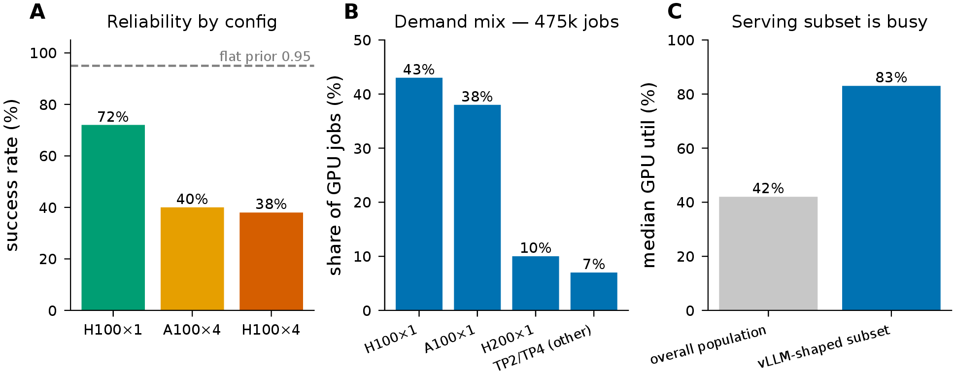
The failure term uses a per-configuration launch-success prior from the cluster-wide harvest (§5.2). A beta-binomial estimator shrinks each configuration toward the pooled rate, so sparsely sampled configurations remain near the pool. Observed cluster success falls to about 38% at TP4, so multi-GPU configurations carry larger expected-failure cost than under the flat 0.95 default. Appendix B reports shrinkage sensitivity.
A regression-gated retraining loop promotes a candidate model only when decision-target MAPE does not regress by more than 0.5 percentage points. One observed cycle, from 447 to 460 rows, satisfied this gate (Appendix C.2).
0.4 4. Evaluation↩︎
0.4.1 4.1 Setup↩︎
The primary results use a frozen 460-row snapshot. It spans six model families, three GPU kinds (A100-40GB, H100-80GB, H200-141GB), four precisions, and TP degrees 1–8 (the full benchmark model list is in Table 8, Appendix B). Holdout cells vary context length (16k, 32k) and concurrency (1500, 2000), and are excluded from training. We reran mechanism checks on the current 476-labeled-row dataset.
Backtests use leakage-free 5-fold GroupKFold grouped by workload cell: base model \(\times\) context \(\times\) concurrency \(\times\) prompt lengths. A model is therefore never evaluated on a cell it trained on. Software is pinned to vLLM 0.11.2. Each row also records a runtime fingerprint, so the update loop can retire stale rows after runtime upgrades (Appendix C.2).
0.4.2 4.2 Placement accuracy↩︎
On 20 multi-precision cells, the advisor reaches 96% top-1 accuracy and 0.001 regret. Always-bf16 has regret 0.144. This gain came from adding the KV-aware utility term (§3.3.1), not from adding data; before the term, the Qwen2.5-32B/A100 cell alone carried 0.28 regret. At the cost-conscious operating point, precision accuracy is 88% with 0.007 regret. In that setting, bf16 is more often sufficient because cost dominates marginal throughput.
We backtested the full joint decision (GPU, TP, and precision) on 65 multi-arm workload cells from the frozen 460-row snapshot (§4.1). At the cost-conscious calibrated value-per-token (§3.3.1), OmniPilot reaches 95% top-1 accuracy and regret 0.003. Bootstrap confidence intervals are [89%, 100%] for top-1 accuracy and [0.000, 0.008] for regret. The no-model baseline has regret 2.71, mainly because it over-provisions Hopper GPUs when an A100 is sufficient. Per-band results (Table 5, Appendix B) show that the 3–9B band has 51 cells and 96% top-1 accuracy. Remaining misses are low-regret H100/H200 tie-breaks.
Table 2 repeats the comparison on the current 476-row dataset (66 cells; §4.1). OmniPilot reaches 92% top-1 accuracy and regret 0.006, consistent with the frozen primary result. It has lower regret than the size rule (1.97), H100/FP8 recipe (1.65), throughput-max policy (4.73), and nearest-neighbor policy (0.72). Cheapest-fit is the closest baseline with 91% top-1 accuracy and regret 0.010. This baseline is competitive because the calibrated operator preference is already cost-conscious, but it cannot choose precision or anticipate KV-saturation cases.
| Policy | Top-1 | Regret |
|---|---|---|
| OmniPilot (advisor) | 92% | 0.006 |
| Cheapest-fit | 91% | 0.010 |
| Size-threshold TP rule | 80% | 1.970 |
| H100/FP8 recipe | 42% | 1.651 |
| Throughput-max (newest GPU) | 3% | 4.728 |
| Nearest-neighbor cell | 70% | 0.722 |
| OmniPilot (bf16-only) | 91% | 0.010 |
| Mean-arm (random) | – | 2.677 |
0.4.3 4.3 Out-of-distribution behavior and calibration↩︎
The holdout sweep used OLMo-2-13B as a new family and 13B size band. It also used Qwen2.5-7B at 16k/32k context and 1500/2000 concurrency. All five cells are outside the measured envelope. For each cell, the canonical model predicted throughput before the run, and the run then measured it (Table 2).
The off-distribution predictions have 24–46% error, compared with roughly 6% in envelope. The conformal intervals cover 0 of 5 points, so interval width alone is not reliable beyond the envelope. The support-distance signal flags all five cells as low-confidence. With only five OOD cells, these numbers illustrate a failure regime rather than estimate an OOD error rate. The supported claim is qualitative: beyond the measured envelope, predictions fail and the abstention layer flags the affected cells.
The confidence label also separates error regimes on in-distribution traffic (Table 6, Appendix B). A leave-one-family-out test (Table ¿tbl:tab:generalization?, Appendix B) shows that related families predict to 11–19% error, while novel architectures degrade to 29–126% and are flagged.
| OOD cell | pred q50 | [q10, q90] | realized | error | covered? | confidence |
|---|---|---|---|---|---|---|
| OLMo-13B (new family) | 17,026 | [14,560, 20,327] | 11,633 | 46% | no | low |
| Qwen-7B ctx 16k | 16,583 | [8,669, 17,815] | 24,167 | 31% | no | low |
| Qwen-7B ctx 32k | 16,538 | [6,545, 17,873] | 24,353 | 32% | no | low |
| Qwen-7B conc 1500 | 23,174 | [8,774, 29,143] | 30,516 | 24% | no | low |
| Qwen-7B conc 2000 | 23,663 | [8,774, 29,953] | 30,944 | 24% | no | low |
Table 4 in Appendix B evaluates the construction in §3.2.2. Held-out-cell recalibration restores in-envelope coverage to 80–81%, compared with 64–69% under random-fold calibration. The interval width cost is 4–12%. A disjoint-cell check in Appendix C.3 gives the same conclusion.
0.4.4 4.4 Ablations and data efficiency↩︎
Table [tab:ablation] in Appendix B summarizes component ablations. Each removal degrades the decision failure mode that the component targets.
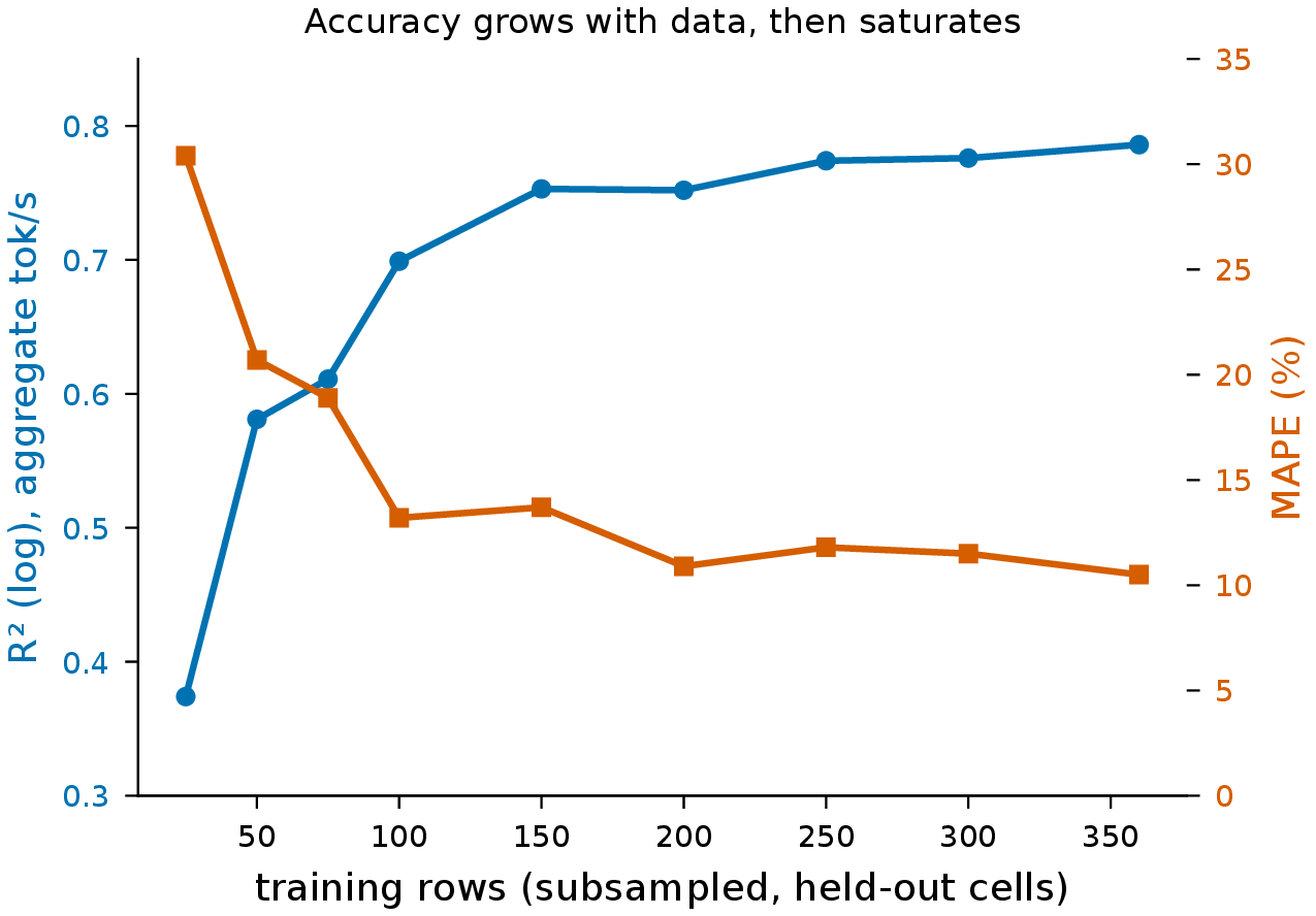
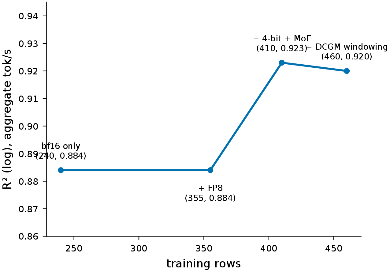
Accuracy tracks axis coverage more than raw row count. Adding 4-bit and MoE data lifts \(R^2\) from the bf16-only baseline to 0.923. In contrast, a fixed-task learning curve shows diminishing returns above \(\sim\)150 rows once the task is already covered (Figures 7, 3).
0.4.5 4.5 Threats to validity↩︎
The results come from a single cluster. Absolute thresholds, including the 0.85 KV knee, freshness windows, and calibrated value-per-token, are deployment-specific. The cluster-wide prior is observational and confounded, so OmniPilot shrinks it toward the pooled rate and uses it only as a launch-success and demand prior, not as placement ground truth. Conformal intervals meet the in-envelope target after recalibration but fail out-of-distribution (§4.3), so support-distance abstention is needed outside the envelope. The update-loop evidence is a single promotion cycle; it demonstrates the mechanism, not a longitudinal trend.
0.5 5. Discussion↩︎
0.5.1 5.1 Cluster telemetry: a negative result↩︎
The scheduler database sees all users, but it records utilization and exit state rather than model, precision, tokens/s, or concurrency. We harvest this all-user job history from Slurm’s accounting database using our HPC_Tools collection scripts [28]
and the jobstats platform [29] (Appendix C.1). Of 500K jobs, only 903 identify as vLLM-like. A cluster-wide throughput advisor is therefore infeasible from infrastructure metadata alone. We report this as an architectural finding and did not
mine job scripts, which would be privacy-sensitive.
0.5.2 5.2 What the cluster data provides↩︎
The harvest provides two usable signals (Figure 9, Appendix B). First, demand is dominated by single-GPU jobs: H100\(\times\)1 accounts for 43% and A100\(\times\)1 for 38%. The benchmark grid covers every high-demand configuration. Second, per-configuration launch success falls from 72% at H100\(\times\)1 to 38% at H100\(\times\)4. OmniPilot shrinks this signal toward the pooled rate and uses it only in the utility’s failure term (§3.3.2), not as a causal hardware-reliability claim. Cross-validating against the cluster population exposed the DCGM windowing artifact in §2.3. We did not blend the two sources because the heavy mixed-job operating point differs from light serving (Appendix B).
0.5.3 5.3 Quantization introduces complex performance dynamics rather than monotonic gains↩︎
Numerical precisions do not follow a simple "fewer bits, faster" rule. While FP8 [8] increases throughput, AWQ [6] is slower on our kernel path, and GPTQ [7] fails entirely for Gemma-2-27b (Figure 5). It is important to note that these performance characteristics reflect out-of-the-box vLLM configurations; while extensive tuning of internal engine parameters might alter these dynamics, we model the baseline operational reality. To capture these nuances, OmniPilot pairs a monotonic effective-bits feature for general compression trends with per-format one-hot features to isolate off-trend behaviors like AWQ (evaluated in §4.2).
KV-cache pressure introduces a second complex interaction driven by cache saturation rather than raw model size. For example, running Qwen2.5-32B on an A100 in bf16 saturates its KV cache (1.00 occupancy), triggering frequent preemptions that spike TTFT to \(\sim\)16 s. Under identical conditions, Mistral-Small-24B maintains sufficient headroom (0.53 occupancy), leaving bf16 as the preferred choice. This non-linear crossover behavior directly motivates the explicit KV-saturation penalty within our decision utility function (§3.3.1).
0.5.4 5.4 Feature-before-data as a general method↩︎
We draw three lessons from the advisor. First, represent a new axis in the featurizer before collecting data on it. The quantization ablation in §3.2.1 shows how this test separates unused features from features that become predictive once the axis varies. Second, some improvements belong in the utility or measurement pipeline rather than the model weights. The KV-saturation term and the DCGM serving-window fix are examples. Third, scheduler metadata can support demand and launch-success priors but cannot recover throughput without workload metadata. A cluster-wide throughput advisor therefore requires instrumentation at the serving layer.
The benchmark gate (Appendix C.4) returns zero value of information at the cost-conscious operating point. This is a structural limitation of the current conditioning rule, which shrinks predictive variance without updating the posterior mean. A useful gate needs posterior mean updates or an equivalent refitting approximation (§5.5).
0.5.5 5.5 Scope and future work↩︎
The primary direction for future research is expanding coverage across broader ML workloads. While OmniPilot can reuse its existing telemetry substrate, extending the system to support training and fault recovery will require developing new targets, utilities, and labels. On the modeling side, the most immediate next step is implementing a benchmark gate that updates posterior means (§5.4). Furthermore, because our current evaluation is constrained to a single-cluster setting, future deployments will require revalidating thresholds across diverse cluster environments. Finally, conducting a longitudinal update-and-drift study over multiple promotion cycles will be essential for assessing the system’s behavioral stability over time.
While the current model successfully leverages cluster telemetry and Slurm job parameters for vLLM inference workloads, it does not currently account for internal engine configurations. Future work will explore how specific vLLM runtime parameters influence inference performance, aiming to integrate these variables into the predictive model to further optimize serving decisions.
Serving systems. vLLM [1], Orca [2], Sarathi-Serve [3], SGLang [4], and AlpaServe [5] optimize execution within a chosen configuration. Recent work optimizes already-chosen deployments through prefill/decode disaggregation [21], [22], KV-cache-centric disaggregation [25], cross-instance migration [23], heterogeneous routing [24], and paging-free KV management [26]. These systems take the model, hardware, and parallelism as given. OmniPilot is upstream: it chooses GPU, TP degree, and precision before submission and abstains outside its measured envelope. Helix [24] is closest in spirit, but it routes over a fixed fleet and does not model quantization or calibrated uncertainty.
Quantization and uncertainty. FP8 [8], GPTQ [7], and AWQ [6] characterize accuracy retention. OmniPilot instead estimates when each precision is beneficial on a given hardware path. The model captures AWQ’s off-trend slowness and hard incompatibilities as measured failure modes. OmniPilot’s intervals use CQR [9], [10], paired with abstention because coverage degrades out-of-distribution. Its benchmark gate applies information-value theory [11] to decide whether a pre-launch probe is worth its node-hours.
Performance modeling and scheduling. Habitat [13], Roofline [14], and MLPerf [15] predict or bound training/inference performance analytically. OmniPilot fits an empirical, decision-coupled model instead. The gating discipline follows production-ML validation [16], [17] and continual-learning regression avoidance [18]. Cluster schedulers such as Gandiva [19] and Tiresias [20] are complementary: they act at submission, while OmniPilot advises before submission.
0.7 7. Conclusion↩︎
OmniPilot optimizes inference workloads within shared, multi-tenant, heterogeneous GPU clusters by transforming hardware configuration selection into a calibrated economic decision. Recognizing that cluster operators have fluctuating priorities—such as weighting power efficiency over token throughput—the system features a flexible utility function that allows optimization goals to be dynamically adjusted along any axis. Acting as a macro-level planner, OmniPilot complements specialized, hardware-level inference engines like vLLM, SGLang, and TensorRT. By combining a conformally calibrated quantile cost model, an out-of-distribution (OOD) abstention layer, a cluster-wide launch-success prior, and a regression-gated update loop, the system reduces placement regret by more than an order of magnitude while its safety shield reliably flags 100 The development of this system also yields three fundamental methodological lessons for cluster-scale machine learning infrastructure. First, new operational axes must be explicitly integrated into the featurizer before data collection begins rather than retroactively. Second, many prediction errors are more effectively resolved through refined utility design or measurement precision rather than simply expanding model capacity. Finally, while standard scheduler metadata (like Slurm logs) successfully provides demand and launch-success priors, it cannot support a cluster-wide throughput advisor because it only records resource allocation—how a GPU was occupied—rather than the specific software workload running on it.
Looking ahead, the primary future direction is expanding OmniPilot’s coverage to broader ML workloads. While the current framework is limited to single-node inference serving, extending the system to handle training and fault-recovery workloads will reuse the existing telemetry substrate while introducing new target metrics and utility functions. Additionally, future research will focus on expanding the planner to support multi-node serving architectures and conducting longitudinal update studies to evaluate how the system manages data drift over extended operational periods.
Acknowledgments↩︎
This work was made possible in part by a gift from the Chan Zuckerberg Initiative Foundation to establish the Kempner Institute for the Study of Natural and Artificial Intelligence at Harvard University. We also thank the Kempner Institute Research Engineering team and the Faculty of Arts and Sciences Research Computing staff for their valuable discussions and support.
0.8 Declarations↩︎
Data and code availability. The benchmark dataset, cost model, and advisor code are in the project repository; the cluster-wide harvest stores users as salted hashes and is not redistributable.
Conflict of interest. The authors declare no competing interests.
Ethics. The cluster-wide harvest uses only scheduler metadata and DCGM metrics, anonymizes users via salted hashing, and does not read job scripts, logs, or payloads.
AI-usage disclosure. Draft prepared with AI assistance for structuring and prose; all quantitative claims derive from the authors’ measured experiments and all citations were verified against primary sources. A venue-specific statement will be generated at submission.
Limitations. See §4.5 and §5.4–5.5.
0.9 References↩︎
[1] W. Kwon, Z. Li, S. Zhuang, Y. Sheng, L. Zheng, C. H. Yu, J. E. Gonzalez, H. Zhang, and I. Stoica, “Efficient Memory Management for Large Language Model Serving with PagedAttention,” in Proc. 29th ACM Symp. Operating Systems Principles (SOSP), 2023. doi:10.1145/3600006.3613165. arXiv:2309.06180.
[2] G.-I. Yu, J. S. Jeong, G.-W. Kim, S. Kim, and B.-G. Chun, “Orca: A Distributed Serving System for Transformer-Based Generative Models,” in Proc. 16th USENIX Symp. Operating Systems Design and Implementation (OSDI), 2022.
[3] A. Agrawal, N. Kedia, A. Panwar, J. Mohan, N. Kwatra, B. S. Gulavani, A. Tumanov, and R. Ramjee, “Taming Throughput-Latency Tradeoff in LLM Inference with Sarathi-Serve,” in Proc. 18th USENIX Symp. Operating Systems Design and Implementation (OSDI), 2024. arXiv:2403.02310.
[4] L. Zheng, L. Yin, Z. Xie, C. Sun, J. Huang, C. H. Yu, S. Cao, C. Kozyrakis, I. Stoica, J. E. Gonzalez, C. Barrett, and Y. Sheng, “SGLang: Efficient Execution of Structured Language Model Programs,” in Advances in Neural Information Processing Systems (NeurIPS), 2024. arXiv:2312.07104.
[5] Z. Li, L. Zheng, Y. Zhong, V. Liu, Y. Sheng, X. Jin, Y. Huang, Z. Chen, H. Zhang, J. E. Gonzalez, and I. Stoica, “AlpaServe: Statistical Multiplexing with Model Parallelism for Deep Learning Serving,” in Proc. 17th USENIX Symp. Operating Systems Design and Implementation (OSDI), 2023. arXiv:2302.11665.
[6] J. Lin, J. Tang, H. Tang, S. Yang, W.-M. Chen, W.-C. Wang, G. Xiao, X. Dang, C. Gan, and S. Han, “AWQ: Activation-aware Weight Quantization for LLM Compression and Acceleration,” in Proc. Machine Learning and Systems (MLSys), 2024. arXiv:2306.00978.
[7] E. Frantar, S. Ashkboos, T. Hoefler, and D. Alistarh, “GPTQ: Accurate Post-Training Quantization for Generative Pre-trained Transformers,” in Proc. Int. Conf. Learning Representations (ICLR), 2023. arXiv:2210.17323.
[8] P. Micikevicius, D. Stosic, N. Burgess, M. Cornea, P. Dubey, R. Grisenthwaite, S. Ha, A. Heinecke, P. Judd, J. Kamalu et al., “FP8 Formats for Deep Learning,” arXiv:2209.05433, 2022.
[9] Y. Romano, E. Patterson, and E. J. Candès, “Conformalized Quantile Regression,” in Advances in Neural Information Processing Systems (NeurIPS), 2019, pp. 3538–3548. arXiv:1905.03222.
[10] A. N. Angelopoulos and S. Bates, “A Gentle Introduction to Conformal Prediction and Distribution-Free Uncertainty Quantification,” arXiv:2107.07511, 2021.
[11] R. A. Howard, “Information Value Theory,” IEEE Trans. Systems Science and Cybernetics, vol. 2, no. 1, pp. 22–26, 1966. doi:10.1109/TSSC.1966.300074.
[12] F. M. Polo, L. Weber, L. Choshen, Y. Sun, G. Xu, and M. Yurochkin, “tinyBenchmarks: Evaluating LLMs with Fewer Examples,” in Proc. Int. Conf. Machine Learning (ICML), 2024. arXiv:2402.14992.
[13] G. X. Yu, Y. Gao, P. Golikov, and G. Pekhimenko, “Habitat: A Runtime-Based Computational Performance Predictor for Deep Neural Network Training,” in Proc. USENIX Annual Technical Conf. (ATC), 2021. arXiv:2102.00527.
[14] S. Williams, A. Waterman, and D. Patterson, “Roofline: An Insightful Visual Performance Model for Multicore Architectures,” Communications of the ACM, vol. 52, no. 4, pp. 65–76, 2009. doi:10.1145/1498765.1498785.
[15] V. J. Reddi, C. Cheng, D. Kanter, P. Mattson, G. Schmuelling, C.-J. Wu et al., “MLPerf Inference Benchmark,” in Proc. ACM/IEEE 47th Int. Symp. Computer Architecture (ISCA), 2020. doi:10.1109/ISCA45697.2020.00045. arXiv:1911.02549.
[16] D. Baylor, E. Breck, H.-T. Cheng, N. Fiedel, C. Y. Foo, Z. Haque, S. Haykal, M. Ispir, V. Jain, L. Koc et al., “TFX: A TensorFlow-Based Production-Scale Machine Learning Platform,” in Proc. 23rd ACM SIGKDD Int. Conf. Knowledge Discovery and Data Mining (KDD), 2017. doi:10.1145/3097983.3098021.
[17] E. Breck, N. Polyzotis, S. Roy, S. E. Whang, and M. Zinkevich, “Data Validation for Machine Learning,” in Proc. Machine Learning and Systems (MLSys), 2019.
[18] M. De Lange, R. Aljundi, M. Masana, S. Parisot, X. Jia, A. Leonardis, G. Slabaugh, and T. Tuytelaars, “A Continual Learning Survey: Defying Forgetting in Classification Tasks,” IEEE Trans. Pattern Analysis and Machine Intelligence, 2021. arXiv:1909.08383.
[19] W. Xiao, R. Bhardwaj, R. Ramjee, M. Sivathanu, N. Kwatra, Z. Han, P. Patel, X. Peng, H. Zhao, Q. Zhang, F. Yang, and L. Zhou, “Gandiva: Introspective Cluster Scheduling for Deep Learning,” in Proc. 13th USENIX Symp. Operating Systems Design and Implementation (OSDI), 2018.
[20] J. Gu, M. Chowdhury, K. G. Shin, Y. Zhu, M. Jeon, J. Qian, H. Liu, and C. Guo, “Tiresias: A GPU Cluster Manager for Distributed Deep Learning,” in Proc. 16th USENIX Symp. Networked Systems Design and Implementation (NSDI), 2019.
[21] Y. Zhong, S. Liu, J. Chen, J. Hu, Y. Zhu, X. Liu, X. Jin, and H. Zhang, “DistServe: Disaggregating Prefill and Decoding for Goodput-optimized Large Language Model Serving,” in Proc. 18th USENIX Symp. Operating Systems Design and Implementation (OSDI), 2024. arXiv:2401.09670.
[22] P. Patel, E. Choukse, C. Zhang, A. Shah, Í. Goiri, S. Maleki, and R. Bianchini, “Splitwise: Efficient Generative LLM Inference Using Phase Splitting,” in Proc. 51st ACM/IEEE Int. Symp. Computer Architecture (ISCA), 2024. arXiv:2311.18677.
[23] B. Sun, Z. Huang, H. Zhao, W. Xiao, X. Zhang, Y. Li, and W. Lin, “Llumnix: Dynamic Scheduling for Large Language Model Serving,” in Proc. 18th USENIX Symp. Operating Systems Design and Implementation (OSDI), 2024. arXiv:2406.03243.
[24] Y. Mei, Y. Zhuang, X. Miao, J. Yang, Z. Jia, and R. Vinayak, “Helix: Serving Large Language Models over Heterogeneous GPUs and Network via Max-Flow,” in Proc. 30th ACM Int. Conf. Architectural Support for Programming Languages and Operating Systems (ASPLOS), 2025. doi:10.1145/3669940.3707215. arXiv:2406.01566.
[25] R. Qin, Z. Li, W. He, M. Zhang, Y. Wu, W. Zheng, and X. Xu, “Mooncake: A KVCache-centric Disaggregated Architecture for LLM Serving,” in Proc. 23rd USENIX Conf. File and Storage Technologies (FAST), 2025. arXiv:2407.00079.
[26] R. Prabhu, A. Nayak, J. Mohan, R. Ramjee, and A. Panwar, “vAttention: Dynamic Memory Management for Serving LLMs without PagedAttention,” in Proc. 30th ACM Int. Conf. Architectural Support for Programming Languages and Operating Systems (ASPLOS), 2025. doi:10.1145/3669940.3707256. arXiv:2405.04437.
[27] Kempner Institute for the Study of Natural and Artificial Intelligence, “The Kempner AI Cluster,” Harvard University. https://kempnerinstitute.harvard.edu/kempner-ai-cluster/.
[28] D. Balamurugan, “HPC_Tools: Utilities for HPC Cluster Telemetry and Job-Data Collection,” GitHub repository. https://github.com/dmbala/HPC_Tools.
[29] Princeton University Research Computing, “Jobstats: A Slurm Job Statistics and Monitoring Platform,” GitHub repository. https://github.com/PrincetonUniversity/jobstats.
0.10 Appendix A: Supplementary Figures↩︎
The following figures supplement the main text; each is referenced from its corresponding section, and all numbers trace to the same measured results as the body.
0.11 Appendix B: Supplementary Tables↩︎
These tables report the evaluation on the current snapshot (476 labeled inference rows parsed from the 561-run grid). The frozen 460-row backtest in §4 is unchanged.
| Target | random-fold cov. | held-out-cell cov. | width \(\times\) |
|---|---|---|---|
| aggregate tokens/s | 64% | 80% | 1.12 |
| TTFT (p50) | 69% | 80% | 1.08 |
| KV-cache usage | 69% | 81% | 1.04 |
Figure 10: |
Figure 11: |
|---|---|
Figure 12: |
Figure 13: |
Figure 14: |
Figure 15: |
Figure 16: |
Figure 17: |
Figure 18: |
Figure 19: |
Figure 20: |

|
 .
.  .
.  .
.  .
.  .
.  .
.  .
.  .
.  .
.  .
.  .
. | Size band | Cells | Top-1 | Regret | Supported |
|---|---|---|---|---|
| \(\le\)2B | 3 | 100% | 0.000 | thin |
| 3–9B | 51 | 96% | 0.003 | yes |
| 10–23B | 2 | 100% | 0.000 | thin |
| \(\ge\)24B | 9 | 89% | 0.008 | thin |
| Confidence | \(n\) | MAPE | 80% coverage | q10–q90 width |
|---|---|---|---|---|
| High | 201 | 18% | 69% | 44% |
| Medium | 52 | 146% | 69% | 143% |
| Low (abstain) | 8 | 39% | 62% | 125% |
| Target | labeled rows | crossing rate |
|---|---|---|
| aggregate tok/s | 476 | 9.7% |
| request throughput | 476 | 8.4% |
| TTFT (p50) | 476 | 1.9% |
| cold start | 472 | 1.1% |
| KV-cache usage | 329 | 10.1% |
| average power | 476 | 0.4% |
| SM activity | 476 | 6.1% |
| tensor activity | 476 | 10.1% |
| Family | Models | Size (B) | Precisions | Runs |
|---|---|---|---|---|
| qwen2 | 6 | 0.5–32 | awq/bf16/fp8/gptq | 236 |
| llama3 | 2 | 8 | awq/bf16/fp8/gptq | 89 |
| deepseek_distill | 1 | 7 | bf16/fp8 | 67 |
| mistral | 4 | 7–46.7 | awq/bf16/gptq | 35 |
| phi | 4 | 3.8–41.9 | bf16 | 23 |
| gemma | 3 | 2–27 | bf16 | 19 |
| other (pythia, olmo) | 2 | 12–13 | bf16 | 7 |
| Total | 22 | 0.5–46.7 | awq/bf16/fp8/gptq | 476 |
@lrr@ Held-out family & \(n\) & MAPE
deepseek_distill & 67 & 11%
llama3 & 89 & 14%
mistral & 35 & 16%
qwen2 & 236 & 19%
other (pythia, olmo) & 7 & 29%
gemma & 19 & 56%
phi & 23 & 126%
Qwen2-7B-Instruct & 4 & 2%
Llama-3.1-8B-Instruct & 11 & 2%
gemma-2-2b-it & 6 & 5%
Phi-3-mini-4k-instruct-3.8B & 6 & 63%
gemma-2-9b-it & 7 & 66%
gemma-2-27b-it & 6 & 67%
0.12 Appendix C: System and Method Details↩︎
0.12.1 C.1 Telemetry collectors and store schema↩︎
Three collectors provide the inference labels. A per-job emitter records cold start, request and aggregate throughput, TTFT, inter-token-latency percentiles, KV usage, and power for each serving run. It also records the serving-window epochs. A per-job
DCGM collector aggregates power and activity. Its serving-window path restricts averages to the recorded [serve_start,serve_end] interval to avoid the staleness artifact in §2.3. A cluster-wide harvester reads all-user jobs from Slurm
sacct with our HPC_Tools collection scripts [28]. It decodes the per-job statistics blob stored in each job’s admin comment by the jobstats platform [29], which is present on roughly 92% of jobs, and stores users as salted hashes
for privacy.
The safety shield consumes GPU-health signals, including XID errors and row-remap failures. The personal store contains 543 job-statistics rows, 481 per-job DCGM rows, and 11 DCGM snapshots alongside the 561 inference runs. Training and recovery collectors also exist in the shared substrate, as do hardware-fingerprinting probes for node admission, FLOP-utilization baselines, and checkpoint throughput. The inference advisor does not consume those signals.
0.12.2 C.2 Gated model updates↩︎
The loop. Every launch produces an inference-run row. Periodic rebuilds backfill realized job statistics and DCGM data, refit a candidate model, and gate that candidate against the incumbent before promotion. This loop carries upstream improvements into production, including the serving-window telemetry fix (§2.3) and new precision or family data.
The no-regression gate. The gate’s decision target is aggregate tokens/s, which drives placement utility. A candidate is promoted only if its decision-target error does not regress by more than 0.5 percentage points and it was trained on at least as many rows as the incumbent. The first fit always promotes. This mirrors validation gates in production ML platforms [16], [17] and regression avoidance in continual learning [18], specialized here to a cost model rather than a classifier.
Provenance and envelope co-evolution. Each version is recorded in a provenance ledger with its training-row count, decision-target metrics, and support envelope. Any recommendation can therefore be traced to a model version. The support envelope is recomputed at each fit, so the abstention boundary changes only when data changes. In the observed run, incorporating holdout data expanded the context bound to 32,768 and the concurrency bound to 2,000. This single promotion cycle moved the dataset from 447 to 460 rows, with MAPE moving from 5.89% to 6.19%.
0.12.3 C.3 Held-out-cell recalibration and the nested confirmation↩︎
The offset is the conformal quantile of the grouped-CV held-out-cell residual pool. It reaches the 80% target on that pool by construction and, under exchangeability, on future cells drawn from the same distribution. The measured quantities are therefore the baseline under-coverage, 64–69%, and the width cost of recalibration, \(\times\)1.04–1.12 (Table 4). The offset is computed once from grouped cross-validation and stored with the model, so deployed intervals use held-out-cell-calibrated widths.
We also test the offset with a nested grouped cross-conformal split. In this check, the offset is sized on workload cells that are disjoint from the cells used to measure coverage. The random-fold offset under-covers again: 66% for aggregate throughput, 73% for TTFT, and 67% for KV-cache usage. The held-out-cell offset restores coverage to 80–84%, with a larger width cost of \(\times\)1.34–1.51. Because the number of cells is small (56–98), these nested estimates have wide bootstrap confidence intervals over cells.
0.12.4 C.4 Benchmark-gate internals↩︎
The value of a benchmark b is the expected improvement in the best achievable utility after observing b. Equivalently, it is the expected best utility after the probe minus the best utility under current uncertainty. We
estimate this quantity with Monte Carlo sampling using \(K=32\) draws from the model’s predictive distribution. The gate then probes sequentially with a 0.2 node-hour budget, depth 3, and epsilon 0.05. It stops on negative
net value, sub-epsilon improvement, budget exhaustion, or exhaustion of the six-benchmark menu. Each benchmark has a closed-form node-hour cost. This is related to efficient-evaluation work [12], but the question differs: whether to spend node-hours
measuring before launch, not how many examples are needed to score a model.
We tested the gate across eight scenarios spanning cost-conscious, throughput-first, and SLO-constrained operating points. The scenarios include close, high-uncertainty arms, such as H100 versus H200 for a 7B model at concurrency 1000. In that case,
predicted throughputs differ by a few percent and intervals span \(\sim\)45% of the median. The v1 condition_on(outcome) shrinks the affected target’s predictive interval by 0.4\(\times\) but leaves the central estimate unchanged. For one arm, a sampled throughput outcome of 37,009 tok/s left the q50 at 29,849 tok/s while narrowing q10–q90 width from \(\sim\)14,200 to
\(\sim\)5,700 tok/s. The conditioned utility therefore equals the unconditioned utility, and the Monte Carlo value of information is zero by construction. A useful fix must refit on augmented data per sample, or otherwise
update the posterior mean. The current point-quantile GBMs do not support that update cheaply.