Geometric Signatures of Reasoning: A Spectral Perspective on Task Hardness
July 02, 2026
Abstract
Chain-of-thought (CoT) reasoning enables large language models (LLMs) to solve complex problems by generating intermediate reasoning steps. While much attention has been paid to the length and content of these reasoning chains, far less is known about their internal geometry. We study the geometry of CoT trajectories in the hidden state space of transformer models, formalizing each reasoning chain as a discrete curve in \(\mathbb{R}^d\) and characterizing it through spectral, positional, and kinematic geometric functionals. We introduce the effective dimension \(d_\rho\) as a measure of trajectory complexity and show theoretically that trajectories with flatter eigenvalue spectra correspond to harder tasks, as they explore more of the hidden dimensions. Lastly, we explore how kinematic features of the trajectory, mean position, positional dispersion, initial and current hidden states, mean velocity, mean speed, and speed dispersion, can be used to predict solution correctness before generation is complete, and may inform future early-stopping strategies. Experimentally, on mathematical reasoning problems from the MATH500 dataset, \(d_\rho\) achieves \(0.93\) AUC in distinguishing easy from hard problems, while kinematic features potentially can predict correctness from only the first \(20\%\) of generated tokens. These correctness signatures transfer across questions of varying difficulty, establishing that the shape of a model’s internal reasoning trajectory is a principled window into both task hardness and solution quality.
1 Introduction↩︎
Large language models (LLMs) have demonstrated remarkable reasoning capabilities through chain-of-thought (CoT) prompting, where models generate intermediate reasoning steps before producing final answers [1]. Recent systems such as OpenAI’s o1 and DeepSeek R1 have shown that scaling test-time compute, allowing models to “think longer”, can dramatically improve performance on complex reasoning tasks [2], [3]. At the same time, it has been observed that simply increasing test-time computation can harm performance, a phenomenon known as overthinking: reasoning length does not directly convert to correct answers [4]. In general, one expects a model to engage in more deliberate reasoning for harder tasks and less for easier ones. Recent theoretical work has further shown that, for transformers trained on an in-context weight prediction task for linear regression, increasing test-time compute can harm performance when the skills required to solve the downstream task are insufficiently represented in the training data [5].
Despite these theoretical and empirical advances, fundamental questions remain: What makes a task hard for a general LLM? How does task difficulty affect the model’s internal representations, and can we predict it from those representations alone? Can we identify promising reasoning paths early, before generation is complete? These questions have profound practical implications: when generating \(n\) candidate solutions to a problem (best-of-\(n\) sampling), can we prioritize which paths to pursue based on the geometry of their early trajectories?
In this paper, we address these questions by studying the geometry of chain-of-thought trajectories in the hidden state space of transformer models. Our key insight is that as an LLM generates tokens during reasoning, the sequence of hidden states traces a discrete curve in \(\mathbb{R}^d\), and the geometric properties of this curve encode information about both task difficulty and solution quality.
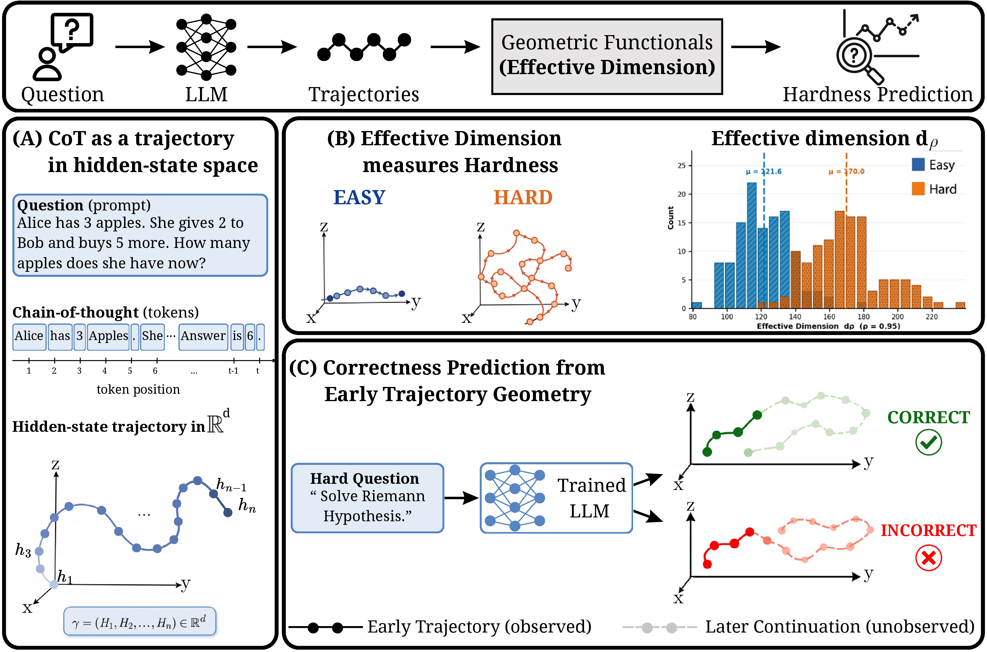
Our contributions are as follows:
Formal Framework for CoT Geometry (Section 3): We formalize CoT reasoning as a discrete curve in \(\mathbb{R}^d\) and introduce geometric functionals that extract spectral, positional, and kinematic properties of reasoning trajectories.
Effective Dimension as Task Complexity (Section 4): We introduce a geometrical function capturing hardness of the task. More precisely, the effective dimension \(d_\rho\) of reasoning curves as a principled measure of task hardness. We further, characterize which curves attain the highest effective dimension, establishing them as geometric representatives of the hardest tasks.
Hardness Prediction (Section 5.3): Using only effective dimension features, we achieve AUC \(> 0.93\) in predicting whether a mathematical problem is easy or hard.
Correctness Prediction (Section 5.2): Seven kinematic and positional features of the trajectory predict solution correctness with AUC \(= 0.806\) from only the first \(20\%\) of generated tokens, with promising implications for early-exit strategies and best-of-\(n\) ranking.
2 Related Work↩︎
Chain-of-thought prompting [1], [6] has emerged as a powerful technique for eliciting multi-step reasoning in LLMs. Recent work has explored scaling test-time compute [7]–[9], with systems like OpenAI o1 [2] and DeepSeek R1 [3] demonstrating strong performance through extended reasoning chains. A complementary line of work has observed that more reasoning is not always better: overthinking can degrade performance when the skills required for a task are underrepresented in training [4]. Our work studies these phenomena from a geometric angle, asking not how long a chain is but what shape it traces in hidden state space.
[5] provide a theoretical analysis of test-time scaling for transformers trained on in-context weight prediction for linear regression. They characterize task hardness via the ratio of the trace with the minimum eigenvalue of the feature covariance matrix, showing that harder tasks require longer chains-of-thought to reach a given error level, and that insufficient task coverage in training can cause additional reasoning steps to hurt performance. Our work is complementary but distinct in two ways. First, we study task hardness empirically in a general LLM rather than deriving it from a tractable linear model. Second, and more fundamentally, we shift the unit of analysis from the output chain to the internal hidden state trajectory: we show that task hardness leaves a geometric signature in the model’s representation space, captured by the effective dimension \(d_\rho\) of the trajectory covariance, and that this quantity alone is highly predictive of problem difficulty
[10] argue that chain-of-thought reasoning offers a unique safety opportunity because, for sufficiently hard tasks, transformers must externalize reasoning through the CoT in order to complete it, making that reasoning in principle observable. They focus on the content of the generated text as the monitoring signal and discuss conditions under which this signal may degrade. Our work operates at a different level: rather than reading the textual content of the chain, we read the geometry of the hidden states that produce it. The two perspectives are complementary, CoT text monitoring and hidden-state trajectory analysis can in principle be combined, but our approach is model-internal and does not rely on the model producing legible natural language reasoning.
[11] study LLM reasoning as a structured trajectory in representation space, extracting hidden states at explicit step boundaries (“Step 1:”, “Step 2:”, …) and showing that these activations form linearly separable, step-specific subspaces that become more pronounced with layer depth. For correctness prediction, they achieve high AUC using late-step trajectory features, and explore inference-time interventions such as activation steering [12] to correct deviating trajectories. Our work shares the trajectory perspective but pursues different goals. Rather than analyzing step-boundary activations, we treat the full token-level hidden state sequence as a continuous curve and characterize it through spectral and kinematic geometric functionals. This allows us to ask whether trajectory geometry encodes task difficulty. We show that the effective dimension \(d_\rho\) of the trajectory covariance, a spectral property of the curve as a whole, predicts whether a problem is easy or hard with high AUC, and we provide a theoretical account of why harder tasks necessarily induce higher-dimensional trajectories. We further show that kinematic features of the trajectory carry an early correctness signal that is detectable from only the first \(20\) percent of generated tokens, opening a practical route to early stopping and best-of-\(n\) ranking without waiting for generation to complete.
Recent work also has proposed geometric frameworks for understanding how LLMs reason. [13] model reasoning as smooth flows in representation space, using the velocity and Menger curvature of the trajectory to show that logical structure, rather than surface semantics, governs the direction and magnitude of these flows. Their focus is on interpretability. Our work takes a complementary direction: we use geometric functionals of the hidden-state trajectory, specifically the spectral effective dimension and kinematic summaries, to predict task difficulty and solution correctness, connecting trajectory geometry directly to downstream performance.
Lastly, [14] show that effective reasoning strategies reduce the intrinsic dimensionality of the learning objective, measured as the minimum number of LoRA parameters needed to fine-tune a model to a given accuracy threshold on GSM8K. They fix the model and vary the reasoning strategy, finding that lower intrinsic dimensionality correlates strongly with better generalization. While both their work and ours use notions of dimensionality to characterize reasoning, the two measures are conceptually distinct. Their intrinsic dimension is a property of the learning problem induced by a reasoning strategy, it requires fine-tuning experiments and measures how compressible a dataset of reasoning chains is. Our effective dimension \(d_\rho\) is a property of a single inference trajectory, it is computed from the covariance of hidden states produced during one forward pass and requires no training. This makes our measure applicable at inference time and enables per-instance predictions of task difficulty and solution correctness.
3 Problem Formulation↩︎
In this section we formalize Chain-of-Thought reasoning and develop a mathematical framework for characterizing its dynamics via Geometrical Functionals. Consider a transformer language model with \(L\) layers and hidden dimension \(d\). Let \(\mathcal{V}\) denote the finite vocabulary, and let \(\mathcal{V}^* := \bigcup_{n=0}^{\infty} \mathcal{V}^n\) denote the set of all finite sequences over \(\mathcal{V}\) (the Kleene star of \(\mathcal{V}\)). Let \(\Delta(\mathcal{V})\) denote the simplex of probability measures over \(\mathcal{V}\). The model defines a map from finite token sequences to probability measures over the next token: \[\mu: \mathcal{V}^* \to \Delta(\mathcal{V}), \quad (x_1, \ldots, x_t) \mapsto \mu(\cdot \mid x_1, \ldots, x_t).\]
As such for each layer \(\ell \in \{1, \ldots, L\}\), the model also produces a hidden state representation in \(\mathbb{R}^{d}\) where \(d\) is the dimension of the latent representation, i.e.,: \[f^{(\ell)}: \mathcal{V}^* \to \mathbb{R}^d, \quad (x_1, \ldots, x_t) \mapsto H_t^{(\ell)}\in \mathbb{R}^{d}.\]
When the layer \(\ell\) is fixed or clear from context, we write \(H_t \equiv H_t^{(\ell)}\). Given the distribution \(\mu(\cdot \mid x_1, \ldots, x_t) \in \Delta(\mathcal{V})\), the next token is selected according to a temperature parameter \(T \geq 0\). In particular, At temperature \(T > 0\), we sample from a tempered distribution: \[X_{t+1} \sim \mu_T(\cdot \mid x_1, \ldots, x_t), \quad \text{where } \mu_T(x) \propto \mu(x)^{1/T}.\]
At temperature \(T = 0\), the distribution concentrates on the mode: \[X_{t+1} = \arg\max_{x \in \mathcal{V}} \mu(x \mid x_1, \ldots, x_t).\] This distinction is fundamental: at \(T = 0\), given a prompt, the generated sequence is unique; at \(T > 0\), the same prompt yields a distribution over sequences.
3.1 The Space of CoT Curves↩︎
At \(T = 0\), token selection is deterministic. Given a prompt, there is exactly one generated sequence of tokens, this motivates the following definition of the space of discrete curves,
Definition 1. Fix a maximum sequence length \(n \in \mathbb{N}\). The space of discrete curves of length \(n\) is \(\mathcal{C}_n := (\mathbb{R}^d)^n\). An element \(\gamma \in \mathcal{C}_n\) is a tuple \(\gamma = (h_1, \ldots, h_n)\) where \(h_{i} \in \mathbb{R}^{d}\).
We have a natural embedding of \(\mathcal{C}_{m} \subseteq \mathcal{C}_n\) for \(m \leq n\) by repeating the last element \(n-m\) times (in practice, we do not apply this padding but instead work directly with variable-length trajectories). Let \(\mathcal{P} \subset \mathcal{V}^*\) denote the space of input prompts. At \(T = 0\), the model defines a deterministic map from the set of prompts to the space of curves. In particular, we have: \[\mathcal{H}: \mathcal{P} \to \mathcal{C}_n, \quad P \mapsto (h_1, \ldots, h_m, h_m, \ldots, h_m),\] where \(m\) is the generation length and the final state \(H_m\) is repeated to fill length \(n\) (stationary extension). As such we introduce the length \(n\) chain of thought as an element in the space of discrete curves of length \(n\). In other words, given a \(\omega \in \mathcal{V}^*\) the length-\(n\) Chain-of-Thought curve is the element \(\mathcal{H}(\omega) = (h_1(\omega), \ldots, h_n(\omega)) \in \mathcal{C}_n\) produced by generation from \(\omega\), with stationary extension if necessary. We characterize CoT curves through real-or vector valued functionals, in particular:
Definition 2. A vector-valued Geometric Functional is a function \(\varphi: \mathcal{C}_n \to \mathbb{R}^{k}\) that extracts geometric properties of curves. The composition \(\varphi \circ \mathcal{H}: \mathcal{V}^* \to \mathbb{R}^{k}\) characterizes how these properties vary across prompts.
As an example, for a curve \(\gamma = (h_1, \ldots, h_n) \in \mathcal{C}_n\), define the centered curve with elements \(\bar{h}_t = h_t - \frac{1}{n}\sum_{i=1}^n h_i\) and its trajectory covariance matrix, defined as \(C(\gamma) := \frac{1}{n} \sum_{t=1}^{n} \bar{h}_t \bar{h}_t^\top = \frac{1}{n} \bar{H}^\top \bar{H} \in \mathbb{R}^{d \times d},\) where \(\bar{H} = [\bar{h}_1, \ldots, \bar{h}_n]^\top \in \mathbb{R}^{n \times d}\). As such \(C\) is a geometrical functional that takes a curve and produces an element in \(\mathbb{R}^{d^2}\).
Let \(\nu_1 \geq \nu_2 \geq \cdots \geq \nu_d \geq 0\) be the eigenvalues of \(C(\gamma)\) ordered in a non-increasing order, then we introduce another such important geometrical functional as follows:
Definition 3. For \(\rho \in (0, 1]\), the Effective Dimension at threshold \(\rho\) is: \[d_\rho(\gamma) := \min\left\{k \in \{1,\ldots,d\} : \frac{\sum_{i=1}^{k} \nu_i}{\mathrm{tr}(C(\gamma))} \geq \rho \right\}.\] This is the minimum number of principal components needed to capture at least \(\rho\) fraction of the total variance.
The effective dimension measures the intrinsic dimensionality of the reasoning trajectory. A low \(d_\rho\) indicates the trajectory lies near a low-dimensional subspace (simple, structured reasoning), while high \(d_\rho\) indicates the trajectory explores many directions (complex, multi-faceted reasoning).
Lastly, we introduce seven additional geometric functionals, which we use in Section 5.2 for correctness prediction. Let \(\gamma = (h_1, \ldots, h_n) \in \mathcal{C}_n\) be a trajectory, and let \(P \in \mathbb{R}^{d \times k}\) denote the top-\(k\) PCA basis fitted on the training set. Define the projected trajectory with elements \(\tilde{h}_t = P^\top h_t \in \mathbb{R}^k\) for \(t = 1, \ldots, n\), and let \(\tilde{\gamma} = (\tilde{h}_1, \ldots, \tilde{h}_n)\) be the projected curve. Note that to prevent data leakage, when a fraction \(\alpha \in (0,1]\) of the trajectory is observed, we restrict to the window \(\tilde{\gamma}^{(\alpha)} = (\tilde{h}_1, \ldots, \tilde{h}_{\lfloor \alpha n \rfloor})\). Noting that our framework is more general and one can extract many other meaningful functional as needed, we define the following functionals \(\varphi: \mathcal{C}_n \to \mathbb{R}^{5k+2}\) below.
Examples (Kinematic and Positional Geometric Functionals). Given a projected trajectory \(\tilde{\gamma} = (\tilde{h}_1, \ldots, \tilde{h}_m)\) for some \(m \leq n\), define the velocity increments \(\Delta_t := \tilde{h}_{t+1} - \tilde{h}_t \in \mathbb{R}^k\) for \(1 \leq \forall t \leq m-1\). The seven geometric functionals are:
Mean position, defined as \(\mu(\tilde{\gamma}) \;=\; \frac{1}{m}\sum_{t=1}^{m} \tilde{h}_t \;\in\; \mathbb{R}^k.\)
Positional dispersion, the coordinate-wise standard deviation: \[\sigma(\tilde{\gamma}) \;=\; \left(\frac{1}{m}\sum_{t=1}^{m} \bigl(\tilde{h}_t - \mu(\tilde{\gamma})\bigr)^{\odot 2} \right)^{\odot 1/2} \;\in\; \mathbb{R}^k,\] where \(\odot\) denotes elementwise operations.
Initial hidden state, the first token representation of the projected trajectory, i.e., \(\tilde{h}_1 \;\in\; \mathbb{R}^k.\)
Final hidden state, the last token representation of the projected trajectory, i.e., \(\tilde{h}_m \;\in\; \mathbb{R}^k.\)
Mean velocity, the average of successive differences: \[\bar{v}(\tilde{\gamma}) \;=\; \frac{1}{m-1}\sum_{t=1}^{m-1} \Delta_t \;\in\; \mathbb{R}^k.\]
Mean speed, the average step-wise Euclidean norm: \[\bar{s}(\tilde{\gamma}) \;=\; \frac{1}{m-1}\sum_{t=1}^{m-1} \|\Delta_t\|_2 \;\in\; \mathbb{R}.\]
Speed dispersion, the standard deviation of step-wise speeds: \[\sigma_s(\tilde{\gamma}) \;=\; \left(\frac{1}{m-1}\sum_{t=1}^{m-1} \bigl(\|\Delta_t\|_2 - \bar{s}(\tilde{\gamma})\bigr)^2 \right)^{1/2} \;\in\; \mathbb{R}.\]
The full feature vector is the concatenation \[\varphi(\tilde{\gamma}) \;=\; \Bigl(\mu,\;\sigma,\;\tilde{h}_1,\;\tilde{h}_m,\; \bar{v},\;\bar{s},\;\sigma_s\Bigr) \;\in\; \mathbb{R}^{5k+2}.\]
Note that mean velocity telescopes to \(\frac{1}{m-1}(\tilde{h}_m - \tilde{h}_1)\), making it a linear function of the already-included initial and final states. We retain it for completeness and its natural connection to mean speed and speed dispersion.
At temperature \(T > 0\), the same prompt could yields different curves at each generation time. Our formulation can extend to this framework: \[\mathcal{H}: \mathcal{V}^* \to \Delta(\mathcal{C}_n),\] where \(\Delta(\mathcal{C}_n)\) denotes distributions over curves. The induced distribution arises from the autoregressive measure: \[\mathbb{P}_{\mu_T}(v_1, \ldots, v_n) = \prod_{t=1}^{n} \mu_T(v_t \mid x_1, \ldots, x_k, v_1, \ldots, v_{t-1}).\]
4 Effective Dimension as Task Complexity↩︎
This section develops the theoretical core of the paper. We prove general spectral bounds for any covariance matrix, showing via a majorization argument that flat spectra maximize effective dimension (§4.1) and provide finite-sample stability. All proofs are in Appendix 7.
4.1 Spectral Bounds and the Role of Flatness↩︎
The effective dimension of any PSD matrix is controlled by its eigenvalue spread. These are purely linear-algebraic facts, independent of any dynamical model.
Proposition 1 (Spectral Bounds). For any PSD matrix \(C\) with eigenvalues \(\nu_1 \geq \cdots \geq \nu_d \geq 0\), \(\nu_1 > 0\): \[\lceil \rho \, \mathrm{tr}(C)/\nu_1 \rceil \;\leq\; d_\rho(C) \;\leq\; \lceil \rho \, \mathrm{tr}(C)/\nu_d \rceil,\] the upper bound requiring \(\nu_d > 0\).
Proof sketch. Let \(r := d_\rho(C)\). The lower bound follows from \(\rho \mathrm{tr}(C) \leq \sum_{j \leq r} \nu_j \leq r \nu_1\), giving \(r \geq \lceil \rho \mathrm{tr}(C)/\nu_1 \rceil\). The upper bound follows from \(\sum_{j \leq r-1} \nu_j < \rho \mathrm{tr}(C)\) and \(\nu_j \geq \nu_d\), giving \((r-1)\nu_d < \rho \mathrm{tr}(C)\), hence \(r \leq \lceil \rho \mathrm{tr}(C)/\nu_d \rceil\).The complete argument is in Appendix 7. ◻
The ratio \(T/\nu_d\) is similar (they used covariance of the data rather than the dynamic) to the hardness measure of [5]; the upper bound shows it controls \(d_\rho\), but loosely. When the spectrum is flat, the bounds coincide at \(\lceil \rho d\rceil\). Flatness is extremal in a stronger sense, captured by majorization.
Definition 4. For \(x, y \in \mathbb{R}^d\), we say \(x\) is majorized by \(y\), written \(x \prec y\), if \[\sum_{i=1}^k x_{[i]} \;\leq\; \sum_{i=1}^k y_{[i]} \quad \text{for all } k = 1, \ldots, d-1, \quad \text{and} \quad \sum_{i=1}^d x_{[i]} = \sum_{i=1}^d y_{[i]},\] where \(x_{[1]} \geq \cdots \geq x_{[d]}\) is the decreasing rearrangement of \(x\). Informally: \(x\)’s mass is more “spread out” than \(y\)’s, but both have the same total [15].
Majorization gives us a precise way to compare how “peaked” two spectra are. We use it to show that the flat spectrum \(\nu^\star\) is the most spread-out among all spectra with the same trace, and achieves the highest effective dimension. More formally we have:
Proposition 2 (Flat Spectrum Maximizes Effective Dimension). Let \(C\) be PSD with eigenvalues \(\nu \in \mathbb{R}^d\) and trace \(\mathrm{tr}(C)\). Let \(\nu^\star := (\mathrm{tr}(C)/d, \ldots, \mathrm{tr}(C)/d)\), the flat spectrum with the same total. Then:
\(\nu^\star \prec \nu\): the flat spectrum is majorized by any other spectrum with the same total.
\(d_\rho(C) \leq d_\rho(C^\star) = \lceil \rho d\rceil\).
Proof sketch. We first show \(\nu^\star \prec \nu\): since both vectors have total \(\mathrm{tr}(C)\), this reduces to \(\sum_{i \leq k} \nu_i \geq k\mathrm{tr}(C)/d\), i.e., the top-\(k\) average is at least the overall mean. If not, then \(\nu_k\) (and hence every \(\nu_j\) with \(j > k\), by decreasing order) is also below \(\mathrm{tr}(C)/d\), so \(\mathrm{tr}(C) = \sum_i \nu_i < \mathrm{tr}(C)\), a contradiction. The second one follows by definition and using part 1. The complete argument is in Appendix 7. ◻
4.2 Stability under small Perturbation↩︎
The following framework-independent and purely linear-algebraic result shows that if two covariance matrices are \(\epsilon\)-close in operator norm(which is \(\epsilon\)-close in operator norm (\(\|\widehat{C} - C\|_{\mathrm{op}} := \max_{\|v\|=1}\|(\widehat{C}-C)v\|\)), their effective dimensions are also close.
Theorem 3. Let \(C, \widehat C\) be PSD with \(\|\widehat C - C\|_{\mathrm{op}} \leq \epsilon\) and \(\mathrm{tr}(C) > 0\). Assume \(d\epsilon \leq \mathrm{tr}(C)/2\). Define \(F(j) := \sum_{i\leq j}\nu_i/\mathrm{tr}(C)\) where \(\nu_i\) are the decreasingly-sorted eigenvalues of \(C\). Then \[\label{eq:stability} \bigl|d_\rho(\widehat C) - d_\rho(C)\bigr| \;\leq\; \#\!\left\{ j \in \{1,\ldots,d\} : |F(j) - \rho| \leq \tfrac{4d\epsilon}{\mathrm{tr}(C)}\right\}.\qquad{(1)}\] In particular, if the cumulative mass function \(F\) crosses level \(\rho\) transversally (i.e., \(F\) has no index within distance \(4d\epsilon/\mathrm{tr}(C)\) of \(\rho\)), then \(d_\rho(\widehat C) = d_\rho(C)\).
Proof sketch. The argument proceeds in three steps. First, recall Weyl’s inequality: for symmetric matrices \(A, B \in \mathbb{R}^{d \times d}\) with eigenvalues sorted in decreasing order, \(|\lambda_k(A + B) - \lambda_k(A)| \leq \|B\|_{\mathrm{op}}\) for every \(k\). Applied with \(A = C\) and \(B = \widehat{C} - C\), this gives \(|\hat{\nu}_k - \nu_k| \leq \epsilon\) for all \(k\): each eigenvalue of \(\widehat{C}\) is within \(\epsilon\) of the corresponding eigenvalue of \(C\). Summing across \(k\), we also get \(|\mathrm{tr}(\widehat{C}) - \mathrm{tr}(C)| \leq d\epsilon\), and similarly the partial sums \(S_j := \sum_{i \leq j} \nu_i\) and \(\widehat{S}_j\) differ by at most \(d\epsilon\).
Second, we propagate this to the cumulative-mass function \(F(j) := S_j / \mathrm{tr}(C)\). Using the algebraic identity \(\widehat{S}_j \mathrm{tr}(C) - S_j \mathrm{tr}(\widehat{C}) = (\widehat{S}_j - S_j)\mathrm{tr}(C) + S_j (\mathrm{tr}(C) - \mathrm{tr}(\widehat{C}))\) and bounding each piece via the triangle inequality, we obtain \(|\widehat{F}(j) - F(j)| \leq 4d\epsilon / \mathrm{tr}(C) =: \delta\).
Finally, since \(d_\rho\) is the first index at which \(F\) reaches \(\rho\), and \(|F(j) - \widehat{F}(j)| \leq \delta\) everywhere, the two effective dimensions can only disagree at indices where \(F(j)\) lies within \(\delta\) of \(\rho\): away from this band, \(F\) and \(\widehat{F}\) agree on whether the threshold has been crossed. Counting such indices yields ?? . In particular, if \(F\) jumps past \(\rho\) transversally at a single index, with no \(j\) satisfying \(|F(j) - \rho| \leq \delta\), then \(d_\rho(\widehat{C}) = d_\rho(C)\) exactly. The complete argument is in Appendix 7. ◻
5 Experiments↩︎
5.1 Experimental Setup↩︎
5.1.0.1 Model.
We use Qwen2.5-0.5B-Instruct [16], a decoder-only transformer with 24 layers and hidden dimension 896. Despite its small size, it produces well-structured reasoning chains and allows us to extract hidden states at every layer and token position without prohibitive memory cost.
5.1.0.2 Dataset.
We focus on three categories from the MATH500 dataset [17]: Algebra and Counting & Probability and Precalculus. Problems
in the MATH500 dataset are labeled with difficulty annotations ranging from \(1\)-\(5\). We consider the problems with annotations of \(1\), \(3\) and \(5\), which we respectively label as easy, medium and hard.
We use a fixed set of \(9\) (probability had \(2\) easy question rather than \(3\)) questions per category, drawn to ensure a balanced difficulty split. In the case of comparing effective dimension for task difficulty, we only use questions labeled as easy or hard (i.e. annotated as \(1\) or \(5\)).
5.1.0.3 Trajectory Collection.
For each problem, we generate 10 reasoning trajectories at temperature \(T = 0.7\) using two chain-of-thought prompting styles (medium and long which, which are provided in the appendix), pooled for analysis. Each trajectory is generated autoregressively with a maximum of 800 tokens. We extract the hidden state \(h_t^{(\ell)} \in \mathbb{R}^{896}\) at every generated token position \(t\) for all layers \(\ell \in \{0, \ldots, 23\}\), yielding a trajectory matrix \(H^{(\ell)}\) per layer per run. Correctness is determined by a symbolic answer checker combining SymPy expression matching and string normalization against the ground-truth boxed answer.
5.1.0.4 Features for Correctness Prediction.
For each trajectory, we project \(H^{(\ell)}\) onto the top 15 PCA components fitted on the training set, then extract seven kinematic and positional features from the windowed portion of the projected trajectory (which are defined in section 3.1): mean position, positional dispersion (standard deviation), initial hidden state, final hidden state of the truncated trajectories, mean velocity (mean of successive differences), mean speed (mean of step-wise norms), and speed dispersion. Features are standardized before classification.
5.1.0.5 Evaluation Protocol.
For correctness prediction, we use a stratified question-level 80/20 train/test split, repeated over 5 random seeds, ensuring that all trajectories from a given question appear entirely in train or entirely in test. We report AUC-ROC (Area Under the Receiver Operating Characteristic curve) and AUPRC (Area Under the Precision–Recall Curve) with \(\pm\) std across splits. For classifiers we use logistic regression (LR; \(\ell_2\) regularization \(C = 0.1\)), a two-layer MLP (hidden sizes 64 and 32, early stopping, \(\ell_2\) regularization \(\alpha = 0.01\)), and a two-layer GRU (hidden dim 64). We highlight AUPRC because our central question is whether trajectory geometry can rank correct solutions above incorrect ones. AUPRC summarizes this ranking through precision (how many of the trajectories flagged as correct actually are) and recall (how many of the truly correct trajectories are recovered) across all thresholds. This directly reflects our intended use, deciding which of the many candidate trajectories for a given question to continue, since a high-precision, high-recall score lets us concentrate on promising trajectories and potentially reach a correct solution faster.
5.2 Experiment 1: Correctness Prediction from Trajectory Geometry↩︎
We ask whether the geometry of a reasoning trajectory predicts whether it will reach a correct answer, and how early in generation this signal emerges.
5.2.0.1 Cross-question generalization.
Figure 2 shows AUPRC and AUC-ROC results for correctness prediction as a function of the fraction of the trajectory observed, for the LR, MLP, and GRU classifiers, under a stratified question-level 80/20 split averaged over 5 seeds. LR achieves AUC \(= 0.806 \pm 0.132\) at \(20\%\) observation and \(0.839 \pm 0.111\) at \(100\%\), with AUPRC remaining stable around \(0.868\) throughout. MLP reaches AUC \(= 0.723 \pm 0.154\) at \(20\%\), dips at \(30\%\), then recovers to \(0.828 \pm 0.093\) at \(100\%\). The GRU behaves qualitatively differently: it achieves AUC \(= 0.641 \pm 0.215\) at \(20\%\), peaks at \(0.754 \pm 0.078\) at \(70\%\), and then drops to \(0.577 \pm 0.144\) at \(100\%\), barely above chance.

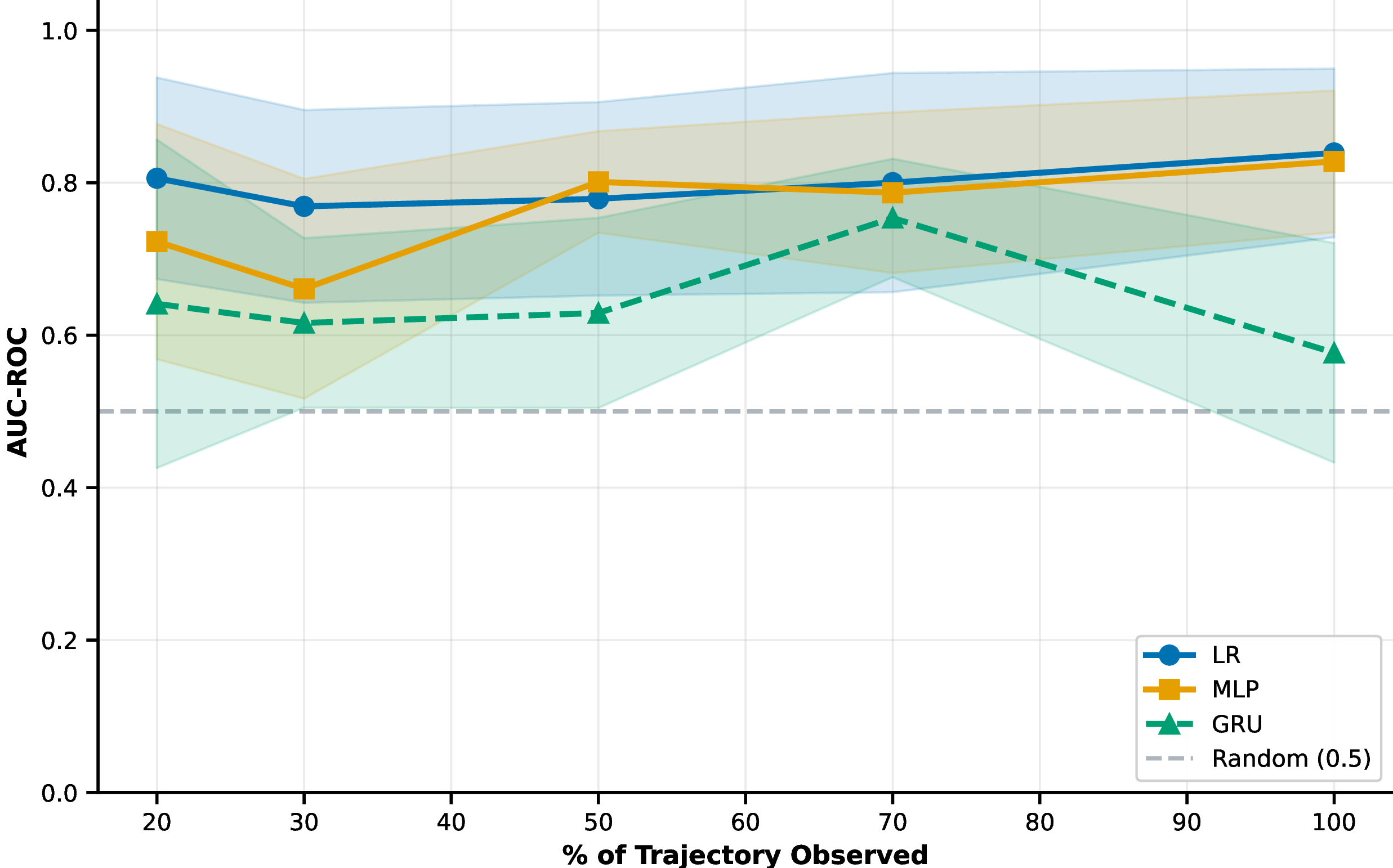
Figure 2: Correctness is detectable from early trajectory geometry. (Left) AUPRC as a function of the fraction of the trajectory observed. (Right) AUC-ROC as a function of the fraction of the trajectory observed. Kinematic and positional features extracted from a windowed prefix of the reasoning trajectory predict whether the trajectory will reach a correct answer before generation is complete. The train/test split is at the question level, using an 80/20 split across five seeds..
5.2.0.2 Within-question prediction.
To understand the ceiling of the correctness signal, we also evaluate a setting where trajectories from the same question can appear in both train and test, while ensuring no trajectory is included in both (i.e. there is no data leakage, but rather leakage at the question level) with 5-fold cross-validation over the set of all pooled trajectories. Here LR achieves AUC \(\approx 0.90\) and MLP achieves AUC \(\approx 0.91\) using only \(20\%\) of the trajectory, with negligible improvement as more tokens are observed (Table 1). This confirms that the geometric signal for correctness is saturated very early, and that the gap between within-question (\(0.90\)) and cross-question (\(0.81\)) performance represents the portion of the signal that is question-specific rather than universally transferable, or that our sample size was not high enough to generalize to such an extent.
| Trajectory % | Logistic Regression | MLP | ||
| AUC | Std | AUC | Std | |
| 20% | 0.902 | 0.012 | 0.912 | 0.023 |
| 50% | 0.902 | 0.016 | 0.914 | 0.015 |
| 100% | 0.919 | 0.017 | 0.909 | 0.022 |
5.3 Experiment 2: Difficulty Prediction via Effective Dimension↩︎
We ask whether the effective dimension \(d_\rho\) of the hidden-state trajectory can predict whether a problem is easy or hard (MATH500 difficulty of \(1\) vs. \(5\)), without any access to the answer or the model’s output. For each problem, at layer \(\ell = 12\), we compute \(d_\rho(H^{(\ell)}, \rho)\) at \(\rho \in \{0.90, 0.95, 0.99\}\), yielding a three-dimensional feature vector per trajectory. We then run leave-one-question-out cross-validation: for each test question, we train an LR or MLP classifier on the effective dimension features from all other questions, and predict whether the test question is easy or hard.
5.3.0.1 Results.
Figure 3 (left) shows AUC-ROC as a function of layer for both classifiers. Effective dimension is predictive at every layer, with AUC rising from \(0.81\) at layer 0 to \(0.93\) at layer 21. Prediction is consistent and robust: even the earliest layers achieve AUC well above chance, and the signal strengthens through the network. The best layer is layer 21 (MLP AUC \(= 0.93\), accuracy \(= 86.8\%\)). Figure 3 (right) shows the distribution of \(d_\rho\) at layer 21 (\(\rho = 0.95\)) for easy and hard problems. The separation is apparent: hard problems have mean effective dimension \(\mu \approx 170\) versus \(\mu = 121.6\) for easy problems, a \(40\%\) gap, with a t-test \(p\)-value of \(5.79 \times 10^{-166}\). Hard trajectories explore a substantially higher-dimensional subspace of the model’s representation space, providing strong evidence for the relationship between effective dimension and task hardness.
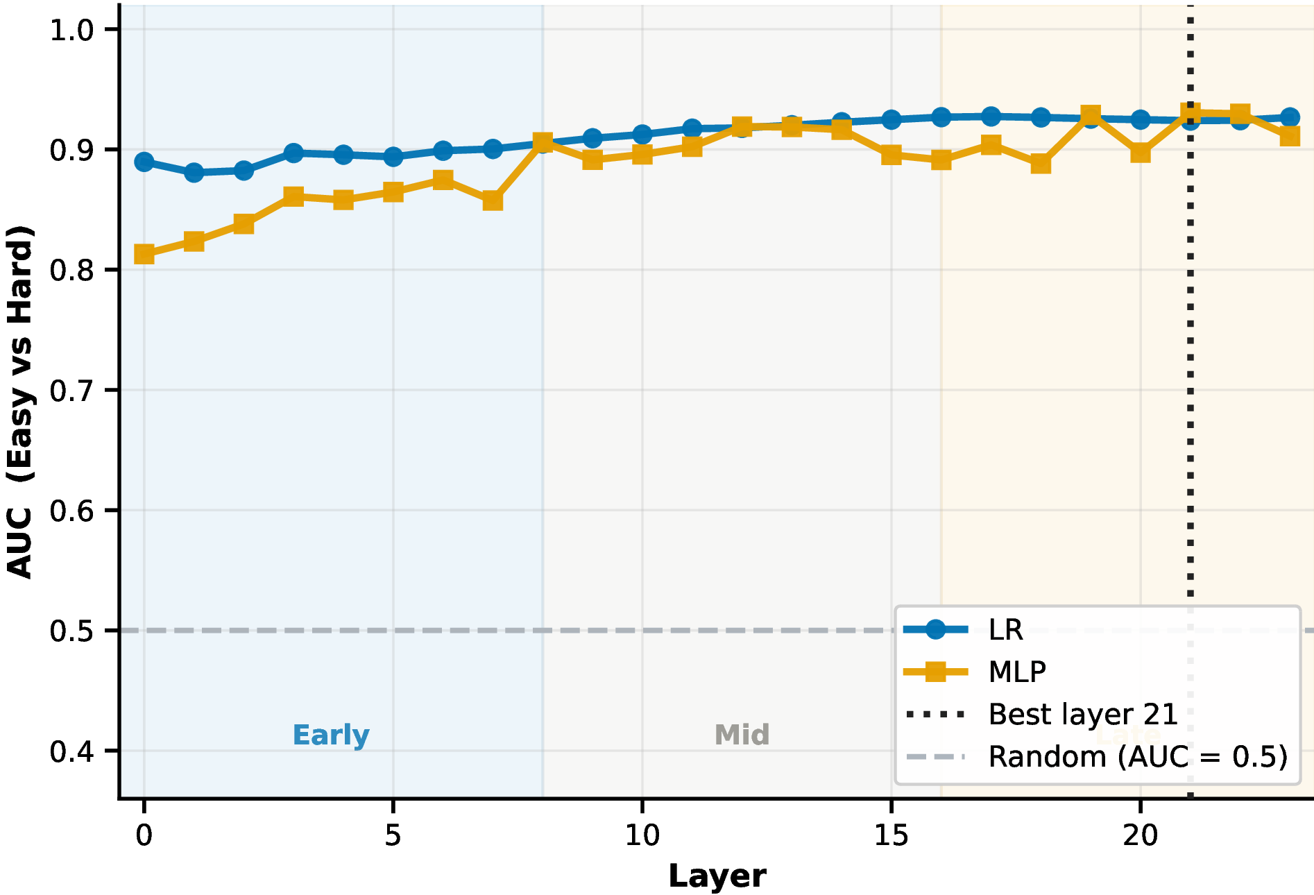
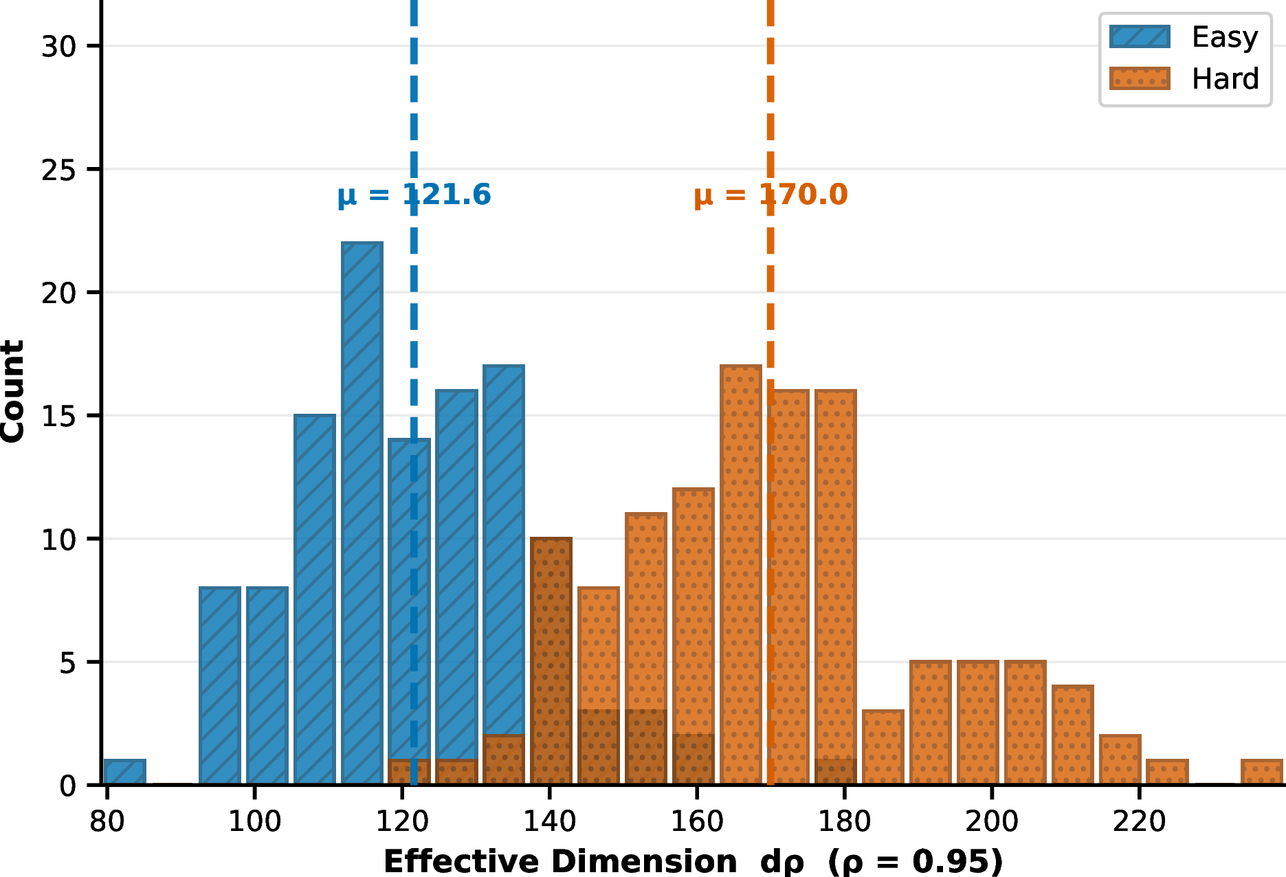
Figure 3: Effective dimension predicts task difficulty. (Left) AUC for easy vs.hard difficulty prediction across all 24 layers. Effective dimension achieve AUC \(> 0.9\) from layer 8 onward, peaking at \(0.93\) at layer 21. (Right) Distribution of \(d_\rho\) (\(\rho = 0.95\)) at layer 21. Hard problems exhibit \(40\%\) higher effective dimension than easy ones (\(p = 5.79 \times 10^{-166}\)). The spectral geometry of the hidden-state trajectory encodes task hardness across all layers, with the signal strengthening toward the final layers..
6 Conclusion↩︎
We study the geometry of chain-of-thought reasoning trajectories in transformer hidden state space. Formalizing each reasoning chain as a discrete curve in \(\mathbb{R}^d\), we introduced the effective dimension \(d_\rho\) as a spectral measure of trajectory complexity and show theoretically that harder tasks necessarily induce higher-dimensional trajectories. Empirically, \(d_\rho\) predicts problem difficulty with AUC \(> 0.93\) via leave-one-question-out cross-validation, with hard problems exhibiting \(40\%\) higher effective dimension on average than easy ones. For correctness prediction, seven kinematic features of the trajectory achieve AUC \(= 0.806\) from only the first \(20\%\) of generated tokens under a question-level split, with a simple logistic regression outperforming a GRU on the full sequence, suggesting there are interesting signal lies in coarse geometric structure. Together, these results establish trajectory geometry as a practical window into both task hardness and solution quality.
Limitations. Our experiments use a single small model and three MATH500 categories, so generalization to larger models and other domains remains open. Our theoretical analysis connects spectral flatness to effective dimension but does not fully explain how task difficulty induces this flatness in a trained transformer. Finally, our correctness prediction is evaluated in terms of AUC; translating this into concrete early-stopping or best-of-\(n\) gains is left for future work.
Acknowledgments↩︎
AJ was supported in part by the NSF Award DMS-2311024, an Amazon Faculty Research Award, an Adobe Faculty Research Award, and an iORB grant form USC Marshall School of Business.
7 Proofs↩︎
In the following proofs, for simplicity of the notations we used \(T := \mathrm{tr}(C)\).
7.1 Proof of Proposition 1↩︎
Proof. Let \(r := d_\rho(C)\). By definition of \(d_\rho\), \(r\) is the smallest integer with \(\sum_{j=1}^{r}\nu_j \geq \rho T\), so we have \[\sum_{j=1}^{r}\nu_j \;\geq\; \rho T \quad\text{and}\quad \sum_{j=1}^{r-1}\nu_j \;<\; \rho T. \label{eq:effdim-def}\tag{1}\]
Lower bound. Since the eigenvalues are sorted in decreasing order, \(\nu_j \leq \nu_1\) for all \(j\). Summing over \(j=1,\ldots,r\): \[\rho T \;\leq\; \sum_{j=1}^{r}\nu_j \;\leq\; r \cdot \nu_1.\] Dividing by \(\nu_1 > 0\) gives \(r \geq \rho T/\nu_1\). Since \(r\) is a positive integer, \(r \geq \lceil \rho T/\nu_1\rceil\).
Upper bound. Since \(\nu_j \geq \nu_d\) for all \(j \leq r-1\), summing: \[(r-1) \cdot \nu_d \;\leq\; \sum_{j=1}^{r-1}\nu_j \;<\; \rho T,\] where the strict inequality is from 1 . Hence \(r-1 < \rho T/\nu_d\), and integrality gives \(r \leq \lceil \rho T / \nu_d\rceil\). ◻
7.2 Proof of Proposition 2↩︎
Proof. (1) \(\nu^\star \prec \nu\). Both vectors have the same total \(T\), so the equality condition in Def. 4 holds. We must show \(\sum_{i=1}^k \nu^\star_i \leq \sum_{i=1}^k \nu_i\) for every \(k\), i.e., \(kT/d \leq \sum_{i=1}^k \nu_i\). Equivalently, we must show the top-\(k\) average of \(\nu\) is at least the overall average: \[\frac{1}{k}\sum_{i=1}^k \nu_i \;\geq\; \frac{T}{d}.\]
Suppose for contradiction that \(\frac{1}{k}\sum_{i=1}^k \nu_i < T/d\). Since \(\nu\) is sorted decreasingly, \(\nu_k \leq \frac{1}{k}\sum_{i=1}^k \nu_i < T/d\) and \(\nu_j \leq \nu_k < T/d\) for all \(j \geq k\). Then \[T \;=\; \underbrace{\sum_{i=1}^k \nu_i}_{< kT/d} \;+\; \underbrace{\sum_{i=k+1}^d \nu_i}_{< (d-k)T/d} \;<\; \frac{kT}{d} + \frac{(d-k)T}{d} \;=\; T,\] a contradiction. Hence the top-\(k\) average is at least \(T/d\), and \(\nu^\star \prec \nu\).
(2) \(d_\rho\) is maximized at the flat spectrum. Let \(r^\star := d_\rho(C^\star) = \lceil \rho d\rceil\) (directly, since \(\sum_{i=1}^{r^\star} \nu^\star_i = r^\star T/d \geq \rho T\) iff \(r^\star \geq \rho d\)). Applying part (1) at \(k = r^\star\): \[\sum_{i=1}^{r^\star} \nu_i \;\geq\; \sum_{i=1}^{r^\star} \nu^\star_i \;\geq\; \rho T.\] By definition of \(d_\rho\) as the smallest such \(r\), \(d_\rho(C) \leq r^\star = d_\rho(C^\star)\).
Equality condition. Equality throughout requires \(\nu^\star \prec \nu\) to be an equality of partial sums at every \(k\), forcing \(\nu_i = T/d\) for all \(i\), i.e., \(\nu = \nu^\star\). ◻
7.3 Proof of Theorem 3↩︎
Proof. Before we prove this, we recall Weyl inequality which states, for any symmetric matrices \(A, B \in \mathbb{R}^{d \times d}\) with eigenvalues sorted in decreasing order, \[\bigl|\lambda_k(A + B) - \lambda_k(A)\bigr| \;\leq\; \|B\|_{\mathrm{op}} \qquad \text{for all } k = 1, \ldots, d.\] where \(\|B\|_{\mathrm{op}} := \text{max}(|\lambda_{1}(B)|,|\lambda_d(B)|)\). In particular, taking \(A = C\) and \(B = \widehat{C} - C\) gives \(|\hat{\nu}_k - \nu_k| \leq \|\widehat{C} - C\|_{\mathrm{op}}\) which we use shortly. Let \(\nu_1 \geq \cdots \geq \nu_d\) and \(\hat{\nu}_1 \geq \cdots \geq \hat{\nu}_d\) be the decreasingly-sorted eigenvalues of \(C\) and \(\widehat C\). Weyl’s inequality for Hermitian matrices gives \(|\hat{\nu}_j - \nu_j| \leq \|\widehat C - C\|_{\mathrm{op}} \leq \epsilon\) for every \(j\). Summing: \(|\mathrm{tr}(\widehat C) - \mathrm{tr}(C)| = |\sum_j (\hat{\nu}_j - \nu_j)| \leq d\epsilon\). Now, let \(S_j := \sum_{i=1}^j \nu_i\) and \(\widehat S_j := \sum_{i=1}^j \hat{\nu}_i\). By Weyl again, \(|\widehat S_j - S_j| \leq j\epsilon \leq d\epsilon\).
Define \(F(j) := S_j/\mathrm{tr}(C)\) and \(\widehat F(j) := \widehat S_j/\mathrm{tr}(\widehat C)\). We compute \[\bigl|\widehat F(j) - F(j)\bigr| \;=\; \left|\frac{\widehat S_j}{\mathrm{tr}(\widehat C)} - \frac{S_j}{\mathrm{tr}(C)}\right| \;=\; \left|\frac{\widehat S_j \mathrm{tr}(C) - S_j \mathrm{tr}(\widehat C)}{\mathrm{tr}(\widehat C)\mathrm{tr}(C)}\right|.\] Using \(\widehat S_j \mathrm{tr}(C) - S_j \mathrm{tr}(\widehat C) = (\widehat S_j - S_j)\mathrm{tr}(C) + S_j(\mathrm{tr}(C) - \mathrm{tr}(\widehat C))\) and the triangle inequality: \[\bigl|\widehat F(j) - F(j)\bigr| \;\leq\; \frac{|\widehat S_j - S_j|}{\mathrm{tr}(\widehat C)} + \frac{S_j \cdot |\mathrm{tr}(C) - \mathrm{tr}(\widehat C)|}{\mathrm{tr}(\widehat C)\mathrm{tr}(C)} \;\leq\; \frac{d\epsilon}{\mathrm{tr}(\widehat C)} + \frac{d\epsilon \cdot S_j}{\mathrm{tr}(\widehat C)\mathrm{tr}(C)}.\]
Since \(S_j \leq \mathrm{tr}(C)\), the second term is at most \(d\epsilon/\mathrm{tr}(\widehat C)\). Also \(\mathrm{tr}(\widehat C) \geq \mathrm{tr}(C) - d\epsilon \geq \mathrm{tr}(C)/2\) (using the assumption \(d\epsilon \leq \mathrm{tr}(C)/2\)). Therefore \[\bigl|\widehat F(j) - F(j)\bigr| \;\leq\; \frac{2 d\epsilon}{\mathrm{tr}(\widehat C)} \;\leq\; \frac{4 d\epsilon}{\mathrm{tr}(C)}.\]
By definition, \(d_\rho(C) = \min\{j : F(j) \geq \rho\}\) and similarly for \(\widehat C\). If \(F\) and \(\widehat F\) differ by at most \(\delta := 4d\epsilon/\mathrm{tr}(C)\) at every index, then the two threshold-crossings can differ only at indices where \(F\) is within \(\delta\) of \(\rho\). (Formally: if \(|F(j)-\rho| > \delta\), then \(F(j) > \rho + \delta \Rightarrow \widehat F(j) > \rho\), or \(F(j) < \rho - \delta \Rightarrow \widehat F(j) < \rho\); either way \(F\) and \(\widehat F\) agree on “reached threshold at \(j\)” at that index.) So the difference \(|d_\rho(\widehat C) - d_\rho(C)|\) is bounded by the number of indices \(j\) within \(|F(j) - \rho| \leq \delta\). ◻
8 Experimental Details↩︎
8.0.0.1 Hardware.
Trajectory collection and analysis were run on NVIDIA A100 GPUs (40 GB HBM2) via a SLURM cluster. Collection jobs used 16 GB of CPU RAM per job; effective dimension analysis used 24 GB; correctness prediction ran on CPU-only nodes with 32 GB of RAM.
8.0.0.2 Hyperparameters.
Temperature: \(T = 0.7\)
Maximum tokens: 800
Runs per question: 10–15
Minimum tokens for valid trajectory: 30
\(\rho\) values: \(\{0.90, 0.95, 0.99\}\)
8.0.0.3 Difficulty Prediction Classifier Details.
Logistic Regression: \(C = 1.0\), max iterations = 1000
MLP: Hidden layers \((32, 16)\), early stopping with 15% validation, \(\ell_2\) regularization \(\alpha = 0.01\)
8.0.0.4 Correctness Prediction Classifier Details.
Logistic Regression: \(C = 0.1\), max iterations = 1000, balanced class weights
MLP: Hidden layers \((64, 32)\), early stopping with 15% validation, \(\ell_2\) regularization \(\alpha = 0.01\), balanced sample weights
GRU: 2-layer, hidden dim 64, dropout 0.3, Adam optimizer (lr=\(1e-3\), weight decay=\(1e-4\)), 30 epochs, batch size 32, BCE loss with positive class weighting, gradient clipping norm \(1.0\)
8.0.0.5 Prompts.
We use three chain-of-thought prompting styles. The medium and long styles are pooled for all experiments reported in the main paper. The short style is included for completeness.
Go with your instinct. Write only the essential steps - no extra explanation. Answer in \boxed{}.
Think step by step. Show your reasoning, then give the final answer in \boxed{}.
Overthink this. Consider multiple approaches. Solve step by step, then second-guess yourself. Check your work using a different method. Ask: what could I be missing? What if I made an error? Keep thinking until you’re fully satisfied. Answer in
\boxed{}.