The General Stability of Ranking
July 01, 2026
Abstract
Rankings derived from weighted scoring functions are widely used in settings such as university rankings and employment candidate evaluations. Since ranking weights are often chosen by organizations or analysts, ranking stability asks whether a reported ranking persists under reasonable weight changes. Prior work on stable rankings formalizes this idea through volume-based stability, which measures the fraction of the weight space that induces the target ranking exactly.
This exact-match requirement can be too blunt: once a perturbed weight vector produces a different ranking, exact stability gives it no credit, whether the change replaces the top-ranked item or only swaps two nearly tied lower-ranked items. We propose general stability, a distance-based generalization that aggregates ranking regions according to a user-defined distance from the target ranking. This lets users specify which ranking changes matter in the application, while recovering exact stability as a special case.
Our algorithmic focus is stability computation: given a reported or user-specified ranking and a distance function, estimate its general-stability score. We give a two-dimensional sweep algorithm and an unbiased multidimensional sampler that extend exact-stability methods, and analyze why sampling can scale poorly as the dimension grows. Motivated by this scaling challenge, we identify quasiconvex distance functions as a tractable subclass and introduce Conv-SC, which reduces stability computation for this subclass to convex-volume approximation, where randomized polynomial-time methods are available. Experiments on eight real datasets and generated instances show that distance-sensitive stability gives informative real-data results, that our estimators are accurate and practical, and that Conv-SC improves scaling with dimension for quasiconvex distance functions.
1 Introduction↩︎
Rankings are widely used in settings such as university evaluation, job hiring, and public review websites. For instance, organizations such as U.S. News and Quacquarelli Symonds rank universities, and the resulting rankings can influence public perception and institutional decisions. Such rankings are commonly produced by scoring each item on several attributes, assigning weights to those attributes, and then sorting items by their weighted scores.
The choice of weights reflects a judgment about the relative importance of attributes, and is not driven by the data. Different reasonable choices of weights can lead to different rankings. This raises a robustness question: does the reported ranking reflect a stable pattern in the data, or does it depend on a narrowly limited choice of weights? If small changes in the weights lead to very different outcomes, the reported ranking provides weak support for a robust conclusion. It may also raise concerns that the reported weights might have been cherry-picked for a particular outcome.
Prior work formalizes this idea through volume-based stability [1], which measures the fractional volume of the weight space that induces a target ranking. We refer to this original notion as exact stability. The following example illustrates the intuition: a ranking is robust when nearby weights support the same conclusion, and fragile when changes lead to different rankings.
Consider a hiring committee ranking candidates by a weighted sum of two criteria: an aptitude score \(x_1\) and an experience score \(x_2\). Suppose three candidates have scores shown in Table 1.
Figure 1:  .
.
A scoring function \(f(x_1, x_2) = w_1x_1 + w_2x_2\) is used to compute the final scores. With weights \((w_1,w_2)=(0.6,0.4)\), the ranking is \(A>B>C\). Nearby weights such as \((0.5,0.5)\) and \((0.7,0.3)\) induce the same ranking, while a larger change such as \((0.8,0.2)\) flips the top two candidates and produces \(B>A>C\). In the left panel of Figure 3, the region inducing \(A>B>C\) is relatively large; exact stability is precisely the volume fraction of this region in the weight space.
However, a small exact-stability region does not by itself tell us all we need to know. It may be that tiny changes in the weights lead to substantially different rankings, a serious robustness problem. Or, it may be that the nearby weight space is split among rankings that differ only by minor swaps. The distinction becomes clearer in the following example. In the recruiting scenario described in Example [Example:1], suppose we have six candidates with scores shown in Table 2.
Figure 2: 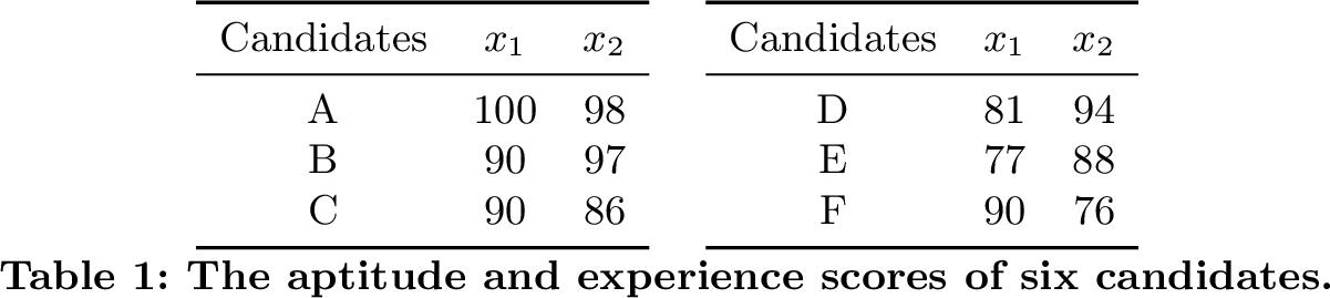 .
.
The ranking regions of these candidates are illustrated in the right panel of Figure 3. Consider the ranking \(A>B>C>D>E>F\), which corresponds to the thin region in the middle of the figure. Under exact stability, this ranking is unstable because its own region has small volume. However, the neighboring regions do not drastically change the rankings. Moving the weights to one side gives \(A>B>D>C>E>F\), which preserves the top two candidates and only swaps \(C\) and \(D\). Moving the weights to the other side gives \(A>B>C>D>F>E\), which preserves the first four candidates and only swaps the last two. These perturbations are different from an unstable case where a small change replaces the leading candidate or substantially rearranges the top of the list.
![Figure 3: Ranking regions for the motivating examples. Left: Example [Example:1], where A>B>C occupies a relatively large region. Right: Example [Example:2], where A>B>C>D>E>F has a small exact region but is adjacent to rankings that preserve the main conclusions.](/article/2607.01546/_pdflatex/jrwgeqap.png "fig:")
Large changes under small weight perturbations indicate fragility and may make the chosen weights appear cherry-picked. Small changes, however, can still support a reliable conclusion if much of the nearby weight space induces rankings that are not too dissimilar.
From Exact Stability to General Stability. The examples above motivate replacing exact stability with a similarity-aware measure. We introduce general stability, a distance-based generalization. Instead of measuring the volume of only the target region, general stability also incorporates the volumes of regions that induce rankings close to the target, with each region weighted according to a user-defined similarity metric.
The similarity metric should be specified depending on which ranking changes matter in the application. For example, a user may care mostly about preserving the top-ranked items, or may want to distinguish a small local swap from a large rearrangement of the ranking. Different choices of similarity metrics encode these judgments. If we assign distance \(0\) to identical rankings and \(\infty\) to all other rankings, general stability reduces to exact stability.
Stability as a Robustness Measure. It is important to clarify how stability should be interpreted. Stability is a robustness measure for a given ranking, not an objective that determines which ranking is best. A highly stable ranking is not necessarily the most appropriate ranking for an application; it only means that the ranking is not sensitive to reasonable changes in the weights. Therefore, the algorithmic task in this paper is to evaluate the robustness of a reported or user-specified ranking by computing its stability score, rather than optimizing over rankings to maximize stability.
Computing Stability. This computation is challenging, especially in high dimensions, because it involves estimating the volumes of multiple high-dimensional ranking regions. Prior work provides exact-stability algorithms in two dimensions and a randomized sampling method for higher dimensions [1]; we extend this computational framework to general stability.
Despite using this sampling-based algorithm, the computational complexity of computing exact stability and general stability can still grow quickly under a fixed error tolerance. The sampling method can be efficient when the stability value is moderate, but it becomes a rare-event estimator when the relevant region has very small volume. Furthermore, general stability may require accounting for many rankings near the target ranking, which can further increase the cost.
Conv-SC. To address this computation problem, we propose a novel algorithm named Conv-SC, which leverages a Markov Chain Monte Carlo (MCMC) sampling technique known as the hit-and-run method [2], [3]. Conv-SC is not a general-purpose solution for every distance function. Rather, it applies to distance functions satisfying a property we term quasiconvexity; this class includes the \(0/\infty\) distance that induces exact stability and the first differing position distance discussed later in the paper.
The key insight behind Conv-SC is that, although computing the volume of a general region in high-dimensional space is \(\#P\)-hard [4], efficient randomized algorithms exist for approximating the volume of convex bodies in polynomial time [5], [6]. However, these algorithms require the region of interest to be convex. In general cases, applying these polynomial-time algorithms is challenging due to the lack of convexity.
By identifying the notion of quasiconvexity for distance functions, we prove that if a distance function is quasiconvex, then the union of all ranking regions within a given distance forms a convex set. This key property enables us to recast the stability computation problem as the computation of convex volumes, which can be efficiently approximated in polynomial time using existing randomized algorithms.
For this restricted class of distance functions, Conv-SC offers a route to polynomial-time stability computation through convex-volume approximation. It is not meant to replace the general sampler in all settings; rather, it addresses the complementary structured regime where the relevant stability sets are convex and sampling may be slowed by small-volume events. Section 6 formalizes quasiconvexity and gives examples.
Summary of Our Contributions↩︎
Our main contributions are as follows:
We introduce and formalize the concept of general stability for rankings, which incorporates user-defined distance functions into stability analysis. The stability of a ranking includes contributions from neighboring similar rankings.
We study practical distance functions that distinguish small ranking changes from large ones and allow users to specify which parts of the ranking matter most.
We extend prior exact-stability computation methods [1] to general stability, including both two-dimensional region enumeration and multidimensional sampling.
We propose a novel algorithm, Conv-SC, for stability computation with quasiconvex distance functions. Quasiconvexity turns the set of weight vectors that induce rankings close to the target into a convex body. Although estimating the volume of a general body is hard, volumes of convex bodies can be approximated efficiently, and Conv-SC exploits this structure in cases where direct sampling becomes a rare-event computation.
We experimentally evaluate general stability on synthetic and real datasets, showing that distance-based stability can distinguish rankings that exact stability treats identically and identify real cases where exact stability is small while general stability remains high. We also compare Conv-SC with sampling under a fixed accuracy target, showing that Conv-SC can be faster for small exact-stability regions.
2 Problem Setup↩︎
2.1 Preliminaries↩︎
We consider a database \(\mathcal{D} = \{t_1, t_2, \ldots, t_n\}\) of \(n\) items. Each item \(t_i \in \mathcal{D}\) is described by a vector of \(d\) scoring attributes: \[t_i = \langle t_i[1],\;t_i[2],\;\ldots,\;t_i[d] \rangle .\] Without loss of generality, these attributes are assumed to lie in \([0,1]\) and are standardized to have equal variance.
A ranking \(\mathfrak{r}\) is a bijective mapping from \(\mathcal{D}\) to \(\{1, 2, \ldots, n\}\). \(\mathfrak{r}(t_i)\) indicates the rank of \(t_i\), and \(\mathfrak{r}^{-1}(k)\) denotes the item in the \(k\)-th position. We focus on rankings induced by linear scoring functions.
A linear scoring function is a mapping \(f_{\mathbf{w}} : \mathbb{R}^d \to \mathbb{R}\) defined by \[f_{\mathbf{w}}(t) \;=\; \sum_{i=1}^d w_i\, t[i],\] where \(\mathbf{w} = \langle w_1, w_2, \ldots, w_d\rangle\) has \(w_i \geq 0\) for all \(i\) and \(\|\mathbf{w}\|_2\le 1\). Equivalently, \(\mathbf{w}\) lies in the positive orthant of the closed unit ball in \(\mathbb{R}^d\), following the weight-space convention in prior stability work [1]. Since positive rescaling of \(\mathbf{w}\) does not change the induced ranking, this domain should be viewed as a convenient representative of weight directions; other normalizations, such as the simplex \(\|\mathbf{w}\|_1=1\), can be handled by replacing \(\mathcal{W}\) or \(\mathcal{W}^*\). The ranking \(\nabla_{f_{\mathbf{w}}}(\mathcal{D})\) is obtained by ordering the items in \(\mathcal{D}\) in descending order of their scores \(f_{\mathbf{w}}(t)\).
Let \(\mathcal{W}\) be the set of all feasible weight vectors. For a ranking \(\mathfrak{r}\) of \(\mathcal{D}\), we denote the set of weight vectors that yield \(\mathfrak{r}\) as: \[\mathcal{R}_{\mathcal{D}}(\mathfrak{r}) \;=\; \bigl\{\, \mathbf{w} \in \mathcal{W} \,\big|\; \nabla_{f_{\mathbf{w}}}(\mathcal{D}) = \mathfrak{r} \bigr\}.\]
2.2 Ranking Regions↩︎
For most choices of \(\mathbf{w}\), no two items receive exactly the same score, and \(\mathbf{w}\) induces a unique ranking. As \(\mathbf{w}\) varies over \(\mathcal{W}\), all weight vectors that produce the same ranking naturally form a ranking region. The exceptional weight vectors that create ties lie on the boundaries between ranking regions. These boundaries are contained in finitely many hyperplanes and have measure zero under the continuous weight-space measures considered here, so adding or removing boundary points does not change any stability value; implementations may break ties arbitrarily.
We now examine the geometry of these ranking regions. First, consider the 2D example from Example [Example:1]. There, \(\mathcal{W}\) (the unit quarter disk) is divided into sectors by rays through the origin, each sector corresponding to a unique ranking. Our goal is to generalize this observation to higher dimensions.
For any pair of items \(t_i, t_j \in \mathcal{D}\), item \(t_i\) ranks before \(t_j\) under the ranking induced by \(f_{\mathbf{w}}\) if and only if \(f_{\mathbf{w}}(t_i) > f_{\mathbf{w}}(t_j)\), which is equivalent to \[\sum_{k=1}^d w_k \left( t_i[k] - t_j[k] \right) > 0.\] The corresponding equality defines a hyperplane through the origin; its two half-spaces determine which of \(t_i\) and \(t_j\) is ranked first.
Therefore, each ranking region is a \(d\)-dimensional cone-like region formed by the intersection of the positive orthant of the closed unit ball with the finite number of half-spaces defined by these hyperplanes for all pairs of items in \(\mathcal{D}\).
2.3 The Stability of a Ranking↩︎
The stability of a ranking is the volume of its ranking region divided by the volume of the positive orthant of the closed unit ball.
Let \(\mathfrak{r}\) be a ranking on \(\mathcal{D}\). Then the stability of \(\mathfrak{r}\) at \(\mathcal{D}\) is \[Stab_{\mathcal{D}}(\mathfrak{r}) = \frac{Vol(\mathcal{R}_{\mathcal{D}}(\mathfrak{r}))}{Vol(\mathcal{W})}\]
In some situations, the user might want to set up an acceptable region \(\mathcal{W}^* \subset \mathcal{W}\), which represents the set of weight vectors considered acceptable for the application. In such cases, the definition of stability could be modified to \[Stab_{\mathcal{D}}(\mathfrak{r}) = \frac{Vol(\mathcal{R}_{\mathcal{D}}^*(\mathfrak{r}))}{Vol(\mathcal{W}^*)}\] where \(\mathcal{R}_{\mathcal{D}}^*(\mathfrak{r}) = \mathcal{R}_{\mathcal{D}}(\mathfrak{r}) \cap \mathcal{W}^*\)
2.4 The General Stability of a Ranking↩︎
Let \(\mathfrak{R}_{\mathcal{D}}\) denote the set of all possible rankings generated by linear scoring functions on the database \(\mathcal{D}\). Then, we can define a distance function on \(\mathfrak{R}_{\mathcal{D}}\), which measures the dissimilarity of rankings. The distance function \(dist\) quantifies the dissimilarity between two rankings. Specifically, a larger value of \(dist(\mathfrak{r}_1, \mathfrak{r}_2)\) indicates a greater degree of difference between the rankings \(\mathfrak{r}_1\) and \(\mathfrak{r}_2\). In this paper, we require the distance function to satisfy two properties, as illustrated in the definition below. (Note that these properties are not enough to make \(dist\) a metric: we do not require the triangle inequality, and two distinct rankings may have distance \(0\).)
A distance function for rankings on \(\mathcal{D}\) is a function \(dist: \mathfrak{R}_{\mathcal{D}} \times \mathfrak{R}_{\mathcal{D}} \to \mathbb{R} \cup \{+\infty\}\), which satisfies the following properties:
For any \(\mathfrak{r} \in \mathfrak{R}_{\mathcal{D}}\), \(dist(\mathfrak{r}, \mathfrak{r}) = 0\)
For any \(\mathfrak{r}_1, \mathfrak{r}_2 \in \mathfrak{R}_{\mathcal{D}}\), \(dist(\mathfrak{r}_1, \mathfrak{r}_2) = dist(\mathfrak{r}_2, \mathfrak{r}_1) \geq 0\)
Then, we define the general stability of a ranking \(\mathfrak{r}_0\) at \(\mathcal{D}\) with a distance function \(dist\) as follows: Let \(\mathfrak{r}_0\) be a ranking on \(\mathcal{D}\). Then the general stability of \(\mathfrak{r}_0\) at \(\mathcal{D}\) with respect to \(dist\) is \[Stab_{\mathcal{D}, dist}(\mathfrak{r}_0) = \frac{1}{Vol(\mathcal{W})}\sum_{\mathfrak{r} \in \mathfrak{R}_{\mathcal{D}}}Vol(\mathcal{R}_{\mathcal{D}}(\mathfrak{r}))exp(-dist(\mathfrak{r}_0, \mathfrak{r}))\] where \(dist\) is a distance function defined by the user.
The user might want to set up an acceptable region \(\mathcal{W}^* \subset \mathcal{W}\). Then, for each ranking \(\mathfrak{r}\), we define \(\mathcal{R}^*_{\mathcal{D}}(\mathfrak{r}) = \mathcal{R}_{\mathcal{D}}(\mathfrak{r}) \cap \mathcal{W}^*\) and let \(\mathfrak{R}^*_{\mathcal{D}}\) denote the set of all possible rankings generated by linear scoring functions with weights in \(\mathcal{W}^*\). Then, the definition of general stability could be modified to \[Stab_{\mathcal{D}, dist}(\mathfrak{r}_0) = \frac{1}{Vol(\mathcal{W}^*)}\sum_{\mathfrak{r} \in \mathfrak{R}^*_{\mathcal{D}} }Vol(\mathcal{R}^*_{\mathcal{D}}(\mathfrak{r}))exp(-dist(\mathfrak{r}_0, \mathfrak{r}))\] This slightly overloads the notation \(Stab_{\mathcal{D}, dist}\); when the acceptable region is relevant, it is assumed to be clear from context.
The idea is straightforward: in evaluating the general stability of a ranking, we do not just look at the volume of its own region in weight space. Rather, we take into account the volumes of all rankings in the acceptable region \(\mathcal{W}^*\). Specifically, we compute the weighted sum of the volumes of all ranking regions, where the weights decrease exponentially as the distances between the ranking of interest and other rankings increase. The definition guarantees that the weight of the volume of the ranking of interest itself is 1, and the farther a ranking is from the ranking of interest, the less impact it will have on the general stability of the ranking of interest.
Consider the following example:
Suppose we have four possible rankings denoted as \(\mathfrak{r}_0\), \(\mathfrak{r}_1\), \(\mathfrak{r}_2\), \(\mathfrak{r}_3\) in an acceptable region \(\mathcal{W}^*\), where \(Vol(\mathcal{W}^*) = 10\). The volumes of the regions corresponding to these four rankings are 2, 3, 3, and 2, respectively. Additionally, \(dist(\mathfrak{r}_0, \mathfrak{r}_1) = dist(\mathfrak{r}_0, \mathfrak{r}_2) = 1\), \(dist(\mathfrak{r}_1, \mathfrak{r}_3) = dist(\mathfrak{r}_2, \mathfrak{r}_3) = 4\), and \(dist(\mathfrak{r}_0, \mathfrak{r}_3) = 5\). Figure 4 presents the rankings and their distances as a graph.
![Figure 4: Graph representation of the rankings and distances in Example [example:general95stability].](/article/2607.01546/_pdflatex/rdxvgnzc.png "fig:")
If we adhere to the conventional stability definition, we find the stability values for both \(\mathfrak{r}_0\) and \(\mathfrak{r}_3\) are \(0.2\). This is not ideal, according to our discussion in the introduction section.
Nevertheless, the general stability of \(\mathfrak{r}_0\) and \(\mathfrak{r}_3\) varies significantly, according to the definition, \(Stab_{\mathcal{D}, dist}(\mathfrak{r}_0) = 0.2 + 0.6e^{-1} + 0.2e^{-5} = 0.4221\) while \(Stab_{\mathcal{D}, dist}(\mathfrak{r}_3) = 0.2 + 0.6e^{-4} + 0.2e^{-5} = 0.2123\). This difference in general stability aligns with our discussion in the introduction section. We can notice that \(\mathfrak{r}_0\) is in proximity to two rankings with considerable ranking regions, but \(\mathfrak{r}_3\) is far from those two rankings, so it is reasonable to consider \(\mathfrak{r}_0\) as more stable than \(\mathfrak{r}_3\).
2.4.1 Stability is Just a Special Case of General Stability↩︎
Consider a simple distance function defined as follows. The \(0/\infty\) distance function \(dist_{0/\infty}\) is a distance function between rankings such that for any \(\mathfrak{r}_1, \mathfrak{r}_2 \in \mathfrak{R}_{\mathcal{D}}\), \[dist_{0/\infty}(\mathfrak{r}_1, \mathfrak{r}_2)= \begin{cases} 0, & \text{if } \mathfrak{r}_1 = \mathfrak{r}_2\\ +\infty& \text{if } \mathfrak{r}_1 \neq \mathfrak{r}_2 \end{cases}\]
It is easy to check that \(dist_{0/\infty}\) satisfies the properties listed in Definition [def:3]. With this distance function, the general stability \(Stab_{\mathcal{D}, dist}\) reduces to the exact stability defined in [1].
2.4.2 Why exponential function?↩︎
We utilize \(exp(-dist(\mathfrak{r}_0, \mathfrak{r}))\) as weights for volumes of ranking regions in Definition [def:4] and [def:5]. This approach elegantly ensures that the weight of the volume of the ranking of interest itself is 1, so that exact stability as defined in [1] is just a special case of the general stability. The exponential form should be interpreted as a monotone similarity kernel: the scale of \(dist\) controls how quickly credit decays as rankings become less similar. It is important to note that users have the flexibility to define their own distance function. If a user prefers not to have weights decrease exponentially with distance, they can manually incorporate a log function into their original distance function.
2.5 The Algorithmic Problem - Stability Computation↩︎
We refer to the task of computing the stability value of a given ranking as stability computation. This task is called stability verification in prior work [1]; we use the term computation to emphasize that the output is a stability score rather than a binary certificate.
Given a dataset \(\mathcal{D}\) with \(n\) items over \(d\) scoring attributes, an acceptable region \(\mathcal{W}^* \subset \mathcal{W}\), a ranking \(\mathfrak{r}\) of \(\mathcal{D}\), and a distance function \(dist\), compute the general stability \(Stab_{\mathcal{D}, dist}(\mathfrak{r})\).
3 Practical Distance Functions↩︎
In Section 1, we argued that exact stability can be too blunt because it treats all non-identical rankings as equally different. General stability addresses this issue by incorporating a user-defined distance between rankings into stability computation.
However, merely defining general stability is not enough. The distance function must reflect which ranking changes matter in the application. For example, the \(0/\infty\) distance function reduces general stability to exact stability and therefore preserves the same exact-match behavior. In this section, we introduce several practical distance functions for rankings.
3.1 Desirable Properties of Distance Functions↩︎
An effective distance function for ranking should satisfy certain properties. First, it should provide meaningful measurements of the differences between rankings, offering a spectrum of distance values rather than a binary distinction. This allows for nuanced assessments of similarity, acknowledging that rankings can be similar to varying degrees. Second, discrepancies at higher ranks should be weighted more heavily than those at lower ranks, reflecting the greater importance often associated with top-ranked items. For example, shifts in the top 10 universities are more impactful than changes among those ranked beyond 100.
3.2 First Differing Position Distance↩︎
Based on these criteria, we first propose a simple distance function: the first differing position distance, denoted as \(dist_{pos}\). This function assigns smaller distances to rankings that agree on more top-ranked items, capturing that early agreements matter more.
Definition 1 (First Differing Position Distance). Given two rankings \(\mathfrak{r}_1\) and \(\mathfrak{r}_2\) over \(n\) items, let \[k = \min \{ i \mid \mathfrak{r}_1^{-1}(i) \neq \mathfrak{r}_2^{-1}(i) \}\] when the two rankings are not identical. The distance \(dist_{pos}\) is defined as: \[dist_{pos}(\mathfrak{r}_1, \mathfrak{r}_2) = \begin{cases} 0, & \text{if } \mathfrak{r}_1 = \mathfrak{r}_2,\\ \frac{1}{k}, & \text{otherwise.} \end{cases}\]
For example, consider the rankings \(\mathfrak{r}_1 = (a, b, c, d, e, f)\) and \(\mathfrak{r}_2 = (a, b, c, f, d, e)\). The first three positions are identical in both rankings. The first difference occurs at position \(4\), where \(\mathfrak{r}_1^{-1}(4) = d\) and \(\mathfrak{r}_2^{-1}(4) = f\). Applying the distance function: \[dist_{pos}(\mathfrak{r}_1, \mathfrak{r}_2) = \frac{1}{4}.\] Thus, the distance between \(\mathfrak{r}_1\) and \(\mathfrak{r}_2\) is \(1/4\), indicating that they are relatively similar since they agree on the top three items.
While \(dist_{pos}\) captures the significance of early agreements, it has limitations. It considers only the position of the first difference and ignores the extent of later disagreement. Thus, it cannot distinguish between rankings that diverge similarly at the first differing position but have varying degrees of overall dissimilarity.
3.3 Exponentially Position-Weighted Kendall’s Tau and Spearman’s Footrule Distances↩︎
Addressing the limitations of \(dist_{pos}\), we introduce two more sophisticated distance functions: the exponentially position-weighted versions of Kendall’s Tau and Spearman’s Footrule distances. These functions are derived from classical distance functions and provide a more informative and nuanced measure of dissimilarity, as well as satisfy the properties we discussed in Section 3.1.
3.3.1 Classical Kendall’s Tau and Spearman’s Footrule Distances↩︎
Kendall’s Tau and Spearman’s Footrule are established metrics for quantifying the dissimilarity between two rankings. Given two rankings \(\mathfrak{r}_1, \mathfrak{r}_2\) over a set of items \(\mathcal{D}\), the Kendall’s Tau distance counts the number of pairwise disagreements: \[\operatorname{dist}_{K}(\mathfrak{r}_1, \mathfrak{r}_2) = \sum_{\substack{(t_i, t_j) \in \mathcal{D} \times \mathcal{D} \\ \mathfrak{r}_1(t_i) < \mathfrak{r}_1(t_j)}} \mathbf{1}\left[ \mathfrak{r}_2(t_i) > \mathfrak{r}_2(t_j) \right],\] where \(\mathbf{1}[ \cdot ]\) is the indicator function.
The Spearman’s Footrule distance measures the sum of absolute differences in positions: \[\operatorname{dist}_{F}(\mathfrak{r}_1, \mathfrak{r}_2) = \sum_{t \in \mathcal{D}} \left| \mathfrak{r}_1(t) - \mathfrak{r}_2(t) \right|.\]
3.3.2 Position Weights↩︎
While Kendall’s Tau and Spearman’s Footrule distances effectively capture overall dissimilarity, they treat discrepancies at all ranks equally. To emphasize discrepancies at higher ranks, [7] introduced position-weighted versions of Kendall’s Tau and Spearman’s Footrule distances. These distances assign weights to each rank position, allowing higher ranks to contribute more to the overall distance.
Definition 2 (Position-Weighted Kendall’s Tau and Spearman’s Footrule Distance [7]). Let \(\Delta = (\delta_1, \delta_2, \dotsc, \delta_n)\) be a sequence of non-increasing weights with \(1 = \delta_1 \geq \delta_2 \geq \dotsb \geq \delta_n \geq 0\). Define the cumulative weight function \(p(i) = \sum_{k=1}^i \delta_k\). For each item \(t_i\), set \[\bar{p}(t_i) = \frac{p\big(\mathfrak{r}_1(t_i)\big) - p\big(\mathfrak{r}_2(t_i)\big)}{\mathfrak{r}_1(t_i) - \mathfrak{r}_2(t_i)}.\] When \(\mathfrak{r}_1(t_i)=\mathfrak{r}_2(t_i)\), we use the convention \(\bar{p}(t_i)=\delta_{\mathfrak{r}_1(t_i)}\). Then, the position-weighted Kendall’s Tau distance* is defined as \[\operatorname{dist}_{K_\Delta}(\mathfrak{r}_1, \mathfrak{r}_2) = \sum_{\substack{(t_i, t_j) \in \mathcal{D} \\ \mathfrak{r}_1(t_i) < \mathfrak{r}_1(t_j)}} \bar{p}(t_i) \bar{p}(t_j) \cdot \left[ \mathfrak{r}_2(t_i) > \mathfrak{r}_2(t_j) \right].\] The position-weighted Spearman’s Footrule distance is defined as \[\operatorname{dist}_{F_\Delta}(\mathfrak{r}_1, \mathfrak{r}_2) = \sum_{i=1}^n \bar{p}(t_i) \left| \sum_{j=1}^{\mathfrak{r}_1(t_i)} \bar{p}\big( \mathfrak{r}_1^{-1}(j) \big) - \sum_{j=1}^{\mathfrak{r}_2(t_i)} \bar{p}\big( \mathfrak{r}_2^{-1}(j) \big) \right|.\]*
3.3.3 Exponential Position Weights↩︎
A remaining issue is the choice of the weight sequence \(\Delta\). To naturally emphasize higher ranks, we propose using exponentially decreasing weights: \[\delta_k = \delta^{k-1}, \quad \text{for } k = 1, 2, \dotsc, n,\] where \(0 < \delta < 1\). This choice yields the weight vector \((1, \delta, \delta^2, \dotsc)\), ensuring that each subsequent position receives exponentially less weight. In the later parts of this paper, we use the notation \(K_\delta\) or \(F_\delta\) to denote the position-weighted Kendall’s Tau/Spearman Footrule distance with exponential weight \((1, \delta, \delta^2, ...)\). For example, \(K_{0.5}\) denotes the position-weighted Kendall’s Tau distance with weight vector \((1, 0.5, 0.25, ...)\). These exponentially weighted distance functions effectively capture the significance of top ranks and account for partial similarities between rankings.
3.4 Other Distance Functions↩︎
It is also important to note that users are not restricted to the distance functions discussed above. There could be other useful distance functions that meaningfully measure differences between rankings. The stability-computation algorithms in the following sections are compatible with any distance function that satisfies Definition [def:3]. Therefore, users can design their own distance functions to suit their specific needs.
4 2D Stability Computation↩︎
Like [1], we first consider the special case \(d = 2\), where the scoring function has the form \[f_{\vec{w}}(t) = w_1t[1] + w_2t[2]\]
The direction of a weight vector can be represented by one angle. We use the convention \[\theta = \arctan(w_1/w_2),\] so \(\theta = 0\) corresponds to ranking only by the second attribute and \(\theta = \pi/2\) corresponds to ranking only by the first attribute. Under this convention, the acceptable region \(\mathcal{W}^*\) is an angular interval \([\theta_{\min}, \theta_{\max}]\).
In 2D, ordering exchanges partition the angular space into intervals, and all weights in one interval induce the same ranking [1]. For general stability, we sweep these intervals and add each interval’s angular width with weight \(\exp(-dist(\mathfrak{r}_0,\mathfrak{r}))\). For a pair of items \((t_i,t_j)\), the exchange angle is determined by \[w_1 \left( t_i[1] - t_j[1] \right) + w_2 \left( t_i[2] - t_j[2] \right) = 0.\]
Equivalently, for each pair we compute \[a_{(i,j)} = \frac{t_j[2] - t_i[2]}{t_i[1] - t_j[1]}, \quad b_{(i,j)} = t_i[1] - t_j[1].\] The list \(L\) of all such tuples has size \(\Theta(n^2)\). Sorting \(L\) orders the exchange angles, and the sweep in Algorithm 5 accumulates the weighted contribution of each interval.
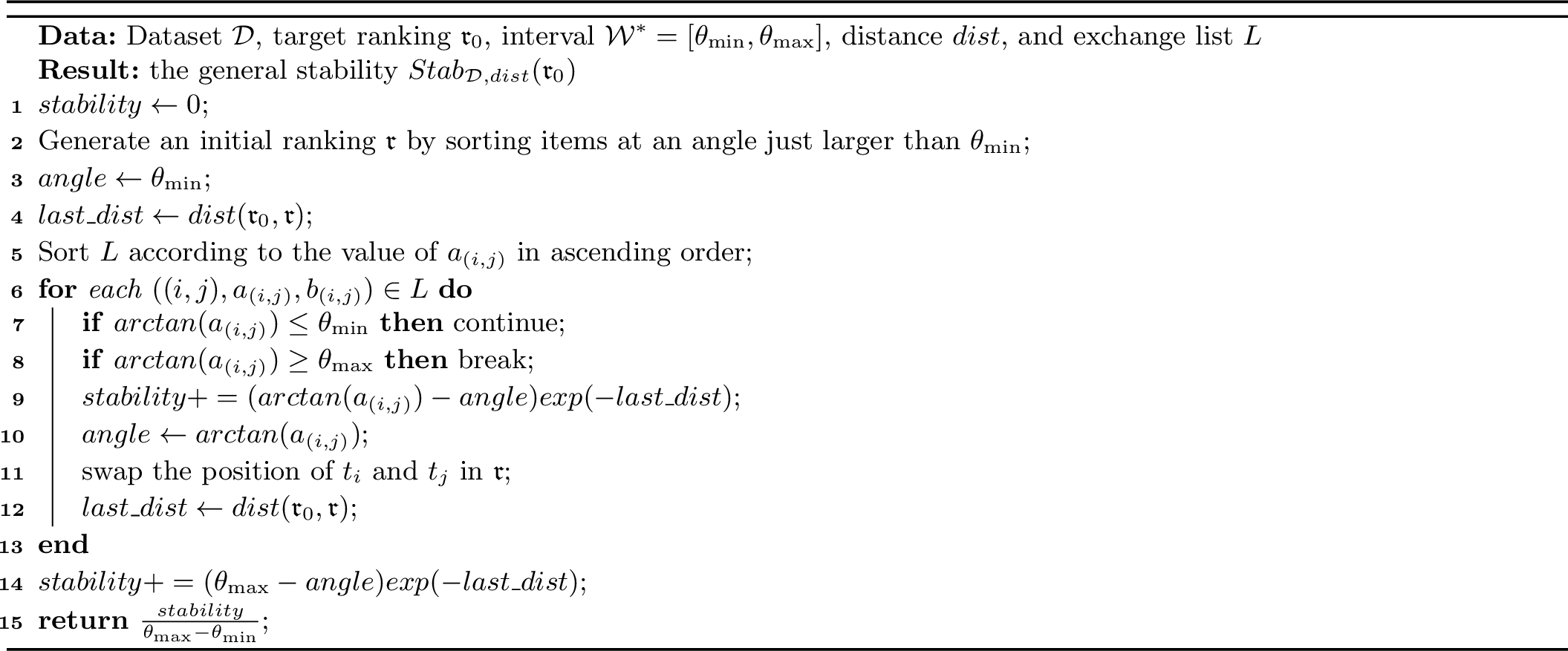
Generating the initial rank takes \(\Theta(n \log n)\), and sorting \(L\) takes \(\Theta(n^2 \log n)\). The main for loop in \(GSC_{2d}\) runs for \(\Theta(n^2)\) iterations. Assuming \(dist\) takes \(D\) time to compute, the total time complexity of \(GSC_{2d}\) is \(O(n^2(D + \log n))\).
5 Multidimensional Stability Computation↩︎
When dealing with general distance functions, we can extend the stability-computation algorithms proposed by [1]. As we discussed in Section 2.2, each ranking region is a \(d\)-dimensional cone-like region whose boundary is determined by pairwise comparison hyperplanes. Since accurately calculating the volumes of high-dimensional polyhedra is \(\#P\)-hard [4], [1] employs Monte-Carlo methods to approximate the stability of a target ranking. We extend their method to make it suitable for general stability.
5.1 An Unbiased Sampler on \(\mathcal{W}^*\)↩︎
To estimate the volumes of the truncated cone-like ranking regions inside \(\mathcal{W}^*\) using rejection sampling, we need samples of weights from \(\mathcal{W}^*\). These samples must be unbiased, i.e., the probability that a sample falls into each ranking region is proportional to the volume of that region. Formally, for each \(\mathfrak{r} \in \mathfrak{R}_{\mathcal{D}}\), an unbiased sample \(W\) should satisfy: \[P(W \in \mathcal{R}^*_{\mathcal{D}}(\mathfrak{r})) = \frac{Vol(\mathcal{R}^*_{\mathcal{D}}(\mathfrak{r}))}{Vol(\mathcal{W}^*)}\]
An unbiased sampler satisfying this property was proposed in [1]. It generates samples from \(\mathcal{W}^*\) in time linear in the dimension. We will directly adopt their sampler in our method.
5.2 Stability Computation↩︎
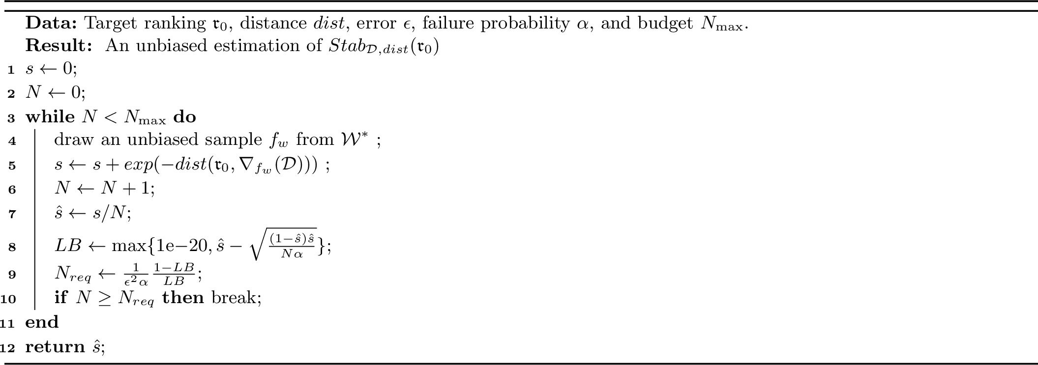
The \(GSC_{md}\) algorithm described in Algorithm 6 is a direct extension of the stability oracle described in [1]. It offers an unbiased estimation of the general stability of a given target ranking \(\mathfrak{r}_0\) based on a fixed number of unbiased samples taken from \(\mathcal{W}^*\).
Let \(D_{dist}(n,d)\) denote the time needed to evaluate the contribution of one sampled weight for the chosen distance function \(dist\), including any ranking information required for that evaluation. This cost is distance-dependent. For distances such as \(dist_{0/\infty}\), one may only need to test whether the sampled weight preserves the target ranking, which can avoid constructing a complete sorted ranking. For other distances, such as Kendall’s tau or Spearman’s footrule, evaluating the contribution may require computing a full induced ranking. In the following analysis, \(D_{dist}(n,d)\) abstracts this per-sample evaluation cost.

The estimator is unbiased because each sample falls in a ranking region with probability equal to that region’s volume fraction in \(\mathcal{W}^*\). Therefore, \[E[\hat{s}] = \sum_{\mathfrak{r} \in \mathfrak{R}_{\mathcal{D}} } \frac{Vol(\mathcal{R}^*_{\mathcal{D}}(\mathfrak{r}))}{Vol(\mathcal{W}^*)} exp(-dist(\mathfrak{r}_0, \mathfrak{r})) = Stab_{\mathcal{D}, dist}(\mathfrak{r}_0).\]
When taking \(dist_{0/\infty}\) as the distance function, \(GSC_{md}\) will be equivalent to stability oracle \(S\) proposed in [1].
5.3 \(GSC_{md}\) with Fixed Error and Failure Probability↩︎
The \(GSC_{md}\) algorithm inherently involves a trade-off between computational time and accuracy. As more samples are drawn from \(\mathcal{W}^*\), the estimate \(\hat{s}\) becomes more accurate; however, the computational time increases proportionally, since \(GSC_{md}\) runs in \(O(ND_{dist}(n,d))\) time under the per-sample cost notation above. In practice, users often specify an allowable error threshold \(\epsilon\) and a failure probability \(\alpha\), expecting the algorithm to produce an estimate within \((1 \pm \epsilon)s\) of the true value \(s = Stab_{\mathcal{D}, \, dist}(\mathfrak{r}_0)\) with probability at least \(1 - \alpha\).
In this subsection, we analyze the time-accuracy trade-off in \(GSC_{md}\), introduce a method to run \(GSC_{md}\) with fixed error and failure probability, and examine its sample complexity. Since the total runtime is obtained by multiplying the sample budget by \(D_{dist}(n,d)\), exponential sample complexity immediately yields exponential runtime up to this per-sample evaluation factor.
5.3.1 Sample Size↩︎
To achieve an \(\epsilon\)-approximation of \(s\) with failure probability at most \(\alpha\), we need to determine the minimum sample size \(N\) such that:
\[P\left( |\hat{s} - s| < \epsilon s \right) \geq 1 - \alpha.\]
5.3.1.1 Special Case: \(dist_{0/\infty}\)
When using \(dist_{0/\infty}\), \(\hat{s}\) follows a binomial distribution \(\operatorname{Binomial}(N, s)\). The normal approximation to the binomial distribution allows us to estimate the required sample size:
\[N = \left( \dfrac{z_{\alpha/2}}{\epsilon} \right)^2 \dfrac{1 - s}{s},\]
This special case shows that, for the class of distance functions considered in this paper, there exist valid inputs for which estimating \(s\) to a fixed relative error requires a sample budget proportional to \((1-s)/s\), up to constants depending on \(\epsilon\) and \(\alpha\).
5.3.1.2 General Case
For a general distance function, let one sample contribution be \[X=\exp(-dist(\mathfrak{r}_0,\nabla_{f_W}(\mathcal{D}))).\] Since \(0\leq X\leq 1\) and \(E[X]=s\), we have \(E[X^2]\leq E[X]=s\), so \[\operatorname{Var}[\hat{s}] \leq \frac{s-s^2}{N}.\] Applying Chebyshev’s inequality, we find:
\[P\left( | \hat{s} - s | \geq \epsilon s \right) \leq \frac{ \operatorname{Var}[\hat{s}] }{ \epsilon^2 s^2 } \leq \frac{ (1 - s) }{ N \epsilon^2 s }\] Thus, to ensure \(P\left( | \hat{s} - s | \geq \epsilon s \right) \leq \alpha\), it suffices to have
\[N = \frac{ (1 - s) }{ \alpha \epsilon^2 s }\]
5.3.2 Time and Accuracy↩︎
The special case of \(dist_{0/\infty}\) gives a lower-bound witness: the sample budget can be as large as a constant multiple of \(\frac{1-s}{s}\) for fixed \(\epsilon\) and \(\alpha\). The general variance bound gives the matching upper bound: for every distance function considered here, it suffices to take a sample budget at most a constant multiple of \(\frac{1-s}{s}\) for fixed \(\epsilon\) and \(\alpha\).
Therefore, the worst-case sample complexity of \(GSC_{md}\), over the admissible distance functions in this framework, is \[N = \Theta \left( \dfrac{ 1 - s }{ s } \right),\] with constants depending on \(\epsilon\) and \(\alpha\). This does not mean that every distance function or dataset requires many samples; when the stability value is moderate, \(GSC_{md}\) can be very efficient in practice. The bound identifies the complementary rare-event regime: as \(s\) gets smaller, fixed error and failure guarantees need more samples.
5.3.3 Run \(GSC_{md}\) with Fixed Error and Failure Probability↩︎
The sample bound above depends on the unknown stability value \(s\). In practice, we use an adaptive implementation that updates the estimate after each sample, forms an empirical lower bound \(LB\) on \(s\), and then substitutes \(LB\) into the sufficient sample-size bound. This gives the stopping rule in Algorithm 7. The rule is conservative when \(LB\) is below the true stability value; if the maximum sample budget is reached first, the algorithm returns the current estimate.
5.3.4 Why \(GSC_{md}\) is Not Polynomial↩︎
We now use the sample-complexity bound above to explain why \(GSC_{md}\) is not polynomial in the worst case when the dimension \(d\) is part of the input. The key point is that the sample budget depends on \((1-s)/s\). Thus, it is enough to show that there are valid inputs for which the target stability \(s\) is exponentially small in \(d\).
We prove this using the special case \(dist_{0/\infty}\). Under this distance, \(GSC_{md}\) estimates exact stability: a sample contributes \(1\) if it induces the target ranking and \(0\) otherwise. Therefore, the stability of a ranking is the volume fraction of its own ranking region in \(\mathcal{W}^*\).
For every fixed dimension \(d\), there exist databases \(\mathcal{D}\) with \(n\) tuples in \(d\) dimensions whose positive weight space contains \(\Omega(n^{2(d-1)})\) nonempty ranking regions.
Proof. We use Cover’s result on linearly inducible orderings [8]. Let \(Q(n,d)\) be the number of distinct orderings of \(n\) points in general position in \(\mathbb{R}^d\) that can be induced by linear projections \(w \cdot t_i\), as \(w\) ranges over all directions in \(\mathbb{R}^d\). [8] gives the recurrence \[Q(n,d)=Q(n-1,d)+(n-1)Q(n-1,d-1),\] with the base cases \(Q(n,1)=2\) and \(Q(2,d)=2\). This recurrence implies, by induction on \(d\), that for each fixed \(d\), \(Q(n,d)\) is a polynomial in \(n\) of degree \(2(d-1)\). Hence \(Q(n,d)=\Theta(n^{2(d-1)})\) for fixed \(d\).
These projection-induced orderings are exactly the ranking regions generated by the pairwise comparison hyperplanes \[H_{ij}=\{w\in \mathbb{R}^d: w\cdot(t_i-t_j)=0\}.\] On one side of \(H_{ij}\), \(t_i\) has a larger score than \(t_j\); on the other side, \(t_j\) has a larger score than \(t_i\).
The count in [8] is over all directions, while our weight space is the positive orthant of the unit ball. The \(2^d\) coordinate orthants partition the directions in \(\mathbb{R}^d\), so at least one orthant contains a \(1/2^d\) fraction of the ranking regions. By flipping coordinate signs of all tuples if necessary, we may map that orthant to the positive orthant without changing the number of regions inside it. Therefore, for each fixed \(d\), the positive orthant contains \(\Omega(n^{2(d-1)})\) nonempty ranking regions. The hidden constant in this \(\Omega(\cdot)\) notation may depend on \(d\). ◻
Take \(\mathcal{W}^* = \mathcal{W}\). The proposition implies that, for these databases, \(\mathcal{W}\) is partitioned into \(\Omega(n^{2(d-1)})\) nonempty ranking regions. Hence at least one ranking region has volume fraction \[s = O(n^{-2(d-1)}).\] For \(dist_{0/\infty}\), this volume fraction is exactly the stability of the corresponding ranking. Thus, we are not assuming that \(s\) is small for every input; rather, the proposition constructs valid inputs for which at least one target ranking has \[s = O(n^{-2(d-1)}).\] For sufficiently large \(n\), this gives \(s \leq 1/2\), and therefore \((1-s)/s \geq 1/(2s)\). Substituting this constructed small value of \(s\) into the worst-case sample-complexity bound gives \[N = \Theta\left(\frac{1-s}{s}\right) = \Omega(n^{2(d-1)})\] for fixed \(\epsilon\) and \(\alpha\). This lower bound is not polynomial in the combined input parameters \(n\) and \(d\): for any fixed polynomial degree in \(n\), choose \(d\) large enough that \(2(d-1)\) exceeds that degree, and then let \(n\) grow. Thus, when \(d\) is allowed to vary, \(GSC_{md}\) can require non-polynomially many samples. Since the total runtime is the sample budget multiplied by the per-sample evaluation cost \(D_{dist}(n,d)\), the algorithm is not polynomial-time in the worst case under a fixed relative-error guarantee.
6 Polynomial Stability Computation for Quasiconvex Distance Functions↩︎
Both the stability computation method proposed in [1] and the \(GSC_{md}\) we proposed in the last section are sampling-based in multidimensional settings. They are broadly applicable, but under a fixed relative-error guarantee their sample complexity can become large when the stability value is small.
In this section, we propose a novel algorithm, Conv-SC, for this structured rare-event regime. Conv-SC can perform stability computation in polynomial time under fixed error tolerance and failure probability, provided that the distance function satisfies the quasiconvexity requirement and the acceptable region \(\mathcal{W}^*\) is convex. This is a structural restriction on the distance function, not a requirement for general stability itself: distances such as the position-weighted Kendall’s Tau and Spearman’s Footrule distances from Section 3.3 are useful for the general sampling-based methods, but are not quasiconvex in general. Notably, \(dist_{0/\infty}\) satisfies the quasiconvexity requirement.
6.1 Motivation: Efficient Volume Computation of Convex Bodies↩︎
Computing the exact volume of high-dimensional polyhedra is \(\#P\)-hard [4], meaning that no known polynomial-time algorithms exist for this task. However, efficient randomized algorithms can approximate the volume of convex bodies within a fixed error tolerance in polynomial time. Dyer, Frieze, and Kannan [5] first proposed such an algorithm with a fixed error bound. By leveraging the hit-and-run sampling method [2], a Markov chain Monte Carlo technique that uniformly samples points within a convex set, Kannan, Lovász, and Simonovits [6] improved the computation time to \(O^*(d^{5})\), where \(d\) is the number of dimensions, and the “soft-O” notation \(O^*\) suppresses logarithmic factors like \(\log d\) and other parameters such as the error bound \(\epsilon\). The theoretical guarantee assumes access to a randomized convex-volume approximation routine with the stated accuracy guarantee.
A key requirement for applying these algorithms is that the body must be convex. In our context, each ranking region is indeed convex. However, calculating the general stability requires computing the volumes of multiple ranking regions. Since the number of these regions grows exponentially with the number of dimensions, even efficiently approximating each individual volume leads to an overall exponential time complexity.
To overcome this challenge, we propose a novel approach. Instead of computing the volume of each ranking region separately, we group regions based on their distances to the ranking of interest. We then compute the combined volume of all ranking regions that are within a certain distance \(r\) from the ranking of interest.
We introduce the concept of quasiconvexity. If a distance function is quasiconvex, then the union of ranking regions within a distance \(r\) forms a convex set. This property allows us to apply the hit-and-run method to efficiently calculate the general stability. In the following subsections, we will formally define quasiconvexity and present the related algorithms.
6.2 Quasiconvexity of Distance Functions↩︎
A distance function \(dist\) for rankings on \(\mathcal{D}\) is quasiconvex if and only if it satisfies the following property: for any \(w_0,w_1,w_2\in \mathbb{R}^d\) and \(\lambda\in (0, 1)\), \[\begin{align} &dist(\nabla_{f_{\vec{w_0}}}(\mathcal{D}), \nabla_{f_{\overrightarrow{\lambda w_1 + (1-\lambda) w_2}}}(\mathcal{D}) )\\ \leq& \max \{ dist(\nabla_{f_{\vec{w_0}}}(\mathcal{D}), \nabla_{f_{\vec{w_1}}}(\mathcal{D})), dist(\nabla_{f_{\vec{w_0}}}(\mathcal{D}), \nabla_{f_{\vec{w_2}}}(\mathcal{D}))\} \end{align}\]
The reason that we define quasiconvexity is that it exhibits the following important property:
If a distance function \(dist\) is quasiconvex, then for any linearly inducible ranking \(\mathfrak{r}\) and real number \(r\), the closed ball \(B_{dist}(\mathfrak{r}, r) := \{w \in \mathbb{R}^d | dist(\mathfrak{r}, \nabla_{f_{\vec{w}}}(\mathcal{D})) \leq r\}\) is convex.
Proof. For any \(w_1,w_2\in B_{dist}(\mathfrak{r},r)\) and \(0<t<1\), choose \(w_0\) such that \(\mathfrak{r}=\nabla_{f_{\vec{w_0}}}(\mathcal{D})\). By quasiconvexity, \[\begin{align} &dist(\mathfrak{r},\nabla_{f_{\overrightarrow{t w_1+(1-t)w_2}}}(\mathcal{D}))\\ &\qquad \leq \max\{dist(\mathfrak{r},\nabla_{f_{\vec{w_1}}}(\mathcal{D})), dist(\mathfrak{r},\nabla_{f_{\vec{w_2}}}(\mathcal{D}))\}\leq r. \end{align}\] Thus \(t w_1+(1-t)w_2\in B_{dist}(\mathfrak{r},r)\). ◻
6.3 Quasiconvex Distance Functions↩︎
It is easy to check that \(dist_{0/\infty}\) is quasiconvex. Now, we show that the first differing position distance (\(dist_{pos}\)) from Definition 1 is also quasiconvex. These examples illustrate the class targeted by Conv-SC; not all practical ranking distances are quasiconvex.
\(dist_{pos}\) is quasiconvex.
Proof. Let \(w_0,w_1,w_2\in \mathbb{R}^d\) and \(\lambda\in(0,1)\), and let \(\mathfrak{r}_i=\nabla_{f_{w_i}}(\mathcal{D})\) for \(i=0,1,2\). If \(\mathfrak{r}_1=\mathfrak{r}_2=\mathfrak{r}_0\), then all pairwise score inequalities in \(\mathfrak{r}_0\) are preserved by \(\lambda w_1+(1-\lambda)w_2\), so the desired inequality is immediate. Otherwise, let \(k\) be the first position at which either \(\mathfrak{r}_1\) or \(\mathfrak{r}_2\) differs from \(\mathfrak{r}_0\). Then the first \(k-1\) items of all three rankings are the same and in the same order, and \[\frac{1}{k}\leq \max\{dist_{pos}(\mathfrak{r}_0,\mathfrak{r}_1),dist_{pos}(\mathfrak{r}_0,\mathfrak{r}_2)\}.\] Let \(t_m=\mathfrak{r}_0^{-1}(m)\) for \(m<k\). For any \(m<k\) and any item \(x\) outside the first \(m\) positions, both \(w_1\) and \(w_2\) rank \(t_m\) above \(x\). Since score differences are linear in the weight vector, \[(\lambda w_1+(1-\lambda)w_2)\cdot(t_m-x)>0.\] Thus \(\nabla_{f_{\lambda w_1+(1-\lambda)w_2}}(\mathcal{D})\) preserves the first \(k-1\) positions of \(\mathfrak{r}_0\). Its first differing position from \(\mathfrak{r}_0\) is no earlier than \(k\), so \[\begin{align} &dist_{pos}(\mathfrak{r}_0,\nabla_{f_{\lambda w_1+(1-\lambda)w_2}}(\mathcal{D}))\\ &\qquad \leq \frac{1}{k} \leq \max\{dist_{pos}(\mathfrak{r}_0,\mathfrak{r}_1), dist_{pos}(\mathfrak{r}_0,\mathfrak{r}_2)\}. \end{align}\] ◻
6.4 The Conv-SC Algorithm↩︎
We denote the randomized convex-body volume routine by \(\mathbf{V}\). For any convex set \(S\) in \(\mathbb{R}^d\), \(\mathbf{V}(S)\) estimates the volume of \(S\) in \(O^*(d^{5})\) time for fixed accuracy parameters.
Conv-SC is most useful when the quasiconvex distance function has a compact set of relevant distance levels. For example, \(dist_{0/\infty}\) has only two possible values, and \(dist_{pos}\) has one level for each first differing position. For \(dist_{pos}\), the level set for agreement through the first \(k-1\) positions can be written using linear constraints that place each prefix item above every remaining item, yielding \(O(kn)\) ranking constraints at level \(k\). We list the possible values of \(dist\) in increasing order as \(R = \{r_0, r_1, ..., r_k\}\), where \(0=r_0<r_1<\cdots<r_k\). For each level, let \(C_i = B_{dist}(\mathfrak{r}_0, r_i) \cap \mathcal{W}^*\) denote the feasible part of the distance ball.
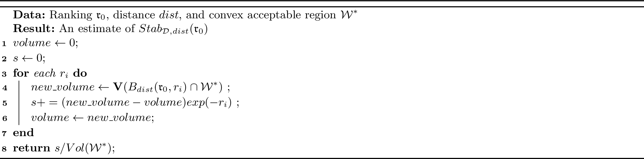
Grouping ranking regions by their distance to \(\mathfrak{r}_0\) gives: \[\begin{align} Stab_{\mathcal{D}, dist}(\mathfrak{r}_0) =& \frac{1}{Vol(\mathcal{W}^*)}\sum_{\mathfrak{r} \in \mathfrak{R}^*_{\mathcal{D}} }Vol(\mathcal{R}^*_{\mathcal{D}}(\mathfrak{r}))exp(-dist(\mathfrak{r}_0, \mathfrak{r})) \\ =&\frac{1}{Vol(\mathcal{W}^*)} \sum_{i=0}^k exp(-r_i) \sum_{\mathfrak{r}, dist(\mathfrak{r}_0, \mathfrak{r}) = r_i} Vol(\mathcal{R}^*_{\mathcal{D}}(\mathfrak{r})) \\ =&\frac{1}{Vol(\mathcal{W}^*)} \Bigl(Vol(C_0) \\ &+ \sum_{i=1}^k exp(-r_i) [Vol(C_i) - Vol(C_{i-1})]\Bigr) \end{align}\]
According to Proposition [prop:1], each \(B_{dist}(\mathfrak{r}_0, r_i)\) is convex. Since \(\mathcal{W}^*\) is also assumed to be convex, each feasible level set \(C_i = B_{dist}(\mathfrak{r}_0, r_i) \cap \mathcal{W}^*\) is convex as well. Therefore, each level-set volume can be approximated in polynomial time for fixed accuracy. The overall cost is polynomial in the dimension for each convex body and scales with the number of distance levels that are evaluated. For distances such as \(dist_{0/\infty}\) and \(dist_{pos}\), this level-set dependence is small enough to make the method practical. The algorithm is shown below in Algorithm 8.
Before calling the volume routine, Conv-SC computes a well-conditioned interior point when the convex body is represented by linear ranking constraints and the unit ball. In the \(0/\infty\) case, this amounts to finding the largest ball centered at \(c\) that remains inside the target ranking region: \[\begin{array}{ll} \text{maximize} & \rho \\ \text{subject to} & c_j \geq \rho \quad \text{for all } j,\\ & c\cdot(t_a-t_b) \geq \rho\|t_a-t_b\|_2 \quad \text{for adjacent } t_a \succ t_b,\\ & \|c\|_2 + \rho \leq 1 . \end{array}\] It is enough to constrain adjacent pairs in the target order: if all adjacent score inequalities hold, then all pairwise inequalities follow by transitivity of the scalar scores. This is a second-order cone program and can be solved in polynomial time by standard interior-point methods [9]. The resulting \(\rho\) gives a certified inner-ball radius for the convex-volume routine.
In practice, constructing the volume oracle requires a strict interior point for each convex body. If this point is too close to the boundary, the inner ball may be tiny and the random walk may mix slowly. The max-margin step above addresses this issue for the \(0/\infty\) distance. For other quasiconvex distances such as \(dist_{pos}\), the same idea applies once the level set is written as linear constraints.
7 Experiments↩︎
We experimentally evaluated both the modeling benefits and the computational costs of general stability. For the former, real-world case studies and minor-swap sensitivity checks showed that exact stability can be misleadingly brittle and that distance-sensitive stability better preserves meaningful ranking similarity. For the latter, we found that the approximation methods achieve practical accuracy and runtime for distance-sensitive stability scores on real datasets. Furthermore, we show that Conv-SC realizes its intended advantage: for convex stability regions, it turns the high-dimensional exact-stability computation into a polynomial-time convex-volume approximation task.
7.1 Experimental Setup and Datasets↩︎
Hardware and platform. The experiments were conducted using an Intel i7-12700F processor, 16 GB memory, running Linux. The algorithms were implemented in C++ 17, and the program was compiled in \(gcc\) with optimization level O3. Conv-SC uses Volesti [10] for convex-body volume approximation.
Datasets. The real-data experiments use eight datasets: QS World University Rankings 2024–2026 [11], Times Higher Education (THE) 2016 [12], Center for World University Rankings (CWUR) 2015 [13], CSMetrics 2016 [14], the 2023 Global Multidimensional Poverty Index (MPI) [15], CSRankings 2024 [16], NBA 2023–24 [17], and the Environmental Performance Index (EPI) 2024 [18]. The numbers of numeric indicators used in our processed tasks are 6 for QS, 5 for THE, 8 for CWUR, 2 for CSMetrics, 10 for MPI, 4 for CSRankings, 5 for NBA, and 6 for EPI. Selected experiments use generated datasets as controls.
7.2 Real-World Ranking Investigation↩︎
General stability was introduced because exact stability only checks whether the entire ranking is reproduced exactly. We therefore ask whether exact stability and distance-sensitive general stability agree on real datasets. For each dataset, we consider top-\(n\) rankings with \(n=10,20,30,50,100\), normalize the selected attributes, and sample target rankings from random positive weights. For each target ranking, exact stability, \(dist_{pos}\) stability, \(K_{0.5}\) stability, and \(F_{0.5}\) stability are estimated from the same random weight samples. Table 1 reports the resulting correlation matrix.
| Score | Exact | \(dist_{pos}\) | \(K_{0.5}\) | \(F_{0.5}\) |
|---|---|---|---|---|
| Exact | 1.000 | 0.391 | 0.288 | 0.275 |
| \(dist_{pos}\) | 0.391 | 1.000 | 0.969 | 0.968 |
| \(K_{0.5}\) | 0.288 | 0.969 | 1.000 | 0.998 |
| \(F_{0.5}\) | 0.275 | 0.968 | 0.998 | 1.000 |
CWUR patents top 30. In this dataset, items are universities and the candidate set consists of the 30 universities with the highest patent score in CWUR. We keep the eight CWUR attributes and use the equal-weight ranking as the target. The target begins with Harvard, MIT, Stanford, Johns Hopkins, and UC Berkeley. Under exact stability, Conv-SC estimates that this full top-30 ordering occupies only about \(6.15\times 10^{-6}\) of the feasible weight space, below the random-weight baseline (\(6.0\times 10^{-5}\)), so the exact score suggests that the ranking is highly fragile. In contrast, the top-sensitive Kendall stability is \(0.9179\), above its baseline of \(0.8856\).
The local perturbation results explain this difference. At perturbation radius \(0.05\), the full ranking is reproduced only \(3.9\%\) of the time. However, the top-5 set is preserved in essentially every sample. Thus, for this case, the instability captured by exact stability comes almost entirely from changes below the leading universities.
This example illustrates why exact stability alone can be too brittle for interpreting real ranked lists. The exact score treats every non-identical ordering as equally different, whereas a suitable distance-sensitive score identifies that the top-ranked items remain stable and that most changes occur lower in the list.
7.3 Sensitivity to Minor Ranking Changes↩︎
As a lightweight check of the same effect across datasets, we take top-10 sampled target rankings, swap one adjacent pair in the lower half, and measure the normalized average change \(\mathbb{E}[|S(\mathfrak{r})-S(\mathfrak{r}')|]/\mathbb{E}[S(\mathfrak{r})]\). Averaged over the eight real datasets, this value is \(0.766\) for exact stability, while the distance-sensitive scores are close to zero: \(8.36{\times}10^{-3}\) for \(dist_{pos}\), \(5.30{\times}10^{-4}\) for \(K_{0.5}\), and \(8.65{\times}10^{-4}\) for \(F_{0.5}\). Thus, exact stability changes substantially under a minor lower-half swap, whereas distance-sensitive scores barely move.
7.4 Error Analysis for \(GSC_{md}\) and Conv-SC↩︎
\(GSC_{md}\) and Conv-SC are approximation methods: they do not return the ground-truth stability value, but an estimate whose accuracy is controlled by a user-specified error tolerance. The theoretical analysis guarantees that, with high probability, the relative error is below the requested tolerance. This guarantee is promising in theory, but it does not show what the approximation error looks like in practice, or how large the observed errors usually are relative to the requested tolerance.
This investigation requires tasks where the ground-truth stability value is known. For general multidimensional inputs this value is unavailable, but in 2D, \(GSC_{2d}\) computes the ground-truth value under the \(0/\infty\) distance. We use these 2D ground-truth values to compare fixed-error \(GSC_{md}\) and Conv-SC estimates. The main check uses requested relative-error tolerance \(\epsilon=0.3\), i.e., 30%, and failure probability \(\alpha=0.1\).
The observed errors are usually much smaller than the requested 30% tolerance, for both generated 2D tasks and real two-attribute projections. Table 2 reports the real-data aggregates. Tightening the requested bound to \(\epsilon=0.05\) on generated 2D tasks further reduced the mean errors to 1.4% for \(GSC_{md}\) and 3.2% for Conv-SC.
| Dataset | \(GSC_{md}\) | Conv-SC | ||||
| Relative error | Avg. | Std. | Max. | Avg. | Std. | Max. |
| MPI | 6.5% | 5.4% | 19.6% | 8.1% | 6.3% | 24.5% |
| CWUR | 6.6% | 4.6% | 16.0% | 5.9% | 4.9% | 19.1% |
| CSMetrics | 2.4% | 2.0% | 5.2% | 2.1% | 1.3% | 3.9% |
| THE | 7.5% | 5.7% | 20.2% | 6.5% | 4.7% | 16.2% |
| QS | 7.3% | 4.2% | 15.9% | 6.9% | 4.0% | 16.3% |
| CSRank. | 6.4% | 3.1% | 10.7% | 8.6% | 6.8% | 21.1% |
| NBA | 6.3% | 2.5% | 9.2% | 12.5% | 9.5% | 26.0% |
| EPI | 7.0% | 5.1% | 23.0% | 8.3% | 7.6% | 24.7% |
| All | 6.6% | 4.9% | 23.0% | 7.5% | 6.3% | 26.0% |
7.5 Efficiency of \(GSC_{2d}\) and \(GSC_{md}\)↩︎
We measure the efficiency of \(GSC_{2d}\) and \(GSC_{md}\) on representative ranking tasks. For \(GSC_{2d}\), we report exact runtimes on two-attribute inputs. For \(GSC_{md}\), we report the sampling cost needed to meet a fixed user-specified error tolerance.
Efficiency of \(GSC_{2d}\). CSMetrics is the natural real-data case for this experiment because its reported ranking is defined by two publication-based scores. We therefore report CSMetrics first. To check that this behavior is not specific to this dataset, we also sample one two-attribute projection from each of the other real datasets and compute exact 2D general stability under \(dist_{pos}\), \(K_{0.5}\), and \(F_{0.5}\). Table 3 shows that all these real 2D cases finish in milliseconds.
| Dataset | Attributes | \(dist_{pos}\) | \(K_{0.5}\) | \(F_{0.5}\) |
|---|---|---|---|---|
| CSMetrics | Measured/Predicted | 4.314 | 47.716 | 10.227 |
| QS | Faculty/Citations | 0.936 | 4.942 | 2.133 |
| THE | Research/Income | 4.539 | 56.388 | 11.438 |
| CWUR | Publications/Faculty | 3.769 | 45.751 | 10.095 |
| MPI | Cooking fuel/Mortality | 4.352 | 40.080 | 8.613 |
| CSRank. | Interdisc./AI | 3.609 | 29.289 | 8.942 |
| NBA | Steals/Blocks | 0.921 | 4.051 | 1.737 |
| EPI | Biodiversity/Water | 4.401 | 52.841 | 10.675 |
Efficiency of \(GSC_{md}\). Following the fixed-error setting in Section 5, we use \(\epsilon=0.3\) and \(\alpha=0.1\). Table 4 reports runtimes on representative real-data tasks with reported or naturally defined target rankings.
| Task | \(dist_{pos}\) | \(K_{0.5}\) | \(F_{0.5}\) | Task | \(dist_{pos}\) | \(K_{0.5}\) | \(F_{0.5}\) |
|---|---|---|---|---|---|---|---|
| QS26 | 4.313 | 0.905 | 1.464 | CWUR | 6.674 | 0.951 | 1.606 |
| QS25 | 4.291 | 0.944 | 1.519 | CSM | 1.956 | 0.472 | 0.488 |
| QS24 | 4.250 | 1.059 | 2.057 | CSR | 2.771 | 0.215 | 0.313 |
| THE | 9.114 | 1.872 | 2.486 | NBA | 3.450 | 0.662 | 1.075 |
The rows in Table 4 finish in at most \(0.010\) seconds. This shows that \(GSC_{md}\) is practical for the distance-sensitive stability scores used in the real-data investigation.
Exact stability can also be measured by \(GSC_{md}\), since it is the special case of general stability under the \(0/\infty\) distance. However, exact-stability values are usually much smaller than the corresponding distance-sensitive scores because every non-identical ranking receives zero credit. Conv-SC is better suited to this setting: it estimates the convex exact-stability region directly, as shown next.
7.6 Polynomial Efficiency of Conv-SC↩︎
Conv-SC is motivated by the gap between exact and approximate volume computation: exact high-dimensional polyhedral volume is \(\#P\)-hard [4], while convex-body volume can be approximated in polynomial time [5], [6]. When the stability region is convex, Conv-SC exploits this advantage directly.
This experiment checks whether the polynomial-time convex-volume advantage of Conv-SC appears in runtime. We compare \(GSC_{md}\) and Conv-SC under the \(0/\infty\) distance, using generated data to observe the trend over multiple random instances and real data to check the same behavior on a natural high-dimensional dataset.
For generated data, we randomly generate both the table values and the positive target weight vector that defines the target ranking; each point in Figure 9 is the median over five random trials. The final plot reports \(n=20,30,40\) because \(n=25\) lies between the two smaller curves and adds little visual information. For real data, we use MPI because it has ten numeric indicators and therefore gives a natural \(d=2,\ldots,10\) column-prefix test; the other real datasets have fewer selected indicators in our processed tasks and do not provide the same ten-step dimension sequence. We report MPI top \(30,50,100\) to show how the same real dataset behaves as the ranked set grows. All runs use \(\epsilon=0.3\) and \(\alpha=0.1\).
Every Conv-SC point is a measured convex-volume runtime. For \(GSC_{md}\), we use measured runtimes whenever the fixed-error run is feasible; otherwise we report a pointwise runtime estimate. The estimate uses the Conv-SC stability estimate \(s\), the fixed-error sample bound from Section 5, and measured per-sample throughput on the same task. This is reasonable because the bound gives the sample budget once \(s\) is known, and the per-sample cost is directly measured. As a validation, across all 24 plotted points with measured \(GSC_{md}\) runtimes, the measured-to-estimated ratios ranged from \(0.47\) to \(2.17\), with median \(1.29\) and mean \(1.30\); all were within a factor of \(3\). This agreement supports using the estimates to show the runtime scale for fixed-error runs that would be impractically long to execute directly.
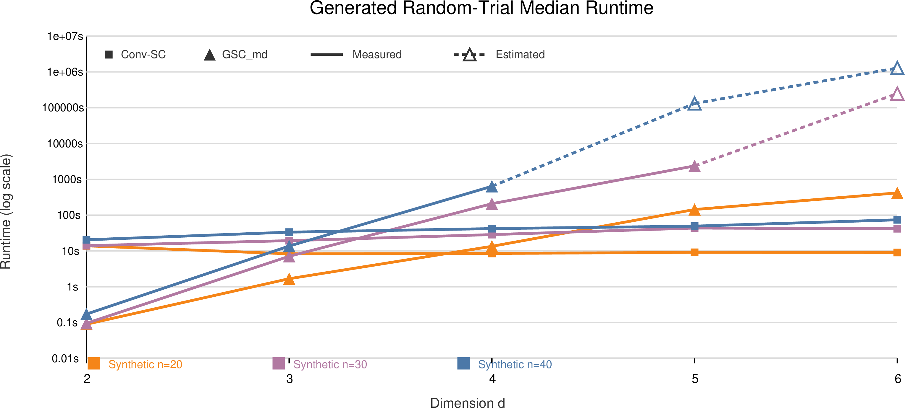
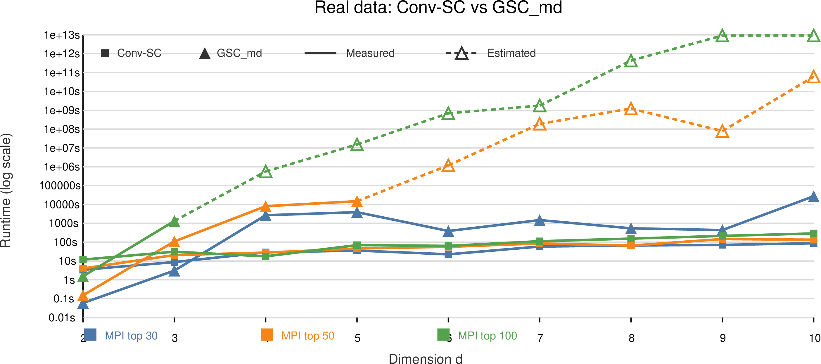
Figure 9 gives the clearest scaling evidence because generated inputs create a controlled, less correlated stress test for exact-stability computation. In this setting, Conv-SC grows smoothly with dimension, while \(GSC_{md}\) quickly moves into the high-runtime regime. Figure 10 shows the corresponding real-data behavior on MPI. The MPI indicators are correlated, so the real-data curves are less uniform than the generated curves. Even in this more structured setting, Conv-SC remains feasible through all ten indicators, while \(GSC_{md}\) increasingly depends on the runtime estimates justified above as the ranked set grows from top 30 to top 100.
8 Related Works↩︎
Our work can be viewed as an extension of [1], which investigates the stability of rankings defined by various acceptable scoring methods. More recently, [19] proposed a complementary notion of local stability for rankings. Their work studies how perturbing the data values of a single tuple can change that tuple’s position, and uses dense regions to tolerate swaps among items with similar quality. In contrast, our work keeps the dataset fixed and studies uncertainty in the scoring weights; general stability remains a global ranking-region measure, but uses ranking distances so that similar rankings can contribute differently from completely different rankings.
Our setting is also related to multi-criteria decision making and multi-criteria decision analysis (MCDM/MCDA), where alternatives are evaluated using multiple criteria and criteria weights support choices, recommendations, or rankings [20]–[22]. Robustness methods such as stochastic multicriteria acceptability analysis (SMAA) explore the weight space under uncertain or incomplete preference information [23]–[25]. These methods are typically decision- or alternative-centered: for example, SMAA reports rank acceptability indices measuring how often an alternative attains a given rank. In contrast, our object is a reported ranking as a whole. General stability evaluates the full ranking region and compares complete induced rankings through a user-defined ranking distance, distinguishing minor changes from changes that alter the substantive conclusion.
Ranking is also central in data mining. Ranking items with multiple attributes for downstream applications has motivated work on ranking [26]–[28], top-k [29], [30], and skyline queries [31]–[34].
Some work on ranking and top-k focuses on uncertainty, missing values, and noise in the dataset [35]–[37]. In contrast, ranking stability focuses on uncertainty in the scoring functions related to user preferences.
Some recent studies also apply fairness and diversity constraints to rankings [38]–[42]. For example, given a ranking weight vector, [38] seeks a similar vector with fairer results. These investigations align with our goal of supporting more responsible rankings.
As the motivation for stability originated from detecting cherry-picked models, data perturbations have also been used to identify cherry-picked trendlines [43], [44] and generalizations [45].
Our Conv-SC algorithm draws motivation from advances in computing convex-body volumes and from the hit-and-run method. Convex-body volume computation is an important problem in computational geometry; state-of-the-art works include [6], [46]. Hit-and-run sampling is also widely studied, with applications in volume computation and other domains [2], [47]–[49]; [50], [51] provided key theoretical insights on its efficiency. For geometric concepts such as half-space, see [52].
9 Conclusion↩︎
We introduced general stability, a distance-based extension of exact ranking stability that gives partial credit to rankings close to the target while recovering exact stability as a special case. We developed exact two-dimensional and sampling-based multidimensional algorithms, analyzed why fixed-error sampling can become expensive in rare-event regimes, and identified quasiconvex distance functions as a structured class where Conv-SC reduces stability computation to convex-volume approximation. Experiments on real and generated data show that distance-sensitive stability can avoid overreacting to minor ranking changes, while Conv-SC exploits convex structure to make stability computation feasible for quasiconvex distances in high dimensions. Overall, general stability offers a flexible framework for evaluating the robustness of reported rankings while letting users specify which ranking changes matter in their application.