OPINE-World: Programmatic World Modeling with
Ontology-error-Prioritized Interactive Exploration
July 01, 2026
Abstract
Learning how an environment behaves from interaction is central to building agents that adapt to unfamiliar tasks. World models learned with deep networks are flexible but data-hungry and transfer poorly beyond their training distribution. Program-synthesized world models, written as source code by LLMs and refined through counterexample-guided inductive synthesis (CEGIS), are instead data-efficient and reusable, yet they have been demonstrated mainly on structured-state worlds with a given object vocabulary, and a single program search does not scale to pixel-rendered environments whose object structure must be hypothesized flexibly. We introduce OPINE-World, an LLM agent that learns an object-centric programmatic world model online from interaction. OPINE-World couples two cooperating agents in a loop of hypothesis and test, one acting in the environment and one synthesizing the model in code with replay verification and model-based planning, and it steers exploration with a Bayesian measure of object-type adequacy we call ontology error. We evaluate OPINE-World on ARC-AGI-3, a benchmark for skill-acquisition efficiency in which the object vocabulary, the goal, and the action semantics are withheld. OPINE-World solves 20 of 25 games without per-game training and reaches an action-efficiency score of 78.4 against the human baseline.
1 Introduction↩︎
A world model predicts how an environment changes under each action, and an agent that holds one can plan and transfer to tasks that share a mechanism [1], [2]. In model-based reinforcement learning, world models learned with deep networks are general but data-hungry, and they transfer poorly beyond their training distribution [3]–[6]. A world model written as a program is the data-efficient alternative, synthesized from logged transitions and refined by counterexample-guided inductive synthesis (CEGIS), and it is inspectable and reusable [7]–[9]. Such a program is most economical when it is factored by object type, with one transition rule shared across all objects of a type, so that few parameters support many predictions and a rule learned from one object transfers to the rest [10]–[12].
Factoring helps only when the object partition is approximately correct, and in an open environment that partition is not given and must be inferred from the same interaction the rules are learned from [13], [14]. Two lines of work mark the extremes of when to commit to it. Program-synthesis-and-plan systems fix the partition at once and plan through the synthesized model, repairing it when no plan reaches reward [7], [8], [15], so a partition fixed before the data identify it carries its error into every rule built on it. Model-free agentic systems fix no structure and act from a natural-language interaction log with no synthesized model [16]–[18], keeping no reusable model and no record of what has been identified. The program-synthesis line has been shown on structured-state inputs with a given object vocabulary, and a single program search does not scale to pixel-rendered environments whose object structure must be recovered from observation [7], [8], [19].
We introduce OPINE-World, an LLM agent that learns an object-centric programmatic world model online from interaction. OPINE-World combines four mechanisms. The model is factored by object type, so a rule is repaired one type at a time. Two cooperating LLM agents run a hypothesis-and-test loop over one replay buffer. The action agent proposes hypotheses about the dynamics and the goal and probes them in the environment, guided by a natural-language world model it maintains, while the synthesizer turns each hypothesis into code and a critic challenges the fitted model for weak generalization. A candidate program is admitted only when it reproduces every recorded transition exactly. A planner then searches the verified model and validates each step against the environment. A Bayesian measure of object-type adequacy, the ontology error, steers exploration toward objects whose behavior the current types do not yet explain.
On ARC-AGI-3 [20], a benchmark for skill-acquisition efficiency in which the object vocabulary, the goal, and the action semantics are withheld, OPINE-World solves 20 of 25 games without per-game training, surpasses a strong single-agent coding baseline, and stays under the human action count on most of the games it solves, while program-synthesis and neural latent world models solve none.
1.0.0.1 Contributions.
OPINE-World, an LLM agent that learns object-centric programmatic world models online from interaction, running a hypothesis-and-test loop of two cooperating LLM agents with counterexample-guided synthesis and model-based planning (Section 3).
A method that discovers the object ontology from interaction, where prior program-synthesized world models receive a structured state with a given object vocabulary, which extends them to pixel-rendered environments with unknown object structure (Section 3).
An evaluation on ARC-AGI-3 in which OPINE-World solves 20 of 25 games and 160 of 183 levels without per-game training, exceeding a strong single-agent coding agent, while program-synthesis and neural latent world models solve none (Section 4).
2 Problem Setting↩︎
2.0.0.1 Object-oriented MDP.
We model an interactive environment as an object-oriented Markov decision process [10] and instantiate it on ARC-AGI-3. A game is a tuple \((\mathcal{C},\mathcal{A},T,R,s_0)\) with object classes \(\mathcal{C}\), a finite action set \(\mathcal{A}\), a deterministic transition \(T:\mathcal{S}\times\mathcal{A}\to\mathcal{S}\), a reward \(R\), and a level-entry state \(s_0\). A structured state \(s\in\mathcal{S}\) is a finite collection of typed objects \(o=(\text{name},\tau,\mathbf{v})\), where \(\tau\) is a type and \(\mathbf{v}\) holds atomic attributes such as position, visibility, rotation, and a small pixel pattern. The action set contains directional moves, a select action, and a pointer click. The meaning of each action is not given, and the agent recovers it by acting.
2.0.0.2 Perception and what is withheld.
The engine exposes each frame as a raw \(64\times64\) grid of color indices, with no sprite list, object identities, or types. OPINE-World synthesizes its own perception, an extractor \(\alpha\) that segments a frame into object records carrying a position, a visibility flag, and a small pixel pattern, and pairs them across time. What is withheld is the rest. The partition of the objects into mechanical types is unknown, the goal is unstated, the actions are anonymous, and no demonstration is provided. The agent infers the type partition from observation, reads goal relevance from the reward it observes, and discovers action effects by trying actions in context.
2.0.0.3 Reward and scoring.
Reward is sparse. The environment reports success on a level advance and is otherwise silent. A game is a sequence of levels, and clearing the last level wins the game. An agent is scored on the number of actions it spends, so an agent that re-derives a mechanic it has already seen pays for the repetition. We report the action count to clear a game and whether all levels were cleared.
2.0.0.4 World model and verification.
A world model is a Python transition \(\widehat T\) written by a language model and repaired by counterexample-guided synthesis against the replay buffer \(\mathcal{D}_t=\{(s_i,a_i,s_i')\}_{i\le t}\). The acceptance test is exact replay, \[\phi(\mathcal{D}_t,\widehat T):\quad \widehat T(s_i,a_i)=s_i'\;\text{ for all }\;(s_i,a_i,s_i')\in\mathcal{D}_t .\] We do not synthesize a reward function in the optimism sense of earlier work [7], [21]. Goal recognition uses the observed reward before a level is cleared, and a synthesized Boolean goal predicate after, checked by the same exact-replay test [7], [15].
Assumption 1 (Observable-Markov determinism). There is a representation of the structured state under which \(T\) is a deterministic function of the state and action. Conditioned on a correct partition into types and a sufficient local context, the effect of an action on each object is a single outcome.
Assumption 1 is what makes the exact-replay test well posed. Where it fails, for example under hidden state, the test still rejects wrong models, and the ontology error of Section 3 has a floor it cannot drive to zero. We return to that case in Section 6.
3 Method↩︎
OPINE-World runs one loop over a growing record of interaction (Figure 1). The goal-directed agent takes an action in the live game and appends the resulting transition to a shared buffer. The world-model agent reads the buffer and, when the current model has been contradicted, rewrites the object-centric program so that it again reproduces every recorded transition. Once a model has been admitted and at least one level has been cleared, a planner searches the model for a route to the goal, and the route is executed one step at a time against the live game. A Bayesian measure of how well the current object types explain the recorded effects runs alongside the loop and steers where the agents look next. The rest of this section describes these four mechanisms.
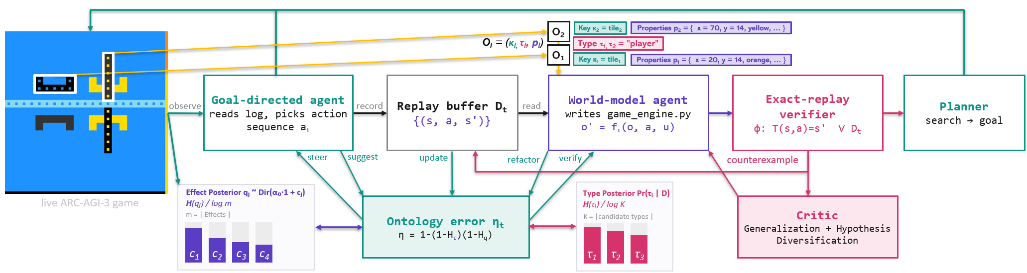
3.1 An object-centric world model↩︎
3.1.0.1 A factored program.
A structured state is a finite set of typed objects, \[s_t=\{o_t^i\}_{i\in I_t}, \qquad o_t^i=(\kappa_t^i,\tau_t^i,\mathbf{v}_t^i),\] where \(\kappa\) is a matching key, \(\tau\) a mechanical type, and \(\mathbf{v}\) an attribute map over position, visibility, rotation, and a small pixel pattern. The world model is a program organized by type: for each type \(\tau\) it holds a response rule \[f_\tau:\mathcal{O}_\tau\times\mathcal{A}\times\mathcal{X}\to\mathcal{O}_\tau,\] a function from an object of type \(\tau\), an action, and a read-only local context \(\mathcal{X}\) over the pre-action state, to the updated object. Pairing each before-object \(i\) with an after-object \(\mu_t(i)\), the rule predicts \[o_{t+1}^{\mu_t(i)} \approx f_{\tau_t^i}\!\left(o_t^i,\,a_t,\,u_t^i\right), \qquad u_t^i=\psi(o_t^i,s_t),\] where \(u_t^i\) is a local context feature and the transition \(\widehat T\) applies the matching \(f_\tau\) to every object and collects the results. A program that places all behavior in one type degenerates to a single monolithic transition. The factored form subsumes STRIPS operators, where the add and delete lists are the difference between an object before and after, with conditional effects organized by type rather than enumerated [22]–[24].
3.1.0.2 Why structure stays local.
Organizing the program by type ties many predictions to few rules, and it lets a rule learned from one object apply to every object of its type [10], [12], [25]. The benefit holds only when the grouping is close to correct. A group that joins objects with different dynamics ties one rule across mismatched data, and the rule is biased wherever the objects differ. OPINE-World does not force one object per type and does not commit a partition in advance. Objects in ARC-AGI-3 are often fragments of a single behavioral unit, such as a bridge drawn from several sprite ids or a counter built from separate glyphs, and forcing such fragments into separate types splits one rule across type boundaries. Because each rule is attached to a type and is repaired one type at a time, a wrong grouping is corrected locally and does not spread through the rest of the model.
3.2 Two cooperating agents↩︎
3.2.0.1 Acting and modeling are separate jobs.
Decoupling the agent that gathers experience from the one that fits the model is a long-standing design in reinforcement learning [1], [26], [27], and cooperating language-model agents with specialized roles have outperformed a single agent on multi-step tasks [28]–[30]. OPINE-World runs two language-model agents over the shared buffer. The goal-directed agent plays the live game. It reads the interaction log with ordinary file tools, runs short scripts over it, and chooses the next action or short sequence of actions. The world-model agent writes and repairs the program. It reads the same buffer and the diagnostics, proposes a program, and submits it to the verifier. The two never write to each other’s artifacts, and they communicate only through the buffer and a short structured handoff.
3.2.0.2 Proposal comes from the language model, guarantees from the verifier.
The language model supplies what a discrete search cannot. It proposes a partition of the scene into types, names candidate roles for objects, and writes code that generalizes a handful of transitions into a rule [31], [32]. These proposals are cheap to generate and expensive to verify by enumeration, which is the regime where a language model is most useful [33], [34].
3.2.0.3 A loop of hypothesis and test.
The two agents, together with a periodic critic, run a loop of hypothesis and test [34]–[36]. The action agent proposes hypotheses about the dynamics and the goal, drawn from a natural-language world model that the agents keep in shared notes and from the current synthesized model, and it explores to probe them. The synthesizer turns a hypothesis into code, and the exact-replay check accepts or refutes it. A critic runs on a fixed cadence and challenges a fitted model for weak generalization, asking which parts are tailored to one level and would fail on a new layout, which presses the synthesizer to weigh competing hypotheses rather than commit to the first that fits.
3.3 Verification and counterexample-guided synthesis↩︎
3.3.0.1 Acceptance is an exact check.
A proposed program is admitted only when it reproduces every transition in the buffer exactly, \[\phi_T(\widehat T,\mathcal{D}_t):\quad \widehat T(s_\ell,a_\ell)=s_{\ell+1} \;\text{ for all }\;(s_\ell,a_\ell,s_{\ell+1})\in\mathcal{D}_t,\] attribute for attribute and object for object. Acceptance is a decision rather than a score [37], [38]. A program is also run twice on each transition, and a program whose two runs differ is rejected, which removes any model that depends on hidden state and would break a forward planner. The goal predicate is checked the same way once reward has been observed, and a static check rejects a predicate that recognizes the goal by reading a cached future state rather than by testing the goal mechanic.
3.3.0.2 Repair follows counterexamples.
Synthesis does not run on a schedule. The world-model agent builds the first model once enough transitions exist, and after that it rewrites only when the live model mispredicts an observed transition. A mispredicted transition is a counterexample [9], [39], and it serves both as a constraint for the next program and as a real observation that updates the diagnostics. A short deferral window lets a few counterexamples accumulate before a rewrite, and a stall guard stops repeated rewrites that fail to improve accuracy until a fresh counterexample arrives.
3.4 Object-type diagnostics and ontology error↩︎
Alongside the program, OPINE-World keeps a cheap Bayesian diagnostic that scores how well the current types explain what it has seen and steers exploration toward what they do not. It is built from coarse effect signatures rather than exact deltas.
3.4.0.1 Effect signatures.
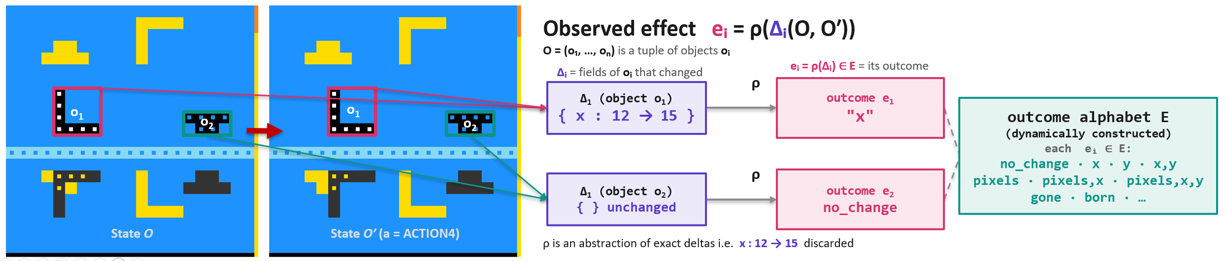
For a paired object let \(\Delta_t^i\subseteq\mathsf{Attr}(\tau_t^i)\) be the attributes that changed; a quotient map \(\rho\) sends it to a categorical signature from an alphabet \(\mathcal{E}\) grown from what is observed, \[\Delta_t^i=\{\,b:\mathbf{v}_{t+1}^{\mu_t(i)}(b)\neq\mathbf{v}_t^i(b)\,\}, \qquad e_t^i=\rho(\Delta_t^i)\in\mathcal{E},\] recording which attributes changed and discarding the values (Figure 2).
3.4.0.2 The local effect table.
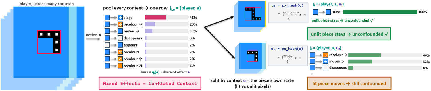
Each object-transition is filed into a row keyed by type, action, and local context, \(j=(\tau,a,u)\), and the table counts signatures per row, \(C_t(j,e)\). A symmetric Dirichlet prior yields a posterior over the row’s effect distribution and its mean, \[q_j\mid\mathcal{D}_t\sim\mathop{\mathrm{Dir}}(\alpha_0\mathbf{1}_m+\mathbf{c}_j), \qquad \widehat q_j(e)=\frac{\alpha_0+C_t(j,e)}{m\alpha_0+\sum_{e'}C_t(j,e')}.\] A row that mixes signatures is under-observed or missing a context feature, and adding a before-state feature \(u\) can split it into concentrated subrows (Figure 3).
3.4.0.3 Ontology error.
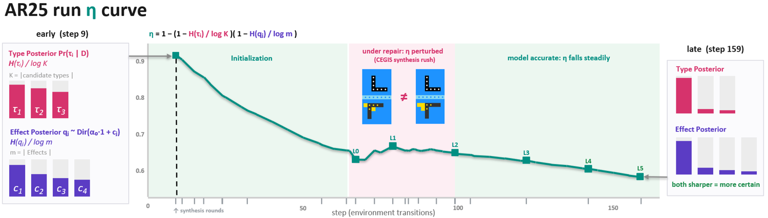
Two normalized entropies measure what is unresolved, the type uncertainty of an object and the effect uncertainty of its row, \[U_i^{\rm type}=\frac{\mathsf H[\Pr(\tau_t^i\mid\mathcal{D}_t)]}{\log K}, \qquad U_{j}^{\rm row}=\frac{\mathsf H(\widehat q_{j})}{\log m}\;\in[0,1],\] and their noisy-OR is the per-object ontology error, averaged into the aggregate \[\eta_t^i=1-(1-U_i^{\rm type})(1-U_{j_t^i}^{\rm row}), \qquad \eta_t=\frac{1}{N_t}\sum_{\ell<t}\sum_{i\in I_\ell}\eta_\ell^i .\] A high \(\eta_t^i\) marks objects and contexts the current types do not yet explain, so the goal-directed agent probes them and the synthesizer refines a type or adds a context feature, in line with exploring to reduce model uncertainty [40]–[42]. A falling \(\eta_t\) tracks the ontology settling over a run (Figure 4), while correctness is decided not by \(\eta\) but by the exact-replay test below. Appendix 13 gives the full construction.
3.5 Planning over the verified model↩︎
Once a model has been admitted and a level has been cleared, the world-model agent writes a planner over the verified model \(\widehat M=(\mathcal{S},\mathcal{A},\widehat T,\widehat G)\), a bounded forward search for an action sequence that reaches a goal state under \(\widehat T\) and the goal predicate \(\widehat G\). The planner is first checked offline by planning to reward from the entry states of the levels already cleared. A plan that passes is executed against the live game one step at a time. Each executed step is compared with the model’s prediction. A match continues the plan, and a mismatch ends it, records the offending transition as a counterexample, and returns control to the goal-directed agent. A plan that reaches the goal confirms the win at its action count.
4 Experiments↩︎
4.0.0.1 Setup.
We evaluate OPINE-World on ARC-AGI-3 [20], a benchmark for skill-acquisition efficiency, using its public evaluation set of 25 games. Each game is a sequence of levels with a sparse level-advance reward, and an agent is scored on the actions it spends and on how many levels it clears. OPINE-World plays each game online under the live, on-policy budget, with no reset to re-sample a level. We report the action count to clear a game, the levels cleared, and the outcome. The synthesis and action agents run Claude Opus 4.8 behind a filesystem sandbox, described in Appendix 8. Neither OPINE-World nor baseline1 is trained, fine-tuned, or shown demonstrations on the evaluation games. The language model is a general pretrained model that is not updated, and the agent learns each game’s mechanics online during the scored run, from raw rendered frames.
4.0.0.2 Baselines.
The strongest comparison without per-game training is a single-agent object-centric coding agent, called baseline1 here, which synthesizes an executable world model, verifies it against past transitions, and plans through it, all within one agent driven by a strong reasoning model. As publicly reported, baseline1 runs GPT-5.5 at high reasoning effort, and OPINE-World runs Claude Opus 4.8, so the comparison is between systems that use different base models rather than a single controlled variable, and a same-model study is left to future work. We report two reference points that fail outright. WorldCoder searches for one program that explains the whole game and repairs it under an optimism constraint [7], and a set of neural latent world models in the Dreamer and MuZero families learn dynamics in a latent space [3]–[5]. We list separately a continual-learning vision agent, called Vision here, which explores the public game set offline and accumulates weights, then plays the scored run with those weights frozen. Because Vision trains on the very games it is later scored on, its action counts measure performance after exposure to the evaluation games. We mark it accordingly and keep it out of the no-training comparison.
| System | Score (%) | Games won | Mean levels | Note |
| (/25) | cleared | |||
| OPINE-World (ours) | 78.4 | 20 | 0.90 | no per-game training |
| baseline1 | 63.8 | 14 | 0.80 | single-agent coding agent |
| Vision | 63.2 | 12 | 0.73 | pre-trains on eval set |
| WorldCoder | 0.0 | 0 | 0.00 | clears no level |
| Latent world models | 0.0 | 0 | 0.00 | clears no level |
4.0.0.3 OPINE-World leads on the benchmark’s action-efficiency score.
ARC-AGI-3 scores an agent by how few actions it spends against a human baseline. Each level scores \((\text{human}/\text{agent})^2\) capped at \(1.15\), levels are weighted by their index, and the per-game score is capped at \(100\), so a game reaches \(100\) only when every level is cleared at or above human pace. Figure 5 reports the per-game scores. OPINE-World reaches a total of \(78.4\) over all 25 games, where baseline1 reaches \(63.8\) and the pretrained Vision agent \(63.2\).

4.0.0.4 OPINE-World clears more games than the baseline.
Table 1 summarizes the set, and Table 3 reports every game. OPINE-World clears 20 of the 25 games. baseline1 clears 14. Of the 14 games baseline1 clears, OPINE-World clears 13, the lone exception being ka59, and OPINE-World additionally clears seven games that defeat baseline1 outright. WorldCoder and the neural latent world models clear no game under the benchmark’s budget. Figures 6, 7, and 8 visualize the comparison, and Appendix 11 adds coverage, a per-game scatter, and a levels-cleared heatmap.
4.0.0.5 The decisive margin is on the hard games.
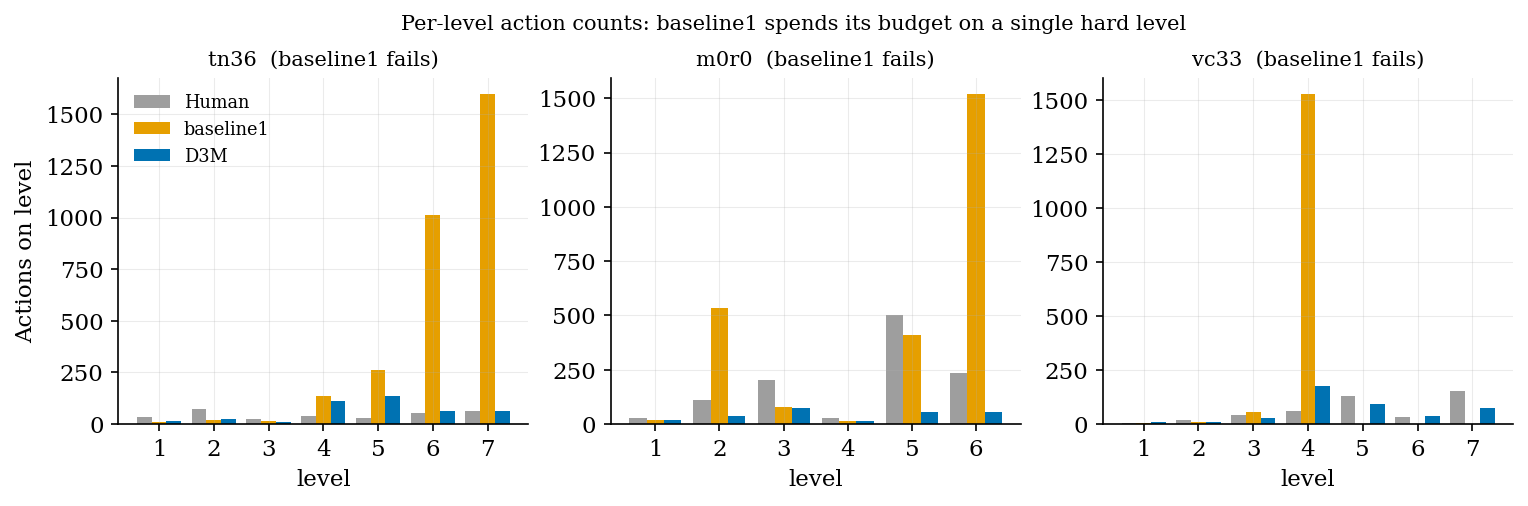
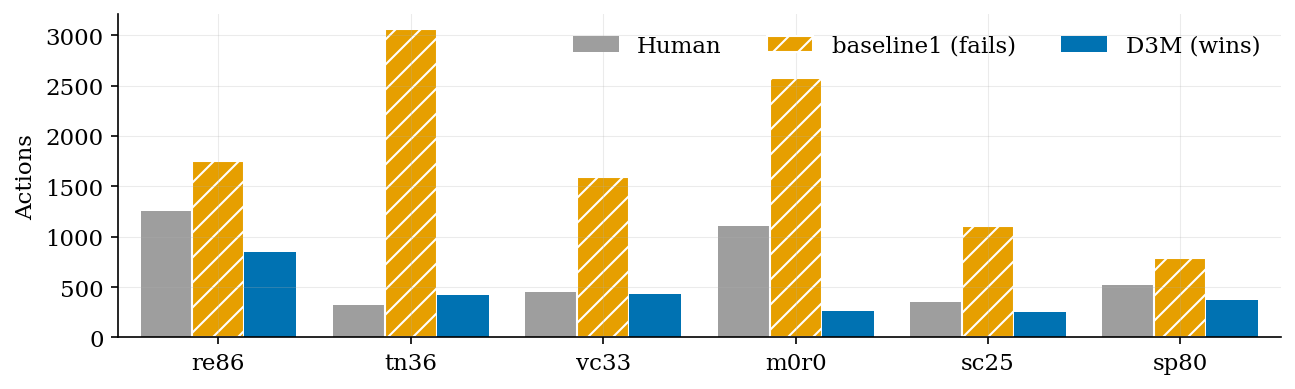
Six games defeat baseline1 entirely (Table 2). On re86, tn36, vc33, m0r0, sc25, and sp80, baseline1 exhausts its budget without clearing the game, after spending 10,874 actions in total across the six. OPINE-World clears all six, and it does so in 2,578 actions in total, about a quarter of what baseline1 spent before failing. On the same six games the human reference uses 3,994 actions, so OPINE-World clears them in about two thirds of the human budget. OPINE-World also wins dc22, a seventh game baseline1 fails, at a higher cost of 1,479 actions. Two effects produce the margin. OPINE-World clears games that defeat a strong single agent, and it avoids spending thousands of actions on a game it cannot yet model. The easy games both agents solve add little.
4.0.0.6 On games both solve, the two are comparable.
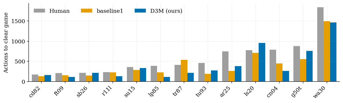
On the thirteen games that both OPINE-World and baseline1 clear, the action counts are close. OPINE-World uses fewer actions on six of them and baseline1 uses fewer on seven, and the totals are within a fraction of a percent of each other. OPINE-World’s advantage over a strong single agent lies in covering harder games and in holding back action counts when a game is hard to model.
4.0.0.7 OPINE-World is action-efficient against the human reference.
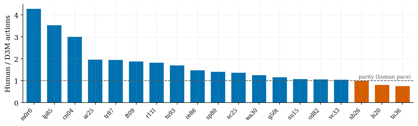
On 16 of its 20 wins, OPINE-World clears the game in fewer actions than the human reference. It uses more on four of them, by a single action on sb26 and by wider margins on ls20, tn36, and dc22. Averaged over its wins, the ratio of human actions to OPINE-World actions is 1.7, with the largest margins on m0r0 (4.3), lp85 (3.5), and cn04 (3.0).
4.0.0.8 A note on Vision.
The continual-learning vision agent reaches a higher raw scorecard on the public set, near 63%, and it clears 12 of 25 games in the scored run. Its offline phase plays the same public games and grows the weights it then freezes, so the action counts in its scored run follow earlier passes over those games. We include it for completeness and do not treat it as a no-training result. OPINE-World clears more games than Vision, 20 against 12, even though Vision trains on the evaluation games beforehand.
4.0.0.9 Ablations.
We compare against a strong single agent and against failing reference points. Due to the heavy interdependency of each sub-component, where a naive removal of any component in isolation will cause system instability, we leave more targeted per-component ablations to future work.
| Game | Human | baseline1 | OPINE-World | |
|---|---|---|---|---|
| 3-4(lr)5-5 | Act. | Act. | Levels | Act. |
| re86 | 1255 | 1754 | 4/8 GO | 850 |
| tn36 | 317 | 3058 | 6/7 GO | 417 |
| vc33 | 447 | 1596 | 3/7 GO | 427 |
| m0r0 | 1107 | 2573 | 5/6 GO | 259 |
| sc25 | 350 | 1107 | 3/6 GO | 256 |
| sp80 | 518 | 786 | 1/6 GO | 369 |
| Total | 3994 | 10874 | 2578 | |
6pt
| baseline1 | OPINE-World (ours) | Vision | ||||||||
|---|---|---|---|---|---|---|---|---|---|---|
| 3-5(lr)6-8(lr)9-11 Game | Human | Act. | Lvl | Res | Act. | Lvl | Res | Act. | Lvl | Res |
| tu93 | 462 | 192 | 9/9 | WIN | 9/9 | 50 | 0/9 | GO | ||
| sb26 | 213 | 150 | 8/8 | WIN | 214 | 8/8 | WIN | 143 | 8/8 | WIN |
| lp85 | 388 | 226 | 8/8 | WIN | 8/8 | 391 | 7/8 | GO | ||
| ar25 | 748 | 264 | 8/8 | WIN | 381 | 8/8 | WIN | 262 | 8/8 | WIN |
| tr87 | 414 | 540 | 6/6 | WIN | 6/6 | 268 | 6/6 | WIN | ||
| r11l | 233 | 227 | 6/6 | WIN | 6/6 | 40 | 2/6 | GO | ||
| ft09 | 208 | 157 | 6/6 | WIN | 6/6 | 128 | 6/6 | WIN | ||
| cd82 | 171 | 130 | 6/6 | WIN | 161 | 6/6 | WIN | 153 | 6/6 | WIN |
| cn04 | 789 | 448 | 6/6 | WIN | 6/6 | 289 | 6/6 | WIN | ||
| su15 | 361 | 284 | 9/9 | WIN | 334 | 9/9 | WIN | 89 | 3/9 | GO |
| re86 | 1255 | 1754 | 4/8 | GO | 8/8 | 722 | 8/8 | WIN | ||
| tn36 | 317 | 3058 | 6/7 | GO | 7/7 | 95 | 5/7 | GO | ||
| vc33 | 447 | 1596 | 3/7 | GO | 7/7 | 94 | 2/7 | GO | ||
| m0r0 | 1107 | 2573 | 5/6 | GO | 6/6 | 41 | 0/6 | GO | ||
| sc25 | 350 | 1107 | 3/6 | GO | 6/6 | 165 | 6/6 | WIN | ||
| sp80 | 518 | 786 | 1/6 | GO | 6/6 | 195 | 5/6 | GO | ||
| wa30 | 1843 | 1495 | 9/9 | WIN | 9/9 | 648 | 9/9 | WIN | ||
| g50t | 879 | 554 | 7/7 | WIN | 757 | 7/7 | WIN | 526 | 4/7 | GO |
| ls20 | 776 | 714 | 7/7 | WIN | 959 | 7/7 | WIN | 462 | 7/7 | WIN |
| ka59 | 730 | 1099 | 7/7 | WIN | 1076 | 6+/7 | GO | 312 | 7/7 | WIN |
| dc22 | 1228 | 1842 | 4/6 | GO | 6/6 | 550 | 4/6 | GO | ||
| sk48 | 1070 | 2823 | 5/8 | GO | 596 | 4+/8 | GO | 339 | 4/8 | GO |
| lf52 | 1339 | 2646 | 6/10 | GO | 593 | 3+/10 | GO | 919 | 10/10 | WIN |
| bp35 | 651 | 342 | 4/9 | GO | 512 | 2+/9 | GO | 204 | 6/9 | GO |
| s5i5 | 638 | 3028 | 3/8 | GO | 638 | 4+/8 | GO | 331 | 4/8 | GO |
| Won | 14/25 | 20/25 | 12/25 | |||||||
5 Related Work↩︎
5.0.0.1 Program-synthesized world models.
WorldCoder and PoE-World synthesize an executable world model, plan through it, and summarize what is known about the world as a binary distinction between learned and unlearned [7], [8]. TheoryCoder adds a hand-designed layer of PDDL predicates and operators above the synthesized dynamics and plans at two levels [15]. OPINE-World keeps the synthesized executable model and the counterexample loop, and it differs in four ways. It separates acting from modeling across two agents, it discovers the object and role layer from data rather than receiving it by hand, it admits a model only by exact replay rather than by an optimism or likelihood criterion, and it gates the planner on having cleared a level and validates each planned step against the live game. It also drops the synthesized reward function and the optimism constraint that the earlier systems carry.
5.0.0.2 Model-free agentic exploration.
A coding agent can play these games by reading a log of its own interaction and selecting the next action, with no synthesized dynamics [16]. The approach never commits to a wrong model, and it keeps no reusable model, no way to simulate a counterfactual, and no record of what has been pinned down. OPINE-World adopts the read-and-script pattern for its goal-directed agent and restores the verified model and the diagnostic that a log-only agent forgoes.
5.0.0.3 Neural and latent world models.
Latent-dynamics models learn to predict and plan in a learned state space and have mastered arcade and control domains with large amounts of interaction [3]–[5]. Sample efficiency improves with explicit model learning [1], [6], and the data these models need is still far beyond the action budget of a single ARC-AGI-3 game, while a learned latent state space transfers poorly to a new game with a new ontology, where object-centric models with per-entity rules generalize across layouts [43], [44]. OPINE-World uses a program with shared per-type rules, so a handful of transitions identifies a rule and that rule transfers to every object of its type.
5.0.0.4 Bayesian structure and language-model proposals.
The object and role layer that OPINE-World infers is a partition-learning problem, and the Dirichlet effect counts and role posterior follow Bayesian structure learning and relational clustering [13], [14], [45]. A growing line uses a language model to propose programs or theories that are then scored against data [35], [46]–[48]. These systems usually receive at least one structural prior that ARC-AGI-3 withholds, such as a fixed ontology, named actions, or a stated goal, and they score proposals by likelihood. OPINE-World composes the language-model proposal with an exact replay test that the observable-Markov assumption makes well posed. For planning over the learned model, OPINE-World uses bounded forward search in the style of width-based planners over simulators [49], [50], and it follows the practice of writing a planner once rather than scoring each search node with a model call [51], [52]. The generate-test-repair loop is Reflexion-style iteration [53]–[55], and the symbolic analogue of learning an action model inside a planning loop is classical action-model learning [56]–[58].
6 Limitations↩︎
Observable-Markov scope. The exact-replay test and the epistemic measure assume that the state and action determine the next state under some representation (Assumption 1). Under hidden state the test still rejects wrong models, and the measure has a floor it cannot drive to zero, so the timing signal degrades. Hidden-state games are out of scope here.
Inferred perception. OPINE-World works from raw frames and synthesizes its own object extractor, so pairing and the type partition are inferred rather than given. Engine-given object identities would make the pairing \(\mu_t\) exact and the initial type assignment informative, driving \(U_i^{\rm type}\to0\) so the ontology error \(\eta_t^i\) collapses to the row uncertainty \(U_{j_t^i}^{\rm row}\) alone, a sharper signal we leave to future work.
Planner scale. The synthesized planner is a bounded forward search, and on games with a high branching factor a naive search reaches its bound without a plan, which returns control to the goal-directed agent. A stronger synthesized search would extend the reach of the planning phase.
Single run per game. Each game is played once, so the table carries no variance estimate, and the headline counts could shift by a few games under resampling.
7 Conclusion↩︎
OPINE-World learns an object-centric programmatic world model online from interaction by running a hypothesis-and-test loop. Two cooperating LLM agents propose and verify the model, counterexample-guided synthesis keeps it consistent with every observed transition, and a planner searches the verified model to reach the goal. On the ARC-AGI-3 public set OPINE-World solves 20 of 25 games and 160 of 183 levels without per-game training and exceeds a strong single-agent coding agent on the benchmark’s action-efficiency score, where program-synthesis and neural latent world models solve none. Extending the approach to stochastic and partially observed environments, and to raw-pixel perception, is left to future work.
The appendix records how the loop of Section 3 is realized (Appendix 8), the design choices behind it (Appendix 9), the integrity checks on the evaluation (Appendix 10), and the full formal construction of the model and its ontology error, additional result visualizations (Appendix 11), and the full formal construction (Appendix 13 onward).
8 Implementation and System Details↩︎
The components of Section 3 are realized in the running system as follows. OPINE-World runs two language-model agents over one shared replay buffer of observed transitions, together with a planner that the second agent writes as code. The goal-directed action agent plays the live game. The world-model synthesis agent writes and repairs the executable model. The planner searches that model after the model has been admitted and a level has been cleared.
8.1 The world model artifact↩︎
The synthesis agent maintains a single Python file, game_engine.py. The file exposes transition_function(state, action), which returns the predicted next state, and reward_function(state), which returns the
predicted reward and a goal flag for a state. The file may also export a planner() hook and, in frames mode, an extract_objects(frame) function that recovers an object representation from a raw \(64\times64\) frame. The synthesis agent is free to choose any internal organization that fits the observations, including plain functions, classes, or lookup tables. The form is selected by the agent rather than fixed by the
harness.
8.2 Per-role responsibilities↩︎
The action agent reaches reward in the live environment using read-only tools over a monotonic interaction log and a Python interpreter. The agent reads and greps the log and runs short scripts over it, and the agent never edits the model. The synthesis
agent runs in the background and refines transition_function, and after a level has been cleared it also refines reward_function. The planner runs a bounded forward search over the current transition_function and
reward_function, or over the synthesizer’s own planner() hook when one is present. Roles are separated by objective alone. No orchestrator subagent sits above them.
8.3 Verification↩︎
A candidate model is admitted only after it passes the replay check. Every transition in the buffer is replayed through transition_function, and the predicted next state is compared for exact equality against the observed next state. The
predicted reward and goal flag are compared against the observed reward in the same pass. A single mismatch rejects the candidate. Each transition is also evaluated twice, and a candidate whose two outputs differ is rejected, which removes any model that
carries hidden module-level state, because the forward planner assumes a pure deterministic transition. The verifier also applies a static check to the body of reward_function. A predicate that recognizes the goal by reading the cached entry
state of a later level is rejected by that check, because such a predicate passes the replay check trivially while encoding nothing about the goal mechanic.
8.4 Synthesis cadence↩︎
Synthesis is triggered by counterexamples rather than run on a fixed schedule. The synthesis agent fires once to build the first model. After that, it fires only when the live model mispredicts an observed transition. A short deferral window lets a few moves and errors accumulate before the agent re-fires, so a single surprising step does not restart synthesis on its own. A stall guard stops the agent from re-firing after two rounds that fail to improve transition accuracy, and the agent waits for a fresh counterexample before trying again.
8.5 Multi-tick actions↩︎
A single action can animate over several internal engine ticks before the state settles, as happens with water flow, gravity, or a chain reaction. The model predicts the settled after-state, and the replay check compares against that settled state. The intermediate per-tick frames are surfaced to the synthesis agent as extra evidence, because a mechanic that plays out and reverts before settling leaves no signature in the before-and-after pair on its own.
8.6 Context discipline↩︎
Each agent runs under a uniform compaction discipline. On crossing a per-game token threshold, the active agent emits a structured handoff and its session is reset. The successor agent reads the handoff and resumes from it. Compaction is local to each role and is otherwise transparent to the formalism.
8.7 Sandboxing and resume↩︎
The synthesis agent and both playing agents run filesystem-confined under bubblewrap or under Docker with a filtered network, so the ground-truth game source cannot be read. The dynamics are inferred from observation. Runs are snapshotted, and a run resumes deterministically by resetting the environment and replaying the recorded action sequence, which reconstructs the exact environment state.
9 Design Rationale↩︎
The forms used in Section 3 are the outcome of a design loop that discarded several plausible alternatives. We record the load-bearing choices here so that a reader who asks why an obvious option was avoided has a referent.
9.1 No synthesized reward function in the WorldCoder sense↩︎
Earlier programmatic world-model systems synthesize a reward function alongside the transition function and drive a planner with it [7], [8]. We carried this structure in early drafts and found that nothing in the system depends on a synthesized reward over hypothetical futures. Action selection runs
in the live environment on the environment’s own reward signal. Goal relevance is read from reward observed on the trajectory. A later system in the same line encodes goals as predicates over observed state rather than as a synthesized reward function
[15], and we reached the same conclusion. Dropping the synthesized reward removes the optimism constraint that WorldCoder imposes,
and it matches what the ARC-AGI-3 environment provides at observation time. The synthesized reward_function that the system does maintain is a goal predicate over the structured state, fitted only after reward has been observed.
9.2 Forward search rather than regression↩︎
Regression planning presupposes a goal written as a conjunction of facts with operators that declare which facts they add and delete, the STRIPS form [22]. The synthesized goal predicate is a Boolean function over the structured state with no such factored representation. Backward chaining over it would require a second synthesis layer to recover an add-and-delete schema, which doubles the synthesis surface and adds a failure mode in which a wrong schema yields a wrong regression. TheoryCoder pays this cost by hand-writing the schema in PDDL [15]. We avoid the second layer. Forward search is well posed directly over the artifact, and forward search over learned models is the dominant choice in this literature, from MuZero [4] to width-based arcade planners [50].
9.3 Counterexample-triggered synthesis rather than a fixed cadence↩︎
Re-synthesizing on a fixed schedule spends model calls when the current model already predicts every observed transition. Firing on counterexamples spends a call only when the live model has been contradicted by an observation, which is the only event that supplies new constraint for the verifier. The deferral window and the stall guard of Appendix 8.4 keep the loop from thrashing on a single surprising step or on a repair the agent cannot find, and they return control to the action agent for more exploration when synthesis stalls. The generate-test-reflect shape follows Reflexion-style iteration [53].
9.4 Why the planner is gated and verified↩︎
The planner is allowed to fire only after at least one level has been cleared. By the time the first level-advance reward fires, the buffer has exercised the sprite types the goal mechanic touches, so the model has the evidence a plan would rely on. Before the planner is used on the live game, it is verified offline by planning to reward from the entry states of completed levels. A plan is then executed one real step at a time, and any mismatch between a predicted step and the observed step becomes a counterexample that returns control to the action agent and reopens synthesis. The per-step check is the runtime form of a plausibility test, so a separate pre-flight probe before each invocation would catch the same failures at extra cost and is omitted. There is no engine forward-search fallback once the planner is in use. Per-node language-model scoring of search states [52] is avoided because it pays one model call per expansion, which is infeasible at the branching factor of an ARC-AGI-3 level, and the heuristic-once-per-domain posture [51] motivates keeping search at full speed.
9.5 Why the model must be inferred and not read↩︎
The agents run filesystem-confined so that the ground-truth game source is unreadable, which forces the model to be inferred from observation. A model-free agent over a monotonic log is the read-grep-shell pattern this design borrows for the action role [16], and the synthesized artifact restores the executable model and the exact replay check that such an agent forgoes. Classical action-model learning shares the planner-in-loop structure with symbolic synthesis in place of language-model synthesis [56].
10 Integrity of the Evaluation↩︎
Because the agents run language models with shell access, we checked that no run read the ground-truth game source, the web, or stored credentials. The agents are filesystem-confined so that the directories holding the environment source are never mounted to them. A full audit of the action and synthesis transcripts across four sweeps found no successful access to game source and no network use. Several explicit attempts to locate the source were present in the transcripts, and the filesystem confinement blocked all of them, returning only the run directory. The synthesized models open only their own buffered state files. One failure mode the audit surfaced is a goal predicate that recognizes a level advance by reading a cached entry state of the next level, which passes the replay test trivially. A static check on the predicate body rejects that pattern, as recorded in Appendix 8.3. The structured-state results reported here therefore reflect dynamics inferred from interaction rather than copied from the environment.
11 Additional Result Visualizations↩︎


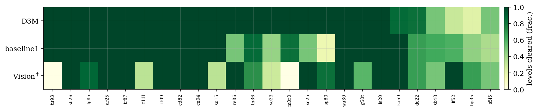
12 Per-Level Action Counts↩︎
Table 1 reports the actions each system spent on every level of every game, the per-level data behind the figures in Section 4.
| Game | System | L1 | L2 | L3 | L4 | L5 | L6 | L7 | L8 | L9 | L10 |
|---|---|---|---|---|---|---|---|---|---|---|---|
| Game | System | L1 | L2 | L3 | L4 | L5 | L6 | L7 | L8 | L9 | L10 |
| tu93 | Human | 19 | 16 | 34 | 42 | 123 | 80 | 14 | 23 | 111 | |
| baseline1 | 18 | 16 | 19 | 18 | 29 | 28 | 14 | 21 | 29 | ||
| D3M | 22 | 32 | 19 | 37 | 31 | 36 | 14 | 25 | 55 | ||
| sb26 | Human | 18 | 28 | 18 | 19 | 31 | 23 | 58 | 18 | ||
| baseline1 | 13 | 15 | 15 | 15 | 17 | 19 | 39 | 17 | |||
| D3M | 13 | 47 | 31 | 15 | 17 | 39 | 35 | 17 | |||
| lp85 | Human | 17 | 38 | 31 | 16 | 41 | 60 | 26 | 159 | ||
| baseline1 | 14 | 138 | 19 | 13 | 10 | 20 | 5 | 7 | |||
| D3M | 8 | 12 | 17 | 16 | 11 | 20 | 8 | 17 | |||
| ar25 | Human | 32 | 50 | 75 | 37 | 89 | 159 | 233 | 73 | ||
| baseline1 | 17 | 14 | 41 | 22 | 30 | 56 | 37 | 47 | |||
| D3M | 17 | 16 | 75 | 24 | 34 | 55 | 112 | 47 | |||
| tr87 | Human | 54 | 58 | 40 | 45 | 71 | 146 | ||||
| baseline1 | 47 | 190 | 47 | 36 | 47 | 173 | |||||
| D3M | 33 | 29 | 26 | 27 | 22 | 74 | |||||
| r11l | Human | 22 | 33 | 51 | 26 | 52 | 49 | ||||
| baseline1 | 5 | 22 | 20 | 13 | 90 | 77 | |||||
| D3M | 7 | 13 | 35 | 16 | 23 | 33 | |||||
| ft09 | Human | 43 | 12 | 23 | 28 | 65 | 37 | ||||
| baseline1 | 4 | 7 | 14 | 86 | 23 | 23 | |||||
| D3M | 6 | 7 | 14 | 16 | 55 | 13 | |||||
| cd82 | Human | 55 | 8 | 41 | 21 | 23 | 23 | ||||
| baseline1 | 16 | 6 | 65 | 14 | 13 | 16 | |||||
| D3M | 74 | 6 | 20 | 23 | 20 | 17 | |||||
| cn04 | Human | 29 | 54 | 85 | 300 | 208 | 113 | ||||
| baseline1 | 14 | 199 | 22 | 29 | 124 | 60 | |||||
| D3M | 32 | 50 | 32 | 39 | 49 | 61 | |||||
| su15 | Human | 22 | 42 | 26 | 115 | 36 | 31 | 8 | 40 | 41 | |
| baseline1 | 18 | 89 | 19 | 14 | 7 | 58 | 6 | 54 | 19 | ||
| D3M | 23 | 37 | 16 | 99 | 24 | 18 | 7 | 59 | 51 | ||
| re86 | Human | 26 | 42 | 86 | 108 | 189 | 139 | 424 | 241 | ||
| baseline1 | 23 | 38 | 124 | 64 | 1505 | 0 | 0 | 0 | |||
| D3M | 21 | 36 | 52 | 65 | 71 | 70 | 214 | 321 | |||
| tn36 | Human | 32 | 72 | 26 | 40 | 30 | 55 | 62 | |||
| baseline1 | 11 | 22 | 14 | 137 | 264 | 1012 | 1598 | ||||
| D3M | 13 | 23 | 9 | 111 | 136 | 62 | 63 | ||||
| vc33 | Human | 7 | 18 | 44 | 61 | 131 | 34 | 152 | |||
| baseline1 | 3 | 10 | 54 | 1529 | 0 | 0 | 0 | ||||
| D3M | 10 | 11 | 28 | 175 | 91 | 36 | 75 | ||||
| m0r0 | Human | 30 | 111 | 203 | 26 | 500 | 237 | ||||
| baseline1 | 20 | 534 | 79 | 13 | 408 | 1519 | |||||
| D3M | 19 | 35 | 76 | 16 | 56 | 57 | |||||
| sc25 | Human | 36 | 6 | 32 | 83 | 143 | 50 | ||||
| baseline1 | 20 | 5 | 63 | 1019 | 0 | 0 | |||||
| D3M | 32 | 5 | 36 | 32 | 50 | 101 | |||||
| sp80 | Human | 39 | 58 | 25 | 148 | 96 | 152 | ||||
| baseline1 | 6 | 780 | 0 | 0 | 0 | 0 | |||||
| D3M | 10 | 30 | 56 | 43 | 85 | 145 | |||||
| wa30 | Human | 71 | 119 | 183 | 98 | 368 | 68 | 79 | 442 | 415 | |
| baseline1 | 429 | 121 | 181 | 97 | 233 | 48 | 42 | 139 | 205 | ||
| D3M | 49 | 169 | 80 | 71 | 245 | 54 | 53 | 440 | 304 | ||
| g50t | Human | 78 | 175 | 179 | 230 | 96 | 54 | 67 | |||
| baseline1 | 58 | 138 | 85 | 99 | 55 | 48 | 71 | ||||
| D3M | 90 | 78 | 75 | 134 | 158 | 122 | 100 | ||||
| ls20 | Human | 22 | 123 | 73 | 84 | 96 | 192 | 186 | |||
| baseline1 | 22 | 97 | 74 | 101 | 76 | 216 | 128 | ||||
| D3M | 17 | 75 | 103 | 93 | 129 | 359 | 183 | ||||
| ka59 | Human | 28 | 109 | 51 | 51 | 33 | 132 | 326 | |||
| baseline1 | 112 | 66 | 35 | 61 | 93 | 552 | 180 | ||||
| D3M | 45 | 76 | 66 | 165 | 27 | 104 | 593 | ||||
| dc22 | Human | 59 | 102 | 67 | 98 | 324 | 578 | ||||
| baseline1 | 66 | 46 | 92 | 114 | 1524 | 0 | |||||
| D3M | 132 | 74 | 53 | 120 | 125 | 758 | |||||
| sk48 | Human | 61 | 177 | 101 | 103 | 230 | 181 | 125 | 92 | ||
| baseline1 | 14 | 411 | 83 | 558 | 76 | 1681 | 0 | 0 | |||
| D3M | 18 | 116 | 64 | 236 | 66 | ||||||
| lf52 | Human | 32 | 81 | 60 | 71 | 205 | 148 | 244 | 109 | 164 | 225 |
| baseline1 | 8 | 209 | 81 | 58 | 91 | 151 | 2048 | 0 | 0 | 0 | |
| D3M | 11 | 267 | 104 | 118 | |||||||
| bp35 | Human | 21 | 48 | 44 | 38 | 33 | 87 | 86 | 131 | 163 | |
| baseline1 | 20 | 183 | 53 | 36 | 50 | 0 | 0 | 0 | 0 | ||
| D3M | 19 | 343 | 141 | ||||||||
| s5i5 | Human | 20 | 89 | 106 | 54 | 162 | 38 | 86 | 83 | ||
| baseline1 | 170 | 948 | 396 | 1514 | 0 | 0 | 0 | 0 | |||
| D3M | 23 | 74 | 125 | 40 | 376 | ||||||
13 Object-Lifted MDP Formalization↩︎
The sections that follow give the detailed formal construction that Section 3 refers to, in self-contained notation. The account covers the object-structured state, before-and-after pairing, effect signatures, the local effect table and its Dirichlet diagnostics, the role posterior, the ontology error, the synthesized model, and the planner. It is the formalization the system was built from. The notation here is local to the appendix and is introduced again where it is used.
14 The MDP Backbone↩︎
At the outermost level, ARC-AGI-3 is an interaction problem. The agent observes a state, chooses an executable input action, the environment changes, and the agent receives a sparse success signal. We model this as an MDP \[M=(\mathcal{S},\mathcal{A},T,R).\] The level has a particular initial state \[s_0\in\mathcal{S},\] but \(s_0\) is not included in the MDP tuple because it is one particular state, not the entire state space.
| Symbol | Meaning |
|---|---|
| \(\mathcal{S}\) | structured state space |
| \(\mathcal{A}\) | primitive action set |
| \(T:\mathcal{S}\times\mathcal{A}\to\mathcal{S}\) | unknown environment transition |
| \(R:\mathcal{S}\times\mathcal{A}\times\mathcal{S}\to\{0,1\}\) | sparse success signal |
| \(s_0\in\mathcal{S}\) | level-specific initial state |
The primitive actions are known as executable input bindings: \[\mathcal{A} = \{ \text{\normalfont\ttfamily up}, \text{\normalfont\ttfamily down}, \text{\normalfont\ttfamily left}, \text{\normalfont\ttfamily right}, \text{\normalfont\ttfamily space}, \text{\normalfont\ttfamily click}(x,y), \ldots \}.\] The agent can execute these actions, but initially does not know their transition semantics.
We treat ARC-AGI-3 dynamics as deterministic: \[s_{t+1}=T(s_t,a_t).\] A stochastic version can be obtained by replacing \(T\) with a transition kernel \(P(s'\mid s,a)\).
The reward is sparse: \[R(s_t,a_t,s_{t+1}) = \begin{cases} 1, & \text{if the environment reports success,}\\ 0, & \text{otherwise.} \end{cases}\]
15 Object-Oriented State Space↩︎
15.1 Why object states?↩︎
An ARC-3 grid is not just an unstructured array. A typical level naturally contains persistent entities: a player sprite, a key sprite, wall sprites, doors, hazards, buttons, and so on. These entities have attributes such as position, visibility, rotation, and pixels. This motivates an object-oriented state representation.
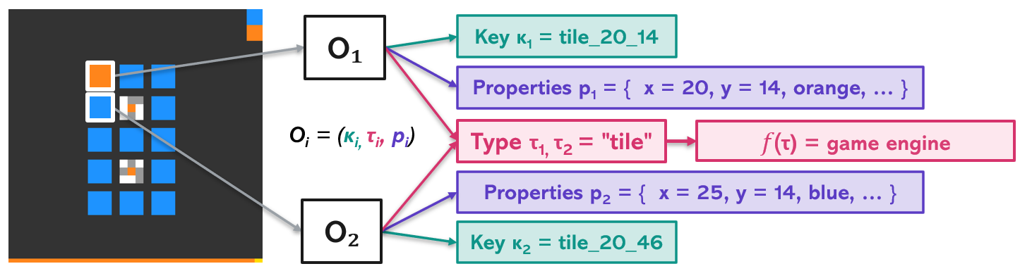
Thus the structured state at time \(t\) is written as a finite collection of objects: \[s_t=\{o_t^i:i\in I_t\}.\] Each object is written as \[o_t^i=(\kappa_t^i,\tau_t^i,\mathbf{v}_t^i).\]
| Symbol | Meaning in the ARC-3 example |
|---|---|
| \(s_t\) | all objects/sprites in the state at time \(t\) |
| \(I_t\) | object indices present at time \(t\) |
| \(o_t^i\) | object \(i\), e.g. the blue player or red key |
| \(\kappa_t^i\) | object key or matching cue, e.g. an engine sprite name |
| \(\tau_t^i\) | object type/tag/role, e.g. \(\text{\normalfont\ttfamily blue\_player}\) |
| \(\mathbf{v}_t^i\) | finite attribute valuation, e.g. \(x,y,\text{\normalfont\ttfamily visible},\text{\normalfont\ttfamily pixels}\) |
Here \(\mathbf{v}_t^i\) is the object’s finite attribute valuation. We use \(\mathbf{v}\), rather than \(\mathbf{p}\), to avoid conflict with probability notation later.
For an object of type \(\tau_t^i\), the attribute valuation is a finite map \[\mathbf{v}_t^i: \mathsf{Attr}(\tau_t^i)\to \mathsf{Val}.\] For an attribute \(b\in\mathsf{Attr}(\tau_t^i)\), we write \[\mathbf{v}_t^i(b)\] for its value. For ARC-3 sprites, attributes may include \[\mathsf{Attr}(\tau) = \{ \text{\normalfont\ttfamily x}, \text{\normalfont\ttfamily y}, \text{\normalfont\ttfamily visible}, \text{\normalfont\ttfamily rotation}, \text{\normalfont\ttfamily pixels}, \ldots \}.\]
15.2 Abstraction from raw observation to object state↩︎
The raw observation is denoted \(x_t\). In the sprite-based setting, \(x_t\) may already contain engine sprite records. In the spriteless setting, \(x_t\) may be only the grid or rendered frame. In both cases, the learner operates on an object-structured state, so we define an abstraction map \[\alpha:x_t\mapsto s_t\in\mathcal{S}.\]
| Symbol | Meaning |
|---|---|
| \(x_t\) | raw observation, e.g. grid, frame, or engine observation |
| \(\alpha\) | abstraction map from raw observation to object state |
| \(s_t=\alpha(x_t)\) | object-structured state used by the learner |
| \(\mathsf{Attr}(\tau)\) | attribute names available for type \(\tau\) |
| \(\mathbf{v}_t^i(b)\) | value of attribute \(b\) for object \(i\) at time \(t\) |
Importantly, \(\alpha\) is responsible not only for decomposing the observation into objects, but also for assigning the object-level fields used later by the learner: the matching cue \(\kappa_t^i\), the type/tag \(\tau_t^i\), and the attribute valuation \(\mathbf{v}_t^i\).
15.2.0.1 Given sprite abstraction.
In the current sprite-based implementation, object records are not inferred by the LLM. They come directly from the ARC engine. The adapter reads the current level’s sprite list and stores fields such as name, tags,
x, y, visible, rotation, and pixels. Thus \[\alpha_{\rm sprite}(x_t)=s_t\] is a deterministic engine-provided abstraction. In this regime, the object
decomposition, object type/tag, and name-based matching cue are all provided by the engine representation.
A sprite record may look like:
{
  "name": "spr_17",
  "tags": ["blue_player"],
  "x": 2,
  "y": 2,
  "visible": true,
  "rotation": 0,
  "pixels": [[1,1],[1,1]]
}
This record corresponds to \[o_t^i=(\kappa_t^i,\tau_t^i,\mathbf{v}_t^i),\] where \[\kappa_t^i=\text{\normalfont\ttfamily spr\_17}, \qquad \tau_t^i=\text{\normalfont\ttfamily blue\_player},\] and \[\mathbf{v}_t^i = \{ \text{\normalfont\ttfamily x}\mapsto 2,\; \text{\normalfont\ttfamily y}\mapsto 2,\; \text{\normalfont\ttfamily visible}\mapsto \text{\normalfont\ttfamily true},\; \text{\normalfont\ttfamily rotation}\mapsto 0,\; \text{\normalfont\ttfamily pixels}\mapsto \begin{bmatrix} 1 & 1\\ 1 & 1 \end{bmatrix} \}.\] Equivalently, after fixing an attribute order, this valuation can be written as a vector: \[\mathbf{v}_t^i = \left( 2,\; 2,\; \text{\normalfont\ttfamily true},\; 0,\; \begin{bmatrix} 1 & 1\\ 1 & 1 \end{bmatrix} \right).\] The dictionary view is usually clearer because ARC-3 attributes are heterogeneous.
15.2.0.2 Inferred object abstraction.
In the spriteless regime, the LLM must infer an object decomposition from the raw grid or frame. The output of \(\alpha_{\rm LLM}\) is still required to be a structured state \[s_t=\{o_t^i:i\in
I_t\}, \qquad o_t^i=(\kappa_t^i,\tau_t^i,\mathbf{v}_t^i).\] In this case, the construction of object keys is part of the inferred abstraction problem. In the current implementation, \(\alpha_{\rm LLM}\) is a
synthesized extract_objects(frame) function. Each object it returns carries its own name, id, or key field, used as the key \(\kappa_t^i\); when none is present, the key
defaults to \(\text{\normalfont\ttfamily type}\_\text{\normalfont\ttfamily index}\), the object type joined with its enumeration index in the frame. The type \(\tau_t^i\) is read from the
object’s type, kind, role, or tag field, defaulting to \(\text{\normalfont\ttfamily visual\_object}\). Once these keys are assigned, the pairing policy reuses the sprite
pairing heuristic below.
Remark 1 (Reported configuration). The experiments accompanying this paper are run in the spriteless regime: object records are produced by the synthesized extract_objects (\(\alpha_{\rm
LLM}\)), and all pairing, effect-count, and ontology-error diagnostics below are computed over those inferred records. The sprite-based descriptions are retained for exposition as the engine-given special case in which \(\alpha\) is provided rather than inferred.
15.3 Pairing objects across time↩︎
In Figure 13, imagine the player moves one cell to the right. The object in the next frame should still be recognized as the same player. Before we can say what changed, we need to pair before-objects in \(s_t\) with after-objects in \(s_{t+1}\).
We write the before/after matching as a partial map \[\mu_t:I_t\to I_{t+1}\cup\{\bot\}.\] If \(\mu_t(i)=i'\), then before-object \(o_t^i\) is paired with after-object \(o_{t+1}^{i'}\). If \(\mu_t(i)=\bot\), then object \(i\) is treated as disappeared.
| Symbol | Meaning |
|---|---|
| \(\mu_t\) | partial matching from before-objects to after-objects |
| \(\bot\) | no matched after-object; object disappeared |
| \(I_t\) | object indices present before the transition |
| \(I_{t+1}\) | object indices present after the transition |
In the current sprite-based implementation, pairing is not inferred by the LLM. It is a deterministic two-pass heuristic over engine-provided sprite records:
Group after-objects by their
name.First pair unused before/after objects with exact \[(\text{\normalfont\ttfamily name},x,y)\] matches.
For each remaining unmatched before-object, greedily pair it with the first unused after-object with the same
name, even if its position has changed.If no unused after-object with the same
nameremains, pair the before-object with \(\bot\). This produces the effect signature \[\text{\normalfont\ttfamily gone}.\]
This handles simple movement: an object that changes position fails the exact \((\text{\normalfont\ttfamily name},x,y)\) pass but can still be matched by the same-name pass. However, the method is still
heuristic. Sprite names are not guaranteed to be unique, and if multiple same-name sprites move simultaneously, greedy same-name matching can be ambiguous.
After-only objects are not currently emitted as separate effect-count samples by this pairing loop. They still appear in the full after-state \(s_{t+1}\), so they are visible to the transition verifier. If the Bayesian effect table is extended to count births, the natural signature is \[\text{\normalfont\ttfamily born},\] counted under the after-object’s type with context evaluated at the spawn location.
15.3.0.1 Spriteless pairing.
In the spriteless setting, the synthesized abstraction \(\alpha_{\rm LLM}\) first extracts object records from each frame, and then the same two-pass heuristic above is run over those records. The only difference is the
source of the key \(\kappa_t^i\). In sprite mode it is the engine sprite name; in spriteless mode it is the name, id, or key field emitted by extract_objects,
or a \(\text{\normalfont\ttfamily type}\_\text{\normalfont\ttfamily index}\) fallback when the synthesizer emits none. The exact-position pass still pairs stationary objects, and the same-name pass still recovers moved
objects, provided the synthesized extractor assigns keys consistently across frames. The same effect-count tables and ontology-error diagnostics are then produced in both modes.
16 Effect Signatures↩︎
In the grid example, once the player before the action is paired with the player after the action, we can ask what changed. If the player moved right, the \(\text{\normalfont\ttfamily x}\) attribute changed. If the player also changed appearance, then both \(\text{\normalfont\ttfamily x}\) and \(\text{\normalfont\ttfamily pixels}\) changed. This motivates a coarse object-level effect signature (Figure 2).
For a persistent object \(i\), where \(\mu_t(i)\neq\bot\), define the changed-attribute set \[\Delta_t^i = \left\{ b\in\mathsf{Attr}(\tau_t^i): \mathbf{v}_{t+1}^{\mu_t(i)}(b)\neq \mathbf{v}_t^i(b) \right\}.\] The effect signature is a finite categorical symbol: \[e_t^i=\rho(\Delta_t^i)\in\mathcal{E}.\]
| Symbol | Meaning |
|---|---|
| \(\Delta_t^i\) | set of object attributes that changed |
| \(\rho\) | quotient map from changed-attribute sets to effect signatures |
| \(e_t^i\) | effect signature for object \(i\) at time \(t\) |
| \(\mathcal{E}\) | finite effect-signature alphabet |
If an object disappears, so that \(\mu_t(i)=\bot\), the current implementation assigns \[e_t^i=\text{\normalfont\ttfamily gone}.\] After-only objects appear in \(s_{t+1}\) and are checked by the full transition verifier, but the current Bayesian effect-count loop does not emit them as separate birth samples. A natural extension is to add \[e_t^b=\text{\normalfont\ttfamily born}\] for after-only objects \(b\), counted under the after-object’s type.
The signature records which attributes changed, not the exact new values. For example, \(\text{\normalfont\ttfamily x}\) means the \(x\)-attribute changed, but does not say whether the object moved left or right. The exact next-state values remain in the full transition pair \((s_t,a_t,s_{t+1})\).
16.0.0.1 Example.
If the player moves right and changes its pixels, then \[\Delta_t^i=\{\text{\normalfont\ttfamily x},\text{\normalfont\ttfamily pixels}\},\] and the implementation may represent the signature as \[e_t^i=\text{\normalfont\ttfamily pixels,x}.\] This whole string is one categorical outcome. It is not treated as two independent Bernoulli observations.
17 Object-Lifted Transition Rules↩︎
In the grid example, the player should not need a separate transition rule at every absolute board location. Instead, the same type-level rule can apply to all player instances, with behavior depending on local context. For example, the action \(\text{\normalfont\ttfamily right}\) may move the player if the right cell is empty, and may do nothing if a wall is on the right.
The environment transition is still the ordinary MDP transition: \[T:\mathcal{S}\times\mathcal{A}\to\mathcal{S}.\] For a persistent object \(i\), where \(\mu_t(i)\neq\bot\), the lifted hypothesis class shares transition rules by type: \[o_{t+1}^{\mu_t(i)} \approx f_{\tau_t^i}(o_t^i,a_t,u_t^i).\] Here \[u_t^i=\psi(o_t^i,s_t)\] is the local context or state-feature value used by the object rule.
| Symbol | Meaning |
|---|---|
| \(T\) | true environment transition over full states |
| \(f_\tau\) | transition rule shared by objects of type \(\tau\) |
| \(\psi\) | state-feature/context map |
| \(u_t^i=\psi(o_t^i,s_t)\) | local feature value for object \(i\) at time \(t\) |
The word “lifted” means that \(f_\tau\) is a type-level rule, not a separate rule for every object instance. Grounding the rule on object \(o_t^i\) gives the object-level prediction.
17.0.0.1 Example.
For a player object with \(\tau_t^i=\text{\normalfont\ttfamily blue\_player}\), action \(\text{\normalfont\ttfamily right}\), and local context \(u_t^i=\text{\normalfont\ttfamily empty\_right}\), the rule may predict that \(\text{\normalfont\ttfamily x}\) changes. If instead \(u_t^i=\text{\normalfont\ttfamily wall\_right}\), the same action may produce no change. Thus the context \(u_t^i\) explains why the same type and action can have different effects in different local states.
18 The Local Effect Table↩︎
The grid example also motivates a count table. If the player takes \(\text{\normalfont\ttfamily right}\) several times, we can count what effect was observed under each local context. This table is not the executable transition model \(T\), and it is not the synthesized model \(\widehat T\). It is a local diagnostic summarizing how objects of a given type change under an action and context.
A table row is indexed by \[j=(\tau,a,u),\] where \(\tau\) is an object type, \(a\) is an action, and \(u\) is a local context feature. The columns are effect signatures \(e\in\mathcal{E}\). Thus the table has entries \[C_t(j,e)\in\mathbb{N}.\]
| Symbol | Meaning |
|---|---|
| \(j=(\tau,a,u)\) | row key: type, action, and local context |
| \(\mathcal{E}\) | finite set of effect-signature columns |
| \(C_t(j,e)\) | number of times row \(j\) produced effect \(e\) by time \(t\) |
| \(q_j(e)\) | categorical probability of effect \(e\) in row \(j\) |
For each real transition \((s_t,a_t,r_t,s_{t+1})\), and for each paired object \(i\), the system computes \[u_t^i=\psi(o_t^i,s_t),\] then assigns the object transition to the row \[j_t^i=(\tau_t^i,a_t,u_t^i).\] It also computes the observed effect signature \[e_t^i=\rho(\Delta_t^i).\] The table update is \[C_{t+1}(j,e) = C_t(j,e) + \sum_{i\in I_t} \mathbf{1}\{j_t^i=j,\;e_t^i=e\}.\] Equivalently, each object-level observation increments the cell \[C_t(j_t^i,e_t^i).\]
18.0.0.1 Example before context refinement.
The effect signature \(e_t^i\) is computed after the transition from \(\Delta_t^i\). The context feature \(u_t^i\) is computed before the transition from \(s_t\) and is used to define or split the row.
Suppose we initially use a coarse context value \(u_0\) for the player under action \(\text{\normalfont\ttfamily right}\). The local effect table may contain the following row.
| Type \(\tau\) | Action \(a\) | Context \(u\) | \(\text{\normalfont\ttfamily no\_change}\) | \(\text{\normalfont\ttfamily x}\) | \(\text{\normalfont\ttfamily pixels,x}\) | \(\text{\normalfont\ttfamily gone}\) |
|---|---|---|---|---|---|---|
| \(\text{\normalfont\ttfamily blue\_player}\) | \(\text{\normalfont\ttfamily right}\) | \(u_0\) | 2 | 3 | 0 | 0 |
This row is mixed: sometimes the player changes \(x\), and sometimes nothing changes. In a deterministic MDP, this usually means that the context feature is too coarse. For example, the missing feature may be the object type at offset \((1,0)\), i.e., whether there is empty space or a wall to the right.
After adding this feature, the same observations are split into two refined rows:
| Type \(\tau\) | Action \(a\) | Context \(u\) | \(\text{\normalfont\ttfamily no\_change}\) | \(\text{\normalfont\ttfamily x}\) | \(\text{\normalfont\ttfamily pixels,x}\) | \(\text{\normalfont\ttfamily gone}\) |
|---|---|---|---|---|---|---|
| \(\text{\normalfont\ttfamily blue\_player}\) | \(\text{\normalfont\ttfamily right}\) | \(\text{\normalfont\ttfamily empty\_right}\) | 0 | 3 | 0 | 0 |
| \(\text{\normalfont\ttfamily blue\_player}\) | \(\text{\normalfont\ttfamily right}\) | \(\text{\normalfont\ttfamily wall\_right}\) | 2 | 0 | 0 | 0 |
Both refined rows are concentrated. This is what context refinement checks: not whether a new effect exists, but whether a before-state feature explains why different effects were observed under the same type and action.
18.0.0.2 Example with a joint effect signature.
The table can also contain joint changed-attribute signatures. For instance, if a key-like sprite sometimes moves and changes pixels, its row may contain a nonzero count in the \(\text{\normalfont\ttfamily pixels,x}\) column:
| Type \(\tau\) | Action \(a\) | Context \(u\) | \(\text{\normalfont\ttfamily no\_change}\) | \(\text{\normalfont\ttfamily x}\) | \(\text{\normalfont\ttfamily pixels,x}\) | \(\text{\normalfont\ttfamily gone}\) |
|---|---|---|---|---|---|---|
| \(\text{\normalfont\ttfamily red\_key}\) | \(\text{\normalfont\ttfamily right}\) | \(\text{\normalfont\ttfamily near\_player}\) | 1 | 0 | 2 | 0 |
The entry \(\text{\normalfont\ttfamily pixels,x}\) is one categorical outcome. It is not treated as an independent \(\text{\normalfont\ttfamily pixels}\) change plus an independent \(\text{\normalfont\ttfamily x}\) change.
19 Dirichlet Row Diagnostics↩︎
The local effect table gives counts. To measure whether a row is stable, we place a categorical distribution over effect signatures on each row: \[q_j(e)=\Pr(e_t^i=e\mid j_t^i=j).\] Let \[\mathcal{E}=\{e_1,\ldots,e_m\}.\] The count vector for row \(j\) is \[\mathbf{c}_j = (C_t(j,e_1),\ldots,C_t(j,e_m)).\] We place a symmetric Dirichlet prior: \[q_j\sim\mathop{\mathrm{Dir}}(\alpha_0\mathbf{1}_m).\] By conjugacy, \[q_j\mid\mathcal{D}_t \sim \mathop{\mathrm{Dir}}(\alpha_0\mathbf{1}_m+\mathbf{c}_j).\] The posterior mean is \[\widehat q_j(e) = \frac{\alpha_0+C_t(j,e)}{m\alpha_0+\sum_{e'}C_t(j,e')}.\]
| Symbol | Meaning |
|---|---|
| \(q_j(e)\) | row-level categorical probability of effect \(e\) |
| \(\mathbf{c}_j\) | count vector for row \(j\) |
| \(\alpha_0\) | Dirichlet pseudo-count |
| \(\widehat q_j(e)\) | posterior-mean probability of effect \(e\) in row \(j\) |
The Dirichlet posterior is not the world model. It only summarizes which attributes changed. The executable transition model is still \[\widehat T:\mathcal{S}\times\mathcal{A}\to\mathcal{S},\] and it must satisfy full next-state replay constraints: \[\widehat T(s_t,a_t)=s_{t+1}.\]
20 Row Concentration and Context Refinement↩︎
The mixed player row from Section 18 illustrates the purpose of row concentration. If the row contains both \(\text{\normalfont\ttfamily x}\) and \(\text{\normalfont\ttfamily no\_change}\), then the current type-action-context condition is not specific enough. A refined context feature, such as whether the right neighbor is empty or a wall, can split the row into deterministic subrows (Figure 3).
The number of samples assigned to row \(j\) is \[n_j=\sum_{e\in\mathcal{E}}C_t(j,e),\] and the modal count is \[s_j=\max_{e\in\mathcal{E}}C_t(j,e).\] The modal fraction is \[\mathrm{modal\_frac}(j)=\frac{s_j}{n_j}, \qquad n_j>0.\]
A row is operationally identified when \[n_j\ge n_{\min}, \qquad \mathrm{modal\_frac}(j)\ge m_{\min}.\] The full row uncertainty can also be measured by normalized entropy: \[U_j^{\rm row} = \frac{\mathsf H(\widehat q_j)}{\log m} \in[0,1].\]
| Symbol | Meaning |
|---|---|
| \(n_j\) | number of samples assigned to row \(j\) |
| \(s_j\) | count of the most common effect in row \(j\) |
| \(\mathrm{modal\_frac}(j)\) | empirical concentration of the row |
| \(U_j^{\rm row}\) | normalized entropy of the row’s effect distribution |
Returning to the example in Section 18, the coarse row \[j=(\text{\normalfont\ttfamily blue\_player},\text{\normalfont\ttfamily right},u_0)\] has \[C_t(j,\text{\normalfont\ttfamily x})=3, \qquad C_t(j,\text{\normalfont\ttfamily no\_change})=2.\] Thus \[n_j=5, \qquad s_j=3, \qquad \mathrm{modal\_frac}(j)=\frac{3}{5}.\] This row is not concentrated. After adding the right-neighbor context feature, the refined row \[j_1=(\text{\normalfont\ttfamily blue\_player},\text{\normalfont\ttfamily right},\text{\normalfont\ttfamily empty\_right})\] has \[C_t(j_1,\text{\normalfont\ttfamily x})=3, \qquad n_{j_1}=3, \qquad \mathrm{modal\_frac}(j_1)=1,\] and the refined row \[j_2=(\text{\normalfont\ttfamily blue\_player},\text{\normalfont\ttfamily right},\text{\normalfont\ttfamily wall\_right})\] has \[C_t(j_2,\text{\normalfont\ttfamily no\_change})=2, \qquad n_{j_2}=2, \qquad \mathrm{modal\_frac}(j_2)=1.\] The split is useful because a before-state context feature explains the mixed effects in the original row. In the implementation, minimum-count thresholds may still require additional samples before a refined row is accepted as identified.
21 Typing Uncertainty↩︎
In the running grid, \(\text{\normalfont\ttfamily blue\_player}\) and \(\text{\normalfont\ttfamily red\_key}\) are useful initial types. But in the general case, the observed tag may not be the true mechanical role, or the object decomposition may be inferred from pixels. The learner therefore maintains uncertainty over candidate mechanical types: \[\tau_t^i\in\mathcal{C}=\{1,\ldots,K\}.\]
The analyzer or LLM supplies a prior: \[\pi_i(\tau)=\Pr(\tau_t^i=\tau).\] For a candidate type \(\tau\), object \(i\)’s row at time \(t\) would be \[j_t^i(\tau)=(\tau,a_t,u_t^i).\] The plug-in likelihood of the observed effect is \[\ell_t^i(\tau) = \widehat q_{j_t^i(\tau)}(e_t^i).\] Thus an approximate type posterior is \[\Pr(\tau_t^i=\tau\mid\mathcal{D}_t) \propto \pi_i(\tau) \prod_{\ell<t:\,i\in I_\ell} \ell_\ell^i(\tau).\]
| Symbol | Meaning |
|---|---|
| \(\mathcal{C}\) | finite candidate type set |
| \(\pi_i(\tau)\) | analyzer/LLM prior that object \(i\) has type \(\tau\) |
| \(j_t^i(\tau)\) | row assignment under candidate type \(\tau\) |
| \(\ell_t^i(\tau)\) | plug-in likelihood of observed effect under type \(\tau\) |
In the current ARC-3 implementation, this posterior may be shared per sprite tag rather than stored independently for every object instance. That is, all objects with the same engine tag share the same type posterior.
The normalized typing uncertainty is \[U_i^{\rm type} = \frac{ \mathsf H[\Pr(\tau_t^i\mid\mathcal{D}_t)] }{\log K} \in[0,1].\]
22 Ontology Error↩︎
The local table can be uncertain for two different reasons. First, the system may be unsure which type governs an object. Second, even after choosing a type, the row may still mix multiple effects. Ontology error combines these two sources of uncertainty.
For object \(i\) assigned to row \(j_t^i\), define \[\eta_t^i = 1- (1-U_i^{\rm type}) (1-U_{j_t^i}^{\rm row}).\] This noisy-OR score is high if either the object type is uncertain or the row is uncertain. It is low only when both are resolved.
The aggregate ontology error is \[\eta_t = \frac{1}{N_t} \sum_{\ell<t} \sum_{i\in I_\ell} \eta_\ell^i,\] where \[N_t=\sum_{\ell<t}|I_\ell|.\]
| Symbol | Meaning |
|---|---|
| \(U_i^{\rm type}\) | uncertainty about object \(i\)’s type |
| \(U_{j_t^i}^{\rm row}\) | uncertainty about the row’s effect distribution |
| \(\eta_t^i\) | object-row ontology error |
| \(\eta_t\) | aggregate ontology error |
If \(U_i^{\rm type}\) is high, the system is unsure which type/role should govern object \(i\). If \(U_{j_t^i}^{\rm row}\) is high, the row mixes several effect signatures, which often means that the local context \(u_t^i\) is missing a relevant feature or that the current type groups together heterogeneous objects.
Ontology error does not say that all world-model errors are typing or row errors. The synthesized transition code can still be wrong in exact values, pairing can be wrong, the abstraction \(\alpha\) can miss objects, or the goal predicate can be wrong. Those failures are caught by replay verification, not by ontology error alone.
Remark 2 (Role of the diagnostic). The ontology error is, and is used as, a compact correlational exploration signal. It is computed from effect signatures \(\rho(\Delta_t^i)\), which record which* attributes changed and discard the exact deltas; a concentrated row is therefore strong evidence of—though not a proof of—a determinate transition, the exact values being resolved by the synthesized code. Its role is to direct search cheaply: a high \(\eta_t^i\) marks the objects and contexts where the action agent should explore next and the synthesizer should refine typing or local context, while a falling \(\eta_t\) tracks the ontology settling (Figure 4). Correctness of the world model is decided not by \(\eta\) but by the full-state replay verifier \(\phi_T\) (Section 24); the diagnostic and the verifier are complementary—\(\eta\) is a fast, fuzzy guide, \(\phi_T\) the exact criterion.*
23 Crystallization↩︎
The previous sections define uncertainty signals. Crystallization is the point where the system decides that the object ontology is stable enough to commit to a synthesized model.
Let \(\mathcal{I}^G\) be the set of goal-relevant objects, tags, or groups, estimated after the first successful trajectory. An idealized crystallization time is \[t^\star = \min \left\{ t: \begin{array}{l} \text{some reward } r_\ell=1 \text{ has been observed for } \ell<t,\\[1mm] U_i^{\rm type}\le \epsilon_{\rm type} \text{ for all goal-relevant objects } i,\\[1mm] n_j\ge n_{\min} \text{ and } \mathrm{modal\_frac}(j)\ge m_{\min} \text{ for all visited goal-relevant rows }j. \end{array} \right\}.\] At \(t^\star\), the system commits to the current ontology and asks the synthesizer for a stable executable model.
In the current ARC-3 implementation, the operational trigger is simpler: successful level completion plus confident non-decorative aliases. The stricter row gate is best viewed as a general design target.
24 Synthesized World Model↩︎
After commitment, the goal is not merely to know that a row usually changes \(\text{\normalfont\ttfamily x}\). The system must synthesize executable code that predicts the full next state. Therefore the learned world
model is \[\widehat T:\mathcal{S}\times\mathcal{A}\to\mathcal{S}, \qquad \widehat G:\mathcal{S}\times\mathcal{A}\times\mathcal{S}\to\{0,1\}.\] In code, \(\widehat T\) is implemented as
transition_function(state, action_id), and \(\widehat G\) is implemented as reward_function(state, action_id, new_state).
The transition verifier checks \[\phi_T(\widehat T,\mathcal{D}_t): \qquad \forall (s_\ell,a_\ell,r_\ell,s_{\ell+1})\in\mathcal{D}_t,\; \widehat T(s_\ell,a_\ell)=s_{\ell+1}.\] After positive rewards exist, the goal verifier checks \[\phi_G(\widehat G,\mathcal{D}_t): \qquad \forall (s_\ell,a_\ell,r_\ell,s_{\ell+1})\in\mathcal{D}_t,\; \widehat G(s_\ell,a_\ell,s_{\ell+1})=r_\ell.\]
A failed prediction, \[\widehat T(s_t,a_t)\neq s_{t+1},\] is a counterexample for the next synthesis round. It is also a real transition and therefore updates the Bayesian diagnostics through the same effect-count mechanism.
25 Planning and Model Use↩︎
If a reliable model has been synthesized, it can be used for model-based planning. A planner searches inside the learned model \[\widehat M=(\mathcal{S},\mathcal{A},\widehat T,\widehat G).\] Given the current observed state \(s_t\), it returns a predicted trace \[\widehat\tau = (\widehat s_t,a_t,\widehat s_{t+1},a_{t+1},\ldots,\widehat s_{t+L}),\] where \[\widehat s_t=s_t, \qquad \widehat s_{k+1}=\widehat T(\widehat s_k,a_k).\] The first action of the trace gives the planner-induced policy: \[\pi_{\rm plan}(s_t)=a_t.\]
Execution still occurs in the real environment. If the real next state differs from the predicted next state, the transition becomes a counterexample: \[s_{t+1}\neq \widehat T(s_t,a_t).\] Thus model use and real-environment validation remain separate.
The current codebase implements such a planner as a synthesized module. The synthesizer authors a planner hook that searches over its own transition_function and reward_function for an action sequence that reaches
reward under the model. The planner runs only after at least one level has been completed and after the synthesized model is replay-consistent, and it is first verified by planning to reward from the entry states of the completed levels before it is
trusted. Each planned action is then executed one step at a time in the real environment and compared against the predicted next state. A mismatch aborts the plan, appends the real transition to the replay buffer as a counterexample, and blocks the planner
until the next synthesis round. The planner is a tool the action agent may consult, while the action agent still selects every move and checks model consistency through the replay buffer.
26 Division of Labor: Actor, Synthesizer, and Critic↩︎
Control and model construction are separated across two LLM-driven roles that share one symbolic world model \(\widehat M=(\mathcal{S},\mathcal{A},\widehat T,\widehat G)\).
26.0.0.1 Actor.
The actor selects the primitive action \(a_t\) executed in the real environment at each step and records every real transition \((s_t,a_t,r_t,s_{t+1})\) in the replay buffer \(\mathcal{D}_t\). When a trusted model exists it may follow the planner-induced policy \(\pi_{\rm plan}\) (Section 25), but it selects every move itself.
26.0.0.2 Synthesizer.
The synthesizer authors and repairs \(\widehat T\), \(\widehat G\), and the planner. Repair is counterexample-guided: any transition in \(\mathcal{D}_t\) on which the verifier \(\phi_T\) or \(\phi_G\) (Section 24) fails is a counterexample for the next synthesis round.
26.0.0.3 Critic.
A critic call audits the current model against the buffer and the diagnostics of Section 22, surfacing the counterexamples and the high-\(\eta\) objects and contexts that the next synthesis round should address. The critic scores the consistency of the model with observed transitions, not the value of the actor’s actions.
26.0.0.4 Relation to actor–critic.
This is a model-based variant of the actor–critic pattern from reinforcement learning, with one substitution worth stating precisely. In standard actor–critic the critic is a learned value function that supplies the actor a low-variance reward signal. Here the only extrinsic reward is the sparse environment success \(R\) (reaching the goal); the critic instead scores the replay-consistency of a symbolic world model. Model consistency is thus an instrumental, intermediate objective: a model that replays the observed transitions is a prerequisite for planning to the sparse goal, so consistency acts as a dense signal in service of the terminal reward rather than an estimate of the policy’s value. Operationally the synthesizer first seeks and resolves inconsistencies—treating each mispredicted transition as a causal hypothesis to test against \(\mathcal{D}_t\)—and, once the model is replay-consistent, plans toward reward; the trade-off between further exploration and goal-seeking is handled heuristically rather than by an explicit objective. The artifact shared across all three roles is \(\widehat M\): the actor plans with it, the synthesizer repairs it, and the critic audits it, while the ontology error \(\eta_t\) (Section 22) is the compact signal that directs where each looks next.
27 Object-Based and Fluent-Based Views↩︎
The main formalization is object-based: \[s_t=\{o_t^i:i\in I_t\}, \qquad o_t^i=(\kappa_t^i,\tau_t^i,\mathbf{v}_t^i).\] This matches the implementation, which stores sprite/object records and computes object-level effect signatures.
The fluent-based view is a field-level expansion. If \(b\) is an attribute name in \(\mathsf{Attr}(\tau_t^i)\), then a grounded fluent is \[y=(i,b),\] meaning attribute \(b\) of object \(i\). Its value is \[s_t(y)=\mathbf{v}_t^i(b).\] The object transition is equivalent to a bundle of fluent transitions: \[\mathbf{v}_t^i(b) \mapsto \mathbf{v}_{t+1}^{\mu_t(i)}(b), \qquad b\in\mathsf{Attr}(\tau_t^i).\]
| Object-based view | Fluent-based view | |
|---|---|---|
| State carrier | Object \(o_t^i\) | Grounded attribute \(y=(i,b)\) |
| Transition unit | Object record update | Single attribute update |
| Row | \(j=(\tau,a,u)\) | \(j=(\tau,b,a,u)\) |
| Effect | Changed-attribute mask, e.g. x,y |
Attribute-level change/no-change |
| Best use | Current ARC-3 implementation | Connection to lifted/factored MDP notation |
We therefore use the object-based view as the main formalization and the fluent-based view only as an explanatory expansion.
28 Summary↩︎
The full flow is: \[x_t \xrightarrow{\alpha} s_t=\{o_t^i:i\in I_t\}, \qquad o_t^i=(\kappa_t^i,\tau_t^i,\mathbf{v}_t^i).\] The real environment transition gives \[s_{t+1}=T(s_t,a_t).\] The system pairs objects across \(s_t\) and \(s_{t+1}\), computes effect signatures \(e_t^i\), assigns local effect-table rows \[j_t^i=(\tau_t^i,a_t,u_t^i),\] updates Dirichlet row diagnostics, updates type uncertainty, and computes ontology error. When the ontology is stable enough, the system commits and synthesizes an executable world model \(\widehat T\). The Bayesian diagnostic tracks row-level abstraction adequacy; the executable model is checked by full next-state equality.