The risk of KV cache compression
July 01, 2026
Abstract
Transformer inference on long sequences is expensive because softmax attention repeatedly reads from a large KV cache. The prevalent approach to this bottleneck is KV cache compression, which replaces the full cache with a compact summary. Despite its practical importance, the design of such summaries is largely driven by empirical experimentation. On the theoretical side, existing results show that KV cache compression can be impossible in the worst case, but offer little systematic guidance for designing algorithms in regimes where accurate compression is possible. We bridge this gap by characterizing the minimax risk of KV cache compression in terms of the intrinsic compressibility of a cache, revealing when and how accurate compression is possible. These results yield novel design principles for KV cache compression under causal masking that map efficiently to prefill and autoregressive decoding while achieving minimax-optimal risk. We instantiate these principles in a practical algorithm and report promising performance on LongBench in targeted experiments. Overall, our results provide a principled avenue for practical KV cache compression with theoretical guarantees.
1 Introduction↩︎
Transformers have become the dominant architecture for processing and generating long sequences across various domains [1]–[4] due to their excellent ability to model complex interactions between tokens. During inference, these interactions are mediated through the key–value (KV) cache storing all previous tokens, and each new token is computed from this cache via softmax attention [5]. The KV cache therefore serves as the model’s working memory of the past. While this persistent access to past data makes Transformers powerful, it is also costly. As the sequence grows, the cache grows with it, and each new step must read from an increasingly large history. For long-context applications, this creates a major bottleneck in both memory use and runtime.
An attractive remedy is KV compression: replacing a long history of key–value pairs by a compact summary that approximately preserves the attention outputs of the original cache.2 Such a summary is useful only if future attention cannot reliably distinguish the compressed cache from the full history. This makes it challenging to decide which distinctions in the past can be safely forgotten, because the importance of a token is not intrinsic to the token itself. A token that can be safely discarded in one context and for one set of future queries may be essential for another, while several distinct tokens may be interchangeable if attention uses them in the same way. Thus, compression is safe only to the extent that the summary preserves the context that future queries can actually use.
Despite its practical importance, KV compression lacks a systematic design theory and remains largely guided by empirical exploration [6]–[11], using heuristic proxies for future relevance such as recency, accumulated attention mass, and attention sinks. These methods show substantial compression is often possible, but they do not explain which properties of a cache make compression safe, how the achievable error should scale with the compression budget, or what an optimal summary should preserve. Conversely, theoretical results show that accurate KV compression can be impossible in the worst case [12], and identify structural assumptions under which compression is possible [13]–[15]. This leaves open the intermediate regime most relevant to practical algorithm design: caches that are not adversarial, but also not prescribed by a fixed model class.
To bridge this gap, we provide a graded account of KV cache compressibility in terms of the intrinsic interaction between a cache and future queries through softmax attention. Specifically, we characterize the minimax risk of KV compression, asking: for a fixed compression budget, how much error is unavoidable for the way a given cache can be probed by future queries? Beyond quantitative rates, this characterization identifies what an optimal summary must preserve. It captures the continuum between easy regimes, where many past tokens are effectively redundant and a small summary can preserve attention accurately, and hard regimes, where the cache contains many separately retrievable pieces of information and any small summary must lose something, and yields concrete design criteria for algorithms to attain minimax-optimal risk.
Concretely, we make the following contributions. (1) We recast KV compression as sparse approximation of a measure, strictly generalizing token eviction, and formalize its minimax risk. (2) We prove tight upper and lower bounds on this risk in terms of an intrinsic complexity measure capturing how future queries probe the cache, and show a sharp separation between algorithms with and without access to the future-query distribution. (3) We derive design principles for efficient KV compression during causally masked prefill and autoregressive decoding with minimax-optimal compression risk. (4) We instantiate these principles in a concrete KV compression algorithm and evaluate it through targeted experiments on LongBench, where it shows promising performance. Put together, our results advance KV compression towards practical methods with theoretical guarantees.
2 Related work↩︎
A large body of recent work reduces KV cache size by selecting tokens according to empirical proxies for future relevance. These proxies include recency and attention sinks [7], [8], accumulated or persistent attention mass [6], [7], [11], and attention patterns observed during prefill or across layers [9], [10]. The strong empirical performance of these methods suggests that real Transformer caches often contain substantial redundancy. At the same time, these proxies do not by themselves explain which properties of a cache make compression safe, how the achievable error should scale with the compression budget, or what information an optimal summary must preserve. Our work addresses this gap by studying the minimax risk of KV compression algorithms broadly, aiming to inform practical compression beyond empirical exploration.
Existing theory has mainly identified two endpoints: impossibility results for sharp token retrieval [12], [16], and positive approximation guarantees under additional structure [13]–[15], [17]. These results identify important limitations and tractable regimes, but they do not give a graded characterization from lossless compression to worst-case incompressibility. Our upper bounds require no a priori structural model of the data beyond bounded values, which is weaker than bounded keys and queries. Instead, we deliberately characterize the compression risk through the interaction between caches and softmax attention itself. Our lower-bound assumptions are close in spirit to the sharp-attention regimes considered in prior hardness results. However, we employ them to characterize when compression remains possible, even under sharp attention, not to establish impossibility alone.
Finally, we formalize the minimax risk of KV compression as sparse approximation of a measure. Measure-based views of softmax attention and Transformers are not new, and have led to useful perspectives in several settings [18], [19]. To the best of our knowledge, our recasting is new for KV compression, and it strictly generalizes token eviction from subset selection to sparse reweighting.
3 Problem setup↩︎
We study KV compression: the problem of replacing the context seen by a single softmax attention head with a compact summary while preserving its outputs on future queries, in order to reduce memory use and computational cost. Since softmax attention depends on the context only through the induced weighting of its key–value pairs, we formalize KV compression as sparse approximation of a probability measure over tokens. Our goal is to characterize the achievable error for this approximation problem as a function of the context’s intrinsic compressibility under a query distribution, which we formalize as a minimax risk in terms of a data-dependent complexity measure.
3.1 KV compression as sparse approximation of a probability measure↩︎
In their seminal work, [5] define softmax attention as \[\label{eq:attention-standard} \mathop{\mathrm{Att}}\bigl(q \mid k_1, \dots, k_n, v_1, \dots, v_n\bigr) = \frac{ \sum_{i=1}^n \exp\left(\left\langle q, k_i \right\rangle/\sqrt{d_k}\right) \, v_i }{ \sum_{i=1}^n \exp\left(\left\langle q, k_i \right\rangle/\sqrt{d_k}\right) },\tag{1}\] where \(q\in\mathcal{Q}\) is a query, \(k_i\in\mathcal{K}\) are keys, and \(v_i \in\mathcal{V}\) are values, in their respective spaces \(\mathcal{K},\mathcal{Q}\subseteq \mathbb{R}^{d_k}\) and \(\mathcal{V}\subseteq \mathbb{R}^{d_v}\). We write \(\mathcal{X}\mathrel{\vcenter{:}}= \mathcal{K}\times \mathcal{V}\) for the key–value space, and assume throughout that values are bounded in norm by a constant \(V > 0\), which is usually not restrictive in practice.
The collection \((k_i,v_i)_{i=1}^n\) of key–value pairs in 1 is called the KV cache. We study the problem of KV compression: finding a compact representation of this collection that approximately preserves the attention map in 1 . Since 1 depends on the KV cache only through a weighted combination, we represent the KV cache as a finitely supported probability measure \(P\) and define \[\label{eq:attention} \att*{q}{P} \mathrel{\vcenter{:}}= \int_{\mathcal{X}} a_k(q \mid P)\, v \, \mathop{}\!\mathrm{d}P(k,v), \qquad a_k(q \mid P) \mathrel{\vcenter{:}}= \frac{\kappa(q,k)}{\int_{\mathcal{X}} \kappa(q,k') \, \mathop{}\!\mathrm{d}P(k',v')}\tag{2}\] for a Gaussian kernel \(\kappa(q,k) \mathrel{\vcenter{:}}= \exp(-\|q-k\|_2^2 / (2\sqrt{d_k}))\) on \(\mathbb{R}^{d_k}\) with scale parameter \(\sqrt{d_k}\). This definition coincides with 1 whenever \(P \propto \sum_{i=1}^n \exp\bigl(\|k_i\|^2 / (2\sqrt{d_k})\bigr) \cdot \delta_{(k_i,v_i)}\). For the remainder of this paper, we work with attention as defined in 2 so that attention depends on the KV cache only through the context measure \(P\).
To formalize KV compression from this viewpoint, we introduce the notation \(\mathcal{P}(\mathcal{S})\) for the probability measures on a subset \(\mathcal{S} \subseteq \mathcal{H}\) of a Hilbert space \(\mathcal{H}\), and denote by \(\mathcal{P}_\mathrm{fin}(\mathcal{S})\) those with finite support and by \(\mathcal{P}_K(\mathcal{S})\) those supported on at most \(K\) points. KV compression then becomes the following problem.
Given a budget \(K \ge 1\), a context measure \(P \in \kvmeasures\), and a query distribution \(\nu \in \mathcal{P}(\mathcal{Q})\), find a compressed context measure \(\hat{P} \in \kvmeasures[K]\) minimizing the mean squared error \[\textstyle \err*{P}{\nu}{\hat{P}} \mathrel{\vcenter{:}}= \mathop{\mathrm{\mathbb{E}}}_{q \sim \nu}\bigl\|\att*{q}{P} - \att*{q}{\hat{P}}\bigr\|_2^2.\]
[prb:kv-compression] strictly generalizes token eviction [6]–[10], which seeks a small, unweighted subset of \(K\) tokens that approximately preserve the attention map. In our setting, these tokens form the support of \(\hat{P}\). However, we allow arbitrary sparse reweightings of the cache, which, to the best of our knowledge, provides a new view on KV compression.
3.2 Capturing the intrinsic compressibility of a context↩︎
To understand when accurate compression is possible, we identify how changes to \(P\) affect softmax attention. Since \(P\) and \(\hat{P}\) are both probability measures, their difference \(\Delta \mathrel{\vcenter{:}}= \hat{P} - P\) is a signed, zero-mass measure. Compression can therefore be viewed as a reweighting of the original context, and its error is determined by how this reweighting perturbs the softmax numerator and normalizer.
Indeed, a direct computation shows that, for every query \(q \in \mathcal{Q}\), \[\label{eq:attention-reweighting} \att{q}{\hat{P}}-\att{q}{P} = \frac{ \int_\mathcal{X}a_k(q \mid P)\bigl(v-\att{q}{P}\bigr)\,\mathop{}\!\mathrm{d}\Delta(k,v) }{ 1+\int_\mathcal{X}\bigl(a_k(q \mid P)-1\bigr)\,\mathop{}\!\mathrm{d}\Delta(k,v) }.\tag{3}\] Thus, every compression perturbation enters attention through two linear functionals of \(\Delta\): a centered numerator term and a centered renormalization term. This identifies the pair of query-indexed coefficients with which each \((k,v) \in \mathcal{X}\) contributes to the compression-induced reweighting of tokens. We collect these coefficients with the following definition.
Definition 1 (Response profile). Let \(P \in \kvmeasures\) be a context measure and \(\nu \in \mathcal{P}(\mathcal{Q})\) a query distribution. We call \[\label{eq:response-profile} \Gamma_P(k,v) : \mathcal{Q}\to \mathbb{R}^{d_v}\oplus\mathbb{R}, \qquad q \mapsto \Bigl( a_k(q \mid P)\bigl(v-\att{q}{P}\bigr), \; V\bigl(a_k(q \mid P)-1\bigr) \Bigr)\qquad{(1)}\] the response profile* of \(P\). We view \(\Gamma_P(k,v)\) as an element of the Hilbert space \(\mathcal{H}_\nu \mathrel{\vcenter{:}}= L_2(\nu, \mathbb{R}^{d_v} \oplus \mathbb{R})\) and define the covariance operator \[\textstyle \Sigma_{P,\nu} \mathrel{\vcenter{:}}= \int_\mathcal{X}\Gamma_P(k,v) \otimes \Gamma_P(k,v) \,\mathop{}\!\mathrm{d}P(k,v).\]*
The first coordinate of \(\Gamma_P(k,v)\) records the token’s contribution to the centered numerator perturbation in 3 . The second coordinate records its contribution to the centered denominator perturbation, scaled by the value bound \(V\) so that both coordinates have the same units. The query distribution enters through the norm on \(\mathcal{H}_\nu\): Directions that matter on frequent queries are weighted heavily, while directions that matter only on rare queries are weighted lightly. Consequently, \(\Sigma_{P,\nu}\) measures the amount and geometry of query-visible variation in the context. While we do not claim that \(\Sigma_{P,\nu}\) is the only object to capture the intrinsic redundancy of a context, we argue that it is a meaningful choice. To substantiate this, we give three examples illustrating that the spectral decay of \(\Sigma_{P,\nu}\) tracks the intuitive difficulty of compression in several natural regimes.
exampleexpneedles Suppose a context \(P\) consists of \(m\) approximately equal “hay tokens” and \(n \ll m\) “needle tokens” that are well separated from all other tokens and dominate under \(\nu\). Then, \(\Sigma_{P,\nu}\) has few large eigenvalues.
exampleexpclusters Suppose a context \(P\) consists of \(m\) well-separated clusters of nearly interchangeable tokens, and the \(j\)-th cluster dominates under \(\nu\) with frequency of order \(j^{-(1+\alpha)}\). Then, the eigenvalues of \(\Sigma_{P,\nu}\) decay as \(r^{-\alpha}\).
exampleexplookup Suppose a context \(P\) consists of \(m\) pairwise well-separated tokens, and the query distribution \(\nu\) is diffuse. Then, \(\Sigma_{P,\nu}\) has many large eigenvalues.
3.3 Characterizing the achievable error of KV compression algorithms↩︎
Our goal in this paper is to characterize the fundamental limits of KV compression. Specifically, we seek minimax rates in terms of the intrinsic compressibility of a context by asking: What error does the best compression algorithm incur on its worst input \((P,\nu)\), as a function of \(\Sigma_{P,\nu}\)? To make this precise, we first specify what information a compression algorithm may use.
Definition 2 (Compressor). A \(K\)-compressor is a map \(A: \kvmeasures \times \mathcal{P}(\mathcal{Q})\times \Omega \to \kvmeasures[K]\) over a probability space \((\Omega,\mathcal{F},\mathbb{P})\) of random seeds. We write \(\compspace{K}\) for the class of all such compressors.
This definition allows compression algorithms to be randomized. It also allows the compressor to depend on the query distribution \(\nu\). We call this the query-aware setting. In many applications, however, the compressed summary must be formed before the future query distribution is known, which we call the query-agnostic setting, which we capture through the following restricted class.
Definition 3 (Query-agnostic compressor). We call a \(K\)-compressor \(A \in \compspace{K}\) query-agnostic if \(A(P,\nu,\omega) = A(P,\rho,\omega)\) for all \(\nu,\rho \in \mathcal{P}(\mathcal{Q})\), \(P \in \kvmeasures\), and \(\omega \in \Omega\). We write \(\compspace{K}[ag]\) for the class of all query-agnostic \(K\)-compressors.
We measure the performance of a class of compressors by its worst-case expected mean squared error over a prescribed family of contexts and query distributions.
Definition 4 (Minimax risk). Fix \(K \ge 1\). For a family of compressors \(\mathcal{C} \subseteq \compspace{K}\), and a family of context and query measures \(\mathcal{F} \subseteq \kvmeasures \times \mathcal{P}(\mathcal{Q})\), define the minimax compression risk \[\mathfrak{R}\!\left(\mathcal{C},\mathcal{F}\right) \mathrel{\vcenter{:}}= \inf_{A \in \mathcal{C}} \sup_{(P,\nu) \in \mathcal{F}} \mathop{\mathrm{\mathbb{E}}}_{\omega \sim \mathbb{P}}\!\left[ \err*{P}{\nu}{A(P, \nu, \omega)} \right].\]
Our objective is to characterize \(\mathfrak{R}\!\left(\compspace{K},\mathcal{F}\right)\) and \(\mathfrak{R}\!\left(\compspace{K}[ag],\mathcal{F}\right)\) through the response covariances \(\Sigma_{P,\nu}\) realized by \((P,\nu)\in\mathcal{F}\), and to use this characterization to identify what compressed summaries must preserve in order to attain minimax-optimal risk.
4 Minimax rates for KV compression↩︎
We now study the minimax risk of KV compression. 1 illustrates our approach: compressing a KV cache amounts to replacing the context measure \(P\) by a sparse reweighting, so that many tokens receive weight \(0\) while the remaining tokens are reweighted to preserve the effect of the full context on the attention map. To track this effect, we represent each key–value pair \((k,v)\in\mathcal{X}\) by its response profile \(\Gamma_P(k,v)\in\mathcal{H}_\nu\), which records the contribution of \((k,v)\) to the attention numerator and denominator under reweightings of \(P\). These individual contributions combine through their barycenter in \(\mathcal{H}_\nu\). As we show, reweightings causing small barycenter displacement also cause small attention error, recasting KV compression as a balancing problem in Hilbert space: given a context measure \(P\), reweight \(P\) so that its support is limited to at most \(K\) tokens while the barycenter of the response profiles remains nearly fixed. [prb:barycenter-sparsification] formulates this problem abstractly.
None
Figure 1: Illustration of our approach. Left: We view the token sequence as a measure \(P\) over key–value pairs \((k,v) \in \mathcal{X}\), which we map to their response profiles \(\Gamma_P(k,v) \in \mathcal{H}_\nu\). Right: Compressing \(P\) amounts to a sparse reweighting of tokens, which moves the barycenter of the response profiles. The size of this displacement depends on the retained tokens and their assigned weights, and controls the attention error incurred by compression. KV compression therefore reduces to a balancing problem in Hilbert space: find a \(K\)-atomic reweighting that keeps the barycenter in \(\mathcal{H}_\nu\) nearly fixed..
Given \(K \ge 1\), a Hilbert space \(\mathcal{H}\), and \(\mu \in \mathcal{P}_\mathrm{fin}(\mathcal{H})\), find \(\hat{\mu} \in \mathcal{P}_K(\mathop{\mathrm{supp}}(\mu))\) minimizing \[\textstyle \widetilde{\mathcal{E}}_{\mu}(\hat{\mu}) \mathrel{\vcenter{:}}= \bigl\|\int_{\mathcal{H}} g \,\mathop{}\!\mathrm{d}\hat{\mu}(g)\bigr\|_{\mathcal{H}}^2.\]
The rest of the section turns this reformulation into tight minimax bounds. 4.1 proves the transfer back to KV compression: a \(K\)-atomic reweighting whose squared barycenter displacement is at most \(\varepsilon\) incurs attention error at most \(C\varepsilon\), for a universal constant \(C>0\). 4.2 then proves two balancing bounds for [prb:barycenter-sparsification] and transfers them to the query-aware and query-agnostic minimax compression risk. Finally, 4.3 proves that these bounds are tight for sufficiently rich classes of contexts and query distributions. For that, we work in the regime where softmax attention can sharply retrieve individual tokens, formalized by the following assumption.
assumptionasprichness Fix \(K \ge 1\) and let \(\mathsf{B}_d(r)\) denote the radius-\(r\) ball in \(\mathbb{R}^d\). Assume that
\(\mathcal{K}\cap \mathcal{Q}\supseteq \mathsf{B}_{d_k}\bigl(8 \, d_k^{1/4} \sqrt{\log K}\bigr)\)
\(d_k,d_v \ge 10 \log K\)
\(\mathcal{V}= \mathsf{B}_{d_v}(V)\)
.
Condition [itm:richness:1] gives the minimal norm growth needed for sharp attention among \(K\) tokens: resolving one token against \(K\) competitors requires logit gaps of order \(\log K\), while radius-\(B\) keys and queries give gaps at most \(2B^2/\sqrt{d_k}\), forcing \(B\gtrsim d_k^{1/4}\sqrt{\log K}\). Condition [itm:richness:2] allows mild dimension growth with context length, and Condition [itm:richness:3] ensures that the value norm bound \(V\) is at the right scale.
4.0.0.1 Notation.
For a Hilbert space \(\mathcal{H}\) and a positive trace-class operator \(L\) on \(\mathcal{H}\), with eigenvalues \(\lambda_1(L)\ge\lambda_2(L)\ge\cdots\ge0\), multiplicities counted, set \(\mathop{\mathrm{tail}}_r(L)\mathrel{\vcenter{:}}=\sum_{j>r}\lambda_j(L)\). For \(x,y\ge0\), write \(x\lesssim y\) if \(x\le Cy\) and \(x\gtrsim y\) if \(x\ge cy\) for universal \(C,c>0\), and write \(x\asymp y\) if both hold.
All proofs and constructions for this section are in [apx:sparse-hilbert-approximation,apx:rates].
4.1 KV compression reduces to sparse balancing in Hilbert space↩︎
Recall from 3 that, for a fixed context measure \(P\) and query distribution \(\nu\), each token affects attention outputs under context reweightings through its response profile \(\Gamma_P(k,v) \in \mathcal{H}_\nu\). Having formalized the context as a measure, we can form the pushforward \(\mu_{P,\nu} \mathrel{\vcenter{:}}= P \circ \Gamma_P^{-1},\) which then describes the distribution of responses to the attention numerator and denominator under reweightings of \(P\). Moreover, every \(K\)-atomic measure \(\hat{\mu}\) approximating \(\mu_{P,\nu}\) while remaining supported on \(\mathop{\mathrm{supp}}(\mu_{P,\nu})\) can be pulled back to a \(K\)-atomic context measure \(\hat{P}\). Consequently, any solution of Problem [prb:barycenter-sparsification] for the measure \(\mu_{P,\nu}\) in \(\mathcal{H}_\nu\) directly yields a compressed KV cache. The following proposition shows that error bounds survive this pullback, so that upper bounds for sparse balancing in Hilbert space immediately transfer to bounds on the KV compression error.
propositionpropreduction Let \(K \ge 1\), \(P \in \kvmeasures\), and \(\nu \in \mathcal{P}(\mathcal{Q})\). Define \(\mu_{P,\nu} \mathrel{\vcenter{:}}= P \circ \Gamma_P^{-1}\). Then, \(\mu_{P,\nu}\) is centered and has covariance operator \(\Sigma_{P,\nu}\). Moreover, any fixed \(\hat{\mu} \in \mathcal{P}_K(\mathop{\mathrm{supp}}(\mu_{P,\nu}))\) can be pulled back to a measure \(\hat{P} \in \kvmeasures[K]\) independently of \(\nu\) such that \(\err*{P}{\nu}{\hat{P}} \lesssim \widetilde{\mathcal{E}}_{\mu_{P,\nu}}(\hat{\mu})\). In particular, \[\inf_{\hat{P} \in \kvmeasures[K]} \mathcal{E}_{P,\nu}\bigl(\hat{P}\bigr) \;\;\lesssim\;\; \inf_{\hat{\mu} \in \mathcal{P}_K(\mathop{\mathrm{supp}}(\mu_{P,\nu}))} \widetilde{\mathcal{E}}_{\mu_{P,\nu}}\bigl(\hat{\mu}\bigr).\]
4.2 Compression bounds from balancing bounds↩︎
By [pro:reduction], it suffices to bound the sparse balancing error in Hilbert space: prove a bound for balancing the barycenter of a probability measure in Hilbert space, and have the same bound apply pointwise to KV compression. Standard results on sparse convex optimization already provide basic balancing bounds. First, kernel herding and conditional-gradient methods give a bound of order \(B^2/K\) when \(\mathop{\mathrm{supp}}(\mu_{P,\nu})\) lies in a radius-\(B\) ball [20], [21]. This can be loose, however, because the radius is sensitive to worst-case response profiles and does not measure data-dependent redundancy. Second, independent sampling from \(P\) gives a bound of the form \(\mathop{\mathrm{tr}}(\Sigma_{P,\nu})/K\). This captures the total response variance but does not exploit potential anisotropy of \(\Sigma_{P,\nu}\), which can be significant when \(\nu\) concentrates on a few important directions.
4.2.1 Query-aware upper bound↩︎
Since query-aware compressors can explicitly adapt to anisotropic structure in the query distribution, we seek a bound in terms of the spectral decay of \(\Sigma_{P,\nu}\), which kernel herding and random sampling do not provide. Below, we provide such a bound, which is new to the best of our knowledge. The construction works by preserving the barycenter exactly on the leading eigenspace while simultaneously sparsifying the measure on the orthogonal complement. [pro:reduction] allows us to immediately transfer this bound to the minimax risk of query-aware KV compression.
theoremthmsparsehilbertapproximationfixedk Fix \(K \ge 7\) and a real Hilbert space \(\mathcal{H}\). Let \(\mu \in \mathcal{P}_\mathrm{fin}(\mathcal{H})\) be centered, with covariance operator \(\Sigma: \mathcal{H}\to\mathcal{H}\). Then, \(\|\int_\mathcal{H}g \,\mathop{}\!\mathrm{d}\hat{\mu}(g)\|_\mathcal{H}^2 \lesssim \frac{\mathop{\mathrm{tail}}_{K/3}(\Sigma)}{K}\) for some \(\hat{\mu} \in \mathcal{P}_K(\mathop{\mathrm{supp}}(\mu))\).
corollarycorupperaware Let \(K \ge 7\) and \(\mathcal{F} \subseteq \kvmeasures \times \mathcal{P}(\mathcal{Q})\). Then, \(\mathfrak{R}\!\left(\compspace{K}[aw],\mathcal{F}\right) \lesssim \sup_{P,\nu \in \mathcal{F}} \frac{\mathop{\mathrm{tail}}_{K/3}(\Sigma_{P,\nu})}{K}\).
Thus, when \(\nu\) is known, the compression budget can be spent on preserving the leading eigenspace of the response covariance, and the error is controlled only by the response variance outside that space.
4.2.2 Query-agnostic upper bound↩︎
The above approach relies on knowledge of the geometry of \(\Sigma_{P,\nu}\). In contrast, a query-agnostic strategy has no access to this geometry, since it depends on \(\nu\). A simple balancing strategy that does not rely on knowledge of the Hilbert space geometry is to sample \(K\) atoms independently from \(P\) and take their empirical measure, which corresponds to averaging \(K\) independent centered draws from \(\mu_{P,\nu}\) and yields the following, standard \(\mathop{\mathrm{tr}}(\Sigma_{P,\nu})/K\) bound for the query-agnostic minimax risk via [pro:reduction].
theoremthmupperagnostic Let \(K \ge 1\) and \(\mathcal{F} \subseteq \kvmeasures \times \mathcal{P}(\mathcal{Q})\). Then, \(\mathfrak{R}\!\left(\compspace{K}[ag],\mathcal{F}\right) \lesssim \sup_{P,\nu \in \mathcal{F}} \mathop{\mathrm{tr}}(\Sigma_{P,\nu}) / K\).
4.3 Compressors cannot beat the spectral barrier↩︎
We now show that the upper bounds from [cor:upper-bound-aware] and [thm:upper-bound-agnostic] are tight when attention can be sharp. In this regime, it is known that accurate KV compression, and fast approximate attention more broadly, is impossible in the worst case [12], [16]. We generalize these results by showing that sharpness alone does not determine whether a cache is compressible. Instead, the minimax compression risk is governed by the spectrum of \(\Sigma_{P,\nu}\) throughout a nontrivial range, from essentially loss-free compression to worst possible error scale under bounded values.
Concretely, we construct admissible contexts, together with query distributions, on which the error for any compression is calibrated to \(\mathop{\mathrm{tail}}_{K/3}(\Sigma_{P,\nu})\) and \(\mathop{\mathrm{tr}}(\Sigma_{P,\nu})\), respectively. Importantly, since an arbitrary finitely supported measure on \(\mathcal{X}\) need not be induced by actual KV caches, our lower-bound instances are chosen from the subclass \(\kvmeasures*[K] \subseteq \kvmeasures[K]\) of context measures induced by KV caches \((k_i,v_i)_{i=1}^K\). Moreover, the constructed contexts have length \(2K\), so that our lower bounds already apply when the original context is only a constant factor larger than the compression budget and do not rely on compressing extremely long contexts into tiny summaries.
4.3.1 Query-aware lower bound↩︎
When the compressor knows \(\nu\), we show that, at every scale \(R \in [0,V^2K]\), there exist instances with covariance \(\mathop{\mathrm{tail}}_{K/3}(\Sigma_{P,\nu}) \asymp R\), on which every \(K\)-atomic compressor incurs error at scale \(R/K\). Thus, the rate \(\mathop{\mathrm{tail}}_{K/3}(\Sigma_{P,\nu})/K\) governs the query-aware minimax risk throughout the full natural range, from exact compressibility at zero error to the maximum possible scale \(V^2\).
theoremthmlowerboundaware Let \(K \ge 50\) and \(R \in [0, V^2 K]\). Suppose [asp:richness] holds. Then, there exists \(\mathcal{F} \subseteq \kvmeasures*[2K] \times \mathcal{P}(\mathcal{Q})\) with \(\mathop{\mathrm{tail}}_{K/3}(\Sigma_{P,\nu}) \asymp R\) for all \((P,\nu) \in \mathcal{F}\) and \(\mathfrak{R}\!\left(\compspace{K}[aw],\mathcal{F}\right) \gtrsim \frac{R}{K}\).
4.3.2 Query-agnostic lower bound↩︎
When the compressor does not have access to \(\nu\), it must choose a single summary to protect against many query distributions simultaneously. In this harder setting, we obtain a sharper lower bound. Specifically, at every scale \(T \in [V^2,V^2K]\), there exist instances with covariance \(\mathop{\mathrm{tr}}(\Sigma_{P,\nu}) \asymp T\), on which every \(K\)-atomic compressor incurs error at scale \(T/K\) on some query distribution. At the same time, for each individual query distribution, perfect compression of the same contexts is possible, witnessing a genuine separation of the two regimes. The price of hiding the query distribution is therefore the loss of access to anisotropic geometry in \(\Sigma_{P,\nu}\). Query-aware compressors can preserve the dominant directions and pay only for the tail, whereas query-agnostic compressors must in general pay for the full trace, which can be significantly worse.
theoremthmlowerboundagnostic Let \(K \ge 50\) and \(T \in [V^2, V^2 K]\). Suppose [asp:richness] holds. Then, there exists \(\mathcal{F} \subseteq \kvmeasures*[2K] \times \mathcal{P}(\mathcal{Q})\) with \(\mathop{\mathrm{tr}}(\Sigma_{P,\nu}) \asymp T\) for all \((P,\nu) \in \mathcal{F}\) and \(\mathfrak{R}\!\left(\compspace{K}[ag],\mathcal{F}\right) \gtrsim \frac{T}{K},\) while \(\mathfrak{R}\!\left(\compspace{K}[aw],\mathcal{F}\right) = 0\).
5 Efficient KV compression algorithms with minimax-optimal risk↩︎
We now study how the abstract minimax rates from the previous section can be attained algorithmically during practical Transformer inference, focusing on the causally masked setting of autoregressive sequence models [5], [22], [23]. During prefill, the prompt is processed in parallel subject to causal attention. During autoregressive decoding, tokens arrive sequentially and attend to the full past. Our goal is to make efficient and minimax-optimal KV compression compatible with both regimes.
Since the future query distribution is typically unavailable at compression time, we work in the query-agnostic setting. Here, naive random sampling already achieves the minimax-optimal risk. Our objective is therefore to achieve this risk as a baseline, while improving on it under additional structure. Recall from 4 that the query-aware and query-agnostic minimax risks differ because the geometry of the response profile space \(\mathcal{H}_\nu\) depends on \(\nu\). A query-aware compressor can adapt to this geometry, whereas a query-agnostic compressor must choose its summary before \(\nu\) is known and hence hedge against all admissible geometries. We therefore restrict admissible query distributions to those whose response geometry is uniformly comparable to a data-independent reference geometry.
assumptionaspcommongeometry Fix \(K \ge 1\), a Hilbert space \(\mathcal{H}\), and a bounded feature map \(\Phi: \mathcal{X}\to \mathcal{H}\). Let \(\nu \in \mathcal{P}(\mathcal{Q})\) and \(P \in \kvmeasures\). Assume that, \[\textstyle \bigl\|\int_{\mathcal{X}}\Phi \mathop{}\!\mathrm{d}\sigma\bigr\|_{\mathcal{H}}^2 \;\lesssim\; \bigl\|\int_{\mathcal{X}}\Gamma_P \mathop{}\!\mathrm{d}\sigma\bigr\|_{\mathcal{H}_\nu}^2 \;\lesssim\; \bigl\|\int_{\mathcal{X}}\Phi \mathop{}\!\mathrm{d}\sigma\bigr\|_{\mathcal{H}}^2\] for all signed measures \(\sigma\) supported on \(\mathop{\mathrm{supp}}(P)\) with \(\sigma(\mathcal{X}) = 0\).
5.0.0.1 Desiderata.
We seek algorithms that
reduce the cost of attention during prefill and autoregressive decoding
reduce cache memory during autoregressive decoding
respect causal masking
attain the minimax-optimal query-agnostic risk
attain the query-aware minimax-optimal rate under [asp:common-geometry]
.
5.0.0.2 Notation.
We work with a stream \((k_i,v_i)_{i\ge 1}\) of key–value pairs. The first \(n\) pairs form the prompt; subsequent pairs arrive sequentially during decoding. Fix a chunk size \(K\), and assume \(n=MK\) with \(M\) a power of two. For any index set \(I \subseteq \mathbb{N}\), let \(P_{I}\) denote the context measure on the indexed tokens, and define its unnormalized mass \(w(I) \mathrel{\vcenter{:}}= \sum_{i\in I} \exp(\|k_i\|^2/(2\sqrt{d_k}))\). If \(P,Q \in \kvmeasures\) represent disjoint index sets \(I\) and \(J\), we write \[\textstyle P \oplus Q \mathrel{\vcenter{:}}= \frac{w(I)}{w(I)+w(J)}P + \frac{w(J)}{w(I)+w(J)}Q\] for their union, suppressing the dependence on \(I\) and \(J\) when clear from context.
All proofs and constructions for this section are in 10.
5.1 Efficient prefill and autoregressive decoding under causal masking↩︎
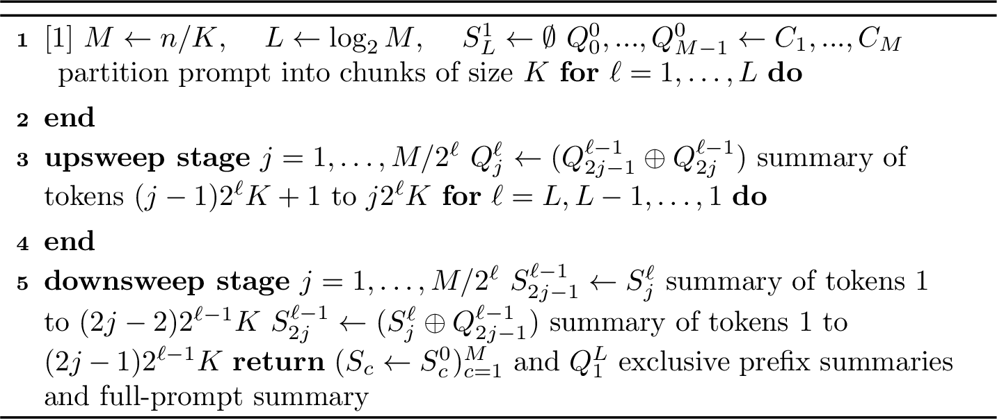
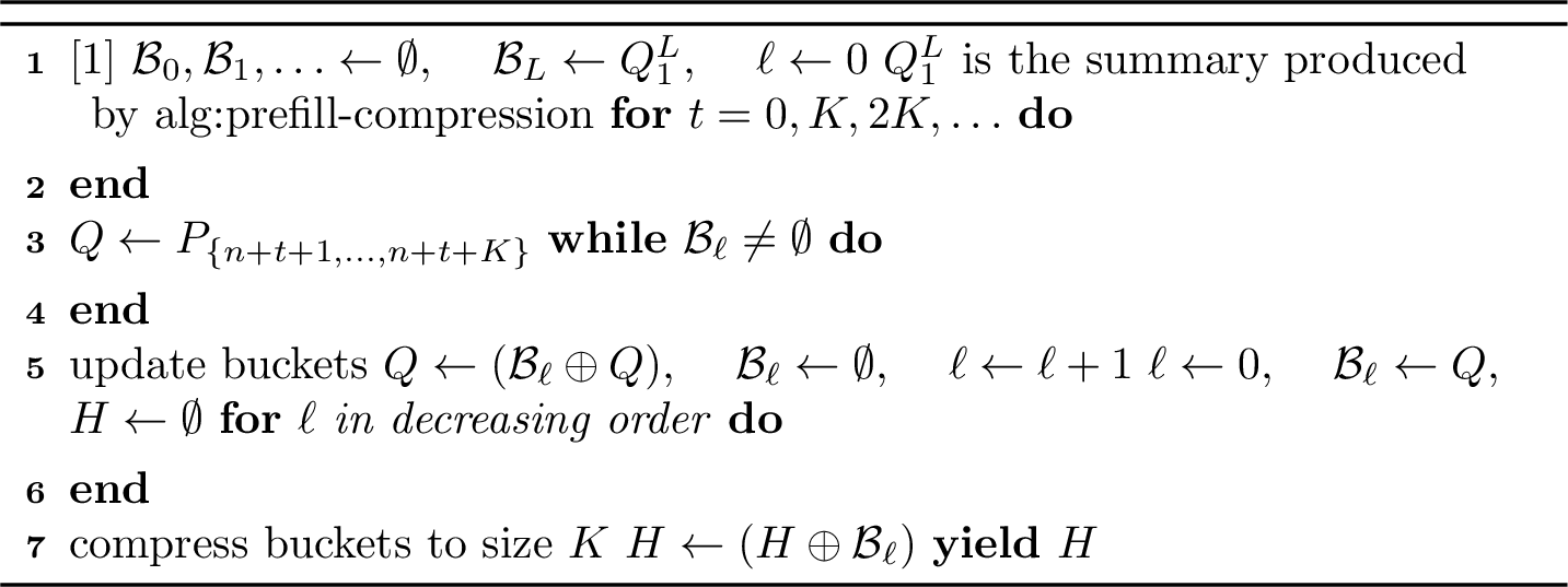
In causally masked prefill, token \(t\) may attend only to the prefix \(P_t \mathrel{\vcenter{:}}= P_{\{1,\dots,t\}}\), so compression must provide prefix summaries for each position \(t\). Since storing a separate summary for every prefix would defeat the purpose of compression, we summarize only at chunk boundaries. Specifically, we fix a chunk size \(K\), partition the stream into chunks \(I_1,I_2,\ldots\) of size \(K\), and maintain a \(K\)-atomic summary \(S_c\) of the prefix for each chunk \(c\). At position \(t \in I_c\), attention is then computed against \[\label{eq:summary} \hat{P}_t \mathrel{\vcenter{:}}= S_{c-1} \oplus P_{\{\min I_c,\dots,t\}},\tag{4}\] which keeps the local causal prefix exact and compresses only the long-range past. Hence, every attention computation uses at most \(2K\) atoms while respecting causal masking.
The summaries \(S_c\) are computed by recursively applying a randomized local reducer \(\mathop{\mathrm{\mathsf{REDUCE}}}: \mathcal{P}_{2K}(\mathcal{X}) \to \mathcal{P}_K(\mathcal{X})\). 2 implements this recursion as a parallel Blelloch scan over chunks, producing one \(K\)-atomic summary for each chunk prefix and one summary of the full prompt. 3 uses the same merge-reduce primitive online: starting from the prompt summary, it updates the compressed history during autoregressive decoding and emits a new \(K\)-atomic summary at each chunk boundary. Thus, both prefill and autoregressive decoding reduce to a small number of calls to \(\mathop{\mathrm{\mathsf{REDUCE}}}\) on inputs of size \(2K\). Consequently, if \(\mathop{\mathrm{\mathsf{REDUCE}}}\) can be implemented efficiently, the full compression scheme meets our efficiency desiderata, as the following proposition shows.
propositionproruntime 2 makes \(\mathop{\mathrm{\mathcal{O}}}(n/K)\) calls to \(\mathop{\mathrm{\mathsf{REDUCE}}}\), and uses parallel depth \(\mathop{\mathrm{\mathcal{O}}}(\log(n/K))\) and \(\mathop{\mathrm{\mathcal{O}}}(n)\) memory. Additionally, at time \(t\), 3 stores \(\mathop{\mathrm{\mathcal{O}}}(K \, \log(t/K))\) atoms, and makes \(\mathop{\mathrm{\mathcal{O}}}(\log(t/K)/K)\) calls to \(\mathop{\mathrm{\mathsf{REDUCE}}}\) amortized per token.
5.2 From local reducers to global risk guarantees↩︎
[alg:prefill-compression,alg:decoding-compression] lift any local compressor \(\mathop{\mathrm{\mathsf{REDUCE}}}:\kvmeasures[2K]\to\kvmeasures[K]\) to a global compression scheme for causally masked prefill and autoregressive decoding. It remains to identify conditions on \(\mathop{\mathrm{\mathsf{REDUCE}}}\) that yield global risk guarantees. We give such conditions below.
definitiondefdesigncriteria Fix \(K \ge 1\), a Hilbert space \(\mathcal{H}\), and \(\Phi: \mathcal{X}\to\mathcal{H}\). For \(P \in \kvmeasures\) and \(Q\in \kvmeasures[2K]\), define \[\textstyle \mu_P^\Phi \mathrel{\vcenter{:}}= \int_\mathcal{X}\Phi(k,v) \,\mathop{}\!\mathrm{d}P(k,v) \qquad \text{and} \qquad \Sigma_{P}^\Phi \mathrel{\vcenter{:}}= \int_\mathcal{X}(\Phi(k,v) - \mu_P^\Phi) \otimes (\Phi(k,v) - \mu_P^\Phi) \,\mathop{}\!\mathrm{d}P(k,v).\] We call \(\mathop{\mathrm{\mathsf{REDUCE}}}\) \((\Phi, r,\tau)\)-admissible for \(r,\tau \ge 0\) if, for all \(Q \in \kvmeasures[2K]\), \(\hat{Q} \mathrel{\vcenter{:}}= \mathop{\mathrm{\mathsf{REDUCE}}}(Q) \in \mathcal{P}_K(\mathop{\mathrm{supp}}(Q))\) almost surely and the following hold:
\(\mathop{\mathrm{\mathbb{E}}}[\hat{Q}] = Q\)
\(\mathop{\mathrm{\mathbb{E}}}\bigl[\|\int_{\mathcal{X}}\Psi \mathop{}\!\mathrm{d}(\hat{Q}-Q)\|_{\mathcal{G}}^2\bigr] \lesssim \frac{1}{K} \mathop{\mathrm{tr}}(\Sigma_Q^\Psi)\) for all Hilbert spaces \(\mathcal{G}\) and bounded \(\Psi: \mathcal{X}\to\mathcal{G}\)
\(\mathop{\mathrm{\mathbb{E}}}\bigl[\|\int_{\mathcal{X}}\Phi \mathop{}\!\mathrm{d}(\hat{Q}-Q)\|_\mathcal{H}^2\bigr] \lesssim \frac{1}{K} \bigl(\mathop{\mathrm{tail}}_r(\Sigma_Q^\Phi) + \tau \bigr)\)
Such reducers exist. We give concrete instantiations satisfying the conditions for any bounded \(\Phi\) in 10, together with a natural choice of \(\Phi\) and illustrative examples in which [asp:common-geometry] holds for this \(\Phi\). When \(\mathop{\mathrm{\mathsf{REDUCE}}}\) satisfies these conditions, we recover the minimax-optimal query-agnostic trace bound without further assumptions, and obtain the spectral refinement of query-aware compression under [asp:common-geometry].
theoremthmalgguarantee Let \(K \ge 1\) and \(\nu\in\mathcal{P}(\mathcal{Q})\), and suppose that \(\mathop{\mathrm{\mathsf{REDUCE}}}\) is \((\Phi,r,\tau)\)-admissible. Let \(\hat{P}_t \in \kvmeasures[2K]\) be as in 4 . Then, \(\mathop{\mathrm{\mathbb{E}}}\err*{P_t}{\nu}{\hat{P}_t} \lesssim \frac{\log(2+t/K)}{K} \mathop{\mathrm{tr}}(\Sigma_{P_t,\nu})\). If additionally [asp:common-geometry] holds for \(\nu\), \(P_t\), and \(\Phi\), then \(\mathop{\mathrm{\mathbb{E}}}\err*{P_t}{\nu}{\hat{P}_t} \lesssim \frac{\log(2+t/K)}{K} \, (\mathop{\mathrm{tail}}_r(\Sigma_{P_t,\nu}) + \tau)\).
6 Experiments↩︎
We conduct a focused long-context evaluation of the compression scheme from 5 on the “long” subset of LongBench-v2 [24], a multiple-choice benchmark with contexts ranging from \(128\mathrm{k}\) to \(2\mathrm{M}\) words. We evaluate Qwen3-32B [25]. As a baseline, we use attention over the entire available KV cache, following the official truncation protocol of [24] whenever the full context exceeds the model’s context window. We compare the baseline against our compression scheme from 5 and against ScissorHands [6], SnapKV [9], and StreamingLLM [8] from the literature, each applied independently to each attention head.
Since ScissorHands and SnapKV do not provide efficient parallel inference methods for compressed prefill, we let the literature baselines (including StreamingLLM) use the full KV cache during prefill and only compress during decoding. In contrast, our compression algorithm is used during both prefill and decoding, so that each head only ever attends to a small subset of the tokens seen by the full-attention baseline.
We evaluate our compression scheme for two local reducers. The first is random sampling from the context measure \(Q\), which attains the query-agnostic minimax-optimal rate. The second protects the leading \(r\) directions of \(\Sigma_Q^\Phi\) and clusters tokens in the protected coordinates. This reducer attains the spectral guarantee of [thm:alg-risk] under [asp:common-geometry]. We elaborate on the design of the clustering reducer and the choice of feature map \(\Phi\) in 10. 11 has additional implementation details.
1 reports accuracy with standard error for a compression rate of approximately \(95\%\) relative to full context window. Random sampling already provides a strong query-agnostic baseline, consistent with its minimax optimality. Admissible clustering improves accuracy at \(r=64\), and matches the uncompressed baseline at \(r=128\). Furthermore, all our local reducers are competitive with the literature baselines [6], [8], [9] despite using significantly fewer tokens during prefill. While we emphasize that standard errors overlap and further validation is warranted, these results suggest that the algorithmic design principles developed in 5 hold promise for practical long-context compression at substantial KV budget reductions, during both decoding and prefill.
| Method | Prefill budget | Decode budget | Protected rank | Accuracy (%) |
|---|---|---|---|---|
| Full KV | — | \(\best{37.04} \;(\pm 4.65\)) | ||
| Random (ours) | — | \(34.26 \;(\pm 4.57)\) | ||
| Balanced clustering (ours) | 64 | \(35.19 \;(\pm 4.60)\) | ||
| Balanced clustering (ours) | 128 | \(\best{37.04} \;(\pm 4.65)\) | ||
| ScissorHands [6] | — | \(35.19 \;(\pm 4.60)\) | ||
| SnapKV [9] | — | \(34.26 \;(\pm 4.57)\) | ||
| StreamingLLM [8] | — | \(32.41 \;(\pm 4.50)\) |
6pt
7 Conclusion↩︎
We posit KV compression as sparse balancing of a finite probability measure in Hilbert space, and characterize its minimax risk in terms of how a cache interacts with future queries through softmax attention. This yields tight rates under natural assumptions and identifies what compressed summaries must preserve. The same characterization reveals design principles for causal compression during prefill and autoregressive decoding, separating universal guarantees from structure-exploiting refinements. Together, our results provide a principled path toward practical KV cache compression with theoretical guarantees.
Funded by the European Union. This work has received funding from the European High Performance Computing Joint Undertaking (JU) and from the German Federal Ministry of Research, Technology and Space (BMFTR), the Ministry of Culture and Science of North
Rhine-Westphalia (MKW NRW) and the Hessian Ministry of Science and Research, Arts and Culture (HMWK) under grant agreement No 101250682. LH was supported by the RWTH Research Ambassador Scholarship during his research stay at Stanford
University. CAA is supported by a Schmidt Science Fellowship. Computations were performed with computing resources granted by RWTH Aachen University under project thes2228.
Appendix Contents↩︎
8 Sparse barycenter balancing in Hilbert space↩︎
This appendix records an upper bound for the abstract balancing problem in [prb:barycenter-sparsification].
Theorem 1. Let \(\mathcal{H}\) be a real Hilbert space, and let \[\textstyle \mu = \sum_{i=1}^n p_i \,\delta_{x_i} \in \mathcal{P}_n(\mathcal{H})\] have mean zero and covariance operator \[\textstyle \Sigma\mathrel{\vcenter{:}}= \sum_{i=1}^n p_i\, x_i \otimes x_i.\] Let \(U \subseteq \mathcal{H}\) be a finite-dimensional subspace. Let \(d \mathrel{\vcenter{:}}= \dim U\), and let \(\Pi_U: \mathcal{H}\to \mathcal{H}\) be the orthogonal projector onto \(U\). Then, for every \(m \in \mathbb{N}\), there exists \(\hat{\mu} \in \mathcal{P}_{m + 2d + 2}(\mathop{\mathrm{supp}}(\mu))\) with \[\int_\mathcal{H}x\, d\hat{\mu} \in U^\perp \qquad\text{and}\qquad \left\|\int_\mathcal{H}x\, d\hat{\mu}\right\|_\mathcal{H}^2 \le \frac{20}{9m}\mathop{\mathrm{tr}}\bigl((I - \Pi_U) \Sigma\bigr).\]
Proof. Deferred to 8.3. ◻
While 1 only claims existence, we give a constructive proof with concrete algorithms. We later invoke this construction when we design KV compression algorithms in 10.
For our construction, we reduce sparsifying a finitely supported measure \(\mu = \sum_{i=1}^n p_i \,\delta_{x_i} \in \mathcal{P}_n(\mathcal{H})\) to a constrained rounding problem: Given a vector \((p_1, ..., p_n) \in [0,1]^n\), find a (random) rounded vector \((\hat{p}_1, ..., \hat{p}_n) \in [0,1]^n\) with at most \(m+2d+2\) fractional entries preserving the mass of \(p\) while satisfying linear constraints. As we show, mass preservation is sufficient to construct a sparse measure supported on at most \(m+2d+2\) points from such a constrained rounding procedure, and linear constraints are used to encode exact preservation of the barycenter in the subspace \(U\).
In 8.1, we first describe a general algorithm for constrained rounding with mass preservation. 8.2 then specializes this algorithm to sparsification of measures with a protected subspace, and 8.3 proves 1 from this.
8.1 Finite-dimensional constrained rounding↩︎
We first isolate a finite-dimensional constrained rounding procedure. Starting from a fractional weight vector, the goal is to round most coordinates while preserving mass and satisfying linear constraints. Such a procedure can be obtained as a straightforward application of the sub-isotropic rounding walk of [26]. Given a current point \(x\in[0,1]^n\), an alive set \(A\subseteq[n]\), and linear constraints, we write \[x^+ = \mathrm{\small SubIsoWalk}\!\left( x,A \;\middle|\; \sum_{s=1}^n z_s=m,\; \sum_{s=1}^n z_sc_s=0 \right)\] for the stopped phase of Bansal’s walk, restricted to the coordinates in \(A\), that returns a random point \(x^+\in[0,1]^n\) satisfying the constraints \[\sum_{s=1}^n x^+_s=m, \qquad \sum_{s=1}^n x^+_sc_s=0,\] and \(x^+_s=x_s\) for all \(s \not\in A\), such that at least one coordinate in \(A\) reaches \(0\) or \(1\). 4 simply applies this procedure iteratively until only \(2d+2\) fractional coordinates remain, which yields the following guarantees on the output.

Lemma 1. Fix \(n,d,m \in \mathbb{N}\). Let \(z \in [0,1]^n\) and \(c_1, ..., c_n \in \mathbb{R}^d\). Assume that \(\sum_{s=1}^n z_s \, c_s = 0\) and \(m \mathrel{\vcenter{:}}= \sum_{s=1}^n z_s \in \mathbb{N}\). Let \(Z \mathrel{\vcenter{:}}= \mathrm{\small ConstrainedPartialRound}(z, \, c_1, ..., c_n)\) be the random output of 4. Then, the following hold:
\(\sum_{s=1}^n Z_s = m\) almost surely
\(\sum_{s=1}^n Z_s \, c_s = 0\) almost surely
\(|\{s \in [n] \mid 0 < Z_s < 1\}| \le 2d+2\) almost surely
\(\mathop{\mathrm{\mathbb{E}}}[Z] = z\)
for every \(a \in \mathbb{R}^n\), \[\mathop{\mathrm{\mathbb{E}}}\!\left[\Bigl(\sum_{s=1}^n (Z_s - z_s) \, a \Bigr)^2\right] \le \frac{20}{9}\sum_{s=1}^n a_s^2 z_s (1-z_s).\]
Proof. For \(x\in[0,1]^n\), let \[A(x)\mathrel{\vcenter{:}}= \{s\in[n] : x_s\in(0,1)\}\] be the alive set. The algorithm runs the sub-isotropic rounding walk of [26] with the following deterministic schedule of active constraints. As long as \(|A(x)|>2d+2\), we keep the constraints \[\sum_{s=1}^n x_s=m \qquad \text{and} \qquad \sum_{s=1}^n x_sc_s=0\] active on the alive coordinates. Once \(|A(x)|\le 2d+2\), the algorithm stops.
We first check that the active constraints satisfy the rank condition required by [26]. Restricted to the alive coordinates, the active system has at most \(d+1\) scalar constraints. Whenever the loop is entered, \(|A(x)|>2d+2\), and therefore \[d+1 \le \frac{|A(x)|}{2}.\] Thus the slack hypothesis in [26] holds with parameter \(\delta=1/2\).
Let \((z^{(k)})_{k\ge 0}\) denote the elementary iterates of the resulting walk, and let \((\mathcal{F}_k)_{k\ge 0}\) be its natural filtration. Let \(T\) be the terminal time of the full walk and write \[X \mathrel{\vcenter{:}}= z^{(T)} \in \{0,1\}^n\] for the final integral vector. By the martingale property of Bansal’s walk, \(\mathop{\mathrm{\mathbb{E}}}[X]=z\). Let \[\tau \mathrel{\vcenter{:}}= \inf\left\{ k\ge 0 : \bigl|A(z^{(k)})\bigr|\le 2d+2 \right\}.\] Then, \(Z\mathrel{\vcenter{:}}= z^{(\tau)}\).
Before time \(\tau\), every increment lies in the nullspace of the active constraints. Hence, the identities \[\sum_{s=1}^n z_s^{(k)}=m \qquad\text{and}\qquad \sum_{s=1}^n z_s^{(k)}c_s=0\] are preserved pathwise for all \(k\le\tau\). Since they hold at initialization, they hold for \(Z\), which proves \[\sum_{s=1}^n Z_s=m, \qquad \sum_{s=1}^n Z_sc_s=0 .\] The definition of \(\tau\) gives \[\bigl|\{s\in[n] \mid 0<Z_s<1\}\bigr|\le 2d+2 .\]
It remains to prove unbiasedness and the scalar second-moment bound. For \(k\ge 1\), set \[\Delta^{(k)}\mathrel{\vcenter{:}}= z^{(k)}-z^{(k-1)},\] and put \(\Delta^{(k)}\mathrel{\vcenter{:}}= 0\) for \(k>T\). In the notation of [26], conditional on \(\mathcal{F}_{k-1}\), the increment on the alive coordinates is of the form \(\gamma_k U_k^{1/2}r_k\), where \(r_k\) is a random sign vector and \(U_k\) is positive semidefinite with range contained in the nullspace of the active constraints. Embedding the conditional covariance into \(\mathbb{R}^n\) and padding zeros outside the alive coordinates gives a matrix \(\widetilde{U}_k\) such that \[\mathop{\mathrm{\mathbb{E}}}[\Delta^{(k)}\mid\mathcal{F}_{k-1}]=0, \qquad \mathop{\mathrm{\mathbb{E}}}\!\left[ \Delta^{(k)}(\Delta^{(k)})^\top \mid\mathcal{F}_{k-1} \right] = \widetilde{U}_k .\] Moreover, the sub-isotropic covariance estimate in the same construction gives, for \(\delta=1/2\), \[\widetilde{U}_k \preceq \frac{20}{9}\operatorname{diag}(\widetilde{U}_k).\]
Fix \(a\in\mathbb{R}^n\). Since \((\langle a,z^{(k)}\rangle)_{k\ge 0}\) is a martingale, its increments are orthogonal in \(L_2\). Hence, \[\mathop{\mathrm{\mathbb{E}}}\!\left[ \bigl\langle a,X-z\bigr\rangle^2 \right] = \sum_{k\ge 1} \mathop{\mathrm{\mathbb{E}}}\!\left[ \bigl\langle a,\Delta^{(k)}\bigr\rangle^2 \right].\] Using the conditional covariance estimate, \[\begin{align} \mathop{\mathrm{\mathbb{E}}}\!\left[ \bigl\langle a,\Delta^{(k)}\bigr\rangle^2 \mid \mathcal{F}_{k-1} \right] &= a^\top \widetilde{U}_k a \\ &\le \frac{20}{9} \sum_{s=1}^n a_s^2(\widetilde{U}_k)_{ss} \\ &= \frac{20}{9} \sum_{s=1}^n a_s^2 \mathop{\mathrm{\mathbb{E}}}\!\left[ (\Delta_s^{(k)})^2 \mid \mathcal{F}_{k-1} \right]. \end{align}\] Summing over \(k\) and taking expectations yields \[\mathop{\mathrm{\mathbb{E}}}\!\left[ \bigl\langle a,X-z\bigr\rangle^2 \right] \le \frac{20}{9} \sum_{s=1}^n a_s^2 \sum_{k\ge 1}\mathop{\mathrm{\mathbb{E}}}\!\left[(\Delta_s^{(k)})^2\right].\] For each coordinate \(s\), the process \((z_s^{(k)})_{k\ge0}\) is a bounded martingale with terminal value \(X_s\in\{0,1\}\). Its increments are orthogonal in \(L_2\), and therefore \[\sum_{k\ge 1}\mathop{\mathrm{\mathbb{E}}}\!\left[(\Delta_s^{(k)})^2\right] = \mathop{\mathrm{\mathbb{E}}}\!\left[(X_s-z_s)^2\right] = z_s(1-z_s),\] where we used \(X_s^2=X_s\) and \(\mathop{\mathrm{\mathbb{E}}}[X_s]=z_s\). Consequently, \[\mathop{\mathrm{\mathbb{E}}}\!\left[ \bigl\langle a,X-z\bigr\rangle^2 \right] \le \frac{20}{9} \sum_{s=1}^n a_s^2 z_s(1-z_s).\]
Finally, the stopped process \((z^{(k\wedge T)})_{k\ge0}\) is a bounded martingale and \(\tau\le T\) almost surely. Hence, optional stopping gives \[Z_s = z_s^{(\tau)} = \mathop{\mathrm{\mathbb{E}}}[X_s\mid\mathcal{F}_\tau]\] for every \(s\in[n]\). Taking expectations gives \(\mathop{\mathrm{\mathbb{E}}}[Z]=z\). Moreover, \[\bigl\langle a,Z-z\bigr\rangle = \mathop{\mathrm{\mathbb{E}}}\!\left[ \bigl\langle a,X-z\bigr\rangle \mid\mathcal{F}_\tau \right],\] and conditional Jensen yields \[\mathop{\mathrm{\mathbb{E}}}\!\left[ \bigl\langle a,Z-z\bigr\rangle^2 \right] \le \mathop{\mathrm{\mathbb{E}}}\!\left[ \bigl\langle a,X-z\bigr\rangle^2 \right] \le \frac{20}{9} \sum_{s=1}^n a_s^2 z_s(1-z_s).\] That proves the claim. ◻
8.2 Protected Hilbert rounding↩︎
We now apply the constrained rounding procedure to finitely supported measures on a Hilbert space. The linear constraints are chosen to preserve the barycenter in a protected subspace, and mass preservation forces small support.

Fix a Hilbert space \(\mathcal{H}\), a finite-dimensional subspace \(U\subseteq\mathcal{H}\) with \(d\mathrel{\vcenter{:}}=\dim(U)\), and some \(m\ge1\). Let \(\mu = \sum_{j=1}^S p_j \, \delta_{x_j} \in \mathcal{P}_{\mathrm{fin}}(\mathcal{H})\) and let \[\textstyle \hat{\mu} \mathrel{\vcenter{:}}= \mathrm{\small ProtectedSparsify}(\mu,U,m) = \sum_{j=1}^S \hat{p}_j \, \delta_{x_j}\] be the random output of 5. Write \[\textstyle \bar x\mathrel{\vcenter{:}}= \int_\mathcal{H}x \mathop{}\!\mathrm{d}\mu, \qquad \Sigma \mathrel{\vcenter{:}}= \int_\mathcal{H}(x-\bar x)\otimes(x-\bar x) \mathop{}\!\mathrm{d}\mu, \qquad \eta \mathrel{\vcenter{:}}= \int_\mathcal{H}x \mathop{}\!\mathrm{d}(\hat{\mu} - \mu).\] Then, the following hold:
\(\hat{\mu}\in\mathcal{P}_{m+2d+2}(\mathop{\mathrm{supp}}(\mu))\) almost surely
\(\int_\mathcal{H}x \mathop{}\!\mathrm{d}(\hat{\mu} - \mu) \in U^\perp\) almost surely
\(\mathop{\mathrm{\mathbb{E}}}[\hat{\mu}] = \mu\)
\(\mathop{\mathrm{\mathbb{E}}}[\eta \otimes \eta] \preceq \frac{20}{9m}(I-\Pi_U)\Sigma(I-\Pi_U)\)
Additionally, for every Hilbert space \(\mathcal{G}\) and every \(y_1,\ldots,y_S\in\mathcal{G}\), writing \[\textstyle \bar y\mathrel{\vcenter{:}}= \sum_{j=1}^S p_jy_j, \qquad \Sigma_y\mathrel{\vcenter{:}}= \sum_{j=1}^S p_j(y_j-\bar y)\otimes(y_j-\bar y),\] one has \[\mathop{\mathrm{\mathbb{E}}}\Bigl\| \sum_{j=1}^S(\hat{p}_j-p_j)y_j \Bigr\|_{\mathcal{G}}^2 \le \frac{20}{9m}\mathop{\mathrm{tr}}(\Sigma_y).\]
Proof. Use the notation of 5. We verify the four guarantees in the order suggested by the construction: first that the finite-dimensional rounding lemma applies, then support preservation and unbiasedness, then exact cancellation on \(U\), and finally the operator second-moment bound.
The splitting step gives \[\sum_{s=1}^N\alpha_s\delta_{y_s}=\mu, \qquad 0<\alpha_s\le \frac{1}{m} .\] Hence \(z_s=m\alpha_s\in[0,1]\) and \(\sum_s z_s=m\). Since \[\sum_{s=1}^N\alpha_s\xi_s = \int_\mathcal{H}(x-\bar x) \mathop{}\!\mathrm{d}\mu = 0,\] the protected coordinates satisfy \[\sum_{s=1}^N z_sc_s=0.\] Thus, \(\mathrm{\small ConstrainedPartialRound}\) applies. By 1, it returns \(Z\in[0,1]^N\) with \[\sum_{s=1}^N Z_s=m, \qquad \sum_{s=1}^N Z_sc_s=0, \qquad \mathop{\mathrm{\mathbb{E}}}[Z]=z,\] at most \(2d+2\) fractional coordinates, and, for every \(a\in\mathbb{R}^N\), \[\mathop{\mathrm{\mathbb{E}}}\!\left[ \left(\sum_{s=1}^N (Z_s-z_s)a_s\right)^2 \right] \le \frac{20}{9} \sum_{s=1}^N z_s(1-z_s)a_s^2 .\]
The non-fractional positive coordinates of \(Z\) are equal to \(1\), and their count is at most \(\sum_s Z_s=m\). Together with the at most \(2d+2\) fractional coordinates, this shows that at most \(m+2d+2\) split copies receive positive mass. After reassembling split copies, the same bound holds for the number of original atoms with \(\hat{p}_j>0\). Hence, \[\hat{\mu}\in\mathcal{P}_{m+2d+2}(\mathop{\mathrm{supp}}(\mu))\] almost surely.
Moreover, for each \(j\), \[\mathop{\mathrm{\mathbb{E}}}[\hat{p}_j] = \frac{1}{m}\sum_{s:\,\iota_s=j}\mathop{\mathrm{\mathbb{E}}}[Z_s] = \frac{1}{m}\sum_{s:\,\iota_s=j}z_s = \sum_{s:\,\iota_s=j}\alpha_s = p_j.\] Therefore, \[\mathop{\mathrm{\mathbb{E}}}[\hat{\mu}] = \sum_{j=1}^S \mathop{\mathrm{\mathbb{E}}}[\hat{p}_j]\delta_{x_j} = \sum_{j=1}^S p_j\delta_{x_j} = \mu.\]
By the reassembly definition of \(\hat{p}_j\), \[\eta = \sum_{j=1}^S(\hat{p}_j-p_j)x_j = \frac{1}{m}\sum_{s=1}^N (Z_s-z_s)y_s .\] Since \(\sum_s Z_s=\sum_s z_s=m\), the constant component \(\bar x\) cancels, and hence \[\eta = \frac{1}{m}\sum_{s=1}^N (Z_s-z_s)\xi_s.\] Moreover, \(\sum_s(Z_s-z_s)c_s=0\), and therefore \[\langle \eta,u_\ell\rangle = \frac{1}{m}\sum_{s=1}^N (Z_s-z_s)\langle \xi_s,u_\ell\rangle = 0 \qquad (\ell=1,\ldots,d).\] Thus \(\eta\in U^\perp\), and consequently \[\eta = \frac{1}{m}\sum_{s=1}^N (Z_s-z_s)(I-\Pi_U)\xi_s.\]
Fix \(h\in\mathcal{H}\), and apply the scalar second-moment bound with \(a_s=\langle h,(I-\Pi_U)\xi_s\rangle\). Since \(z_s=m\alpha_s\), \[\begin{align} \mathop{\mathrm{\mathbb{E}}}\langle h,\eta\rangle^2 &\le \frac{20}{9m^2} \sum_{s=1}^N z_s(1-z_s) \langle h,(I-\Pi_U)\xi_s\rangle^2 \\ &\le \frac{20}{9m} \sum_{s=1}^N \alpha_s \langle h,(I-\Pi_U)\xi_s\rangle^2 \\ &= \frac{20}{9m} \left\langle h,(I-\Pi_U)\Sigma_\mu(I-\Pi_U)h \right\rangle . \end{align}\] Since \(h\in\mathcal{H}\) was arbitrary, the operator inequality follows.
It remains to prove the auxiliary variance bound. Since \(\sum_j(\hat{p}_j-p_j)=0\), \[\sum_{j=1}^S(\hat{p}_j-p_j)y_j = \sum_{j=1}^S(\hat{p}_j-p_j)(y_j-\bar y).\] Using the split copies, \[\sum_{j=1}^S(\hat{p}_j-p_j)(y_j-\bar y) = \frac{1}{m} \sum_{s=1}^N (Z_s-z_s)(y_{\iota_s}-\bar y).\] Fix \(g\in\mathcal{G}\) and apply the scalar second-moment bound with \[a_s = \langle g,y_{\iota_s}-\bar y\rangle_{\mathcal{G}}.\] Then \[\mathop{\mathrm{\mathbb{E}}}\left[ \left\langle g, \sum_{j=1}^S(\hat{p}_j-p_j)y_j \right\rangle^2 \right] \le \frac{20}{9m^2} \sum_{s=1}^N z_s(1-z_s) \langle g,y_{\iota_s}-\bar y\rangle^2.\] Since \(z_s=m\alpha_s\le1\), \[z_s(1-z_s)\le m\alpha_s.\] Therefore, \[\mathop{\mathrm{\mathbb{E}}}\left\langle g, \sum_{j=1}^S(\hat{p}_j-p_j)y_j \right\rangle^2 \le \frac{20}{9m} \sum_{s=1}^N \alpha_s \langle g,y_{\iota_s}-\bar y\rangle^2.\] Reassembling the split copies gives \[\sum_{s=1}^N \alpha_s (y_{\iota_s}-\bar y)\otimes(y_{\iota_s}-\bar y) = \Sigma_y.\] Thus \[\mathop{\mathrm{\mathbb{E}}}\left\langle g, \sum_{j=1}^S(\hat{p}_j-p_j)y_j \right\rangle^2 \le \frac{20}{9m} \langle g,\Sigma_y g\rangle.\] Taking traces yields the claim. ◻
8.3 Proof of 1↩︎
1 now follows by running ProtectedSparsify on the measure \(\mu\) and subspace \(U\), and taking one random realization on which the desired bound holds.
Proof. Apply [pro:protected-sparsification] to \((\mu,U,m)\), and let \(\hat{\mu}\) denote the random output. Since \(\mu\) is centered, \[\eta \mathrel{\vcenter{:}}= \int_\mathcal{H}x \mathop{}\!\mathrm{d}\hat{\mu} = \int_\mathcal{H}x \mathop{}\!\mathrm{d}(\hat{\mu} - \mu).\] Hence, [pro:protected-sparsification] gives a random \(\hat{\mu}\) such that
\(\hat{\mu}\in\mathcal{P}_{m+2d+2}(\mathop{\mathrm{supp}}(\mu))\) almost surely;
\(\int_\mathcal{H}x \mathop{}\!\mathrm{d}\hat{\mu} \in U^\perp\) almost surely; and
\(\mathop{\mathrm{\mathbb{E}}}[\eta \otimes \eta] \preceq \frac{20}{9m}(I-\Pi_U)\Sigma(I-\Pi_U)\).
Moreover, taking traces in [itm:sparse-hilbert-approximation:3] gives \[\mathop{\mathrm{\mathbb{E}}}\left\|\int_\mathcal{H}x \mathop{}\!\mathrm{d}\hat{\mu}\right\|_\mathcal{H}^2 = \mathop{\mathrm{\mathbb{E}}}\|\eta\|_\mathcal{H}^2 \le \frac{20}{9m} \mathop{\mathrm{tr}}\bigl((I-\Pi_U)\Sigma(I-\Pi_U)\bigr) = \frac{20}{9m} \mathop{\mathrm{tr}}\bigl((I-\Pi_U)\Sigma\bigr).\] Therefore some realization of \(\hat{\mu}\) satisfies the same bound. ◻
9 Minimax rates↩︎
This appendix proves our minimax rates for KV compression in the query-aware and query-agnostic settings. 9.1 proves upper bounds and 9.2 proves the matching lower bounds.
9.0.0.1 Notation.
We briefly recall the relevant notation from the main text. Given a context measure \(P \in \kvmeasures\), we write softmax attention as \[\att*{q}{P} = \int_{\mathcal{X}} a_P(q,k)\, v \, \mathop{}\!\mathrm{d}P(k,v), \qquad a_k(q \mid P) = \frac{\kappa(q,k)}{\int_{\mathcal{X}} \kappa(q,k') \, \mathop{}\!\mathrm{d}P(k',v')}\] and study the mean squared error of compressed context measures \(\hat{P} \in \kvmeasures[K]\) \[\err*{P}{\nu}{\hat{P}} = \mathop{\mathrm{\mathbb{E}}}_{q \sim \nu}\!\left\|\att*{q}{P} - \att*{q}{\hat{P}}\right\|_2^2\] under a fixed query distribution \(\nu \in \mathcal{P}(\mathcal{Q})\). The response profile of a key–value pair \((k,v) \in \mathcal{X}\) under \(P\) is \[\Gamma_P(k,v) : \mathcal{Q}\to \mathbb{R}^{d_v}\oplus\mathbb{R}, \qquad q \mapsto \Bigl( a_k(q \mid P)\bigl(v-\att{q}{P}\bigr), \; V\bigl(a_k(q \mid P)-1\bigr) \Bigr),\] with the corresponding covariance operator \[\Sigma_{P,\nu} = \int_\mathcal{X}\Gamma_P(k,v) \otimes \Gamma_P(k,v) \,\mathop{}\!\mathrm{d}P(k,v),\] where \(\Gamma_P(k,v) \otimes \Gamma_P(k,v)\) is understood as the rank-one operator \[h \mapsto \dotp{\Gamma_P(k,v)}{h}_{\mathcal{H}_\nu} \cdot \Gamma_P(k,v)\] and \(\mathcal{H}_\nu = L_2(\nu, \mathbb{R}^{d_v} \oplus \mathbb{R})\).
9.1 Upper bounds↩︎
We derive upper bounds on the minimax compression risk in the query-aware and query-agnostic settings from a shared Hilbert space representation. For fixed \((P,\nu)\), the response profile map \(\Gamma_P\) sends each token \((k,v)\) to an element of the Hilbert space \(\mathcal{H}_\nu\), and thereby pushes the context measure \(P\) forward to a finitely supported probability measure on \(\mathcal{H}_\nu\). This measure is centered and has covariance \(\Sigma_{P,\nu}\), and the attention error of a compressed context is controlled by the squared norm of the corresponding barycenter in \(\mathcal{H}_\nu\). The query-aware and query-agnostic regimes differ only in how this barycenter is approximated: in the aware regime, we may choose a sparse approximation after seeing \(\nu\), whereas in the agnostic regime we must rely on a query-independent approximation. Both regimes permit upper bounds on the sparse barycenter approximation problem, which we then translate back to bounds on the KV compression problem.
9.1.1 Reduction to barycenter sparsification↩︎
Recall the surrogate error definition \[\widetilde{\mathcal{E}}_{\mu}(\hat{\mu}) = \left\|\int_{\mathcal{H}} g \,\mathop{}\!\mathrm{d}\hat{\mu}(g)\right\|_{\mathcal{H}}^2\] between measures \(\mu\) and \(\hat{\mu}\) on a Hilbert space \(\mathcal{H}_\nu\). Our goal is to derive upper bounds on the compression error \(\mathcal{E}_{P,\nu}(\hat{P})\) from upper bounds on \(\widetilde{\mathcal{E}}(\hat{\mu})\) for the pushforward \(\mu_{P,\nu} = P \circ \Gamma_P^{-1}\) by pulling back a sparse approximation \(\hat{\mu} \in \mathcal{P}_K(\mathop{\mathrm{supp}}(\mu_{P,\nu}))\) of \(\mu_{P,\nu}\) to a sparse approximation \(\hat{P} \in \kvmeasures[K]\) of \(P\). 2 first shows that upper bounds on \(\widetilde{\mathcal{E}}\) indeed survive this pullback, and [pro:reduction] packages the full reduction principle.
Lemma 2. Let \(P \in \kvmeasures\), \(\nu \in \mathcal{P}(\mathcal{Q})\), and let \(\hat{P} \in \mathcal{P}(\mathop{\mathrm{supp}}(P))\). Then, \[\err*{P}{\nu}{\hat{P}} \le 16 \left\| \int_{\mathcal{X}} \Gamma_P(k,v)\,\mathop{}\!\mathrm{d}\hat{P}(k,v) \right\|_{\mathcal{H}_\nu}^2.\]
Proof of 2. Fix \(q \in \mathop{\mathrm{supp}}(\nu)\), and abbreviate \[m_P(q) \mathrel{\vcenter{:}}= \int_{\mathcal{X}} \kappa(q,k)\,\mathop{}\!\mathrm{d}P(k,v), \qquad m_{\hat{P}}(q) \mathrel{\vcenter{:}}= \int_{\mathcal{X}} \kappa(q,k)\,\mathop{}\!\mathrm{d}\hat{P}(k,v).\] Define \[U(q) \mathrel{\vcenter{:}}= \int_{\mathcal{X}} a_k(q \mid P)\bigl(v-\att*{q}{P}\bigr)\,\mathop{}\!\mathrm{d}\hat{P}(k,v),\] and \[t(q) \mathrel{\vcenter{:}}= \int_{\mathcal{X}} \bigl(a_k(q \mid P)-1\bigr)\,\mathop{}\!\mathrm{d}\hat{P}(k,v).\] Since \(\hat{P}\) is a probability measure, \[1+t(q) = \int_{\mathcal{X}} a_k(q \mid P)\,\mathop{}\!\mathrm{d}\hat{P}(k,v) = \frac{m_{\hat{P}}(q)}{m_P(q)} \ge 0.\] Also, \[\begin{align} \att*{q}{\hat{P}} &= \frac{\int_{\mathcal{X}} \kappa(q,k) v\,\mathop{}\!\mathrm{d}\hat{P}(k,v)}{m_{\hat{P}}(q)} = \frac{\int_{\mathcal{X}} a_k(q \mid P) v\,\mathop{}\!\mathrm{d}\hat{P}(k,v)}{1+t(q)} \\ &= \frac{\att*{q}{P} + U(q) + t(q)\att*{q}{P}}{1+t(q)} = \att*{q}{P} + \frac{U(q)}{1+t(q)}. \end{align}\] Hence \[\att*{q}{\hat{P}} - \att*{q}{P} = \frac{U(q)}{1+t(q)}.\] On the other hand, \[\int_{\mathcal{X}} \Gamma_P(k,v)(q)\,\mathop{}\!\mathrm{d}\hat{P}(k,v) = \bigl(U(q),V t(q)\bigr) \in \mathbb{R}^{d_v+1}.\]
Since both \(\att*{q}{P}\) and \(\att*{q}{\hat{P}}\) are convex combinations of values, we have \[\left\|\att*{q}{\hat{P}}-\att*{q}{P}\right\|_2 \le 2V.\] If \(1+t(q)\ge \frac{1}{2}\), then \[\left\|\att*{q}{\hat{P}}-\att*{q}{P}\right\|_2^2 = \left\|\frac{U(q)}{1+t(q)}\right\|_2^2 \le 4\|U(q)\|_2^2.\] If \(1+t(q)<\frac{1}{2}\), then \(t(q)^2\ge \frac{1}{4}\), and therefore \[\left\|\att*{q}{\hat{P}}-\att*{q}{P}\right\|_2^2 \le 4V^2 \le 16V^2 t(q)^2.\] Thus, in all cases, \[\left\|\att*{q}{\hat{P}}-\att*{q}{P}\right\|_2^2 \le 16\bigl(\|U(q)\|_2^2 + V^2 t(q)^2\bigr) = 16\left\| \int_{\mathcal{X}} \Gamma_P(k,v)(q)\,\mathop{}\!\mathrm{d}\hat{P}(k,v) \right\|_{\mathbb{R}^{d_v} \oplus \mathbb{R}}^2.\] Averaging over \(q\sim \nu\) then yields the claim. ◻
Proof of [pro:reduction]. We first show that \(\mu_{P,\nu}\) is centered. For every \(q \in \mathcal{Q}\), \[\begin{align} &\phantom{=} \int_{\mathcal{X}} \Gamma_P(k,v)(q)\,\mathop{}\!\mathrm{d}P(k,v) \\ &= \left( \int_{\mathcal{X}} a_k(q \mid P)\bigl(v-\att*{q}{P}\bigr)\,\mathop{}\!\mathrm{d}P(k,v), \; V\left(\int_{\mathcal{X}} a_k(q \mid P)\,\mathop{}\!\mathrm{d}P(k,v)-1\right) \right) \\ &= (0,0), \end{align}\] since \[\int_{\mathcal{X}} a_k(q \mid P)\,\mathop{}\!\mathrm{d}P(k,v)=1 \qquad\text{and}\qquad \int_{\mathcal{X}} a_k(q \mid P)\,v\,\mathop{}\!\mathrm{d}P(k,v)=\att*{q}{P}.\] Thus, \(\int_{\mathcal{H}_\nu} g \mathop{}\!\mathrm{d}\mu_{P,\nu}(g) = 0\).
For the covariance identity, we have \[\begin{align} \int_{\mathcal{H}_\nu} g \otimes g \,\mathop{}\!\mathrm{d}\mu_{P,\nu}(g) = \int_{\mathcal{X}} \Gamma_P(k,v) \otimes \Gamma_P(k,v) \,\mathop{}\!\mathrm{d}P(k,v) = \Sigma_{P,\nu} \end{align}\] by the definition of \(\Sigma_{P,\nu}\).
Now, let \(\hat{\mu} \in \mathcal{P}_K(\mathop{\mathrm{supp}}(\mu_{P,\nu}))\). Write \[\hat{\mu} = \sum_{\ell=1}^m \beta_\ell \delta_{g_\ell}, \qquad m \le K,\] with \(g_\ell \in \mathop{\mathrm{supp}}(\mu_{P,\nu})\), \(\beta_\ell \ge 0\), and \(\sum_{\ell=1}^m \beta_\ell = 1\).
For each \(\ell \in [m]\), choose one atom \((\hat{k}_\ell,\hat{v}_\ell) \in \mathop{\mathrm{supp}}(P)\) such that \[\Gamma_P(\hat{k}_\ell,\hat{v}_\ell) = g_\ell.\] This is possible because \(g_\ell \in \mathop{\mathrm{supp}}(P \circ \Gamma_P^{-1})\). Define \[\hat{P} \mathrel{\vcenter{:}}= \sum_{\ell=1}^m \beta_\ell \delta_{(\hat{k}_\ell,\hat{v}_\ell)}.\] Then, \(\hat{P} \in \mathcal{P}_K(\mathop{\mathrm{supp}}(P))\) depends on \(\hat{\mu}\) but not on \(\nu\), and \[\int_{\mathcal{X}} \Gamma_P(k,v)\,\mathop{}\!\mathrm{d}\hat{P}(k,v) = \sum_{\ell=1}^m \beta_\ell \Gamma_P(\hat{k}_\ell,\hat{v}_\ell) = \sum_{\ell=1}^m \beta_\ell g_\ell = \int_{\mathcal{H}_\nu} g\,\mathop{}\!\mathrm{d}\hat{\mu}(g).\]
Therefore, by 2, \[\err*{P}{\nu}{\hat{P}} \le 16\left\| \int_{\mathcal{X}} \Gamma_P(k,v)\,\mathop{}\!\mathrm{d}\hat{P}(k,v) \right\|_{\mathcal{H}_\nu}^2 = 16\left\| \int_{\mathcal{H}_\nu} g\,\mathop{}\!\mathrm{d}\hat{\mu}(g) \right\|_{\mathcal{H}_\nu}^2.\] Since \(\hat{\mu} \in \mathcal{P}_K(\mathop{\mathrm{supp}}(\mu_{P,\nu}))\) was arbitrary, that proves the claim. ◻
9.1.2 Query-aware upper bound↩︎
In the query-aware regime, the compressor may depend on \(\nu\), and therefore on the geometry of \(\mathcal{H}_\nu\). After the reduction above, the problem is exactly to approximate the zero barycenter of the pushed-forward measure \(\mu_{P,\nu}\) by a \(K\)-atomic measure on \(\mathop{\mathrm{supp}}(\mu_{P,\nu})\). This is exactly the setting of [thm:sparse-hilbert-approximation-fixed-K], which provides a barycenter bound in terms of the spectral tail of its covariance, which here is \(\Sigma_{P,\nu}\). Pulling the resulting sparse measure back to \(\mathop{\mathrm{supp}}(P)\) then gives the desired compression bound for KV compression.
Proof. Choose \(r \mathrel{\vcenter{:}}= \lfloor K/3 \rfloor\) and \(M \mathrel{\vcenter{:}}= K - 2r - 2\). Further, choose \(U\) to be the span of the top \(r_\ast \mathrel{\vcenter{:}}= \min\{r,\mathop{\mathrm{rank}}(\Sigma)\}\) eigenvectors of \(\Sigma\). Then, \(\dim(U)=r_\ast\le r\). Invoking 1 with subspace \(U\) and support size parameter \(M\) yields \(\hat{\mu} \in \mathcal{P}(\mathop{\mathrm{supp}}(\mu))\) with \(\mathop{\mathrm{supp}}(\hat{\mu}) \le M + 2r + 2 \le K\) and \[\left\|\int_\mathcal{H}x\, d\hat{\mu}(x)\right\|_\mathcal{H}^2 \le \frac{20}{9M}\mathop{\mathrm{tr}}\bigl((I - \Pi_U) \Sigma\bigr) = \frac{20}{9M}\mathop{\mathrm{tail}}_r(\Sigma). \tag*{\qedhere}\] ◻
Proof. This is immediate from [pro:reduction] and [thm:sparse-hilbert-approximation-fixed-K]. ◻
9.1.3 Query-agnostic upper bound↩︎
In the query-agnostic regime, the compressor cannot adapt to \(\nu\), so the sparse approximation argument from the aware case does not apply. A natural query-independent alternative is the empirical measure of \(K\) i.i.d. samples from \(P\). Under the Hilbert embedding, this corresponds to averaging \(K\) independent copies of the centered random response profile \(G=\Gamma_P(X)\). The mean remains zero, and the mean squared norm of the empirical average is of order \(\mathop{\mathrm{tr}}(\Sigma_{P,\nu})/K\). Using 2 from the reduction, this yields the trace upper bound.
Lemma 3. Let \(\mathcal{H}\) be a real Hilbert space, and let \(\mu \in \mathcal{P}_\mathrm{fin}(\mathcal{H})\) be centered, with covariance operator \(\Sigma\). Let \(G_1,\dots,G_K \stackrel{\mathrm{iid}}{\sim} \mu\), and define \[\hat{\mu}_K \mathrel{\vcenter{:}}= \frac{1}{K} \sum_{i=1}^K \delta_{G_i}.\] Then, \[\mathop{\mathrm{\mathbb{E}}}\left[ \widetilde{\mathcal{E}}_\mu(\hat{\mu}_K) \right] = \frac{\mathop{\mathrm{tr}}(\Sigma)}{K}.\]
Proof. Since \(\mu\) is centered, the \(G_i\) are independent and mean zero. Hence \[\mathop{\mathrm{\mathbb{E}}}\left[ \widetilde{\mathcal{E}}_\mu(\hat{\mu}_K) \right] = \mathop{\mathrm{\mathbb{E}}}\left\| \frac{1}{K} \sum_{i=1}^K G_i \right\|_\mathcal{H}^2 = \frac{1}{K^2}\sum_{i=1}^K \mathop{\mathrm{\mathbb{E}}}\|G_i\|_\mathcal{H}^2 = \frac{\mathop{\mathrm{tr}}(\Sigma)}{K}.\] ◻
Proof. Let \(P \in \kvmeasures\) and \(\nu \in \mathcal{P}(\mathcal{Q})\). Let \(X_1,\dots,X_K\stackrel{\mathrm{iid}}{\sim}P\), set \[G_i=\Gamma_P(X_i), \qquad \hat{\mu}_K=\frac{1}{K}\sum_{i=1}^K\delta_{G_i}.\] By [pro:reduction], \(\hat{\mu}_K\) can be pulled back to the empirical context measure \[\hat{P}=\frac{1}{K}\sum_{i=1}^K\delta_{X_i}\] with \[\err*{P}{\nu}{\hat{P}} \lesssim \widetilde{\mathcal{E}}_{\mu_{P,\nu}}(\hat{\mu}_K).\] Taking expectations and applying 3 with \(\mu=\mu_{P,\nu}\) and \(\Sigma=\Sigma_{P,\nu}\) gives \[\mathop{\mathrm{\mathbb{E}}}[\err*{P}{\nu}{\hat{P}}] \lesssim \frac{\mathop{\mathrm{tr}}(\Sigma_{P,\nu})}{K}.\] The claim then follows because random sampling from \(P\) can be implemented by a randomized query-agnostic compressor. ◻
9.2 Lower bounds↩︎
We now provide lower bounds on the query-aware and query-agnostic minimax compression risk matching the upper bounds from 9.1. Both bounds are derived from a shared, explicit construction of an instance of a context \(P\) and a query distribution \(\nu\) that are realizable from actual keys, queries, and values under [asp:richness]. This instance is constructed so that any significant compression of the context incurs large error over the chosen query distribution. We then specialize this construction to the query-aware and query-agnostic regime by calibrating the error incurred under compression against the spectrum of \(\Sigma_{P,\nu}\), obtaining lower bounds that faithfully match their corresponding upper bounds throughout the entire claimed range of redundancy levels captured by \(\mathop{\mathrm{tr}}(\Sigma_{P,\nu})\) and \(\mathop{\mathrm{tail}}_{K/3}(\Sigma_{P,\nu})\), respectively.
Throughout this section, fix universal constants \[\textstyle \rho_0\mathrel{\vcenter{:}}= \frac{99}{100} \qquad \text{and} \qquad \gamma_0\mathrel{\vcenter{:}}= \frac{9}{10}.\]
9.2.1 Hard instance construction↩︎
We begin by constructing a pair \(P,\nu\) that is impossible to compress significantly without incurring large error. The main idea is to use keys that can be sharply distinguished from each other, and have them carry almost orthogonal values. We call such an instance a lookup instance because querying a key of the context sharply retrieves the associated value. 5 formalizes the properties of a lookup instance formally, and 4 shows that such instances can indeed be constructed from actual keys, queries, and values under [asp:richness]. In particular, [asp:richness] provides enough ambient dimension to choose well-separated keys and values from Hamming packings, and enough key/query norm budget to address the keys sharply through softmax attention.
Definition 5 (Lookup instance). Fix an even integer \(N \ge 2\) and let \[\textstyle P_N \mathrel{\vcenter{:}}= \frac{1}{N} \sum_{i=1}^N \delta_{(k_i,v_i)}, \qquad \nu_N \mathrel{\vcenter{:}}= \frac{1}{N} \sum_{i=1}^N \delta_{k_i}.\] We call the pair \((P_N,\nu_N)\) a lookup instance of size \(N\)* if*
\(k_i\in\mathcal{K}\cap \mathcal{Q}\), and \(v_i\in\mathcal{V}\) for all \(i\in[N]\);
\(\frac{1}{N} \sum_{i=1}^N v_i = 0;\)
\(\|v_i\|_2=\rho_0 V\) for all \(i\in[N]\);
\(\dotp{v_i}{v_j} \le \gamma_0\rho_0^2V^2\) for all \(i \neq j\);
\(\frac{1}{N} \sum_{j\neq i} a_{k_j}(k_i\mid P_N) \le N^{-3/2}\) for all \(i\in[N]\).
Lemma 4. Let \(K\ge 50\), set \(N\mathrel{\vcenter{:}}= 2K\), and suppose [asp:richness] holds. Then, there exists a lookup instance \(\bigl(P_N,\nu_N\bigr) \in \kvmeasures*[N] \times \mathcal{P}(\mathcal{Q})\) of size \(N\) such that
\(|\mathop{\mathrm{supp}}(\nu_N)| = |\mathop{\mathrm{supp}}(P_N)| = N\);
\(\dim \mathop{\mathrm{span}}\{v_1,\ldots,v_N\} \le K/6\); and
\(\|k\|_2 = 5d_k^{1/4}\sqrt{\log N}\) for all \(k \in \mathop{\mathrm{supp}}(\nu_N)\).
Proof. For \(r\ge 1\), set \[B_r \mathrel{\vcenter{:}}= \sum_{\ell=0}^{\lfloor r/20\rfloor}\binom{r}{\ell}.\] We first construct a Hamming packing. Greedily select words from \(x \in \{\pm1\}^r\). After selecting \(x\), delete the Hamming balls of radius \(\lfloor r/20\rfloor\) around \(x\) and around \(-x\). Each step deletes at most \(2B_r\) words, so the set \(\mathsf C_r\subseteq\{\pm1\}^r\) selected by the greedy procedure satisfies \[|\mathsf C_r| \ge \frac{2^r}{2B_r}.\] Denote by \(d_H\) the Hamming distance. If \(x,x'\in\mathsf C_r\) are distinct, then \[d_H(x,x')>\lfloor r/20\rfloor \qquad \text{and} \qquad d_H(x,-x')>\lfloor r/20\rfloor.\] Since \(\dotp{x}{x'}=r-2d_H(x,x')\), this implies \[|\dotp{x}{x'}| \le \gamma_0 r .\]
Using the entropy bound for Hamming balls, for \(r\ge 20\), \[B_r \le \exp\!\left( r\left[ -\frac{1}{20}\log\frac{1}{20} -\frac{19}{20}\log\frac{19}{20} \right] \right) \le \exp(0.2r).\] Hence, for \(r\ge 20\), \[\label{eq:lookup-instance-membership:code-size} |\mathsf C_r| \ge \frac{1}{2}\exp((\log 2-0.2)r).\tag{5}\] In particular, if \(r\ge 10\log K\), then \[\label{eq:lookup-instance-membership:code-size-large} |\mathsf C_r| \ge \frac{1}{2}K^{4.9} \ge 2K,\tag{6}\] where the last inequality uses \(K\ge 50\). Also, if \(r\ge 8\), then \[\label{eq:lookup-instance-membership:code-size-small} |\mathsf C_r|\ge 6r+5.\tag{7}\] Indeed, for \(8\le r<20\), this follows from \(B_r=1\) and \(2^{r-1}\ge 6r+5\). For \(r\ge20\), 5 gives \[|\mathsf C_r| \ge \frac{1}{2}\exp((\log 2-0.2)r) \ge 6r+5.\]
Let \(N\mathrel{\vcenter{:}}= 2K\). Choose distinct \(\xi_1,\ldots,\xi_N\in\mathsf C_{d_k}\), and define \[R_k\mathrel{\vcenter{:}}= 5d_k^{1/4}\sqrt{\log N}, \qquad \text{and} \qquad k_i\mathrel{\vcenter{:}}= R_k\frac{\xi_i}{\sqrt{d_k}}\] for \(i\in[N]\). Since \(d_k\ge 10\log K\), the code \(\mathsf C_{d_k}\) has at least \(2K=N\) words. Moreover, \[\|k_i\|_2=R_k = 5d_k^{1/4}\sqrt{\log N} \le 8d_k^{1/4}\sqrt{\log K},\] so \(k_i\in\mathcal{K}\cap\mathcal{Q}\) by [asp:richness].
Set \[r_v\mathrel{\vcenter{:}}= \min\{d_v,\lfloor K/6\rfloor\}.\] Then \(r_v\ge 8\), since \(d_v\ge 10\log K\) and \(K\ge 50\). The code \(\mathsf C_{r_v}\) has at least \(K\) words. If \(r_v=d_v\), this follows from 6 , because then \(r_v\ge 10\log K\). If \(r_v=\lfloor K/6\rfloor\), it follows from 7 , because then \(r_v\ge 8\) and \(6r_v+5\ge K\). Choose distinct \(\zeta_1,\ldots,\zeta_K\in\mathsf C_{r_v}\), and let \(E:\mathbb{R}^{r_v}\to\mathbb{R}^{d_v}\) be the canonical coordinate embedding. Define \[u_\ell\mathrel{\vcenter{:}}= E\frac{\zeta_\ell}{\sqrt{r_v}}, \qquad v_\ell\mathrel{\vcenter{:}}= \rho_0V u_\ell, \qquad v_{K+\ell}\mathrel{\vcenter{:}}= -\rho_0V u_\ell\] for \(\ell \in[K]\). Then, \(v_i\in\mathcal{V}=\mathsf{B}_{d_v}(V)\), \[\frac{1}{N}\sum_{i=1}^N v_i=0, \qquad \text{and} \qquad \|v_i\|_2=\rho_0V\] for all \(i\in[N]\). For \(i\neq j\), \[\dotp{v_i}{v_j} \le \gamma_0\rho_0^2V^2.\] Also, \[\dim\mathop{\mathrm{span}}\{v_1,\ldots,v_N\} \le \dim \mathop{\mathrm{im}}(E) \le r_v \le K/6.\]
Define \[P_N\mathrel{\vcenter{:}}= \frac{1}{N}\sum_{i=1}^N\delta_{(k_i,v_i)}, \qquad \text{and} \qquad \nu_N\mathrel{\vcenter{:}}= \frac{1}{N}\sum_{i=1}^N\delta_{k_i}.\] Since \(k_i \in \mathcal{K}\cap \mathcal{Q}\) and \(\|v_i\|_2 \le V\) for all \(i \in [N]\), \(P_N \in \kvmeasures*[N]\) and \(\nu_N \in \mathcal{P}(\mathcal{Q})\).
The keys \(k_i\) are distinct, so \[|\mathop{\mathrm{supp}}(P_N)|=|\mathop{\mathrm{supp}}(\nu_N)|=N.\]
It remains to verify sharpness. For \(i\neq j\), \[\frac{\dotp{k_i}{k_j}}{\sqrt{d_k}} \le 25\gamma_0\log N,\] while \[\frac{\|k_i\|_2^2}{\sqrt{d_k}} = 25\log N.\] Hence, for \(j\neq i\), \[a_{k_j}(k_i\mid P_N) = \frac{ N\exp(\dotp{k_i}{k_j}/\sqrt{d_k}) }{ \sum_{m=1}^N\exp(\dotp{k_i}{k_m}/\sqrt{d_k}) } \le N\exp(-25(1-\gamma_0)\log N) = N^{-3/2}.\] Therefore, \[\frac{1}{N}\sum_{j\neq i}a_{k_j}(k_i\mid P_N) \le N^{-3/2}\] for all \(i\in[N]\).
Thus, \((P_N,\nu_N)\) is a lookup instance of size \(N\), and it satisfies (i)–(iii). ◻
9.2.2 Approximating lookup instances requires almost the full context↩︎
We now show that lookup instances are hard to compress. Indeed, querying a key of such an instance retrieves the associated value almost perfectly, and the retrievable values are separated by a constant fraction of the value norm. As a consequence, compressing lookup instances to even half their context size incurs compression error at the maximum possible scale \(V^2\).
Lemma 5. Fix an even integer \(N \ge 100\), and let \((P_N,\nu_N)\) be the lookup instance of size \(N\) from 4. Then, \(\att{0}{P_N}=0\), and, for every \((k,v) \in \mathop{\mathrm{supp}}(P_N)\), \[\|\att{k}{P_N} - v\|_2 \le 2\rho_0 V N^{-3/2}.\] Consequently, \[\|\att{k}{P_N}\|_2 \le \frac{249}{250}V \qquad \text{and} \quad \|\att{k}{P_N} - \att{k'}{P_N}\|_2 \ge \frac{V}{4}\] for all \(k,k' \in \mathop{\mathrm{supp}}(\nu_N)\) with \(k \neq k'\).
Lemma 6. Fix an even integer \(N\ge 100\), and let \((P_N,\nu_N)\) be the lookup instance of size \(N\) from 4. Assume \(\|v\|_2 \le V\) for all \(v \in \mathcal{V}\). Then, for every \(\hat{P}\in\kvmeasures[N/2]\), \[\err*{P_N}{\nu_N}{\hat{P}} \gtrsim V^2.\]
Proof of 5. Write \[P_N = \frac{1}{N} \sum_{i=1}^N \delta_{(k_i,v_i)}, \qquad \nu_N = \frac{1}{N} \sum_{i=1}^N \delta_{k_i},\] as in 5, and set \[w_j(q) \mathrel{\vcenter{:}}= \frac{1}{N} a_{k_j}(q\mid P_N).\] Then, \(w_j(q)\ge 0\), \(\sum_{j=1}^N w_j(q)=1\), and \[\att{q}{P_N} = \sum_{j=1}^N w_j(q)v_j .\]
Since \(a_{k_j}(0 \mid P_N) = 1\) for every \(j \in [N]\), centering gives \[\att{0}{P_N} = \frac{1}{N} \sum_{j=1}^N v_j = 0 .\]
Fix \(i\in[N]\). By sharpness, \[\sum_{j\neq i} w_j(k_i) = \frac{1}{N} \sum_{j\neq i} a_{k_j}(k_i\mid P_N) \le N^{-3/2}.\] Hence, using \(\|v_j\|_2=\rho_0V\) for all \(j \in [N]\), \[\begin{align} \|\att{k_i}{P_N}-v_i\|_2 &= \left\| (w_i(k_i)-1)v_i + \sum_{j\neq i} w_j(k_i)v_j \right\|_2 \\&\le (1-w_i(k_i))\|v_i\|_2 + \sum_{j\neq i}w_j(k_i)\|v_j\|_2 \\&= 2\rho_0V \sum_{j\neq i} w_j(k_i) \le 2\rho_0VN^{-3/2}. \end{align}\] This proves the approximation bound.
The norm bound follows immediately. For \(N\ge100\), \[\|\att{k_i}{P_N}\|_2 \le \|v_i + (\att{k_i}{P_N} - v_i)\|_2 \le \|v_i\|_2+2\rho_0VN^{-3/2} = \rho_0V(1+2N^{-3/2}) \le \frac{249}{250}V .\] Finally, if \(i\neq j\), then the separation condition gives \[\|v_i - v_j\|_2^2 = 2\rho_0^2 V^2 - 2 \dotp{v_i}{v_j} \ge 2(1-\gamma_0)\rho_0^2V^2.\] Therefore, again using \(N\ge100\), \(\rho_0=99/100\), and \(\gamma_0=9/10\), \[\begin{align} \|\att{k_i}{P_N} - \att{k_j}{P_N}\|_2 &\ge \|v_i - v_j\|_2 - \|\att{k_i}{P_N} - v_i\|_2 - \|\att{k_j}{P_N} - v_j\|_2 \\&\ge \rho_0V\sqrt{2(1-\gamma_0)} - 4\rho_0VN^{-3/2} \ge \frac{V}{4}. \end{align}\] That proves the claim. ◻
Proof of 6. Write \[P_N = \frac{1}{N} \sum_{i=1}^N \delta_{(k_i,v_i)}, \qquad \nu_N = \frac{1}{N} \sum_{i=1}^N \delta_{k_i},\] and let \[y_i\mathrel{\vcenter{:}}= \att{k_i}{P_N}.\] By 5, \[\|y_i-v_i\|_2\le 2\rho_0VN^{-3/2}\] for all \(i\in[N]\).
Fix \(\hat{P}\in\kvmeasures[N/2]\), and write \[\hat{P}=\sum_{r=1}^M \beta_r\delta_{(\hat{k}_r,\hat{v}_r)}\] for \(M\le N/2\). By assumption, \(\|\hat{v}_r\|_2\le V\) for all \(r \in [M]\). For each \(i\in[N]\), set \[z_i\mathrel{\vcenter{:}}= \att{k_i}{\hat{P}}.\] Since \(z_i\) is a convex combination of the values \(\hat{v}_1,\ldots,\hat{v}_M\), we may write \[z_i=\sum_{r=1}^M \omega_{ir}\hat{v}_r,\] with \(\omega_{ir} \ge 0\) and \(\|\omega_i\|_1=1\) for all \(i \in [N]\).
Let \[\mathcal{I} \mathrel{\vcenter{:}}= \left\{ i\in[N] \mid \|z_i-y_i\|_2\le \frac{V}{200} \right\}\] be the well-approximated indices. We claim that \(|\mathcal{I}|\le M\). To that end, fix \(i\in\mathcal{I}\). Then, \[\begin{align} \dotp{z_i}{v_i} &= \dotp{y_i}{v_i} + \dotp{z_i - y_i}{v_i} \\&\ge \dotp{y_i}{v_i} - \|z_i - y_i\|_2 \|v_i\|_2 \\&= \dotp{v_i}{v_i} + \dotp{y_i - v_i}{v_i} - \|z_i - y_i\|_2 \|v_i\|_2 \\&\ge \|v_i\|_2^2 - \|y_i-v_i\|_2 \|v_i\|_2 - \frac{V}{200} \|v_i\|_2 \\&\ge \left(\rho_0^2 - 2\rho_0^2N^{-3/2} - \frac{\rho_0}{200}\right)V^2 \ge \frac{97}{100}V^2, \end{align}\] where the last step uses \(N\ge100\) and \(\rho_0=99/100\). Since \(z_i=\sum_r\omega_{ir}\hat{v}_r\), there exists \(r(i) \in [M]\) such that \[\dotp{\hat{v}_{r(i)},v_i} \ge \frac{97}{100}V^2.\]
The map \(i\mapsto r(i)\) is injective. Indeed, suppose that \(r(i)=r(j)=r\) for distinct \(i,j\in\mathcal{I}\). Set \[u\mathrel{\vcenter{:}}= \frac{\hat{v}_r}{V}, \qquad s_i\mathrel{\vcenter{:}}= \frac{v_i}{\rho_0V}, \qquad \text{and} \qquad s_j\mathrel{\vcenter{:}}= \frac{v_j}{\rho_0V}.\] Then, \(\|u\|_2 \le 1\), \(\|s_i\|_2 = \|s_j\|_2 = 1\), and by separation, \[\dotp{s_i}{s_j} \le \gamma_0.\] On the other hand, \[\dotp{u, s_i + s_j} \ge \frac{2\cdot 97}{100\rho_0} = \frac{194}{99}.\] This contradicts Cauchy–Schwarz, since \[\dotp{u,s_i+s_j} \le \|s_i+s_j\|_2 \le \sqrt{2+2\gamma_0} = \sqrt{\frac{19}{5}} < \frac{194}{99}.\] Hence, \(|\mathcal{I}|\le M\le N/2\).
Therefore, at least \(N/2\) indices satisfy \(\|z_i - y_i\|_2>V/200\). Since \(\nu_N\) is uniform on the hard queries, \[\begin{align} \err*{P_N}{\nu_N}{\hat{P}} &= \frac{1}{N} \sum_{i=1}^N \|y_i-z_i\|_2^2 \\&\ge \frac{1}{N} \cdot \frac{N}{2} \cdot \left(\frac{V}{200}\right)^2 = \frac{V^2}{80000}. \end{align}\] That proves the claim. ◻
9.2.3 Query-aware lower bound↩︎
With the lookup instance established as hard to compress, we turn to the query-aware minimax lower bound. By itself, the lookup instance only gives the lower bound at the lowest redundancy scale, where \(\mathop{\mathrm{tail}}_{K/3}(\Sigma_{P,\nu})\) is of order \(V^2K\) and every \(K\)-atomic approximation incurs error of order \(V^2\). To show that \(\mathop{\mathrm{tail}}_{K/3}(\Sigma_{P,\nu})\) faithfully governs the minimax risk throughout all scales \(R\in[0,V^2K]\), we need the same obstruction at every intermediate such scale. We achieve this by diluting the lookup query distribution with the easy query distribution \(\delta_0\). The dummy query contributes only low-rank covariance, while the hard queries contribute both the \((K/3)\)-tail and the approximation error. Thus, the mixture \(p\nu_N+(1-p)\delta_0\) scales the relevant redundancy and the compression difficulty by the same factor \(p\), allowing us to tune both to the desired level \(R\).
Lemma 7. Let \(K\ge 50\) and set \(N\mathrel{\vcenter{:}}= 2K\). Suppose [asp:richness] holds, and let \((P_N,\nu_N)\) be the lookup instance from 4. For \(p\in[0,1]\), define the diluted query distribution \[\nu_{N,p} \mathrel{\vcenter{:}}= p \, \nu_N + (1-p) \, \delta_0.\] Then, \[\mathop{\mathrm{tail}}_{K/3}(\Sigma_{P_N,\nu_{N,p}}) \asymp p \, V^2K.\]
Lemma 8. Let \(K\ge 50\) and set \(N\mathrel{\vcenter{:}}= 2K\). Suppose [asp:richness] holds and let \((P_N,\nu_N)\) be the lookup instance from 4. Then, for every \(k \in \mathop{\mathrm{supp}}(\nu_N)\), there exists \(\hat{P}_k\in\kvmeasures[2]\) such that \[\att{0}{\hat{P}_k} = \att{0}{P_N}, \qquad \text{and} \qquad \att{k}{\hat{P}_k} = \att{k}{P_N}.\] Consequently, for every \(p\in[0,1]\) and every \(k \in \mathop{\mathrm{supp}}(\nu_N)\), \[\err*{P_N}{p \, \delta_{k} + (1-p) \, \delta_0}{\hat{P}_k} = 0.\]
Proof of 7. Write \[P_N = \frac{1}{N} \sum_{i=1}^N \delta_{(k_i,v_i)}, \qquad \text{and} \qquad \nu_N = \frac{1}{N} \sum_{i=1}^N \delta_{k_i},\] and abbreviate \[a_{ij} \mathrel{\vcenter{:}}= a_{k_j}(k_i\mid P_N), \qquad \text{and} \qquad y_i \mathrel{\vcenter{:}}= \att{k_i}{P_N}.\] Let \[\mathsf H_0 \mathrel{\vcenter{:}}= \left\{ u\in L_2(P_N) \mid \int_\mathcal{X}u \, \mathop{}\!\mathrm{d}P_N=0 \right\}.\] This space has dimension \(N-1\). Define \[T_\rho: \mathsf H_0\to \mathcal{H}_\rho, \qquad u \mapsto \int_X \Gamma_{P_N}(z)u(z)\,\mathop{}\!\mathrm{d}P_N(z)\] and let \[G_\rho \mathrel{\vcenter{:}}= T_\rho^*T_\rho\] be the corresponding Gram operator on \(\mathsf H_0\). Since \[\int_X\Gamma_{P_N}\,\mathop{}\!\mathrm{d}P_N=0,\] we have \[T_\rho T_\rho^*=\Sigma_{P_N,\rho}.\] Hence, \(G_\rho\) and \(\Sigma_{P_N,\rho}\) have the same nonzero eigenvalues.
We first prove \[\mathop{\mathrm{tail}}_{K/3}(G_{\nu_N}) \asymp V^2K.\] For \(u\in\mathsf H_0\), write \(u_i\mathrel{\vcenter{:}}= u(k_i,v_i)\), so that \[\frac{1}{N} \sum_{i=1}^N u_i=0, \qquad \text{and} \qquad \|u\|_{L_2(P_N)}^2=\frac{1}{N} \sum_{i=1}^N u_i^2.\] The scalar component of \(T_{\nu_N}u\) at query \(k_i\) is \[(T_{\nu_N}u)_{\mathrm{sc}}(k_i) \mathrel{\vcenter{:}}= \frac{V}{N}\sum_{j=1}^N(a_{ij}-1)u_j .\] By sharpness, \[s_i \mathrel{\vcenter{:}}= \sum_{j\neq i}a_{ij}\le N^{-1/2}, \qquad \text{and} \qquad a_{ii}=N-s_i.\] Hence, for \(u\in\mathsf H_0\), \[\begin{align} (T_{\nu_N}u)_{\mathrm{sc}}(k_i) &= \frac{V}{N}\sum_{j=1}^N(a_{ij}-1)u_j \\&= Vu_i + \frac{V}{N}\left( -s_i u_i+\sum_{j\neq i}a_{ij}u_j \right). \end{align}\] If \(\|u\|_{L_2(P_N)}=1\), then \(|u_j|\le \sqrt N\) for all \(j\), and therefore \[\left| (T_{\nu_N}u)_{\mathrm{sc}}(k_i)-Vu_i \right| \le \frac{2V}{N}.\] Consequently, \[\begin{align} \|T_{\nu_N}u\|_{\mathcal{H}_{\nu_N}} &\ge \left( \frac{1}{N}\sum_{i=1}^N \left|(T_{\nu_N}u)_{\mathrm{sc}}(k_i)\right|^2 \right)^{1/2} \\ &\ge \left( \frac{1}{N}\sum_{i=1}^N V^2u_i^2 \right)^{1/2} - \left( \frac{1}{N}\sum_{i=1}^N \frac{4V^2}{N^2} \right)^{1/2} \\ &\ge V-\frac{2V}{N} \ge \frac{V}{2}. \end{align}\] Thus, \[G_{\nu_N}\succeq \frac{V^2}{4}I_{\mathsf H_0}.\] Since \(\dim \mathsf H_0=N-1=2K-1\), \[\mathop{\mathrm{tail}}_{K/3}(G_{\nu_N}) \gtrsim V^2K.\]
For the reverse bound, again use \(s_i\le N^{-1/2}\). Then, \[\sum_{j=1}^N a_{ij}^2 = (N-s_i)^2+\sum_{j\neq i}a_{ij}^2 \le N^2+1.\] Since \(\sum_j a_{ij}=N\), \[\sum_{j=1}^N(a_{ij}-1)^2 = \sum_{j=1}^Na_{ij}^2-N \le N^2+1.\] By 5, \(\|y_i\|_2\le V\), and by the boundary condition, \(\|v_j\|_2\le V\). Hence, \[\|v_j-y_i\|_2\le 2V.\] Therefore, using the trace formula for \(\Sigma_{P_N,\delta_{k_i}}\), \[\begin{align} \mathop{\mathrm{tr}}(\Sigma_{P_N,\delta_{k_i}}) &= \frac{1}{N}\sum_{j=1}^N \left[ V^2(a_{ij}-1)^2 + a_{ij}^2\|v_j-y_i\|_2^2 \right] \\ &\le \frac{1}{N} \left[ V^2(N^2+1) + 4V^2(N^2+1) \right] \lesssim V^2N. \end{align}\] Averaging over \(i\) gives \[\mathop{\mathrm{tr}}(G_{\nu_N}) = \mathop{\mathrm{tr}}(\Sigma_{P_N,\nu_N}) \lesssim V^2N \asymp V^2K,\] and hence \[\mathop{\mathrm{tail}}_{K/3}(G_{\nu_N}) \lesssim V^2K.\] Combining the two bounds gives \[\mathop{\mathrm{tail}}_{K/3}(G_{\nu_N}) \asymp V^2K.\]
Set \[G_N\mathrel{\vcenter{:}}= G_{\nu_N}, \qquad G_0\mathrel{\vcenter{:}}= G_{\delta_0}, \qquad \text{and} \qquad G_p\mathrel{\vcenter{:}}= G_{\nu_{N,p}}.\] For every \(u\in\mathsf H_0\), \[\begin{align} \dotp{u}{G_pu}_{\mathsf H_0} &= \|T_{\nu_{N,p}}u\|_{\mathcal{H}_{\nu_{N,p}}}^2 \\ &= p\|T_{\nu_N}u\|_{\mathcal{H}_{\nu_N}}^2 +(1-p)\|T_{\delta_0}u\|_{\mathcal{H}_{\delta_0}}^2 \\ &= \dotp{u}{(pG_N+(1-p)G_0)u}_{\mathsf H_0}. \end{align}\] Hence, \[G_p=pG_N+(1-p)G_0\] as operators on \(\mathsf H_0\).
At query \(0\), the scalar response vanishes and the value response lies in \(\mathop{\mathrm{span}}\{v_1,\ldots,v_N\}\). By 4, \[\mathop{\mathrm{rank}}(G_0) \le \dim \mathop{\mathrm{span}}\{v_1,\ldots,v_N\}\le K/6.\] The lower bound follows from \(G_p\succeq pG_N\). By eigenvalue monotonicity, \[\mathop{\mathrm{tail}}_{K/3}(G_p) \ge p\,\mathop{\mathrm{tail}}_{K/3}(G_N) \gtrsim pV^2K.\]
For the upper bound, let \(U\subset \mathsf H_0\) be any subspace of dimension at most \(K/3\) containing \(\mathop{\mathrm{ran}}(G_0)\). Then, \[\mathop{\mathrm{tr}}\bigl((I-\Pi_U)G_0\bigr)=0.\] Hence, by Ky Fan’s variational formula, \[\begin{align} \mathop{\mathrm{tail}}_{K/3}(G_p) &\le \mathop{\mathrm{tr}}\bigl((I-\Pi_U)G_p\bigr) \\ &= p\,\mathop{\mathrm{tr}}\bigl((I-\Pi_U)G_N\bigr) +(1-p)\mathop{\mathrm{tr}}\bigl((I-\Pi_U)G_0\bigr) \\ &= p\,\mathop{\mathrm{tr}}\bigl((I-\Pi_U)G_N\bigr) \le p\,\mathop{\mathrm{tr}}(G_N) \lesssim pV^2K. \end{align}\] Thus, \[\mathop{\mathrm{tail}}_{K/3}(G_p) \asymp pV^2K.\] Since \(G_p\) and \(\Sigma_{P_N,\nu_{N,p}}\) have the same nonzero eigenvalues, \[\mathop{\mathrm{tail}}_{K/3}(\Sigma_{P_N,\nu_{N,p}}) \asymp pV^2K. \tag*{\qedhere}\] ◻
Proof of 8. Fix \(k\in\mathop{\mathrm{supp}}(\nu_N)\), and set \[y \mathrel{\vcenter{:}}= \att{k}{P_N}.\] By 4, \[\|k\|_2 = 5d_k^{1/4} \sqrt{\log N}.\] Since \(N=2K\) and \(K\ge 50\), \[\|k\|_2 \le 8d_k^{1/4}\sqrt{\log K},\] so \(k,-k\in\mathcal{K}\) by [asp:richness]. Moreover, \[\frac{\|k\|_2^2}{\sqrt{d_k}} = 25\log N.\] By 5, \[\att{0}{P_N}=0, \qquad \text{and} \qquad \|y\|_2 \le \frac{249}{250}V.\] Since \(N\ge100\), \[\tanh(25\log N) = \frac{N^{50}-1}{N^{50}+1} \ge \frac{249}{250}.\] Hence the vector \[w \mathrel{\vcenter{:}}= \frac{y}{\tanh(25\log N)}\] satisfies \(\|w\|_2\le V\), and therefore \(w,-w\in\mathcal{V}\).
Define \[\hat{P}_k \mathrel{\vcenter{:}}= \frac{1}{2} \delta_{(k,w)} + \frac{1}{2} \delta_{(-k,-w)}.\] At query \(0\), the two logits are equal, so \[\att{0}{\hat{P}_k} = \frac{1}{2} w + \frac{1}{2}(-w) = 0 = \att{0}{P_N}.\] At query \(k\), the two logits are \[\frac{\langle k,k\rangle}{\sqrt{d_k}} = 25\log N, \qquad \text{and} \qquad \frac{\langle k,-k\rangle}{\sqrt{d_k}} = -25\log N.\] Thus \[\att{k}{\hat{P}_k} = \tanh(25\log N) \, w = y = \att{k}{P_N}.\] That proves the first claim.
The final claim follows because the query distribution \(p\delta_k+(1-p)\delta_0\) is supported on the two points where \(P_N\) and \(\hat{P}_k\) have identical attention outputs, so \[\begin{align} &\phantom{=}\err*{P_N}{p\delta_k+(1-p)\delta_0}{\hat{P}_k} \\&= p \|\att{k}{P_N} - \att{k}{\hat{P}_k}\|_2^2 + (1-p) \|\att{0}{P_N} - \att{0}{\hat{P}_k}\|_2^2 = 0. \tag*{\qedhere} \end{align}\] ◻
Proof of [thm:lower-bound-aware]. Let \(N \mathrel{\vcenter{:}}= 2K\), and let \((P_N,\nu_N)\) be the lookup instance from 4. Set \[p \mathrel{\vcenter{:}}= \frac{R}{V^2K}, \qquad \text{and} \qquad \nu_R\mathrel{\vcenter{:}}= p\,\nu_N+(1-p)\,\delta_0,\] and define \[\mathcal{F} \mathrel{\vcenter{:}}= \{(P_N,\nu_R)\}.\] Since \(R\in[0,V^2K]\), we have \(p\in[0,1]\). Also, by 4, \(|\mathop{\mathrm{supp}}(P_N)|=N=2K\) and \(\mathcal{F} \subseteq \kvmeasures*[2K] \times \mathcal{P}(\mathcal{Q})\).
By 7, \[\mathop{\mathrm{tail}}_{K/3}(\Sigma_{P_N,\nu_R}) \asymp pV^2K = R.\]
Now, fix any query-aware \(K\)-atomic compressor \(A\), and let \(\hat{P}\) be its random output on \((P_N,\nu_R)\). For every realization of \(\hat{P}\), \[\err*{P_N}{\nu_R}{\hat{P}} = p \, \err*{P_N}{\nu_N}{\hat{P}} + (1-p) \, \err*{P_N}{\delta_0}{\hat{P}} \ge p \, \err*{P_N}{\nu_N}{\hat{P}}.\] By 6, \[\err*{P_N}{\nu_N}{\hat{P}} \gtrsim V^2\] almost surely. Hence, \[\err*{P_N}{\nu_R}{\hat{P}} \gtrsim pV^2 = \frac{R}{K}\] almost surely. Taking expectation over the randomness of \(A\), and then taking the infimum over all query-aware \(K\)-atomic compressors, gives \[\mathfrak{R}\!\left(\compspace{K}[aw],\mathcal{F}\right) \gtrsim \frac{R}{K}. \tag*{\qedhere}\] ◻
9.2.4 Query-agnostic lower bound↩︎
We now prove the query-agnostic lower bound and simultaneously show a separation from the query-aware regime. We use the same hard lookup instance as before, but expose it through a family of query distributions of the form \(p\delta_k+(1-p)\delta_0\), one for each key \(k\in\mathop{\mathrm{supp}}(\nu_N)\). Each member of this family is easy for query-aware compression: once the query law is known, the compressor only has to match the output at \(0\) and at one key. At the same time, the family is hard for query-agnostic compression because a query-agnostic compressor must choose one \(K\)-atomic summary that protects against all active keys. Averaging over the active key then recovers the lookup query distribution \(\nu_N\), on which any compression to half the context size necessarily incurs large error.
As in the query-aware regime, dilution by the \(0\) query controls the error and redundancy scale. Each hard query contributes trace of order \(V^2K\), while the dummy query contributes trace of order \(V^2\). Thus, the mixture \(p\delta_k+(1-p)\delta_0\) tunes \(\mathop{\mathrm{tr}}(\Sigma_{P,\nu})\) to the target level \(T\in[V^2,V^2K]\), while the averaged error retains the corresponding fraction of the lookup compression error.
Lemma 9. Let \(K\ge 50\) and set \(N\mathrel{\vcenter{:}}= 2K\). Suppose [asp:richness] holds and let \((P_N,\nu_N)\) be the lookup instance from 4. Then, \[\mathop{\mathrm{tr}}(\Sigma_{P_N,\delta_0}) \asymp V^2,\] and, for every \(k \in \mathop{\mathrm{supp}}(\nu_N)\), \[\mathop{\mathrm{tr}}(\Sigma_{P_N,\delta_{k}}) \asymp V^2K.\] Consequently, for every \(p\in[0,1]\) and every \(k \in \mathop{\mathrm{supp}}(\nu_N)\), \[\mathop{\mathrm{tr}}(\Sigma_{P_N, p \, \delta_{k} + (1-p) \, \delta_0}) \asymp pV^2K+V^2.\]
Proof of 9. Write \[P_N = \frac{1}{N} \sum_{i=1}^N \delta_{(k_i,v_i)}, \qquad a_i(q) \mathrel{\vcenter{:}}= a_{k_i}(q\mid P_N), \qquad \text{and} \qquad y(q)\mathrel{\vcenter{:}}= \att{q}{P_N}.\] By the definition, \[\mathop{\mathrm{tr}}(\Sigma_{P_N,\delta_q}) = \frac{1}{N} \sum_{i=1}^N \left[ V^2(a_i(q)-1)^2 + a_i(q)^2\|v_i-y(q)\|_2^2 \right].\]
At \(q=0\), we have \(a_i(0)=1\) for all \(i\), and \(\att{0}{P_N}=0\) by 5. Hence \[\mathop{\mathrm{tr}}(\Sigma_{P_N,\delta_0}) = \frac{1}{N} \sum_{i=1}^N \|v_i\|_2^2 = \rho_0^2V^2 \asymp V^2.\]
Now, fix \(k\in\mathop{\mathrm{supp}}(\nu_N)\). By 4, the keys are distinct, so \(k=k_i\) for a unique \(i\in[N]\). Since \(\sum_{\ell=1}^N a_\ell(k_i) = N\), the sharpness condition gives \[\sum_{\ell\neq i} a_\ell(k_i) \le N^{-1/2}, \qquad \text{and hence} \qquad a_i(k_i) \ge N-N^{-1/2}.\] Therefore, the scalar part alone gives \[\mathop{\mathrm{tr}}(\Sigma_{P_N,\delta_{k_i}}) \ge \frac{V^2}{N}(a_i(k_i)-1)^2 \gtrsim V^2N.\] Conversely, \[\sum_{\ell=1}^N a_\ell(k_i)^2 = a_i(k_i)^2 + \sum_{\ell\neq i} a_\ell(k_i)^2 \le N^2 + \left(\sum_{\ell\neq i} a_\ell(k_i)\right)^2 \le N^2+1.\] Also, by 5 and the boundary condition of 5, \[\|y(k_i)\|_2\le V \qquad \text{and} \qquad \|v_\ell\|_2\le V\] for all \(\ell\in[N]\), and hence \(\|v_\ell-y(k_i)\|_2\le 2V\). Thus \[\begin{align} \mathop{\mathrm{tr}}(\Sigma_{P_N,\delta_{k_i}}) &\le \frac{V^2}{N} \sum_{\ell=1}^N (a_\ell(k_i)-1)^2 + \frac{4V^2}{N} \sum_{\ell=1}^N a_\ell(k_i)^2 \\&\lesssim \frac{V^2}{N} \left( N + \sum_{\ell=1}^N a_\ell(k_i)^2 \right) \lesssim V^2N. \end{align}\] Since \(N=2K\), this proves \[\mathop{\mathrm{tr}}(\Sigma_{P_N,\delta_k}) \asymp V^2K\] for all \(k\in\mathop{\mathrm{supp}}(\nu_N)\).
Finally, the trace is affine in the query distribution, so \[\begin{align} \mathop{\mathrm{tr}}(\Sigma_{P_N,p\delta_k+(1-p)\delta_0}) &= p \, \mathop{\mathrm{tr}}(\Sigma_{P_N,\delta_k}) + (1-p) \, \mathop{\mathrm{tr}}(\Sigma_{P_N,\delta_0}) \\&\asymp pV^2K + (1-p)V^2 \asymp pV^2K+V^2, \end{align}\] for all \(p\in[0,1]\). That proves the claim. ◻
Proof of [thm:lower-bound-agnostic]. Let \(N\mathrel{\vcenter{:}}= 2K\), and let \((P_N,\nu_N)\) be the lookup instance from 4. Set \[p \mathrel{\vcenter{:}}= \frac{T}{V^2K}.\] Since \(T\in[V^2,V^2K]\), we have \(p\in[1/K,1]\). For every \(k\in\mathop{\mathrm{supp}}(\nu_N)\), set \[\nu_k \mathrel{\vcenter{:}}= p \, \delta_k + (1-p) \, \delta_0,\] and define \[\mathcal{F} \mathrel{\vcenter{:}}= \{(P_N,\nu_k) \mid k\in\mathop{\mathrm{supp}}(\nu_N)\}.\] By 4, \(\mathcal{F} \subseteq \kvmeasures*[2K] \times \mathcal{P}(\mathcal{Q})\). By 9, for every \(k\in\mathop{\mathrm{supp}}(\nu_N)\), \[\mathop{\mathrm{tr}}(\Sigma_{P_N,\nu_k}) \asymp pV^2K+V^2 = T+V^2 \asymp T,\] where the last comparison uses \(T\ge V^2\). Hence, every \((P,\nu)\in\mathcal{F}\) satisfies \[\mathop{\mathrm{tr}}(\Sigma_{P,\nu}) \asymp T.\]
We next prove the error lower bound. Fix any query-agnostic \(K\)-atomic compressor \(A\), and let \(\hat{P}\) be its random output on the common context \(P_N\). For every realization of \(\hat{P}\), \[\begin{align} &\phantom{=}\frac{1}{N} \sum_{k\in\mathop{\mathrm{supp}}(\nu_N)} \err*{P_N}{\nu_k}{\hat{P}} \\&= \frac{1}{N}\sum_{k\in\mathop{\mathrm{supp}}(\nu_N)} \left[ p\|\att{k}{P_N}-\att{k}{\hat{P}}\|_2^2 +(1-p)\|\att{0}{P_N}-\att{0}{\hat{P}}\|_2^2 \right] \\ &\ge p\,\err*{P_N}{\nu_N}{\hat{P}} \gtrsim pV^2 = \frac{T}{K}, \end{align}\] where the last inequality uses 6. Taking expectation over the randomness of \(A\) gives \[\frac{1}{N} \sum_{k\in\mathop{\mathrm{supp}}(\nu_N)} \mathop{\mathrm{\mathbb{E}}}\!\left[\err*{P_N}{\nu_k}{\hat{P}}\right] \gtrsim \frac{T}{K}.\] Hence, \[\sup_{(P,\nu)\in\mathcal{F}} \mathop{\mathrm{\mathbb{E}}}\!\left[\err*{P}{\nu}{A(P)}\right] \gtrsim \frac{T}{K}.\] Taking the infimum over all query-agnostic \(K\)-atomic compressors gives the claim.
Finally, we prove that the same family is exactly approximable by query-aware \(K\)-atomic compressors. By 8, for every \(k\in\mathop{\mathrm{supp}}(\nu_N)\), there exists \(\hat{P}_k\in\kvmeasures[2]\subseteq\kvmeasures[K]\) such that \[\err*{P_N}{\nu_k}{\hat{P}_k}=0.\] Since the query-aware compressor may depend on \(\nu_k\), this gives \[\mathfrak{R}\!\left(\compspace{K},\mathcal{F}\right)=0. \tag*{\qedhere}\] ◻
10 Algorithms↩︎
This appendix gives proofs and instantiations for the algorithmic framework of 5. 2 and 3 are parameterized by a local compression subroutine \(\mathop{\mathrm{\mathsf{REDUCE}}}\). Any choice for \(\mathop{\mathrm{\mathsf{REDUCE}}}\) compressing a context from \(2K\) to \(K\) points yields an efficient and parallel KV compression algorithm for causally masked prefill via 2 and autoregressive decoding via 3. Recall that we use the following design criteria for \(\mathop{\mathrm{\mathsf{REDUCE}}}\), under which we obtain guarantees on the compression quality.
When \(\mathop{\mathrm{\mathsf{REDUCE}}}\) satisfies these criteria, the global merge-reduce scheme matches the minimax-optimal query-agnostic trace risk, up to logarithmic degradation in time. To obtain stronger guarantees in the query-agnostic regime, additional structure is necessary. Recall that we capture such structure with the following assumption.
Under this assumption, there is a reference geometry induced by the feature map \(\Phi:\mathcal{X}\to\mathcal{H}\) that is comparable, on balanced reweightings of the current context, to the query-visible response geometry in \(\mathcal{H}_\nu\). Query-agnostic compressors can then use the geometry of \(\mathcal{H}\) as a \(\nu\)-independent proxy for \(\mathcal{H}_\nu\).
10.0.0.1 Roadmap.
This section is organized as follows. In 10.1, we discuss the choice of \(\Phi\) and give a natural softmax-attention instantiation for which [asp:common-geometry] holds in stylized but informative settings. In 10.2, we show that [def:admissible-reducer] can guide concrete algorithm design by constructing two local reducers satisfying the required criteria. 10.3 proves [thm:alg-risk], which lifts these local guarantees to the full prefill and decoding schemes, with a strengthened spectral bound under [asp:common-geometry]. Finally, 10.4 proves [pro:runtime] on the efficiency of the global merge-reduce scheme.
10.0.0.2 Notation.
We briefly recall the notation used throughout this section. We work with a stream \((k_i,v_i)_{i\ge1}\) of key–value pairs. For an index set \(I\subseteq\mathbb{N}\), we write \(P_I\) for the context measure associated with \((k_i,v_i)_{i\in I}\), and abbreviate \(P_t\mathrel{\vcenter{:}}= P_{\{1,\ldots,t\}}\). We also use the unnormalized mass \[w(I) \mathrel{\vcenter{:}}= \sum_{i\in I}\exp(\|k_i\|^2/(2\sqrt{d_k})),\] which comes from the Gaussian-kernel form of softmax attention in 2 . Finally, we fix a bounded feature map \(\Phi:\mathcal{X}\to\mathcal{H}\) for this appendix and use the notation \(\mu_P^\Phi\) and \(\Sigma_P^\Phi\) from [def:admissible-reducer] for context measures \(P \in \kvmeasures\).
10.1 Choice of feature map \(\Phi\)↩︎
The choice of feature map \(\Phi: \mathcal{X}\to \mathcal{H}\) determines which structure a query-agnostic compressor can exploit beyond random sampling. While there is no single choice that results in a good proxy for all query distributions, a natural query-agnostic choice is obtained from the two linear quantities that define attention before normalization: the unnormalized, value-weighted numerator and the scalar normalizer.
Concretely, we choose \[\label{eq:reference-features} \Phi:\mathcal{X}\to\mathcal{H}, \qquad (k,v)\mapsto \bigl(\kappa(\cdot,k)\otimes v,\;V\,\kappa(\cdot,k)\bigr),\tag{8}\] where \[\mathcal{H} \mathrel{\vcenter{:}}= \mathcal{H}_\kappa\otimes\mathbb{R}^{d_v} \oplus \mathcal{H}_\kappa\] is constructed from the feature space \(\mathcal{H}_\kappa\) of the Gaussian kernel \(\kappa\) from 3. As for the response profiles in ?? , the factor \(V\) puts the normalizer component on the same scale as the value component.
Intuitively, [asp:common-geometry] then requires that the query distribution sees the same context directions as the reference features. If a reweighting of the context substantially changes the numerator or normalizer of 2 , then this change should also be visible in the attention responses under queries \(q\sim\nu\), and, conversely, a reweighting that is small in these quantities should not produce a large response.
Formally, the response profile \(\Gamma_P\) measures the query-visible effect of a context reweighting after attention normalization and averaging over \(q\sim\nu\). For the reference features in 8 , [asp:common-geometry] requires that, on balanced reweightings of \(\mathop{\mathrm{supp}}(P)\), \[\left\|\int_{\mathcal{X}}\Phi\,\mathop{}\!\mathrm{d}\sigma\right\|_{\mathcal{H}}^2 \asymp \left\|\int_{\mathcal{X}}\Gamma_P\,\mathop{}\!\mathrm{d}\sigma\right\|_{\mathcal{H}_\nu}^2.\] Thus, large perturbations to the pre-normalization numerator or normalizer are exactly the perturbations that produce large query-visible changes in the attention response. When this is the case, a query-agnostic compressor can exploit \(\Phi\) as a hint at the \(\nu\)-dependent geometry, and beat the lower bound barrier of [thm:lower-bound-agnostic].
However, this assumption need not always hold. In particular, it fails on the hard instances of 9 used to prove lower bounds. The following examples illustrate when this comparison is a reasonable model of the attention head and when it should not be expected to hold.
Example 1. Suppose a context \(P\) consists of \(m\) well-separated clusters of nearly interchangeable tokens, and the query distribution \(\nu\) assigns comparable mass to queries that attend to each cluster. Then, for the reference features in 8 , [asp:common-geometry] holds up to the within-cluster approximation error.
Example 2. Suppose the keys in \(\mathop{\mathrm{supp}}(P)\) lie on a low-dimensional semantic manifold, values vary smoothly along this manifold, and \(\nu\) consists of queries whose attention weights vary on the same scale. Then, the reference geometry induced by \(\Phi\) is comparable to the response geometry of \(\Gamma_P\).
Example 3. Suppose a context \(P\) contains two well-separated groups of tokens, but queries from \(\nu\) attend only to the first group. Then, moving mass inside the second group can be large in the reference geometry induced by \(\Phi\) while nearly invisible in response geometry, so [asp:common-geometry] fails.
10.2 Admissible reducers↩︎
We instantiate the abstract design criteria of [def:admissible-reducer] by giving two concrete local reducers. Both algorithms operate on a candidate context \(Q \in \kvmeasures[2K]\) through the reference feature map \(\Phi:\mathcal{X}\to\mathcal{H}\).
The first reducer is a constrained rounding procedure derived directly from the sparse barycenter approximation theorem in 8. It provides the cleanest theoretical guarantee: for every target rank \(r \le (K-3)/3\), it is \((\Phi,r,0)\)-admissible. Its drawback is that the constrained rounding step is inherently sequential in the protected dimension \(r\), making it poorly suited to modern parallel hardware.
To compensate for this, we also provide a more practical, clustering-based reducer. It maps efficiently to parallel hardware, but it is only \((\Phi,r,\tau)\)-admissible with a non-zero \(\tau\) term determined by the achieved clustering error.
Both reducers require an orthonormal basis of the top-\(r\) eigenspace of the centered covariance \(\Sigma_Q^\Phi\). For computational efficiency, practical implementations may replace this exact eigenspace by an approximate one, with the resulting loss absorbed into the tail condition of [def:admissible-reducer]. Finally, although both reducers are stated using the abstract feature map \(\Phi:\mathcal{X}\to\mathcal{H}\), they can be implemented using only inner products \(\langle \Phi(z),\Phi(z')\rangle_\mathcal{H}\). The framework therefore also covers infinite-dimensional feature spaces.
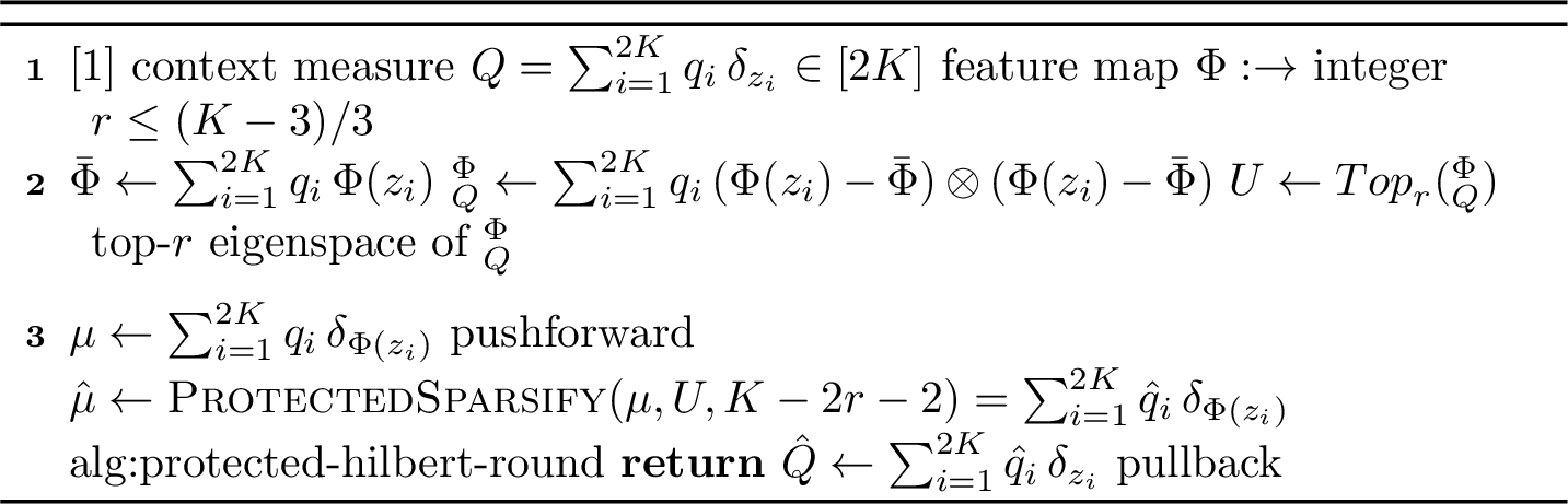

10.2.1 Perfect admissibility via constrained rounding↩︎
6 is a direct implementation of the Hilbert-space sparsification argument in 8. Given a context measure \(Q \in \kvmeasures[2K]\), the reducer preserves the features \(\Phi\) exactly in the leading eigenspace of \(\Sigma_Q^\Phi\), and sparsifies the measure only in the orthogonal complement. Because of that, the reducer is \((\Phi,r,0)\)-admissible.
Theorem 2. Fix \(K\ge 3\) and \(r\le (K-3)/3\). Let \(\mathcal{H}\) be a Hilbert space and \(\Phi: \mathcal{X}\to \mathcal{H}\) bounded. Then, \(\mathrm{\small RoundReduce}(\cdot,\Phi,r)\) is \((\Phi,r,0)\)-admissible.
Proof. Fix \[Q = \sum_{i=1}^{2K} q_i \, \delta_{z_i} \in \kvmeasures[2K],\] set \(m \mathrel{\vcenter{:}}= K-2r-2\), and use the notation of 6. Since \(r\le (K-3)/3\), we have \(m \ge K/3\).
\(\mathrm{\small RoundReduce}(Q,\Phi,r)\) applies \(\mathrm{\small ProtectedSparsify}\) to the pushforward \[\mu = \sum_{i=1}^s q_i\delta_{\Phi(z_i)}\] with protected subspace \[U = \operatorname{Top}_r(\Sigma_Q^\Phi)\] and sparsification budget \(m\).
By [pro:protected-sparsification], \[|\mathop{\mathrm{supp}}(\hat{Q})| \le m+2\dim(U)+2 \le K\] almost surely, and \(\mathop{\mathrm{supp}}(\hat{Q})\subseteq\mathop{\mathrm{supp}}(Q)\). Hence, \[\hat{Q}\in\mathcal{P}_K(\mathop{\mathrm{supp}}(Q)).\] [pro:protected-sparsification] also gives \(\mathop{\mathrm{\mathbb{E}}}[\hat{\mu}]=\mu\) and therefore \(\mathop{\mathrm{\mathbb{E}}}[\hat{Q}]=Q\). That proves unbiasedness.
Let \(\mathcal{G}\) be a Hilbert space and let \(\Psi:\mathcal{X}\to\mathcal{G}\) be bounded. Applying the variance bound in [pro:protected-sparsification] with \(y_i=\Psi(z_i)\) gives \[\mathop{\mathrm{\mathbb{E}}}\Bigl\| \int_{\mathcal{X}}\Psi\,d(\hat{Q}-Q) \Bigr\|_{\mathcal{G}}^2 \le \frac{20}{9m}\mathop{\mathrm{tr}}(\Sigma_Q^\Psi) \le \frac{20}{3K}\mathop{\mathrm{tr}}(\Sigma_Q^\Psi).\]
For the feature map \(\Phi\), let \[\eta_\Phi \mathrel{\vcenter{:}}= \int_{\mathcal{X}}\Phi \mathop{}\!\mathrm{d}(\hat{Q}-Q).\] By the protected covariance bound in [pro:protected-sparsification], \[\mathop{\mathrm{\mathbb{E}}}[\eta_\Phi\otimes\eta_\Phi] \preceq \frac{20}{9m} (I-\Pi_U)\Sigma_Q^\Phi(I-\Pi_U).\] Taking traces and using \(U=\operatorname{Top}_r(\Sigma_Q^\Phi)\), we obtain \[\mathop{\mathrm{\mathbb{E}}}\Bigl\| \int_{\mathcal{X}}\Phi \mathop{}\!\mathrm{d}(\hat{Q}-Q) \Bigr\|_{\mathcal{H}}^2 \le \frac{20}{9m}\mathop{\mathrm{tail}}_r(\Sigma_Q^\Phi) \le \frac{20}{3K}\mathop{\mathrm{tail}}_r(\Sigma_Q^\Phi).\]
Thus, all design criteria hold for every \(Q \in \mathcal{P}_{2K}(X)\), making \(\mathrm{\small RoundReduce}(\cdot,\Phi,r)\) \((\Phi,r,0)\)-admissible. ◻
10.2.2 Practical admissibility via clustering↩︎
7 provides an admissible reducer based on clustering. On a context measure \(Q\), the algorithm protects the principal directions of \(\Sigma_Q^\Phi\) by projecting the features onto the leading eigenspace of \(\Sigma_Q^\Phi\) and clustering them in these protected coordinates.
For the clustering step, any finite-dimensional clustering subroutine \(\mathrm{\small ClusterSlots}\) can be used, provided it produces a balanced latent-slot assignment. Concretely, using the notation of 7, the subroutine receives the weighted protected coordinates \((p_i,u_i)_{i\in L}\), where \(p_i=q_i/\rho\), and returns a matrix \(X \in [0,1]^{m\times |L|}\). Row \(a\) of \(X\) is the sampling distribution used by latent slot \(a\), while the column constraints ensure that each light atom receives the correct expected mass. Formally, \(X\) must satisfy \[\sum_{i\in L}X_{ai}=1 \qquad \text{and} \qquad \sum_{a=1}^m X_{ai}=p_i.\]
For example, one might use weighted k-means to group nearby protected coordinates and then sample representatives from those groups in proportion to their total mass, with \(X\) recording the resulting sampling probabilities.
Naturally, the quality of the compressed summary depends on the quality of the clustering. Using the notation of 7, define the clustering error of the call to ClusterSlots by \[\mathcal{C}(Q) \mathrel{\vcenter{:}}= \frac{1}{K} \sum_{a=1}^m\sum_{i\in L} X_{ai}\|u_i-\bar u_a\|_{\mathcal{H}}^2, \qquad \bar u_a \mathrel{\vcenter{:}}= \sum_{i\in L}X_{ai}u_i.\] If the light mass is zero, we set \(\mathcal{C}_{\mathrm{\small ClusterSlots}}(Q)=0\).
When this clustering error is small, ClusterReduce is admissible, as the following theorem shows.
Theorem 3. Fix \(K \ge 1\) and \(r \ge 0\). Let \(\mathcal{H}\) be a Hilbert space and \(\Phi: \mathcal{X}\to \mathcal{H}\) bounded. Assume that \(\mathrm{\small ClusterSlots}\) satisfies \(\mathcal{C}(Q)\le \tau\) for every input \(Q\in\kvmeasures[2K]\). Then, \(\mathrm{\small ClusterReduce}(\cdot,\Phi,r)\) is \((\Phi,r,\tau)\)-admissible.
Proof. Let \[Q=\sum_{i=1}^{2K}q_i\delta_{z_i}\in\kvmeasures[2K].\]
Use the notation of 7. If the light mass is zero, then \(Q\) must already belong to \(\kvmeasures[K]\). The algorithm then returns \(Q\) exactly, so all claims are immediate.
Assume therefore that \(\beta>0\). Since each \(i\in H\) satisfies \(q_i>1/K\), \[\beta = 1-\sum_{i\in H}q_i < 1-\frac{|H|}{K} = \frac{K-|H|}{K} = \frac{m}{K}.\] Thus, \(\rho=\frac{\beta}{m}\le \frac{1}{K}\)
The output is supported on \(\mathop{\mathrm{supp}}(Q)\) and uses at most \(|H|+m=K\) atoms, so \(\hat{Q}\in\mathcal{P}_K(\mathop{\mathrm{supp}}(Q))\) almost surely. Moreover, the heavy atoms are kept exactly, and for every \(i\in L\), \[\mathop{\mathrm{\mathbb{E}}}[\text{mass assigned to }z_i] = \rho\sum_{a=1}^m X_{ai} = \rho p_i = q_i.\] Hence \(\mathop{\mathrm{\mathbb{E}}}[\hat{Q}]=Q\). That proves unbiasedness.
Let \(\mathcal{G}\) be a Hilbert space and let \(\Psi:\mathcal{X}\to\mathcal{G}\) be bounded. Write \[y_i \mathrel{\vcenter{:}}= \Psi(z_i), \qquad \bar y \mathrel{\vcenter{:}}= \int_{\mathcal{X}}\Psi \mathop{}\!\mathrm{d}Q.\] The heavy atoms contribute no error, while the light slots give \[\int_{\mathcal{X}}\Psi \mathop{}\!\mathrm{d}(\hat{Q}-Q) = \rho\sum_{a=1}^m \left( y_{I_a}-\sum_{i\in L}X_{ai}y_i \right).\] The summands are independent and centered. Therefore \[\begin{align} \mathop{\mathrm{\mathbb{E}}}\left[ \left\| \int_{\mathcal{X}}\Psi \mathop{}\!\mathrm{d}(\hat{Q}-Q) \right\|_{\mathcal{G}}^2 \right] &= \rho^2 \sum_{a=1}^m \mathop{\mathrm{\mathbb{E}}}\left\| y_{I_a}-\sum_{i\in L}X_{ai}y_i \right\|_{\mathcal{G}}^2 \\ &\le \rho^2 \sum_{a=1}^m\sum_{i\in L} X_{ai}\|y_i-\bar y\|_{\mathcal{G}}^2 \\ &= \rho^2 \sum_{i\in L} p_i\|y_i-\bar y\|_{\mathcal{G}}^2 \\ &= \rho \sum_{i\in L} q_i\|y_i-\bar y\|_{\mathcal{G}}^2 \\ &\le \frac{1}{K} \sum_{i=1}^{2K} q_i\|y_i-\bar y\|_{\mathcal{G}}^2 \\ &= \frac{1}{K}\mathop{\mathrm{tr}}(\Sigma_Q^\Psi). \end{align}\] This proves the universal trace criterion.
It remains to prove the distinguished \(\Phi\)-criterion. Let \[x_i \mathrel{\vcenter{:}}= \Phi(z_i), \qquad \bar x \mathrel{\vcenter{:}}= \int_{\mathcal{X}}\Phi \mathop{}\!\mathrm{d}Q, \qquad \xi_i \mathrel{\vcenter{:}}= x_i-\bar x,\] and let \[U \mathrel{\vcenter{:}}= \operatorname{Top}_r(\Sigma_Q^\Phi).\] Then, \(u_i = \Pi_U\xi_i\) for all \(i \in L\). As above, \[\eta_\Phi \mathrel{\vcenter{:}}= \int_{\mathcal{X}}\Phi \mathop{}\!\mathrm{d}(\hat{Q}-Q) = \rho\sum_{a=1}^m \left( \xi_{I_a}-\sum_{i\in L}X_{ai}\xi_i \right).\] Decomposing orthogonally along \(U\oplus U^\perp\), the protected part is \[\mathop{\mathrm{\mathbb{E}}}\|\Pi_U\eta_\Phi\|_{\mathcal{H}}^2 = \rho^2 \sum_{a=1}^m\sum_{i\in L} X_{ai}\|u_i-\bar u_a\|_{\mathcal{H}}^2.\] By the definition of \(\mathcal{C}(Q)\) and \(\rho\le 1/K\), \[\mathop{\mathrm{\mathbb{E}}}\|\Pi_U\eta_\Phi\|_{\mathcal{H}}^2 = \rho^2 K\,\mathcal{C}(Q) \le \frac{\mathcal{C}(Q)}{K} \le \frac{\tau}{K}.\] For the residual part, the same variance estimate used above gives \[\begin{align} \mathop{\mathrm{\mathbb{E}}}\|(I-\Pi_U)\eta_\Phi\|_{\mathcal{H}}^2 &\le \rho \sum_{i\in L} q_i\|(I-\Pi_U)\xi_i\|_{\mathcal{H}}^2 \\&\le \frac{1}{K} \mathop{\mathrm{tr}}\!\left((I-\Pi_U)\Sigma_Q^\Phi\right). \end{align}\] Since \(U=\operatorname{Top}_r(\Sigma_Q^\Phi)\), \[\mathop{\mathrm{tr}}\!\left((I-\Pi_U)\Sigma_Q^\Phi\right) = \mathop{\mathrm{tail}}_r(\Sigma_Q^\Phi).\] Combining the protected and residual parts yields \[\mathop{\mathrm{\mathbb{E}}}\left[ \left\| \int_{\mathcal{X}}\Phi \mathop{}\!\mathrm{d}(\hat{Q}-Q) \right\|_{\mathcal{H}}^2 \right] \le \frac{1}{K} \bigl(\mathop{\mathrm{tail}}_r(\Sigma_Q^\Phi)+\tau\bigr).\]
Thus, all design criteria hold for every \(Q \in \mathcal{P}_{2K}(X)\), making \(\mathrm{\small ClusterReduce}(\cdot,\Phi,r)\) \((\Phi,r,\tau)\)-admissible. ◻
10.3 Global risk guarantees↩︎
This section proves the risk guarantee of [thm:alg-risk] for the chunked prefill and decoding algorithms. Both schedules build summaries in a merge-reduce tree: starting from token chunks of \(K\) tokens, disjoint summaries are merged, their weighted union is compressed back to \(K\) atoms, and the unfinished current chunk is appended exactly. We show that, for admissible local compressors \(\mathop{\mathrm{\mathsf{REDUCE}}}\), the approximation error accumulates linearly with the depth of the merge-reduce tree, which then transfers to the claimed risk guarantees.
10.3.1 Geometry transfer↩︎
\(\mathop{\mathrm{\mathsf{REDUCE}}}\) is designed in the fixed reference geometry induced by \(\Phi: \mathcal{X}\to \mathcal{H}\). In contrast, the desired risk bound is expressed in the geometry induced by \(\Gamma_P: \mathcal{X}\to\mathcal{H}_\nu\), which depends on both the exact context \(P\) and the query distribution \(\nu\). We record here the transfer guarantees from the covariance \(\Sigma^\Phi_P\) in \(\mathcal{H}\) to the covariance \(\Sigma_{P,\nu}\) in \(\mathcal{H}_\nu\). Concretely, 10 shows that, under [asp:common-geometry], the spectral decay of \(\Sigma_P^\Phi\) is controlled by the spectral decay of \(\Sigma_{P,\nu}\) in the reference geometry of \(\Phi\).
Lemma 10. Suppose [asp:common-geometry] holds for \(P,\nu\) and the chosen feature map \(\Phi\). Then, \[\mathop{\mathrm{tail}}_r(\Sigma_P^\Phi) \lesssim \mathop{\mathrm{tail}}_r(\Sigma_{P,\nu})\] for every \(r\ge 0\).
Proof. Let \[\textstyle L_0^2(P) \mathrel{\vcenter{:}}= \left\{f \in L^2(P) \mid \int_\mathcal{X}f \mathop{}\!\mathrm{d}P=0\right\}\] and define \[\textstyle T_\Phi f \mathrel{\vcenter{:}}= \int_\mathcal{X}f(\Phi-\mu_P^\Phi) \mathop{}\!\mathrm{d}P, \qquad T_\Gamma f \mathrel{\vcenter{:}}= \int_\mathcal{X}f\Gamma_P \mathop{}\!\mathrm{d}P .\] Since \(fP\) is a signed, zero-mass measure supported on \(\mathop{\mathrm{supp}}(P)\), [asp:common-geometry] gives \[\|T_\Phi f\|_{\mathcal{H}}^2 \lesssim \|T_\Gamma f\|_{\mathcal{H}_\nu}^2\] for all \(f\in L_0^2(P)\). Equivalently, \[T_\Phi^*T_\Phi \preceq C\,T_\Gamma^*T_\Gamma .\] for a universal constant \(C > 0\). Moreover, \[T_\Phi T_\Phi^*=\Sigma_P^\Phi \qquad \text{and} \qquad T_\Gamma T_\Gamma^*=\Sigma_{P,\nu},\] where the second identity uses \(\int\Gamma_P\,dP=0\). Since \(TT^*\) and \(T^*T\) have the same eigenvalues, \[\mathop{\mathrm{tail}}_r(\Sigma_P^\Phi) = \mathop{\mathrm{tail}}_r(T_\Phi^*T_\Phi) \lesssim \mathop{\mathrm{tail}}_r(T_\Gamma^*T_\Gamma) = \mathop{\mathrm{tail}}_r(\Sigma_{P,\nu}). \tag*{\qedhere}\] ◻
10.3.2 Risk propagation through merge-reduce trees↩︎
We now turn the one-step guarantees of \(\mathop{\mathrm{\mathsf{REDUCE}}}\) into guarantees for full causal prefixes. To that end, we show that the design criteria in [def:admissible-reducer] for \(\mathop{\mathrm{\mathsf{REDUCE}}}\) — unbiasedness of the summary and second-moment control of its feature defect — propagate through the merge-reduce recursion. To express this invariant, we introduce the notion of a valid summary, which is a random context measure of a token block that satisfies the same criteria, with a parameter counting the number of reducer layers on its dependency path. Each node of the merge-reduce tree preserves validity, increasing this parameter by at most one. The global risk bound in [thm:alg-risk] then follows by recognizing the prefill and decoding summaries as outputs of such trees, whose depth is logarithmic in the number of completed chunks.
Definition 6 (Valid summary). Let \(d,r,\tau \ge 0\) and \(A \subseteq \mathbb{N}\). We say that a random context measure \(S_A\) is \((d,r,\tau)\)-valid* for \(A\) if the following hold:*
\(\mathop{\mathrm{\mathbb{E}}}[S_A] = P_A\)
\(\mathop{\mathrm{\mathbb{E}}}\bigl[\|\int_{\mathcal{X}}\Psi \mathop{}\!\mathrm{d}(S_A-P_A)\|_{\mathcal{G}}^2\bigr] \lesssim \frac{d}{K} \mathop{\mathrm{tr}}(\Sigma_{P_A}^\Psi)\) for all Hilbert spaces \(\mathcal{G}\) and bounded \(\Psi: \mathcal{X}\to\mathcal{G}\)
\(\mathop{\mathrm{\mathbb{E}}}\bigl[\|\int_{\mathcal{X}}\Phi \mathop{}\!\mathrm{d}(S_A-P_A)\|_{\mathcal{H}}^2\bigr] \lesssim \frac{d}{K} \bigl(\mathop{\mathrm{tail}}_r(\Sigma_{P_A}^\Phi) + \tau \bigr)\)
Note that this resembles directly the design criteria of a \((\Phi,r,\tau)\)-admissible reducer, as defined in [def:admissible-reducer]. In particular, if \(\mathop{\mathrm{\mathsf{REDUCE}}}\) is \((\Phi,r,\tau)\)-admissible and \(P_A \in \kvmeasures[2K]\) is the context measure of the tokens in \(A \subseteq \mathbb{N}\), then \(\mathop{\mathrm{\mathsf{REDUCE}}}(P_A)\) is \((1,r,\tau)\)-valid for \(A\).
We briefly record the following fact that we use repeatedly later on.
Lemma 11. Let \(P \in \kvmeasures\) and let \(Q\) be a random variable taking values in \(\kvmeasures\). If \(\mathop{\mathrm{\mathbb{E}}}[Q] = P\), then \(\mathop{\mathrm{\mathbb{E}}}[\Sigma^\Psi_Q] \preceq \Sigma^\Psi_P\) for any Hilbert space \(\mathcal{G}\) and bounded \(\Psi: \mathcal{X}\to \mathcal{G}\).
Proof. Let \(\mathcal{G}\) be a Hilbert space and \(\Psi: \mathcal{X}\to \mathcal{G}\) be bounded. Then, \[\begin{align} \mathop{\mathrm{\mathbb{E}}}\!\left[\Sigma_{Q}^\Psi\right] &= \mathop{\mathrm{\mathbb{E}}}\!\left[ \int_\mathcal{X}\Psi \otimes \Psi \mathop{}\!\mathrm{d}Q \right] - \mathop{\mathrm{\mathbb{E}}}\!\left[ \mu_Q^\Psi \otimes \mu_Q^\Psi \right] \\&= \int_\mathcal{X}\Psi \otimes \Psi \mathop{}\!\mathrm{d}P - \mathop{\mathrm{\mathbb{E}}}\!\left[ \mu_Q^\Psi \otimes \mu_Q^\Psi \right] \\&= \int_\mathcal{X}\Psi \otimes \Psi \mathop{}\!\mathrm{d}P - \mathop{\mathrm{\mathbb{E}}}\!\left[ \left(\mu_Q^\Psi - \mathop{\mathrm{\mathbb{E}}}\!\left[\mu_Q^\Psi\right]\right) \otimes \left(\mu_Q^\Psi - \mathop{\mathrm{\mathbb{E}}}\!\left[\mu_Q^\Psi\right]\right) \right] - \mathop{\mathrm{\mathbb{E}}}\!\left[\mu_Q^\Psi\right] \otimes \mathop{\mathrm{\mathbb{E}}}\!\left[\mu_Q^\Psi\right] \\&= \int_\mathcal{X}\Psi \otimes \Psi \mathop{}\!\mathrm{d}P - \mathop{\mathrm{\mathbb{E}}}\!\left[ \left(\mu_Q^\Psi - \mu_P^\Psi\right) \otimes \left(\mu_Q^\Psi - \mu_P^\Psi\right) \right] - \mu_P^\Psi \otimes \mu_P^\Psi \\&= \Sigma_P^\Psi - \mathop{\mathrm{\mathbb{E}}}\!\left[ \left(\mu_Q^\Psi - \mu_P^\Psi\right) \otimes \left(\mu_Q^\Psi - \mu_P^\Psi\right) \right] \\&\preceq \Sigma_P^\Psi. \tag*{\qedhere} \end{align}\] ◻
We now consider the operation at a single node in the merge-reduce tree. Given two summaries of two disjoint blocks of tokens, we form a compressed summary of their union by compressing their weighted combination using \(\mathop{\mathrm{\mathsf{REDUCE}}}\). When the two input summaries are \((d,r,\tau)\)-valid, the resulting summary is \((d+1,r,\tau)\)-valid, thereby propagating the guarantees up the merge-reduce tree.
Lemma 12. Let \(A,B \subseteq \mathbb{N}\) be finite, nonempty, and disjoint. Let \(S_A\) be \((d_A,r,\tau)\)-valid for \(A\), and let \(S_B\) be \((d_B,r,\tau)\)-valid for \(B\). Assume that \(\mathop{\mathrm{\mathsf{REDUCE}}}\) is \((\Phi,r,\tau)\)-admissible and that \(S_A\) and \(S_B\) are independent. Define \[Q \mathrel{\vcenter{:}}= \frac{w(A)}{w(A)+w(B)} S_A + \frac{w(B)}{w(A)+w(B)} S_B.\] If \(Q\in\kvmeasures[2K]\), then \(\mathop{\mathrm{\mathsf{REDUCE}}}(Q)\) is \((1+\max\{d_A,d_B\},r,\tau)\)-valid for \(A\cup B\).
Proof. Let \(S_{A \cup B} \mathrel{\vcenter{:}}= \mathop{\mathrm{\mathsf{REDUCE}}}(Q)\), and write \[P\mathrel{\vcenter{:}}= P_{A\cup B} = \alpha P_A+\beta P_B\] for \(\alpha \mathrel{\vcenter{:}}= w(A) / (w(A) + w(B))\) and \(\beta \mathrel{\vcenter{:}}= w(B) / (w(A) + w(B))\). Additionally, introduce the defects \[\sigma_A \mathrel{\vcenter{:}}= S_A - P_A ,\qquad \sigma_B \mathrel{\vcenter{:}}= S_B - P_B ,\qquad \sigma_{A \cup B} \mathrel{\vcenter{:}}= S_{A \cup B} - P_{A \cup B},\] and \[\eta \mathrel{\vcenter{:}}= S_{A \cup B} - Q\] which are all zero-mass, signed measures on \(\mathcal{X}\).
For a Hilbert space \(\mathcal{G}\) and bounded \(\Psi: \mathcal{X}\to \mathcal{G}\), introduce the notation \[\Psi[\sigma] \mathrel{\vcenter{:}}= \int_\mathcal{X}\Psi \mathop{}\!\mathrm{d}\sigma\] for zero-mass, signed measures \(\sigma\) on \(\mathcal{X}\).
We next prove orthogonality of the defects after taking expectation. Condition on the already constructed summaries \(S_A,S_B\). Then \(Q\), \(\sigma_A\), and \(\sigma_B\) are fixed, and the only remaining randomness is the fresh call to \(\mathop{\mathrm{\mathsf{REDUCE}}}\). Admissibility of \(\mathop{\mathrm{\mathsf{REDUCE}}}\) gives \(\mathop{\mathrm{\mathbb{E}}}[\eta\mid S_A,S_B]=0\). Hence, \[\mathop{\mathrm{\mathbb{E}}}\bigl[\langle \Psi[\eta], \Psi[\sigma_A] \rangle_\mathcal{G}\bigr] = \mathop{\mathrm{\mathbb{E}}}\bigl[\langle \mathop{\mathrm{\mathbb{E}}}[\Psi[\eta] \mid S_A, S_B], \Psi[\sigma_A] \rangle_\mathcal{G}\bigr] = 0,\] and similarly for \(\mathop{\mathrm{\mathbb{E}}}[\langle \Psi[\eta], \Psi[\sigma_B] \rangle_\mathcal{G}]\). Moreover, \(S_A\) and \(S_B\) are independent and validity of \(S_A\) and \(S_B\) imply \[\mathop{\mathrm{\mathbb{E}}}[\Psi[\sigma_A]] = \mathop{\mathrm{\mathbb{E}}}[\Psi[\sigma_B]] = 0.\] Therefore, \[\mathop{\mathrm{\mathbb{E}}}\bigl[\langle \Psi[\sigma_A], \Psi[\sigma_B] \rangle_\mathcal{G}\bigr] = \bigl\langle \mathop{\mathrm{\mathbb{E}}}\bigl[\Psi[\sigma_A]\bigr], \mathop{\mathrm{\mathbb{E}}}\bigl[\Psi[\sigma_B]\bigr] \bigr\rangle_\mathcal{G} = 0\] and thus expanding the square norm gives \[\label{eq:one-merge-validity:pythagoras} \mathop{\mathrm{\mathbb{E}}}\bigl\|\Psi[\sigma_{A \cup B}]\bigr\|_\mathcal{G}^2 = \mathop{\mathrm{\mathbb{E}}}\bigl\|\Psi[\eta]\bigr\|_\mathcal{G}^2 + \alpha^2 \, \mathop{\mathrm{\mathbb{E}}}\bigl\|\Psi[\sigma_A]\bigr\|_\mathcal{G}^2 + \beta^2 \, \mathop{\mathrm{\mathbb{E}}}\bigl\|\Psi[\sigma_B]\bigr\|_\mathcal{G}^2.\tag{9}\]
We now prove the three validity conditions for \(S_{A \cup B}\).
For unbiasedness, \[\mathop{\mathrm{\mathbb{E}}}[S_{A\cup B}] = \mathop{\mathrm{\mathbb{E}}}[\mathop{\mathrm{\mathbb{E}}}[\mathop{\mathrm{\mathsf{REDUCE}}}(Q)\mid S_A,S_B]] = \mathop{\mathrm{\mathbb{E}}}[Q] = \alpha P_A+\beta P_B = P,\] which follows immediately from unbiasedness of \(S_A\) and \(S_B\).
For trace control, we bound the three terms in 9 . Fix a Hilbert space \(\mathcal{G}\) and a bounded map \(\Psi: \mathcal{X}\to \mathcal{G}\). Since \(\mathop{\mathrm{\mathbb{E}}}[Q]=P\), 11 gives \(\mathop{\mathrm{\mathbb{E}}}[\Sigma^\Psi_Q]\preceq \Sigma^\Psi_P\). Conditioning on \(S_A,S_B\), the input \(Q\) is fixed and the remaining randomness is the fresh reducer randomness. Thus, admissibility of \(\mathop{\mathrm{\mathsf{REDUCE}}}\) gives \[\mathop{\mathrm{\mathbb{E}}}\bigl[\bigl\| \Psi[\eta] \bigr\|_\mathcal{G}^2 \bigm| S_A,S_B \bigr] \lesssim \frac{1}{K}\mathop{\mathrm{tr}}\bigl(\Sigma_Q^\Psi\bigr).\] Taking expectations, \[\mathop{\mathrm{\mathbb{E}}}\bigl\| \Psi[\eta] \bigr\|_\mathcal{G}^2 \lesssim \frac{1}{K}\mathop{\mathrm{\mathbb{E}}}\mathop{\mathrm{tr}}\bigl(\Sigma_Q^\Psi\bigr) \le \frac{1}{K}\mathop{\mathrm{tr}}\bigl(\Sigma_P^\Psi\bigr).\]
By validity of \(S_A\) and \(S_B\), \[\begin{align} \alpha^2\mathop{\mathrm{\mathbb{E}}}\bigl\|\Psi[\sigma_A]\bigr\|_{\mathcal{G}}^2 + \beta^2\mathop{\mathrm{\mathbb{E}}}\bigl\|\Psi[\sigma_B]\bigr\|_{\mathcal{G}}^2 &\lesssim \frac{\max\{d_A,d_B\}}{K} \Bigl[ \alpha^2\mathop{\mathrm{tr}}(\Sigma^\Psi_{P_A}) + \beta^2\mathop{\mathrm{tr}}(\Sigma^\Psi_{P_B}) \Bigr] \\&\le \frac{\max\{d_A,d_B\}}{K} \Bigl[\mathop{\mathrm{tr}}\bigl(\alpha \Sigma^\Psi_{P_A} + \beta \Sigma^\Psi_{P_B}\bigr)\Bigr] \\&\le \frac{\max\{d_A,d_B\}}{K} \Bigl[\mathop{\mathrm{tr}}\bigl(\Sigma^\Psi_P\bigr)\Bigr], \end{align}\] where we additionally use \(\alpha^2\le\alpha\), \(\beta^2\le\beta\), and \(\alpha \Sigma^\Psi_{P_A}+\beta \Sigma^\Psi_{P_B}\preceq \Sigma^\Psi_P\) by 11. Combining this with 9 and admissibility of \(\mathop{\mathrm{\mathsf{REDUCE}}}\) proves \[\mathop{\mathrm{\mathbb{E}}}\bigl\| \Psi[\sigma_{A \cup B}] \bigr\|_\mathcal{G}^2 \lesssim \left(\frac{1+\max\{d_A,d_B\}}{K}\right) \mathop{\mathrm{tr}}\bigl(\Sigma^\Psi_P\bigr).\] Since \(\Psi\) and \(\mathcal{G}\) were arbitrary, that proves the trace condition.
For tail control, condition on \(S_A,S_B\). Then, \(Q\) is fixed and the remaining randomness is the fresh reducer randomness. Admissibility applied to this realized input \(Q\) gives \[\mathop{\mathrm{\mathbb{E}}}\!\left[\|\Phi[\eta]\|_{\mathcal{H}}^2 \bigm| S_A,S_B\right] \lesssim \frac{1}{K} \left(\mathop{\mathrm{tail}}_r(\Sigma^\Phi_Q)+\tau\right).\] Taking expectations gives \[\mathop{\mathrm{\mathbb{E}}}\|\Phi[\eta]\|_{\mathcal{H}}^2 \lesssim \frac{1}{K} \left(\mathop{\mathrm{\mathbb{E}}}[\mathop{\mathrm{tail}}_r(\Sigma^\Phi_Q)]+\tau\right).\] Since \(\mathop{\mathrm{\mathbb{E}}}[Q]=P\), 11 gives \(\mathop{\mathrm{\mathbb{E}}}[\Sigma^\Phi_Q]\preceq \Sigma^\Phi_P\). By concavity and monotonicity of \(\mathop{\mathrm{tail}}_r\), \[\mathop{\mathrm{\mathbb{E}}}[\mathop{\mathrm{tail}}_r(\Sigma^\Phi_Q)] \le \mathop{\mathrm{tail}}_r(\mathop{\mathrm{\mathbb{E}}}[\Sigma^\Phi_Q]) \le \mathop{\mathrm{tail}}_r(\Sigma^\Phi_P).\] Hence \[\mathop{\mathrm{\mathbb{E}}}\|\Phi[\eta]\|_{\mathcal{H}}^2 \lesssim \frac{1}{K} \bigl(\mathop{\mathrm{tail}}_r(\Sigma^\Phi_P)+\tau\bigr).\] By validity of \(S_A\) and \(S_B\), \[\begin{align} \alpha^2\mathop{\mathrm{\mathbb{E}}}\bigl\|\Phi[\sigma_A]\bigr\|_{\mathcal{H}}^2 + \beta^2\mathop{\mathrm{\mathbb{E}}}\bigl\|\Phi[\sigma_B]\bigr\|_{\mathcal{H}}^2 &\lesssim \frac{\max\{d_A,d_B\}}{K} \Bigl[ \alpha^2(\mathop{\mathrm{tail}}_r(\Sigma^\Phi_{P_A})+\tau) + \beta^2(\mathop{\mathrm{tail}}_r(\Sigma^\Phi_{P_B})+\tau) \Bigr] \\&\le \frac{\max\{d_A,d_B\}}{K} \Bigl[ \alpha \, \mathop{\mathrm{tail}}_r(\Sigma^\Phi_{P_A}) + \beta \, \mathop{\mathrm{tail}}_r(\Sigma^\Phi_{P_B}) + \tau \Bigr] \\&\le \frac{\max\{d_A,d_B\}}{K} \Bigl[\mathop{\mathrm{tail}}_r\bigl(\Sigma^\Phi_P\bigr) + \tau\Bigr], \end{align}\] where we additionally use \(\alpha^2\le\alpha\), \(\beta^2\le\beta\), \(\alpha \Sigma^\Phi_{P_A}+\beta \Sigma^\Phi_{P_B}\preceq \Sigma^\Phi_P\) by 11, and concavity of \(\mathop{\mathrm{tail}}_r\). Plugging into 9 , we get \[\mathop{\mathrm{\mathbb{E}}}\bigl\|\Phi[\sigma_{A \cup B}]\bigr\|_{\mathcal{H}}^2 \lesssim \frac{1+\max\{d_A,d_B\}}{K} \bigl(\mathop{\mathrm{tail}}_r(\Sigma^\Phi_P)+\tau\bigr).\] That proves the tail condition. Hence, \(S_{A\cup B}\) is \((1+\max\{d_A,d_B\},r,\tau)\)-valid for \(A\cup B\). ◻
Validity of a summary gives us the desired risk control, but only in terms of the fixed geometry of \(\mathcal{H}\). [pro:algorithm-risk] transfers this control to the attention error, which is measured in the geometry of \(\mathcal{H}_\nu\).
Fix \(\nu\in\mathcal{P}(\mathcal{Q})\), and let \(\hat{P}_t\) be a random context measure. If \(\hat{P}_t\) is \((d_t,r,\tau)\)-valid for \(\{1,\ldots,t\}\), then \[\mathop{\mathrm{\mathbb{E}}}\bigl[\err*{P_t}{\nu}{\hat{P}_t}\bigr] \lesssim \frac{d_t}{K}\mathop{\mathrm{tr}}(\Sigma_{P_t,\nu}).\] If additionally \((P_t,\nu)\) satisfies [asp:common-geometry], then \[\mathop{\mathrm{\mathbb{E}}}\bigl[\err*{P_t}{\nu}{\hat{P}_t}\bigr] \lesssim \frac{d_t}{K} \left(\mathop{\mathrm{tail}}_r(\Sigma_{P_t,\nu}) + \tau\right).\]
Proof. First, note that \[\label{eq:algorithm-risk:transfer} \err*{P_t}{\nu}{\hat{P}_t} \overset{(1)}{\lesssim} \left\| \int_{\mathcal{X}}\Gamma_{P_t} \mathop{}\!\mathrm{d}\hat{P}_t \right\|_{\mathcal{H}_\nu}^2 \overset{(2)}{=} \left\| \int_{\mathcal{X}}\Gamma_{P_t} \mathop{}\!\mathrm{d}(\hat{P}_t - P_t) \right\|_{\mathcal{H}_\nu}^2\tag{10}\] where \((1)\) uses 2, and \((2)\) uses \(\int_\mathcal{X}\Gamma_{P_t} \mathop{}\!\mathrm{d}P_t = 0\).
Using validity of \(\hat{P}_t\) applied to \(\Gamma_{P_t}\), it follows that \[\mathop{\mathrm{\mathbb{E}}}\err*{P_t}{\nu}{\hat{P}_t} \lesssim \frac{d_t}{K} \mathop{\mathrm{tr}}(\Sigma_{P_t}^{\Gamma_{P_t}}) = \frac{d_t}{K} \mathop{\mathrm{tr}}(\Sigma_{P_t,\nu}).\] That proves the first claim.
Suppose now that [asp:common-geometry] holds. Then, using validity of \(\hat{P}_t\) and 10, \[\mathop{\mathrm{\mathbb{E}}}\err*{P_t}{\nu}{\hat{P}_t} \overset{\eqref{eq:algorithm-risk:transfer}}{\lesssim} \mathop{\mathrm{\mathbb{E}}}\left\| \int_{\mathcal{X}}\Gamma_{P_t} \mathop{}\!\mathrm{d}(\hat{P}_t - P_t) \right\|_{\mathcal{H}_\nu}^2 \lesssim \frac{d_t}{K} \bigl( \mathop{\mathrm{tail}}_r\bigl(\Sigma_{P_t}^\Phi\bigr) + \tau \bigr) \lesssim \frac{d_t}{K} \bigl( \mathop{\mathrm{tail}}_r(\Sigma_{P_t,\nu}) + \tau \bigr),\] which proves the second claim. ◻
The final summary \(\hat{P}_t\) used as the compressed context for the token at position \(t\) is a combination of a compressed summary produced by the merge-reduce tree and an exact context measure of the tokens inside the same chunk as token \(t\). The next lemma shows that this is harmless for the validity of the resulting summary.
Lemma 13. Let \(A,R \subseteq \mathbb{N}\) be finite and disjoint and \(A \neq \emptyset\). If \(S_A\) is \((d,r,\tau)\)-valid for \(A\), then \[S_{A\cup R} \mathrel{\vcenter{:}}= \frac{w(A)}{w(A)+w(R)}S_A + \frac{w(R)}{w(A)+w(R)}P_R\] is \((d,r,\tau)\)-valid for \(A\cup R\).
Proof. Unbiasedness of \(S_{A \cup R}\) is immediate from unbiasedness of \(S_A\) and \(P_R\). Set \(\alpha \mathrel{\vcenter{:}}= w(A)/(w(A)+w(R))\).
Let \(\mathcal{G}\) be a Hilbert space and \(\Psi: \mathcal{X}\to \mathcal{G}\) bounded. Then, the defect of \(S_{A\cup R}\) is \[\int_\mathcal{X}\Psi \mathop{}\!\mathrm{d}(S_{A \cup R} - P_{A \cup R}) = \alpha \left( \int_\mathcal{X}\Psi \mathop{}\!\mathrm{d}(S_A - P_A) \right)\] Since \(\alpha \Sigma^\Psi_{P_A}\preceq \Sigma^\Psi_{P_{A\cup R}}\), the validity estimates for \(S_A\) imply the validity estimates for \(S_{A\cup R}\). ◻
It remains only to count the validity depth of the summaries produced by [alg:prefill-compression,alg:decoding-compression]. The prefill scan and the decoding buckets both construct summaries by repeated binary merges of disjoint completed chunks. Along any dependency path there are only logarithmically many reducer calls, and the unfinished current chunk is appended exactly. Thus, if \(\mathop{\mathrm{\mathsf{REDUCE}}}\) is \((\Phi,r,\tau)\)-admissible, each resulting prefix summary \(\hat{P}_t\) is \((d,r,\tau)\)-valid, with \(d\) proportional to the depth of the tree, which is logarithmic in the number of tokens. The claimed risk guarantees then follow immediately from [pro:algorithm-risk].
Proof. We first show that \(\hat{P}_t\) as produced by [alg:prefill-compression,alg:decoding-compression] is \(\mathop{\mathrm{\mathcal{O}}}(\log(2+t/K),r,\tau)\)-valid for \(\{1,\ldots,t\}\). The risk bounds then follow immediately from [pro:algorithm-risk].
Let \(I_1,I_2,\ldots\) denote the consecutive chunks of size \(K\), and let \(c(t)\) be the chunk containing \(t\). Write \[A_t \mathrel{\vcenter{:}}= I_1\cup\cdots\cup I_{c(t)-1}, \qquad R_t \mathrel{\vcenter{:}}= I_{c(t)}\cap\{1,\ldots,t\}.\] Thus, \(P_t\) is the normalized mixture of \(P_{A_t}\) and the exact current-chunk suffix \(P_{R_t}\), with the obvious convention when \(A_t=\emptyset\).
We claim that every summary stored by the merge-reduce computation for a union of \(m\) completed chunks is \((O(\log(2+m)),r,\tau)\)-valid for its underlying index set, and that summaries stored on disjoint index sets are independent. This follows by induction on the binary merge tree. A single chunk is represented exactly, hence is deterministic and \((0,r,\tau)\)-valid. Whenever two disjoint summaries with validity \(d_1\) and \(d_2\) are merged, the induction hypothesis gives their independence; the reducer call uses fresh randomness independent of both summaries. Thus, 12 shows that the resulting summary is \(((1+\max\{d_1,d_2\}),r,\tau)\)-valid. The resulting summary depends only on its two children and on the fresh randomness used in this reducer call, so it remains independent of all stored summaries supported on disjoint index sets. Along any path in the merge tree for \(m\) chunks there are at most \(\mathop{\mathrm{\mathcal{O}}}(\log(2+m))\) merges. Hence the summary of any completed-chunk prefix produced by the prefill scan, and the completed-prefix summary maintained by the decoding buckets, is \((\mathop{\mathrm{\mathcal{O}}}(\log(2+m)),r,\tau)\)-valid.
Apply this to the completed chunks preceding \(t\). If \(A_t\neq\emptyset\), the algorithm has an \((\mathop{\mathrm{\mathcal{O}}}(\log(2+|A_t|/K)),r,\tau)\)-valid summary \(S_{A_t}\) for \(A_t\). Since \(R_t\) is kept exact, \[\hat{P}_t = \frac{w(A_t)}{w(A_t)+w(R_t)}S_{A_t} + \frac{w(R_t)}{w(A_t)+w(R_t)}P_{R_t}.\] By 13, and using \(|A_t| \le t\), \(\hat{P}_t\) is \((\mathop{\mathrm{\mathcal{O}}}(\log(2+t/K)), r, \tau)\)-valid for \(\{1,\ldots,t\}\).
The claim then follows immediately from [pro:algorithm-risk]. ◻
The global guarantee therefore reduces entirely to the design of \(\mathop{\mathrm{\mathsf{REDUCE}}}\). Any concrete reducer satisfying the one-step trace and tail conditions of [def:admissible-reducer] inherits the same causal prefill and decoding guarantees through the merge-reduce schedules of [alg:prefill-compression,alg:decoding-compression], with only the logarithmic depth loss.
10.4 Computational cost of the global merge-reduce scheme↩︎
We prove [pro:runtime] from the main text.
Proof. Let \(M=n/K\) and \(L=\log_2 M\). We count calls to \(\mathrm{\small Reduce}\) and atom storage, treating each \(K\)-atomic summary as an object of size \(K\).
First, consider Algorithm 2. In the upsweep stage, level \(\ell\) contains \(M/2^\ell\) independent merge-reduce operations. Hence, the number of calls to \(\mathrm{\small Reduce}\) in the upsweep is \[\sum_{\ell=1}^{L} \frac{M}{2^\ell} = M-1 .\] The downsweep has the same count. The total number of calls is thus \(2M-2=\mathop{\mathrm{\mathcal{O}}}(n/K)\).
The parallel depth is also immediate from the tree structure. All calls at a fixed level are independent, so each level contributes one parallel round of \(\mathrm{\small Reduce}\). There are \(L\) upsweep levels and \(L\) downsweep levels, giving depth \(\mathop{\mathrm{\mathcal{O}}}(L)=\mathop{\mathrm{\mathcal{O}}}(\log(n/K))\).
For memory, the algorithm stores \(\mathop{\mathrm{\mathcal{O}}}(M)\) summaries across all levels of the scan tree, and each summary is \(K\)-atomic. Thus the total number of stored atoms is \(\mathop{\mathrm{\mathcal{O}}}(MK)=\mathop{\mathrm{\mathcal{O}}}(n)\).
Now consider Algorithm 3. After \(s\) completed chunks have been incorporated, including the prompt summary, the nonempty buckets satisfy the standard binary-counter invariant: bucket \(B_\ell\), when nonempty, stores a \(K\)-atomic summary of a block of \(2^\ell\) chunks, and there is at most one nonempty bucket at each level. Therefore, the number of nonempty buckets is at most \(1+\lfloor \log_2 s \rfloor\). For a prefix of length \(t=sK\), the number of stored atoms is consequently \[\mathop{\mathrm{\mathcal{O}}}(K\log s)=\mathop{\mathrm{\mathcal{O}}}(K\log(t/K)).\]
It remains to count calls to \(\mathrm{\small Reduce}\). Each new chunk first creates a level-zero bucket. The while loop then performs the carry operations of a binary counter. Whenever a bucket is already occupied, the two \(K\)-atomic summaries are merged and reduced to form one summary at the next level. Over \(s\) chunk insertions, level \(\ell\) participates in at most \(O(s/2^{\ell+1})\) such carries. Summing over \(\ell\) gives \(\mathop{\mathrm{\mathcal{O}}}(s)\) carry calls in total, hence \(\mathop{\mathrm{\mathcal{O}}}(1)\) amortized carry calls per chunk.
After the carry step, the algorithm forms the current history summary by merging the nonempty buckets in decreasing order. Since there are \(\mathop{\mathrm{\mathcal{O}}}(\log s)\) nonempty buckets, this uses \(\mathop{\mathrm{\mathcal{O}}}(\log s)\) calls to \(\mathrm{\small Reduce}\) per completed chunk. Combining this with the \(\mathop{\mathrm{\mathcal{O}}}(1)\) amortized carry cost gives \(\mathop{\mathrm{\mathcal{O}}}(\log s)\) calls per chunk. Since each chunk contains \(K\) tokens, the amortized number of calls per token is \[\mathop{\mathrm{\mathcal{O}}}(\log s/K)=O(\log(t/K)/K).\] That proves the claim. ◻
11 Experimental details↩︎
This appendix describes the implementation of our experiments in 6. Detailed instructions for reproducing our experiments are provided with the code in the supplementary material.
11.0.0.1 Dataset and model.
We evaluate on the “long” subset of LongBench-v2 [24]. The dataset is available at https://longbench2.github.io/. We use the official LongBench-v2 evaluation protocol. We run all experiments on Qwen3-32B [25], using
int4 quantization. We extend the context window to \(131\mathrm{k}\) tokens using YaRN RoPE scaling [27]. The model is available at https://huggingface.co/Qwen/Qwen3-32B. We disable chain-of-thought generation and use greedy decoding throughout. LongBench-v2
and Qwen3-32B are released under the Apache-2.0 license.
11.0.0.2 Computational resources.
All experiments were conducted on a single NVIDIA H100 GPU with \(95{,}830\) MiB VRAM. The full set of runs took approximately 100 GPU hours, including failed runs.
11.0.0.3 Implementation details.
For the full-attention baseline, we use the standard implementation of the Qwen3-32B model. For the compressed methods, we use the algorithms described in 5, with two additions. First, each token may attend to the first \(8\) tokens, following the attention-sink heuristic of [8]. Second, each token may attend to the \(K\) tokens immediately preceding its chunk boundary. Thus, each token attends to at most \(3K+8\) tokens. This is compatible with our theory and enjoys the same guarantees. We use \(K=2048\), corresponding to a compression rate of approximately \(95\%\) relative to the \(131\mathrm{k}\)-token context available to the full-attention baseline.
Many LongBench-v2 contexts exceed even the extended context window of Qwen3-32B. For such examples, we follow the official truncation protocol of [24] by removing the middle section of the prompt.
11.0.0.4 Local reducer instantiations.
We report results for two instantiations of \(\mathop{\mathrm{\mathsf{REDUCE}}}\): random sampling and protected clustering. All randomized methods are evaluated with a single run using a fixed random seed.
For random sampling, we sample i.i.d.from the context measure, i.e., proportionally to \[\label{eq:experiments:weights} \textstyle \exp\!\left(\|k\|_2^2/(2\sqrt{d_k})\right),\tag{11}\] as described in 3.
Protected clustering corresponds to 7, using the static feature map described in 10.1 with the value norm bound fixed to \(V^2=50\). We evaluate protected ranks \(r=64\) and \(r=128\). To compute the leading eigenspace, we use a randomized Nyström approximation with four-fold oversampling.
For ClusterSlots in 7, we use a sliced equal-mass clustering rule. After the heavy atoms have been retained exactly as in 7, the light atoms \(i\in L\) have normalized masses \(p_i=q_i/\rho\) satisfying \(\sum_{i\in L}p_i=m\). For each direction in a fixed bank of random directions in the protected coordinate space, we sort the light atoms by their one-dimensional projection and place intervals of length \(p_i\) consecutively on \([0,m]\). The \(m\) latent slots are the unit intervals of this line, and the assignment matrix \(X\) is given by the overlap of each atom interval with each unit slot. This construction satisfies the row and column constraints required in 7. We choose the direction with the smallest within-slot squared error in the protected coordinates and sample one representative from each slot by inverse-transform sampling.
For this method, we treat the initial context measure as uniform over the tokens rather than proportional to 11 , as this significantly improved numerical stability in the computation of the leading eigenspace.
11.0.0.5 Literature baselines.
We compare performance against ScissorHands [6], SnapKV [9], and StreamingLLM [8]. All three methods use a sliding window of the most recent \(4096\) tokens. The allocation of the remaining \(2056\) token budget is dictated by the respective method. StreamingLLM retains the initial \(8\) sink tokens and uses the rest of this budget to extend the recent-token window. SnapKV retains the top-ranked non-recent prompt tokens by attention score from the final prompt window, using average pooling with kernel size 5, as in the original paper [9]. ScissorHands retains the top-ranked non-recent tokens by cumulative pivotal-token counts.