Asymmetric Trading Prophets
July 01, 2026
Abstract
The “Trading Prophet” problem challenges an online trader to maximize its profit by buying and selling assets under stochastic prices and capacity constraints, competing against an offline prophet with full foresight. In previous work, each arriving asset was assumed to have a single price \(p_t\), and the trader was allowed to either buy a copy at this price (subject to having available capacity), or sell a copy (if it already held at least one copy in hand). However, this abstraction can fail to capture the structural asymmetry of decentralized dealer-based markets, where buying and selling opportunities could be distinct, and driven by individual preferences. To address this, we introduce the Asymmetric Trading Prophets problem, where at each timestep the trader observes a price tuple \((b_t, s_t)\)—representing the cost to buy, and the revenue from selling at this timestep. Importantly, the \((b_t,s_t)\) tuple could be potentially arbitrarily correlated.
We provide the first competitive analysis for this asymmetric trading prophets problem, characterizing the achievable profit based on the trader’s capacity \(B\) and initial inventory \(B_0\). For the unit-capacity case of \(B=1\), we design online algorithms that achieve constant competitive ratios for both i.i.d.and non-i.i.d.distributions on the price tuples, when the trader has one initial copy (\(B_0=1\)). For the general capacity case where \(B\) can be large, we give algorithms for i.i.d. distributions that achieve a competitive ratio of \(1 - \Theta(\log B_0/\sqrt{B_0})\). Finally, for the symmetric case (where the price tuple satisfies \(b_t=s_t\)), we improve this to get a competitive ratio of \(1 - O(\log B/\sqrt{B})\), demonstrating that the performance approaches optimality as the capacity increases. We show that both ratios are tight up to a logarithmic factor.
1 Introduction↩︎
The maxim “buy low, sell high” captures the fundamental goal of any trader, yet executing this strategy in an online setting involves significant uncertainty. This challenge is formally captured by the Trading Prophets problem, introduced by [1]. In this setting, a trader observes a sequence of stochastic prices for the same asset; they must decide, irrevocably and in real-time, whether to buy a copy of the asset (if they have available capacity) or to sell a copy (if they have at least one copy they can sell), to maximize profit within storage constraints. The objective is to design online algorithms that compete against the “prophet”—an offline benchmark with full foresight of future price realizations. This framework bridges the classic theory of prophet inequalities and optimal stopping with the dynamics of inventory management.
The work by [1] and [2] has established strong theoretical foundations for this problem. These works model the market as an exogenous ticker tape: at any time step \(t\), there is a single “market price” drawn from a known distribution. The trader chooses to transact (either buy or sell) at this price. This abstraction effectively models centralized exchanges, such as the stock market, where a unified price dictates terms for all participants and the cost to buy is tightly coupled to the revenue from selling.
However, this “single price” abstraction fails to capture the structural asymmetry inherent in other decentralized or dealer-based markets. In these settings, a trader acts as a market-maker, facing a stream of distinct agents, each with their own private valuations. For instance, in the market for used vehicles, the price at which a dealer can acquire inventory from a desperate seller can be often entirely distinct from the price a collector is willing to pay for that same item, even if they arrive at the same time. Here, the “price” is not a single scalar, but rather a set of distinct buying and selling opportunities driven by individual preferences rather than a unified market signal.
To address this gap, we introduce the Asymmetric Trading Prophet (ATP) problem. In our model, at each time step \(t\), the trader observes a price tuple \((b_t, s_t)\) drawn from a known distribution, where \(b_t\) represents the cost to purchase an item and \(s_t\) represents the revenue from selling one. Crucially, we allow \(b_t\) and \(s_t\) to be arbitrarily correlated. The trader must now perform exactly one of the following actions: buy, sell, or skip. This framework strictly generalizes the “symmetric” stock market model (by setting \(b_t = s_t\)) while capturing scenarios inaccessible to prior works, such as disjoint buy-only or sell-only opportunities (e.g., via \(s_t = 0\) or \(b_t = \infty\)), and general asymmetric price structures. Having formulated this model, we ask:
Question 1: Can we design online algorithms that achieve (expected) profit comparable to the offline optimal prophet in hindsight in the Asymmetric Trading Prophet problem?
The original Trading Prophet model proposed by [1] and [2] assumes that the trader has unit-capacity, and can hold at most one item.5 While this unit-capacity assumption is sufficient for stock markets where inventory can be liquidated instantly, it is restrictive for markets like used vehicles. In such dealer-based settings, buyers and sellers are individuals who arrive sequentially, meaning the trader can transact at most one copy of the item per time step. Consequently, the dealer essentially functions as an inventory buffer, requiring a capacity \(B \ge 1\) to hold multiple copies of the same good. This allows the trader to accumulate stock during periods of low-cost supply and gradually release it as high-value buyers arrive. In this paper, we incorporate this constraint by allowing the trader to hold up to \(B\) copies of the item, while limiting trades to one copy per time step. We study the competitive ratio in terms of the trader’s capacity and initial inventory. Even in the special unit-capacity stock market setting, the competitive ratio is unbounded if the trader has no copies initially [1] yet becomes constant when it has one initial copy [2]. We ask:
Question 2: How does the capacity and initial inventory of the trader affect the competitive ratio of the online algorithms?
1.1 Our Model↩︎
In the Asymmetric Trading Prophets (ATP) problem, a decision maker interacts with \(T\) sequentially arriving requests to trade copies of a certain product. The decision maker has a capacity constraint of \(B \geq 1\), which means she can hold at most \(B\) copies of the product at any time. Before the decision making process begins, the decision maker has a initial inventory of \(B_0 \in [0, B]\) copies. We assume \(T \geq B_0\), while \(B \leq B_0 + T\), otherwise either the initial inventory level \(B_0\), or the capacity \(B\) would become unnecessary. (This is only for simplicity; we can discharge these assumptions by replacing occurrences of \(B_0\) by \(\min(B_0,T)\), and those of \(B\) by \(\min(B_0+T, B)\) in our results.)
The request \(t\) consists of a price tuple \((b_t, s_t)\) presented to the decision maker, where \((b_t, s_t)\) is independently drawn from a publicly known distribution \(\mathcal{D}_t\). In general, we allow the price tuple to be asymmetric, i.e., the prices \(b_t\) and \(s_t\) are not necessarily equal. (Some of our results are specialized to the symmetric setting, where \(b_t=s_t\) for any tuple in the support of \(\mathcal{D}_t\).) Faced with the request, the decision maker takes exactly one of the following three actions:
Buy: if the decision maker has at most \(B - 1\) copies of the product, she can buy a new copy at price \(b_t\).
Sell: if the decision maker has at least \(1\) copy of the product, she can sell a copy at price \(s_t\).
Skip: the decision maker does nothing.
The goal of the decision maker is to maximize their total profit, i.e., the total revenue obtained from sales, minus the total cost incurred from purchases. In this paper, we evaluate the performance of an online algorithm for the ATP problem via the framework of competitive analysis. i.e., we seek to design good online algorithms such that the expected profit achieved by the online algorithm is at least factor times the optimal offline algorithm, i.e., the optimal achievable profit assuming knowledge of all the arriving price tuples.
1.2 Main Results↩︎
In this paper, we study the ATP problem and give answers to both questions mentioned above. Our results are summarized in 1.
| Unit-Capacity | Large Capacity | |||
| Upper Bound | Lower Bound | Upper Bound | Lower Bound | |
| Non-I.I.D., General | - | - | ||
| Non-I.I.D., Symmetric | - | - | ||
| I.I.D., General | ||||
| I.I.D., Symmetric | - | |||
Result for the no initial inventory case. Our first result is for the ATP problem with no initial inventory (i.e., with \(B_0 = 0\)). In contrast to the symmetric setting where a constant competitive ratio is achievable when the request distributions are identical [1], we show that no finite competitive ratio is achievable for the asymmetric case when \(B_0 = 0\), even in the i.i.d.setting.
Theorem 1 (No Initial Inventory). For any maximum capacity \(B\), there exists an ATP instance with \(B_0 = 0\) such that the optimal offline algorithm achieves an expected profit strictly greater than \(0\), while no online algorithm can achieve an expected profit better than \(0\).
Given 1, we now focus on cases when the initial inventory \(B_0\) is at least \(1\).
Results for the unit-capacity case. Our first set of positive results are for the unit-capacity case, where the decision-maker only has capacity \(B =1\); i.e., it can only hold at most one copy in its inventory at any time. For the general case where the requests distributions are non identical, we show the existence of a \(22\)-competitive algorithm.
Theorem 2 (non-I.I.D.Unit-Capacity). For ATP problem with non-identical request distributions, when \(B_0 = B = 1\), there exists an online algorithm that achieves an expected profit of at least \(\frac{1}{22}\) times the expected profit of the optimal offline algorithm.
Compared to the ATP problem with symmetric prices studied in [2], an immediate challenge in the asymmetric-price setting lies in the complexity of the optimal offline algorithm. Unlike the symmetric case, where the optimal offline decision depends only on the current price and the next arriving price, in the asymmetric case the optimal decision may depend on the entire remaining suffix of arrivals. To see this, consider a simple instance where the trader with one unit of initial inventory and unit capacity facing a sequence where \(s_1=10\) and \(s_T=100\). In the asymmetric setting, the optimal decision at \(t=1\) depends entirely on whether the inventory can be replenished later to capture the final high value. If there exists an intermediate time \(k \in (1, T)\) with a low buying price (e.g., \(b_k=2\)), the optimal strategy is to sell at \(t=1\), restock at \(t=k\), and sell again at \(t=T\). However, if no such buying opportunity exists (i.e., \(b_t = \infty\) for all \(1 < t < T\)), selling at \(t=1\) would be a catastrophic error. This dependency prevents us from providing a direct analysis.
To address this issue, we propose a linear programming relaxation of the optimal offline algorithm. This relaxation captures the probability that the optimal offline algorithm buys a copy from request \(i\) and subsequently sells it to request \(j\), allowing us to interpret the optimal LP solution as a collection of fractional trades.
To further round the optimal LP solution, our core idea is to decompose it into multiple intervals such that only a constant fraction of cross-interval trades is discarded, while each interval contains only a constant number of fractional trades. We then propose an algorithm using the Online Contention Resolution Scheme (OCRS) [4] that extracts a constant fraction of the profit from each interval that contains only a constant number of trades.
Next, for the unit-capacity case, we further improve the competitive ratio to \(4\) when the request distributions are identical.
Theorem 3 (I.I.D.Unit-Capacity). For the ATP problem with identical request distributions, when \(B_0 = B = 1\), there exists an online algorithm that achieves an expected profit of at least \(\frac{1}{4}\) times the expected profit of the optimal offline algorithm.
To make use of the assumption of identical distributions, our main idea is to compare against the optimal offline algorithm which also allows to exchange the arrival order of requests. We then propose a new linear programming relaxation for such an optimal algorithm, where the LP variables depend only on the support of the identical request distribution and are independent of the arrival order of the requests. Finally, we provide a rounding algorithm to obtain a \(\frac{1}{4}\)-fraction of the optimal LP value.
Results for the large capacity case. We then turn to the setting with larger capacity \(B\) and initial inventory \(B_0\): for this setting, we focus on the i.i.d.case, where the price tuples at each timestep are drawn from the same distribution. For this setting, we show that the competitiveness mainly depends on the initial inventory \(B_0\) when price tuples are (possibly) asymmetric.
Theorem 4 (Asymmetric Large-Capacity). For the ATP problem with identical request distributions and \(B_0 \geq 1\), we show the following results:
There exists an online algorithm that achieves an expected profit of at least \(1 - O(\log B_0/\sqrt{B_0})\) times the expected profit of the optimal algorithm.
On the other hand, no online algorithm can obtain a competitive ratio better than \(1 - \Omega(1/\sqrt{B_0})\).
We also show that the dependency on \(B_0\) in 4 can be further improved to the maximum capacity \(B\) when the price tuples are symmetric.
Theorem 5 (Symmetric Large-Capacity). For the ATP problem with identical request distributions (with symmetric* prices) and \(B_0 \geq 1\), we show the following results:*
There exists an online algorithm that achieves an expected profit of at least \(1 - O(\log B/\sqrt{B})\) times the expected profit of the optimal algorithm.
On the other hand, no online algorithm can obtain a competitive ratio better than \(1 - \Omega(1/\sqrt{B})\).
To prove the algorithmic results of 4 and 5, we adopt the same LP relaxation as in 3. Given an optimal LP solution, we design a unified rounding algorithm that applies to both the general setting and the symmetric setting. The rounding procedure is based on a standard independent rounding scheme, augmented with an additional mechanism that ensures nearly all inventory is cleared by the end of the trading process.
1.3 Related Works↩︎
Online Trading and Trading Prophets. Our work builds directly upon the recent framework of Trading Prophets, introduced by [1]. They initiated the study of an online trader who buys and sells a single asset to maximize profit against an offline prophet, establishing a tight 2-competitive ratio for i.i.d.prices and investigating the random order model. Subsequent work has expanded this model in several directions: [5] generalized the setting to multiple stocks and matroid constraints, while [2] showed that while competitiveness is impossible with zero initial capital, constant competitive ratios are achievable if the trader is endowed with initial inventory. Our work strictly generalizes these results by introducing the Asymmetric Trading Prophet problem, which captures distinct buy and sell prices. In the non-stochastic setting, [6] studied a fully adversarial model for bundle trading with bid-ask spreads, and obtained logarithmic competitive ratios with resource augmentation.
Prophet Inequalities and Optimal Stopping. The ATP problem is rooted in the extensive literature on prophet inequalities. The classic result by [7] established that a single threshold achieves a \(\frac{1}{2}\)-approximation to the prophet’s expected maximum, a ratio shown to be tight by [8]. Given the vast literature that has followed, starting from [9]–[11], we refer the reader to the survey by [12] and the textbook by [13] for a comprehensive overview. While classic prophet inequalities focus on one-way selection (stopping to maximize value), our work—and the broader trading prophet framework—incorporates the dynamic inventory management aspect, where decisions are reversible and the objective allows for mixed-sign rewards. Unlike standard multi-unit prophet inequalities where capacity is static, our capacity constraint \(B\) acts as a buffer for temporary inventory, creating a dependency structure on the entire suffix of arrivals that is absent in the classic setting.
Online Contention Resolution Schemes. Our rounding techniques rely on the framework of Online Contention Resolution Schemes (OCRS), formally introduced by [4] to capture the loss inherent in converting fractional solutions to integral online policies, extending the offline contention resolution schemes from [14]. This framework has become a standard tool in online stochastic optimization, with applications ranging from submodular maximization [15] to stochastic matching [16]. Recent work has further expanded the settings of prophet inequalities and online contention resolution to handle correlation constraints, e.g., [17]–[24].
1.4 Paper Organization↩︎
In 2, we present a constant-competitive algorithm for the ATP problem with unit capacity and non-identical requests, and prove 2. In 3, we study the ATP problem with identical request distributions and provide proofs of 3 as well as the positive results of 4 and 5. Finally, in 4, we establish hardness results for the ATP problem and provide proofs of 1, as well as the negative results from 4 and 5.
2 Non-Identical Requests with Unit Capacity↩︎
In this section, we analyze the unit-capacity case (\(B = 1\)) with non-identical request distributions, and prove 2. Recall that when we have no initial copy, no competitiveness is achievable even when distributions are identical; given this, we focus on the case when \(B_0 = 1\).
Bernoulli Assumption. For simplicity of analysis, in this section, we only present algorithms with the following simplifying assumption: the support size of each request distribution \(\mathcal{D}_t\) is \(2\), such that with probability \(p_t\), the arriving price tuple is \((b_t, s_t)\), where the decision maker knows parameters \(p_t, b_t, s_t\) in advance; with probability \(1 - p_t\), the arriving price tuple is \((+\infty, 0)\), i.e., skipping would be the only available action for the decision maker. Furthermore, to simplify notations, we define \(\mathcal{D}_0\) to be a deterministic distribution with \(p_0 = 1\), and \((b_0, s_0) = (0, 0)\), i.e., we use \(\mathcal{D}_0\) to represent the assumption of having \(B_0 = 1\) initial inventory.
This simplified Bernoulli case captures most ideas behind our algorithm, and we provide a discussion in 7 to show how to generalize our algorithm for this Bernoulli case to arbitrary request distributions with finite support.
2.1 Main Ideas behind Proving 2↩︎
We start with giving a high-level overview of our proof. To prove 2, our algorithm consists of the following three main ingredients: (a) writing a linear-programming relaxation, (b) decomposition of the time horizon into disjoint intervals, such that it suffices to “make a limited number of trades” in each interval, and (c) showing how to efficiently implement the limited number of trades. We now elaborate on each of these ingredients.
2.1.1 The Linear-Programming Relaxation↩︎
In stepping away from the symmetric prices case where \(b_t = s_t\), an immediate challenge we face is that the structure of the optimal offline algorithm is much more complicated. Indeed, when \(b_t = s_t\), the optimal offline optimum is localized: by properly designing the algorithm, the optimal decision in the current step only depends on the current price, and the price for the previous and next request (see Algorithm 1 in [2]). However, in the general case, the optimal decision in one step may depend on price tuple arriving far after the current request. This makes it difficult for us to directly compare to the profit achieved by the optimal offline algorithm. Given this conceptual difficulty, we introduce the following LP relaxation: \[\begin{align} {2} \text{maximize} \qquad \sum_{i = 0}^{T-1} \sum_{j = i+1}^T & x_{i, j} \cdot (s_j - b_i) && _{\mathrm{\small Relax}}} \tag{1} \\ \text{s.t.}\quad \sum_{j = 0}^{i-1} x_{j, i} + \sum_{j = i+1}^T x_{i, j} &\leq p_i &\qquad& \forall i \in [T] \cup \{0\}, \tag{2} \\ \sum_{i = 0}^{t-1} \sum_{j = t}^T x_{i, j} &\leq 1 && \forall t \in [T], \tag{3} \\ x_{ij} &\geq 0. && \notag \end{align}\]
Intuitively, the LP variable \(x_{i, j}\) represents the probability that the algorithm buys a copy from request \(i\), and sells that copy to request \(j\). The constraints (2 ) ensure that the total probability of buying or selling at time \(i\) cannot exceed \(p_t\); the constraints (3 ) ensure that the algorithm can hold at most one item when going from timestep \(t-1\) to timestep \(t\).
Given a feasible solution \(x\) to 1 , for each timestep \(i \in [T] \cup \{0\}\), define \[q^b_i(x) ~:=~ \sum_{j = i+1}^T x_{i,j} \qquad \text{and} \qquad q^s_i(x) ~:=~ \sum_{j = 0}^{i-1} x_{j, i}\] to be the probability that we buy from (and sell to, respectively) request \(i\) when following solution \(x\). Observe that \(q^s_0(x) = q^b_T(x) = 0\). Given this notation, the constraints (2 ) can be compactly rewritten as \[\begin{gather} \forall i \in [T] \cup \{0\}, q^s_i(x) + q^b_i(x) ~\leq~ p_i. \label{eq:compact-packing} \end{gather}\tag{4}\] If \({\mathsf{LP}}(x)\) is the objective value of \(x\), then the definition of \(q^b_i(x)\) and \(q^s_i(x)\) allows us to rewrite this objective value as \[\begin{gather} {\mathsf{LP}}(x) ~:=~ \sum_{i = 0}^{T-1} \sum_{j = i+1}^T x_{i, j} \cdot (s_j - b_i) ~=~ \sum_{i = 1}^T q^s_i(x) \cdot s_i - \sum_{i = 0}^{T-1} q^b_i(x) \cdot b_i. \label{eq:lp-value} \end{gather}\tag{5}\]
Lemma 6 (Relaxation). The linear program 1 is a feasible relaxation of the single-capacity ATP problem. In other words, if \(x^*\) is the optimal solution to 1 , then \({\mathsf{LP}}(x^*)\) is at least the expected profit of the optimal offline algorithm for the ATP problem.
Given 6, it now suffices to provide a online algorithm whose profit is at least a constant fraction of \({\mathsf{LP}}(x^*)\).
2.1.2 Trading Within Intervals↩︎
Our second idea is to decompose a feasible LP solution \(x\) into intervals. At a high-level, this idea is motivated by a key property of the algorithm in [1] for the special case of \(b_t = s_t\) with i.i.d.requests. A key invariant of their median-price algorithm is this: before and after the arrival of each request, the probability that the algorithm holds an item in hand is exactly \(0.5\). We now ask: can we obtain a similar structure for the general case?
We show that such a structure is achievable for the general case if the feasible LP solution \(x\) can be properly decomposed into intervals. Specifically, we introduce the following definition of an \(m\)-trades solution and an \(m\)-trades decomposition: (In this section, we consider settings where \(m\) is a small constant.)
Definition 7. Given a feasible solution \(x\) for the linear program 1 , an interval \([\ell, r] \subseteq [1, T]\),6 and a value \(m \geq 1\), we say that the solution \(x\) is an \(m\)-trades solution* for interval \([\ell, r]\) if:*
every \((i, j)\) such that \(x_{i,j} > 0\) also satisfy \(\ell \leq i < j \leq r\), and
\(\sum_{(i, j): \ell \leq i < j \leq r} x_{i, j} \leq m\).
Given a feasible solution \(x\) for 1 , we say that the solution \(x\) admits an \(m\)-trades decomposition* if we can find disjoint intervals \([\ell_1, r_1], \cdots, [\ell_D, r_D]\) that satisfy:*
for each \(d \in [D]\), the induced solution \(\{x_{i, j} \cdot \mathbf{1}\big[i, j \in [\ell_d, r_d]\big]\}_{0 \leq i < j \leq T}\) is an \(m\)-trades solution on \([\ell_d, r_d]\), and
\(\{[\ell_d, r_d]\}_{d \in [D]}\) is a feasible decomposition of \(x\), i.e., for every \((i, j): x_{i, j} > 0\), the indices \(i\) and \(j\) must belong to the same interval \([\ell_d, r_d]\).
In other words, a feasible solution \(x\) for 1 admits an \(m\)-trades decomposition if it can be decomposed into disjoint intervals, such that the trades represented by \(x\) only happen within those intervals, and at most \(m\) trades happen within each interval. Now, to round the solution \(x\), it suffices to consider each interval independently. Since the expected number of trades within an interval is small, it allows us to give an algorithm which extracts a constant fraction of the expected profit within the interval. Specifically, we have the following lemma:
Lemma 8 (\(m\)-Trades Lemma). Let \(x\) be an \(m\)-trades solution for interval \([\ell, r]\). Then there exists an online algorithm for the ATP instance, such that:
if the algorithm holds a copy with probability exactly \(0.5\) before request \(\ell\) arrives, then the algorithm also holds a copy with probability exactly \(0.5\) after servicing request \(r\). Moreover,
the expected profit obtained by the algorithm is exactly \(\frac{1}{4m} \cdot {\mathsf{LP}}(x)\).
As an immediate corollary of 8, we get the following result:
Corollary 9. Let \(x\) be a feasible solution for linear program 1 . Suppose \(x\) admits an \(m\)-trades decomposition. Then there exists an online algorithm for the ATP instance with an expected profit of exactly \(\frac{1}{4m} \cdot {\mathsf{LP}}(x)\).
2.1.3 Decomposing the Optimal Solution↩︎
To obtain a constant approximation algorithm, the final component is to take an optimal solution \(x^*\) to the linear program (1 ) and give a constant-trades decomposition without reducing the objective function substantially. We do this in two steps:
Step 1: We first convert the optimal solution \(x^*\) into a “nicer” solution \(\tilde{x}\) via uncrossing (see 2.2), such that \({\mathsf{LP}}(\tilde{x}) = {\mathsf{LP}}(x^*)\).
Step 2: We then decompose the solution \(\tilde{x}\) into three solutions \(\tilde{x}^{(1)}, \tilde{x}^{(2)}, \tilde{x}^{(3)}\) which satisfies \[\tilde{x} = \tilde{x}^{(1)} + \tilde{x}^{(2)}+ \tilde{x}^{(3)},\] where \(\tilde{x}^{(1)}\) is a special solution handling trades that buy at request \(0\). We then show that both \(\tilde{x}^{(2)}\) and \(\tilde{x}^{(3)}\) admit a constant-trades decomposition.
The following lemma formalizes the above ideas:
Lemma 10 (Decomposition Lemma). If \(x^*\) is an optimal solution for 1 , there exists three feasible solutions \(\tilde{x}^{(1)}, \tilde{x}^{(2)}, \tilde{x}^{(3)}\) for 1 such that:
\({\mathsf{LP}}(x^*) = {\mathsf{LP}}(\tilde{x}^{(1)}) + {\mathsf{LP}}(\tilde{x}^{(2)}) + {\mathsf{LP}}(\tilde{x}^{(3)})\),
there exists an online algorithm obtaining an expected profit of \(\frac{1}{2} \cdot {\mathsf{LP}}(\tilde{x}^{(1)})\), and
both \(\tilde{x}^{(2)}\) and \(\tilde{x}^{(3)}\) admit a \(2.5\)-trades decomposition.
We defer the proofs of 6, 8, and 9 to 6, and present the proof of 10 in 2.2. Combining these lemmas proves 2, as we now show.
Proof of 2. We first solve 1 and get the optimal solution \(x^*\). Next, we apply 10 to obtain three solutions \(\tilde{x}^{(1)}, \tilde{x}^{(2)}, \tilde{x}^{(3)}\). We now do the following:
w.p.\(\frac{1}{11}\), we run the algorithm provided by 10 to obtain a profit of \(\frac{1}{2} \cdot {\mathsf{LP}}(\tilde{x}^{(1)})\), else
we run the algorithm provided by 9 on one of \(\tilde{x}^{(2)}\) or \(\tilde{x}^{(3)}\), each w.p. \(\frac{5}{11}\).
Since \(\tilde{x}^{(2)}\) and \(\tilde{x}^{(3)}\) both admit a \(2.5\)-trades decomposition, our final expected profit is \[\begin{align} \frac{1}{11} \cdot \frac{{\mathsf{LP}}(\tilde{x}^{(1)})}{2} + \frac{5}{11} \cdot \frac{1}{10} \cdot ({\mathsf{LP}}(\tilde{x}^{(2)}) + {\mathsf{LP}}(\tilde{x}^{(3)})) ~=~ \frac{{\mathsf{LP}}(\tilde{x}^{(1)}) + {\mathsf{LP}}(\tilde{x}^{(2)}) + {\mathsf{LP}}(\tilde{x}^{(3)})}{22} ~=~ \frac{{\mathsf{LP}}(x^*)}{22}. \end{align}\] Since 6 guarantees that \({\mathsf{LP}}(x^*)\) is at least the expected profit of the optimal offline algorithm, the algorithm achieves a \(\frac{1}{22}\)-approximation. ◻
2.2 Proof of the Decomposition Lemma↩︎
In this subsection, we show how to give a constant-trades decomposition for the optimal solution of 1 and prove 10. We first note that an arbitrary optimal solution \(x^*\) of 1 may be impossible to decompose. For instance, assume \(x^*_{1, T} > 0\), i.e., solution \(x^*\) includes a trade that buys from request \(1\), and sells to request \(T\). To include this trade inside the decomposition, it is necessary to include interval \([1, T]\), and this would be the only interval in our decomposition. However, since there can be more than constant number of trades in \([1, T]\), a constant-trades decomposition becomes impossible in this case.
To resolve this issue, we first apply the idea of uncrossing to eliminate the existence of such long-length trades in the optimal solution. To be specific, we use 1 to come up with a refined optimal solution via uncrossing.
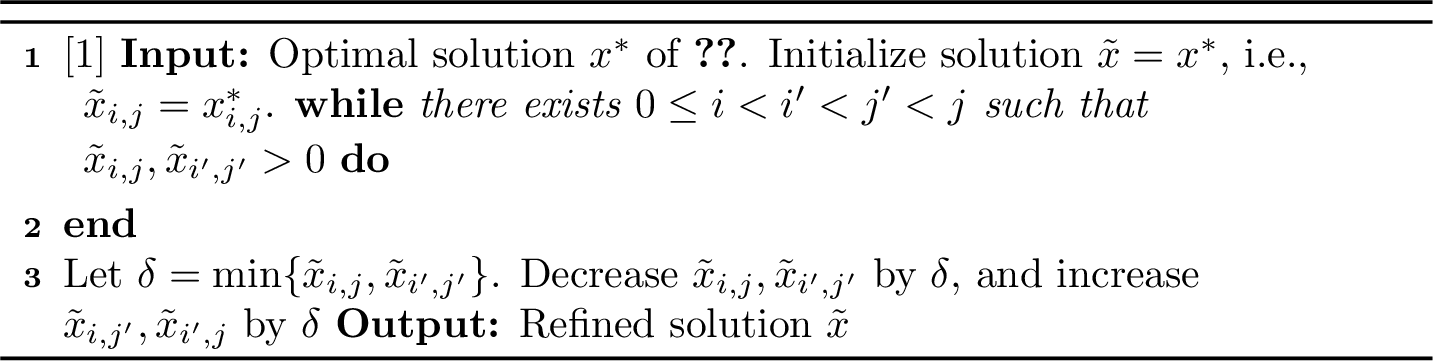
Intuitively, 1 ensures that the refined solution satisfies a "first buy first sell" policy: Since the bought (fractional) items are interchangable, for each step it sells first at request \(j'\) the item bought early at \(i\), and then sells the remaining ones at \(j\). The refined solution remains feasible and the objective is unchanged, which is formally proved in 11.
Claim 11. The output \(\tilde{x}\) of 1 is an optimal solution for 1 , i.e., \(\tilde{x}\) is feasible and it satisfies \({\mathsf{LP}}(\tilde{x}) = {\mathsf{LP}}(x^*)\).
Proof. It suffices to show that after performing one step of uncrossing in 1, the feasibility of \(\tilde{x}\) holds, and the objective remains unchanged. For the objective, note that the objective of 1 only depends on the value of every \(q^b_i(\tilde{x})\) and \(q^s_i(\tilde{x})\). Since the values of \(q^b_i(\tilde{x})\) and \(q^s_i(\tilde{x})\) remain unchanged after performing one uncrossing step, the objective remains unchanged. For Constraints 2 , it can be rewritten as \(q^b_i(\tilde{x}) + q^s_i(\tilde{x}) \leq p_i\), which remains feasible as every \(q^b_i(\tilde{x})\) and \(q^s_i(\tilde{x})\) remain unchanged. For Constraints 3 , it can be verified that for every \(t \in [T]\), the quantity \(\sum_{i = 0}^{t-1} \sum_{j = t}^T x_{i, j}\) is unchanged, so the constraint remains feasible. ◻
Next, we present the algorithm for decomposing the uncrossed optimal solution \(\tilde{x}\). We start from presenting an initial decomposition via 2.

2 provides an almost ready decomposition for solution \(\tilde{x}\). To be specific, we show the following 12:
Lemma 12. Assume the output \(\mathcal{I}\) of 2 equals to \(\{[\ell_1, r_1], \cdots [\ell_D, r_D]\}\), such that intervals are sorted in order, i.e., \(r_d + 1 = \ell_{d+1}\) for every \(d \in [D - 1]\). Then, the following statements hold when the input \(\tilde{x}\) of 2 is provided by 1:
For every \(d \in [D]\), we have \(\sum_{i = \ell_d}^{r_d} q^b_i(\tilde{x}) \leq 2.5\) and \(\sum_{i = \ell_d}^{r_d} q^s_i(\tilde{x}) \leq 2.5\).
For every \((i, j)\) that satisfies \(\tilde{x}_{i, j} > 0\) and \(i \neq 0\), \(i\) and \(j\) cross at most two adjacent intervals, i.e., assume \(i \in [\ell_d, r_d]\) and \(j \in [\ell_{d'}, r_{d'}]\), there must be \(d' \leq d + 1\).
Our proof of 12 relies on the following 13. At a high level, the claim follows the fact that for each interval \([l,r]\), \(\sum_{i = \ell}^r q^b_i(x) - \sum_{i = \ell}^r q^s_i(x)\) is the difference between total fractional items after request \(r\) and before request \(l\) w.r.t. the solution \(x\), whose absolute value must be at most 1 since the decision maker can hold at most one item.
Claim 13. Let \(x\) be a feasible solution of 1 . For every \(0 \leq \ell \leq r \leq T\), there must be \[\left|\sum_{i = \ell}^r q^b_i(x) - \sum_{i = \ell}^r q^s_i(x)\right| ~\leq ~ 1.\]
Proof. We prove via contradiction. Assume for interval \([\ell, r]\), we have \[\sum_{i = \ell}^r q^b_i(x) - \sum_{i = \ell}^r q^s_i(x) ~>~ 1.\] If \(r = T\), we may without loss of generality reduce \(r\) to \(T - 1\), as \(q^b_T(x)\) must be \(0\). When \(r \leq T - 1\), note that \[\begin{align} \sum_{i = 0}^r \sum_{j = r+1}^T x_{i, j} ~&\geq~ \sum_{i = \ell}^r \sum_{j = r+1}^T x_{i, j} \\ ~&=~ \sum_{i = \ell}^r q^b_i(x) - \sum_{i = \ell}^{r - 1} \sum_{j = i + 1}^r x_{i,j} \\ ~&\geq~ \sum_{i = \ell}^r q^b_i(x) - \sum_{i = \ell}^r q^s_i(x) ~>~ 1, \end{align}\] which is in contrast to the assumption that \(x\) is feasible as the constraint in the third line of 1 with \(t = r + 1\) is not satisfied. Therefore, there must be \(\sum_{i = \ell}^r q^b_i(x) - \sum_{i = \ell}^r q^s_i(x) ~\leq~ 1\).
Symmetrically, when \(\sum_{i = \ell}^r q^s_i(x) - \sum_{i = \ell}^r q^b_i(x) > 1\) holds, we may assume without loss of generality that \(\ell \geq 1\), as \(q^s_0(x)\) must be \(0\). Then, note that \[\begin{align} \sum_{i = 0}^{\ell - 1} \sum_{j = \ell}^T x_{i, j} ~&\geq~ \sum_{i = 0}^{\ell - 1} \sum_{j = \ell}^r x_{i, j} \\ ~&=~ \sum_{j = \ell}^r q^s_j(x) - \sum_{i = \ell}^{r - 1} \sum_{j = i + 1}^r x_{i, j} \\ ~&\geq~ \sum_{j = \ell}^r q^s_j(x) - \sum_{j = \ell}^r q^b_j(x) ~>~ 1, \end{align}\] which violates the constraint in the third line of 1 with \(t = \ell\). Combining two cases proves 13. ◻
Now, we are ready to prove 12.
Proof of 12. We first show 12.[item:init-decompose-i], i.e., within each interval \([\ell_d, r_d]\), the summation of \(q^b_i(\tilde{x})\) and \(q^s_i(\tilde{x})\) are both bounded by \(2.5\). Note that if the desired index \(r\) in Line 5 of 2 does not exist, then at least one summation must be bounded by \(1\), and 13 guarantees that another summation is bounded by 2, so 12.[item:init-decompose-i] holds. We then consider the general case where index \(r_d\) can be found. Since taking \(r_d - 1\) is not feasible, there must be \[\sum_{i = \ell_d}^{r_d - 1} q^b_i(\tilde{x}) ~<~ 1 \qquad \text{or} \qquad \sum_{i = \ell_d}^{r_d - 1} q^s_i(\tilde{x}) ~<~ 1.\] By 13, we have \[\begin{align} \sum_{i = \ell_d}^{r_d - 1} q^s_i(\tilde{x}) + \sum_{i = \ell_d}^{r_d - 1} q^b_i(\tilde{x}) ~&=~ \min\left\{ \sum_{i = \ell_d}^{r_d - 1} q^s_i(\tilde{x}), \sum_{i = \ell_d}^{r_d - 1} q^b_i(\tilde{x})\right\} + \max\left\{ \sum_{i = \ell_d}^{r_d - 1} q^s_i(\tilde{x}), \sum_{i = \ell_d}^{r_d - 1} q^b_i(\tilde{x})\right\} \\ ~&\leq~ 2 \cdot \min\left\{ \sum_{i = \ell_d}^{r_d - 1} q^s_i(\tilde{x}), \sum_{i = \ell_d}^{r_d - 1} q^b_i(\tilde{x})\right\} + 1 ~<~ 3. \end{align}\] Note that Constraint 2 guarantees \[q^s_{r_d}(\tilde{x}) + q^b_{r_d}(\tilde{x}) ~\leq~ p_{r_d} ~\leq~ 1.\] Summing the above two inequalities together gives \[\sum_{i = \ell_d}^{r_d} q^s_i(\tilde{x}) + \sum_{i = \ell_d}^{r_d} q^b_i(\tilde{x}) ~\leq~ 4.\] Since 13 guarantees that \[\left |\sum_{i = \ell_d}^{r_d} q^s_i(\tilde{x}) - \sum_{i = \ell_d}^{r_d} q^b_i(\tilde{x}) \right| ~\leq~ 1,\] there must be \[\sum_{i = \ell_d}^{r_d} q^b_i(\tilde{x}) ~\leq~ 2.5 \qquad \text{and} \qquad \sum_{i = \ell_d}^{r_d} q^s_i(\tilde{x}) ~\leq~ 2.5.\]
Next, we prove 12.[item:init-decompose-ii] via contradiction. Assume there exists \(1 \leq i' < j' \leq T\) that satisfies \(\tilde{x}_{i', j'} > 0\), such that \(d' - d \geq 2\) when \(i' \in [\ell_d, r_d]\) and \(j' \in [\ell_{d'}, r_{d'}]\). Consider \(j \in [\ell_{d+1}, r_{d+1}]\), and \(i \leq j\) that satisfies \(\tilde{x}_{i, j} > 0\). Recall that solution \(\tilde{x}\) is given by 1 after finishing the uncrossing process. Since we have \(j \leq r_{d+1} < \ell_{d'} \leq j'\), there must be \(i \leq i' \leq r_d < \ell_{d+1}\). Then, we have \[\begin{align} \sum_{i = 0}^{\ell_{d+1} - 1} \sum_{j = \ell_{d+1}}^T \tilde{x}_{i, j} ~&\geq~ \tilde{x}_{i', j'} + \sum_{i = 0}^{\ell_{d+1} - 1} \sum_{j = \ell_{d+1}}^{r_{d+1}} \tilde{x}_{i, j} \\ ~&=~ \tilde{x}_{i', j'} + \sum_{j = \ell_{d+1}}^{r_{d+1}} q^s_j(\tilde{x}) \\ ~&\geq~ \tilde{x}_{i', j'} + 1 > 1, \end{align}\] where the first inequality uses the fact that \(j' \notin [\ell_{d+1}, r_{d+1}]\), and therefore not counted in the following summation, the second equality uses the fact that \(\tilde{x}_{i, j} > 0\) for \(j \in [\ell_{d+1}, r_{d+1}]\) implies \(i < \ell_{d+1}\), and the last line uses the fact that 2 guarantees that \(\sum_{i = \ell_{d+1}}^{r_{d+1}} q^s_i(\tilde{x}) \geq 1\) (note that \(d+1 < d'\), so \(r_{d+1}\) can’t be \(T\)). Since the above inequality violates the constraint in the third line of 1 with \(t = \ell_{d+1}\), the assumption that \((i', j')\) exists is in contrast to the feasibility of solution \(\tilde{x}\). Therefore, 12.[item:init-decompose-ii] holds. ◻
Finally, we prove 10 by combining 11 and 12.
Proof of 10. To prove 10, we decompose solution \(\tilde{x}\) into three solutions \(\tilde{x}^{(1)}\), \(\tilde{x}^{(2)}\), and \(\tilde{x}^{(3)}\), such that these three solutions satisfy the first and second statements in 10. Then, we use 11, which states that \({\mathsf{LP}}(\tilde{x}) = {\mathsf{LP}}(x^*)\), to prove the third statement.
Constructing \(\tilde{x}^{(1)}\) and proof of 10.[item:decompose-opt-i]. We first give the definition of \(\tilde{x}^{(1)}\) and show that there exists an online algorithm achieving \(\frac{1}{2} \cdot {\mathsf{LP}}(\tilde{x}^{(1)})\). For \(0 \leq i < j \leq T\), we define \[\tilde{x}^{(1)}_{i, j} ~:=~ \tilde{x}_{i, j} \cdot \mathbf{1}[i = 0],\] i.e., \(\tilde{x}^{(1)}\) represents all trades that buys (for free) from request \(0\). Since solution \(\tilde{x}^{(1)}\) only buys from request \(0\) with at most one copy, the selling process given by \(\tilde{x}^{(1)}\) can be viewed as the LP solution of a single-item Prophet Inequality problem, and a standard Prophet Inequality algorithm achieves an expected profit of \(\frac{1}{2} \cdot {\mathsf{LP}}(\tilde{x}^{(1)})\). See e.g. [12] and its references for details.
Constructing \(\tilde{x}^{(2)}, \tilde{x}^{(3)}\) and proof of 10.[item:decompose-opt-ii]. Given \(\tilde{x}\), we run 2 to get the initial decomposition \(\mathcal{I}\) for \(\tilde{x}\), and we assume without loss of generality that \(\mathcal{I}= \{[\ell_1, r_1], \cdots [\ell_D, r_D]\}\), such that intervals are sorted in order, i.e., \(\ell_1 = 1, r_D = T\), and \(r_d + 1 = \ell_{d+1}\) for every \(d \in [D - 1]\). We define \(\tilde{x}^{(2)}\) and \(\tilde{x}^{(3)}\) as follows: \[\begin{align} \tilde{x}^{(2)}_{i, j} ~:=~ \tilde{x}_{i, j} \cdot \mathbf{1}\big[i \in [\ell_d, r_d]: d \text{ is odd}\big], \quad \text{and} \quad \tilde{x}^{(3)}_{i, j} ~:=~ \tilde{x}_{i, j} \cdot \mathbf{1}\big[i \in [\ell_d, r_d]: d \text{ is even}\big]. \end{align}\]
Now, we prove 10.[item:decompose-opt-ii]. We only prove the statement for \(\tilde{x}^{(2)}\), as the proof for \(\tilde{x}^{(3)}\) is identical. Define \(\mathcal{I}_{odd} = \{[\ell_d, r_d] \cup [\ell_{d+1}, r_{d+1}]: d \in [D]\land d \text{ is odd}\}\), where the last interval is refined as \([\ell_D, r_D]\) instead of \([\ell_D, r_D] \cup [\ell_{D+1}, r_{D+1}]\) when \(D\) is odd. Since 12 guarantees that for \((i, j): \tilde{x}_{i, j} > 0 \land i \in [\ell_d, r_d]\), there must be either \(j \in [\ell_d, r_d]\) or \(j \in [\ell_{d+1}, r_{d+1}]\) (if exists), for \((i, j): \tilde{x}^{(2)}_{i, j} > 0\), both \(i\) and \(j\) must belong to one interval in \(\mathcal{I}_{odd}\). Therefore, interval set \(\mathcal{I}_{odd}\) is a feasible decomposition of solution \(\tilde{x}^{(2)}\).
It remains to show that for each interval \([\ell, r] \in \mathcal{I}_{odd}\), solution \(\left\{\tilde{x}^{(2)}_{i, j} \cdot \mathbf{1}\big[i, j \in [\ell, r]\big]\right\}\) is a \(2.5\)-trades solution. Assume \(\ell\) equals to \(\ell_d\), where \(d\) is odd. By the definition of \(\tilde{x}^{(2)}\) and 12.[item:init-decompose-ii], solution \(\left\{\tilde{x}^{(2)}_{i, j} \cdot \mathbf{1}\big[i, j \in [\ell, r]\big]\right\}\) includes all trades of solution \(\tilde{x}\) that buys from a request within interval \([\ell_d, r_d]\), i.e., we have \[\begin{align} \sum_{i, j \in [\ell, r]^2} \tilde{x}^{(2)}_{i, j} \cdot \mathbf{1}\big[i, j \in [\ell, r]\big] ~=~ \sum_{i \in [\ell_d, r_d]} q^b_i(\tilde{x}) ~\leq~ 2.5, \end{align}\] where the inequality follows from 12.[item:init-decompose-i]. Therefore, \(\left\{\tilde{x}^{(2)}_{i, j} \cdot \mathbf{1}\big[i, j \in [\ell, r]\big]\right\}\) is a \(2.5\)-trades solution, and solution \(\tilde{x}^{(2)}\) admits a \(2.5\)-trades decomposition.
Proof of 10.[item:decompose-opt-ii]. We note that it suffices to show \(\tilde{x}^{(1)}+ \tilde{x}^{(2)}+ \tilde{x}^{(3)} = \tilde{x}\), as when the equality holds, we have \[{\mathsf{LP}}(\tilde{x}^{(1)}) + {\mathsf{LP}}(\tilde{x}^{(2)}) + {\mathsf{LP}}(\tilde{x}^{(3)}) ~=~ {\mathsf{LP}}(\tilde{x}) ~=~ {\mathsf{LP}}(x^*),\] where the last equality follows from 11. Note that for every \((i, j): \tilde{x}_{i, j} > 0\), we have \[\begin{align} \tilde{x}_{i, j} ~&=~ \tilde{x}_{i, j} \cdot \left(\mathbf{1}[i = 0] + \mathbf{1}[i \in [\ell_d, r_d]:d \text{ is odd}] + \mathbf{1}[i \in [\ell_d, r_d]:d \text{ is even}]\right) \\ ~&=~ \tilde{x}^{(1)}_{i, j} + \tilde{x}^{(2)}_{i, j} + \tilde{x}^{(3)}_{i, j}, \end{align}\] where the first equality holds since the conditions in three indicator functions partition all possibilities for tuple \((i, j)\). Therefore, equality \(\tilde{x}^{(1)}+ \tilde{x}^{(2)}+ \tilde{x}^{(3)} = \tilde{x}\) holds. ◻
3 Positive Results for Identical Request Distributions↩︎
In this section, we analyze the case with where the requests at each time are i.i.d.draws from some distribution \(\mathcal{D}\). This i.i.d. structure allows us to write a time-independent LP giving an upper bound on the optimal value; we then show a generic rounding algorithm whose performance is parameterized in terms of the expected number of sales made by the algorithm (see [thm:iid-large-general]). As a corollary of this result, we get the positive results stated in 3, 4, and 5.
3.1 A Stronger Benchmark and Linear-Programming Relaxation↩︎
To better exploit the assumption that all request are i.i.d.draws from the distribution \(\mathcal{D}\), we compare our online algorithms in this section to a stronger benchmark. Consider an offline algorithm with no capacity constraint for intermediate steps, i.e., the decision maker only needs to make sure that the final number of copies falls between \([0, B]\), but it may hold more than \(B\) or even fewer than \(0\) copies during intermediate steps; equivalently, this offline algorithm is allowed to exchange the order of all arriving requests to stay within the capacity bounds of \([0,B]\). Let such an offline algorithm be called an “order-independent algorithm”, and let the “order-independent profit” be the optimal profit achieved by such an order-independent algorithm. Since this is a relaxation, the optimal order-independent profit is at least the profit of the optimal offline algorithm with capacity constraints (which is not allowed to reorder requests). Furthermore, since the request are i.i.d., the optimal order-independent algorithm, performs the same operation on every request in expectation. Given this observation, we can further relax the optimal order-independent profit to a linear program: assume the distribution \(\mathcal{D}\) has support size \(K\), such that the distribution \(\mathcal{D}\) generates price tuple \((b^{(k)}, s^{(k)})\) with probability \(p^{(k)}\), for \(k \in [K]\). Our LP relaxation is:
\[\begin{align} {2} \text{maximize} \qquad T \cdot \sum_{k \in [K]} \big(s^{(k)} \cdot y_k &- b^{(k)} \cdot z_k \big) && _{\mathrm{\small IID}}} \tag{6} \\ \text{s.t.}\quad y_k + z_k &\leq p^{(k)} &\qquad& \forall k \in [K], \tag{7} \\ B_0 + T \cdot \sum_{k \in [K]} (z_k - y_k) &\in [0, B] && \forall t \in [T],\tag{8} \\ y_k, z_k &\geq 0. && \notag \end{align}\]
Intuitively, the LP variables \(y_k\) and \(z_k\) represent the probability of an order-independent algorithm selling or buying a copy, when the type of a request is \(k\). Constraints 7 ensure that the probability of buying or selling when the type is \(k\) cannot exceed \(p^{(k)}\); constraints 8 ensure that the algorithm holds at most \(B\) copies and at least \(0\) copy when the process ends.
Let \((y^*, z^*)\) be the optimal solution to 6 . Define \[\begin{align} \alpha_B~:=~ \sum_{k \in [K]} z^*_k \qquad \text{and} \qquad \alpha_S~:=~ \sum_{k \in [K]} y^*_k \label{eq:iid-bsprob-balance} \end{align}\tag{9}\] to be the expected number of copies we buy and sell at each step. Without loss of generality, we assume that for solution \((y^*, z^*)\), constraint 8 achieves its lower bound, i.e., \[\begin{gather} B_0 + T \cdot \sum_{k \in [K]} (z^*_k - y^*_k) ~=~ B_0 + T \cdot (\alpha_B- \alpha_S) ~=~0, \label{eq:1} \end{gather}\tag{10}\] as otherwise we can either find some \(z^*_k > 0\) such that decreasing the value of \(z^*_k\) increases the objective function, or such \(z^*_k\) does not exist and the instance becomes trivial where we always sell during the whole process. This observation further implies that the optimal solution \((y^*, z^*)\) is not constrained by the upper bound \(B\) in 8 .
We further define \[\begin{align} \Gamma ~:=~ T \cdot \alpha_S~=~ B_0 + T \cdot \alpha_B\label{eq:iid-gamma-def} \end{align}\tag{11}\] to be the expected number of copies we sell during the whole process.
If \({\mathsf{LP}}(y, z)\) is the objective value of 6 corresponding to a feasible solution \((y, z)\), the following lemma shows that \({\mathsf{LP}}(y, z)\) is at least the expected profit of an optimal offline algorithm to the ATP problem in the i.i.d.case.
Lemma 14 (Relaxation). The linear program 6 is a relaxation of the ATP problem for i.i.d.requests. In other words, let \((y^*, z^*)\) be the optimal solution to 6 , then \({\mathsf{LP}}(y^*, z^*)\) is at least the expected profit of the optimal offline algorithm for the ATP problem.
Proof. Consider the structure of the optimal order-independent algorithm. Since the decision of such algorithm does not depend on the arrival order of requests, while every request is identically distributed, in expectation the optimal decision of the algorithm should only depend on the type of each request, rather than the order of their arrivals. Given this observation, we define without loss of generality \(\tilde{y}_k\) to be the probability that the arriving request has type \(k\) and the optimal order-independent algorithm buys at price \(b^{(k)}\), and define \(\tilde{z}_k\) to be the probability that the arriving request has type \(k\) and the optimal order-independent algorithm sells at price \(s^{(k)}\). Then, there must be \(b^{(k)} + s^{(k)} \leq p^{(k)}\), as \(p^{(k)}\) is the probability that type \(k\) is realized. The inequality \[B_0 + T \cdot \sum_{k \in [K]} \tilde{z}_k - \tilde{y}_k ~\in [0, B]\] also holds, as the LHS represents the expected final inventory of the optimal order-independent algorithm. Then, \((\tilde{y}, \tilde{z})\) is a feasible solution of 6 , and therefore \({\mathsf{LP}}(y^*, z^*)\) upper-bounds the expected profit of the optimal offline algorithm, as we have \({\mathsf{LP}}(y^*, z^*) \geq {\mathsf{LP}}(\tilde{y}, \tilde{z})\), while the optimal order-independent profit upper-bounds the expected profit of the optimal offline algorithm. ◻
Given 14, it suffices to provide an online algorithm with an expected profit comparable to \({\mathsf{LP}}(y^*, z^*)\).
3.2 A Unified Algorithm for Large Capacity↩︎
In this subsection, we prove the results for the setting where capacity \(B\) is sufficiently large. Our main technical theorem is [thm:iid-large-general]; we later derive our results for both the the symmetric case (where \(b_t = s_t\) for all \(t\)) and the asymmetric case from this theorem.
Consider 3 which performs a natural randomized rounding, with one important change: as we approach the end of the online process, we implement a sell-only strategy to clear the remaining inventory to the extent possible. This sell-only stage is necessary, as the benchmark \({\mathsf{LP}}(y^*, z^*)\) decomposes into two parts: the revenue from selling the initial inventory \(B_0\), and the trading profit earned from \(T\) requests. As the revenue from either part can be arbitrarily larger than the other, we ensure that 3 tries to clear its inventory when it ends.

Theoremiidmain Given an ATP instance with i.i.d.requests, 3 achieves a competitive ratio of \(1 - O(\log B \cdot \Gamma^{-1/2} + B^{-1})\) against the optimal objective of 6 , provided \(B_0 \geq 1\).
We defer the somewhat technical proof of [thm:iid-large-general] to 8; here is a high-level idea of the proof. Under the assumption that 3 clears all the inventory, its performance depends on the number of blocked trades, i.e., buys that cannot happen when the inventory equals \(B\), and the sales that are blocked because the inventory reaches \(0\). We show that when \(\Gamma\) is much smaller than \(B^2\), since the standard deviation of the whole trading process is \(O(\sqrt{\Gamma})\), and hence the number of blocked trades is bounded by \(O(\sqrt{\Gamma})\); on the other hand, when \(\Gamma\) is much larger than \(B^2\), the trading process tends to stabilize, allowing us to show that the inventory level at each timestep is close to being uniformly distributed over \([0, B]\). In turn, this means that an \(O(B^{-1})\) fraction of trades are blocked in expectation. Combining these two cases proves [thm:iid-large-general]. While we defer the full proof to the appendix, we now derive our results for the i.i.d.case from it in the next subsections.
3.3 Positive Results for the Large Capacity Case↩︎
We first use [thm:iid-large-general] to prove our positive results in 4 and 5 for the case of large budgets; the corresponding lower bounds of these will be proved in 4.
Proof of 5[item:asym-large-ub] and 4[item:sym-large-ub]. To prove the competitive ratio for the asymmetric case, we apply 3 with an extra pre-processing step: given an ATP instance with i.i.d. requests, we first solve 6 with the original capacity upper bound \(B\), but run 3 with a reduced capacity upper bound \(B_0\). This pre-processing step is feasible, as we recall that the optimal solution \((y^*, z^*)\) of 6 is not constrained by the upper bound \(B\) in constraint 8 . Since \(\Gamma = B_0 + T \cdot \alpha_B\geq B_0\), 3 achieves at least \(1 - O(\frac{\log B_0}{\sqrt{B_0}})\) times the \({\mathsf{LP}}(y^*, z^*)\), and therefore the competitive ratio of 3 is \(1 - O(\frac{\log B}{\sqrt{B_0}})\).
To prove the stronger bound of \(1 - O(\frac{(\log B)}{\sqrt{B}})\) for the symmetric case where \(b^{(k)} = s^{(k)}\), our proof relies on the following observation: given an ATP instance with symmetric prices, let \((y^*, z^*)\) be the optimal solution of 6 . If \(y^*_k + z^*_k < p^{(k)}\) for some \(k \in [K]\), increase \(y^*_k\) and \(z^*_k\) equally until constraint 7 becomes tight; note that the constraint 8 and the objective function value remain unchanged. Therefore, without loss of generality we may assume that constraint 7 is tight, and therefore \[\alpha_S+ \alpha_B~=~ \sum_{k \in [K]} (y^*_k + z^*_k) ~=~ \sum_{k \in [K]} p^{(k)} ~=~ 1,\] which implies \[2\Gamma ~=~ B_0 + T \cdot (\alpha_S+ \alpha_B) ~=~ B_0 + T ~\geq~ B;\] the final inequality uses the assumption from 1.1 that \(B \leq B_0+T\). Therefore, the competitive ratio of 3 for the ATP problem with symmetric prices becomes \(1 - O(\frac{\log B}{\sqrt{B}})\). ◻
3.4 Positive Results for the Unit Capacity Case↩︎
We now prove 3, our result for the ATP problem with i.i.d.requests. Given an ATP instance with request distribution \(\mathcal{D}\), having unit capacity \(B\) and unit initial inventory level \(B_0\), let \((y^*, z^*)\) be the optimal solution of 6 . To begin, observe that (10 ) implies that \[T \cdot \sum_k y^*_k = T\cdot \alpha_S\geq B_0 = 1.\] Now define two solutions to (6 ): \[\begin{align} {2} y'_k &= y^*_k/(T\alpha_S) & \qquad\text{and}\qquad & z'_k = 0, \\ y''_k &= y^*_k - y'_k &\qquad\text{and}\qquad & z''_k = z^*_k. \label{eq:balanced-solution} \end{align}\tag{12}\]
Lemma 15. The solutions \((y', z')\) and \((y'', z'')\) are both feasible solutions of 6 .
Proof. Since \(T\alpha_S\geq 1\), we have that \(y'_k \in [0, y^*_k]\) and hence \(y''_k \leq y^*_k\). Therefore both the non-negativity constraints and constraint (7 ) are satisfied for both solutions. To verify (8 ) for \((y', z')\), note that \(B_0 + T \sum_k (z'_k - y'_k) = B_0 - \sum_k y'_k = B - 1 = 0\). Finally, \(B_0 + T \sum_k (z''_k - y''_k) = B_0 + T(\alpha_B- \alpha_S) + 1 = 0 + 1 \leq B\), where we used the definition of \((y'',z'')\) for the first equality, and (10 ) for the second equality. ◻
15 shows the feasibility of \((y', z')\) and \((y'', z'')\). We now give rounding algorithms for the two solutions \((y', z')\) and \((y'', z'')\). For solution \((y', z')\), we show in 16 that an independent rounding algorithm recovers a constant fraction of \({\mathsf{LP}}(y', z')\).
Lemma 16. There exists an algorithm that rounds solution \((y', z')\) to get an expected profit of \(\frac{1}{2} \cdot {\mathsf{LP}}(y', z')\).
Proof. Observe that the fractional process corresponding to \((y', z')\) performs no buying action, and the total number of (fractional) selling action is \(1\). Therefore, solution \((y', z')\) can be viewed as the LP relaxation of a single-item Prophet Inequality instance. To be specific, consider the following independent rounding algorithm: when price tuple \((b_t, s_t)\) is realized with type \(k\), i.e., \((b_t, s_t) = (b^{(k)}, s^{(k)})\), we sell the unit inventory at price \(s^{(k)}\) with probability \(\frac{y'_k}{p^{(k)}}\), and terminate the process once this only copy is sold. Then, given that the inventory is not sold before \((b_t, s_t)\) is revealed, the probability that the inventory get sold is exactly \[\sum_{k \in [K]} p^{(k)} \cdot \frac{y'_k}{p^{(k)}} ~=~ \sum_{k \in [K]} p^{(k)} ~=~ \frac{\sum_{k\in [K]} y^*_k}{T \cdot \alpha_S} ~=~ T^{-1},\] and therefore the inventory remains unsold during the whole process is at least \[\left( 1 - \frac{1}{T} \right)^T ~\leq~ \frac{1}{e}.\] Therefore, the expected profit from this independent rounding process is at least \[\left(1 - \frac{1}{e}\right) \cdot \frac{\sum_{k \in [K]} p^{(k)} \cdot \frac{y'_k}{p^{(k)}} \cdot s^{(k)}}{T^{-1}} ~=~ \left(1 - \frac{1}{e}\right) \cdot {\mathsf{LP}}(y', z') ~\geq~ \frac{1}{2} \cdot {\mathsf{LP}}(y', z').\] where the equality follows from the fact that \(z'_k = 0\) for every \(k \in [K]\). ◻
To round the solution \((y'',z'')\), we give the following 4.
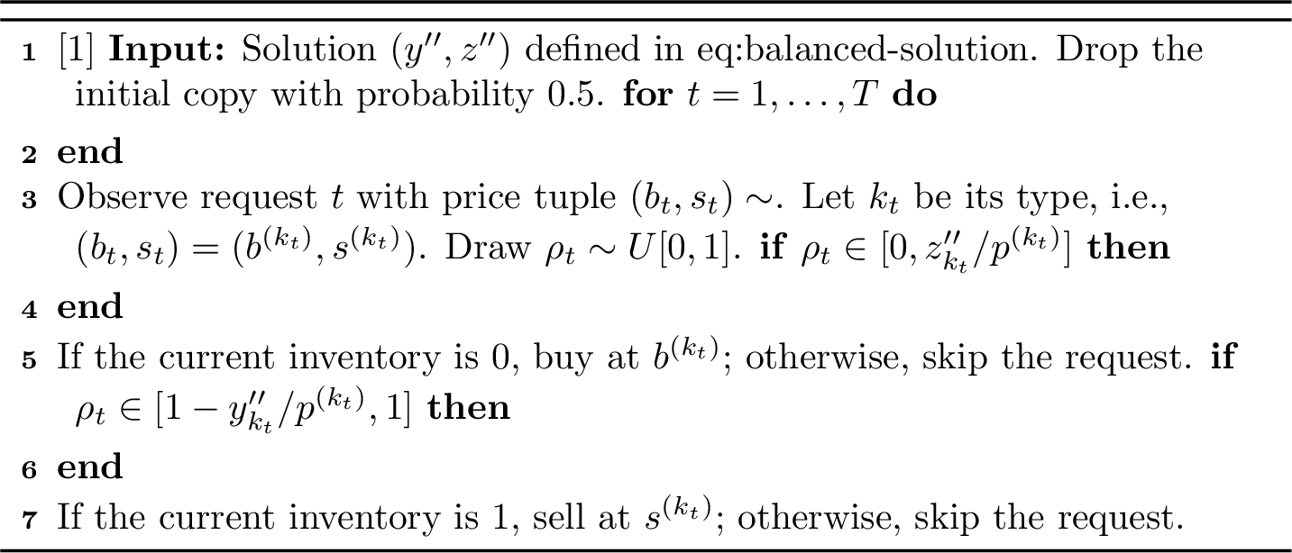
Lemma 17. 4 gets an expected profit of \(\frac{1}{2} \cdot{\mathsf{LP}}(y'', z'')\).
Proof. Our proof relies on the following key observation: note that \[\begin{align} \sum_{k \in [K]} y''_k ~=~ \sum_{k \in [K]} y^{*}_k - \sum_{k \in [K]} y'_k ~=~ \alpha_S- \frac{B_0}{T} ~=~ \frac{\Gamma - B_0}{T} ~=~ \alpha_B~=~ \sum_{k \in [K]} z''_k, \end{align}\] i.e., regarding each request, following solution \((y'', z'')\) leads to the same probability of buying or selling a copy. Then, the probability that the inventory is \(0\) (or \(1\)) before every request \(t \in [T]\) arrives must be \(0.5\).
We prove the above statement via induction. The base case is \(t = 1\). The statement holds as we drop the initial copy with probability \(0.5\). Now assume \(\mathbf{Pr}[\text{inventory is }0 \text{ before }t] = 0.5\). For request \(t\), we have \[\begin{align} \mathbf{Pr}[\text{inventory is }0 \text{ before }t + 1] ~=~& \mathbf{Pr}[\text{inventory is }0 \text{ before }t] \cdot \Big(1 - \sum_{k \in [K]} p^{(k)} \cdot \frac{z''_k}{p^{(k)}} \Big) \\ ~&+ \mathbf{Pr}[\text{inventory is }1 \text{ before }t] \cdot \sum_{k \in [K]} p^{(k)} \cdot \frac{y''_k}{p^{(k)}} \\ ~=~& \frac{1}{2} \Big(1 - \sum_{k \in [K]} z''_k + \sum_{k \in [K]} y''_k \Big) ~=~ 0.5. \end{align}\] Therefore, \(\mathbf{Pr}[\text{inventory is }0 \text{ before }t + 1] = 0.5\) also holds, which implies the probability that the inventory is \(0\) (or \(1\)) before every request \(t \in [T]\) arrives is \(0.5\). Then, by linearity of expectation, the expected profit of 4 is \[\begin{align} &\sum_{t \in [T]} \sum_{k \in [K]} p^{(k)} \cdot \frac{y''_k}{p^{(k)}} \cdot s^{(k)} \cdot \mathbf{Pr}[\text{inventory is }1 \text{ before }t] \\ &~~- \sum_{t \in [T]} \sum_{k \in [K]} p^{(k)} \cdot \frac{z''_k}{p^{(k)}} \cdot b^{(k)} \cdot \mathbf{Pr}[\text{inventory is }0 \text{ before }t] \\ ~=~& \frac{T}{2} \cdot \Big(\sum_{k \in [K]} y''_k \cdot s^{(k)} - \sum_{k \in [K]} z''_k \cdot b^{(k)} \Big) ~=~ \frac{1}{2}\cdot {\mathsf{LP}}(y''_k, z''_k). \qedhere \end{align}\] ◻
Finally, combining 15, 16, and 17 together proves 3.
Proof of 3. Running the algorithm from 16 with probability \(\frac{1}{2}\), and 4 otherwise, gives an expected profit of \[\frac{1}{2} \cdot \frac{1}{2} \cdot {\mathsf{LP}}(y'_k, z'_k) + \frac{1}{2} \cdot \frac{1}{2} \cdot {\mathsf{LP}}(y''_k, z''_k) ~=~ \frac{1}{4} \cdot {\mathsf{LP}}(y^*, z^*),\] where the equality uses the fact that \(y^*_k = y'_k + y''_k\) and \(z^*_k = z'_k + z''_k\) for every \(k \in [K]\). ◻
4 Negative Results for the ATP Problem↩︎
In this section, we prove the hardness results for the ATP problem. We start with 1, which states that no competitiveness is achievable with no initial inventory, i.e., with \(B_0 = 0\).
Proof of 1. Consider an ATP instance with \(B_0 = 0\) and \(T = B\), where requests are i.i.d.draws from the following distribution \(\mathcal{D}\): \[\begin{align} (b, s) \sim D = \begin{cases} (1, 0) & \text{w.p. } 1 - \frac{0.1}{B} \\ (+\infty, 2) & \frac{0.1}{B} \\ \end{cases} \end{align}\] Note that if an online algorithm observes a price tuple \((1, 0)\) and decides to buy at price \(1\), the probability that it can sell at price \(2\) in the future is at most \[1 - \Big(1 - \frac{0.1}{B}\Big)^T ~\approx 1 - e^{-0.1} ~\leq~ 0.1.\] This suggests that an online algorithm should never buy at price \(1\), since the expected profit is at most \(-1 + 2 \cdot 0.1 < 0\); consequently, the optimal online algorithm has an expected profit of \(0\). However, an optimal offline algorithm, which can see the future, can check if there is a price tuple \((+\infty, 2)\) following some occurrence of \((1,0)\)—which happens with constant probability—and get unit profit in these scenarios. This implies that no online algorithm can have finite competitiveness with the offline optimum. ◻
Proof of 4[item:asym-large-lb]. For the negative result in 4, note that when we have \(b^{(k)} = +\infty\) for every price tuple \((b^{(k)}, s^{(k)})\) in the support of the identical request distribution \(\mathcal{D}\), the ATP problem degenerates to the \(B_0\)-unit Prophet Inequality problem with identical value distributions, leading to a \(1 - \Omega(1/\sqrt{B_0})\) lower bound (see [9]). ◻
4.1 The Negative Result for Symmetric Prices↩︎
Recall that we now need to prove 5[item:sym-large-lb], i.e., to bound the performance of any online algorithm for the setting where the prices are symmetric (i.e., \(b_t = s_t)\)) and the requests are i.i.d.draws from some distribution \(\mathcal{D}\).
Consider the following symmetric ATP instance with \(B = 1.5T = 3B_0\) for some large enough initial inventory level \(B_0\); observe that we can ignore the capacity bound \(B\), because \(B = B_0 + T\). (We assume \(T\) is suitably large for the lower bound.) The underlying distribution \(\mathcal{D}\) is defined as follows: \[\begin{align} (b, s) \sim D = \begin{cases} (1, 1) & \text{w.p. } 0.75 \\ (0, 0) & \text{w.p. } 0.25 - 1/\sqrt{B} \\ (0.5, 0.5) & \text{w.p. } 1/\sqrt{B} \end{cases} \end{align}\] The strategy that buys items at price \(0\) and sells at \(1\) (whenever possible) makes \(\Omega(B)\) profit, and this is trivially the best possible. Therefore, to show that the competitive ratio of any online algorithm is at most \(1 - \Omega(1/\sqrt{B})\), it suffices to show that any online algorithm incurs at least an \(\Omega(\sqrt{B})\) (additive) regret against some offline algorithm—i.e., to show that for any online algorithm, there exists an offline algorithm achieving an expected profit of \(\Omega(\sqrt{B})\) more than the online algorithm.
For the proof, we define three events, which we show happen with constant probability each. For constants \(c_2 \ll c_1 \ll 1\), the two events are as follows:
Event \(\mathcal{E}_0\): The number of occurrences of each price \(0, \frac{1}{2}, 1\) in the time interval \([1,T/2]\) deviates from its expectation by at most \(c_1\, \sqrt{B}\).
Event \(\mathcal{E}_1\): The number of occurrences of the “low” prices \(0, \frac{1}{2}\) during \([T/2+1, T]\) is low enough that following the strategy (at all times in \([1,T]\)) of buying when a price \(0\) or \(\frac{1}{2}\) arrives, and selling when the price \(1\) arrives, ensures that the inventory never becomes negative at any moment, and that the final inventory level is in \([0.5c_2 \, \sqrt{B}, c_2 \, \sqrt{B}]\).
Event \(\mathcal{E}_2\): The number of occurrences of price \(0\) during \([T/2+1, T]\) is high enough that following the strategy (at all times \(T\)) of buying when \(0\) arrives, while selling when price \(1\) arrives, ensures that the inventory never becomes negative at any moment, and that the final inventory is again in \([0.5c_2 \, \sqrt{B}, c_2 \, \sqrt{B}]\).
Claim 18. The two events \(\mathcal{F}_1 := (\mathcal{E}_0 \cap \mathcal{E}_1)\) and \(\mathcal{F}_2 := (\mathcal{E}_0 \cap \mathcal{E}_2)\) happen with at least some absolute constant probability. Moreover, these events \(\mathcal{F}_1, \mathcal{F}_2\) are disjoint.
Proof. We give the proof for event \(\mathcal{F}_1\); the proof for \(\mathcal{F}_2\) is similar. The probability of \(\mathcal{E}_0\) is easy to analyze: standard Chernoff bounds ensure that the number of occurrences of each of the tuples deviates by more than \(c_1 \sqrt{B}\) is at most some constant. So it remains to bound the probability of \(\mathcal{E}_1\) given \(\mathcal{E}_0\). Fix the realization of the first half. Let \(B_t\) be the inventory after request \(t\) is processed, assuming we follow the strategy of selling a copy whenever the price equals \(1\), and buying a copy at all other “low” prices. Recall that \(\mathcal{E}_1\) requires two conditions:
Final Inventory Constraint: The final inventory \(B_T\) lands in \([0.5 c_2 \sqrt{B}, c_2 \sqrt{B}]\).
Intermediate Constraint: \(B_t \ge 0\) for all \(t \in (T/2, T]\).
Conditioned on the starting inventory \(B_{T/2}\), the Final Inventory Constraint requires the final inventory to be off by its expectation by \([c'\cdot \sqrt{B}, c'' \cdot \sqrt{B}]\) for some constants \(c', c''\) satisfying \(c'' - c' = 0.5\cdot c_2\). By a Chernoff bound, this happens with at least a constant probability.
Next, we take the Intermediate Constraint into consideration. We show that the probability that the Final Inventory Constraint holds while the Intermediate Constraint breaks is small enough. Note that if we follow the strategy of selling a copy whenever the price is \(1\) and buying a copy otherwise, in expectation the inventory decreases by \(0.5\) after processing each request. Therefore, when the Final Inventory Constraint holds while the Intermediate Constraint breaks, it indicates that within at most \(T\) steps after first hitting \(B_t = 0\), this random walk process, which has a constant leftward drift in expectation, travels \(0.5 c_2 \cdot \sqrt{B}\) steps to the right. Then, a standard random walk analysis can show that this event happens with probability at most \(e^{-\Omega(\sqrt{B})}\). Therefore, when the realization of the first half is fixed, we have \[\begin{align} &\mathbf{Pr}[\text{Final Inventory OK}\land \text{Intermediate OK}] \\ =~& \mathbf{Pr}[\text{Final Inventory OK}] - \mathbf{Pr}[\text{Final Inventory OK} \land \lnot \text{Intermediate OK}] \\ \geq~&\text{constant} \end{align}\] Finally, since the realizations of the two halves of the instance are independent, \(\mathbf{Pr}[\mathcal{E}_1]\) is at least an absolute constant. Furthermore, an identical analysis can also show that \(\mathbf{Pr}[\mathcal{F}_2]\) is at least an absolute constant. ◻
Proof of 5. Given the symmetric \({\textsf{ATP}}\) instance above. Now, given any online algorithm, we construct the following offline benchmark. When event \(\mathcal{F}_1\) happens, the offline algorithm simply buys whenever the price is \(0\) or \(0.5\), and sells whenever the price is \(1\). Similarly, when the disjoint event \(\mathcal{F}_2\) occurs, the offline algorithm buys whenever the price is \(0\) and sells whenever the price is \(1\). Otherwise, for all outcomes outside \(\mathcal{F}_1 \cup \mathcal{F}_2\), we mimic the online algorithm. It suffices to show that the offline algorithm significantly outperforms the online algorithm on at least one of these events.
We now analyze the performance loss of the online algorithm in these two cases. Observe that at time \(T/2\), the online algorithm cannot distinguish, conditioned on satifying \(\mathcal{E}_0\), whether the realization satisfies \(\mathcal{F}_1\) or \(\mathcal{F}_2\)—indeed, given the initial inventory level of \(B_0\) and the fact that \(T = 2B_0\), even selling at every single timestep would not cause inventory levels to be negative at time \(T/2\). Moreover, given \(\mathcal{E}_0\), the number of timesteps with price \(\frac{1}{2}\) is at least \[K := [(T/2) \cdot (1/\sqrt{B})] - c_1 \sqrt{B} = (1/3 - c_1)\cdot \sqrt{B}.\] We now consider whether the online algorithm purchases at least \(K/2\) copies at price \(\frac{1}{2}\) by \(T/2\).
If it does buy at least \(K/2\) copies at price \(\frac{1}{2}\), then its profit is less than the profit of the offline algorithm which only buys at 0 by at least \(K/2\), for all outcomes in \(\mathcal{E}_2\).
On the other hand, if the online algorithm purchases fewer than \(K/2\) copies at price \(\frac{1}{2}\) by time \(T/2\), then it must have rejected at least \(K/2\) copies at price \(\frac{1}{2}\). Now the algorithm that buys all items at prices \(0\) and \(\frac{1}{2}\) on outcomes in \(\mathcal{E}_1\) would buy all \(K\) these copies, and still sell them, thereby making at least \(K/2\cdot \frac{1}{2}\) more profit.
Since \(c_2, c_1 \ll 1\), this implies the regret of the online algorithm (versus an offline algorithm) is at least \(\Omega(\sqrt{B}) \cdot \min(\mathbf{Pr}[\mathcal{F}_1], \mathbf{Pr}[\mathcal{F}_2])\), which is \(\Omega(\sqrt{B})\) by 18, thereby completing the proof. ◻
5 Concentration Inequalities↩︎
The following two concentration inequalities, for independent random variables, and for martingales, will be used repeatedly in our analyses.
Theorem 19 (Bernstein’s Inequality). Let \(X_1, \ldots, X_N\) be independent mean-zero random variables such that \(|X_i| \leq R\) for all \(i\). Let \(\sigma^2 := \sum_{i \in [N]} \mathbb{E}[X^2_i]\) be the variance of \(\sum_{i \in [N]} X_i\). Then, for any \(\epsilon \geq 0\), we have \[\begin{align} \mathbf{Pr}\left(\sum_{i = 1}^N X_i \geq \epsilon \right) ~&\leq~ \exp\left(- \frac{\epsilon^2/2}{\sigma^2 + R\epsilon/3}\right) \quad \text{and} \\ \mathbf{Pr}\left(\sum_{i = 1}^N X_i \leq -\epsilon \right) ~&\leq~ \exp\left(- \frac{\epsilon^2/2}{\sigma^2 + R\epsilon/3}\right) \enspace . \end{align}\]
Theorem 20 (Freedman’s Inequality). Let \(\{Y_k\}_{k \ge 0}\) be a martingale with increments \(\Delta Y_k = Y_k - Y_{k-1}\) satisfying \(|\Delta Y_k| \le R\). Let \(\langle Y \rangle_n = \sum_{k=1}^n \mathbb{E}[X_k^2 \mid \mathcal{F}_{k-1}]\) be the predictable quadratic variation. Then for any \(\epsilon > 0\) and \(v > 0\): \[\mathbf{Pr}\left[ \max_{1 \le k \le n} |Y_k| \ge \epsilon \text{ and } \langle Y \rangle_n \le v \right] ~\le~ 2 \exp\left( -\frac{\epsilon^2 / 2}{v + R\epsilon / 3} \right) . \notag\]
6 Omitted Proofs in 2↩︎
In this section, we complete the missing proofs in 2.
6.1 Proof of Relaxation Lemma↩︎
Proof of 6. It suffices to show that taking \[x_{i, j} ~=~ \mathbf{Pr}\left[\text{optimal offline solution buys from }i \text{ and sells to }j\right]\] gives a feasible solution of 1 .
Constraints 2 are feasible, as the probability that the optimal offline algorithm chooses an action of either buy or sell for request \(i\) is at most \(p_i\). Constraints 3 are feasible, as the quantity of \(\sum_{i = 0}^{t-1} \sum_{j = t}^T x_{i, j}\) represents the expected number of the copy that the optimal offline algorithm carries after request \(t\), which is at most \(1\), as the offline algorithm can carry at most one copy at any time. Therefore, solution \(x\) is feasible. ◻
6.2 Proof of the \(m\)-Trades Lemma↩︎
Proof of 8. Note that it suffices to prove 8 only for \(m = 1\), since when solution \(x\) of 1 is an \(m\)-trades solution, \(x/m\) becomes a \(1\)-trade solution, and applying 8 to solution \(x/m\) gives the desired argument for \(x\).
When solution \(x\) is a \(1\)-trade solution on interval \([\ell, r]\), there must be \(\sum_{i = \ell}^r q^b_i(x) = \sum_{i = \ell}^r q^s_i(x) \leq 1\) (7.[item:mtrades-ii]), and the value of \(q^b_i(x)\) and \(q^s_i(x)\) can be non-zero only when \(i \in [\ell, r]\) (7.[item:mtrades-i]). Our main idea is to apply a standard OCRS algorithm based on the values \(q^b_i(x)\) and \(q^s_i(x)\). To be specific, we show that 5 is the desired algorithm for 8.

Proving the probability of holding a copy. We first prove that after 5 is finished, the algorithm still keeps a copy in hand with probability \(0.5\). To achieve this, we show that when the algorithm holds a copy when 5 begins, the copy is sold by 5 with probability \(\frac{1}{2} \cdot \sum_{i = \ell}^r q^s_i(x)\). We prove by induction that for each \(i\in [l, r]\), after request \(i\) arrives, the copy remains available with probability \(1 - \frac{1}{2} \cdot \sum_{j = \ell}^i q^s_j(x)\). The base case is \(i = \ell - 1\), and the copy is available with probability \(1\). Now assume the claim holds till request \(i-1\). If the item remains available for request \(i\), 5 sells the item with probability \[p_i \cdot \frac{q^s_i(x)}{p_i} \cdot \frac{0.5}{1 - 0.5 \cdot \sum_{j = \ell}^{i-1} q^s_j(x)} ~=~ \frac{0.5\cdot q^s_i(x)}{1 - 0.5 \cdot \sum_{j = \ell}^{i-1} q^s_j(x)}.\] Since whether the price tuple \((b_i, s_i)\) arrives and whether 5 sells the copy is independent to the decisions before request \(i\), the copy remains available after request \(i\) with probability \[\left(1 - \frac{1}{2} \cdot \sum_{j = \ell}^{i-1} q^s_j(x) \right) \cdot \left( 1 - \frac{0.5\cdot q^s_i(x)}{1 - 0.5 \cdot \sum_{j = \ell}^{i-1} q^s_j(x)} \right) ~=~ 1 - \frac{1}{2} \cdot \sum_{j = \ell}^{i} q^s_j(x),\] which proves the claim for the case after request \(i\). Then, applying the claim for request \(r\) shows that the item remains available with probability \(1 - \frac{1}{2} \cdot \sum_{i = \ell}^r q^s_i(x)\), and equivalently the item is sold with probability \(\frac{1}{2} \cdot \sum_{i = \ell}^r q^s_i(x)\).
Symmetrically, when the algorithm does not hold a copy when 5 begins, it buys a copy with probability \(\frac{1}{2} \cdot \sum_{i = \ell}^r q^b_i(x)\). Then, after 5 finishes, the algorithm holds a copy with probability \[0.5 \cdot \left(1 - \frac{1}{2} \cdot \sum_{i = \ell}^r q^s_i(x)\right) + 0.5 \cdot \frac{1}{2} \cdot \sum_{i = \ell}^r q^b_i(x) ~=~ 0.5,\] where we use the fact that \(\sum_{i = \ell}^r q^s_i(x) = \sum_{i = \ell}^r q^b_i(x)\) in the last equality, which is true because every non-zero \(x_{i,j}\) (buy at \(i\), sell at \(j\)) satisfies \(l\leq i<j\leq r\). So the total probability of buys and sells within the internal \([l,r]\) are equal.
Proving the expected profit. Next, we calculate the expected profit achieved by 5. We first calculate the expected selling gain. Recall that an item remains available for request \(i\) with probability \(1 - \frac{1}{2} \cdot \sum_{j = \ell}^{i-1} q^s_j(x)\), and the algorithm sells the item at price \(s_i\) with probability \(\frac{0.5\cdot q^s_i(x)}{1 - 0.5 \cdot \sum_{j = \ell}^{i-1} q^s_j(x)}\). Therefore, the total expected gain (assuming the algorithm holds a copy) is \[\begin{align} \sum_{i = \ell}^r s_i \cdot \frac{0.5\cdot q^s_i(x)}{1 - 0.5 \cdot \sum_{j = \ell}^{i-1} q^s_j(x)} \cdot \left(1 - \frac{1}{2} \cdot \sum_{j = \ell}^{i-1} q^s_j(x)\right) ~=~ \frac{1}{2} \cdot \sum_{i = \ell}^r s_i \cdot q^s_j(x). \end{align}\] Symmetrically, the total expected gain assuming the algorithm does not hold a copy is \[\begin{align} \frac{1}{2} \cdot \sum_{i = \ell}^r b_i \cdot q^b_j(x). \end{align}\] Given that the decision maker holds a copy with probability \(\frac{1}{2}\) before the algorithm begins, the total expected profit achieved by 5 is \[\begin{align} \frac{1}{4} \cdot \sum_{i = \ell}^r (s_i \cdot q^s_j(x) - b_i \cdot q^b_j(x)) ~&=~ \frac{1}{4} \cdot \sum_{i = \ell}^r s_i \cdot \sum_{j = 0}^{i-1} x_{j,i} - \frac{1}{4} \cdot \sum_{i = \ell}^r b_i \cdot \sum_{j = i+1}^{r} x_{i,j} \\ ~&=~ \frac{1}{4} \cdot \sum_{i = \ell}^r \sum_{j = i+1}^r x_{i, j} \cdot (s_j - b_i) ~=~ \frac{1}{4} \cdot {\mathsf{LP}}(x), \end{align}\] where the second-last equality is because \(x_{i,j}=0\) if \(i\) or \(j\) are not in \([l, r]\). ◻
Proof of 9. Let \(x\) be a feasible solution of 1 that admits an \(m\)-trades decomposition corresponding to intervals \([\ell_1, r_1], \cdots, [\ell_D, r_D]\). We assume without loss of generality that the intervals are sorted in order. For \(d \in [D]\), define solution \(\hat{x}^{(d)}\) as \(\hat{x}^{(d)}_{i, j} = x_{i, j} \cdot \mathbf{1}\big[i, j \in [\ell_d, r_d]\big]\). By definition, every \(\hat{x}^{(d)}\) is an \(m\)-trades solution on \([\ell_d, r_d]\).
Consider the algorithm that first buy a free copy from request \(0\) with probability \(0.5\), and then run 5 sequentially for solutions \(\hat{x}^{(1)}, \cdots, \hat{x}^{(D)}\). Then, by 8, the expected total profit of the above algorithm is \[\sum_{d \in [D]} \frac{1}{4m} \cdot {\mathsf{LP}}(\hat{x}^{(d)}) ~=~ \frac{1}{4m} \cdot {\mathsf{LP}}(x),\] where the equality follows from the definition of \(m\)-trades decomposition. ◻
7 Generalizing Unit Capacity Case Beyond Bernoulli↩︎
In this section, we briefly introduce how to extend the algorithms and proofs in 2 beyond Bernoulli distributions. Assume each distribution \(\mathcal{D}_t\) has a bounded support size \(K\) (\(K\) types), such that for \(k \in [K]\), the \(t\)-th price tuple becomes \((b^{(k)}_{t}, s^{(k)}_{t})\) with probability \(p^{(k)}_{t}\). For the LP relaxation, we use \(x_{i, j, k, k'}\) as the probability that the optimal offline algorithms buys from \(i\) with type \(k\), and sells to \(j\) with type \(k'\). Then, the LP relaxation can be correspondingly written as \[\begin{align} {2} \text{maximize} \qquad \sum_{i = 0}^{T-1} \sum_{j = i+1}^T \sum_{k \in [K]} \sum_{k' \in [K]} x_{i, j, k, k'} \cdot &(s^{(k')}_{j} - b^{(k)}_{i}) & \notag \\ \text{s.t.}\quad \sum_{j = 0}^{i-1} \sum_{k' \in [K]} x_{j, i, k', k} + \sum_{j = i+1}^T \sum_{k' \in [K]} x_{i, j, k, k'} &\leq p^{(k)}_{i} && \forall i \in [T] \cup \{0\}, k \in [K], \notag \\ \sum_{i = 0}^{t-1} \sum_{j = t}^T \sum_{k \in [K]} \sum_{k' \in [K]} x_{i, j, k, k'} &\leq 1 && \forall t \in [T], \notag \\ x_{i,j,k,k'} &\geq 0. && \notag \end{align}\]
Correspondingly, the definitions of \(q^b_i(x)\) and \(q^s_i(x)\) are generalized to \(q^b_{i,k}(x)\) and \(q^s_{i,k}(x)\), which are defined as \[q^b_{i,k}(x) ~:=~ \sum_{j = i+1}^T \sum_{k' \in [K]} x_{i,j, k, k'} \qquad \text{and} \qquad q^s_{i,k}(x) ~:=~ \sum_{j = 0}^{i-1} \sum_{k' \in [K]} x_{j, i, k, k'}\]
The ideas of the remaining part of our algorithm are identical. For an \(m\)-trades solution on \([\ell, r]\), where the definition of \(m\)-trades solution corresponds to a solution on \([\ell, r]\) that satisfies \[\sum_{i = \ell}^{r-1} \sum_{j = i + 1}^r \sum_{k \in [K]} \sum_{k' \in [K]} x_{i, j, k, k'} ~\leq~ m,\] we use the generalized OCRS algorithm that works for beyond Bernoulli distributions to prove 8. To be specific, if we initially hold a copy, when the price tuple \((b_i, s_i) = (b^{(k)}_i, s^{(k)}_i)\) arrives (with probability \(p^{(k)}_i\)), we sell the copy at price \(s^{(k)}_i\) with probability \[\frac{q^s_{i,k}(x)}{p^{(k)}_i} \cdot \frac{0.5}{1 - 0.5 \cdot \sum_{j = \ell}^{i-1} \sum_{k' \in [K]} q^s_{j,k'}(x)}.\] Symmetrically, if we initially has no inventory, when the price tuple \((b_i, s_i) = (b^{(k)}_i, s^{(k)}_i)\) arrives (with probability \(p^{(k)}_i\)), we buy the copy at price \(b^{(k)}_i\) with probability \[\frac{q^b_{i,k}(x)}{p^{(k)}_i} \cdot \frac{0.5}{1 - 0.5 \cdot \sum_{j = \ell}^{i-1} \sum_{k' \in [K]} q^b_{j,k'}(x)}.\] 8 can be proved analogously using the above OCRS algorithm. When 8 holds, the proof of 9 remains the same.
For the uncrossing step in 1, the condition in Line 3 is generalized by also including the type of each agent. Finally, the initial decomposition step in 2 and the proof of 12 are also identical, as the algorithm and related lemmas only rely on the value of \(q^b_i(x)\) and \(q^s_i(x)\). Therefore, the algorithms and proofs provided for Bernoulli distributions can be generalized to distributions with support size \(K\).
8 Proof of [thm:iid-large-general]↩︎
In this section, we prove [thm:iid-large-general], which we now restate for convenience.
The high level ingredients of the proof are the following. In 21, we relate the competitive ratio of the algorithm to two quantities: (a) the final inventory level (i.e., the number of unsold copies), and (b) the number of times it is blocked from buying an item because it is capacity-bound. We then bound each of these in the following subsections, by relating these quantities to a suitable random-walk process on the line.
8.1 Notation↩︎
To prove [thm:iid-large-general], we first introduce some notation. Let \[\bar b ~:=~ \frac{\sum_{k \in [K]} b^{(k)} \cdot z^*_k}{\sum_{k \in [K]} z^*_k} ~=~ \frac{\sum_{k \in [K]} b^{(k)} \cdot z^*_k}{\alpha_B} \quad \text{and} \quad \bar s ~:=~ \frac{\sum_{k \in [K]} s^{(k)} \cdot y^*_k}{\sum_{k \in [K]} y^*_k} ~=~ \frac{\sum_{k \in [K]} s^{(k)} \cdot y^*_k}{\alpha_S}\] be the expected buying/selling price when performing independent rounding. From 3, recall the definition \[\begin{gather} \tau := T - \lceil 13\log B \cdot \sqrt{T/\alpha_S} \rceil. \label{def:tau} \end{gather}\tag{13}\] For \(t \in [T]\), let \[\xi_t ~:=~ -\mathbf{1}[1 - y^*_{k_t}/p^{(k_t)} \leq \rho_t \leq 1] + \mathbf{1}[0 \leq \rho_t \leq z^*_{k_t}/p^{(k_t)}] \cdot \mathbf{1}[t \geq \tau + 1]\] represent the action we attempt to perform at time \(t\), i.e., when \(\xi_t = -1\), it means we wish to sell at price \(s^{(k_t)}\) if inventory allows; when \(\xi_t = +1\), it means we wish to buy at price \(b^{(k_t)}\) if inventory allows. It can be checked that when \(t \leq \tau\), we have \[\mathbf{Pr}\left[ \xi_t = 1\right] ~=~ \sum_{k \in [K]} p^{(k)} \cdot \frac{z^*_k}{p^{(k)}} ~=~ \alpha_B,\] and similarly we have \(\mathbf{Pr}[\xi_t = -1] = \alpha_S\) for every \(t \in [T]\).
For \(t \in [T] \cup \{0\}\), let \(X_t\) be the inventory after request \(t\) is processed, i.e., we have \(X_0 = B_0\), and \[X_t = X_{t - 1} + \xi_t \cdot \mathbf{1}\big[X_{t-1} + \xi_t \in [0, B] \big]\] for \(t \in [T]\).
Finally, we define \(N^+_t\) and \(N^-_t\) to be the number of buys and sells we have performed till request \(t\) respectively, and we define \(M^+_t\) and \(M^-_t\) to be the number of blocked buys and sells due to \([0, B]\) capacity constraint till request \(t\), i.e., we have \[\begin{align} N^+_t ~=~ \sum_{t' = 1}^t \mathbf{1}[\xi_{t'} = 1 \land X_{t'-1} \neq B] \qquad &\text{and} \qquad N^-_t ~=~ \sum_{t' = 1}^t \mathbf{1}[\xi_{t'} = -1 \land X_{t'-1} \neq 0] \\ M^+_t ~=~ \sum_{t' = 1}^t \mathbf{1}[\xi_{t'} = 1 \land X_{t'-1} = B] \qquad &\text{and} \qquad M^-_t ~=~ \sum_{t' = 1}^t \mathbf{1}[\xi_{t'} = -1 \land X_{t'-1} = 0]. \end{align}\]
We remark that \(\xi_t, X_t, U_t, N^+_t, N^-_t, M^+_t, M^-_t\) are all random variables, and we will henceforth use their expectations to characterize the performance of 3.
8.2 Proving [thm:iid-large-general]↩︎
The following lemma reformulates the goal in [thm:iid-large-general]:
Lemma 21 (Reformulation Lemma). The competitive ratio of 3 is lower-bounded by \[1 - \frac{\mathbb{E}[X_T]}{B_0} - \frac{T - \tau}{T} - \frac{\mathbb{E}[M^+_\tau]}{\Gamma}.\]
Since the value of the \((T-\tau)/T\) can be read off from (13 ), it remains to bound \(\mathbb{E}[X_T]\) (the expected final inventory level), and \(\mathbb{E}[M^+_\tau]\) (the expected number of blocked buys), which is done using the following two lemmas.
Lemma 22 (Final Inventory Bound). \(\mathbf{Pr}[X_T \leq \frac{T - \tau}{T} \cdot B_0] \geq 1 - 2B^{-2}\).
Lemma 23 (Blocked Buys Bound). \(\mathbb{E}[M^+_\tau] \leq \frac{\Gamma}{B} + 13\sqrt{\Gamma} \cdot \log B\).
Before we prove these lemmas, let us use them to prove [thm:iid-large-general].
Proof of [thm:iid-large-general]. We first verify that 3 is feasible, which requires \[\tau = T - \left \lceil 13\log B \cdot \sqrt{T/\alpha_S} \right \rceil \geq 0.\] Note that \(\tau \geq 0\) must be satisfied when \(T^2 \geq 14^2 \log^2 B \cdot \frac{T}{\alpha_S}\), which implies \[\Gamma ~\geq~ 196 \log^2 B.\] To fulfill this condition, we make an extra update before running 3: if \(B > 2\Gamma\), we set \(B \gets 2\Gamma\). Note that this update can only degrade the performance of 3, while it does not change our proof of [thm:iid-large-general], as the term \(\log B/B\) is infinitesimal with respect to the term \(\log B/\sqrt{\Gamma}\) when \(B \geq \Omega(\Gamma)\). Therefore, assuming \(B \leq 2\Gamma\) for 3 is without loss of generality, and inequality \(\Gamma ~\geq~ 196 \log^2 B\) holds when \(\Gamma\) is sufficiently large, which is also without loss of generality as 3 trivially holds when \(\Gamma\) is upper-bounded by a constant.
Next, we prove the competitive ratio of 3. By 22 and the fact that \(X_T \in [0, B]\), the value of \(\mathbb{E}[X_T]\) is bounded by \[\mathbb{E}[X_T] ~\leq~ (1 - 2B^{-2}) \cdot \frac{T - \tau}{T} \cdot B_0 + 2B^{-2} \cdot B ~\leq~ \frac{T - \tau}{T} \cdot B_0 + \frac{2B_0}{B},\] where the last inequality uses the assumption that \(B_0 \geq 1\). Then, by 21, the competitive ratio of 3 is at least \[1 - \frac{\mathbb{E}[X_T]}{B_0} - \frac{T - \tau}{T} - \frac{\mathbb{E}[M^+_\tau]}{\Gamma} ~\geq~ 1 - \frac{2(T - \tau)}{T} - \frac{3}{B} - \frac{13\log B}{\sqrt{\Gamma}} ~\geq~ 1 - \frac{3}{B} - \frac{41 \log B}{\sqrt{\Gamma}},\] where the last inequality uses the fact that \[\frac{T - \tau}{T} ~=~ \frac{\left \lceil 13\log B \cdot \sqrt{T/\alpha_S} \right \rceil}{T} ~\leq~ \frac{14\log B \cdot \sqrt{T/\alpha_S}}{T} ~=~ \frac{14 \log B}{\sqrt{\Gamma}}. \qedhere\] ◻
We now prove [lma:comp-ratio-bound,lma:xt-bound,lma:mbuy-bound] in the following subsections.
8.3 Proof of the Reformulation Lemma (21)↩︎
Proof of 21. In 3, we first realize each request’s type, and then decide our action via independent rounding. Since these two sources of randomness are independent, it’s equivalent to first realize our decision \(\xi_t\), and then we realize the type of current request to decide the buying/selling price. By conditional expectation, when \(\xi_t = -1\), the expected selling price is exactly \[\frac{\sum_{k \in [K]} p^{(k)} \cdot \frac{y^*_k}{p^{(k)}} \cdot s^{(k)} }{\sum_{k \in [K]} p^{(k)} \cdot \frac{y^*_k}{p^{(k)}}} ~=~ \bar s,\] and similarly, when \(\xi_t = 1\), the expected buying price is exactly \(\bar b\).
Note that when \(\xi_t\) is fixed, whether the buy/sell action is proceeded only depends on the current inventory, instead of the buying/selling price. Since \(N^+_T\) and \(N^-_T\) represents the number of buys and sells we perform, the expected profit of 3 can be written as \[\begin{align} \mathbb{E}[N^-_T] \cdot \bar s - \mathbb{E}[N^+_T] \cdot \bar b. \end{align}\] Note that for any realization of the instance, there must be \(X_0 + N^+_t - N^-_t = X_T\). By replacing \(N^-_t\) by \(X_0 + N^+_t - X_T\), we further simplify the above expression as \[\begin{align} \big(B_0 + \mathbb{E}[N^+_T] - \mathbb{E}[X_T] \big) \cdot \bar s - \mathbb{E}[N^+_T] \cdot \bar b ~=~ \big(B_0 - \mathbb{E}[X_T] \big) \cdot \bar s + \mathbb{E}[N^+_\tau] \cdot (\bar s - \bar b), \label{eq:alg-bound} \end{align}\tag{14}\] where the equality uses the observation that 3 no longer buys a copy after request \(\tau\), and therefore \(N^+_T = N^+_\tau\). We further note that \[N^+_\tau ~=~ \sum_{t \in [\tau]} \mathbf{1}[\xi_t = 1] - M^+_\tau.\] Since \(\mathbf{Pr}[\xi_t = 1] = \alpha_B\) for every \(t \leq \tau\), taking expectation over the above inequality and applying to 14 further simplifies the expected profit of 3 as \[\begin{align} \big(B_0 - \mathbb{E}[X_T] \big) \cdot \bar s + \big(\alpha_B\cdot \tau - \mathbb{E}[M^+_\tau]\big) \cdot (\bar s - \bar b). \label{eq:alg-bound-final} \end{align}\tag{15}\]
Next, we rewrite the value of \({\mathsf{LP}}(y^*, z^*)\) with newly defined notations. We have \[\begin{align} {\mathsf{LP}}(y^*, z^*) ~&=~ T \cdot \sum_{k \in [K]} \big(s^{(k)} \cdot y_k - b^{(k)} \cdot z_k \big) \notag \\ ~&=~ T \cdot \alpha_S\cdot \bar s - T \cdot \alpha_B\cdot \bar b \notag \\ ~&=~ B_0 \cdot \bar s + T \cdot \alpha_B\cdot (\bar s - \bar b), \label{eq:lp-bound-final} \end{align}\tag{16}\] where the second line follows the definition of \(\alpha_B, \alpha_S, \bar b, \bar s\), and the third line uses the observation that \(T \cdot \alpha_S= \Gamma = T \cdot \alpha_B+ B_0\). Subtracting 15 from 16 gives the profit gap between 3 and \({\mathsf{LP}}(x^*, y^*)\) as \[\begin{align} \mathbb{E}[X_T] \cdot \bar s + \big( (T - \tau) \cdot \alpha_B+ \mathbb{E}[M^+_\tau] \big) \cdot (\bar s - \bar b) \label{eq:loss-bound-final} \end{align}\tag{17}\] Therefore, the competitive ratio of 3 is at least \[\begin{align} 1 - \frac{\text{expr.}~\eqref{eq:loss-bound-final}}{\text{expr.}~\eqref{eq:lp-bound-final}} ~&\geq~ 1 - \frac{\mathbb{E}[X_T] \cdot \bar s}{B_0 \cdot \bar s} - \frac{(T - \tau) \cdot \alpha_B\cdot (\bar s - \bar b)}{T \cdot \alpha_B\cdot (\bar s - \bar b)} - \frac{\mathbb{E}[M^+_\tau]\cdot (\bar s - \bar b)}{(B_0 + T \cdot \alpha_B) \cdot (\bar s - \bar b)} \\ ~&\geq~1 - \frac{\mathbb{E}[X_T]}{B_0} - \frac{T - \tau}{T} - \frac{\mathbb{E}[M^+_\tau]}{\Gamma}. \qedhere \end{align}\] ◻
8.4 Bounding the Final Inventory Level (22)↩︎
Our proof of 22 relies on the following two lemmas; the first bounding \(X_\tau\) with high probability, and the latter showing that conditioned on the bound on \(X_\tau\), the value of \(X_T\) is also small (i.e., the final inventory is almost cleared).
Lemma 24. \(\mathbf{Pr}[X_\tau \leq 12\sqrt{\Gamma} \cdot \log B + \frac{T - \tau}{T} \cdot B_0] \geq 1 - B^{-2}\).
Lemma 25. \(\mathbf{Pr}[X_T \leq \frac{T - \tau}{T} \cdot B_0 \mid X_\tau \leq 12\sqrt{\Gamma} \cdot \log B + \frac{T - \tau}{T} \cdot B_0] \geq 1 - B^{-2}\).
Since the statement of 22 follows from [lma:xtau-bound,lma:clear-inv-bound] by a naı̈ve union bound, it now suffices to prove these two lemmas. We begin by bounding the inventory level at time \(\tau\).
8.4.0.1 Proving 24.
Consider the following two random walk processes: let \(\{U_t\}_{t \in [\tau]}\) be the unbounded random walk process w.r.t \(\xi_t\), and \(\{W_t\}_{t \in [\tau]}\) be the left-bounded random walk process w.r.t.\(\xi_t\). I.e., we have \(U_0 = W_0 = B_0\), and for \(t \in [\tau]\), we have \[U_t ~=~ U_{t-1} + \xi_t, \qquad \text{and} \qquad W_t = W_{t - 1} + \xi_t \cdot \mathbf{1}\big[W_{t-1} + \xi_t \geq 0\big].\] Then, the following 26 leads us to instead bound the randomness of \(U_t\):
Claim 26. For any realization of \(\{\xi_t\}_{t \in [\tau]}\), we have \[X_\tau ~\leq~ U_\tau - \min \Big\{0,~ \min_{t \in [\tau]} U_t \Big\}.\]
Proof. We first observe that there must be \(W_t \geq X_t\) for every \(t \in [\tau]\). We show this observation via contradiction: suppose \(t \in [\tau]\) is the smallest index that satisfies \(W_t < X_t\). Since all the random walk processes we defined move by at most one step at each time increment, there must be \(W_{t - 1} = X_{t-1}\), which implies \[X_t - X_{t - 1} ~=~ \xi_t \cdot \mathbf{1}\big[X_{t-1} + \xi_t \in [0, B] \big] ~\leq~ \xi_t \cdot \mathbf{1}\big[W_{t-1} + \xi_t \geq 0 \big] ~=~ W_t - W_{t-1},\] which is in contrast to the assumption of \(W_t < X_t\). Therefore, there must be \(W_\tau \geq X_\tau\).
We further show that \[\begin{align} W_\tau ~\leq~ U_\tau - \min \Big\{0,~ \min_{t \in [\tau]} U_t \Big\} \label{eq:wt-bound} \end{align}\tag{18}\] to finish the proof of 26. Fix the realization of \(\{\xi_t\}_{t \in [\tau]}\). Let \(U_m = \min_{t \in [\tau]} U_t\) be the minimum value attained by \(U_t\). If \(U_m \geq 0\), then there must be \(W_t = U_t\) for every \(t \in [\tau]\), and 18 holds. Otherwise, we define \(\widetilde{U}_t\) and \(\widetilde{W}_t\) to be the unbounded and left-bounded random walk processes with a shifted initial position, i.e., we have \(\widetilde{U}_0 = \widetilde{W}_0 = B_0 - U_m\), while \[\widetilde{U}_t ~=~ \widetilde{U}_{t-1} + \xi_t, \qquad \text{and} \qquad \widetilde{W}_t = \widetilde{W}_{t - 1} + \xi_t \cdot \mathbf{1}\big[\widetilde{W}_{t-1} + \xi_t \geq 0\big]\] for \(t \in [\tau]\). Note that condition \(\widetilde{W}_{t-1} + \xi_t \geq 0\) always holds. If not, let \(t\) be the minimum index such that \(\widetilde{W}_{t - 1} + \xi_t < 0\). Then, there must be \(\widetilde{W}_{t - 1} = \widetilde{U}_{t - 1} = 0\) while \(\xi_t = -1\), and therefore \(\widetilde{U}_t = -1\). This implies \[\begin{align} U_t ~=~ \widetilde{U}_t - \widetilde{U}_0 + U_0 ~=~ -1 - (B_0 - U_m) + B_0 ~=~ U_m - 1, \end{align}\] which is in contrast to the assumption that \(U_m = \min_{t \in [\tau]} U_t\). Therefore, \(\mathbf{1}\big[\widetilde{W}_{t-1} + \xi_t \geq 0\big] = 1\) always holds, implying that \(\widetilde{W}_t = \widetilde{U}_t\).
Finally, note that \(\widetilde{W}_t \geq W_t\) always holds, as \(\widetilde{W}_t\) and \(W_t\) share the same update process, while \(\widetilde{W}_0 = W_0 - U_m > W_0\) (recall that we assume \(U_m < 0\)). Then, \[\begin{align} W_\tau ~\leq~ \widetilde{W}_\tau ~=~ \widetilde{U}_\tau ~=~ U_\tau - U_0 + \widetilde{U}_0 ~=~ U_\tau - U_m, \end{align}\] which proves 18 . ◻
Now, we are ready to prove 24.
Proof of 24. Recall that for \(t \in [\tau]\), \(\xi_t\) equals to \(-1\) with probability \(\alpha_S\), \(1\) with probability \(\alpha_B\), and \(0\) otherwise. Then, for \(t \in [\tau]\), we have \[\mathbb{E}[U_t] = B_0 + \sum_{t' \in [t]} \mathbb{E}[\xi_{t'}] ~=~ B_0 - t \cdot (\alpha_S- \alpha_B).\]
Define \(Y_t = U_t - \mathbb{E}[U_t]\). Then, \(\{Y_t\}_{t \in [\tau]}\) is a martingale with increments \[\Delta Y_t ~=~ Y_t - Y_{t-1} ~=~ \xi_t - (\alpha_S- \alpha_B).\] Then, the absolute value of the increments is bounded by \[|\Delta Y_t| ~\leq~ |\xi_t| + |\alpha_S- \alpha_B| ~\leq~ 2.\] Furthermore, since \(\xi_t\) is a random variable independent to the history till \(t - 1\), the predictable quadratic variation \(\langle Y \rangle_t\) satisfies \[\begin{align} \langle Y \rangle_t ~=~ \sum_{t' \in [t]} \mathbb{E}\left[ \big(\xi_{t'} - (\alpha_S- \alpha_B)\big)^2\right] ~=~ t \cdot \mathbb{E}[\xi^2_t] - t \cdot (\alpha_S- \alpha_B)^2 ~\leq~ t \cdot (\alpha_S+ \alpha_B) ~\leq~ 2 \Gamma, \end{align}\] where the second equality uses the fact that every \(\xi_t\) is i.i.d. with expectation \(\alpha_S- \alpha_B\), and the last inequality uses the fact that \(t \leq \tau \leq T\), while \(T \cdot (\alpha_S+ \alpha_B) \leq 2T \cdot \alpha_S= 2\Gamma\). Let \(\epsilon = 6\sqrt{\Gamma} \cdot \log B\). By Freedman’s Inequality (20), we have \[\begin{align} \mathbf{Pr}\left[ \max_{t \in [\tau]} |Y_t| \ge \epsilon \text{ and } \langle Y \rangle_\tau \le 2\Gamma \right] \le 2 \exp\left( -\frac{\epsilon^2 / 2}{2\Gamma + 2\epsilon / 3} \right) \leq 2\exp(-3\log B) \leq B^{-2}, \label{eq:xtau-freedman} \end{align}\tag{19}\] where the second inequality uses the fact that \[\epsilon^2/2 ~=~ 18\Gamma \cdot \log^2 B ~\geq~ 3\log B \cdot (2\Gamma + 4\sqrt{\Gamma} \cdot \log B),\] and the last inequality holds when \(B\) is sufficiently large. Then, we have \[\begin{align} &\mathbf{Pr}\left[ X_\tau \leq 12\sqrt{\Gamma} \cdot \log B + \frac{T - \tau}{T} \cdot B_0\right] \\ \geq~& \mathbf{Pr}\left[U_\tau \leq 6 \sqrt{\Gamma} \cdot \log B + \frac{T - \tau}{T} \cdot B_0 ~\land~ \min_{t \in [\tau]} U_t \geq -6 \sqrt{\Gamma} \cdot \log B \right] \\ \geq~& \mathbf{Pr}\left[Y_\tau \leq 6 \sqrt{\Gamma} \cdot \log B ~\land~ \min_{t \in [\tau]} Y_t \geq -6 \sqrt{\Gamma} \cdot \log B \right] \\ \geq~& \mathbf{Pr}\left[ \max_{t \in [\tau]} |Y_t| \leq 6\sqrt{\Gamma} \cdot \log B \right] \\ \geq~& 1 - \mathbf{Pr}\left[ \max_{t \in [\tau]} |Y_t| \geq 6\sqrt{\Gamma} \cdot \log B =\epsilon ~\land~ \langle Y \rangle_\tau \le 2\Gamma \right] ~\geq~ 1 - B^{-2}, \end{align}\] where the first inequality uses 26; the second inequality uses the fact that for every \(t \in [\tau]\), we have \[\mathbb{E}[U_t] ~\geq~ \mathbb{E}[U_\tau] ~=~ B_0 -\tau \cdot (\alpha_S- \alpha_B) ~=~ B_0 - \tau \cdot \frac{B_0}{T} ~=~ \frac{T - \tau}{T} \cdot B_0 ~\geq~ 0,\] and therefore \(Y_\tau \leq \epsilon\) implies \(U_\tau \leq \epsilon + \mathbb{E}[U_\tau]\), while \(Y_t \geq -\epsilon\) implies \(U_t \geq -\epsilon\); the last line uses 19 and the fact that \(\langle Y \rangle_\tau \le 2\Gamma\) always holds. ◻
8.4.0.2 Proving 25.
Finally, we prove 25 to complete the proof of 22.
Proof of 25. When \(t \in [\tau + 1, T]\), 3 attempts to sell one copy with probability \(\alpha_S\). To prove 25, it suffices to show that the total number of selling attempts when \(t \in [\tau + 1, T]\) is at least \(12 \sqrt{\Gamma} \cdot \log B\), i.e., we aim at showing \[\begin{align} \mathbf{Pr}\left[\sum_{t = \tau + 1}^T \mathbf{1}[\xi_t = -1] ~\geq~ 12 \sqrt{\Gamma} \cdot \log B \right] ~\geq~ 1- B^{-2}. \label{eq:clear-inv-bound-target} \end{align}\tag{20}\]
We prove 20 via Bernstein’s Inequality. Note that each \(\mathbf{1}[\xi_t = -1]\) is an independent variable that equals to \(1\) with probability \(\alpha_S\), and \(0\) otherwise. Then, we have \(\mathbb{E}[\mathbf{1}[\xi_t = -1]] = \alpha_S\), and the variance of the summation of mean-zero random variables \(\mathbf{1}[\xi_t = -1]- \alpha_S\) can be bounded as \[\begin{align} \mathsf{Var}\left(\sum_{t = \tau + 1}^T \mathbf{1}[\xi_t = -1] - \alpha_S\right) ~&=~ \mathsf{Var}\left(\sum_{t = \tau + 1}^T \mathbf{1}[\xi_t = -1] \right) \\ ~&\leq~ \sum_{t = \tau + 1}^T \mathbb{E}\big[\mathbf{1}^2[\xi_t = -1] \big]\\ ~&=~ (T - \tau) \cdot \alpha_S~\leq~ 14\sqrt{\Gamma} \cdot \log B. \end{align}\] Then, we have \[\begin{align} \mathbf{Pr}\left[\sum_{t = \tau + 1}^T \mathbf{1}[\xi_t = -1] < 12 \sqrt{\Gamma} \cdot \log B \right] ~&\leq~ \mathbf{Pr}\left[\sum_{t = \tau + 1}^T \big(\mathbf{1}[\xi_t = -1] - \alpha_S\big) ~<~ -\sqrt{\Gamma} \cdot \log B \right] \\ ~&\leq~ \exp \left(-\frac{\Gamma \cdot \log^2 B/2}{14\sqrt{\Gamma} \cdot \log B + \sqrt{\Gamma} \cdot \log B / 3}\right) \\ ~&\leq~ \exp \left(-\frac{ \sqrt{\Gamma }\cdot \log B}{30}\right) ~\leq~ B^{-2}, \end{align}\] where the first inequality uses the fact that \((T - \tau) \cdot \alpha_S~\geq~ 13 \sqrt{\Gamma} \cdot \log B\); the second inequality follows Bernstein’s Inequality (19), which is applicable as every random variable \(\mathbf{1}[\xi_t = -1] - \alpha_S\) is mean-zero; the last line holds when \(\Gamma\) is sufficiently large. Taking the complement of the above inequality gives 20 . ◻
8.5 Bounding the Number of Blocked Buys (23)↩︎
Before proving 23, we first introduce the following 27, which converts the value of \(\mathbb{E}[M^+_\tau]\) into a balanced random-walk process and can further simplify our analysis.
Lemma 27. Let \(\{\widetilde{X}_t\}_{t \in [T]}\) be a \(T\)-steps random walk process with laze boundaries \([0, B]\). To be specific, let \(\widetilde{X}_0 = 0\). For \(t \in [T]\), let \(\tilde{\xi}_t\) be an independent random variable such that \(\mathbf{Pr}[\tilde{\xi}_t = 1] = \mathbf{Pr}[\tilde{\xi}_t = -1] = \bar \alpha\), and \(\xi_t = 0\) otherwise, where \(\bar \alpha = 0.5 \cdot (\alpha_B+ \alpha_S)\). For \(t \in [T]\), the update rule of the random walk process follows \[\widetilde{X}_t = \widetilde{X}_{t - 1} + \tilde{\xi}_t \cdot \mathbf{1}\big[\widetilde{X}_{t - 1} + \tilde{\xi}_t \in [0, B] \big].\] Let \(\widetilde{X}^-_T\) be the total number of rounds blocked by the left boundary, i.e., the number of rounds such that \(\widetilde{X}_{t - 1} = 0\) while \(\tilde{\xi}_t = -1\). Then, we have \(\mathbb{E}[M^+_\tau] \leq \mathbb{E}[\widetilde{X}^-_T]\).
Proof. We prove 27 via constructing a series of random-walk processes. Each of these random walks are restricted to \([0, B]\)—any steps that cause them to move outside this interval are “blocked” and cause the position to remain unchanged. We first initiate \(\{X^{(1)}_t\}_{t \in [\tau]}\) to be the process equivalent to \(\{X_t\}_{t \in [\tau]}\), i.e., we have \(X^{(1)}_0 = B_0\), \(\xi^{(1)}_t\) be an independent random variable that equals to \(-1\) with probability \(\alpha_S\), equals to \(1\) with probability \(\alpha_B\), and equals to \(0\) otherwise. The update rule follows \(X^{(1)}_t = X^{(1)}_{t - 1} + \xi^{(1)}_t \cdot \mathbf{1}[X^{(1)}_{t - 1} + \xi^{(1)}_t \in [0, B]]\). Let \(M^{(1)}_T\) be the number of rounds the random walk step is blocked by the upper boundary \(B\), i.e., the number of \(t \in [T]\) that satisfies \(X^{(1)}_{t - 1} = B\) while \(\xi^{(1)}_t = +1\). Then, there must be \(\mathbb{E}[M^+_\tau] = \mathbb{E}[M^{(1)}_\tau]\).
Now, we start to modify the random walk process. We first construct a process \(\{X^{(2)}_t\}_{t \in [T]}\) identical to the process \(\{X^{(1)}_t\}_{t \in [\tau]}\), except that the number of steps in the random walk increases from \(\tau\) to \(T\). Let \(M^{(2)}_T\) be the number of rounds the random walk step is blocked by the upper boundary \(B\). Since \(\{X^{(2)}_t\}\) follows the same process but with a larger number of steps, there must be \[\mathbb{E}[M^+_\tau] ~=~ \mathbb{E}[M^{(1)}_\tau] ~\leq~ \mathbb{E}[M^{(2)}_T].\]
Next, we construct a process \(\{X^{(3)}_t\}_{t \in [T]}\) identical to the process \(\{X^{(2)}_t\}_{t \in [T]}\), except that the initial position in the random walk shifts from \(X^{(2)}_0 = B_0\) to \(X^{(3)}_0 = B\). Let \(M^{(3)}_T\) be the number of rounds the random walk step is blocked by the upper boundary \(B\). Since \(\{X^{(3)}_t\}\) follows the same process but with an initial position closer to the upper boundary, there must be \[\mathbb{E}[M^+_\tau] ~\leq~ \mathbb{E}[M^{(2)}_T] ~\leq~ \mathbb{E}[M^{(3)}_T].\]
The next process we construct is \(\{X^{(4)}_t\}_{t \in [T]}\), which is identical to the process \(\{X^{(3)}_t\}_{t \in [T]}\), except that the transitioning probability of the random walk process differs: let \(\xi^{(4)}_t\) be the step we aim at taking in round \(t\) for process \(\{X^{(4)}_t\}_{t \in [T]}\), and let \(\xi^{(3)}_t\) be the step we aim at taking for process \(\{X^{(3)}_t\}_{t \in [T]}\). Recall that we have \[\mathbf{Pr}[\xi^{(3)}_t = -1] ~=~ \alpha_S, \quad \text{and} \quad \mathbf{Pr}[\xi^{(3)}_t = 1] ~=~ \alpha_B, \quad \text{and} \quad \mathbf{Pr}[\xi^{(3)}_t = 0] ~=~ 1 - \alpha_S- \alpha_B.\] For process \(\{X^{(4)}_t\}_{t \in [T]}\), we update the probabilities to \[\mathbf{Pr}[\xi^{(4)}_t = -1] ~=~ \mathbf{Pr}[\xi^{(4)}_t = 1] ~=~ \bar \alpha, \quad \text{and} \quad \mathbf{Pr}[\xi^{(4)}_t = 0] ~=~ 1 - \alpha_S- \alpha_B~=~ \mathbf{Pr}[\xi^{(3)}_t = 0],\] where we recall \(\bar \alpha = 0.5 \cdot (\alpha_S+ \alpha_B)\). Since \(\alpha_S\geq \alpha_B\), comparing to process \(\{X^{(3)}_t\}_{t \in [T]}\), process \(\{X^{(4)}_t\}_{t \in [T]}\) keeps the same stay-in-place probability, decreases the probability of going towards \(-1\), while increases the probability of going towards \(+1\). Let \(M^{(4)}_T\) be the number of rounds the random walk step in process \(\{X^{(4)}_t\}_{t \in [T]}\) is blocked by the upper boundary \(B\). Then, there must be \[\mathbb{E}[M^+_\tau] ~\leq~ \mathbb{E}[M^{(3)}_T] ~\leq~ \mathbb{E}[M^{(4)}_T].\]
Finally, note that the process \(\{X^{(4)}_t\}_{t \in [T]}\) and the process \(\{\widetilde{X}_t\}_{t \in [T]}\) exhibit mirror symmetry. Therefore, there must be \[\mathbb{E}[M^+_\tau] ~\leq~ \mathbb{E}[M^{(4)}_T] ~=~ \mathbb{E}[\widetilde{M}^-_T]. \qedhere\] ◻
To analyze the random walk process \(\{\widetilde{X}_t\}_{t \in [T]}\), we rely on the the following 28, which converts our target from bounding \(\mathbb{E}[\widetilde{M}^-_T]\) to bounding \(\mathbb{E}[\widetilde{X}_T]\).
Lemma 28. For random walk process \(\{\widetilde{X}_t\}_{t \in [T]}\) described in 27, we have \[\mathbb{E}[\widetilde{M}^-_T] ~\leq~ \frac{\bar \alpha T}{B} + \mathbb{E}[\widetilde{X}_T].\]
Proof. For simplicity of the proof, we also define \(\widetilde{M}^+_T\) to be the number of rounds the random walk step in process \(\{\widetilde{X}_t\}_{t \in [T]}\) is blocked by the upper boundary \(B\). By linearity of expectation and the fact that the realization of \(\tilde{\xi}_t\) is independent to the position \(\widetilde{X}_{t-1}\), we have \[\begin{align} \mathbb{E}[\widetilde{M}^-_T] ~=~\sum_{t = 0}^{T - 1} \bar \alpha \cdot \mathbf{Pr}[\widetilde{X}_t = 0], \quad \text{and} \quad \mathbb{E}[\widetilde{M}^+_T] ~=~\sum_{t = 0}^{T - 1} \bar \alpha \cdot \mathbf{Pr}[\widetilde{X}_t = B] \label{eq:balanced-walk-mt} \end{align}\tag{21}\]
To prove 28, we first analyze the drift of \(\widetilde{X}_t\). Note that when \(\widetilde{X}_t\) is neither \(0\) nor \(B\), we have \(\mathbb{E}[\widetilde{X}_{t+1} - \widetilde{X}_t] = 0\). When \(\widetilde{X}_t = 0\), \(\widetilde{X}_{t+1}\) moves to \(1\) with probability \(\bar \alpha\) and stays at \(0\) otherwise, so \(\mathbb{E}[\widetilde{X}_{t+1} - \widetilde{X}_t] = \bar \alpha\). Similarly, when \(\widetilde{X}_t = B\), \(\widetilde{X}_{t+1}\) moves to \(B - 1\) with probability \(\bar \alpha\) and stays at \(B\) otherwise, so \(\mathbb{E}[\widetilde{X}_{t+1} - \widetilde{X}_t] = -\bar \alpha\). By linearity of expectation, we have \[\begin{align} \mathbb{E}[\widetilde{X}_T] ~=~\mathbb{E}[\widetilde{X}_T - \widetilde{X}_0] ~=~ \bar \alpha \cdot \sum_{t = 0}^T \mathbf{Pr}[\widetilde{X}_t = 0] - \bar \alpha \cdot \sum_{t = 0}^T \mathbf{Pr}[\widetilde{X}_t = B] ~=~ \mathbb{E}[\widetilde{M}^-_T] - \mathbb{E}[\widetilde{M}^+_T], \label{eq:balanced-walk-first} \end{align}\tag{22}\] where we apply the fact that \(\widetilde{X}_0 = 0\) in the first equality, and 21 in the last equality.
Net, we analyze the drift of \(\widetilde{X}^2_t\). Fix \(\widetilde{X}_t\). When \(\widetilde{X}_t\) is not at the boundary, we have \[\mathbb{E}[\widetilde{X}^2_{t+1} - \widetilde{X}^2_t] ~=~ \bar \alpha \cdot \big((\widetilde{X}_t - 1)^2 - \widetilde{X}^2_t\big) + \bar \alpha \cdot \big((\widetilde{X}_t + 1)^2 - \widetilde{X}^2_t\big) ~=~ 2\bar \alpha.\] When \(\widetilde{X}_t = 0\), \(\widetilde{X}_{t+1}\) changes to \(1\) with probability \(\bar \alpha\) and stays otherwise, so \(\mathbb{E}[\widetilde{X}^2_{t+1} - \widetilde{X}^2_t] = \bar \alpha = 2\bar \alpha - \bar \alpha\). Similarly, when \(\widetilde{X}_t = B\), we have \(\mathbb{E}[\widetilde{X}^2_{t+1} - \widetilde{X}^2_t] = \bar \alpha \cdot (1 - 2B) = 2\bar \alpha - 2\bar \alpha B - \bar \alpha\). By linearity of expectation, we have \[\begin{align} \mathbb{E}[\widetilde{X}^2_T] ~=~ \mathbb{E}[\widetilde{X}^2_T - X^2_0] ~&=~ 2\bar \alpha\cdot T - \alpha \cdot \sum_{t = 0}^{T-1} \mathbf{Pr}[\widetilde{X}_t = 0] -(2\bar \alpha B + \alpha) \cdot \sum_{t = 0}^{T-1} \mathbf{Pr}[\widetilde{X}_t = B] \notag \\ ~&=~ 2\bar \alpha\cdot T - \mathbb{E}[\widetilde{M}^-_T] -(2B+1) \cdot \mathbb{E}[\widetilde{M}^+_T], \label{eq:balanced-walk-second} \end{align}\tag{23}\] where the last inequality uses 21 . Combining 22 and 23 together gives \[\begin{align} \mathbb{E}[\widetilde{M}^-_T] ~=~ \frac{2 \bar \alpha T + (2B + 1) \cdot \mathbb{E}[\widetilde{X}_T] - \mathbb{E}[\widetilde{X}^2_T]}{2B + 2} ~\leq~ \frac{\bar \alpha T}{B} + \mathbb{E}[\widetilde{X}_T]. \end{align}\] ◻
After converting \(\mathbb{E}[\widetilde{M}^-_T]\) into a relatively simple form, we are now ready to prove 23.
Proof of 23. By 27 and 28, it remains to upper-bound the value of \(\mathbb{E}[\widetilde{X}_T]\) for the balanced random walk process defined in 27. To achieves this, we introduce the following two random walk processes. Let \(\{\widetilde{U}_t\}_{t \in [T]}\) be the unbounded random walk process w.r.t \(\tilde{\xi}_t\), and \(\{\widetilde{W}_t\}_{t \in [T]}\) be the left-bounded random walk process w.r.t. \(\tilde{\xi}_t\), i.e., we have \(\widetilde{U}_0 = \widetilde{W}_0 = \widetilde{X}_0 = 0\), and for \(t \in [T]\), we have \[\widetilde{U}_t ~=~ \widetilde{U}_{t-1} + \tilde{\xi}_t, \qquad \text{and} \qquad \widetilde{W}_t = \widetilde{W}_{t - 1} + \tilde{\xi}_t \cdot \mathbf{1}\big[W_{t-1} + \xi_t \geq 0\big].\] Then, for any realization of \(\{\tilde{\xi}_t\}_{t \in [T]}\), we have \[\begin{align} \widetilde{X}_T ~\leq~ \widetilde{W}_T ~\leq~ \widetilde{U}_T - \min_{t \in [T]} \widetilde{U}_T. \label{eq:balanced-walk-xt-to-ut} \end{align}\tag{24}\] We omit the proof of 24 , as it is identical to the proof of 26. Then, it remains to bound the \(\mathbb{E}[\widetilde{U}_T]\) and \(\mathbb{E}[\min_{t \in [T]} \widetilde{U}_T]\). We bound these two expectations via Freedman’s Inequality. Since \(\widetilde{U}_t\) is an unbounded and balanced random walk process, which means \(\mathbb{E}[\widetilde{U}_t] = \mathbb{E}[\widetilde{U}_{t-1}]\) for every \(t \in [T]\), the sequence of \(\{\widetilde{U}_t\}_{t \in [T]}\) can be viewed as a martingale process, such that the absolute value of the increments is bounded by \[|\Delta \widetilde{U}_t| ~=~ |\tilde{\xi}_t| ~\leq~ 1,\] and the predictable quadratic variation \(\langle \widetilde{U} \rangle_T\) satisfies \[\begin{align} \langle \widetilde{U} \rangle_T ~=~ \sum_{t \in [T]} \mathbb{E}[\tilde{\xi}^2_t] ~=~ T \cdot 2 \bar \alpha. \end{align}\] Let \(\epsilon = 6\sqrt{\bar \alpha T} \cdot \log B\). By Freedman’s Inequality (20), we have \[\begin{align} \mathbf{Pr}\left[ \max_{t \in [T]} |\widetilde{U}_t| \geq \epsilon \land \langle \widetilde{U} \rangle_T \leq 2\bar \alpha T \right] ~\leq~ 2\exp \left(- \frac{\epsilon^2/2}{2\bar \alpha T + 2\epsilon/3}\right) ~\leq~ 2\exp(-3\log B) ~\leq~ B^{-1}, \end{align}\] where the second inequality uses the fact that \[\epsilon^2/2 ~=~ 18 \bar \alpha T \cdot \log^2 B ~\geq~ 6 \bar \alpha T \cdot \log B + 12 \sqrt{\bar \alpha T} \cdot \log^2 B ~=~ 3\log B \cdot (2 \bar \alpha T + 2\epsilon/3),\] and the last inequality holds when \(B\) is sufficiently large. Then, we have
\[\begin{align} \mathbb{E}[\widetilde{X}_T] ~&\leq~ 2\epsilon \cdot \mathbf{Pr}[\widetilde{X}_T \leq 2\epsilon] + B \cdot \mathbf{Pr}\left[\widetilde{X}_T > 2\epsilon\right] \\ ~&\leq~ 2\epsilon + B \cdot \mathbf{Pr}\left[\widetilde{U}_T \geq \epsilon \lor - \min_{t \in [T]} \widetilde{U}_T \geq \epsilon \right] \\ ~&\leq~ 2\epsilon + B \cdot \mathbf{Pr}\left[ \max_{t \in [T]} |\widetilde{U}_t| \geq \epsilon \land \langle \widetilde{U} \rangle_T \leq 2\bar \alpha T \right] \\ ~&\leq~ 2\epsilon + B \cdot B^{-1} ~=~ 12\sqrt{\bar \alpha T} \cdot \log B + 1 ~\leq~ 13\sqrt{\bar \alpha T} \cdot \log B \end{align}\] where the first inequality uses the fact that \(\tilde{X}_T \leq B\) always holds, the second inequality follows from 24 , and the third inequality uses the fact that \(\langle \widetilde{U} \rangle_T \leq 2\bar \alpha T\) always holds. Finally, combining the above inequality with 27 and 28 gives \[\mathbb{E}[M^+_\tau] ~\leq~ \mathbb{E}[\tilde{M}^-_T] ~\leq~ \frac{\bar \alpha T}{B} + 13\sqrt{\bar \alpha T} \cdot \log B ~\leq~ \frac{\Gamma}{B} + 13\sqrt{\Gamma} \cdot \log B,\] where the last inequality uses the fact that \(\bar \alpha = 0.5(\alpha_S+ \alpha_B) \leq \alpha_S\). ◻
References↩︎
Google Research (
gagana@google.com).↩︎Department of Computer Science, New York University. (
anupam.g@nyu.edu) Work supported in part by NSF awards CCF-2422926 and CCF-2608359.↩︎School of Computer Science, Georgia Tech (
ywang3782@gatech.edu). Part of this work was done while the author was visiting Google as a Student Researcher.↩︎Google Research (
mingfei@google.com).↩︎[1] consider settings where the trader can store up to \(k\) items, but allow the trader to buy or sell the entire inventory at a single time step, which makes this variant equivalent to the single item case; see [1].↩︎
Observe that \(\ell\) cannot equal \(0\) in this definition.↩︎