Conditional Inference Trees and Forests for Feature Selection
July 01, 2026
Abstract
Conditional inference trees (CIT) and conditional inference forests (CIF) reduce split-selection bias by testing features before choosing split thresholds, but repeated permutation tests and threshold searches can make these methods computationally expensive. We study CIT and CIF as top-\(k\) feature-ranking methods for downstream prediction using real-data benchmarks, runtime ablations, and synthetic feature-recovery experiments. At a fixed node, if the features and permutation budget do not depend on the node responses, Bonferroni-corrected \(+1\) Monte Carlo permutation \(p\)-values control nodewise rejection under the complete permutation null. CIF ranks 4th among 17 classification methods on 22 datasets and 3rd among 18 regression methods on 8 datasets. With Bonferroni correction held fixed, the CIF runtime ablations indicate that adaptive stopping and the number of thresholds searched have the largest measured effect on runtime: turning off adaptive stopping and using exact threshold search increase fitting time by 4.0–8.4\(\times\) and 1.9–10.8\(\times\), respectively, while downstream score changes are at most 0.011. Sparse high-\(p\) simulations indicate that forest feature sampling can leave informative features out of many split decisions. Overall, the results support CIF as a top-\(k\) feature-ranking method in the evaluated downstream prediction benchmarks.
1 Introduction↩︎
Conditional inference separates feature selection from threshold optimization to reduce split selection bias. Classical CART trees choose both a feature and a threshold from the same label-dependent search, which helps explain the well-documented preference for features with many admissible cutpoints [1]–[7]. In the conditional inference framework [8], [9], Stage A tests features for association with the response at the current node and selects among them; Stage B then optimizes a threshold within the selected feature. That separation addresses split selection bias, but the classical approach can require substantial computation through large permutation budgets and exhaustive threshold scans at every node. The same conditional inference framework also motivated later work on conditional variable importance [10]. A related line of work uses forests directly for variable screening and ranking, rather than only for final prediction [11].
This paper evaluates conditional inference trees (CIT) and conditional inference forests (CIF) as feature selection methods. For each seed and cross-validation fold, a method produces a ranking from the training fold. Fixed downstream learners are then fit on top-\(k\) prefixes of that ranking and evaluated on held-out data, with results summarized across datasets. The benchmark asks whether tree- and forest-derived rankings put predictive variables early enough to improve fixed downstream models. We also ask whether CIT/CIF runtime hyperparameters reduce computation while preserving ranking quality, and where CIF recovery is weaker in high-\(p\) or synthetic settings. This feature-selection benchmark is separate from work on trees and forests as direct predictors or causal estimators [12]–[14]. Because several methods have tunable configurations, the benchmark chooses one configuration per method and task. As a sensitivity check, leave-one-dataset-out (LODO) analyses repeat the configuration choice after holding out each dataset, using the complete-case panels defined in 4.2.
The theorem studies the Stage A feature test at a fixed node. It assumes that the features tested at the node and the resample budget are fixed independently of the node responses, so exhaustive fixed-\(B\) \(p\)-values have a clear permutation reference distribution under the nodewise complete permutation null. The benchmarks then evaluate the tree and forest feature rankings empirically.
1.0.0.1 Contributions.
This paper contributes a real-data benchmark of conditional-inference feature rankings for top-\(k\) downstream prediction. The benchmark compares CIF with ctree, cforest, CIT, and other baselines in classification and companion regression analyses, and includes ablations of the main CIT/CIF runtime hyperparameters. The paper also states the fixed-node, exhaustive fixed-\(B\) Stage A guarantee (1 1); the full tree and forest rankings are evaluated in the benchmarks. Finally, the high-\(p\) and synthetic analyses show cases with weaker top-\(k\) recovery and how forest feature sampling can reduce how often forest splits use informative features (6).
2 Tree-growing method↩︎
At each internal node, conditional inference trees make two decisions. Stage A tests features for association with the response and chooses a feature to split. Stage B then searches thresholds only for that selected feature; if no valid split is accepted, the node becomes terminal. In this paper, CIT denotes the resulting single-tree feature selection method. CIF denotes a bootstrap ensemble of such trees with feature sampling at each node and feature rankings formed by aggregating split importances across trees. CIF-all disables feature subsampling: every nonconstant available feature can enter Stage A at each node. This changes the Stage A feature set, the Stage A multiplicity correction, and the per-node computational cost.
2.1 Stage A and Stage B↩︎
At a node \(t\), write \((X_t,Y_t)\) for the samples reaching that node. Let \(F_{t,\mathrm{avail}}\) be the feature set carried into the node by the tree-growing algorithm, including any feature muting inherited from ancestors. Let \(F_{t,\mathrm{nonconst}} \subseteq F_{t,\mathrm{avail}}\) be the features that are nonconstant on the node samples. After any feature subsampling, Stage A considers a set \(F_t \subseteq F_{t,\mathrm{nonconst}}\); its size \(m_t=|F_t|\) is the Bonferroni denominator for that node. Any label-independent auxiliary randomness used by a selector is denoted by \(U\) and is held fixed in the fixed-node guarantee.
When adaptive stopping is enabled during tree growing, Stage A can evaluate features sequentially and stop before every feature in \(F_t\) has been tested. Let \(E_t \subseteq F_t\) denote the evaluated subset; in the exhaustive fixed-\(B\) reference rule, \(E_t=F_t\). The fixed-node theorem in 3 applies to that reference rule: the features in \(F_t\) and the budget \(B\) are fixed independently of the node responses, and every \(p_{t,j}\) for \(j\in F_t\) uses that budget. Adaptive tree growing adds response-dependent node selection, inherited feature muting, and stopping-time scores used for tree construction.
2.1.0.1 Stage A (feature selection).
In the exhaustive fixed-\(B\) setting, Stage A follows the feature-selection and threshold-search separation of conditional inference trees [8]. The original conditional inference tests use the permutation-statistic framework of [15]; here, Monte Carlo label permutations calibrate the configured selector statistic. Stage A computes a selector statistic \(T^{\mathrm{sel}}_j(X_{t,j},Y_t;U)\) and permutation \(p\)-value \(p_{t,j}\) for every feature \(j \in F_t\), then selects \[p_t^{\star,\mathrm{ref}} := \min_{j \in F_t} p_{t,j}, \qquad M_t^\star := \{j \in F_t : p_{t,j}=p_t^{\star,\mathrm{ref}}\}.\] Let \(\tau_t=\alpha_{\mathrm{sel}}/m_t\) when Bonferroni is enabled and \(\tau_t=\alpha_{\mathrm{sel}}\) otherwise. If \(p_t^{\star,\mathrm{ref}} \ge \tau_t\), Stage A returns no feature and the node becomes terminal. If \(p_t^{\star,\mathrm{ref}} < \tau_t\), the selected feature \(j_t^{\star,\mathrm{ref}}\) is drawn uniformly from \(M_t^\star\) using reservoir sampling, and the node enters Stage B.
During adaptive tree growing, Stage A uses the same decision structure but can order features by a preliminary score and evaluate only the subset \(E_t\). The returned value \(q_t^{\mathrm{feat}}\) is used to grow the tree; it is not an exhaustive fixed-\(B\) \(p\)-value covered by 1. Under the exhaustive reference rule with Bonferroni correction, \(\min(1,m_t p_t^{\star,\mathrm{ref}})\) is a conservative complete-null \(p\)-value for the fixed-node Stage A test. When feature muting is enabled, features with non-rejecting Stage A \(p\)-values can be removed from descendant feature pools. When muting is disabled, descendants keep \(F_{t,\mathrm{avail}}\) except for deterministic constant feature pruning.
2.1.0.2 Stage B (threshold search).
Given a selected feature \(j_t^\star\), Stage B starts from midpoints between ordered unique values of \(X_{t,j_t^\star}\). The exact method uses all such midpoints. The random method samples a bounded subset of midpoints, while the percentile and histogram methods choose bounded representative thresholds derived from the midpoint distribution. Thresholds that would leave either child below the minimum leaf size are filtered out. If no threshold remains, Stage B returns no split.
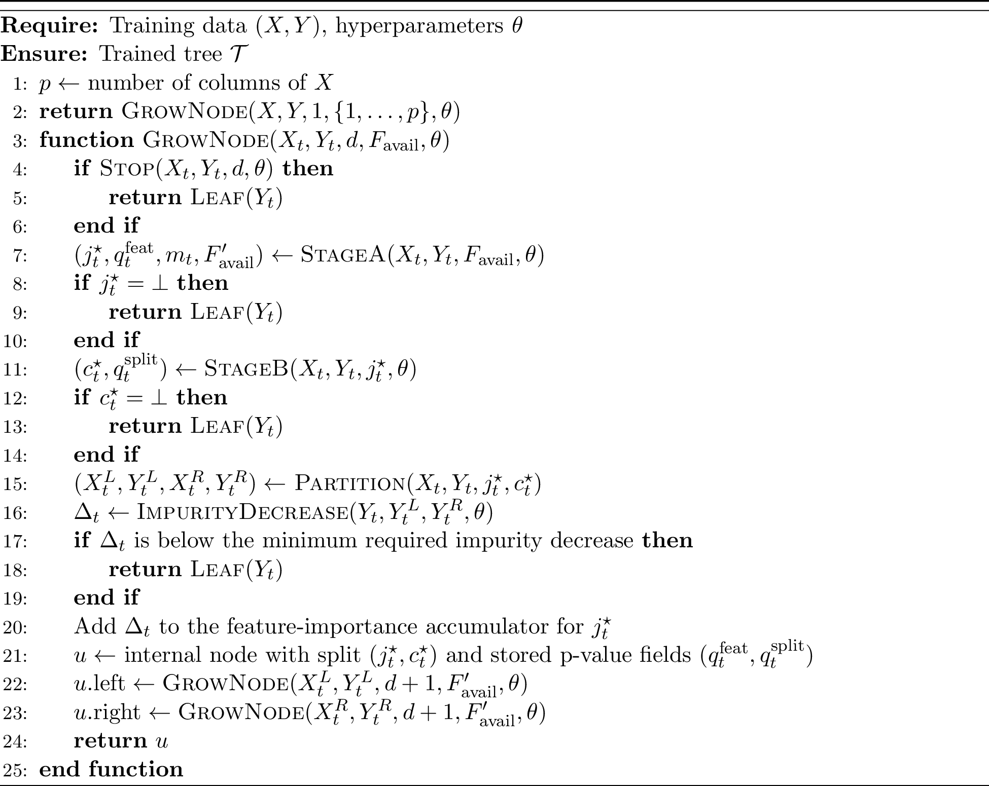
For the remaining finite threshold set \(C_{t,j_t^\star}\), Stage B selects the threshold used by the tree. The tested statistic at threshold \(c\) is the weighted child impurity \[\frac{|Y_t^L(c)|}{|Y_t|}\mathrm{Imp}(Y_t^L(c)) + \frac{|Y_t^R(c)|}{|Y_t|}\mathrm{Imp}(Y_t^R(c)),\] where \(\mathrm{Imp}\) is the chosen node impurity measure. This statistic is used in a left-tail test, and the exhaustive fixed-\(B\) rule chooses the threshold with the smallest Stage B \(p\)-value, with uniform tie breaking. During adaptive tree growing, threshold scanning may reorder thresholds and stop after the first rejecting threshold, so the returned Stage B score is a tree-construction score rather than a global minimum over all retained thresholds. Let \(\tau_t^{\mathrm{split}}=\alpha_{\mathrm{split}}/|C_{t,j_t^\star}|\) when Bonferroni is enabled for Stage B and \(\tau_t^{\mathrm{split}}=\alpha_{\mathrm{split}}\) otherwise. If no evaluated Stage B \(p\)-value is below \(\tau_t^{\mathrm{split}}\), the node becomes terminal. After a threshold passes the Stage B test, the final minimum required-improvement check uses the corresponding weighted impurity decrease. Stage B chooses the split used by the tree; the returned Stage B score is not a valid post-selection \(p\)-value. The training skeleton in 1 summarizes this flow and, for the benchmarked CIT and CIF configurations, stores two values at each split: the Stage A permutation \(p\)-value for the selected feature and the Stage B permutation \(p\)-value for the selected threshold.
2.2 Monte Carlo permutation \(p\)-values↩︎
Let \(T_{\mathrm{obs}}\) be the observed statistic and \(T_1,\dots,T_B\) the same statistic computed on \(B\) random label permutations. For a right tail test we use the Phipson–Smyth \(+1\) \(p\)-value [16], [17], where \(\mathbf{1}\{\cdot\}\) denotes the indicator function: \[p_{\mathrm{MC}}^{\ge} := \frac{1 + \sum_{b=1}^B \mathbf{1}\{T_b \ge T_{\mathrm{obs}}\}}{B+1}.\] For a left tail test we analogously define \[p_{\mathrm{MC}}^{\le} := \frac{1 + \sum_{b=1}^B \mathbf{1}\{T_b \le T_{\mathrm{obs}}\}}{B+1}.\] Stage A uses the right tail convention and Stage B the left tail convention; ties count as exceedances in both cases.
2.3 Forests and runtime hyperparameters↩︎
CIF combines bootstrap trees and averages their predictions. For feature selection, it sums each fitted tree’s normalized split importances and renormalizes the forest vector. Each CIF tree uses the same Stage A and Stage B node rules as CIT [12], [18]. The fixed-node theorem applies only to the Stage A reference test described above. Across the CIT/CIF benchmark configurations, we hold Bonferroni correction, adaptive stopping, feature muting, feature scanning, threshold scanning, histogram-256 thresholding, and CIF bootstrap sampling fixed. The varying settings are selector choice and honesty.
Runtime depends on the realized work at each node: features tested in Stage A, thresholds generated and retained in Stage B, permutations evaluated before stopping, and features carried into the node. Adaptive stopping changes the number of permutations evaluated for each test [19], [20]. Histogram thresholding reduces the Stage B threshold set by replacing exhaustive cutpoints with binned thresholds. Feature and threshold scanning change the order in which features or thresholds are tested under early stopping; feature muting can reduce the feature pool inherited by descendants. Appendix 12 gives algorithm and reproducibility details, Appendix 13 gives runtime and memory accounting, and 5.2 reports the measured timing effects.
2.4 Feature rankings↩︎
The experiments evaluate each method through the ranking it produces on the training fold. CIT and CIF rankings are fitted split-importance rankings, not rankings of Stage A \(p\)-values. For a fitted CIT, feature \(j\) receives the sum, over internal nodes that split on \(j\), of the impurity decrease at that node: parent impurity minus the weighted child impurity. If the total importance is positive, the vector is normalized to sum to one; if the tree contributes no positive impurity decrease, the vector remains zero. CIF sums these tree importance vectors over trees and then normalizes the forest vector in the same way. Stage A determines which features enter threshold optimization, while impurity decrease scores only the accepted splits by their local reduction in impurity. Larger importances are ranked earlier, and features never used by a split receive zero importance.
This split-importance ranking differs from standard random-forest impurity importance in how a feature enters threshold search. In CART-style trees, the feature and threshold are chosen together by an impurity search, so a feature with more possible thresholds has more chances to produce a large apparent impurity decrease [7]. In CIT and CIF, Stage A first selects a feature by a permutation test; Stage B then searches thresholds only for that feature. This reduces the advantage that high-cardinality features get from having more possible thresholds. We use these fitted split-importance scores as rankings and evaluate them through downstream top-\(k\) prediction and synthetic feature recovery.
3 Fixed-node Stage A control↩︎
This section analyzes the exhaustive fixed-\(B\) Stage A feature selection rule at a fixed node. The theorem proves superuniformity for a single \(+1\) Monte Carlo permutation \(p\)-value, and the corollary applies Bonferroni correction across the fixed-node Stage A tests. In the notation of 2.1, this is the reference case where every feature in \(F_t\) is tested with the same fixed nodewise budget \(B\). All probabilities below condition on \((X_t,U)\), where \(U\) collects label-independent auxiliary randomness other than the Monte Carlo permutation draws.
Theorem 1 (\(+1\) permutation \(p\)-values are superuniform). Assume A0.1 through A0.5 from 9.2. Under the nodewise complete permutation null at the fixed node \(t\), conditional on \((X_t,U)\), the observed statistic together with the \(B\) random-permutation statistics has the rank distribution of an exchangeable tuple of length \(B+1\). Define the right-tail \(+1\) Monte Carlo \(p\)-value \[p_{\mathrm{MC}}^{\ge} := \frac{1 + \sum_{b=1}^B \mathbf{1}\{T_b \ge T_{\mathrm{obs}}\}}{B+1}.\] Then for every \(\alpha \in [0,1]\), \[\mathbb{P}(p_{\mathrm{MC}}^{\ge} \le \alpha \mid X_t,U) \le \alpha.\]
This is the standard exchangeable-rank result for Monte Carlo permutation tests [16], [21], [22]. [app:permutation-exchangeability,app:proof-plusone] state the exchangeability condition and give the proof. The left-tail version follows by applying the same result to \(-T\).
Corollary 1 (Stage A complete null control at a fixed node). Assume A0.1 through A0.5 from 9.2. Under the nodewise complete null at \(t\), let \(F_t\) be nonempty and write \(m_t = |F_t| \ge 1\). Let Stage A reject when \[\min_{j \in F_t} p_{t,j} \le \alpha_{\mathrm{sel}}/m_t.\] The tree-growing rule uses a strict comparison, so its rejection event is a subset of the nonstrict event above. Then \[\mathbb{P}\!\left(\exists j \in F_t : p_{t,j} \le \alpha_{\mathrm{sel}}/m_t \,\middle|\, X_t,U\right) \le \alpha_{\mathrm{sel}}.\]
Combining 1 with the Bonferroni union bound over the \(m_t\) Stage A tests gives fixed-node Stage A control under the complete null. The result is local: it does not cover partial-null familywise error control, \(p\)-values for selected features, or error control for fitted trees and forests.
4 Experimental design↩︎
The experiments ask whether rankings produced by CIT and CIF place predictive features early enough for fixed downstream learners. For each training fold, a method produces a feature ranking, and fixed downstream learners evaluate the selected features on the held-out fold. We then summarize overall ranks, how often CIF performs well across datasets, high-dimensional behavior, recovery on synthetic data with known informative features, CIF ranking ablations, and feature sampling in forests.
4.1 Benchmark setup↩︎
The benchmark uses 5 random seeds, with 5-fold cross-validation within each seed. Classification fits logistic regression (LR), support vector machine (SVM), and k-nearest neighbors (KNN) as downstream models and reports balanced accuracy, defined as mean recall across classes. Regression fits ridge regression, support vector regression (SVR), and KNN and reports \(R^2\). The main tables use the standard values \(k \in \{5,10,25,50,100\}\). Downstream learner settings are fixed. Logistic regression uses balanced class weights and a 1,000-iteration limit; SVM uses an RBF kernel with unit regularization, \(\gamma=\texttt{scale}\), and balanced class weights; KNN uses 5 distance-weighted neighbors; ridge uses unit penalty strength; and SVR uses an RBF kernel with unit regularization, \(\epsilon=0.1\), and \(\gamma=\texttt{scale}\).
For each seed and fold, feature-standardization parameters are estimated on the training fold and then applied to the held-out fold. The ranking method uses only the standardized training fold and produces the ordered feature list described in 2.4. For each \(k\), we take the top-\(k\) features from that ranking, refit standardization on the selected training columns, apply the same transform to the selected held-out columns, fit the downstream model on the selected training data, and evaluate it on the held-out fold.
The downstream evaluation also records performance using the full feature set, \(k=p\), for every dataset. For datasets with more than 100 features, the separate high-\(p\) analysis adds fixed values \(k \in \{150,200,300,500,750,1{,}000\}\) and fractional values \(\lceil 0.25p\rceil,\lceil 0.5p\rceil,\lceil 0.75p\rceil\), keeping only values no larger than \(p\). The main tables average only the standard \(k\) values.
4.2 Benchmark comparisons↩︎
The benchmark averages scores in three steps. First, for each \((\text{dataset}, \text{downstream model}, k)\) combination, scores are averaged over folds and seeds. Second, each dataset score averages those fold-and-seed means over downstream models and over the standard \(k\) values available for the methods in that comparison. Third, the tables average dataset scores over datasets.
The real-data classification benchmark contains 23 datasets. Comparisons involving partykit ctree and cforest use the 22-dataset subset that excludes dexter; comparisons among methods with dexter results use all 23 datasets.
The complete-case classification analysis, used for bootstrap intervals and omnibus rank testing, contains 14 datasets with all 17 methods, all three downstream learners, and all five standard values of \(k\). Regression
contains 8 datasets; the analogous rank summary uses the 6 complete-case datasets with all methods, downstream learners, and standard \(k\) values available.
By-\(k\) results are reported separately for \(k=5,10,25,50,100\). The corresponding classification dataset counts are \(22, 21, 15, 15, 14\); the regression counts are \(8, 8, 7, 7, 6\). Pairwise CIF comparisons stratified by \(k\) use the dataset counts reported with the corresponding rows. The 14-dataset classification and 6-dataset regression summaries are complete-case analyses, retaining only datasets with every method, downstream learner, and standard \(k\) value.
4.3 Datasets↩︎
The real-data benchmark includes 23 classification datasets and 8 regression datasets. The separate high-\(p\) analysis restricts attention to the 15 classification datasets and 6 regression datasets with more than 100 features. The full inventories of the real and synthetic datasets are listed in 14, which also summarizes the synthetic designs and their parameter choices.
Feature recovery uses 8 synthetic classification datasets and 8 synthetic regression datasets with known informative features and controlled noise structure. A separate study of feature sampling uses \(n=250\) and varies \(p \in \{100, 500, 1{,}000\}\) and \(n_{\mathrm{informative}} \in \{1,2,5,10\}\). That study compares CIT, a CART decision tree (DT), a random threshold tree (RT), CIF, CIF-all, random forests (RF), and ExtraTrees (ET), using 1,000 trees for forest methods. CIF-all denotes the CIF variant that evaluates all nonconstant features at each split.
4.4 Compared methods↩︎
The benchmark includes three types of feature selectors: permutation-test filters, embedded tree or ensemble methods, and wrapper baselines. Permutation-test filters compute univariate dependence statistics and rank features by their permutation \(p\)-values: multiple correlation (MC) and randomized dependence coefficient (RDC) for classification, and Pearson correlation (PC), distance correlation (DC), and RDC for regression. The RDC filter keeps the empirical-CDF random feature map from [23] but replaces the canonical-correlation solve with the maximum absolute pairwise correlation across projected columns. Distance correlation follows [24].
Embedded methods rank features using tree or ensemble importance scores. These methods are CART decision trees (DT), randomized trees (RT), CIT, CIF, random forests (RF) [12], ExtraTrees [25], XGBoost [26], LightGBM [27], CatBoost [28], and the partykit reference implementations ctree and cforest [8], [29], [30]. Wrapper baselines score features through auxiliary random-forest fits: Boruta [31], permutation importance (PI) [7], [12], conditional permutation importance (CPI) [32], and random-forest recursive feature elimination (RF-RFE) [33], [34].
In this benchmark, CPI uses stratified conditional permutation with correlation-based strata. For each target feature, it trains a 100-tree random forest on a training split and scores a 20% validation split. It then identifies validation-set features with absolute correlation at least 0.5 with the target feature, forms five-bin percentile strata from those conditioning features, and permutes the target feature within strata. If no conditioning feature meets the correlation threshold, the target feature is permuted globally.
Ranking rules use each method’s natural score direction. Embedded tree and ensemble baselines rank features by decreasing fitted importance: DT, RT, RF, ExtraTrees, XGBoost, LightGBM, and CatBoost. Permutation-test filters rank by increasing \(p\)-value, with dependence score as the secondary key. The ctree reference ranks features by split-use counts. For cforest, we use partykit’s unconditional variable-importance scores with one permutation; CIF uses split-importance rankings from accepted conditional-inference splits. The cforest results therefore refer to this benchmarked partykit importance setting. Boruta and recursive feature elimination rank by their fitted rank variables, with smaller ranks first. PI and CPI rank by decreasing importance; the CPI row uses the stratified conditional-permutation procedure described above. Ties are broken by deterministic, method-specific order for reproducibility.
4.5 Configuration selection↩︎
Several methods, including CIT, CIF, XGBoost, LightGBM, ctree, and cforest, were evaluated under multiple configurations. Permutation-test filters used one configuration per statistic. For each task, the paper reports one configuration per method, selected by mean score over real datasets, downstream models, and the standard values \(k \in \{5,10,25,50,100\}\). Methods with only one configuration are treated as fixed. The selected configuration is then held fixed across datasets for that task. Because configuration selection and reporting use the same real-data benchmark, the reported scores, intervals, and rank summaries are descriptive. As a sensitivity check, we repeat configuration selection in leave-one-dataset-out (LODO) form for both tasks. In classification, each of the 14 complete-case datasets is evaluated using configurations chosen from the other 13 datasets. In regression, each of the 6 complete-case datasets is evaluated using configurations chosen from the other 5 datasets. The downstream models, \(k\) values, and averaging within each dataset are unchanged.
For the synthetic analysis, configurations are selected separately from the real-data benchmark. Each method is assigned the configuration with the highest average recovery of the true informative features over \(k = 5, 10, 25, 50,\) and \(100\). The benchmarked CIT and CIF configurations use adaptive sequential stopping, Bonferroni correction, feature muting, feature scanning, threshold scanning, and 256-bin histogram thresholding. The benchmarked CIT and CIF variants differ in selector and honesty; CIF is run as a bootstrap forest. Each CIF runtime ablation changes one setting.
To isolate which parts of the CIF ranking matter, we run a ranking ablation on the real-data benchmark datasets. The ablation holds the selected CIF configuration fixed and changes one component at a time: replacing fitted split importance with split counts, disabling feature muting, disabling bootstrap sampling, or reducing the forest to one tree. Each variant is evaluated with the same downstream learners, folds, seeds, and standard top-\(k\) values as the main benchmark.
5 Results↩︎
5.1 Real-data benchmark↩︎
1 reports the main real-data comparison. Classification uses the 22 datasets with ctree and cforest results; the full classification collection has 23 datasets, with dexter reserved for analyses
that compare methods available on that dataset. Regression uses all 8 datasets. Within each dataset, scores are first averaged over downstream learners and the standard \(k\) values shared by the compared methods, then
converted to ranks. Lower mean rank is better.
| Classification | Regression | ||||||||||||||||||||||||||||||||||||||
|---|---|---|---|---|---|---|---|---|---|---|---|---|---|---|---|---|---|---|---|---|---|---|---|---|---|---|---|---|---|---|---|---|---|---|---|---|---|---|---|
| 1-2(l)3-4 Method | Mean rank | Method | Mean rank | ||||||||||||||||||||||||||||||||||||
| LightGBM | 5.17 | ExtraTrees | 6.56 | ||||||||||||||||||||||||||||||||||||
| XGBoost | 5.58 | CatBoost | 6.97 | ||||||||||||||||||||||||||||||||||||
| CatBoost | 5.85 | CIF | 7.07 | ||||||||||||||||||||||||||||||||||||
| CIF | 6.08 | RF | 8.09 | ||||||||||||||||||||||||||||||||||||
| RF | 6.27 | RT | 8.37 | ||||||||||||||||||||||||||||||||||||
| RF-RFE | 6.98 | DT | 8.68 | ||||||||||||||||||||||||||||||||||||
| ExtraTrees | 7.45 | LightGBM | 8.76 | ||||||||||||||||||||||||||||||||||||
| DT | 7.67 | RDC filter | 8.83 | ||||||||||||||||||||||||||||||||||||
| RT | 10.05 | CIT | 9.19 | ||||||||||||||||||||||||||||||||||||
| CIT | 10.34 | PC filter | 9.35 | ||||||||||||||||||||||||||||||||||||
| Boruta | 10.51 | DC filter | 9.77 | ||||||||||||||||||||||||||||||||||||
| MC filter | 10.65 | XGBoost | 9.96 | ||||||||||||||||||||||||||||||||||||
| PI | 10.76 | Boruta | 10.00 | ||||||||||||||||||||||||||||||||||||
| cforest | 11.36 | PI | 10.19 | ||||||||||||||||||||||||||||||||||||
| RDC filter | 12.29 | RF-RFE | 10.41 | ||||||||||||||||||||||||||||||||||||
| ctree | 12.86 | cforest | 12.20 | ||||||||||||||||||||||||||||||||||||
| CPI | 13.13 | ctree | 12.99 | ||||||||||||||||||||||||||||||||||||
| CPI | 13.61 | ||||||||||||||||||||||||||||||||||||||
With selected configurations fixed, CIF ranks 4th of 17 classification methods and 3rd of 18 regression methods. 2 compares CIF directly with ctree, cforest, and CIT. 15 gives the learner-by-\(k\) tables (16 17), pairwise CIF-comparison heatmaps (7 8), and seed-sensitivity tables (18 19); each analysis reports its dataset count.
| Task | Compared with | Datasets | Mean diff. | W–L | |||||||||||||||||||||||||||||||||||||
|---|---|---|---|---|---|---|---|---|---|---|---|---|---|---|---|---|---|---|---|---|---|---|---|---|---|---|---|---|---|---|---|---|---|---|---|---|---|---|---|---|---|
| Classification | ctree | 22 | +0.088 | ||||||||||||||||||||||||||||||||||||||
| Classification | cforest | 22 | +0.072 | ||||||||||||||||||||||||||||||||||||||
| Classification | CIT | 23 | +0.032 | ||||||||||||||||||||||||||||||||||||||
| Regression | ctree | 8 | +0.226 | ||||||||||||||||||||||||||||||||||||||
| Regression | cforest | 8 | +0.721 | ||||||||||||||||||||||||||||||||||||||
| Regression | CIT | 8 | +0.360 |
5pt
2 shows CIF ahead on average in all six direct pairings. On the complete-case datasets, CIF is also ahead of ctree, cforest, and CIT in both tasks. The 95% bootstrap CIs for mean CIF-minus-comparator differences are as follows. Classification (14 datasets): ctree [+0.068, +0.154], cforest [+0.067, +0.160], CIT [+0.023, +0.060]. Regression (6 datasets): ctree [+0.113, +0.529], cforest [+0.040, +2.570], CIT [-0.007, +1.224]. The regression interval for CIF versus CIT crosses zero; the other complete-case intervals are positive. The regression intervals are wider because fewer datasets are available and some comparator mean \(R^2\) values are negative.
5.1.0.1 CIF ablations.
3 compares the selected CIF configuration with four targeted changes: split-count ranking, disabling bootstrap sampling, disabling feature muting, and using one tree.
| Task | CIF change | Mean diff. | 95% CI | W–L | |||||||||||||||||||
|---|---|---|---|---|---|---|---|---|---|---|---|---|---|---|---|---|---|---|---|---|---|---|---|
| Classification | Split-count ranking | -0.003 | [-0.007, +0.001] | 10–13 | |||||||||||||||||||
| Classification | Disable bootstrap | +0.001 | [-0.003, +0.004] | 10–12 | |||||||||||||||||||
| Classification | Disable feature muting | +0.000 | [-0.001, +0.002] | 13–8 | |||||||||||||||||||
| Classification | Use one tree | -0.061 | [-0.091, -0.035] | 1–22 | |||||||||||||||||||
| Regression | Split-count ranking | -0.022 | [-0.060, +0.000] | 3–5 | |||||||||||||||||||
| Regression | Disable bootstrap | -0.208 | [-0.604, -0.004] | 3–5 | |||||||||||||||||||
| Regression | Disable feature muting | +0.000 | [-0.011, +0.009] | 5–3 | |||||||||||||||||||
| Regression | Use one tree | -0.552 | [-1.328, -0.073] | 0–8 |
4pt
Reducing CIF to one tree has the largest effect: \(-0.061\) balanced accuracy in classification and \(-0.552\) \(R^2\) in regression. Replacing fitted split importance with split counts changes the mean score by \(-0.003\) in classification and \(-0.022\) in regression, with intervals that include zero. Disabling feature muting changes both tasks by \(+0.000\), while disabling bootstrap sampling changes classification by \(+0.001\) and regression by \(-0.208\).
The complete-case Friedman tests use dataset-level method means. Classification: \(\chi^2(16)=141.32\), \(p<0.001\), Kendall’s \(W=0.63\). Regression: \(\chi^2(17)=33.79\), \(p=0.0089\), Kendall’s \(W=0.33\). The regression panel has 6 datasets, so the \(p\)-value should be read with the effect sizes, intervals, and LODO results. These intervals and rank tests summarize the benchmark-selected configurations. The LODO analysis below checks whether those configurations are stable under one-dataset holdout.
In the 14-dataset classification panel, LODO ranks CIF fifth of 17 on average (mean rank 5.64), and CIF reselects the main-benchmark configuration in all 14 holdouts. In the 6-dataset regression panel, LODO ties CIF with CatBoost for second on average (mean rank 5.50), behind ExtraTrees; CIF reselects the global regression configuration in 5 of 6 holdouts. [tab:cif-ci-comparisons,tab:lodo-config-sensitivity] give the confidence intervals and LODO details.
4 reports how often CIF appears in the top half or top 3 and how often it beats tree baselines.
| Summary | Classification | Regression |
|---|---|---|
| Main rank | ||
| Top half | ||
| Top 3 | ||
| Win vs ctree | ||
| Win vs cforest | ||
| Win vs CIT | ||
| Win vs DT | ||
| Win vs RT |
6pt
In classification, CIF is in the top half on 21 of the 22 datasets with ctree and cforest results, and in the top 3 on 5 of 22. In regression, CIF is in the top half on 6 of 8 datasets and in the top 3 on 2 of 8. Against the greedy single-tree baselines, CIF beats DT on 14/23 classification datasets and 6/8 regression datasets, and beats RT on 21/23 classification datasets. The RT regression comparison is close: CIF is ahead on 5/8 datasets, with a mean difference near zero.
[fig:k-trajectory,fig:regression-k-trajectory] report mean rank separately by \(k\). In classification, CIF’s mean rank is 6.2 at \(k=5\), 7.4 at \(k=10\), 5.5 at \(k=50\), and 5.0 at \(k=100\). In regression, CIF’s mean rank is 8.9 at \(k=5\), 5.6 at \(k=50\), and 7.3 at \(k=100\). These by-\(k\) results add context to 1: CIF is strongest at larger displayed \(k\) values in classification and at \(k=50\) in regression. The aggregate ctree and cforest comparisons use 22 classification datasets. For \(k=5,10,25,50,100\), the classification columns use 22, 21, 15, 15, and 14 datasets, respectively; the regression columns use 8, 8, 7, 7, and 6 datasets, respectively. Complete-case analyses use 14 classification datasets and 6 regression datasets.


5.2 Runtime ablations↩︎
The runtime ablations identify which benchmark settings have the largest effect on fitting time and report how much the ranking scores move when those settings change. Each row changes one setting and reports elapsed wall-clock fit time relative to the selected configuration for the same estimator. Ratios above 1 are slower than that reference, and ratios below 1 are faster. CIT and CIF are shown separately because the CIT run records fit time and synthetic top-10 feature recovery, while the CIF runs also record downstream score changes. The main benchmark remains the primary performance comparison. 13 links each ablation to the affected work terms.
| CIT change | Runtime ratio | |
| F1 change | ||
| Disable adaptive stopping | 0.18–1.14\(\times\) | \(\le 0.026\) |
| Exact threshold search | 0.98–2.51\(\times\) | \(\le 0.008\) |
| Disable feature scanning | 0.69–1.46\(\times\) | \(\le 0.017\) |
6pt
5.2.0.1 CIT runtime ablations.
5 shows that CIT timing effects vary by data regime. Disabling adaptive stopping reduces runtime in the synthetic runs and has less consistent timing on real datasets. For a single fitted tree, changing this option can also change the realized sequence of features, thresholds, and nodes evaluated. These rows focus on timing and synthetic feature-recovery changes.
| CIF change | Runtime ratio | ||
| score change | |||
| recovery change | |||
| Disable adaptive stopping | 4.0–8.4\(\times\) | \(\le 0.006\) | \(\le 0.006\) |
| Exact threshold search | 1.9–10.8\(\times\) | \(\le 0.011\) | \(\le 0.017\) |
| Disable feature scanning | 0.89–1.83\(\times\) | \(\le 0.006\) | \(\le 0.010\) |
6pt
5.2.0.2 CIF runtime ablations.
6 shows consistent slowdowns for two CIF changes. Disabling adaptive stopping makes fits 4.0–8.4\(\times\) slower by median dataset-level ratios. In the separate threshold-search ablation, exact threshold search is 1.9–10.8\(\times\) slower than histogram-256 by ratios of group mean elapsed times. Downstream score changes and synthetic feature-recovery changes are at most 0.011 and 0.017. The feature-scanning effect is smaller and less consistent once adaptive stopping is enabled. Removing Bonferroni correction is faster for both CIT and CIF, but it changes the statistical rule and yields trees with more selected features; the selected setting keeps Bonferroni correction.
6 High-dimensional and synthetic analyses↩︎
6.0.0.1 High-dimensional real datasets.
These analyses study where CIF’s scores peak as \(k\) grows, how feature recovery on synthetic datasets changes across values of \(k\), and how feature sampling inside the forest affects how often splits use informative features. Across the 15 classification datasets with more than 100 features, CIF first reaches its best score at an intermediate value of \(k\) (\(100 < k < p\)) in 30 of 45 dataset-learner combinations. It first reaches its best score at the full feature set (\(k=p\)) in only 5 of 45 combinations. 4 shows this pattern by downstream learner; regression is summarized next. Classification scores most often peak at intermediate \(k\): 11 of 15 LR datasets, 9 of 15 SVM datasets, and 10 of 15 KNN datasets. The full feature set is mainly an LR exception. Moving from \(k{=}100\) to \(k{=}p\) gives a mean \(k{=}p\) minus \(k{=}100\) score change of \(+0.022\) for LR, and \(k=p\) matches the best observed LR score in 6 of 15 datasets. For SVM and KNN, the corresponding mean changes are \(-0.058\) and \(-0.075\), and \(k=p\) is best in only 1 of 15 datasets for each learner.
In the 6 high-\(p\) regression datasets, full-feature evaluation is rarely best. Across the 18 dataset-learner combinations, 11 peak at or below \(k{=}100\), only 2 peak at \(k=p\), and the mean \(k{=}p\) minus \(k{=}100\) score change is \(-0.308\). The main full-feature exception remains the classification LR result in 4.

6.0.0.2 Synthetic feature recovery.
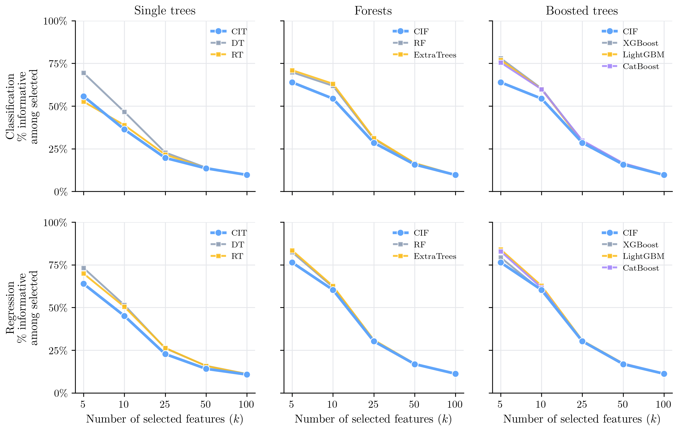
Across synthetic classification datasets, 34% of the features in CIF’s top-\(k\) list are truly informative on average over the evaluated \(k\) values, ranked 8th of 17, and its top-1 hit rate is 64%, ranked 12th of 17. Across synthetic regression datasets, the corresponding values are 39%, ranked 10th of 18, and 81%, ranked 15th of 18. In both tasks, CIF recovers true features within the top-\(k\) list more reliably than it places one first. 7 summarizes this contrast, and 5 shows recovery as \(k\) grows. The percentage of selected features that are informative falls as \(k\) grows. On redundant-feature synthetic designs, most selected features correspond to true signals or redundant proxies: 83% for classification and 84% for regression.
| Classification | Regression | |||
|---|---|---|---|---|
| 2-3(l)4-5 Metric | Value | Rank | Value | Rank |
| Selected features that are informative | 34% | 39% | ||
| Top-1 hit rate | 64% | 81% | ||
| Selected features that are true or redundant | 83% | 84% | ||
6pt
6.0.0.3 Feature sampling in forests.
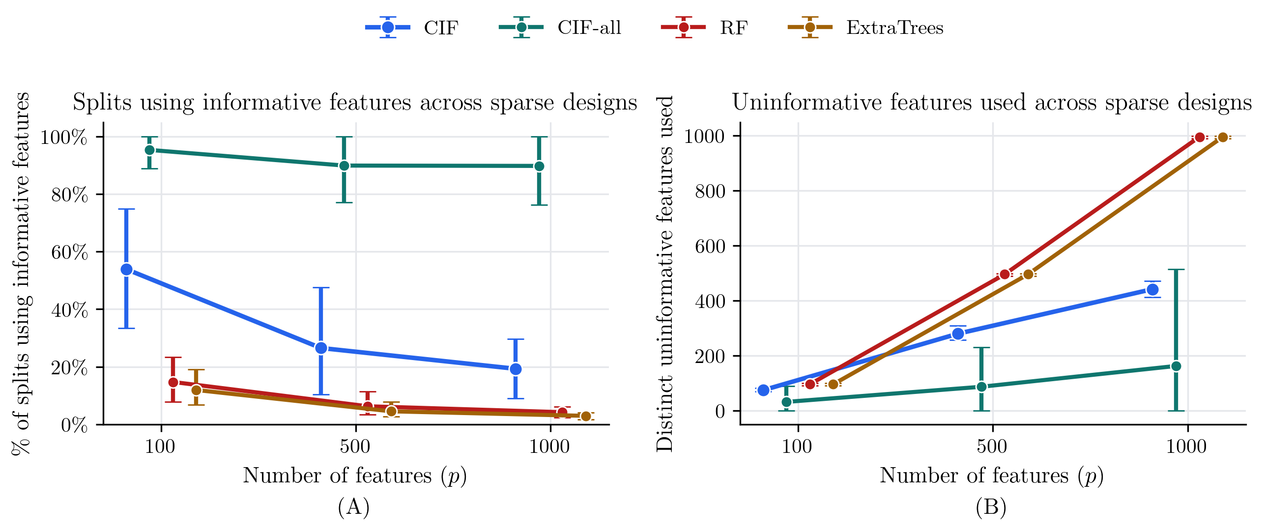
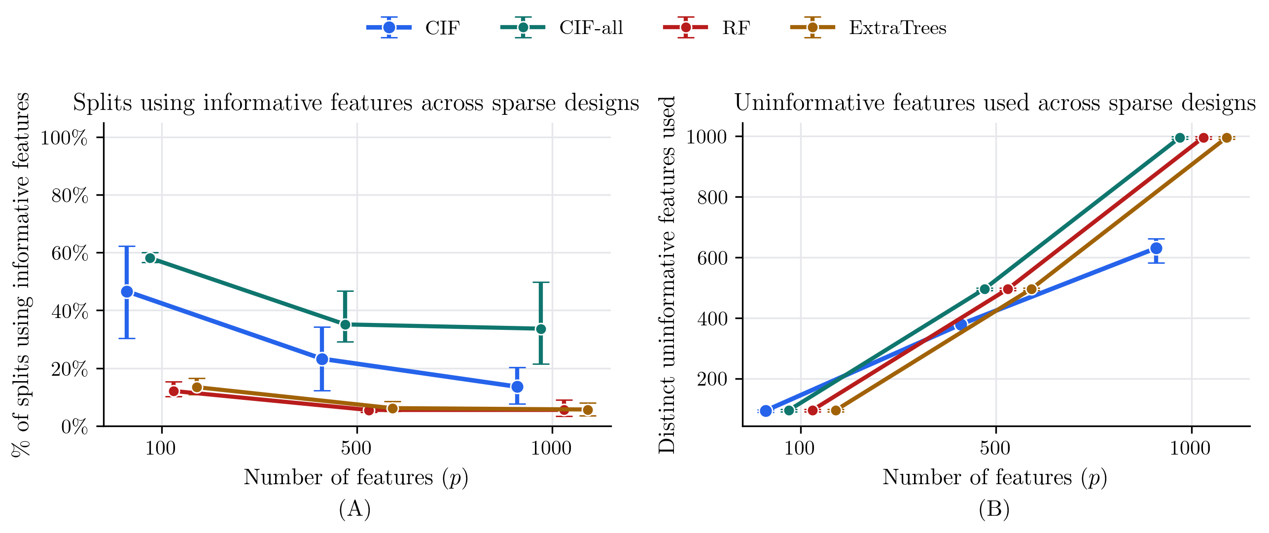
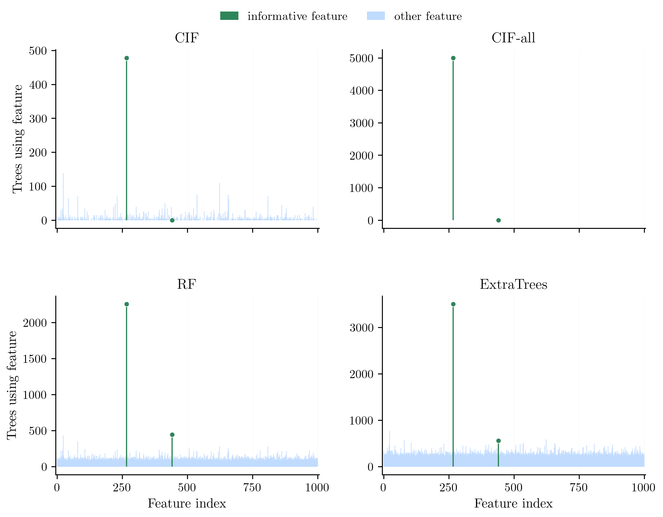
A sparse simulation asks whether forest feature sampling makes splits less likely to use informative features in classification and regression settings. 6 shows one sparse classification design comparing CIF with CIF-all. CIF samples a subset of features at each split; CIF-all considers every nonconstant feature in Stage A. 16 gives the classification and regression results over \(p \in \{100,500,1{,}000\}\).
In the single-tree simulations, CIT uses informative features in 100.0% of classification splits and 93.5% of regression splits. In this fixed design, informative features are usually selected when every nonconstant feature is considered. In forests, sampling a subset of features reduces how often informative features are used for splits. Across the classification forest simulations with 1,000 trees, CIF uses informative features in 33.2% of splits, compared with 91.7% for CIF-all, 8.4% for RF, and 6.5% for ET. CIF also uses more distinct noise features than CIF-all, 265 versus 93 on average. For the \(p{=}1{,}000\) classification setting with two informative features, CIF uses informative features in 9.0% of splits, while CIF-all uses them in 100.0%. In regression, CIF-all uses informative features more often than CIF, 42.3% versus 27.8%, but uses more distinct noise features, 528.8 versus 367.7. CIF-all isolates feature subsampling because feature muting and the other tree settings are held fixed. In these sparse high-\(p\) simulations, splits use informative features most often when every nonconstant feature can enter Stage A. When the sampled feature subset rarely includes an informative feature at a node, Stage A selects from that subset.
7 Discussion↩︎
In these experiments, CIF is best supported as a top-\(k\) feature-selection method for a downstream model. The benchmark asks whether a ranking places predictive features early enough for fixed downstream learners. Classification gives the clearest support; the smaller regression panel is positive but less precise. The fixed-node Stage A theorem provides the local guarantee; fitted tree and forest rankings are assessed empirically.
7.0.0.1 Guidance.
A CIF ranking should be judged through the downstream model that will use the selected features. In practice, choose \(k\) on held-out data over a small set of values that includes the intended feature budget and, when feasible, the full feature set as a sanity check. When prediction accuracy is the main target, tree-ensemble baselines such as random forests, ExtraTrees, and boosted trees should remain in the comparison set. When the target is variable screening or a ranked feature list for later modeling, CIF should also be compared with ctree, cforest, and forest-based screening methods such as Boruta, permutation or conditional permutation importance, and RF-RFE [11].
The ablations show that adaptive stopping and histogram-256 thresholding account for the largest measured CIF runtime changes, with small downstream score changes in these experiments. Bonferroni correction is part of the Stage A testing rule and is not treated as a runtime shortcut. For ranking quality, forest size matters more than the split-count and feature-muting variants tested here, so the selected CIF configuration is the relevant ranking reference when ranking quality is the priority.
In sparse high-\(p\) settings, feature use should be monitored directly. The simulations show that CIF feature sampling can leave informative features out of many forest split decisions, especially in sparse classification designs. Useful diagnostics include top-\(k\) stability across seeds, the share of splits using the final top-\(k\) features or any prespecified positive control features, the number of distinct low-ranked or known null features used in splits, and sensitivity to larger sampled feature sets or to a small CIF-all run with fewer seeds or trees.
7.0.0.2 Limitations.
The fixed-node result is a reference guarantee for exhaustive fixed-\(B\) Stage A testing at one node, with the tested features and permutation budget fixed independently of the node responses. The benchmarked trees and forests add adaptive stopping, feature and threshold ordering, feature muting, bounded threshold sets, bootstrap samples, and forest aggregation, so their behavior is assessed through the ranking benchmark.
The benchmark coverage is uneven across analyses. Some comparisons use broader panels where both methods are available, while complete-case rank and interval summaries use smaller panels that include every method. These summaries are therefore descriptive rather than confirmatory.
The sampled-forest analysis isolates a sparse high-\(p\) setting in which forest feature sampling can limit how often splits use informative features: larger sampled feature sets increase informative-feature use, but they also change runtime and the mix of noise features used by splits. Track how often splits use informative features alongside downstream performance and runtime before changing the number of features sampled at each split.
8 Conclusion↩︎
This paper evaluates conditional-inference tree and forest rankings for top-\(k\) downstream prediction and proves a fixed-node guarantee for Stage A permutation testing. The experiments support CIF as a top-\(k\) feature-ranking method, especially in classification: its rankings compare favorably with ctree, cforest, and CIT, and they remain competitive among stronger tree-ensemble baselines.
The ablations separate runtime and ranking effects. Adaptive stopping and bounded threshold search avoid large runtime increases, while the one-tree ablation has the largest ranking-quality loss. The high-\(p\) and synthetic analyses add two diagnostic cautions: sparse forests should be checked for whether informative features are used in enough splits to enter the top-\(k\) ranking, and CIF should not be treated as a first-feature discovery method when the goal is to identify a single driver. Overall, these results support CIF as a feature-ranking method for downstream prediction, backed by a local Stage A result and benchmark evidence.
9 Setup and assumptions↩︎
9.1 Fixed-node setup↩︎
Let \((X_i, Y_i)_{i=1}^n\) be the training data. Fix a node \(t\) with sample index set \(I_t\) and size \(n_t:=|I_t|\). Write \(X_t := (X_i)_{i\in I_t}\) and \(Y_t := (Y_i)_{i\in I_t}\) for the data restricted to that node. Stage A tests features \(F_t\) with \(m_t:=|F_t|\).
The fixed-node theorem analyzes the exhaustive fixed-\(B\) Stage A reference test. Conditional on the node covariates and label-independent auxiliary randomness \(U\), \(F_t\) and \(B\) are fixed, and every feature in \(F_t\) is tested with exactly \(B\) permutations.
Notation↩︎
8 lists the notation used in the proof.
| Symbol | Meaning |
|---|---|
| \(t\) | Node index, held fixed in the theorem. |
| \(I_t,\;n_t\) | Node sample index set and size \(n_t:=|I_t|\). |
| \(X_t,\;Y_t\) | Covariates and labels restricted to node \(t\). |
| \(U\) | Label-independent auxiliary randomness conditioned on in the proof; it excludes node responses, Monte Carlo permutation draws, permutation statistics, and \(p\)-values. |
| \(F_t,\;m_t\) | Stage A features and size \(m_t:=|F_t|\). |
| \(X_{t,j}\) | Values of feature \(j\) on the node samples. |
| \(B\) | Number of random label permutations per tested feature in the fixed-\(B\) reference test. |
| \(T^{\mathrm{sel}}_j\) | Stage A selector statistic for feature \(j\): \(T^{\mathrm{sel}}_j(X_{t,j},Y_t;U)\). |
| \(T(\cdot,\cdot;U)\) | Generic scalar test statistic used in the exchangeability proof. |
| \(\Pi_b\) | Random label permutation used for Monte Carlo replicate \(b\). |
| \(T_{\mathrm{obs}},T_1,\dots,T_B\) | Observed and permuted statistics for one fixed feature test. |
| \(R\) | Right-tail rank numerator \(1+\sum_{b=1}^B \ind\{T_b \ge T_{\mathrm{obs}}\}\). |
| \(p_{\mathrm{MC}}^{\ge}\) | Right-tail \(+1\) Monte Carlo permutation \(p\)-value for one fixed feature test. |
| \(p_{t,j}\) | Fixed-\(B\) \(+1\) Monte Carlo permutation \(p\)-value for feature \(j\). |
| \(\alpha_{\mathrm{sel}}\) | Stage A nominal level; the corollary tests at \(\alpha_{\mathrm{sel}}/m_t\). |
5pt
The guarantee applies only to fixed-node Stage A. It does not cover Stage B threshold search, adaptive stopping, response-dependent feature muting, response-selected internal nodes, bootstrap forests, honesty, or \(p\)-values after feature selection or other post-selection steps; see [sec:method] [app:methods] [app:complexity-details].
9.2 Assumptions and theorem scope↩︎
9.2.0.1 A0.1 (Fixed node).
Assumptions A0.1–A0.5 define the fixed-node reference setting used by Theorem 1 and Corollary 1. The node \(t\) and its sample index set \(I_t\) are held fixed for the result. They are not chosen using node responses or earlier response-dependent splits.
9.2.0.2 A0.2 (Complete nodewise permutation null).
Under the complete null at node \(t\), \(Y_t\) is exchangeable conditional on \((X_t,U)\): its conditional law is unchanged by permuting the node responses. This complete nodewise permutation null does not cover a null feature when any tested or untested node covariate remains associated with \(Y_t\).
9.2.0.3 A0.3 (Features fixed before seeing node responses).
The features in \(F_t\) and the effective nodewise budget \(B\) are measurable functions of \((X_t,U)\) only. They do not depend on \(Y_t\), other training responses used to reach the node, Monte Carlo permutation draws or statistics, \(p\)-values, or sequential stopping decisions.
9.2.0.4 A0.4 (Fixed-\(B\) computation).
Each \(p_{t,j}\) is computed with exactly \(B\) random permutations, with no optional stopping. The Monte Carlo permutation draws used to compute the \(p\)-values are additional randomness, independent of \((X_t,Y_t,U)\), and are not included in \(U\).
9.2.0.5 A0.5 (Conservative ties).
For right-tail tests, the Stage A \(+1\) Monte Carlo \(p\)-value counts ties conservatively using \(\mathbf{1}\{T_b \ge T_{\mathrm{obs}}\}\). If several features tie after testing, any random tie break is label-independent and does not affect the Stage A reject/no-reject event.
9.3 Results using these assumptions↩︎
Both fixed-node results in 3 use Assumptions A0.1–A0.5. Theorem 1 proves \(+1\) Monte Carlo permutation \(p\)-value superuniformity. Corollary 1 gives Stage A complete-null control.
10 Monte Carlo permutation exchangeability↩︎
The proof separates two facts. First, statistics computed from i.i.d. random permutations are exchangeable. Second, under A0.2–A0.4, the usual “observed statistic + \(B\) random permutations” computation has the same null rank distribution as a construction with a randomized baseline. The superuniformity proof then uses the conservative tie convention in A0.5; see also [22] for a broader treatment of exact random permutation testing.
First consider a fully randomized tuple. Fix a node \(t\), feature \(j\), and a real-valued statistic \(T(\cdot, \cdot; U)\) with a right tail convention (larger is more extreme), where \(U\) denotes label-independent auxiliary randomness. Let \(\Pi_0, \Pi_1, \dots, \Pi_B\) be i.i.d.uniform random permutations of \(\{1,\dots,n_t\}\), independent of the data (and of \(U\)), and define \[T_b := T(X_{t,j}, \Pi_b(Y_t); U) \qquad (b=0,1,\dots,B).\]
Lemma 1 (Exchangeability of Monte Carlo permutation statistics). Conditional on \((X_t, Y_t, U)\), the vector \((T_0, T_1, \dots, T_B)\) is exchangeable. Averaging over \(Y_t\) preserves exchangeability, so the vector is also exchangeable conditional on \((X_t,U)\) and unconditionally.
Proof. Conditional on \((X_t, Y_t, U)\), each \(T_b\) is a measurable function of \(\Pi_b\), and \((\Pi_0,\dots,\Pi_B)\) are i.i.d. Thus any permutation of the indices \(b \in \{0,\dots,B\}\) leaves the joint law unchanged. ◻
Lemma 2 (The observed statistic has the same null rank distribution). Assume A0.2–A0.4 (9.2). Let \(\Pi_1,\dots,\Pi_B\) be i.i.d. uniform random permutations of \(\{1,\dots,n_t\}\), independent of \((X_t,Y_t,U)\). Define the observed statistic and permuted statistics by \[T_{\mathrm{obs}} := T(X_{t,j}, Y_t; U), \qquad T_b := T(X_{t,j}, \Pi_b(Y_t); U) \quad (b=1,\dots,B),\] and the standard +1 Monte Carlo \(p\)-value (right tail) by \[p_{\mathrm{id}} := \frac{1 + \sum_{b=1}^B \mathbf{1}\{T_b \ge T_{\mathrm{obs}}\}}{B+1}.\] Let \(\Pi_0\) be an additional independent uniform random permutation and set \(T_0 := T(X_{t,j}, \Pi_0(Y_t); U)\) (keeping \(T_1,\dots,T_B\) as above), and define \[p_{\mathrm{rnd}} := \frac{1 + \sum_{b=1}^B \mathbf{1}\{T_b \ge T_0\}}{B+1}.\] Both quantities use the same conservative right-tail tie convention: ties with the baseline statistic are counted as exceedances. Under the null, conditional on \((X_t,U)\), \(p_{\mathrm{id}}\) and \(p_{\mathrm{rnd}}\) have the same distribution with this convention. It is enough to prove the rank bound for the exchangeable construction \(p_{\mathrm{rnd}}\) and apply the same conclusion to the standard “observed statistic + \(B\) random permutations” computation.
Proof. Fix \((X_t,U)\) and work under the null. By A0.2, permuting the node labels does not change the conditional distribution of \(Y_t\). Use the permutation-action convention under which \((\Pi_b \circ \Pi_0^{-1})(\Pi_0(Y_t)) = \Pi_b(Y_t)\). Let \(\Pi_0\) be an independent uniform permutation and set \(Y_t' := \Pi_0(Y_t)\). Then \(Y_t' \stackrel{d}{=} Y_t\) conditional on \((X_t,U)\).
For \(b=1,\dots,B\), define \(\Pi_b' := \Pi_b \circ \Pi_0^{-1}\), so \(\Pi_b'(Y_t') = \Pi_b(Y_t)\). Conditional on \((Y_t,\Pi_0)\), right composition by \(\Pi_0^{-1}\) maps the independent uniform permutations \(\Pi_b\) to independent uniform permutations \(\Pi_b'\). This conditional law does not depend on the conditioning values. Because \(Y_t'\) is a function of \((Y_t,\Pi_0)\), the transformed permutations are independent of \((Y_t',\Pi_0)\). Therefore, \[\begin{align} \big(T_{\mathrm{obs}}, T_1,\dots,T_B\big) &= \big(T(X_{t,j},Y_t;U), T(X_{t,j},\Pi_1(Y_t);U),\dots,T(X_{t,j},\Pi_B(Y_t);U)\big) \\ &\stackrel{d}{=} \big(T(X_{t,j},Y_t';U), T(X_{t,j},\Pi_1'(Y_t');U),\dots,T(X_{t,j},\Pi_B'(Y_t');U)\big) \\ &= \big(T_0, T_1,\dots,T_B\big), \end{align}\] where \(\stackrel{d}{=}\) is conditional on \((X_t,U)\). Applying the same \(\ge\) comparison map to these equal-in-distribution vectors gives the same conditional distribution for \(p_{\mathrm{id}}\) and \(p_{\mathrm{rnd}}\). ◻
11 Proof of Theorem 1↩︎
10 reduces the usual computation with one observed statistic and \(B\) random permutations to the exchangeable rank construction. We prove Theorem 1 under A0.1–A0.5 (9.2).
Fix \((X_t,U)\), fix one feature \(j \in F_t\), and work under the nodewise complete permutation null at the fixed node \(t\). Under A0.2–A0.4, the standard fixed-\(B\) computation has the same conditional \(p\)-value distribution as the randomized exchangeable construction; see 2 in 10 and [22]. It is enough to prove the rank bound for an exchangeable tuple, which we denote by \((T_{\mathrm{obs}},T_1,\dots,T_B)\).
Define the conservative right-tail rank numerator \[R := 1 + \sum_{b=1}^B \mathbf{1}\{T_b \ge T_{\mathrm{obs}}\}, \qquad p_{\mathrm{MC}}^{\ge} = \frac{R}{B+1}.\] The left-tail version replaces the exceedance check by \(\mathbf{1}\{T_b \le T_{\mathrm{obs}}\}\); equivalently, apply the right-tail argument below to \(-T\). Stage B uses this left-tail convention for split scores after Stage A selects a feature, but the fixed-node Type I error guarantee here concerns Stage A.
11.0.0.1 No ties.
If the statistics almost surely have no ties, then the \(\ge\) indicator is the same as \(>\), and \(R\) is the descending rank of \(T_{\mathrm{obs}}\) among \((T_{\mathrm{obs}},T_1,\dots,T_B)\), with rank 1 assigned to the largest statistic. Exchangeability implies \[\mathbb{P}(R = r \mid X_t,U) = \frac{1}{B+1}, \qquad r=1,\dots,B+1,\] so for any \(\alpha \in [0,1]\), \[\mathbb{P}(p_{\mathrm{MC}}^{\ge} \le \alpha \mid X_t,U) = \mathbb{P}\!\big(R \le (B+1)\alpha \mid X_t,U\big) = \frac{\lfloor (B+1)\alpha \rfloor}{B+1} \le \alpha.\]
11.0.0.2 Ties.
If ties can occur, A0.5 uses conservative tie handling: the right-tail \(+1\) \(p\)-value uses \(\mathbf{1}\{T_b \ge T_{\mathrm{obs}}\}\), so ties with the observed statistic are counted in the numerator. To compare this rule with a no-ties rank, let \(V_{\mathrm{obs}},V_1,\dots,V_B \stackrel{\mathrm{i.i.d.}}{\sim} \mathrm{Unif}(0,1)\) be independent of all other randomness and define augmented statistics \(\tilde{T}_{\mathrm{obs}} := (T_{\mathrm{obs}}, V_{\mathrm{obs}})\) and \(\tilde{T}_b := (T_b, V_b)\) for \(b=1,\dots,B\). Order the augmented pairs lexicographically for the right tail: \(\tilde{T}_b\) exceeds \(\tilde{T}_{\mathrm{obs}}\) exactly when \(T_b > T_{\mathrm{obs}}\), or when \(T_b = T_{\mathrm{obs}}\) and \(V_b > V_{\mathrm{obs}}\). Then \((\tilde{T}_{\mathrm{obs}},\tilde{T}_1,\dots,\tilde{T}_B)\) is exchangeable and almost surely has no ties, so the no-ties argument gives a superuniform \(p\)-value \[\tilde{p}_{\mathrm{MC}}^{\ge} := \frac{ 1 + \sum_{b=1}^B \mathbf{1}\{ T_b > T_{\mathrm{obs}} \text{ or } (T_b = T_{\mathrm{obs}} \text{ and } V_b > V_{\mathrm{obs}}) \} }{B+1}.\] Moreover, each tie-broken indicator in \(\tilde{p}_{\mathrm{MC}}^{\ge}\) is bounded by the corresponding conservative indicator \(\mathbf{1}\{T_b \ge T_{\mathrm{obs}}\}\). Thus \(p_{\mathrm{MC}}^{\ge} \ge \tilde{p}_{\mathrm{MC}}^{\ge}\), and \[\mathbb{P}(p_{\mathrm{MC}}^{\ge} \le \alpha \mid X_t,U) \le \mathbb{P}(\tilde{p}_{\mathrm{MC}}^{\ge} \le \alpha \mid X_t,U) \le \alpha.\] Taking expectations over \((X_t,U)\) gives the unconditional bound, \(\mathbb{P}(p_{\mathrm{MC}}^{\ge} \le \alpha) \le \alpha\). The fixed-node Stage A corollary applies this single-test bound to the \(m_t\) feature tests with threshold \(\alpha_{\mathrm{sel}}/m_t\) and uses the Bonferroni union bound; no independence among feature tests is required.
12 Algorithm and reproducibility notes↩︎
Algorithm settings, benchmark configuration, and coverage rules determine how the main results should be read. Section 2 describes the tree-growing loop, the setup and proof appendices state the fixed-node results, and Appendix 13 gives runtime and memory details for the benchmarked tree-growing algorithm.
12.1 Scope relative to the theory↩︎
The fixed-node theorem covers exhaustive fixed-\(B\) Stage A feature selection at a fixed node under the complete permutation null. In that result, the tested features and resample budget are fixed independently of the node responses. The benchmarked tree-growing algorithm also uses settings outside that theorem:
early stopping,
feature and threshold ordering inside early stopping,
response-dependent feature muting,
bounded threshold sets,
bootstrap resampling and forest aggregation,
optional honesty.
Under these conditions, the theorem covers exhaustive fixed-\(B\) Stage A values. Stage A and split scores from adaptive trees are tree-construction scores.
12.2 Node-level choices↩︎
12.2.0.1 Stage A.
At each node, the tree-growing rule removes features that are constant on the node before any feature subsampling. Stage A computes \(+1\) Monte Carlo \(p\)-values. It may scan features in preliminary-score order and, under early stopping, may stop once a feature meets the nodewise threshold. With feature muting, features with non-rejecting Stage A values can be removed from descendant feature pools in the same subtree. These shortcuts reduce computation. When they are active, the returned \(q_t^{\mathrm{feat}}\) is the feature-selection score used to grow the tree; the exhaustive fixed-\(B\) reference value is defined over the full feature pool.
12.2.0.2 Stage B.
After Stage A selects a feature, Stage B builds thresholds from midpoints between consecutive unique feature values. Exact search tests all midpoints. Random sampling tests a bounded subset; percentile and histogram rules test bounded representative thresholds from the midpoint distribution. With sequential stopping, Stage B may scan thresholds in a reordered sequence. Because Stage B tests thresholds only after a response-selected feature is chosen, \(q_t^{\mathrm{split}}\) is a split-selection score.
12.2.0.3 Split statistics.
For permutation split testing, Stage B uses weighted child impurity as the tested statistic and a left tail convention. The final minimum impurity-decrease filter uses the corresponding weighted impurity decrease. These quantities support split construction.
12.3 Permutation budgets and early stopping↩︎
Both stages use Phipson–Smyth \(+1\) Monte Carlo tail estimates [17]: right-tailed in Stage A and left-tailed in Stage B. For the benchmarked CIT and CIF configurations, the resampling budget is set from the Bonferroni-adjusted nodewise threshold and is large enough for rejection to be possible on the discrete \(+1\) scale.
12.3.0.1 Sequential stopping.
The benchmarked CIT and CIF configurations use adaptive sequential stopping. The stopping rule monitors permutation exceedances and stops once a Beta posterior places the configured confidence on one side of the nodewise threshold. Because the returned values are stopping-time estimates, the paper treats the fixed-node guarantee and runtime ablations separately.
12.4 Forests, resampling, and honesty↩︎
CIF fits bootstrap trees and forms feature rankings by aggregating tree split-importance vectors. The benchmark uses stratified bootstrap sampling for classification and standard bootstrap sampling for regression. These forest-level choices affect the fitted rankings, while the fixed-node theorem covers only the Stage A reference test.
12.5 Benchmark coverage↩︎
[sec:experiments-protocol,sec:experiments-repro] define the benchmark protocol and configuration-selection rule. The benchmark compares 17 classification methods and 18 regression methods, including permutation-test filters, embedded tree and ensemble methods, R ctree/cforest, and wrapper methods. The rules below define which runs enter the appendix tables.
For per-method and direct pairwise summaries, each comparison uses the datasets, downstream learners, and standard values of \(k\) where the methods in that comparison are present. Analyses that compare all methods
restrict to datasets with every method, downstream learner, and standard value of \(k\) present. These rules give 14 classification and 6 regression datasets for complete-case analyses. Comparisons involving partykit ctree
or cforest exclude dexter, because those R-method runs are absent; non-R comparisons can still use dexter when both methods are present. 9 lists the classification seed skips and the R
ctree/cforest dexter exclusion.
12.6 Randomness and reproducibility↩︎
The benchmark configuration fixes the seed schedule used for all reported runs. Pure Python permutation routines use local numpy generators. Numba parallel permutation paths assign one seed per resample, which avoids sharing a mutable
generator across parallel loop iterations.
| Method/config | Dataset | Seeds |
|---|---|---|
| R ctree MonteCarlo | gisette | 3 |
| R ctree MonteCarlo | isolet | 2, 3 |
| CIT with selector rdc | gisette | 0, 1, 3 |
| CIT with selector rdc | orlraws10P | 1 |
| partykit ctree, cforest | dexter | all seeds excluded for these R methods |
4pt
13 Runtime and memory accounting↩︎
The runtime terms behind the ablations in 5.2 are counted node by node: the scans, copies, and feature or threshold tests actually reached. A node-by-node sum is needed because feature pools, node sizes, threshold counts, and stopping times vary across the tree.
Let \(n\) be the training sample count and let \(p\) be the number of features. At node \(t\), let \(n_t\) be the number of samples reaching the node. Using the notation of 2.1, write \(a_t=|F_{t,\mathrm{avail}}|\) and \(d_t^{\mathrm{const}}=|F_{t,\mathrm{avail}}\setminus F_{t,\mathrm{nonconst}}|\). After constant feature pruning and any feature subsampling, Stage A considers \(F_t\), with \(m_t=|F_t|\). Let \(d_t^{\mathrm{mute}}\) be the number of tested Stage A features removed from the descendant feature pool by feature muting; if feature muting is disabled, \(d_t^{\mathrm{mute}}=0\).
Stage B is reached only when Stage A returns a selected feature \(j_t^\star\): either the Stage A permutation feature test rejects or selector permutation testing is disabled. If Stage B is reached, let \(\tilde{h}_t\) be the number of thresholds generated for \(j_t^\star\) before any minimum leaf size filtering. Let \(h_t=|C_{t,j_t^\star}|\le \tilde{h}_t\) be the number of valid thresholds that remain after this filtering; if no filtering is applied, \(h_t=\tilde{h}_t\).
Let \(C^{\mathrm{sel}}_j(n_t)\) be the cost of the Stage A statistic for feature \(j\) at node size \(n_t\), excluding the label copies and shuffles counted separately below. For a list of selectors, this denotes the cost of evaluating the selector statistics for one observed or permuted draw and taking their common-scale maximum. Let \(C^{\mathrm{split}}(n_t)\) be the cost of one Stage B impurity statistic after the threshold mask and child-label slices have been formed; the mask, slice, label shuffle, and copy overhead is counted separately below. For the multiple-correlation selector with Gini splitting in classification and the Pearson-correlation selector with MSE splitting in regression, these statistic evaluations are linear in \(n_t\) for a fixed number of classes. The randomized dependence coefficient (RDC) is \(O(n_t\log n_t)\) for fixed random-projection and class counts. For distance correlation and mutual information, the cost depends on the backend used by \(C^{\mathrm{sel}}_j(n_t)\): distance correlation may cost \(O(n_t\log n_t)\) or \(O(n_t^2)\), and mutual information is delegated to scikit-learn.
13.0.0.1 How runtime hyperparameters enter the accounting.
Feature subsampling. This caps \(m_t\) and therefore the Stage A testing width. It does not cap the constant feature preprocessing pass over all \(a_t\) available features. Feature-set construction and random ordering add at most linear overhead in the local available feature count.
Feature muting. This can shrink \(a_u\) and \(m_u\) at descendant nodes \(u\). It can also add \(O(a_t d_t^{\mathrm{mute}})\) feature index updates at the current node when tested features whose Stage A \(p\)-values do not reject are removed.
Threshold-search method and threshold cap. Non-exact threshold methods can reduce the returned pre-filter threshold set \(\tilde{h}_t\) when the configured cap is active. Exact search and the fallback for features with at most four unique values use all midpoints.
Adaptive stopping, feature scanning, and threshold scanning. These reduce work only when they shorten the actual stopping path. They may change feature or threshold order and reduce the number of tested features, tested thresholds, or permutation draws, but the worst case is still all features or thresholds and the full budget. Bonferroni is separate because it changes the statistical rule.
Bonferroni correction and resampling presets. When Bonferroni correction is enabled, the nodewise threshold is divided by the number of tests in that stage. Write \(r_{\mathrm{tests}}\) for this count (\(m_t\) in Stage A and \(h_t\) in Stage B) and \(\alpha_{\mathrm{stage}}\in\{\alpha_{\mathrm{sel}},\alpha_{\mathrm{split}}\}\) for the corresponding nominal level. Named resampling presets compute the permutation budget at the stricter threshold \(\alpha_{\mathrm{stage}}/r_{\mathrm{tests}}\): the minimum budget scales like \(r_{\mathrm{tests}}/\alpha_{\mathrm{stage}}\), the maximum budget is \(\lceil r_{\mathrm{tests}}^2/(4\alpha_{\mathrm{stage}}^2)\rceil\) up to rounding, and auto uses the same stricter threshold in its normal-quantile formula. For an explicit integer budget, the budget is multiplied by \(r_{\mathrm{tests}}\).
Bootstrap sample size, forest size, and worker count. The bootstrap sample-size control affects the requested or capped bootstrap sample size, the forest size sets the number of tree fits, and the worker count affects parallel scheduling and memory pressure.
13.0.0.2 Per-node accounting.
At each node, the tree builder first checks whether it must stop, including whether all labels are equal, and computes the leaf value if it stops. This costs \(O(n_t)\) at every node. If the node can split, the builder scans all available features and removes features that are constant at the node. This costs \(O(a_t n_t)\) for the data scan. Updating the array of available feature indices costs another \(O(a_t d_t^{\mathrm{const}})\) for constant feature removals in the dense matrix algorithm, with worst case \(O(a_t^2)\) if many available features are constant at the same node. This pruning occurs before feature subsampling, so subsampling caps Stage A width but not the initial constant feature scan.
Let \(\mathcal{J}_t\) be the Stage A features whose score or permutation test is evaluated before any feature-level early stop. With Stage A permutation tests, this is the evaluated subset \(E_t\) from 2.1. It does not include the optional feature-scanning prescan, which is counted separately. Let \(b^{\mathrm{sel}}_{t,j}\) be the number of permutation draws actually used for feature \(j\); when permutation tests are not run, take \(b^{\mathrm{sel}}_{t,j}=0\). The Stage A testing work is \[S^{\mathrm{A}}_t = O\!\left( \sum_{j \in \mathcal{J}_t} \bigl(b^{\mathrm{sel}}_{t,j}+1\bigr) \bigl(C^{\mathrm{sel}}_j(n_t)+n_t\bigr) \right),\] where the \(+1\) accounts for the observed statistic and the \(n_t\) term accounts for label copies, shuffles, and other per-draw linear overhead inside the permutation test. Feature scanning, when enabled with selector early stopping, computes prescan scores and sorts features, adding \[G^{\mathrm{A}}_t = O\!\left( \sum_{j \in F_t} C^{\mathrm{scan}}_j(n_t) + m_t \log m_t \right),\] where \(C^{\mathrm{scan}}_j\) is the selector-score cost used for ordering. If feature muting removes tested features whose Stage A \(p\)-values do not reject, updating the descendant available feature array adds \(O(a_t d_t^{\mathrm{mute}})\) work at the current node.
Stage B first builds thresholds for the selected feature. An upper bound is \(O(n_t\log n_t)\), because unique values are computed and sorted before threshold caps are applied. If the minimum leaf size is greater than one, filtering adds \(O(n_t\log n_t+\tilde{h}_t\log n_t)\) for the feature sort and threshold lookups. Bounded non-exact methods reduce \(\tilde{h}_t\) only when the effective cap is below the number of available midpoints; with few unique values or no effective cap, all available midpoints can remain in the threshold set. They do not remove the initial unique-value pass.
Let \(\mathcal{C}^{\mathrm{eval}}_t \subseteq C_{t,j_t^\star}\) be the retained Stage B thresholds whose permutation test or non-permutation split score is evaluated before any threshold-level early stop. Let \(b^{\mathrm{split}}_{t,c}\) be the corresponding realized permutation count; when splitter permutation tests are not run, take \(b^{\mathrm{split}}_{t,c}=0\). The Stage B testing work is \[S^{\mathrm{B}}_t = O\!\left( \sum_{c \in \mathcal{C}^{\mathrm{eval}}_t} \bigl(b^{\mathrm{split}}_{t,c}+1\bigr) \bigl(C^{\mathrm{split}}(n_t)+n_t\bigr) \right).\] In \(S^{\mathrm{B}}_t\), the added \(n_t\) term accounts for forming or applying threshold masks, child-label slices, label copies, and shuffles for each observed or permuted draw. Under splitter early stopping, threshold ordering has two paths. If threshold scanning is enabled, it uses weighted child impurity as an ordering score and adds \(O(h_t(C^{\mathrm{split}}(n_t)+n_t) + h_t\log h_t)\). If threshold scanning is disabled, the retained thresholds are still randomly permuted, adding \(O(h_t)\). These ordering steps are separate from the permutation \(p\)-value computation.
Finally, if Stage B accepts a split and the impurity decrease is large enough, the dense matrix tree builder creates left and right child matrices with all \(p\) columns. This copy costs \(O(n_t p)\). Nodes that reach Stage A but become leaves because Stage A or Stage B does not reject still incur the work already described. Terminal leaves can also occur when constant feature pruning leaves no available feature, threshold generation or leaf size filtering leaves no valid threshold, or an accepted threshold fails the minimum impurity-decrease gate. These leaves contribute the costs incurred up to that point but do not allocate child matrices.
13.0.0.3 Fixed-\(B\) and adaptive modes.
In the exhaustive fixed-\(B\) reference setting, Stage A tests every feature in \(F_t\), Stage B tests every retained threshold, and both stages use fixed permutation budgets. In adaptive runs, stopping can reduce work by testing fewer features or thresholds or using fewer permutation draws. Feature and threshold scanning are ordering heuristics: they pay for a prescan so likely features or thresholds are tried earlier. They can reduce realized runtime when the shorter stopping path offsets the prescan work, but they do not improve the worst-case bound because the stopping rule can still examine all features or thresholds and use the full budget.
13.0.0.4 From nodes to trees and forests.
Let \(W_t\) be the cost paid at node \(t\): the stopping checks, any Stage A work, any Stage B work, and any child-copy work reached by the builder. Tree training cost is the sum over all realized tree nodes, not only over internal split nodes: \[T_{\mathrm{tree}} = \sum_{t \in \mathcal{V}(\mathcal{T})} W_t.\] Here \(\mathcal{V}(\mathcal{T})\) and \(\mathcal{I}(\mathcal{T})\) are the realized node set and internal split-node set. Leaves stopped by the initial checks contribute only the stopping and value computation term at that node, while leaves that fail after Stage A or Stage B contribute the corresponding testing terms. A binary tree has \(|\mathcal{V}(\mathcal{T})|=2|\mathcal{I}(\mathcal{T})|+1\). A depth cap gives a coarse exponential node count bound, but \(n_t\), \(a_t\), \(m_t\), \(\tilde{h}_t\), \(h_t\), and the realized permutation counts usually change with depth.
If honesty is enabled, the node sum is computed on the structure building subsample. Training also pays \(O(np)\) for the dense split/estimation partition and a leaf re-estimation pass. If \(e\) is the estimation-sample size and \(\ell_i\) is the fitted-tree path length for estimation sample \(i\), the current tuple-based path representation gives worst-case routing cost \(O(\sum_{i=1}^{e}\ell_i^2)\), followed by a stored-path tree walk of \(O(\sum_{v\in\mathcal{V}(\mathcal{T})} d_v + e)\), where \(d_v\) is node depth.
For a forest of \(M\) trees, let \(s_r\) be the number of samples used to fit tree \(r\) after bootstrap and classifier sampling. Let \(C^{\mathrm{sample}}_r\) be the cost of constructing those sample indices. Row selection and per-tree dense validation/copy add \(O(s_r p)\) before tree growth. The forest fit first validates the full input and then fits the trees. Write \(T_{\mathrm{tree},r}\) for the node-sum cost of tree \(r\) computed as above. The total computational work of the forest fit, before parallel wall-clock scheduling effects, can be summarized as \[T_{\mathrm{forest}} = O(np) + \sum_{r=1}^{M} \left(C^{\mathrm{sample}}_r + O(s_r p) + T_{\mathrm{tree},r} + \mathbf{1}_{\mathrm{honest}} H_{\mathrm{honest},r}\right) + O(Mp) + \mathbf{1}_{\mathrm{oob}} T_{\mathrm{oob}},\] where \(\mathbf{1}_{\mathrm{honest}}\) is one when honesty is enabled and zero otherwise, \(H_{\mathrm{honest},r}\) denotes the honesty partition and leaf re-estimation cost just described for tree \(r\), \(\mathbf{1}_{\mathrm{oob}}\) is one when OOB scoring is requested and zero otherwise, and \(T_{\mathrm{oob}}\) is the optional post-fit OOB scoring cost, separate from the tree-building sum. With joblib parallelism, wall-clock time depends on the effective worker count, load balance across trees, process overhead, and memory bandwidth; the expression above is a work accounting.
Without bootstrap sampling, each tree starts with root size \(n\) and the bootstrap cap is unused. With bootstrap sampling, the configured bootstrap sample-size parameter sets the requested sample size or an upper bound, and classifier sampling can reduce \(s_r\) further. If honesty is enabled, the root size for structure building is the splitting subsample size.
13.0.0.5 Memory accounting.
At a node, feature index arrays and scanning arrays use \(O(a_t+m_t)\) space, and threshold construction uses \(O(n_t+\tilde{h}_t+h_t)\) auxiliary space. Permutation tests add workspaces for statistics, masks, labels, permutation outputs, and selector-specific arrays. Fixed-budget non-adaptive tests may store an \(O(B_{\mathrm{stage}})\) vector of permuted statistics, where \(B_{\mathrm{stage}}\) is the configured fixed budget for the selector or splitter test being run. Adaptive paths can keep constant-size counters apart from copied or shuffled labels and selector-specific arrays.
The dense matrix terms dominate in many fits. Validation materializes a dense \(O(np)\) feature matrix. Each accepted split materializes dense left and right child matrices with all \(p\) columns and combined size \(O(n_t p)\). During depth-first recursion, parent frames retain sibling child arrays while one child is being grown. If \(\mathcal{P}\) is the set of accepted split nodes whose child matrices are live on the active recursion stack, the dense-array part of peak single-tree training memory is bounded by \[O\!\left(np + p\sum_{u\in\mathcal{P}} n_u\right),\] plus node-local auxiliary workspaces. This is a live-path bound: it is \(O(np)\) for balanced growth but can be larger for highly unbalanced recursion.
Honesty adds memory during fitting for the dense split and estimation partitions. It also stores estimation-sample groups by leaf path, giving \(O(e+\sum_{q\in\mathcal{Q}} |q|)\) path-index workspace for the set \(\mathcal{Q}\) of retained leaf-path keys, bounded by \(O(eD)\) when all estimation samples have path length at most \(D\). This is in addition to the tree-building memory above.
Forest peak training memory grows with concurrent tree fits. Let \(w=\min(M,n_{\mathrm{jobs}})\), where \(n_{\mathrm{jobs}}\) is the number of parallel jobs used by the joblib backend after parameter normalization. Peak memory includes the validated forest input, returned estimators, and up to \(w\) concurrently executing per-tree workspaces: bootstrap indices, dense row-selected matrices, validation copies, and peak memory terms for each tree. Depending on joblib serialization or memmap behavior, workers may also hold shared memmaps or copies of the validated input.
For the same \(M\)-tree forest, fitted storage includes stored node records for all trees, the estimator list, \(O(Mp)\) per-tree arrays such as feature names and feature importances, and \(O(p)\) forest-level metadata arrays. If OOB scoring is enabled, fitted storage also includes \(O(nK)\) classifier OOB decision values for \(K\) classes or \(O(n)\) regressor OOB predictions, plus the scalar OOB score. OOB scoring also uses temporary workspace during fitting for the OOB count vector, recomputed bootstrap and unsampled indices, prediction slices \(X_{\mathrm{oob}}\), and per-tree predictions or class-probability arrays.
14 Datasets↩︎
14.1 Benchmark datasets↩︎
The dataset inventory covers the real-data benchmark and the synthetic feature-recovery analyses. For each real-data benchmark dataset, the tables report the number of samples \(n\), the number of features \(p\), and the source collection. Source labels refer to UCI Machine Learning Repository [35], the NIPS 2003 feature selection challenge [36], ASU/scikit-feature [37], OpenML [38], and CoEPrA molecular-property benchmarks [39]. ASU/SF abbreviates ASU/scikit-feature. Slash-separated labels indicate original benchmark provenance and OpenML availability or hosting.
| Dataset | \(n\) | \(p\) | Source | ||||||||||||||||||||||||||||||||||||
|---|---|---|---|---|---|---|---|---|---|---|---|---|---|---|---|---|---|---|---|---|---|---|---|---|---|---|---|---|---|---|---|---|---|---|---|---|---|---|---|
gamma |
19,020 | 9 | UCI | ||||||||||||||||||||||||||||||||||||
glass |
214 | 10 | UCI | ||||||||||||||||||||||||||||||||||||
page-blocks |
5,473 | 10 | UCI | ||||||||||||||||||||||||||||||||||||
vowel-context |
990 | 10 | UCI | ||||||||||||||||||||||||||||||||||||
wine |
178 | 13 | UCI | ||||||||||||||||||||||||||||||||||||
letter |
20,000 | 16 | UCI | ||||||||||||||||||||||||||||||||||||
pendigits |
10,992 | 16 | UCI | ||||||||||||||||||||||||||||||||||||
spam |
4,601 | 57 | UCI | ||||||||||||||||||||||||||||||||||||
musk |
6,597 | 166 | UCI | ||||||||||||||||||||||||||||||||||||
madelon |
2,000 | 500 | NIPS 2003 | ||||||||||||||||||||||||||||||||||||
isolet |
7,797 | 616 | UCI | ||||||||||||||||||||||||||||||||||||
ORL |
400 | 1,024 | ASU/SF | ||||||||||||||||||||||||||||||||||||
Yale |
165 | 1,024 | ASU/SF | ||||||||||||||||||||||||||||||||||||
warpAR10P |
130 | 2,400 | ASU/SF | ||||||||||||||||||||||||||||||||||||
warpPIE10P |
210 | 2,420 | ASU/SF | ||||||||||||||||||||||||||||||||||||
gisette |
6,000 | 5,000 | NIPS 2003 | ||||||||||||||||||||||||||||||||||||
TOX_171 |
171 | 5,748 | ASU/SF | ||||||||||||||||||||||||||||||||||||
ALLAML |
72 | 7,129 | ASU/SF | ||||||||||||||||||||||||||||||||||||
arcene |
100 | 10,000 | NIPS 2003 | ||||||||||||||||||||||||||||||||||||
pixraw10P |
100 | 10,000 | ASU/SF | ||||||||||||||||||||||||||||||||||||
orlraws10P |
100 | 10,304 | ASU/SF | ||||||||||||||||||||||||||||||||||||
CLL_SUB_111 |
111 | 11,340 | ASU/SF | ||||||||||||||||||||||||||||||||||||
dexter |
300 | 20,000 | NIPS 2003 |
5pt
| Dataset | \(n\) | \(p\) | Source | ||||||||||||||||||||||||||||||||||||
|---|---|---|---|---|---|---|---|---|---|---|---|---|---|---|---|---|---|---|---|---|---|---|---|---|---|---|---|---|---|---|---|---|---|---|---|---|---|---|---|
facebook |
500 | 21 | UCI/OpenML | ||||||||||||||||||||||||||||||||||||
imports-85 |
205 | 76 | UCI | ||||||||||||||||||||||||||||||||||||
residential |
372 | 107 | UCI/OpenML | ||||||||||||||||||||||||||||||||||||
community_crime |
1,994 | 1,954 | UCI/OpenML | ||||||||||||||||||||||||||||||||||||
comm_violence |
2,215 | 2,210 | UCI/OpenML | ||||||||||||||||||||||||||||||||||||
coepra2 |
76 | 5,144 | CoEPrA/OpenML | ||||||||||||||||||||||||||||||||||||
coepra1 |
89 | 5,787 | CoEPrA/OpenML | ||||||||||||||||||||||||||||||||||||
coepra3 |
133 | 5,787 | CoEPrA/OpenML |
5pt
14.2 Synthetic datasets↩︎
These tables report \(n\), \(p\), and key settings for each synthetic feature-recovery design. In the classification table, sep denotes class separation and flip
denotes label-flip probability. In the regression table, noise denotes the response-noise scale; for the heteroscedastic row, scale controls the feature-dependent noise multiplier.
The synthetic datasets are controlled recovery problems with known informative features. The classification designs cover redundant features, high-cardinality noise, nonlinear signal, standard and weak signal, Toeplitz correlation, correlated-noise features, and sparse high-\(p\) structure. The regression designs cover heteroscedastic noise, redundant features, Friedman 1, standard and weak signal, Toeplitz correlation, correlated-noise features, and sparse high-\(p\) structure. The settings keep the examples compact while including one high-dimensional, small-sample case for each task.
| Design | Setting | \(n\) | \(p\) | ||||||||||||||||||||||||||||||||||||
|---|---|---|---|---|---|---|---|---|---|---|---|---|---|---|---|---|---|---|---|---|---|---|---|---|---|---|---|---|---|---|---|---|---|---|---|---|---|---|---|
| Redundant features | 10 informative, 20 redundant features | 1,000 | 50 | ||||||||||||||||||||||||||||||||||||
| High-cardinality noise | 10 informative, 50 high-cardinality noise features, 500 levels | 1,000 | 100 | ||||||||||||||||||||||||||||||||||||
| Nonlinear signal | binarized Friedman 1, 5 informative | 1,000 | 100 | ||||||||||||||||||||||||||||||||||||
| Standard classification | 10 informative, sep \(= 2.0\) | 1,000 | 100 | ||||||||||||||||||||||||||||||||||||
| Toeplitz correlation | 10 informative, \(\rho = 0.95\) | 1,000 | 100 | ||||||||||||||||||||||||||||||||||||
| Weak signal classification | 10 informative, sep \(= 0.1\), flip \(= 0.1\) | 1,000 | 100 | ||||||||||||||||||||||||||||||||||||
| Correlated noise | 10 informative, 20 added correlated-noise features, \(\rho = 0.9\) | 1,000 | 120 | ||||||||||||||||||||||||||||||||||||
| Sparse high-\(p\) classification | 5 informative, sep \(= 0.5\) | 200 | 1,000 |
4pt
| Design | Setting | \(n\) | \(p\) | ||||||||||||||||||||||||||||||||||||
|---|---|---|---|---|---|---|---|---|---|---|---|---|---|---|---|---|---|---|---|---|---|---|---|---|---|---|---|---|---|---|---|---|---|---|---|---|---|---|---|
| Heteroscedastic regression | heteroscedastic scale \(= 4.0\), noise \(= 5.0\) | 1,000 | 50 | ||||||||||||||||||||||||||||||||||||
| Redundant features | 10 informative, 20 redundant features | 1,000 | 50 | ||||||||||||||||||||||||||||||||||||
| Friedman 1 | 5 informative, noise \(= 1.0\) | 1,000 | 100 | ||||||||||||||||||||||||||||||||||||
| Standard regression | 10 informative, noise \(= 1.0\) | 1,000 | 100 | ||||||||||||||||||||||||||||||||||||
| Toeplitz correlation | 10 informative, \(\rho = 0.95\) | 1,000 | 100 | ||||||||||||||||||||||||||||||||||||
| Weak signal regression | 10 informative, noise \(= 50.0\) | 1,000 | 100 | ||||||||||||||||||||||||||||||||||||
| Correlated noise | 10 informative, 20 added correlated-noise features, \(\rho = 0.9\) | 1,000 | 120 | ||||||||||||||||||||||||||||||||||||
| Sparse high-\(p\) regression | 5 informative, noise \(= 10.0\) | 200 | 500 |
4pt
15 Benchmark stability↩︎
The benchmark-stability checks report dataset counts, complete-case CIF comparisons, leave-one-dataset-out (LODO) configuration sensitivity, and sensitivity checks by downstream learner, standard values of \(k\), and seed. ¿tbl:tab:benchmark-dataset-counts? summarizes the dataset counts used by the benchmark analyses. Counts differ because each analysis is restricted to the datasets, downstream learners, and standard top-\(k\) values available for that comparison. The main real-data counts are unique datasets with at least one complete learner-by-\(k\) combination for all methods; the complete-case analyses below use the stricter set with every standard learner-by-\(k\) combination present.
@c c c c@ Analysis & Classification datasets & Regression datasets &
Main real-data comparison & 22 & 8 & Primary rank summary on real datasets
Complete-case CIF and rank checks & 14 & 6 & Bootstrap intervals and omnibus rank summaries
LODO configuration sensitivity & 14 & 6 & Held-out-dataset configuration checks
Learner \(\times\) \(k\) sensitivity & 22, 21, 15, 15, 14 & 8, 8, 7, 7, 6 & Method ordering by downstream learner and value of \(k\)
Seed sensitivity & 12 & 6 & Seed variation on datasets complete across seeds
15.1 Bootstrap and rank checks↩︎
14 gives complete-case CIF comparisons against ctree, cforest, and CIT after restricting to datasets with all methods, downstream learners, and all five standard top-\(k\) values available. Within each task, all comparisons use the same datasets, the same downstream learners, and \(k \in \{5,10,25,50,100\}\).
| Task | Compared method | Mean \(\Delta\) | 95% CI | W–L | ||||||||||||||||||
|---|---|---|---|---|---|---|---|---|---|---|---|---|---|---|---|---|---|---|---|---|---|---|
| Classification | ctree | 0.109 | [0.068, 0.154] | |||||||||||||||||||
| Classification | cforest | 0.111 | [0.067, 0.160] | |||||||||||||||||||
| Classification | CIT | 0.041 | [0.023, 0.060] | |||||||||||||||||||
| Regression | ctree | 0.297 | [0.113, 0.529] | |||||||||||||||||||
| Regression | cforest | 0.957 | [0.040, 2.570] | |||||||||||||||||||
| Regression | CIT | 0.480 | [-0.007, 1.224] |
4pt
The metric is balanced accuracy for classification and \(R^2\) for regression. Positive differences favor CIF. The intervals summarize dataset-level paired deltas after configuration selection. Large positive regression differences can reflect negative mean \(R^2\) for the comparator.
The Friedman checks use dataset-level method means after averaging the 15 learner-by-\(k\) combinations. Classification: \(\chi^2(16)=141.32\), \(p<0.001\), Kendall’s \(W=0.63\). Regression: \(\chi^2(17)=33.79\), \(p=0.0089\), Kendall’s \(W=0.33\). For the 6-dataset regression panel, read the \(p\)-value together with Kendall’s \(W\) and the LODO table.
15.2 LODO configuration sensitivity↩︎
15 reports LODO configuration selection for each task. Each run selects configurations on all but one complete-case dataset in that task, evaluates the held-out dataset, and averages scores and ranks over downstream learners and standard top-\(k\) values. CIF reselects the main-benchmark configuration in all 14 classification holdouts. In regression, it uses two configurations, reselects the global regression configuration in 5 of 6 holdouts, and ties CatBoost for second by mean LODO rank behind ExtraTrees.
| Classification | Regression | |||||||||||||||||||||||||||||||||||||||||||||||||||||||||||||||||||||||||||||||||||||||||||||||||||||||||||||||||||||
|---|---|---|---|---|---|---|---|---|---|---|---|---|---|---|---|---|---|---|---|---|---|---|---|---|---|---|---|---|---|---|---|---|---|---|---|---|---|---|---|---|---|---|---|---|---|---|---|---|---|---|---|---|---|---|---|---|---|---|---|---|---|---|---|---|---|---|---|---|---|---|---|---|---|---|---|---|---|---|---|---|---|---|---|---|---|---|---|---|---|---|---|---|---|---|---|---|---|---|---|---|---|---|---|---|---|---|---|---|---|---|---|---|---|---|---|---|---|---|
| 1-5(l)6-10 Method | Rank | Score | Settings | Main | Method | Rank | Score | Settings | Main | |||||||||||||||||||||||||||||||||||||||||||||||||||||||||||||||||||||||||||||||||||||||||||||||||||||||||||||
| LightGBM | 3.14 | 0.816 | 1 | ExtraTrees | 4.17 | 0.292 | 1 | |||||||||||||||||||||||||||||||||||||||||||||||||||||||||||||||||||||||||||||||||||||||||||||||||||||||||||||||
| CatBoost | 4.29 | 0.805 | 1 | CatBoost | 5.50 | 0.229 | 1 | |||||||||||||||||||||||||||||||||||||||||||||||||||||||||||||||||||||||||||||||||||||||||||||||||||||||||||||||
| RF | 4.79 | 0.802 | 1 | CIF | 5.50 | 0.214 | 2 | |||||||||||||||||||||||||||||||||||||||||||||||||||||||||||||||||||||||||||||||||||||||||||||||||||||||||||||||
| XGBoost | 4.79 | 0.809 | 2 | RF | 6.00 | 0.260 | 1 | |||||||||||||||||||||||||||||||||||||||||||||||||||||||||||||||||||||||||||||||||||||||||||||||||||||||||||||||
| CIF | 5.64 | 0.798 | 1 | RT | 6.00 | 0.266 | 1 | |||||||||||||||||||||||||||||||||||||||||||||||||||||||||||||||||||||||||||||||||||||||||||||||||||||||||||||||
| ExtraTrees | 5.79 | 0.789 | 1 | DT | 8.00 | 0.124 | 1 | |||||||||||||||||||||||||||||||||||||||||||||||||||||||||||||||||||||||||||||||||||||||||||||||||||||||||||||||
| RF-RFE | 6.57 | 0.795 | 1 | XGBoost | 8.50 | 0.149 | 2 | |||||||||||||||||||||||||||||||||||||||||||||||||||||||||||||||||||||||||||||||||||||||||||||||||||||||||||||||
| DT | 7.43 | 0.774 | 1 | LightGBM | 9.67 | -0.214 | 1 | |||||||||||||||||||||||||||||||||||||||||||||||||||||||||||||||||||||||||||||||||||||||||||||||||||||||||||||||
| Boruta | 9.14 | 0.747 | 1 | PI | 9.83 | -0.033 | 1 | |||||||||||||||||||||||||||||||||||||||||||||||||||||||||||||||||||||||||||||||||||||||||||||||||||||||||||||||
| RT | 10.64 | 0.752 | 1 | PC filter | 9.83 | 0.098 | 1 | |||||||||||||||||||||||||||||||||||||||||||||||||||||||||||||||||||||||||||||||||||||||||||||||||||||||||||||||
| CIT | 10.79 | 0.757 | 1 | RDC filter | 10.00 | -0.038 | 1 | |||||||||||||||||||||||||||||||||||||||||||||||||||||||||||||||||||||||||||||||||||||||||||||||||||||||||||||||
| MC filter | 11.43 | 0.734 | 1 | CIT | 11.33 | -0.291 | 2 | |||||||||||||||||||||||||||||||||||||||||||||||||||||||||||||||||||||||||||||||||||||||||||||||||||||||||||||||
| RDC filter | 11.86 | 0.707 | 1 | DC filter | 11.50 | -0.009 | 1 | |||||||||||||||||||||||||||||||||||||||||||||||||||||||||||||||||||||||||||||||||||||||||||||||||||||||||||||||
| cforest | 13.29 | 0.687 | 1 | Boruta | 11.83 | 0.109 | 1 | |||||||||||||||||||||||||||||||||||||||||||||||||||||||||||||||||||||||||||||||||||||||||||||||||||||||||||||||
| ctree | 13.64 | 0.689 | 1 | RF-RFE | 11.83 | 0.109 | 1 | |||||||||||||||||||||||||||||||||||||||||||||||||||||||||||||||||||||||||||||||||||||||||||||||||||||||||||||||
| PI | 13.75 | 0.689 | 1 | CPI | 13.50 | -0.552 | 1 | |||||||||||||||||||||||||||||||||||||||||||||||||||||||||||||||||||||||||||||||||||||||||||||||||||||||||||||||
| CPI | 16.04 | 0.598 | 1 | ctree | 13.83 | -0.035 | 1 | |||||||||||||||||||||||||||||||||||||||||||||||||||||||||||||||||||||||||||||||||||||||||||||||||||||||||||||||
| cforest | 14.17 | -0.925 | 2 | |||||||||||||||||||||||||||||||||||||||||||||||||||||||||||||||||||||||||||||||||||||||||||||||||||||||||||||||||||
15.3 Breakdowns by downstream learner, top-\(k\) value, and seed↩︎
The main benchmark averages over downstream learners, standard values of \(k\), folds, and seeds. The next tables show how method ordering changes when results are split by downstream learner, value of \(k\), and seed. They use the same selected method configurations as the main benchmark.
For the learner and \(k\) checks, one unit is one downstream learner paired with one standard value of \(k\). Within each unit, methods are ordered by mean rank among datasets where every benchmark method is available for that learner-by-\(k\) combination; ties use average ranks. [tab:classification-learner-k-sensitivity,tab:regression-learner-k-sensitivity] show all 15 learner-by-\(k\) combinations for each task. Rows follow the main benchmark order. The learner columns report mean position over the five standard values of \(k\) for that learner; lower positions are better. Mean position averages the positions obtained after ordering methods within each learner-by-\(k\) combination; mean rank averages the dataset-level ranks directly. Top 3 of 15 and Top 5 of 15 count the learner-by-\(k\) combinations where the method ranks in the top 3 or top 5.
| Method | KNN | LR | SVM | Mean position | Mean rank | Best–worst | ||||||||||||||||||||||||||||||||||||||||||||||||||||||||||||||||||||||||||||||||||||||||||||
| of 15 | ||||||||||||||||||||||||||||||||||||||||||||||||||||||||||||||||||||||||||||||||||||||||||||||||||
| of 15 | ||||||||||||||||||||||||||||||||||||||||||||||||||||||||||||||||||||||||||||||||||||||||||||||||||
| LightGBM | 3.0 | 1.6 | 1.6 | 2.1 | 4.5 | 1.0–7.0 | ||||||||||||||||||||||||||||||||||||||||||||||||||||||||||||||||||||||||||||||||||||||||||||
| XGBoost | 4.0 | 2.2 | 2.2 | 2.8 | 5.0 | 1.0–5.0 | ||||||||||||||||||||||||||||||||||||||||||||||||||||||||||||||||||||||||||||||||||||||||||||
| CatBoost | 2.9 | 3.4 | 3.4 | 3.2 | 5.2 | 1.0–7.0 | ||||||||||||||||||||||||||||||||||||||||||||||||||||||||||||||||||||||||||||||||||||||||||||
| CIF | 3.0 | 5.6 | 4.6 | 4.4 | 6.0 | 1.0–8.0 | ||||||||||||||||||||||||||||||||||||||||||||||||||||||||||||||||||||||||||||||||||||||||||||
| RF | 4.8 | 4.6 | 4.8 | 4.7 | 6.2 | 1.0–7.0 | ||||||||||||||||||||||||||||||||||||||||||||||||||||||||||||||||||||||||||||||||||||||||||||
| RF-RFE | 5.5 | 5.8 | 5.6 | 5.6 | 6.9 | 1.5–8.0 | ||||||||||||||||||||||||||||||||||||||||||||||||||||||||||||||||||||||||||||||||||||||||||||
| ExtraTrees | 6.4 | 6.2 | 8.0 | 6.9 | 7.2 | 4.0–9.0 | ||||||||||||||||||||||||||||||||||||||||||||||||||||||||||||||||||||||||||||||||||||||||||||
| DT | 8.1 | 6.9 | 7.0 | 7.3 | 8.0 | 3.0–12.0 | ||||||||||||||||||||||||||||||||||||||||||||||||||||||||||||||||||||||||||||||||||||||||||||
| RT | 10.6 | 9.8 | 10.0 | 10.1 | 9.9 | 8.0–12.0 | ||||||||||||||||||||||||||||||||||||||||||||||||||||||||||||||||||||||||||||||||||||||||||||
| CIT | 11.2 | 9.8 | 10.2 | 10.4 | 10.1 | 8.0–15.0 | ||||||||||||||||||||||||||||||||||||||||||||||||||||||||||||||||||||||||||||||||||||||||||||
| Boruta | 9.6 | 11.5 | 9.8 | 10.3 | 9.5 | 6.0–14.0 | ||||||||||||||||||||||||||||||||||||||||||||||||||||||||||||||||||||||||||||||||||||||||||||
| MC filter | 10.7 | 11.8 | 12.0 | 11.5 | 10.8 | 9.0–13.0 | ||||||||||||||||||||||||||||||||||||||||||||||||||||||||||||||||||||||||||||||||||||||||||||
| PI | 13.4 | 15.0 | 13.2 | 13.9 | 12.1 | 10.0–16.0 | ||||||||||||||||||||||||||||||||||||||||||||||||||||||||||||||||||||||||||||||||||||||||||||
| cforest | 14.2 | 12.4 | 14.6 | 13.7 | 12.1 | 11.0–16.0 | ||||||||||||||||||||||||||||||||||||||||||||||||||||||||||||||||||||||||||||||||||||||||||||
| RDC filter | 13.4 | 14.1 | 13.6 | 13.7 | 12.1 | 10.0–16.0 | ||||||||||||||||||||||||||||||||||||||||||||||||||||||||||||||||||||||||||||||||||||||||||||
| ctree | 15.6 | 15.5 | 15.4 | 15.5 | 13.0 | 13.0–17.0 | ||||||||||||||||||||||||||||||||||||||||||||||||||||||||||||||||||||||||||||||||||||||||||||
| CPI | 16.6 | 16.8 | 17.0 | 16.8 | 14.4 | 15.0–17.0 |
3pt
In the classification learner-by-\(k\) sensitivity table, CIF is top five in 12 of the 15 learner-by-\(k\) combinations and top three in 3 of 15. Its mean position is close to RF’s and is better than the single-tree and filter baselines in the mean-position summary. LightGBM, XGBoost, and CatBoost have lower mean positions.
| Method | KNN | Ridge | SVR | Mean position | Mean rank | Best–worst | ||||||||||||||||||||||||||||||||||||||||||||||||||||||||||||||||||||||||||||||||||||||||||||
| of 15 | ||||||||||||||||||||||||||||||||||||||||||||||||||||||||||||||||||||||||||||||||||||||||||||||||||
| of 15 | ||||||||||||||||||||||||||||||||||||||||||||||||||||||||||||||||||||||||||||||||||||||||||||||||||
| ExtraTrees | 5.1 | 2.7 | 2.1 | 3.3 | 6.3 | 1.0–9.0 | ||||||||||||||||||||||||||||||||||||||||||||||||||||||||||||||||||||||||||||||||||||||||||||
| CatBoost | 1.4 | 7.1 | 3.0 | 3.8 | 6.9 | 1.0–12.5 | ||||||||||||||||||||||||||||||||||||||||||||||||||||||||||||||||||||||||||||||||||||||||||||
| CIF | 3.2 | 7.2 | 3.4 | 4.6 | 7.1 | 1.0–10.0 | ||||||||||||||||||||||||||||||||||||||||||||||||||||||||||||||||||||||||||||||||||||||||||||
| RF | 6.7 | 3.0 | 8.4 | 6.0 | 7.9 | 1.0–11.5 | ||||||||||||||||||||||||||||||||||||||||||||||||||||||||||||||||||||||||||||||||||||||||||||
| RT | 4.2 | 8.2 | 5.6 | 6.0 | 8.0 | 1.5–13.0 | ||||||||||||||||||||||||||||||||||||||||||||||||||||||||||||||||||||||||||||||||||||||||||||
| DT | 5.9 | 8.4 | 7.3 | 7.2 | 8.5 | 1.0–14.0 | ||||||||||||||||||||||||||||||||||||||||||||||||||||||||||||||||||||||||||||||||||||||||||||
| LightGBM | 7.5 | 9.0 | 8.7 | 8.4 | 8.9 | 1.0–16.5 | ||||||||||||||||||||||||||||||||||||||||||||||||||||||||||||||||||||||||||||||||||||||||||||
| RDC filter | 9.8 | 12.2 | 5.3 | 9.1 | 9.3 | 3.0–17.5 | ||||||||||||||||||||||||||||||||||||||||||||||||||||||||||||||||||||||||||||||||||||||||||||
| CIT | 12.4 | 4.1 | 12.1 | 9.5 | 9.4 | 2.0–16.0 | ||||||||||||||||||||||||||||||||||||||||||||||||||||||||||||||||||||||||||||||||||||||||||||
| PC filter | 10.9 | 11.5 | 9.3 | 10.6 | 9.8 | 7.5–16.0 | ||||||||||||||||||||||||||||||||||||||||||||||||||||||||||||||||||||||||||||||||||||||||||||
| DC filter | 13.7 | 14.0 | 7.4 | 11.7 | 10.3 | 4.0–17.0 | ||||||||||||||||||||||||||||||||||||||||||||||||||||||||||||||||||||||||||||||||||||||||||||
| XGBoost | 6.0 | 14.8 | 9.1 | 10.0 | 9.5 | 2.0–16.0 | ||||||||||||||||||||||||||||||||||||||||||||||||||||||||||||||||||||||||||||||||||||||||||||
| Boruta | 12.4 | 7.1 | 12.6 | 10.7 | 9.8 | 2.0–16.0 | ||||||||||||||||||||||||||||||||||||||||||||||||||||||||||||||||||||||||||||||||||||||||||||
| PI | 10.2 | 6.2 | 13.8 | 10.1 | 9.7 | 2.0–15.0 | ||||||||||||||||||||||||||||||||||||||||||||||||||||||||||||||||||||||||||||||||||||||||||||
| RF-RFE | 14.8 | 11.0 | 12.4 | 12.7 | 10.8 | 3.0–18.0 | ||||||||||||||||||||||||||||||||||||||||||||||||||||||||||||||||||||||||||||||||||||||||||||
| cforest | 17.3 | 12.7 | 16.1 | 15.4 | 12.5 | 5.5–18.0 | ||||||||||||||||||||||||||||||||||||||||||||||||||||||||||||||||||||||||||||||||||||||||||||
| ctree | 12.6 | 16.0 | 17.8 | 15.5 | 12.9 | 8.0–18.0 | ||||||||||||||||||||||||||||||||||||||||||||||||||||||||||||||||||||||||||||||||||||||||||||
| CPI | 16.9 | 15.8 | 16.6 | 16.4 | 13.2 | 9.0–18.0 |
3pt
CIF has the third-lowest regression mean position in this breakdown, after ExtraTrees and CatBoost, and remains ahead of ctree, cforest, CIT, and most filter and wrapper methods in this summary. The pairwise figures use the datasets available for each comparator; the complete-case panels above use the 14/6 all-method dataset sets.
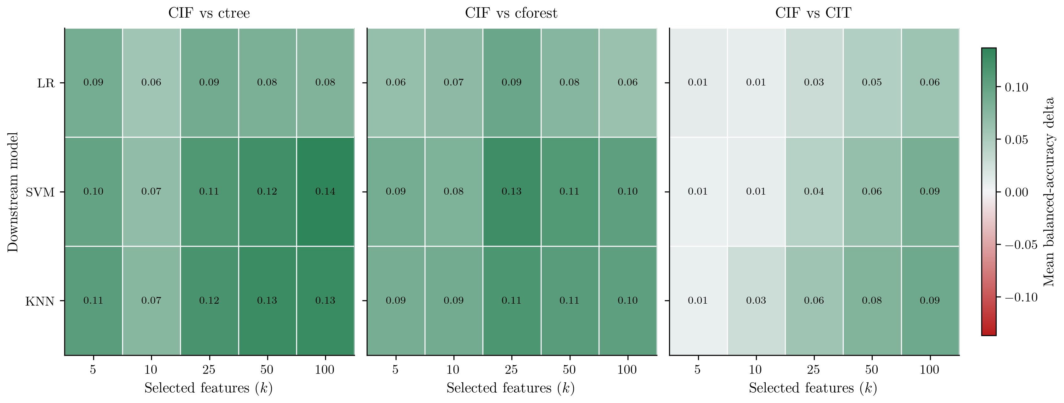

For the seed checks, each method is ranked separately within each fixed seed. Keeping only datasets with results for every method, downstream learner, standard top-\(k\) value, and seed leaves 12 classification datasets and 6 regression datasets complete across all five seeds. These tables summarize seed variation by rank without intervals or tests. In these tables, a seed column is the method’s ordinal position after sorting that seed’s averaged dataset-level ranks, while mean rank is the averaged dataset-level rank value itself. Rows follow the main benchmark order.
| Method | Seed 1 | Seed 2 | Seed 3 | Seed 4 | Seed 5 | Mean position | Mean rank | ||||||||||||||||||||||||||||||||||||||||||||||||||||||||||||||||||||||||||||||||||||||||||||||||||||||||||||||||||||||||||||||
|---|---|---|---|---|---|---|---|---|---|---|---|---|---|---|---|---|---|---|---|---|---|---|---|---|---|---|---|---|---|---|---|---|---|---|---|---|---|---|---|---|---|---|---|---|---|---|---|---|---|---|---|---|---|---|---|---|---|---|---|---|---|---|---|---|---|---|---|---|---|---|---|---|---|---|---|---|---|---|---|---|---|---|---|---|---|---|---|---|---|---|---|---|---|---|---|---|---|---|---|---|---|---|---|---|---|---|---|---|---|---|---|---|---|---|---|---|---|---|---|---|---|---|---|---|---|---|---|---|---|---|---|---|---|
| LightGBM | 2 | 1 | 2 | 1 | 1 | 1.4 | 4.7 | ||||||||||||||||||||||||||||||||||||||||||||||||||||||||||||||||||||||||||||||||||||||||||||||||||||||||||||||||||||||||||||||
| XGBoost | 1 | 3 | 1 | 2 | 2 | 1.8 | 5.0 | ||||||||||||||||||||||||||||||||||||||||||||||||||||||||||||||||||||||||||||||||||||||||||||||||||||||||||||||||||||||||||||||
| CatBoost | 3 | 2 | 5 | 3 | 4 | 3.4 | 5.7 | ||||||||||||||||||||||||||||||||||||||||||||||||||||||||||||||||||||||||||||||||||||||||||||||||||||||||||||||||||||||||||||||
| CIF | 5 | 5 | 4 | 4 | 7 | 5.0 | 6.1 | ||||||||||||||||||||||||||||||||||||||||||||||||||||||||||||||||||||||||||||||||||||||||||||||||||||||||||||||||||||||||||||||
| RF | 4 | 4 | 3 | 6 | 3 | 4.0 | 6.0 | ||||||||||||||||||||||||||||||||||||||||||||||||||||||||||||||||||||||||||||||||||||||||||||||||||||||||||||||||||||||||||||||
| RF-RFE | 7 | 7 | 7 | 5 | 6 | 6.4 | 7.2 | ||||||||||||||||||||||||||||||||||||||||||||||||||||||||||||||||||||||||||||||||||||||||||||||||||||||||||||||||||||||||||||||
| ExtraTrees | 6 | 6 | 6 | 7 | 5 | 6.0 | 6.5 | ||||||||||||||||||||||||||||||||||||||||||||||||||||||||||||||||||||||||||||||||||||||||||||||||||||||||||||||||||||||||||||||
| DT | 8 | 9 | 9 | 8 | 8 | 8.4 | 8.5 | ||||||||||||||||||||||||||||||||||||||||||||||||||||||||||||||||||||||||||||||||||||||||||||||||||||||||||||||||||||||||||||||
| RT | 11 | 10 | 12 | 12 | 11 | 11.2 | 10.0 | ||||||||||||||||||||||||||||||||||||||||||||||||||||||||||||||||||||||||||||||||||||||||||||||||||||||||||||||||||||||||||||||
| CIT | 10 | 11 | 10 | 10 | 10 | 10.2 | 9.7 | ||||||||||||||||||||||||||||||||||||||||||||||||||||||||||||||||||||||||||||||||||||||||||||||||||||||||||||||||||||||||||||||
| Boruta | 9 | 8 | 8 | 9 | 9 | 8.6 | 8.4 | ||||||||||||||||||||||||||||||||||||||||||||||||||||||||||||||||||||||||||||||||||||||||||||||||||||||||||||||||||||||||||||||
| MC filter | 12 | 12 | 11 | 11 | 12 | 11.6 | 10.4 | ||||||||||||||||||||||||||||||||||||||||||||||||||||||||||||||||||||||||||||||||||||||||||||||||||||||||||||||||||||||||||||||
| PI | 16 | 16 | 16 | 16 | 16 | 16.0 | 13.1 | ||||||||||||||||||||||||||||||||||||||||||||||||||||||||||||||||||||||||||||||||||||||||||||||||||||||||||||||||||||||||||||||
| cforest | 15 | 15 | 15 | 14 | 15 | 14.8 | 12.6 | ||||||||||||||||||||||||||||||||||||||||||||||||||||||||||||||||||||||||||||||||||||||||||||||||||||||||||||||||||||||||||||||
| RDC filter | 13 | 13 | 13 | 13 | 13 | 13.0 | 11.5 | ||||||||||||||||||||||||||||||||||||||||||||||||||||||||||||||||||||||||||||||||||||||||||||||||||||||||||||||||||||||||||||||
| ctree | 14 | 14 | 14 | 15 | 14 | 14.2 | 12.5 | ||||||||||||||||||||||||||||||||||||||||||||||||||||||||||||||||||||||||||||||||||||||||||||||||||||||||||||||||||||||||||||||
| CPI | 17 | 17 | 17 | 17 | 17 | 17.0 | 15.3 |
4pt
| Method | Seed 1 | Seed 2 | Seed 3 | Seed 4 | Seed 5 | Mean position | Mean rank | ||||||||||||||||||||||||||||||||||||||||||||||||||||||||||||||||||||||||||||||||||||||||||||||||||||||||||||||||||||||||||||||
|---|---|---|---|---|---|---|---|---|---|---|---|---|---|---|---|---|---|---|---|---|---|---|---|---|---|---|---|---|---|---|---|---|---|---|---|---|---|---|---|---|---|---|---|---|---|---|---|---|---|---|---|---|---|---|---|---|---|---|---|---|---|---|---|---|---|---|---|---|---|---|---|---|---|---|---|---|---|---|---|---|---|---|---|---|---|---|---|---|---|---|---|---|---|---|---|---|---|---|---|---|---|---|---|---|---|---|---|---|---|---|---|---|---|---|---|---|---|---|---|---|---|---|---|---|---|---|---|---|---|---|---|---|---|
| ExtraTrees | 2 | 1 | 1 | 2 | 2 | 1.6 | 6.8 | ||||||||||||||||||||||||||||||||||||||||||||||||||||||||||||||||||||||||||||||||||||||||||||||||||||||||||||||||||||||||||||||
| CatBoost | 1 | 6 | 3 | 1 | 1 | 2.4 | 6.9 | ||||||||||||||||||||||||||||||||||||||||||||||||||||||||||||||||||||||||||||||||||||||||||||||||||||||||||||||||||||||||||||||
| CIF | 5 | 5 | 5 | 4 | 6 | 5.0 | 7.9 | ||||||||||||||||||||||||||||||||||||||||||||||||||||||||||||||||||||||||||||||||||||||||||||||||||||||||||||||||||||||||||||||
| RF | 4 | 3 | 4 | 6 | 5 | 4.4 | 8.0 | ||||||||||||||||||||||||||||||||||||||||||||||||||||||||||||||||||||||||||||||||||||||||||||||||||||||||||||||||||||||||||||||
| RT | 3 | 2 | 2 | 5 | 4 | 3.2 | 7.6 | ||||||||||||||||||||||||||||||||||||||||||||||||||||||||||||||||||||||||||||||||||||||||||||||||||||||||||||||||||||||||||||||
| DT | 11 | 4 | 7 | 3 | 3 | 5.6 | 8.1 | ||||||||||||||||||||||||||||||||||||||||||||||||||||||||||||||||||||||||||||||||||||||||||||||||||||||||||||||||||||||||||||||
| LightGBM | 7 | 8 | 8 | 8 | 7 | 7.6 | 8.7 | ||||||||||||||||||||||||||||||||||||||||||||||||||||||||||||||||||||||||||||||||||||||||||||||||||||||||||||||||||||||||||||||
| RDC filter | 12 | 11 | 9 | 12 | 11 | 11.0 | 9.8 | ||||||||||||||||||||||||||||||||||||||||||||||||||||||||||||||||||||||||||||||||||||||||||||||||||||||||||||||||||||||||||||||
| CIT | 8 | 9 | 12 | 10 | 13 | 10.4 | 9.4 | ||||||||||||||||||||||||||||||||||||||||||||||||||||||||||||||||||||||||||||||||||||||||||||||||||||||||||||||||||||||||||||||
| PC filter | 13 | 13 | 13 | 13 | 12 | 12.8 | 10.5 | ||||||||||||||||||||||||||||||||||||||||||||||||||||||||||||||||||||||||||||||||||||||||||||||||||||||||||||||||||||||||||||||
| DC filter | 15 | 15 | 14 | 15 | 14 | 14.6 | 11.1 | ||||||||||||||||||||||||||||||||||||||||||||||||||||||||||||||||||||||||||||||||||||||||||||||||||||||||||||||||||||||||||||||
| XGBoost | 6 | 7 | 10 | 7 | 8 | 7.6 | 8.8 | ||||||||||||||||||||||||||||||||||||||||||||||||||||||||||||||||||||||||||||||||||||||||||||||||||||||||||||||||||||||||||||||
| Boruta | 10 | 12 | 11 | 11 | 9 | 10.6 | 9.7 | ||||||||||||||||||||||||||||||||||||||||||||||||||||||||||||||||||||||||||||||||||||||||||||||||||||||||||||||||||||||||||||||
| PI | 9 | 10 | 6 | 9 | 10 | 8.8 | 9.1 | ||||||||||||||||||||||||||||||||||||||||||||||||||||||||||||||||||||||||||||||||||||||||||||||||||||||||||||||||||||||||||||||
| RF-RFE | 14 | 14 | 15 | 14 | 15 | 14.4 | 10.9 | ||||||||||||||||||||||||||||||||||||||||||||||||||||||||||||||||||||||||||||||||||||||||||||||||||||||||||||||||||||||||||||||
| cforest | 16 | 17 | 16 | 16 | 17 | 16.4 | 12.3 | ||||||||||||||||||||||||||||||||||||||||||||||||||||||||||||||||||||||||||||||||||||||||||||||||||||||||||||||||||||||||||||||
| ctree | 18 | 18 | 18 | 17 | 18 | 17.8 | 13.1 | ||||||||||||||||||||||||||||||||||||||||||||||||||||||||||||||||||||||||||||||||||||||||||||||||||||||||||||||||||||||||||||||
| CPI | 17 | 16 | 17 | 18 | 16 | 16.8 | 12.3 |
4pt
16 Feature use in sampled forests↩︎
The extended \(p\)-sweep expands the main-text feature-sampling analysis, separate from the benchmark-stability summaries in 15. [fig:candidate-dimension-curves,fig:regression-candidate-dimension-curves] show feature-sampling results for \(p \in \{100,500,1{,}000\}\). Each forest uses 1,000 trees, with classification and regression shown separately. For each method and feature dimension \(p\), each point is the mean over \(n_{\mathrm{informative}} \in \{1,2,5,10\}\), and the capped bar spans the minimum and maximum over those four sparse settings.
In classification, evaluating all nonconstant features at each split gives the largest informative-feature gains in sparse high-\(p\) settings. CIF-all keeps feature muting and the other tree settings unchanged while removing feature subsampling. With two informative features and \(p{=}100\), CIF uses informative features in 40.0% of splits, while CIF-all does so in 100.0%. The corresponding values are 12.2% versus 90.2% at \(p{=}500\) and 9.0% versus 100.0% at \(p{=}1{,}000\). CIF-all also uses 70, 264, and 439 fewer distinct uninformative features than CIF. With five informative features, the CIF-all minus CIF differences are 25.1, 56.4, and 54.3 percentage points at \(p{=}100\), \(p{=}500\), and \(p{=}1{,}000\).
Regression shows a similar informative-feature use pattern in the one- and two-informative-feature settings, and CIF-all also uses more distinct uninformative features. With two informative features and \(p{=}100\), CIF uses informative features in 39.9% of splits, while CIF-all does so in 58.8%. The corresponding values are 19.7% versus 46.7% at \(p{=}500\) and 11.6% versus 35.9% at \(p{=}1{,}000\). With one informative feature, the CIF-all minus CIF differences are 29.8, 18.9, and 42.1 percentage points.