Fredholm–residue selection of the unsteady Kutta amplitude
July 01, 2026
Abstract
We give an operator-theoretic interpretation of unsteady Kutta selection in trailing-edge acoustic receptivity. The inviscid acoustic–wake problem leaves one outgoing wake amplitude undetermined. We show that, under explicit structural hypotheses, this amplitude is the same scalar obtained from three representations: cancellation of the inverse-square-root edge singularity, Fredholm compatibility of the viscous lower-deck problem, and the residue of the Kutta-normalized transform solution at the downstream wake pole: \(\displaystyle A = -\frac{C_-^{(0)}}{C_-^{(KH)}} = -\frac{\langle \mathbf{F}_{\rm inc},\Psi^\ast\rangle}{\langle \mathbf{F}_{KH},\Psi^\ast\rangle} = i\operatorname*{Res}_{\alpha=\alpha_{KH}}\mathcal{M}(\alpha)\). The inner Fredholm–edge mechanism is verified exactly in a linear-shear lower-deck model, where the primal shear and adjoint velocity are Airy fields and the edge concomitant is nonzero outside a discrete resonance set.
unsteady Kutta selection , trailing-edge receptivity , viscous–inviscid matching , triple-deck theory , Fredholm compatibility , Wiener–Hopf method , wake-pole residue.
76G25, 76D10, 35Q35, 47A53, 35C15, 35C20
1 Introduction and main identity↩︎
The unsteady Kutta condition is a singular selection principle at a sharp edge. In steady inviscid airfoil theory it fixes the circulation by removing the inverse-square-root velocity singularity at the trailing edge. In unsteady acoustic receptivity the situation is subtler: the outer acoustic–wake problem may admit an outgoing hydrodynamic wake mode, and the inviscid equations alone then leave one complex amplitude undetermined. This paper formulates that missing scalar as a Fredholm compatibility condition for the viscous lower-deck problem and identifies the same scalar with the pole residue of a Kutta-normalized transform solution. The structural hypotheses under which the identification holds are isolated and then verified in closed form for the canonical linear-shear model of the unsteady lower deck, for which the adjoint state is an Airy-derivative field and the edge concomitant is computable.
That a Kutta condition in unsteady flow need not coincide with its steady form, and that its applicability is itself a question, was surveyed in [1]–[5]. The vortex-sheet-from-an-edge problem and its sensitivity to the choice of edge condition were analyzed in [6]–[14] and the monograph of Howe [15], [16]. The viscous justification of the steady Kutta condition through triple-deck theory originates in [17]–[25]; the unsteady and oscillating-edge viscous structure was studied by Brown & Daniels [26], Daniels [27], [28], and Brown & Stewartson [29]. Boundary-layer receptivity to sound, in which an inviscid amplitude is fixed by an edge or solvability mechanism, is reviewed in [30]–[40]. The linearized unsteady lower deck about a uniform shear was solved exactly by Terent’ev in the vibrating-ribbon problem [41]; the worked example of Section 4 is its trailing-edge (plate–wake switching) analogue. The downstream/upstream classification of spatial poles we invoke is the Briggs–Bers criterion [42]–[52]. The transform analysis rests on the Wiener–Hopf technique [53], [54]; for finite-angle edges it is replaced by Mellin and functional-difference methods for wedges [14], [55]–[58]. The contribution here is to tie the inner (viscous, Fredholm) and outer (transform, residue) selections together into a single conditional identity, with all structural hypotheses isolated, and to exhibit a model in which the inner hypotheses are theorems. The main contribution is not a full viscous proof for the physical trailing-edge base flow. Rather, it is a closed applied-mathematical selection mechanism: under explicitly stated structural hypotheses, the unsteady Kutta amplitude is the same scalar in three representations, namely the outer edge-regularity quotient, the lower-deck adjoint Fredholm quotient, and the downstream pole residue (1, 2). The inner part of this mechanism is then verified in closed form for the canonical linear-shear lower-deck model (10).
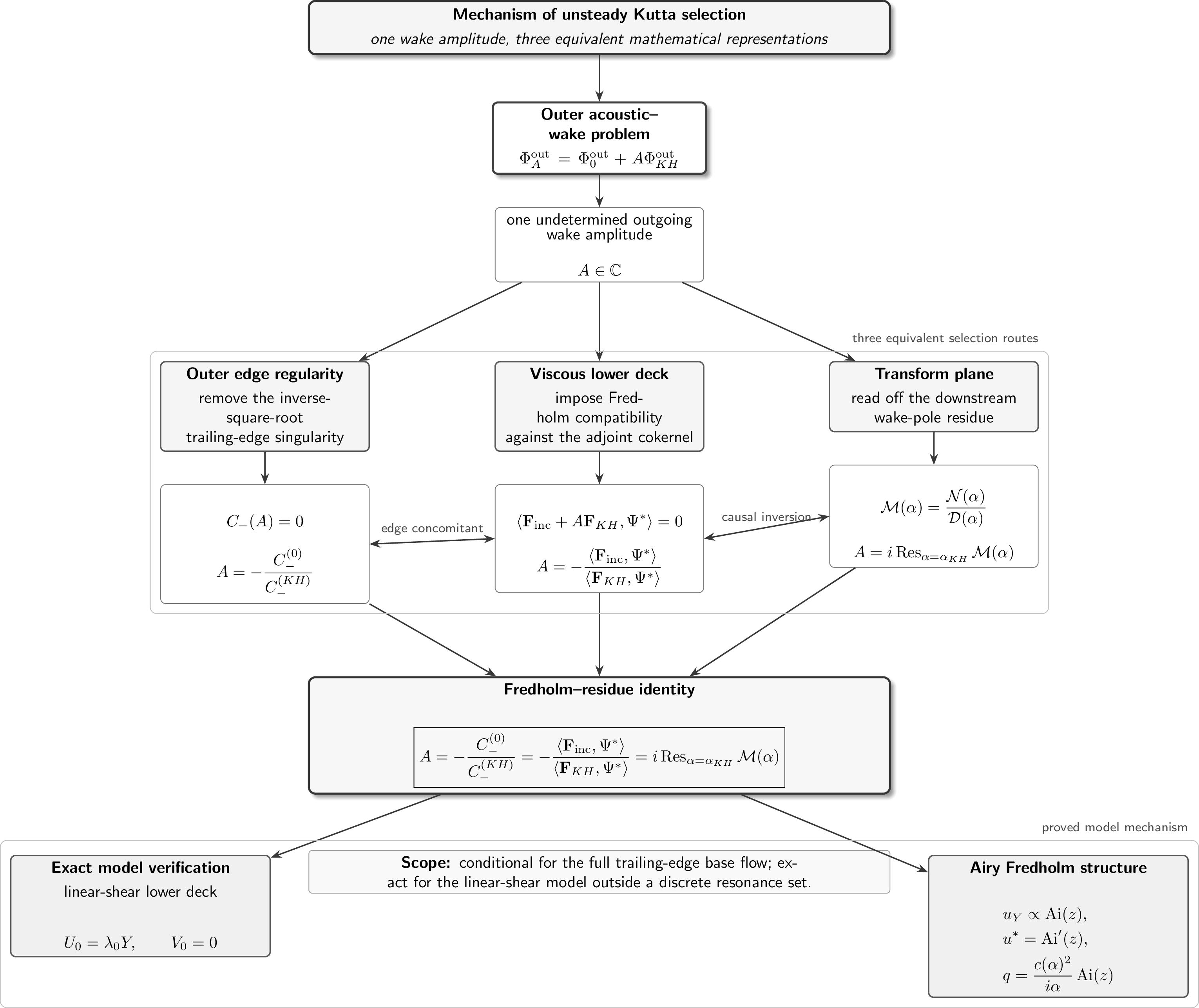
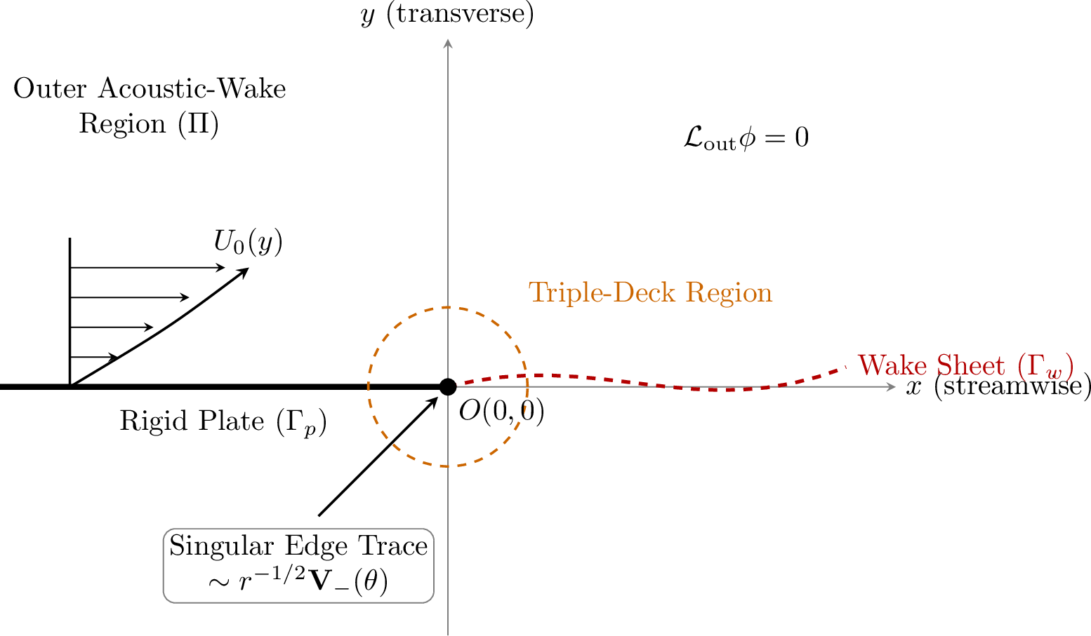
Let \[\Gamma_p=(-\infty,0)\times\{0\},\qquad \Gamma_w=(0,\infty)\times\{0\},\qquad \Pi=\mathbb{R}^2\setminus(\Gamma_p\cup\Gamma_w),\] and let \(O=(0,0)\). We use \(e^{-i\omega_{\rm phys}t}\), set \[M=\frac{U}{c}\in(0,1),\qquad \beta=(1-M^2)^{1/2},\qquad k_0=\frac{\omega_{\rm phys}}{c},\qquad k=\frac{\omega_{\rm phys}L}{U},\] and write \(\phi=\phi^{\rm inc}+\phi^{\rm sc}\). Two length scales are in play and must be kept distinct. The outer acoustic–wake problem 1 –2 is posed on the hydrodynamic length \(\ell_\omega=U/\omega_{\rm phys}\), on which the Helmholtz number \(k_0\ell_\omega=M\) is \(\mathcal{O}(1)\) uniformly in the Reynolds number; the chord \(L\) enters only through \(Re\) and the triple-deck scalings of 3. All outer coordinates \((x,y)\) below are measured on \(\ell_\omega\); the intermediate matching between this outer field and the lower deck is part of the matching map \(\mathcal{M}_{\mathrm{in}}\) introduced in 26 (for the hierarchy of unsteady regions see [26], [28]). In the outer region, \[\label{eq:intro-Lout} \mathcal{L}_{\mathrm{out}}\phi=0,\qquad \mathcal{L}_{\mathrm{out}}:=\beta^2\partial_x^2+\partial_y^2 +2iMk_0\partial_x+k_0^2 .\tag{1}\] On \(\Gamma_p\), \(\gamma_p^\pm\partial_y\phi=0\). On \(\Gamma_w\), instead of imposing a degenerate equal-speed convected-sheet closure, we use an abstract inviscid-sheet transmission law \[\mathcal{T}_{\mathrm{sh}}(\omega_{\rm phys},\mathcal{G}) \begin{pmatrix} \gamma_w^+\phi\\ \gamma_w^-\phi\\ \gamma_w^+\partial_y\phi\\ \gamma_w^-\partial_y\phi\\ \eta \end{pmatrix}=0,\qquad x>0 .\] Here \(\eta(x)e^{-i\omega_{\rm phys}t}\) is the sheet displacement and \(\mathcal{G}\) denotes the edge geometry, acoustic incidence, and base sheet data. The equal-speed relations \[\partial_y\phi^\pm=(-i\omega_{\rm phys}+U\partial_x)\eta,\qquad (-i\omega_{\rm phys}+U\partial_x)[\phi]=0\] are only a neutral limiting model; the downstream instability below belongs to the full operator \(\mathcal{T}_{\mathrm{sh}}\). We write the outgoing outer problem as \[\label{eq:intro-Aout} \mathcal{A}_{\mathrm{out}}(\omega_{\rm phys},\mathcal{G})\Phi=\mathcal{F}_{\mathrm{out}}^{\rm inc},\qquad \Phi=(\phi,\eta).\tag{2}\] For a homogeneous normal mode \(\Phi(x,y)=e^{i\alpha x} \big(\varphi^+(y),\varphi^-(y),\eta_0\big)\), one obtains \[(\varphi^\pm)''-\mu(\alpha)^2\varphi^\pm=0,\qquad \mu(\alpha)^2=\beta^2\alpha^2+2Mk_0\alpha-k_0^2 ,\] with the outgoing branch of \(\mu\). The sheet law reduces the normal-mode problem to \[\mathcal{B}(\alpha;\omega_{\rm phys},\mathcal{G})\mathbf{a}=0,\qquad \mathcal{D}(\alpha;\omega_{\rm phys},\mathcal{G}):= \det\mathcal{B}(\alpha;\omega_{\rm phys},\mathcal{G}).\] We assume a simple downstream wake pole \[\mathcal{D}(\alpha_{KH};\omega_{\rm phys},\mathcal{G})=0,\qquad \partial_\alpha\mathcal{D}(\alpha_{KH};\omega_{\rm phys},\mathcal{G})\neq0,\qquad \Im\alpha_{KH}<0 .\] With \(e^{i\alpha x-i\omega_{\rm phys}t}\), the last inequality corresponds to downstream spatial growth (a convective spatial instability; see the causal deformation of 5.3). The associated outgoing homogeneous field is \(\displaystyle \Phi_{KH}^{\rm out}=(\phi_{KH}^{\rm out},\eta_{KH})\), normalized once and for all by the wake functional \(\ell_{KH}\) of 10 , \(\ell_{KH}(\Phi_{KH}^{\rm out})=1\). The first structural hypothesis is the one-dimensional kernel \(\displaystyle \ker\mathcal{A}_{\mathrm{out}}^{\rm hom} = \mathop{\mathrm{span}}\{\Phi_{KH}^{\rm out}\}\). Thus every outgoing forced outer field has the affine form \[\label{eq:intro-outer-family} \Phi_A^{\rm out} = \Phi_0^{\rm out}+A\Phi_{KH}^{\rm out},\qquad A\in\mathbb{C} .\tag{3}\] The unknown scalar \(A\) is the receptivity amplitude. Near \(O\), let \((r,\theta)\) denote polar coordinates after the local stretching \((x,y)\mapsto(x/\beta,y)\), \(-\pi<\theta<\pi\). We assume the standard slit-plane edge pencil has first nonconstant indicial root \(\lambda=1/2\). Hence \[\nabla\phi_A^{\rm out} = C_-(A)r^{-1/2}\mathbf{V}_{-}(\theta)+\mathcal{O}(1), \qquad \mathbf{V}_{-}(\theta)=\frac{1}{2}\Psi_-(\theta)e_r+\Psi_-'(\theta)e_\theta, \qquad \Psi_-(\theta)=\sin\frac{\theta}{2}.\] By linearity, \(C_-(A)=C_-^{(0)}+A C_-^{(KH)}\). The outer regularity form of the Kutta condition is \(C_-(A)=0\). If \(C_-^{(KH)}\neq0\), this condition alone gives \(\displaystyle A=-\frac{C_-^{(0)}}{C_-^{(KH)}}\). The central question is why this inviscid regularity condition is selected by the viscous trailing-edge structure. For the lower-deck scaling, set \[Re=\frac{UL}{\nu},\qquad \varepsilon=Re^{-1/8},\qquad x=\varepsilon^3L\,X,\qquad y=\varepsilon^5L\,Y,\qquad T=\frac{Ut}{\varepsilon^2L}.\] Then \[e^{-i\omega_{\rm phys}t}=e^{-i\Omega T},\qquad \Omega=\frac{\omega_{\rm phys}\varepsilon^2L}{U} = \varepsilon^2k = Re^{-1/4}k .\] Thus the distinguished unsteady triple-deck regime is \(\Omega=\mathcal{O}(1)\) with \(k=\mathcal{O}(Re^{1/4})\). Linearization of the unsteady lower deck about a steady base state gives \(\mathcal{L}_{\mathrm{TD}}(\Omega)W=F\), where \(W=(u,v,p,a)^{\mathsf T}\). The outer-to-inner matching data generated by 3 split as \[F_{\rm match}(A) = C_-(A)\mathbf{F}_{\mathrm{sing}}+\mathbf{F}_{\mathrm{inc}}(\Omega)+A\mathbf{F}_{KH}(\Omega), \qquad \mathbf{F}_{\mathrm{sing}}\in\mathcal{E}_{\mathrm{edge}},\quad \mathbf{F}_{\mathrm{inc}}+A\mathbf{F}_{KH}\in\mathcal{H}_\sigma,\] where \(\mathcal{E}_{\mathrm{edge}}=\mathop{\mathrm{span}}\{r^{-1/2}\mathbf{V}_{-}\}\) is the singular edge-trace space; its lower-deck realization is an \(|X|^{-1/2}\) line datum in the matching and pressure–displacement components, and as such it does not belong to the regular data space \(\mathcal{H}_\sigma\) (2). Solvability in the bounded graph domain therefore requires \[\Pi_{\rm sing}F_{\rm match}(A)=0 \quad\Longleftrightarrow\quad C_-(A)=0 .\] The Fredholm realization is a closed densely defined operator \(\displaystyle \mathcal{L}_{\mathrm{TD}}(\Omega):\mathcal{X}_\sigma\to\mathcal{H}_\sigma\) between the weighted spaces of 3.4, whose downstream weight is chosen so that the inner counterpart of the shed wake mode belongs to the domain (Remark 5). We assume \[\mathop{\mathrm{ind}}\mathcal{L}_{\mathrm{TD}}(\Omega)=0,\qquad \ker\mathcal{L}_{\mathrm{TD}}(\Omega)^\ast=\mathop{\mathrm{span}}\{\Psi^\ast(\Omega)\},\qquad \langle\mathbf{F}_{KH}(\Omega),\Psi^\ast(\Omega)\rangle_{\mathcal{H}_\sigma}\neq0.\] The regular Fredholm condition is \[\mathbf{F}_{\mathrm{inc}}(\Omega)+A\mathbf{F}_{KH}(\Omega)\in\mathop{\mathrm{Ran}}\mathcal{L}_{\mathrm{TD}}(\Omega) \quad\Longleftrightarrow\quad \langle\mathbf{F}_{\mathrm{inc}}(\Omega)+A\mathbf{F}_{KH}(\Omega),\Psi^\ast(\Omega)\rangle_{\mathcal{H}_\sigma}=0 .\] The edge trace and the regular Fredholm projection are linked by the consistency relation \[\label{eq:intro-KF-consistency} \langle\mathbf{F}_{\mathrm{inc}}(\Omega)+A\mathbf{F}_{KH}(\Omega),\Psi^\ast(\Omega)\rangle_{\mathcal{H}_\sigma} = \chi(\Omega)C_-(A),\qquad \chi(\Omega)\neq0 .\tag{4}\] This is not an independent hypothesis: in 3 (Proposition 7, Eq. 40 ) it is derived from the Green identity of Appendix 7 together with the augmented solvability of (H3) below, with \(\chi(\Omega)=-\kappa(\Omega)\); it thus reduces to nondegeneracy of the edge concomitant, \(\kappa(\Omega)\neq0\). Equivalently, \(\displaystyle C_-(A)=0\) iff \(\displaystyle \mathbf{F}_{\mathrm{inc}}(\Omega)+A\mathbf{F}_{KH}(\Omega)\in\mathop{\mathrm{Ran}}\mathcal{L}_{\mathrm{TD}}(\Omega)\). The same relation can be expressed through the finite edge concomitant \[\mathscr{B}_{\mathrm{edge}}:\mathcal{E}_{\mathrm{edge}}\times\ker\mathcal{L}_{\mathrm{TD}}(\Omega)^\ast\to\mathbb{C},\qquad \mathscr{B}_{\mathrm{edge}}(C_-(A)r^{-1/2}\mathbf{V}_{-},\Psi^\ast)=C_-(A)\kappa(\Omega),\] with \(\displaystyle \kappa(\Omega)=\mathscr{B}_{\mathrm{edge}}(r^{-1/2}\mathbf{V}_{-},\Psi^\ast(\Omega))\neq0\). Thus the singular edge cancellation and the Fredholm projection vanish for the same value of \(A\). The transform formulation gives an independent representation of that same value. In the flat-plate case, the Kutta-normalized Wiener–Hopf solution is assumed meromorphic near \(\alpha_{KH}\), i.e., \(\displaystyle \mathcal{M}(\alpha;\Omega,\mathcal{G}) = \frac{\mathcal{N}(\alpha;\Omega,\mathcal{G})}{\mathcal{D}(\alpha;\Omega,\mathcal{G})}\). With the wake normalization \(\ell_{KH}\) of 10 , the coefficient of the downstream wake mode is the residue at \(\alpha_{KH}\) multiplied by the explicit contour-orientation factor \(i\) of 63 . For finite-angle wedges with self-similar sheet data, the Fourier representation is replaced by a Mellin representation \[\mathcal{M}_{\rm wedge}(s;\Omega,\mathcal{G}) = \frac{\mathcal{N}_{\rm wedge}(s;\Omega,\mathcal{G})}{\mathcal{D}_{\rm wedge}(s;\Omega,\mathcal{G})}, \qquad A_{\mathrm{rec}}^{\rm wedge} = \mathop{\mathrm{Res}}_{s=s_{KH}}\mathcal{M}_{\rm wedge}(s;\Omega,\mathcal{G}),\] see Assumption 4. We now state the main result (Figure 2).
Theorem 1 (Fredholm–residue identity for the unsteady Kutta amplitude). Assume the following hypotheses:
\(\ker\mathcal{A}_{\mathrm{out}}^{\rm hom}=\mathop{\mathrm{span}}\{\Phi_{KH}^{\rm out}\}\), \(\mathcal{D}(\alpha_{KH};\omega_{\rm phys},\mathcal{G})=0\), \(\mathcal{D}_\alpha(\alpha_{KH};\omega_{\rm phys},\mathcal{G})\neq0\), \(\Im\alpha_{KH}<0\);
\(\nabla\phi_A^{\rm out}=C_-(A)r^{-1/2}\mathbf{V}_{-}+\mathcal{O}(1)\), \(C_-(A)=C_-^{(0)}+AC_-^{(KH)}\), \(C_-^{(KH)}\neq0\);
\(\mathcal{L}_{\mathrm{TD}}(\Omega):\mathcal{X}_\sigma\to\mathcal{H}_\sigma\) is Fredholm of index \(0\), \(\ker\mathcal{L}_{\mathrm{TD}}(\Omega)^\ast=\mathop{\mathrm{span}}\{\Psi^\ast(\Omega)\}\), and for every \(A\in\mathbb{C}\) the matching problem is solvable in the augmented class \(\mathcal{D}_{\mathrm{match}}=\mathcal{E}_{\mathrm{edge}}\oplus\mathcal{H}_\sigma\);
\(\kappa(\Omega)=\mathscr{B}_{\mathrm{edge}}(r^{-1/2}\mathbf{V}_{-},\Psi^\ast(\Omega))\neq0\) (with (H2)–(H3) this implies \(\langle\mathbf{F}_{KH},\Psi^\ast\rangle\neq0\) and 4 with \(\chi=-\kappa\));
\(\mathcal{M}(\alpha;\Omega,\mathcal{G})=\mathcal{N}(\alpha;\Omega,\mathcal{G})/ \mathcal{D}(\alpha;\Omega,\mathcal{G})\) is the Kutta-normalized meromorphic transform response near \(\alpha_{KH}\).
Then bounded viscous–inviscid matching selects a unique amplitude \[A_{\mathrm{rec}}(\Omega,\mathcal{G}) = -\frac{C_-^{(0)}}{C_-^{(KH)}} = -\frac{ \langle \mathbf{F}_{\mathrm{inc}}(\Omega),\Psi^\ast(\Omega)\rangle_{\mathcal{H}_\sigma}}{ \langle \mathbf{F}_{KH}(\Omega),\Psi^\ast(\Omega)\rangle_{\mathcal{H}_\sigma}} = i\mathop{\mathrm{Res}}_{\alpha=\alpha_{KH}} \mathcal{M}(\alpha;\Omega,\mathcal{G}),\] the last equality holding for the wake normalization \(\ell_{KH}(\Phi_{KH}^{\rm out})=1\) of 10 . If \(\alpha_{KH}\) is simple, then \(\displaystyle A_{\mathrm{rec}}(\Omega,\mathcal{G}) = \frac{i\,\mathcal{N}(\alpha_{KH};\Omega,\mathcal{G})}{\partial_\alpha\mathcal{D}(\alpha_{KH};\Omega,\mathcal{G})}\). Equivalently, \(\displaystyle C_-(A)=0\) iff \(\displaystyle \Pi_{\rm sing}F_{\rm match}(A)=0\) iff \(\displaystyle \langle\mathbf{F}_{\mathrm{inc}}+A\mathbf{F}_{KH},\Psi^\ast\rangle_{\mathcal{H}_\sigma}=0\) iff \(\displaystyle \mathbf{F}_{\mathrm{inc}}+A\mathbf{F}_{KH}\in\mathop{\mathrm{Ran}}\mathcal{L}_{\mathrm{TD}}(\Omega)\). For a finite-angle wedge satisfying the analogous Mellin hypotheses, including the self-similarity Assumption 4, \(\displaystyle A_{\mathrm{rec}}^{\rm wedge}(\Omega,\mathcal{G}) = -\frac{ \langle \mathbf{F}_{\mathrm{inc}}^{\rm wedge},\Psi_{\rm wedge}^\ast\rangle_{\mathcal{H}_\sigma}}{ \langle \mathbf{F}_{KH}^{\rm wedge},\Psi_{\rm wedge}^\ast\rangle_{\mathcal{H}_\sigma}} = \mathop{\mathrm{Res}}_{s=s_{KH}} \mathcal{M}_{\rm wedge}(s;\Omega,\mathcal{G})\).
Proof at the structural level. By (H1), every outgoing forced outer solution is \(\Phi_A^{\rm out}=\Phi_0^{\rm out}+A\Phi_{KH}^{\rm out}\). By (H2), its singular edge trace is \(C_-(A)r^{-1/2}\mathbf{V}_{-}\). Since bounded lower-deck matching has data in \(\mathcal{H}_\sigma\) and the singular line datum is excluded from \(\mathcal{H}_\sigma\) by Lemma 2, the \(\mathcal{E}_{\mathrm{edge}}\)-component of \(F_{\rm match}(A)\) must vanish; hence \(C_-(A)=0\), which gives \(A=-C_-^{(0)}/C_-^{(KH)}\). By (H3), the regular problem is solvable exactly when the Fredholm projection against \(\Psi^\ast\) vanishes. By (H3)–(H4) and Proposition 7, that Fredholm projection equals \(-\kappa(\Omega)C_-(A)\), so the Fredholm-selected and Kutta-selected amplitudes coincide, giving the adjoint quotient. Finally, by (H5) and uniqueness of the Kutta-normalized outer field, the transform solution has the same amplitude; the causal inverse-transform deformation of 5.3 identifies this coefficient, in the normalization \(\ell_{KH}(\Phi_{KH}^{\rm out})=1\), with \(i\) times the residue at \(\alpha_{KH}\). The simple-pole formula is the Laurent coefficient of \(\mathcal{N}/\mathcal{D}\). ◻
The theorem is conditional in the following explicit places: \[\text{simple outgoing wake pole},\qquad \text{edge indicial root }\lambda=1/2,\] \[\text{Fredholm lower-deck realization with augmented solvability},\] \[\text{nonzero edge concomitant},\qquad \text{meromorphic Kutta-normalized transform}.\] Figure 1 shows the flowchart of our model. [sec:outer,sec:inner] develop each object and prove the algebraic implications; 4 verifies the inner hypotheses (H3)–(H4) in closed form for the linear-shear model, where the adjoint state is an Airy-derivative field, the Wiener–Hopf kernel and wake pole are explicit, and \(\kappa(\Omega)\neq0\) off a discrete resonance set; 5 gives the transform representation and pole-residue formulae; 6 discusses scope and limitations; Appendix 7 derives the formal adjoint and edge concomitant; and Appendix 8 outlines the Mellin analogue for finite-angle wedges.
None
Figure 2: The selection mechanism of 1: the unsteady Kutta amplitude is the same scalar in three representations. The equivalences are 9 and 16; the nondegeneracies making them equivalences are (H2)–(H4)..
2 Outer acoustic–wake problem and the edge obstruction↩︎
Let \[\Gamma_p=(-\infty,0)\times\{0\},\qquad \Gamma_w=(0,\infty)\times\{0\},\qquad \Pi=\mathbb{R}^2\setminus(\Gamma_p\cup\Gamma_w).\] The edge is \(O=(0,0)\). The incident acoustic field is denoted by \(\phi^{\rm inc}\); the total outer potential is \[\phi=\phi^{\rm inc}+\phi^{\rm sc},\qquad \phi^\pm(x)=\lim_{y\to0^\pm}\phi(x,y).\] We use the convention \(e^{-i\omega_{\rm phys}t}\), and write \[M=\frac{U}{c}\in(0,1),\qquad \beta=(1-M^2)^{1/2},\qquad k_0=\frac{\omega_{\rm phys}}{c},\qquad k=\frac{\omega_{\rm phys}L}{U}.\] As stated in 1, the outer coordinates are measured on the hydrodynamic length \(\ell_\omega=U/\omega_{\rm phys}\), so that the outer problem is uniformly \(\mathcal{O}(1)\) in \(Re\) throughout the distinguished regime 18 . The physical configuration of the problem is illustrated in Figure 3, which consists of a semi-infinite rigid plate (\(\Gamma_p\)) and a downstream wake sheet (\(\Gamma_w\)).
2.1 Convected Helmholtz field and abstract sheet operator↩︎
In \(\Pi\) the scattered potential satisfies \[\label{eq:CH} \mathcal{L}_{\mathrm{out}}\phi^{\rm sc}=0,\qquad \mathcal{L}_{\mathrm{out}}:=\beta^2\partial_x^2+\partial_y^2 +2iMk_0\partial_x+k_0^2 .\tag{5}\] Equivalently, for the total potential, \[\mathcal{L}_{\mathrm{out}}\phi=0,\qquad \phi-\phi^{\rm inc}\;\text{outgoing}.\] On the plate with \(x<0\), \(\displaystyle \gamma_p^\pm(\partial_y\phi)=0\), where \(\gamma_p^\pm f=f(x,0^\pm)\). On the wake we impose a linear inviscid-sheet transmission law \[\label{eq:abstract-sheet} \mathcal{T}_{\mathrm{sh}}(\omega_{\rm phys},\mathcal{G}) \begin{pmatrix} \gamma_w^+\phi\\[1mm] \gamma_w^-\phi\\[1mm] \gamma_w^+\partial_y\phi\\[1mm] \gamma_w^-\partial_y\phi\\[1mm] \eta \end{pmatrix} = 0,\qquad x>0,\tag{6}\] where \(\gamma_w^\pm f=f(x,0^\pm)\), \(\eta(x)e^{-i\omega_{\rm phys}t}\) is the sheet displacement, and \(\mathcal{G}\) denotes the edge geometry, acoustic incidence, and base sheet data. Thus \[\mathcal{G}=(M,\omega_{\rm phys},edge angle,sheet strength, incidence data,\ldots).\] The neutral equal-speed relations \[\partial_y\phi^\pm=(-i\omega_{\rm phys}+U\partial_x)\eta,\qquad (-i\omega_{\rm phys}+U\partial_x)[\phi]=0,\qquad [\phi]:=\phi^+-\phi^-,\] are regarded only as a limiting convected-sheet model. The Kelvin–Helmholtz branch used below is attached to the full operator \(\mathcal{T}_{\mathrm{sh}}\), not to this degenerate equal-\(U\) limit [6], [11]. It is useful to collect the boundary data into \(\displaystyle \mathbf{g}_w(\phi,\eta) := \big(\gamma_w^+\phi,\gamma_w^-\phi, \gamma_w^+\partial_y\phi,\gamma_w^-\partial_y\phi,\eta\big)^{\mathsf T}\). The outer problem is therefore \[\label{eq:outer-operator-problem} \mathcal{A}_{\mathrm{out}}(\omega_{\rm phys},\mathcal{G}) \begin{pmatrix}\phi\\ \eta\end{pmatrix} = \begin{pmatrix} \mathcal{L}_{\mathrm{out}}\phi\\ \gamma_p^\pm\partial_y\phi\\ \mathcal{T}_{\mathrm{sh}}(\omega_{\rm phys},\mathcal{G})\mathbf{g}_w(\phi,\eta) \end{pmatrix} = \mathcal{F}_{\mathrm{out}}^{\rm inc},\tag{7}\] with outgoing radiation for the acoustic part and downstream causality for the hydrodynamic sheet modes. Here \(\mathcal{F}_{\mathrm{out}}^{\rm inc}\) is the boundary forcing obtained after subtracting \(\phi^{\rm inc}\). For later use we introduce the local trace spaces \[\mathfrak H_{\rm out} := H^1_{\rm loc}(\Pi)\times H^{1/2}_{\rm loc}(\Gamma_w), \qquad \mathfrak Y_{\rm out} := H^{-1}_{\rm loc}(\Pi)\times H^{-1/2}_{\rm loc}(\Gamma_p)\times \mathfrak Z_w ,\] and regard \(\displaystyle \mathcal{A}_{\mathrm{out}}(\omega_{\rm phys},\mathcal{G}): \mathfrak D(\mathcal{A}_{\mathrm{out}})\subset\mathfrak H_{\rm out} \longrightarrow \mathfrak Y_{\rm out}\) as the outgoing outer acoustic–wake operator. The precise Banach realization is not needed below; only the one-dimensional kernel and the local edge trace are used.
2.2 Assumed simple downstream wake pole↩︎
For a normal mode \(\displaystyle (\phi,\eta)(x,y)=e^{i\alpha x}\, \big(\varphi^+(y),\varphi^-(y),\eta_0\big)\), 5 gives \(\displaystyle (\varphi^\pm)''-\mu(\alpha)^2\varphi^\pm=0\) with \(\displaystyle \mu(\alpha)^2=\beta^2\alpha^2+2Mk_0\alpha-k_0^2\). The branch is fixed by the outgoing/decaying condition \[\Re\mu(\alpha)>0 \quad\text{on the physical inversion contour}.\] Solving \(\mu(\alpha)^2=0\) with \(\beta^2=(1-M)(1+M)\) gives \(\alpha=k_0(-M\pm1)/\beta^2\), i.e. the acoustic branch points \[\label{eq:branch-points} \alpha_+=\frac{k_0}{1+M},\qquad \alpha_-=-\frac{k_0}{1-M}, \qquad\text{i.e. } \alpha_\pm=\pm\frac{k_0}{1\pm M}.\tag{8}\] These are the downstream-propagating wavenumber \(\omega_{\rm phys}/(c+U)\) and the upstream wavenumber \(-\omega_{\rm phys}/(c-U)\). The sheet law 6 reduces the homogeneous normal-mode problem to a finite-dimensional algebraic system \[\mathcal{B}(\alpha;\omega_{\rm phys},\mathcal{G})\mathbf{a}=0, \qquad \mathbf{a}=(a_+,a_-,b_+,b_-,\eta_0)^{\mathsf T}.\] Its dispersion determinant is \(\displaystyle \mathcal{D}(\alpha;\omega_{\rm phys},\mathcal{G}) := \det \mathcal{B}(\alpha;\omega_{\rm phys},\mathcal{G})\), after removal of nonphysical normalization factors.
Assumption 1 (Simple downstream wake pole). There exists \(\alpha_{KH}\in\mathbb{C}\) such that \[\label{eq:KH-pole-ass} \mathcal{D}(\alpha_{KH};\omega_{\rm phys},\mathcal{G})=0,\qquad \partial_\alpha\mathcal{D}(\alpha_{KH};\omega_{\rm phys},\mathcal{G})\neq0, \qquad \Im\alpha_{KH}<0 ,\tag{9}\] and \(\displaystyle \ker\mathcal{B}(\alpha_{KH};\omega_{\rm phys},\mathcal{G}) = \mathop{\mathrm{span}}\{\mathbf{a}_{KH}\}\). The associated outgoing homogeneous field is denoted \[\Phi_{KH}^{\rm out} := (\phi_{KH}^{\rm out},\eta_{KH}),\qquad \phi_{KH}^{\rm out}(x,y) \sim e^{i\alpha_{KH}x}\varphi_{KH}(y), \quad x\to+\infty .\]
With the convention \(e^{i\alpha x-i\omega_{\rm phys}t}\), the inequality \(\Im\alpha_{KH}<0\) corresponds to downstream spatial growth—a convectively unstable wake mode in the Briggs–Bers sense [42]–[44]; the causal contour argument that justifies collecting it downstream is given in 5.3. The normalization is fixed once and for all by the explicit wake functional \[\label{eq:ellKH-def} \ell_{KH}(\Phi) := \lim_{x\to+\infty}e^{-i\alpha_{KH}x}\,\eta(x), \qquad \ell_{KH}(\Phi_{KH}^{\rm out})=1 ,\tag{10}\] i.e.the normalized wake mode has unit displacement amplitude, \(\eta_{KH}(x)=e^{i\alpha_{KH}x}\). We also record the abstract homogeneous assumption used below: \[\label{eq:outer-kernel-ass} \ker \mathcal{A}_{\mathrm{out}}^{\rm hom}(\omega_{\rm phys},\mathcal{G}) = \mathop{\mathrm{span}}\{\Phi_{KH}^{\rm out}\}.\tag{11}\] The analysis does not require an explicit formula for \(\mathcal{D}\). It requires only 9 and 11 .
2.3 One-dimensional kernel↩︎
Let \[\Phi=(\phi,\eta),\qquad \Phi_0^{\rm out}=(\phi_0^{\rm out},\eta_0)\] be one outgoing forced solution of 7 . By 11 , \(\displaystyle \Phi_A^{\rm out} = \Phi_0^{\rm out}+A\Phi_{KH}^{\rm out}\) for \(A\in\mathbb{C}\), is the complete outgoing affine family with the same incident acoustic forcing.
Proposition 2 (One-dimensional kernel). Assume 11 . If \(\mathcal{A}_{\mathrm{out}}\Phi_0^{\rm out}=\mathcal{F}_{\mathrm{out}}^{\rm inc}\), then \(\displaystyle \mathcal{A}_{\mathrm{out}}\Phi_A^{\rm out}=\mathcal{F}_{\mathrm{out}}^{\rm inc}\) for any \(A\in\mathbb{C}\). Conversely, if \(\mathcal{A}_{\mathrm{out}}\widetilde{\Phi}^{\rm out}=\mathcal{F}_{\mathrm{out}}^{\rm inc}\) and \(\widetilde{\Phi}^{\rm out}\) satisfies the same outgoing convention, then \(\displaystyle \widetilde{\Phi}^{\rm out} = \Phi_0^{\rm out}+A\Phi_{KH}^{\rm out}\) for a unique \(A\in\mathbb{C}\).
Proof. Linearity gives \(\mathcal{A}_{\mathrm{out}}(\Phi_0^{\rm out}+A\Phi_{KH}^{\rm out}) =\mathcal{F}_{\mathrm{out}}^{\rm inc}+A\mathcal{A}_{\mathrm{out}}\Phi_{KH}^{\rm out}=\mathcal{F}_{\mathrm{out}}^{\rm inc}\). If \(\widetilde{\Phi}^{\rm out}\) is another outgoing solution, then \(\widetilde{\Phi}^{\rm out}-\Phi_0^{\rm out}\in\ker\mathcal{A}_{\mathrm{out}}^{\rm hom}\), hence \(\widetilde{\Phi}^{\rm out}-\Phi_0^{\rm out}=A\Phi_{KH}^{\rm out}\). Uniqueness of \(A\) follows from \(\Phi_{KH}^{\rm out}\neq0\). ◻
Thus the outer inviscid problem fixes the acoustic field only modulo \(\Phi_{KH}^{\rm out}\). The scalar \(A=\ell_{KH}(\Phi_A^{\rm out}-\Phi_0^{\rm out})\) is the outer receptivity amplitude.
2.4 Local edge expansion and the coefficient \(C_-(A)\)↩︎
Let \((r,\theta)\), \(0<r<r_0\), \(-\pi<\theta<\pi\), denote polar coordinates after the local stretching \[X_o=\frac{x}{\beta},\qquad Y_o=y ;\] the coefficients in the unstretched frame differ by explicit powers of \(\beta\), immaterial to the affine structure in \(A\) used below. Near \(O\), \(\displaystyle \mathcal{L}_{\mathrm{out}} = \beta^2\partial_x^2+\partial_y^2+\text{lower-order terms}\), so after the stretching the principal symbol is \(|\xi|^2+|\zeta|^2\). Hence the indicial operator is the slit-plane Laplacian with the principal edge transmission constraints; the Kondrat’ev theory of corner asymptotics [55] applies. We assume the first nonconstant indicial root is the Neumann slit-plane root.
Assumption 2 (Edge indicial structure). The principal edge pencil \(\mathfrak P(\lambda;\mathcal{G})\) has \(\displaystyle \lambda_0=0\) and \(\displaystyle \lambda_1=\frac{1}{2}\), where \(\lambda_1\) is simple modulo the constant mode and carries no logarithmic terms. The corresponding angular function may be chosen as \(\displaystyle \Psi_-(\theta)=\sin\frac{\theta}{2}\) after the local elliptic stretching. The lower-order convective/acoustic terms and the sheet trace equations do not shift \(\lambda_1\); they only determine higher coefficients and linear relations among the edge amplitudes.
For the principal slit problem, \[\partial_{\theta}\Psi(\pm\pi)=0,\qquad \Psi''+\lambda^2\Psi=0,\] so the indicial roots are \(\lambda_n=n/2\), with angular functions \[\Psi_n(\theta)= \begin{cases} \sin\dfrac{n\theta}{2}, & n\;\text{odd},\\[2mm] \cos\dfrac{n\theta}{2}, & n\;\text{even}, \end{cases}\] the Neumann conditions at \(\theta=\pm\pi\) selecting alternating parities. In particular the first nonconstant mode is \(\Psi_1=\Psi_-=\sin(\theta/2)\). The singular velocity profile associated with \(\Psi_-\) is \[\label{eq:Vminus-def} \mathbf{V}_{-}(\theta) = \frac{1}{2}\Psi_-(\theta)e_r+\Psi_-'(\theta)e_\theta, \qquad e_r=(\cos\theta,\sin\theta),\quad e_\theta=(-\sin\theta,\cos\theta).\tag{12}\] Equivalently, \[\label{eq:Vminus-components} \mathbf{V}_{-}\cdot e_x=-\frac{1}{2}\sin\frac{\theta}{2},\qquad \mathbf{V}_{-}\cdot e_y= \frac{1}{2}\cos\frac{\theta}{2}.\tag{13}\] Thus \[\mathbf{V}_{-}\cdot e_x|_{\theta=\pi}=-\frac{1}{2},\qquad \mathbf{V}_{-}\cdot e_x|_{\theta=-\pi}=+\frac{1}{2},\qquad \mathbf{V}_{-}\cdot e_y|_{\theta=0}=\frac{1}{2} .\] Define the edge coefficient \(C_-(\Phi)\) by the asymptotic projection \[\label{eq:Cminus-projection} C_-(\Phi) := \lim_{\rho\downarrow0} \frac{ \displaystyle \int_{-\pi}^{\pi} \big(\phi(\rho,\theta)-\bar\phi_\rho\big)\Psi_-(\theta)\,d\theta}{\displaystyle \rho^{1/2}\int_{-\pi}^{\pi}\Psi_-(\theta)^2\,d\theta}, \qquad \bar\phi_\rho=\frac{1}{2\pi}\int_{-\pi}^{\pi}\phi(\rho,\theta)\,d\theta .\tag{14}\] Equivalently, \(C_-\) is the coefficient of the \(r^{1/2}\Psi_-\) term in the Kondrat’ev expansion.
Proposition 3 (Edge expansion). Assume Assumption 2. For each \(A\in\mathbb{C}\), \[\phi_A^{\rm out}(r,\theta) = \phi_e(A) + C_-(A)r^{1/2}\Psi_-(\theta) + r\Psi_0(A,\theta) + \mathcal{O}(r^{3/2})\] in \(H^1\)-conormal form as \(r\downarrow0\). Hence \[\label{eq:grad-edge-expansion} \nabla\phi_A^{\rm out}(r,\theta) = C_-(A)r^{-1/2}\mathbf{V}_{-}(\theta) + \mathbf{V}_{0}(A,\theta) + \mathcal{O}(r^{1/2}).\qquad{(1)}\] Moreover \[\label{eq:Cminus-affine} C_-(A)=C_-^{(0)}+A\,C_-^{(KH)}, \qquad C_-^{(0)}:=C_-(\Phi_0^{\rm out}),\quad C_-^{(KH)}:=C_-(\Phi_{KH}^{\rm out}).\qquad{(2)}\]
Proof. The local elliptic pencil gives the conormal expansion \[\phi_A^{\rm out} = \sum_{\lambda\in\Lambda,\;\Re\lambda<3/2} r^\lambda\Psi_\lambda(\theta)c_\lambda(A) +O(r^{3/2}).\] By Assumption 2, the only terms below \(3/2\) relevant to the singular velocity are \(\lambda=0\), \(\lambda=1/2\), and \(\lambda=1\), with no logarithms. Thus the displayed expansion follows. Since \(\displaystyle \nabla(r^{1/2}\Psi_-) = r^{-1/2}\left(\frac{1}{2}\Psi_-e_r+\Psi_-'e_\theta\right)\), ?? follows from 12 . Finally, \(\Phi_A^{\rm out}=\Phi_0^{\rm out}+A\Phi_{KH}^{\rm out}\) and the projection 14 is linear; hence ?? . ◻
The singular pressure is obtained from the linearized Bernoulli relation \[p[\phi]=-\rho_0(-i\omega_{\rm phys}+U\partial_x)\phi .\] Since \((-i\omega_{\rm phys})\,r^{1/2}\Psi_-=\mathcal{O}(r^{1/2})\) and \(\partial_x(r^{1/2}\Psi_-)=r^{-1/2}\mathbf{V}_{-}\cdot e_x\), \[\label{eq:pressure-edge-sing} p[\phi_A^{\rm out}] = -\rho_0U\,C_-(A)r^{-1/2}\mathbf{V}_{-}(\theta)\cdot e_x +\mathcal{O}(1).\tag{15}\] Thus the same scalar \(C_-(A)\) controls the inverse-square-root velocity singularity and the leading pressure singularity. We introduce the singular edge trace space \(\displaystyle \mathcal{E}_{\mathrm{edge}} := \mathop{\mathrm{span}}\{r^{-1/2}\mathbf{V}_{-}(\theta)\}\), and the regular edge data space \(\mathcal{R}_{\mathrm{edge}}\) by \[\nabla\phi_A^{\rm out} = C_-(A)\,r^{-1/2}\mathbf{V}_{-}+\mathcal{R}_A,\qquad \mathcal{R}_A\in\mathcal{R}_{\mathrm{edge}}.\] Hence \(\displaystyle \operatorname{Tr}_{\mathrm{sing}}\nabla\phi_A^{\rm out} = C_-(A)\,r^{-1/2}\mathbf{V}_{-} \in\mathcal{E}_{\mathrm{edge}}\). On the lower-deck scale \(r=\varepsilon^3 L\,(X^2+\varepsilon^4Y^2)^{1/2}\), the trace of \(\mathcal{E}_{\mathrm{edge}}\) on the matching components is an \(|X|^{-1/2}\)-profile line datum.
2.5 Kutta regularity as \(C_-(A)=0\)↩︎
The outer regularity form of the Kutta condition is the annihilation of the singular edge trace: \[\label{eq:kutta-Cminus} \operatorname{Tr}_{\mathrm{sing}}\nabla\phi_A^{\rm out}=0 \quad\Longleftrightarrow\quad C_-(A)=0 .\tag{16}\] By ?? , \[\label{eq:A-kutta} A_{\rm Kutta}^{\rm out} = -\,\frac{C_-^{(0)}}{C_-^{(KH)}}, \qquad C_-^{(KH)}\neq0 .\tag{17}\]
Lemma 1 (Uniqueness of the Kutta-normalized outer field). Assume 11 , Assumption 2, and \(C_-^{(KH)}\neq0\). Then there exists a unique \(A\in\mathbb{C}\) such that \(\Phi_A^{\rm out}\) satisfies 16 . It is given by 17 . If \(\widetilde{\Phi}^{\rm out}\) is any outgoing solution with the same incident forcing and \(C_-(\widetilde{\Phi}^{\rm out})=0\), then \(\widetilde{\Phi}^{\rm out}=\Phi_{A_{\rm Kutta}^{\rm out}}^{\rm out}\).
Proof. Every outgoing solution is \(\Phi_A^{\rm out}\) by Proposition 2. The Kutta condition is \(C_-^{(0)}+A C_-^{(KH)}=0\). Since \(C_-^{(KH)}\neq0\), the solution is unique and equals 17 . ◻
Equivalently, \(\displaystyle \mathfrak K: \Phi_A^{\rm out}\mapsto C_-(A)\) is a nontrivial linear functional on the one-dimensional kernel. The outer Kutta quotient is therefore \(\displaystyle A_{\rm Kutta}^{\rm out} = -\frac{\mathfrak K(\Phi_0^{\rm out})}{\mathfrak K(\Phi_{KH}^{\rm out})}\). At this stage 16 is only an outer regularity condition. The viscous lower-deck analysis will identify it with a Fredholm compatibility condition: \[C_-(A)=0 \quad\Longleftrightarrow\quad \mathbf{F}_{\mathrm{inc}}+A\mathbf{F}_{KH}\in\mathop{\mathrm{Ran}}\mathcal{L}_{\mathrm{TD}}(\Omega) \quad\Longleftrightarrow\quad \langle \mathbf{F}_{\mathrm{inc}}+A\mathbf{F}_{KH},\Psi^\ast\rangle_{\mathcal{H}}=0 .\] Thus the scalar obstruction passed from the outer problem to the inner problem is precisely \(\displaystyle C_-(A)=C_-^{(0)}+A C_-^{(KH)}\) .
3 Unsteady lower deck and Fredholm Kutta selection↩︎
The outer field of 2 has \[\nabla\phi_A^{\rm out} = C_-(A)r^{-1/2}\mathbf{V}_{-}+\mathcal{R}_A,\qquad C_-(A)=C_-^{(0)}+A C_-^{(KH)} .\] We now derive the scalar condition selecting \(A\) from the viscous trailing-edge region. The viscous structure is the unsteady triple deck [18]–[20], [22].
3.1 Triple-deck scaling and distinguished frequency↩︎
Let \[Re=\frac{UL}{\nu},\qquad \varepsilon=Re^{-1/8},\qquad x=\varepsilon^3L\,X,\qquad y=\varepsilon^5L\,Y .\] The main-deck thickness is \(\mathcal{O}(\varepsilon^4L)\); hence the lower-deck shear speed at \(y=\mathcal{O}(\varepsilon^5L)\) is \[U_{LD}=\mathcal{O}(\varepsilon U),\qquad \ell_{LD}=\mathcal{O}(\varepsilon^3L),\qquad t_{LD}=\frac{\ell_{LD}}{U_{LD}} = \frac{\varepsilon^2L}{U}.\] Thus \[T=\frac{t}{t_{LD}}=\frac{Ut}{\varepsilon^2L},\qquad e^{-i\omega_{\rm phys}t}=e^{-i\Omega T}, \qquad \Omega=\omega_{\rm phys}t_{LD} = \frac{\omega_{\rm phys}\varepsilon^2L}{U}.\] With \(k=\omega_{\rm phys}L/U\), \(\displaystyle \Omega=\varepsilon^2 k=Re^{-1/4}k\) . The distinguished unsteady lower-deck regime is \[\label{eq:distinguished-LD-frequency} \Omega=\mathcal{O}(1),\qquad k=\mathcal{O}(\varepsilon^{-2})=\mathcal{O}(Re^{1/4}).\tag{18}\] Use the lower-deck scales \[u_{\rm phys}=\varepsilon U\,U(X,Y,T),\qquad v_{\rm phys}=\varepsilon^3 U\,V(X,Y,T),\qquad p_{\rm phys}=\rho_0\varepsilon^2U^2P(X,T).\] Then the leading lower-deck equations are \(\displaystyle U_X+V_Y=0\) and \(U_T+UU_X+VU_Y=-P_X+U_{YY}\).
3.2 Symmetry components and the two-sided wake↩︎
Downstream of the edge the deck occupies \(Y\in\mathbb{R}\): the trailing-edge lower deck consists of two wall layers for \(X<0\), \(\pm Y>0\), merging into a two-sided wake layer for \(X>0\), with a smooth symmetric steady base state \[U_0(X,-Y)=U_0(X,Y),\qquad V_0(X,-Y)=-V_0(X,Y),\qquad U_{0Y}(X,0)=0\;\;(X>0),\] cf. [18], [19], [24]. Unsteady perturbations carry, in addition to \((u,v,p,a^\pm)\), a wake-centerline displacement \(h(X)e^{-i\Omega T}\), with linearized centerline conditions for \(X>0\) \[\label{eq:centerline-conditions} [u]=0,\qquad [u_Y]=0,\qquad v(X,0^\pm)=(-i\Omega+U_c(X)\partial_X)h,\qquad U_c(X):=U_0(X,0),\tag{19}\] where \([\,\cdot\,]\) denotes the jump across \(Y=0\) (the base smoothness \(U_{0Y}(X,0)=0\) removes base-shear jump terms). Because the base state is symmetric, the linearized problem decomposes into a symmetric component (\(u\) even, \(v\) odd in \(Y\), \(h=0\)) and an antisymmetric component (\(u\) odd, \(v\) even, \(h\neq0\)), each with its own pressure–displacement interaction map. On the half-plane \(Y>0\) these reduce to \[\begin{align} \tag{20} &\text{(both components)}\quad u=v=0\quad(X<0,\,Y=0^+);\\ \tag{21} &\text{(symmetric)}\quad v=0,\quad u_Y=0\quad(X>0,\,Y=0^+);\\ \tag{22} &\text{(antisymmetric)}\quad u=0,\quad v=(-i\Omega+U_c\partial_X)h\quad(X>0,\,Y=0^+). \end{align}\] The Kelvin–Helmholtz wake mode and its matching data are antisymmetric (the edge angular function \(\sin(\theta/2)\) is odd); incident acoustic data generically force both components. All structural statements of this section (weighted realization, Fredholm hypothesis, adjoint, edge concomitant, and the selection 9) are formulated componentwise: \(\mathcal{L}_{\mathrm{TD}}(\Omega)\) denotes the linearized operator of either component on \(Y>0\), with the corresponding half-plane conditions and interaction law. For notational ease the displayed formulas below are written for the symmetric component 21 , for which the worked example of 4 is carried out in closed form; the antisymmetric component differs only in the wake-side boundary block and in the explicit wake impedance, and is discussed in Remark 15. The upper matching condition is \[U(X,Y,T)=\lambda_0Y+\Delta(X,T)+o(1), \qquad Y\to+\infty,\qquad \lambda_0>0 .\] For the flat-plate subsonic upper-deck map of the relevant component, \[\label{eq:LD-interaction} P=\mathcal{K}[\Delta],\qquad \mathcal{K}=H\partial_X,\qquad \widehat{\mathcal{K}a}(\alpha)=|\alpha|\widehat a(\alpha),\tag{23}\] where \(H\) is the Hilbert transform. For wedge geometries \(\mathcal{K}\) is replaced by the corresponding wedge pressure–displacement operator. Let \((U_0,V_0,P_0,\Delta_0)\) be a steady lower-deck solution: \[\begin{gather} U_{0X}+V_{0Y}=0,\qquad U_0U_{0X}+V_0U_{0Y}=-P_{0X}+U_{0YY},\\ U_0\sim\lambda_0Y+\Delta_0(X)\quad(Y\to\infty),\qquad P_0=\mathcal{K}[\Delta_0], \end{gather}\] with 20 –21 . In particular, \[\label{eq:base-identities} U_{0X}+V_{0Y}=0,\qquad V_0|_{X>0,Y=0}=0 .\tag{24}\]
3.3 Linearized unsteady lower-deck operator↩︎
Set \[U=U_0+u e^{-i\Omega T},\quad V=V_0+v e^{-i\Omega T},\quad P=P_0+p e^{-i\Omega T},\quad \Delta=\Delta_0+a e^{-i\Omega T}.\] The linearized system is \[\label{eq:lin-LD} \begin{align} u_X+v_Y&=f_0,\\ -i\Omega u+U_0u_X+V_0u_Y+U_{0X}u+U_{0Y}v+p_X-u_{YY}&=f_1,\\ u(X,Y)-a(X)&\to f_\infty(X)\quad(Y\to\infty),\\ p-\mathcal{K}[a]&=f_K . \end{align}\tag{25}\] The homogeneous boundary conditions are 20 –21 . Write \(\displaystyle W=(u,v,p,a)^{\mathsf T}\) and \(\displaystyle F=(f_0,f_1,f_\infty,f_K)^{\mathsf T}.\) Then 25 with 20 –21 defines \(\displaystyle \mathcal{L}_{\mathrm{TD}}(\Omega)W=F\). The outer-to-inner matching map is denoted \(\displaystyle \mathcal{M}_{\mathrm{in}}:\Phi^{\rm out}\mapsto F_{\rm match}\). Linearity of matching gives \[\label{eq:forcing-affine} F_{\rm match}(A) = \mathcal{M}_{\mathrm{in}}[\Phi_A^{\rm out}] = \mathbf{F}_{\mathrm{inc}}(\Omega)+A\mathbf{F}_{KH}(\Omega) + C_-(A)\,\mathbf{F}_{\mathrm{sing}}(\Omega),\tag{26}\] where \[\mathbf{F}_{\mathrm{inc}}:=\mathcal{M}_{\mathrm{in}}[\Phi_0^{\rm out}]_{\rm reg},\qquad \mathbf{F}_{KH}:=\mathcal{M}_{\mathrm{in}}[\Phi_{KH}^{\rm out}]_{\rm reg},\] the subscript denoting the part of the matching data remaining after the singular edge trace is split off. The singular datum is generated by \(\displaystyle \nabla\phi_A^{\rm out} = C_-(A)r^{-1/2}\mathbf{V}_{-}+\mathcal{R}_A\). Since \(\displaystyle r=\varepsilon^3L(X^2+\varepsilon^4Y^2)^{1/2}\), the singular trace enters the lower deck, at leading order, as the line datum \[\label{eq:inner-singular-trace} \mathbf{F}_{\mathrm{sing}} = \big(0,\,0,\,g_\infty^\sharp,\,g_K^\sharp\big), \qquad g_\infty^\sharp(X)=c_\infty^\pm|X|^{-1/2},\quad g_K^\sharp(X)=c_K^\pm|X|^{-1/2}\quad(\pm X>0),\tag{27}\] with the explicit constants \[\label{eq:singular-trace-constants} c_\infty^{+}=0,\qquad c_\infty^{-}=\mp\tfrac12\;\;(\theta=\pm\pi),\qquad c_K^{+}=0,\qquad c_K^{-}=\pm\tfrac12\;\;(\theta=\pm\pi),\tag{28}\] read off from 13 and 15 (slip and pressure traces upstream; on the wake side \(\theta=0\) the streamwise trace of \(\mathbf{V}_{-}\) vanishes and the singular content is carried by the transverse/displacement trace, which enters the antisymmetric component analogously). The normalization of \(c_\infty^\pm,c_K^\pm\) is fixed once by the matching map and plays no role beyond the linearity \(\mathbf{F}_{\mathrm{sing}}\mapsto C_-(A)\mathbf{F}_{\mathrm{sing}}\). The regular lower-deck problem therefore reads \[\label{eq:LTD-regular-forced} \mathcal{L}_{\mathrm{TD}}(\Omega)W=\mathbf{F}_{\mathrm{inc}}(\Omega)+A\mathbf{F}_{KH}(\Omega),\tag{29}\] provided \(C_-(A)=0\). The role of the next subsections is to show that this condition is also forced by Fredholm solvability. The formal \(L^2\)-adjoint is obtained from the bilinear pairing \(\displaystyle \iint_{\mathbb{R}\times\mathbb{R}_+} \{u^\ast R_1+qR_0\}\,dX\,dY\), where \[R_0=u_X+v_Y,\qquad R_1=-i\Omega u+U_0u_X+V_0u_Y+U_{0X}u+U_{0Y}v+p_X-u_{YY}.\] Using 24 , the adjoint bulk equations are \[\label{eq:formal-adjoint} -i\Omega u^\ast-U_0u^\ast_X-V_0u^\ast_Y +U_{0X}u^\ast-u^\ast_{YY}-q_X=0,\qquad q_Y=U_{0Y}u^\ast ;\tag{30}\] the full derivation, with the line and edge terms, is in Appendix 7. The Lagrange concomitant is \[\label{eq:LD-concomitant} J^X=qu+U_0u^\ast u+u^\ast p,\qquad J^Y=qv+V_0u^\ast u-(u^\ast u_Y-u_Y^\ast u).\tag{31}\] The transposed wall/wake conditions are \[u^\ast=0\quad(X<0,Y=0),\qquad u_Y^\ast=0\quad(X>0,Y=0),\] together with decay at \(Y=\infty\). Treating \(p=\mathcal{K}[a]\) and \(u(\cdot,\infty)=a\) with line multipliers gives \[\label{eq:adjoint-interaction-main} b=\bar U_X^\ast,\qquad \mu=\mathcal{K}[\bar U_X^\ast]=H[\bar U_{XX}^\ast], \qquad \bar U^\ast(X):=\int_0^\infty u^\ast(X,Y)\,dY .\tag{32}\]
3.4 Weighted spaces and Fredholm hypothesis↩︎
Let \(\langle X\rangle=(1+X^2)^{1/2}\) and define, for \(\sigma=(\sigma_-,\vartheta)\) with \(\sigma_->0\) and \(\vartheta>0\), \[\label{eq:weights-new} w_\sigma(X)= \begin{cases} \langle X\rangle^{\sigma_-},& X<0,\\[1mm] e^{-\vartheta X},& X>0, \end{cases}\tag{33}\] with \(\vartheta>|\Im\alpha_{KH}^{\rm in}|\), where \(\alpha_{KH}^{\rm in}\) is the inner wavenumber of the shed wake mode. Thus algebraic decay is demanded upstream, while the exponential downstream weight admits the spatially growing or neutral wake response into the function class; this choice is what produces the one-dimensional kernel and cokernel below (Remark 5). For a scalar field \(g\), set \(\displaystyle \|g\|_{L^2_\sigma}^2 = \iint_{\mathbb{R}\times\mathbb{R}_+} |w_\sigma(X)g(X,Y)|^2\,dX\,dY\), and analogously for line functions. Define the anisotropic model domain \[\begin{align} \mathcal{X}_\sigma := \{W=(u,v,p,a):\;& u,u_X,u_{YY},v,v_Y\in L^2_\sigma,\\ &p,p_X\in L^2_\sigma(\mathbb{R}),\quad a,\mathcal{K}a\in H^1_\sigma(\mathbb{R}),\\ &u-a\to0\;(Y\to\infty),\quad \eqref{eq:LD-bc}, \eqref{eq:LD-bc-sym}\;\text{hold in trace sense}\}, \end{align}\] a Banach space with its natural norm. The data space is \[\label{eq:Hsigma} \mathcal{H}_\sigma := L^2_\sigma(\Pi) \times L^2_\sigma(\Pi) \times H^{1/2}_\sigma(\mathbb{R}) \times H^{-1/2}_\sigma(\mathbb{R}).\tag{34}\] The realization of \(\mathcal{L}_{\mathrm{TD}}(\Omega)\) is the bounded operator \(\displaystyle \mathcal{L}_{\mathrm{TD}}(\Omega):\mathcal{X}_\sigma\longrightarrow\mathcal{H}_\sigma\) between these Banach spaces; the adjoint \(\mathcal{L}_{\mathrm{TD}}(\Omega)^\ast\) acts on the dual weight class (in particular, adjoint states decay downstream faster than \(e^{-\vartheta X}\), localizing the adjoint near the edge and upstream, as in receptivity theory [30]).
Lemma 2 (Trace-level exclusion of the singular datum). \(\mathbf{F}_{\mathrm{sing}}\notin\mathcal{H}_\sigma\); more precisely the line profiles \(g_\infty^\sharp,g_K^\sharp\sim c^\pm|X|^{-1/2}\) of 27 satisfy \(|X|^{-1/2}\notin L^2_{\rm loc}(\mathbb{R})\supset H^{1/2}_{\rm loc}(\mathbb{R})\), hence \(\displaystyle \mathcal{E}_{\mathrm{edge}}\cap\mathcal{H}_\sigma=\{0\}\), and \(\displaystyle \mathcal{D}_{\mathrm{match}}:=\mathcal{E}_{\mathrm{edge}}\oplus\mathcal{H}_\sigma\) is a well-defined direct sum, and the projection \(\Pi_{\rm sing}\) onto the \(\mathcal{E}_{\mathrm{edge}}\)-component is well defined.
Proof. \(\int_{0}^{1}|X|^{-1}\,dX=\infty\), so \(|X|^{-1/2}\) is not locally square integrable on the line; a fortiori it does not belong to \(H^{1/2}_\sigma(\mathbb{R})\) or \(H^{-1/2}\cap L^2\)-regular classes used in 34 . (Note that the corresponding bulk field \(r^{-1/2}\mathbf{V}_{-}\) is locally square integrable in two dimensions; the exclusion is genuinely a trace-level statement, which is why \(\mathbf{F}_{\mathrm{sing}}\) is recorded as a line datum in 27 .) Since \(\mathbf{F}_{\mathrm{sing}}\neq0\) has zero bulk components and non-\(\mathcal{H}_\sigma\) line components, \(\mathcal{E}_{\mathrm{edge}}\cap\mathcal{H}_\sigma=\{0\}\). ◻
Hypothesis 4 (Fredholm lower-deck structure with augmented solvability). For each fixed \(\Omega\) in 18 :
\(\mathcal{L}_{\mathrm{TD}}(\Omega):\mathcal{X}_\sigma\to\mathcal{H}_\sigma\) is Fredholm of index zero, \[\label{eq:Fredholm-index} \mathop{\mathrm{ind}}\mathcal{L}_{\mathrm{TD}}(\Omega)=0,\tag{35}\] and \[\label{eq:adjoint-kernel-one} \ker \mathcal{L}_{\mathrm{TD}}(\Omega)^\ast = \mathop{\mathrm{span}}\{\Psi^\ast(\Omega)\},\qquad \Psi^\ast=(u^\ast,q,b,\mu) ;\tag{36}\]
(augmented solvability) for every \(A\in\mathbb{C}\) there exists a field \(W_A\) in the augmented graph class associated with \(\mathcal{D}_{\mathrm{match}}=\mathcal{E}_{\mathrm{edge}}\oplus\mathcal{H}_\sigma\) such that \(\mathcal{L}_{\mathrm{TD}}(\Omega)W_A=F_{\rm match}(A)\), and the Green identity 66 holds for the pair \((W_A,\Psi^\ast)\) with finite edge concomitant.
Part (ii) is the precise statement needed to read the compatibility relation below as an identity in \(A\); it is not implied by part (i), and in the abstract setting it is part of limitation (i) of 6. In the linear-shear model of 4 it holds automatically: the Wiener–Hopf construction produces solutions for both the Kutta and the non-Kutta edge normalizations, the latter realizing exactly the singular class \(\mathcal{E}_{\mathrm{edge}}\) (this is the classical polynomial ambiguity of the entire function [1], [6]).
Remark 5 (Interpretation of the kernel and cokernel). If \(\mathcal{L}_{\mathrm{TD}}(\Omega)\) were invertible, the Fredholm condition would be vacuous and no adjoint selection would occur. The weight 33 is chosen precisely so that this does not happen: the inner counterpart of the shed wake mode is admitted by the downstream weight and furnishes a kernel element, \(\dim\ker\mathcal{L}_{\mathrm{TD}}(\Omega)\geq1\); index zero then forces a cokernel of equal dimension, and 36 asserts that no further degeneracy occurs. Physically, the cokernel functional \(\Psi^\ast\) measures resonant forcing of the shed wake mode, and \(\langle\mathbf{F}_{KH},\Psi^\ast\rangle\neq0\) states that the wake-mode matching data force their own resonance. The kernel element accounts for the expected inner non-uniqueness: the amplitude of the shed mode is not determined by the inner problem alone but by the matching constraint, which is the content of 9. In the model of 4 all of this is explicit.
By the Fredholm alternative, \(\displaystyle \mathop{\mathrm{Ran}}\mathcal{L}_{\mathrm{TD}}(\Omega) = \{F\in\mathcal{H}_\sigma: \langle F,\Psi^\ast(\Omega)\rangle_{\mathcal{H}_\sigma}=0\}\). Consequently, for the regular forcing in 29 , \[\label{eq:regular-Fredholm-condition} \big\langle \mathbf{F}_{\mathrm{inc}}(\Omega)+A\mathbf{F}_{KH}(\Omega),\Psi^\ast(\Omega) \big\rangle_{\mathcal{H}_\sigma}=0,\tag{37}\] and therefore, provided \(\langle\mathbf{F}_{KH},\Psi^\ast\rangle\neq0\), \(\displaystyle A_{\rm Fr}(\Omega) = - \frac{ \langle \mathbf{F}_{\mathrm{inc}}(\Omega),\Psi^\ast(\Omega)\rangle_{\mathcal{H}_\sigma}}{ \langle \mathbf{F}_{KH}(\Omega),\Psi^\ast(\Omega)\rangle_{\mathcal{H}_\sigma}}\).
3.5 Edge singular trace and concomitant↩︎
By Lemma 2 the matching data decompose as \[F_{\rm match}(A) = C_-(A)\mathbf{F}_{\mathrm{sing}}+\mathbf{F}_{\mathrm{reg}}(A), \qquad \mathbf{F}_{\mathrm{reg}}(A)=\mathbf{F}_{\mathrm{inc}}+A\mathbf{F}_{KH}\in\mathcal{H}_\sigma ,\] and the singular coefficient is recovered by \(\displaystyle \Pi_{\rm sing}F_{\rm match}(A)=C_-(A)\mathbf{F}_{\mathrm{sing}}\) . The boundary concomitant 31 , evaluated on a small edge contour \(\partial B_\rho^+\) and paired with the adjoint state, together with the singular trace 27 against \((b,\mu)\), defines a finite edge functional \(\displaystyle \mathscr{B}_{\mathrm{edge}}:\mathcal{E}_{\mathrm{edge}}\times\ker\mathcal{L}_{\mathrm{TD}}(\Omega)^\ast\to\mathbb{C}\) such that \[\mathscr{B}_{\mathrm{edge}}(G,\Psi^\ast) = \mathop{\mathrm{f.p.}}\lim_{\rho\downarrow0} \int_{\partial B_\rho^+} \big(J^X(G,\Psi^\ast)n_X+J^Y(G,\Psi^\ast)n_Y\big)\,ds + \mathop{\mathrm{f.p.}}\int_{\mathbb{R}} \big(g_K^\sharp\,b+g_\infty^\sharp\,\mu\big)\,dX ,\] the second term being the trace-level form used in practice (and in 4); see Appendix 7. For \(G=C\,r^{-1/2}\mathbf{V}_{-}\), linearity gives \(\displaystyle \mathscr{B}_{\mathrm{edge}}(C\,r^{-1/2}\mathbf{V}_{-},\Psi^\ast) = C\,\mathscr{B}_{\mathrm{edge}}(r^{-1/2}\mathbf{V}_{-},\Psi^\ast)\).
Hypothesis 6 (Edge-concomitant nondegeneracy). For the adjoint generator in 36 , \(\displaystyle \kappa(\Omega) := \mathscr{B}_{\mathrm{edge}}(r^{-1/2}\mathbf{V}_{-},\Psi^\ast(\Omega)) \neq0\). Then, \[\label{eq:Bedge-Cminus} \mathscr{B}_{\mathrm{edge}}(C_-(A)r^{-1/2}\mathbf{V}_{-},\Psi^\ast(\Omega)) = C_-(A)\kappa(\Omega).\tag{38}\]
The full compatibility relation for data in \(\mathcal{D}_{\mathrm{match}}=\mathcal{E}_{\mathrm{edge}}\oplus\mathcal{H}_\sigma\), obtained from the Green identity 66 under Hypothesis 4(ii), is \[\label{eq:full-compatibility} \mathscr{B}_{\mathrm{edge}}(C_-(A)r^{-1/2}\mathbf{V}_{-},\Psi^\ast) + \langle \mathbf{F}_{\mathrm{inc}}+A\mathbf{F}_{KH},\Psi^\ast\rangle_{\mathcal{H}_\sigma} = 0.\tag{39}\] Using 38 , \[\label{eq:compat-expanded} C_-(A)\kappa(\Omega) + \langle \mathbf{F}_{\mathrm{inc}}(\Omega)+A\mathbf{F}_{KH}(\Omega),\Psi^\ast(\Omega) \rangle_{\mathcal{H}_\sigma} = 0 .\tag{40}\]
3.6 Reduction of the Kutta–Fredholm consistency↩︎
Relation 40 is an identity in \(A\) precisely because of the augmented solvability Hypothesis 4(ii): the Green pairing holds for the whole affine family, not only for the selected value of \(A\). It therefore determines the adjoint pairing of the regular data a priori in terms of the edge concomitant, which removes the apparent need to impose the consistency relation 4 as a separate hypothesis.
Proposition 7 (Reduction of the Kutta–Fredholm hypotheses). Assume Hypothesis 4 (both parts) and \(\kappa(\Omega)\neq0\). Then, for every \(A\in\mathbb{C}\), \[\label{eq:KF-identity} \langle \mathbf{F}_{\mathrm{inc}}(\Omega)+A\mathbf{F}_{KH}(\Omega),\Psi^\ast(\Omega)\rangle_{\mathcal{H}_\sigma} = -\kappa(\Omega)\,C_-(A).\qquad{(3)}\] In particular, matching the affine coefficients in \(A\), \[\label{eq:KF-coeff-match} \langle \mathbf{F}_{\mathrm{inc}},\Psi^\ast\rangle_{\mathcal{H}_\sigma}=-\kappa\,C_-^{(0)}, \qquad \langle \mathbf{F}_{KH},\Psi^\ast\rangle_{\mathcal{H}_\sigma}=-\kappa\,C_-^{(KH)} .\qquad{(4)}\] Consequently:
the consistency relation 4 holds with \(\chi(\Omega)=-\kappa(\Omega)\neq0\);
the nondegeneracy \(\langle\mathbf{F}_{KH},\Psi^\ast\rangle\neq0\) holds if and only if \(C_-^{(KH)}\neq0\);
the two scalar selection conditions coincide: \(C_-(A)=0\Leftrightarrow\langle\mathbf{F}_{\mathrm{inc}}+A\mathbf{F}_{KH},\Psi^\ast\rangle=0\).
Thus hypothesis (H4) of 1 is not independent of the others: given the Fredholm realization and the augmented solvability of (H3), it reduces to the single nondegeneracy \(\kappa(\Omega)\neq0\) together with \(C_-^{(KH)}\neq0\) from (H2).
Proof. By Hypothesis 4(ii), for each \(A\) there is \(W_A\) in the augmented class with \(\mathcal{L}_{\mathrm{TD}}(\Omega)W_A=F_{\rm match}(A)\) and a valid Green identity against \(\Psi^\ast\in\ker\mathcal{L}_{\mathrm{TD}}(\Omega)^\ast\). Since \(\mathcal{L}_{\mathrm{TD}}(\Omega)^\ast\Psi^\ast=0\) and the admissible line/decay terms vanish, the only remaining boundary term is the finite edge concomitant, giving 39 for that \(A\); as this holds for every \(A\in\mathbb{C}\), substituting 38 yields 40 identically in \(A\), i.e. ?? . Because both sides of ?? are affine in \(A\) and \(C_-(A)=C_-^{(0)}+A C_-^{(KH)}\), matching coefficients gives ?? . Claims (i)–(iii) are immediate: (i) is ?? ; (ii) follows from the second equation in ?? and \(\kappa\neq0\); (iii) follows from ?? and \(\kappa\neq0\). ◻
Remark 8. Proposition 7 resolves a potential circularity: one need not posit both the regular Fredholm solvability 37 and the consistency 4 as separate scalar constraints on the single amplitude \(A\). The genuine analytic content is concentrated in (a) the Fredholm realization with augmented solvability, Hypothesis 4 (limitation (i) of 6 for the true base flow; automatic in the model of 4), and (b) the edge-concomitant nondegeneracy \(\kappa\neq0\) of Hypothesis 6 (limitation (ii) of 6; a theorem in the model, Proposition 14). All algebraic results then follow.
3.7 Viscous derivation of \(C_-(A)=0\)↩︎
The bounded lower-deck class excludes the singular component: \[W\in\mathcal{X}_\sigma \quad\Longrightarrow\quad \mathcal{L}_{\mathrm{TD}}(\Omega)W\in\mathcal{H}_\sigma \quad\Longrightarrow\quad \Pi_{\rm sing}\mathcal{L}_{\mathrm{TD}}(\Omega)W=0\] by Lemma 2. Thus a bounded viscous–inviscid matching solution requires \[\label{eq:Cminus-zero-necessary} \Pi_{\rm sing}F_{\rm match}(A)=0 \quad\Longleftrightarrow\quad C_-(A)=0 .\tag{41}\] Once \(C_-(A)=0\), the remaining forcing lies in \(\mathcal{H}_\sigma\), and Fredholm solvability is exactly \(\displaystyle \langle \mathbf{F}_{\mathrm{inc}}+A\mathbf{F}_{KH},\Psi^\ast\rangle_{\mathcal{H}_\sigma}=0\).
Theorem 9 (Kutta selection as Fredholm compatibility). Assume Hypotheses 4 and 6 and \(C_-^{(KH)}\neq0\). Then bounded lower-deck matching to the outer family \(\Phi_A^{\rm out}\) is possible only if \(C_-(A)=0\). Equivalently, \(\displaystyle A=A_{\rm Kutta} = -\frac{C_-^{(0)}}{C_-^{(KH)}}\) . For this value of \(A\), the regular lower-deck problem is solvable iff \(\displaystyle \big\langle \mathbf{F}_{\mathrm{inc}}(\Omega)+A_{\rm Kutta}\mathbf{F}_{KH}(\Omega), \Psi^\ast(\Omega) \big\rangle_{\mathcal{H}_\sigma}=0\). Hence the Kutta-selected and Fredholm-selected amplitudes coincide: \[\label{eq:Arec-inner} A_{\mathrm{rec}}(\Omega) = A_{\rm Kutta} = A_{\rm Fr}(\Omega) = - \frac{ \langle \mathbf{F}_{\mathrm{inc}}(\Omega),\Psi^\ast(\Omega)\rangle_{\mathcal{H}_\sigma}}{ \langle \mathbf{F}_{KH}(\Omega),\Psi^\ast(\Omega)\rangle_{\mathcal{H}_\sigma}} .\tag{42}\]
Proof. The matching datum has the decomposition \[F_{\rm match}(A)=C_-(A)\mathbf{F}_{\mathrm{sing}}+\mathbf{F}_{\mathrm{inc}}+A\mathbf{F}_{KH}, \qquad \mathbf{F}_{\mathrm{sing}}\in\mathcal{E}_{\mathrm{edge}},\quad \mathbf{F}_{\mathrm{inc}}+A\mathbf{F}_{KH}\in\mathcal{H}_\sigma .\] Since \(\mathop{\mathrm{Ran}}\mathcal{L}_{\mathrm{TD}}(\Omega)\subset\mathcal{H}_\sigma\) and \(\mathcal{E}_{\mathrm{edge}}\cap\mathcal{H}_\sigma=\{0\}\) (Lemma 2), bounded matching implies \(C_-(A)=0\). By \(C_-(A)=C_-^{(0)}+AC_-^{(KH)}\) and \(C_-^{(KH)}\neq0\), \(\displaystyle A=-C_-^{(0)}/C_-^{(KH)}\). For this value the singular part vanishes; by Proposition 7 the nondegeneracy \(\langle\mathbf{F}_{KH},\Psi^\ast\rangle=-\kappa C_-^{(KH)}\neq0\) holds, and the Fredholm alternative gives \[\mathbf{F}_{\mathrm{inc}}+A\mathbf{F}_{KH}\in\mathop{\mathrm{Ran}}\mathcal{L}_{\mathrm{TD}}(\Omega) \Longleftrightarrow \langle \mathbf{F}_{\mathrm{inc}}+A\mathbf{F}_{KH},\Psi^\ast\rangle_{\mathcal{H}_\sigma}=0 .\] Solving the scalar equation gives 42 . The concomitant hypothesis gives the equivalent edge form \[C_-(A)=0 \Longleftrightarrow \mathscr{B}_{\mathrm{edge}}(C_-(A)r^{-1/2}\mathbf{V}_{-},\Psi^\ast)=0,\] because \(\kappa(\Omega)\neq0\). ◻
Combining the preceding identities, \(\displaystyle C_-(A)=0\) iff \(\displaystyle \Pi_{\rm sing}F_{\rm match}(A)=0\) iff \(\displaystyle \mathbf{F}_{\mathrm{inc}}+A\mathbf{F}_{KH}\in\mathop{\mathrm{Ran}}\mathcal{L}_{\mathrm{TD}}(\Omega)\) and, under Hypothesis 4, \(\displaystyle \mathbf{F}_{\mathrm{inc}}+A\mathbf{F}_{KH}\in\mathop{\mathrm{Ran}}\mathcal{L}_{\mathrm{TD}}(\Omega)\) iff \(\displaystyle \langle \mathbf{F}_{\mathrm{inc}}+A\mathbf{F}_{KH},\Psi^\ast\rangle_{\mathcal{H}_\sigma}=0\). Thus the unsteady Kutta condition is the Fredholm compatibility condition of the viscous lower deck, and the selected receptivity amplitude is the adjoint quotient 42 .
4 Exact verification in the linear-shear lower-deck model↩︎
This section verifies the inner hypotheses (H3)–(H4) of 1 in closed form for the canonical linear-shear model of the unsteady lower deck. The model retains exactly the two features on which the selection mechanism rests—the plate/wake switching of the boundary condition at \(X=0\) and the pressure–displacement interaction—while freezing the base flow at its uniform-shear profile. It is the trailing-edge analogue of Terent’ev’s vibrating-ribbon problem [41], and the same model underlies the classical lower-branch receptivity analyses [34], [35]. The result of the section is the following exact instance of Theorem 1.
Theorem 10 (Exact model selection mechanism). For the linear-shear lower-deck model 44 , away from the discrete resonance set \(\Sigma\) of Proposition 14, the Kutta amplitude selected by exclusion of the edge singularity coincides with the adjoint Fredholm quotient and with the downstream pole residue: \(\displaystyle A_{\mathrm{rec}}^{\rm m}(\Omega) = -\frac{C_-^{(0)}}{C_-^{(KH)}} = -\frac{\langle \mathbf{F}_{\mathrm{inc}},\Psi^\ast_{\rm m}\rangle_{\mathcal{H}_\sigma}}{\langle \mathbf{F}_{KH},\Psi^\ast_{\rm m}\rangle_{\mathcal{H}_\sigma}} = i\mathop{\mathrm{Res}}_{\alpha=\alpha_w}\mathcal{M}^{\rm m}(\alpha;\Omega)\), with \(\displaystyle \alpha_w=\Omega^{1/2}\). Moreover the adjoint field is generated mode-wise by the Airy pair \[\label{eq:model-anchor-adjoint} u^\ast(Y)=\mathop{\mathrm{Ai}}'\big(z(Y;\alpha)\big), \qquad q(Y)=\frac{c(\alpha)^2}{i\alpha}\,\mathop{\mathrm{Ai}}\big(z(Y;\alpha)\big),\tag{43}\] dual to the primal shear structure \(u_Y\propto\mathop{\mathrm{Ai}}(z)\).
Proof. Combine 11 (adjoint structure, giving 43 ), Proposition 13 (Wiener–Hopf reduction, Fredholm structure, and augmented solvability), Proposition 14 (nondegeneracy of the edge concomitant, defining \(\Sigma\)), and the general [thm:conditional-viscous-Kutta,thm:flat-pole-residue]; the details occupy [subsec:model-primal,subsec:model-adjoint,subsec:model-kappa] and are collected in Corollary 1. ◻
4.1 The model operator↩︎
Take, in 25 , \[\label{eq:model-base} U_0=\lambda_0Y,\qquad V_0=0,\qquad \lambda_0>0,\tag{44}\] with the symmetric-component boundary conditions 20 , 21 and the flat-plate interaction law 23 . Write \(\mathcal{L}_{\mathrm{TD}}^{\rm m}(\Omega)\) for the resulting operator on the weighted spaces of 3.4. The true trailing-edge base state differs from 44 by smooth \(\mathcal{O}(1)\) terms (displacement, wake centerline acceleration). Throughout, Fourier transforms are \(\widehat h(\alpha)=\int h(X)e^{-i\alpha X}dX\), primal modes are proportional to \(e^{i\alpha X}\), adjoint modes to \(e^{-i\alpha X}\) (bilinear pairing), and \[\label{eq:model-z} c(\alpha):=(i\alpha\lambda_0)^{1/3}, \qquad z(Y;\alpha):=c(\alpha)Y+z_0(\alpha), \qquad z_0(\alpha):=-\,\frac{i\Omega}{c(\alpha)^2},\tag{45}\] with the principal branch of \((i\alpha\lambda_0)^{1/3}\) cut along \(\alpha\in i[0,\infty)\), so that \(|\arg c|\le\pi/6\) for real \(\alpha\) and \(\mathop{\mathrm{Ai}}(z)\to0\) as \(Y\to+\infty\). Also set \(\displaystyle \kappa_1(z_0):=\int_{z_0}^{\infty}\mathop{\mathrm{Ai}}(s)\,ds\) , and let \(\gamma(\alpha)\) be the analytic continuation of \(|\alpha|\) with cuts on the imaginary axis, then \(\gamma(\alpha)=|\alpha|\) for \(\alpha\in\mathbb{R}\).
4.2 Primal Airy structure, impedances, and the wake pole↩︎
For a primal mode \((u,v,p,a)=(f(Y),\hat{v}(Y),\hat{p},\hat{a})e^{i\alpha X}\), elimination of \(\hat{v}\) and \(\hat{p}\) by cross-differentiation of 25 with 44 gives \(\displaystyle f'''=(i\alpha\lambda_0Y-i\Omega)f' =c^2\,z\,f'\), so that \(f'\) satisfies the Airy equation in \(z\); the decaying branch is \[\label{eq:model-fprime} f'(Y)=B\,\mathop{\mathrm{Ai}}(z),\qquad B\in\mathbb{C} .\tag{46}\] Two half-line impedances follow. Plate (\(u(0)=v(0)=0\)): integrating 46 with \(f(0)=0\) and evaluating the momentum equation at \(Y=0\), \[i\alpha\hat{p}=f''(0)=Bc\mathop{\mathrm{Ai}}'(z_0), \qquad \hat{a}=\frac{B}{c}\,\kappa_1(z_0), \qquad Z_p(\alpha;\Omega):=\frac{\hat{p}}{\hat{a}} = \frac{c^2\,\mathop{\mathrm{Ai}}'(z_0)}{i\alpha\,\kappa_1(z_0)} ,\] the classical lower-branch impedance [22], [41]. Wake (symmetric: \(u_Y(0)=v(0)=0\)): decay of \(u_Y\) forces \(B=0\) unless \(\mathop{\mathrm{Ai}}(z_0)=0\); the generic wake mode is therefore the shear-free slug \[\label{eq:model-slug} f\equiv\hat{a},\qquad \hat{v}=-i\alpha\hat{a}\,Y,\qquad -i\Omega\hat{a}+i\alpha\hat{p}=0,\tag{47}\] the convective term \(i\alpha\lambda_0Y\hat{a}\) being cancelled exactly by \(\lambda_0\hat{v}\). Hence \[\label{eq:model-Zw} Z_w(\alpha;\Omega):=\frac{\hat{p}}{\hat{a}}=\frac{\Omega}{\alpha}.\tag{48}\] Define the plate and wake dispersion functions \[\label{eq:model-Dp-Dw} D_p(\alpha;\Omega):=Z_p(\alpha;\Omega)-\gamma(\alpha), \qquad D_w(\alpha;\Omega):=\Omega-\alpha\gamma(\alpha).\tag{49}\] Zeros of \(D_p\) are the lower-branch Tollmien–Schlichting modes of the semi-infinite plate; zeros of \(D_w\) are the wake modes of the model. For \(\Omega>0\), \[\label{eq:model-wakepole} D_w(\alpha_w;\Omega)=0,\qquad \alpha_w=\Omega^{1/2}>0,\qquad \partial_\alpha D_w(\alpha_w;\Omega)=-2\Omega^{1/2}\neq0 :\tag{50}\] a simple, neutral wake pole. Its causal classification follows Briggs–Bers: continuing \(\Omega\mapsto\Omega+i\varsigma\), \(\varsigma>0\), gives \(\alpha_w=(\Omega+i\varsigma)^{1/2}\) with \(\Im\alpha_w>0\), so the pole descends onto the real axis from above as \(\varsigma\downarrow0\) and belongs to the downstream set \(\mathcal{P}_{\rm down}\) of 5.3. The symmetric model wake mode is thus the neutral limiting case of the convectively unstable situation \(\Im\alpha_{KH}<0\) of Assumption 1; see Remark 15 for the antisymmetric (flapping) component.
Introduce the half-line unknowns \(\displaystyle \tau(X):=u_Y(X,0)\,\mathbf{1}_{X<0}\), and \(\displaystyle U_c(X):=u(X,0)\,\mathbf{1}_{X>0}\), whose transforms \(\widehat\tau_-\), \(\widehat U_{c+}\) are analytic in the upper and lower half-planes respectively. Solving the \(Y\)-problem for arbitrary \((\widehat\tau,\widehat U_c)\) and eliminating \((\hat{p},\hat{a})\) with the interaction law \(\hat{p}=\gamma(\alpha)\hat{a}+\widehat f_K\) gives the scalar Wiener–Hopf equation \[\label{eq:model-WH} D_w(\alpha;\Omega)\,\widehat U_{c+}(\alpha) = -\,\frac{\alpha\,\kappa_1(z_0)}{c\,\mathop{\mathrm{Ai}}(z_0)}\, D_p(\alpha;\Omega)\,\widehat\tau_-(\alpha) + \alpha\,\widehat f(\alpha),\tag{51}\] where \(\widehat f\) collects the transformed matching data. The kernel is \[\label{eq:model-kernel} K(\alpha;\Omega) = -\,\frac{\alpha\,\kappa_1(z_0(\alpha))\,D_p(\alpha;\Omega)}{c(\alpha)\,\mathop{\mathrm{Ai}}(z_0(\alpha))\,D_w(\alpha;\Omega)} ,\tag{52}\] meromorphic off the imaginary-axis cuts, with large-\(\alpha\) behavior \(K=\mathcal{O}(\alpha^{-1/3})\) determined by \(z_0\to0\), \(D_p\sim-\gamma\), \(D_w\sim-\alpha\gamma\); the canonical factorization \(K=K_+K_-\) with zero-free factors exists on any horizontal contour avoiding the zeros of \(D_p\), \(D_w\), \(\mathop{\mathrm{Ai}}(z_0)\), and \(\kappa_1(z_0)\), with index tracking fixed by the winding number of \(K\) along the weighted contour (cf. [53]). The Kutta-normalized response (minimal edge growth; 5.1) is the meromorphic function \(\displaystyle \mathcal{M}^{\rm m}(\alpha;\Omega) = \frac{\mathcal{N}^{\rm m}(\alpha;\Omega)}{D_w(\alpha;\Omega)}\), with \(\mathcal{N}^{\rm m}\) explicit in terms of \(K_\pm\) and the data, and the selected wake amplitude of 16 is, by 50 , \[\label{eq:model-residue} A_{\mathrm{rec}}^{\rm m}(\Omega) = i\mathop{\mathrm{Res}}_{\alpha=\alpha_w}\mathcal{M}^{\rm m} = -\,\frac{i\,\mathcal{N}^{\rm m}(\Omega^{1/2};\Omega)}{2\,\Omega^{1/2}} .\tag{53}\]
4.3 The Airy adjoint↩︎
The central computation of this section is that the adjoint system 30 is also exactly solvable, with a basis dual to the primal Airy structure.
Theorem 11 (Airy structure of the adjoint). For \(U_0=\lambda_0Y\), \(V_0=0\), an adjoint mode \((u^\ast,q)=(g(Y),\hat{q}(Y))e^{-i\alpha X}\) of 30 satisfies the reduced third-order equation \[\label{eq:model-adjoint-ode} g'''-(i\alpha\lambda_0Y-i\Omega)\,g'-2i\alpha\lambda_0\,g=0, \qquad\text{i.e.}\qquad g_{zzz}-z\,g_z-2g=0\tag{54}\] in the variable \(z\) of 45 , and the adjoint pressure is recovered algebraically as \[\label{eq:model-qhat} \hat{q} = \frac{c^2}{i\alpha}\,h(z), \qquad h:=g_{zz}-z\,g,\qquad h_z=g .\tag{55}\] A fundamental system of 54 is \[\label{eq:model-adjoint-basis} g\in\mathop{\mathrm{span}}\{\mathop{\mathrm{Ai}}'(z),\;\mathop{\mathrm{Bi}}'(z),\;\mathop{\mathrm{Gi}}'(z)\},\tag{56}\] with companions \(h\in\mathop{\mathrm{span}}\{\mathop{\mathrm{Ai}}(z), \mathop{\mathrm{Bi}}(z), \mathop{\mathrm{Gi}}(z)\}\) respectively, where \(\mathop{\mathrm{Gi}}\) is the Scorer function, \(\mathop{\mathrm{Gi}}''(z)-z\mathop{\mathrm{Gi}}(z)=-1/\pi\) [59]. The solutions admissible as \(Y\to+\infty\) are spanned by the recessive pair and the algebraically decaying Scorer pair, \[\label{eq:model-adjoint-admissible} (g,\hat{q})\in \mathop{\mathrm{span}}\Big\{ \big(\mathop{\mathrm{Ai}}'(z),\,\tfrac{c^2}{i\alpha}\mathop{\mathrm{Ai}}(z)\big),\; \big(\mathop{\mathrm{Gi}}'(z),\,\tfrac{c^2}{i\alpha}\mathop{\mathrm{Gi}}(z)\big) \Big\},\tag{57}\] and the adjoint line states are finite and explicit; in particular, for the recessive component, \[\label{eq:model-bbar} \bar U^\ast(X) = \int_0^\infty u^\ast\,dY = -\,\frac{\mathop{\mathrm{Ai}}(z_0)}{c}\,e^{-i\alpha X}, \qquad \widehat b\propto i\alpha\,\frac{\mathop{\mathrm{Ai}}(z_0)}{c} .\tag{58}\]
Proof. With 44 the adjoint system 30 reads \(-i\Omega u^\ast-\lambda_0Yu^\ast_X-u^\ast_{YY}-q_X=0\), \(q_Y=\lambda_0u^\ast\). Inserting \((g,\hat{q})e^{-i\alpha X}\), \[-i\Omega g+i\alpha\lambda_0Yg-g''+i\alpha\hat{q}=0, \qquad \hat{q}'=\lambda_0 g .\] Solving the first relation for \(i\alpha\hat{q}=g''+i\Omega g-i\alpha\lambda_0Yg\) and differentiating, the second relation gives \(i\alpha\lambda_0g=g'''+i\Omega g'-i\alpha\lambda_0g-i\alpha\lambda_0Yg'\), which is 54 ; passing to \(z\)-units uses \(i\alpha\lambda_0Y-i\Omega=c^2z\) and \(i\alpha\lambda_0=c^3\). For 55 , note \(i\alpha\hat{q}=c^2g_{zz}+i\Omega g-(c^2z+i\Omega)g=c^2(g_{zz}-zg)=c^2h\), and \(h_z=g_{zzz}-g-zg_z=(g_{zzz}-zg_z-2g)+g=g\) by 54 . For the basis: if \(g=\mathop{\mathrm{Ai}}'(z)\) then \(g_z=z\mathop{\mathrm{Ai}}\), \(g_{zz}=\mathop{\mathrm{Ai}}+z\mathop{\mathrm{Ai}}'\), \(g_{zzz}=2\mathop{\mathrm{Ai}}'+z^2\mathop{\mathrm{Ai}}\), and \(g_{zzz}-zg_z-2g=2\mathop{\mathrm{Ai}}'+z^2\mathop{\mathrm{Ai}}-z^2\mathop{\mathrm{Ai}}-2\mathop{\mathrm{Ai}}'=0\); the same computation holds verbatim for \(\mathop{\mathrm{Bi}}'\), and for \(\mathop{\mathrm{Gi}}'\) using \(\mathop{\mathrm{Gi}}''=z\mathop{\mathrm{Gi}}-1/\pi\), the inhomogeneous term cancelling in the combination. The companions follow from \(h=g_{zz}-zg\): for \(g=\mathop{\mathrm{Ai}}'\), \(h=\mathop{\mathrm{Ai}}'''-z\mathop{\mathrm{Ai}}'=(z\mathop{\mathrm{Ai}})'-z\mathop{\mathrm{Ai}}'=\mathop{\mathrm{Ai}}\), and analogously for the other pairs. Admissibility: \(\mathop{\mathrm{Ai}}'(z)\) is recessive, \(\mathop{\mathrm{Gi}}'(z)=\mathcal{O}(z^{-2})\) and \(\mathop{\mathrm{Gi}}(z)=\mathcal{O}(z^{-1})\) as \(z\to\infty\) in \(|\arg z|<\pi/3\) [59], so both \((g,\hat{q})\) pairs decay, while \(\mathop{\mathrm{Bi}}'\) grows exponentially and is excluded. Finally \(\int_0^\infty\mathop{\mathrm{Ai}}'(z)\,dY=c^{-1}[\mathop{\mathrm{Ai}}(z)]_{z_0}^{\infty}=-c^{-1}\mathop{\mathrm{Ai}}(z_0)\), giving 58 via \(b=\bar U^\ast_X\) from 32 . ◻
Remark 12 (Primal–adjoint Airy duality). The primal solution carries its Airy structure in the shear, \(u_Y\propto\mathop{\mathrm{Ai}}(z)\), with velocity \(u\) an Airy integral; the adjoint carries it in the velocity, \(u^\ast\propto\mathop{\mathrm{Ai}}'(z)\), with adjoint pressure \(q\propto\mathop{\mathrm{Ai}}(z)\). This is the lower-deck realization of the familiar duality between direct and adjoint Orr–Sommerfeld structures in receptivity theory [30], here in closed form.
The adjoint half-plane problems mirror the primal ones: on the plate side the condition \(u^\ast(X,0)=0\) and on the wake side \(u^\ast_Y(X,0)=0\) select one-parameter combinations of the admissible pair 57 for each \(\alpha\), and the homogeneous adjoint problem reduces, by the same elimination that led to 51 , to a scalar Wiener–Hopf problem.
Proposition 13 (Wiener–Hopf reduction of the model Fredholm problem). Let \(\Sigma_0(\Omega)\) denote the (closed, discrete in \(\Omega\)) set of real-contour degeneracies, i.e.those \(\Omega>0\) for which \(D_p(\cdot;\Omega)\), \(\mathop{\mathrm{Ai}}(z_0(\cdot))\), or \(\kappa_1(z_0(\cdot))\) vanishes on the weighted inversion contours of 3.4. For \(\Omega\notin\Sigma_0\) and weights 33 with \(\vartheta>0\) sufficiently small:
the frozen (translation-invariant) plate and wake limit operators of \(\mathcal{L}_{\mathrm{TD}}^{\rm m}(\Omega)\) are invertible on their weighted lines, their symbols being governed by \(D_p\) and \(D_w\) respectively; the adjoint frozen symbols are the transposes and have the same determinants;
if the kernel 52 admits a canonical factorization \(K=K_+K_-\) with zero index along the weighted contour—on which the wake pole \(\alpha_w\) lies above the downstream line \(\Im\alpha=-\vartheta\)—then \(\mathcal{L}_{\mathrm{TD}}^{\rm m}(\Omega):\mathcal{X}_\sigma\to\mathcal{H}_\sigma\) is Fredholm with \(\mathop{\mathrm{ind}}\mathcal{L}_{\mathrm{TD}}^{\rm m}(\Omega)=0\) and \(\displaystyle \dim\ker\mathcal{L}_{\mathrm{TD}}^{\rm m}(\Omega)=\dim\ker\mathcal{L}_{\mathrm{TD}}^{\rm m}(\Omega)^\ast=1\) ; the kernel is generated by the inner wake mode \(W_w=(e^{i\alpha_wX}\chi_w,\ldots)\) built from the slug 47 , and the cokernel by the adjoint Wiener–Hopf state \(\Psi^\ast_{\rm m}(\Omega)\) assembled from 57 ;
augmented solvability (Hypothesis 4(ii)) holds: for every \(A\), the Wiener–Hopf construction with the non-Kutta entire-function normalization produces a solution of \(\mathcal{L}_{\mathrm{TD}}^{\rm m}(\Omega)W_A=F_{\rm match}(A)\) whose edge behavior realizes the \(|X|^{-1/2}\) line trace 27 , and the Green identity 66 holds with finite edge concomitant.
Proof. (i) is the explicit computation of [subsec:model-primal,subsec:model-adjoint]: the frozen plate (resp. wake) problem is diagonalized by the Fourier transform with symbol determinant proportional to \(D_p\) (resp.\(D_w\)) after removal of the nonvanishing factors \(c\,\mathop{\mathrm{Ai}}(z_0)\), \(\kappa_1(z_0)\); transposition does not change determinants. For (ii), the operator differs from a direct sum of its frozen limits by an interval-supported switching term, so the limit-operator criterion [60] reduces to the invertibility in (i); given the assumed zero-index factorization, the index and the defect dimensions are read off from the standard Wiener–Hopf argument-principle count [53], the downstream weight \(\vartheta>0\) placing \(\alpha_w\) on the kernel side of the contour, exactly as in Remark 5. For (iii), the entire function \(P(\alpha)\) of 5.1 may be chosen with one extra polynomial degree; the corresponding solution has the \(\mathcal{(}|\alpha|^{-3/2})\) edge decay of 59 , i.e.the \(X^{1/2}\) displacement and \(|X|^{-1/2}\) trace behavior of \(\mathcal{E}_{\mathrm{edge}}\) [1], [6]; the concomitant integrals converge by the explicit local exponents. ◻
The factorization condition in (ii) is verified along the real contour for all \(\Omega\notin\Sigma_0\), since the kernel 52 is then zero-free there and \(K=\mathcal{O}(\alpha^{-1/3})\) is compensated by the standard algebraic prefactor; the excluded set is absorbed into the discrete set \(\Sigma\) of Proposition 14.
4.4 Nondegeneracy of the edge concomitant↩︎
With augmented solvability available, Proposition 7 applies unconditionally in the model, and the identity \(\langle\mathbf{F}_{KH},\Psi^\ast_{\rm m}\rangle=-\kappa(\Omega)\,C_-^{(KH)}\) converts the nondegeneracy of \(\kappa\) into the computable statement that the wake-mode data are not orthogonal to the adjoint state. The latter pairing is an evaluation at the wake pole and is explicit.
Proposition 14 (Model nondegeneracy: (H4) holds off a discrete set). Let \(z_0^w:=z_0(\alpha_w)\). Then \[\label{eq:model-z0w} z_0^w = \lambda_0^{-2/3}\,\Omega^{2/3}\,e^{-5i\pi/6},\qquad{(5)}\] so that as \(\Omega\) ranges over \((0,\infty)\) the point \(z_0^w\) traverses the fixed ray \(\arg z=-5\pi/6\). The wake-mode pairing evaluates, by Parseval, at \(\alpha=\alpha_w\): \[\label{eq:model-pairing} \langle\mathbf{F}_{KH},\Psi^\ast_{\rm m}(\Omega)\rangle_{\mathcal{H}_\sigma} = \frac{\mathcal{C}(\Omega)}{K_-(\alpha_w;\Omega)\,\partial_\alpha D_w(\alpha_w;\Omega)}\, \mathop{\mathrm{Ai}}'\!\big(z_0^w\big),\qquad{(6)}\] where \(\mathcal{C}(\Omega)\) is a finite product of the normalization constants of \(\ell_{KH}\), \(\mathcal{M}_{\mathrm{in}}\), and the factorization, nonvanishing by construction. Consequently \[\label{eq:model-Sigma} \kappa(\Omega) = -\,\frac{\langle\mathbf{F}_{KH},\Psi^\ast_{\rm m}\rangle}{C_-^{(KH)}} \neq0 \qquad\text{for all }\Omega\in(0,\infty)\setminus\Sigma,\qquad{(7)}\] where \(\Sigma\supset\Sigma_0\) is discrete. In particular, under the factorization condition of Proposition 13, (H3)–(H4) of 1 hold for the model for all \(\Omega\in(0,\infty)\setminus\Sigma\).
Proof. Formula ?? is direct: \(z_0^w=-i\Omega(i\Omega^{1/2}\lambda_0)^{-2/3} =\Omega^{2/3}\lambda_0^{-2/3}e^{-i\pi/2}e^{-i\pi/3}\). For ?? : the matching datum \(\mathbf{F}_{KH}\) of the (normalized) wake mode is, after the wake-mode subtraction implicit in the weight choice, concentrated on the downstream half-line with profile \(\propto e^{i\alpha_wX}\); its bilinear pairing with \(\Psi^\ast_{\rm m}\) is, by Parseval, the evaluation of the adjoint transform at \(\alpha=\alpha_w\). The adjoint transform is the Wiener–Hopf solution of Proposition 13(ii); at \(\alpha_w\) it is a product of (a) the factor \(1/K_-(\alpha_w)\), (b) the simple-zero factor \(1/\partial_\alpha D_w(\alpha_w)\) arising from the wake-side elimination, and (c) the recessive adjoint amplitude, which by 11 is proportional to \(\mathop{\mathrm{Ai}}'(z_0^w)\); collecting the remaining nonzero normalization constants into \(\mathcal{C}(\Omega)\) gives ?? . Nonvanishing: \(K_-(\alpha_w)\neq0\) because the factorization is zero-free by construction; \(\partial_\alpha D_w(\alpha_w)=-2\Omega^{1/2}\neq0\); and \(\mathop{\mathrm{Ai}}'(z_0^w)\neq0\) for every \(\Omega>0\), since all zeros of \(\mathop{\mathrm{Ai}}'\) lie on the negative real axis [59] while \(\arg z_0^w=-5\pi/6\neq\pm\pi\). The only possible degeneracies are those of \(\mathcal{C}(\Omega)\) and of the contour conditions defining \(K_\pm\), i.e.zeros of the analytic functions \(D_p(\cdot;\Omega)\), \(\mathop{\mathrm{Ai}}(z_0(\cdot))\), \(\kappa_1(z_0(\cdot))\) on the weighted contours, together with possible zeros of \(C_-^{(KH)}\) excluded by (H2); each is the intersection of the zero set of a nontrivial analytic function with a fixed ray or contour, hence a discrete set \(\Sigma\subset(0,\infty)\). Combining with Propositions 7 and 13 yields ?? and the final claim. ◻
4 illustrates the proposition numerically: along the wake-pole ray ?? the three Airy quantities entering ?? and the kernel 52 remain bounded away from zero over the sampled frequency range.
![Figure 4: Nondegeneracy along the wake-pole ray ?? (\lambda_0=1): magnitudes of \mathop{\mathrm{Ai}}'(z_0^w), \mathop{\mathrm{Ai}}(z_0^w), and \kappa_1(z_0^w) for \Omega\in(0,25]. All three factors remain bounded away from zero (sampled minima \approx0.24, 0.39, and 0.38, respectively), consistent with Proposition 14.](/article/2607.01403/Fig4.png "fig:")
Corollary 1 (Inner selection in the model). For the linear-shear model and \(\Omega\in(0,\infty)\setminus\Sigma\), the conclusions of 9 hold unconditionally: bounded lower-deck matching enforces \(C_-(A)=0\), the selected amplitude is the adjoint quotient 42 with \(\Psi^\ast=\Psi^\ast_{\rm m}\) explicit through 11, and it coincides with the wake-pole formula 53 .
Remark 15 (Antisymmetric component and the genuine KH pole). The computation above is for the symmetric component, whose model wake mode is the neutral slug 47 . For the antisymmetric (flapping) component, the wake-side conditions 22 replace 21 ; the elimination proceeds identically, with 48 replaced by the flapping impedance \(Z_w^{\rm a}(\alpha;\Omega)\) obtained from the kinematic condition and the antisymmetric interaction map, and the wake dispersion function \(D_w^{\rm a}=Z_w^{\rm a}-\gamma^{\rm a}\) acquires complex zeros with \(\Im\alpha_w^{\rm a}<0\) (the lower-deck counterpart of the Kelvin–Helmholtz mode), restoring the strict inequality of Assumption 1. None of the structural steps changes: the adjoint basis 56 is the same (it depends only on the bulk operator), the kernel/cokernel count is the same with \(\vartheta> |\Im\alpha_w^{\rm a}|\), and Proposition 14 holds with \(z_0^w\) evaluated at \(\alpha_w^{\rm a}\), the ray ?? replaced by a curve in \(|\arg z_0^w|<\pi\) still avoiding the negative real axis for \(\Im\alpha_w^{\rm a}<0\) small. The explicit form of \(Z_w^{\rm a}\) for the true near-wake profile requires the numerical base flow of [24] and is left to future work.
5 Transform representation and pole-residue formula↩︎
We connect the Fredholm-selected amplitude of 3 with the pole coefficient of the transformed outer problem. Throughout, \(\displaystyle \Phi_A^{\rm out} = \Phi_0^{\rm out}+A\Phi_{KH}^{\rm out}\), \(\displaystyle C_-(A)=C_-^{(0)}+A C_-^{(KH)}\), and \(\displaystyle C_-^{(KH)}\neq0\). The selected value from the lower deck is \(\displaystyle A_{\mathrm{rec}}(\Omega) = - \frac{\langle \mathbf{F}_{\mathrm{inc}}(\Omega),\Psi^\ast(\Omega)\rangle_{\mathcal{H}_\sigma}}{\langle \mathbf{F}_{KH}(\Omega),\Psi^\ast(\Omega)\rangle_{\mathcal{H}_\sigma}}\).
5.1 Kutta-normalized Wiener–Hopf representation↩︎
For the flat plate, introduce \[\widehat f(\alpha) = \int_{-\infty}^{\infty}f(x)e^{-i\alpha x}\,dx,\qquad \widehat f_+(\alpha)=\int_0^\infty f(x)e^{-i\alpha x}\,dx,\qquad \widehat f_-(\alpha)=\int_{-\infty}^{0}f(x)e^{-i\alpha x}\,dx .\] With \(e^{i\alpha x-i\omega_{\rm phys}t}\), the \(+\)-transform is analytic in a lower half-strip and the \(-\)-transform in an upper half-strip. Fourier transformation of \[\mathcal{L}_{\mathrm{out}}\phi=0,\qquad \mathcal{L}_{\mathrm{out}}=\beta^2\partial_x^2+\partial_y^2+2iMk_0\partial_x+k_0^2\] gives \(\displaystyle \partial_y^2\widehat\phi-\mu(\alpha)^2\widehat\phi=0\) with \(\displaystyle \mu(\alpha)^2=\beta^2\alpha^2+2Mk_0\alpha-k_0^2\) . The physical branch is fixed by \(\displaystyle \Re \mu(\alpha)>0\) on the inversion contour, with \(\displaystyle \alpha_\pm=\pm\frac{k_0}{1\pm M}\) being the acoustic branch points of 8 . Hence \(\displaystyle \widehat\phi^\pm(\alpha,y) = \widehat\phi^\pm(\alpha,0)e^{\mp\mu(\alpha)y}\) for \(\pm y>0\). The plate condition on \(x<0\) and the sheet condition on \(x>0\) yield a Wiener–Hopf equation [53] of the equation \(\displaystyle K(\alpha;\omega_{\rm phys},\mathcal{G})\,\widehat\eta_+(\alpha) + \widehat q_-(\alpha) = \widehat f(\alpha;\omega_{\rm phys},\mathcal{G})\), where \(K\) is the scalar kernel obtained from the sheet determinant and \(\widehat f\) is the transformed acoustic forcing. Its zero set contains the spatial wake spectrum: \[K(\alpha;\omega_{\rm phys},\mathcal{G})=0 \quad\Longleftrightarrow\quad \mathcal{D}(\alpha;\omega_{\rm phys},\mathcal{G})=0 \quad\text{up to nonzero analytic factors}.\] Assume a canonical factorization in a common strip \(\mathfrak S\): \(\displaystyle K(\alpha;\omega_{\rm phys},\mathcal{G}) = K_+(\alpha;\omega_{\rm phys},\mathcal{G}) K_-(\alpha;\omega_{\rm phys},\mathcal{G})\), and \(\displaystyle K_\pm^{\pm1}\in\mathcal{O}(\mathfrak S_\pm)\) with the retained downstream wake pole excluded from \(K_-^{-1}\) and kept explicitly in the meromorphic response. Splitting \(\displaystyle \frac{\widehat f}{K_-} = \left(\frac{\widehat f}{K_-}\right)_+ + \left(\frac{\widehat f}{K_-}\right)_-\) gives \(\displaystyle K_+\,\widehat\eta_+ - \left(\frac{\widehat f}{K_-}\right)_+ = -\frac{\widehat q_-}{K_-} + \left(\frac{\widehat f}{K_-}\right)_-\). The two sides extend to an entire function \(P(\alpha)\). The edge condition fixes the polynomial ambiguity: \[\label{eq:Kutta-normalization-transform} C_-(\Phi^{\rm out})=0 \quad\Longleftrightarrow\quad P=P_{\rm Kutta},\tag{59}\] equivalently, in terms of the Abelian correspondence between the edge behavior of \(\eta\) and the decay of its transform: the non-Kutta state associated with the \(r^{1/2}\) potential term has \(\eta\sim{\rm const}\cdot x^{1/2}\) and hence \(\widehat\eta_+=O(|\alpha|^{-3/2})\) at infinity in \(\mathfrak S_-\), while the Kutta-normalized state has the attached-sheet behavior \(\eta\sim{\rm const}\cdot x\,(1+O(x^{1/2}))\) and hence \[\widehat\eta_+(\alpha) = O(|\alpha|^{-2}) \qquad (|\alpha|\to\infty\;\text{in }\mathfrak S_-),\] the classification of the edge exponents \(x^{1/2}\), \(x\), \(x^{3/2}\) being that of Orszag & Crow [6]; see also [1].
Assumption 3 (Kutta-normalized meromorphic response). The flat-plate Kutta-normalized outer response has \(\displaystyle \widehat\eta_+(\alpha) = \mathcal{M}(\alpha;\omega_{\rm phys},\mathcal{G}) = \frac{\mathcal{N}(\alpha;\omega_{\rm phys},\mathcal{G})}{\mathcal{D}(\alpha;\omega_{\rm phys},\mathcal{G})}\) in the downstream deformation domain \(\mathfrak D_-\), where \(\mathcal{N},\mathcal{D}\in\mathcal{O}(\mathfrak D_-)\) except for acoustic cuts, and \[\mathcal{D}(\alpha_{KH};\omega_{\rm phys},\mathcal{G})=0,\qquad \partial_\alpha\mathcal{D}(\alpha_{KH};\omega_{\rm phys},\mathcal{G})\neq0,\qquad \mathcal{N}(\alpha_{KH};\omega_{\rm phys},\mathcal{G})\neq0 .\]
Thus near \(\alpha_{KH}\), \(\displaystyle \mathcal{M}(\alpha;\omega_{\rm phys},\mathcal{G}) = \frac{\mathcal{R}_{KH}(\omega_{\rm phys},\mathcal{G})}{\alpha-\alpha_{KH}} + \mathcal{M}_{\rm hol}(\alpha;\omega_{\rm phys},\mathcal{G})\), where \[\mathcal{R}_{KH}(\omega_{\rm phys},\mathcal{G}) = \mathop{\mathrm{Res}}_{\alpha=\alpha_{KH}}\mathcal{M}(\alpha;\omega_{\rm phys},\mathcal{G}) = \frac{\mathcal{N}(\alpha_{KH};\omega_{\rm phys},\mathcal{G})}{\partial_\alpha\mathcal{D}(\alpha_{KH};\omega_{\rm phys},\mathcal{G})}.\]
5.2 Uniqueness of the Kutta-normalized outer solution↩︎
Let \(\displaystyle \mathfrak K:\Phi^{\rm out}\mapsto C_-(\Phi^{\rm out})\) be the singular edge functional. On the affine outer family, \(\displaystyle \mathfrak K(\Phi_A^{\rm out}) = C_-^{(0)}+A C_-^{(KH)}\) . Hence \[\label{eq:A-Kutta-transform} A_{\rm Kutta}^{\rm out} = -\frac{C_-^{(0)}}{C_-^{(KH)}} .\tag{60}\]
Lemma 3 (Uniqueness of the Kutta-normalized outer solution). Assume \[\ker\mathcal{A}_{\mathrm{out}}^{\rm hom}=\mathop{\mathrm{span}}\{\Phi_{KH}^{\rm out}\}, \qquad C_-^{(KH)}\neq0 .\] Then the set \(\displaystyle \{\Phi^{\rm out}:\mathcal{A}_{\mathrm{out}}\Phi^{\rm out}=\mathcal{F}_{\mathrm{out}}^{\rm inc},\; \Phi^{\rm out}\;\text{outgoing},\; \mathfrak K(\Phi^{\rm out})=0\}\) contains exactly one element, namely \(\displaystyle \Phi_{\rm Kutta}^{\rm out} = \Phi_0^{\rm out} - \frac{C_-^{(0)}}{C_-^{(KH)}}\Phi_{KH}^{\rm out}\).
Proof. Every outgoing forced solution is \(\Phi_A^{\rm out}\). The constraint \(\mathfrak K(\Phi_A^{\rm out})=0\) is the scalar equation \(C_-^{(0)}+A C_-^{(KH)}=0\), which has the unique solution 60 . ◻
Corollary 2 (Identification principle). If \(\widetilde{\Phi}^{\rm out}\) is produced by any transform construction satisfying the same incident field, outgoing convention, and Kutta normalization, then \(\displaystyle \widetilde{\Phi}^{\rm out}=\Phi_{\rm Kutta}^{\rm out}\). Consequently, its coefficient of \(\Phi_{KH}^{\rm out}\) is \(A_{\rm Kutta}^{\rm out}\).
Combining this with 9, \[\label{eq:A-inner-outer-equality} A_{\rm Kutta}^{\rm out} = A_{\mathrm{rec}}(\Omega) = - \frac{ \langle \mathbf{F}_{\mathrm{inc}}(\Omega),\Psi^\ast(\Omega)\rangle_{\mathcal{H}_\sigma}}{ \langle \mathbf{F}_{KH}(\Omega),\Psi^\ast(\Omega)\rangle_{\mathcal{H}_\sigma}} .\tag{61}\]
5.3 Causal inversion and residue formula for the flat plate↩︎
The downstream displacement is recovered by \[\label{eq:inverse-WH} \eta(x) = \frac{1}{2\pi} \int_\Gamma \mathcal{M}(\alpha;\omega_{\rm phys},\mathcal{G})e^{i\alpha x}\,d\alpha, \qquad x>0 .\tag{62}\] The inversion contour \(\Gamma\) is not a free choice; it is fixed by causality. Restore the temporal Laplace by continuing \(\omega_{\rm phys}\to\omega_{\rm phys}+i\sigma_t\) with \(\sigma_t\to+\infty\) (the disturbance is switched on at finite time), so that the time transform is analytic in the upper half \(\omega\)-plane and every spatial pole \(\alpha_j(\omega_{\rm phys}+i\sigma_t)\) is displaced off the real \(\alpha\)-axis into a definite half-plane. With the kernel \(e^{i\alpha x}\), \(\Gamma\) runs along this causal deformation of the real axis, and the Briggs–Bers classification [42]–[44] applies: \[\alpha_j\in\mathcal{P}_{\rm down} \iff \Im\alpha_j(\omega_{\rm phys}+i\sigma_t)>0 \quad\text{for }\sigma_t\gg1 ,\] with \(\mathcal{P}_{\rm up}\) the complementary set. The label is invariant under the continuation \(\sigma_t:+\infty\to0^+\), even though the pole positions move; \(\mathcal{P}_{\rm down}\) is the causal replacement for the naive orientation-based set. For \(x>0\) the kernel decays in the upper half-plane, so \(\Gamma\) is closed upward and one collects exactly the downstream set: \[\label{eq:contour-deformation} \eta(x) = i\sum_{\alpha_j\in\mathcal{P}_{\rm down}} \mathop{\mathrm{Res}}_{\alpha=\alpha_j} \big(\mathcal{M}(\alpha)e^{i\alpha x}\big) + \eta_{\rm cuts}(x)+\eta_{\rm arc}(x),\tag{63}\] the constant \(i=\tfrac{1}{2\pi}\cdot2\pi i\) being the counterclockwise orientation factor. The Kelvin–Helmholtz pole is critical. At \(\sigma_t\gg1\) it lies in the upper half-plane, hence \(\alpha_{KH}\in\mathcal{P}_{\rm down}\); as \(\sigma_t\to0^+\) it migrates downward across the real axis to its physical position \(\Im\alpha_{KH}<0\), dragging \(\Gamma\) below it so that the pole remains on the downstream side of the contour. Thus \(\alpha_{KH}\) is enclosed by the upward closure despite lying in the lower half-plane: it is a downstream pole that has crossed the axis, which is precisely the statement that the wake mode is an unstable, spatially amplifying disturbance carried into \(x>0\), \(\displaystyle e^{i\alpha_{KH}x} = e^{i(\Re\alpha_{KH})x}\,e^{|\Im\alpha_{KH}|x}\). Its contribution is \[\label{eq:KH-component} \eta_{KH}(x) = A_{\rm pole}(\Omega,\mathcal{G})\,e^{i\alpha_{KH}x}, \qquad A_{\rm pole}(\Omega,\mathcal{G}) = i\,\mathop{\mathrm{Res}}_{\alpha=\alpha_{KH}}\mathcal{M}(\alpha;\omega_{\rm phys},\mathcal{G}).\tag{64}\] Since the normalization 10 assigns unit displacement amplitude to \(\Phi_{KH}^{\rm out}\), \(\eta_{KH}(x)=A\,e^{i\alpha_{KH}x}\) identifies the coefficient of \(\Phi_{KH}^{\rm out}\) in the inverse-transform solution as \(A=A_{\rm pole}\), with the orientation factor \(i\) carried explicitly; no further normalization freedom is invoked. The deformation, and hence 64 , presupposes convective instability: the descending pole \(\alpha_{KH}\) reaches \(\Im\alpha_{KH}<0\) without colliding with a member of \(\mathcal{P}_{\rm up}\). Such a collision is a Briggs–Bers pinch [42], [43], signals the onset of absolute instability, and invalidates the simple downstream residue pickup (the fixed-\(x\) response then grows in \(T\) and is no longer of the form 64 ). We assume no pinch throughout; the convective/absolute transition, and any pole–cut collision with the downstream acoustic branch point \(\alpha_+=+k_0/(1+M)\), are deferred to 6. If \(\alpha_{KH}\) is simple, then \(\displaystyle A_{\rm pole}(\Omega,\mathcal{G}) = \frac{i\,\mathcal{N}(\alpha_{KH};\omega_{\rm phys},\mathcal{G})}{\partial_\alpha\mathcal{D}(\alpha_{KH};\omega_{\rm phys},\mathcal{G})}\). Figure 5 shows the the integration contour \(\Gamma\) in the complex \(\alpha\)-plane.
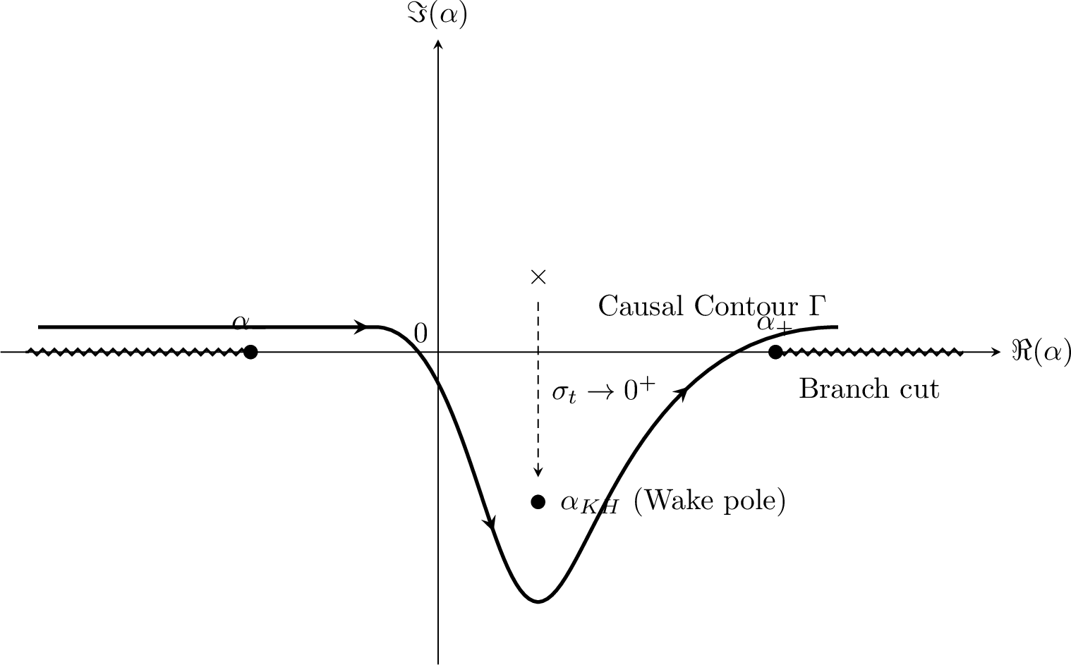
Theorem 16 (Flat-plate pole-residue formula). Assume Assumptions 1, 3, Hypotheses 4, 6 and \(C_-^{(KH)}\neq0\). Then, with the wake normalization 10 , \(\displaystyle A_{\mathrm{rec}}(\Omega,\mathcal{G}) = - \frac{ \langle \mathbf{F}_{\mathrm{inc}}(\Omega),\Psi^\ast(\Omega)\rangle_{\mathcal{H}_\sigma}}{ \langle \mathbf{F}_{KH}(\Omega),\Psi^\ast(\Omega)\rangle_{\mathcal{H}_\sigma}} = i\mathop{\mathrm{Res}}_{\alpha=\alpha_{KH}} \mathcal{M}(\alpha;\omega_{\rm phys},\mathcal{G})\). For a simple pole, \(\displaystyle A_{\mathrm{rec}}(\Omega,\mathcal{G}) = \frac{i\,\mathcal{N}(\alpha_{KH};\omega_{\rm phys},\mathcal{G})}{\partial_\alpha\mathcal{D}(\alpha_{KH};\omega_{\rm phys},\mathcal{G})}\).
Proof. By 9, bounded lower-deck matching selects the unique Kutta-normalized outer solution. By Corollary 2, the Kutta-normalized Wiener–Hopf solution is the same outer solution. The causal inverse transform 62 –64 gives the coefficient of the normalized \(\Phi_{KH}^{\rm out}\) as \(i\mathop{\mathrm{Res}}_{\alpha=\alpha_{KH}}\mathcal{M}\). The adjoint quotient is the same coefficient by 61 . The simple-pole expression follows from \(\displaystyle \mathcal{D}(\alpha)= \partial_\alpha\mathcal{D}(\alpha_{KH})(\alpha-\alpha_{KH}) +O((\alpha-\alpha_{KH})^2)\). ◻
The formula is invariant under the rescaling \[\Phi_{KH}^{\rm out}\mapsto c\Phi_{KH}^{\rm out},\qquad A\mapsto c^{-1}A,\] provided the same rescaling is used in \(\mathbf{F}_{KH}\), \(C_-^{(KH)}\), and \(\ell_{KH}\); the statement above fixes \(c\) by 10 . If \[\mathcal{D}(\alpha_{KH})=\mathcal{D}_\alpha(\alpha_{KH})=\cdots =\mathcal{D}_{\alpha}^{(m-1)}(\alpha_{KH})=0,\qquad \mathcal{D}_{\alpha}^{(m)}(\alpha_{KH})\neq0,\] then \(\displaystyle \mathcal{M}(\alpha) = \sum_{\ell=1}^{m} \frac{\mathcal{R}_\ell}{(\alpha-\alpha_{KH})^\ell} +\mathcal{M}_{\rm hol}(\alpha)\), and the downstream contribution is \(\displaystyle \eta_{KH}(x) = i\,e^{i\alpha_{KH}x} \sum_{\ell=1}^{m} \frac{(ix)^{\ell-1}}{(\ell-1)!}\mathcal{R}_\ell\). Thus the simple quotient \(i\mathcal{N}/\mathcal{D}_\alpha\) is valid only when \(\alpha_{KH}\) is simple. The geometry derivative of the simple-pole coefficient is \[\begin{align} \partial_\gamma A_{\mathrm{rec}} &= i\,\frac{\mathcal{N}_\gamma+\mathcal{N}_\alpha\partial_\gamma\alpha_{KH}}{\mathcal{D}_\alpha} - i\,\frac{\mathcal{N}(\mathcal{D}_{\alpha\gamma} +\mathcal{D}_{\alpha\alpha}\partial_\gamma\alpha_{KH})}{\mathcal{D}_\alpha^2},\\ \partial_\gamma\alpha_{KH} &= -\frac{\mathcal{D}_\gamma}{\mathcal{D}_\alpha}, \end{align}\] all quantities being evaluated at \((\alpha,\omega_{\rm phys},\mathcal{G})=(\alpha_{KH},\omega_{\rm phys},\mathcal{G})\). Thus, for the flat plate, \(\displaystyle A_{\mathrm{rec}} = i\mathop{\mathrm{Res}}_{\alpha=\alpha_{KH}}\mathcal{M}(\alpha;\omega_{\rm phys},\mathcal{G})\), and, together with 9, \[\label{eq:full-final-identity} \text{Fredholm lower-deck compatibility} \Longleftrightarrow C_-(A)=0 \Longleftrightarrow \text{wake-pole residue selection}.\tag{65}\] The Mellin analogue for finite-angle wedges with self-similar sheet data, including the wedge pole-residue formula (18), is given in Appendix 8.
6 Discussion and limitations↩︎
We summarize the conditional theory. Let \[\Phi_A^{\rm out}=\Phi_0^{\rm out}+A\Phi_{KH}^{\rm out},\qquad C_-(A)=C_-^{(0)}+A C_-^{(KH)},\qquad C_-^{(KH)}\neq0,\] and assume the simple-pole, edge-indicial, Fredholm (with augmented solvability), edge-concomitant, and Kutta-normalized transform hypotheses: \[\begin{gather} \mathcal{D}(\alpha_{KH};\omega_{\rm phys},\mathcal{G})=0,\qquad \mathcal{D}_\alpha(\alpha_{KH};\omega_{\rm phys},\mathcal{G})\neq0,\qquad \Im\alpha_{KH}<0,\\ \mathop{\mathrm{ind}}\mathcal{L}_{\mathrm{TD}}(\Omega)=0,\qquad \ker\mathcal{L}_{\mathrm{TD}}(\Omega)^\ast=\mathop{\mathrm{span}}\{\Psi^\ast(\Omega)\},\qquad \kappa(\Omega)=\mathscr{B}_{\mathrm{edge}}(r^{-1/2}\mathbf{V}_{-},\Psi^\ast(\Omega))\neq0,\\ \mathcal{M}(\alpha;\omega_{\rm phys},\mathcal{G}) = \frac{\mathcal{N}(\alpha;\omega_{\rm phys},\mathcal{G})}{\mathcal{D}(\alpha;\omega_{\rm phys},\mathcal{G})} \quadnear \alpha_{KH}. \end{gather}\] Then the selected amplitude is, with the wake normalization 10 , \[A_{\mathrm{rec}}(\Omega,\mathcal{G}) = -\frac{ \langle \mathbf{F}_{\mathrm{inc}}(\Omega),\Psi^\ast(\Omega)\rangle_{\mathcal{H}_\sigma}}{ \langle \mathbf{F}_{KH}(\Omega),\Psi^\ast(\Omega)\rangle_{\mathcal{H}_\sigma}} = -\frac{C_-^{(0)}}{C_-^{(KH)}} = i\mathop{\mathrm{Res}}_{\alpha=\alpha_{KH}} \mathcal{M}(\alpha;\omega_{\rm phys},\mathcal{G}).\] For a simple pole, \(\displaystyle A_{\mathrm{rec}}(\Omega,\mathcal{G}) = \frac{i\,\mathcal{N}(\alpha_{KH};\omega_{\rm phys},\mathcal{G})}{\mathcal{D}_\alpha(\alpha_{KH};\omega_{\rm phys},\mathcal{G})}\). Equivalently, \(C_-(A)=0\) iff \(\displaystyle \Pi_{\rm sing}F_{\rm match}(A)=0\) iff \(\displaystyle \mathbf{F}_{\mathrm{inc}}+A\mathbf{F}_{KH}\in\mathop{\mathrm{Ran}}\mathcal{L}_{\mathrm{TD}}(\Omega)\) iff \(\displaystyle \langle \mathbf{F}_{\mathrm{inc}}+A\mathbf{F}_{KH},\Psi^\ast\rangle_{\mathcal{H}_\sigma}=0\). Thus the unsteady Kutta condition is the vanishing of the singular edge trace, not an additional inviscid boundary condition: \[\operatorname{Tr}_{\mathrm{sing}}\nabla\phi_A^{\rm out} = C_-(A)r^{-1/2}\mathbf{V}_{-} =0 \quad\Longleftrightarrow\quad \mathscr{B}_{\mathrm{edge}}(C_-(A)r^{-1/2}\mathbf{V}_{-},\Psi^\ast)=0 .\] For the linear-shear model of 4 the inner hypotheses are theorems (Propositions 13 and 14), the adjoint state is the Airy-derivative field of 11, and the identities above hold unconditionally for all \(\Omega>0\) outside a discrete resonance set (Corollary 1). The distinguished frequency variable is \[\Omega = Re^{-1/4}\frac{\omega_{\rm phys}L}{U}, \qquad \Omega=O(1) \Longleftrightarrow \frac{\omega_{\rm phys}L}{U}=O(Re^{1/4}).\] Hence the leading receptivity law has the reduced form \(\displaystyle A_{\mathrm{rec}} = A_{\mathrm{rec}}\!\left( Re^{-1/4}\frac{\omega_{\rm phys}L}{U},\mathcal{G} \right)\). For a smooth one-parameter geometry \(\mathcal{G}=\mathcal{G}(\gamma)\), the simple-pole sensitivity is \[\begin{align} \partial_\gamma A_{\mathrm{rec}} &= i\,\frac{\mathcal{N}_\gamma+\mathcal{N}_\alpha\,\partial_\gamma\alpha_{KH}}{\mathcal{D}_\alpha} - i\,\frac{\mathcal{N}(\mathcal{D}_{\alpha\gamma} +\mathcal{D}_{\alpha\alpha}\partial_\gamma\alpha_{KH})}{\mathcal{D}_\alpha^2},\\ \partial_\gamma\alpha_{KH} &= -\frac{\mathcal{D}_\gamma}{\mathcal{D}_\alpha}, \end{align}\] with all functions evaluated at \((\alpha,\omega_{\rm phys},\mathcal{G})=(\alpha_{KH},\omega_{\rm phys},\mathcal{G})\). Thus \(\displaystyle \partial_\gamma A_{\mathrm{rec}} = \mathcal{S}_{\rm force} + \mathcal{S}_{\rm pole} + \mathcal{S}_{\rm dispersion}\), where \[\mathcal{S}_{\rm force}=\frac{i\,\mathcal{N}_\gamma}{\mathcal{D}_\alpha},\qquad \mathcal{S}_{\rm pole} = i\,\partial_\gamma\alpha_{KH} \left( \frac{\mathcal{N}_\alpha}{\mathcal{D}_\alpha} - \frac{\mathcal{N}\mathcal{D}_{\alpha\alpha}}{\mathcal{D}_\alpha^2} \right),\qquad \mathcal{S}_{\rm dispersion} = -\frac{i\,\mathcal{N}\mathcal{D}_{\alpha\gamma}}{\mathcal{D}_\alpha^2}.\] The Mellin analogue for finite-angle wedges with self-similar sheet data is given in Appendix 8.
Limitations and extensions↩︎
The full trailing-edge base flow introduces three analytic issues that are not settled here. (i) Fredholm realization: one must construct weighted spaces for the true unsteady lower-deck operator of [18], [19], [24], prove the index-zero Fredholm property 35 –36 , and establish the augmented solvability of Hypothesis 4(ii); the natural route is the limit-operator decomposition used in Proposition 13, with the explicit Airy symbols replaced by the frozen symbols of the numerically known base flow [60]. (ii) Edge nondegeneracy: one must prove \(\kappa(\Omega)\neq0\) for the corresponding adjoint state; Proposition 14 proves it in the model, where the adjoint is Airy-explicit. (iii) Spectral degenerations: multiple wake poles, pole–cut collisions with the acoustic branch points 8 , Briggs–Bers pinches (the absolute/convective transition, which invalidates the causal downstream pickup of 5.3 [42]–[44]), and the pole strings generated by non-self-similar wedge sheets [14] all require separate treatment; for a pole of order \(m\) the residue formula is replaced by the algebraically growing term \(\eta_{KH}(x)=i e^{i\alpha_{KH}x}\sum_{\ell=1}^{m} \tfrac{(ix)^{\ell-1}}{(\ell-1)!}\mathcal{R}_\ell\).
7 Formal adjoint and concomitant↩︎
Let \[\Pi=\mathbb{R}_X\times\mathbb{R}_+,\qquad \Gamma_p=(-\infty,0)\times\{0\},\qquad \Gamma_w=(0,\infty)\times\{0\}.\] The steady lower-deck state satisfies \[U_{0X}+V_{0Y}=0,\qquad V_0|_{\Gamma_w}=0 .\] For \(W=(u,v,p,a)^{\mathsf T}\), define \[R_0(W):=u_X+v_Y ,\] \[R_1(W):= -i\Omega u+U_0u_X+V_0u_Y+U_{0X}u+U_{0Y}v+p_X-u_{YY}.\] The primal homogeneous boundary and matching constraints are \[u=v=0\quad\text{on }\Gamma_p,\qquad v=0,\quad u_Y=0\quad\text{on }\Gamma_w,\] \[u(X,Y)-a(X)\to0\quad(Y\to\infty),\qquad p=\mathcal{K}[a].\] Here \(\mathcal{K}=H\partial_X\) such that \(\displaystyle \widehat{\mathcal{K}f}(\alpha)=|\alpha|\widehat f(\alpha)\). (For the two-sided wake of 3.2 the computation below is performed on each half \(\pm Y>0\) and the centerline terms of 19 are added; the symmetric component reproduces exactly the formulas of this appendix, and the antisymmetric component differs only in the wake-side boundary block.)
Bulk adjoint↩︎
Let \(\Psi=(u^\ast,q)^{\mathsf T}\). Pair \(\displaystyle \langle \mathcal{L}_{\mathrm{TD}}W,\Psi\rangle := \iint_{\Pi}\{u^\ast R_1(W)+qR_0(W)\}\,dX\,dY\) . Modulo boundary fluxes, \[\begin{align} \iint_\Pi u^\ast U_0u_X &\equiv -\iint_\Pi (U_0u_X^\ast+U_{0X}u^\ast)u,\\ \iint_\Pi u^\ast V_0u_Y &\equiv -\iint_\Pi (V_0u_Y^\ast+V_{0Y}u^\ast)u,\\ \iint_\Pi u^\ast p_X &\equiv -\int_{\mathbb{R}}p\,\bar U_X^\ast\,dX,\qquad \bar U^\ast(X):=\int_0^\infty u^\ast(X,Y)\,dY,\\ -\iint_\Pi u^\ast u_{YY} &\equiv -\iint_\Pi u_{YY}^\ast u,\qquad \iint_\Pi q u_X\equiv-\iint_\Pi q_Xu,\\ \iint_\Pi qv_Y&\equiv-\iint_\Pi q_Yv . \end{align}\] Therefore \[\begin{align} \langle \mathcal{L}_{\mathrm{TD}}W,\Psi\rangle &= \iint_\Pi u\, \Big( -i\Omega u^\ast-U_0u_X^\ast-U_{0X}u^\ast -V_0u_Y^\ast-V_{0Y}u^\ast +U_{0X}u^\ast-u_{YY}^\ast-q_X \Big)\,dX\,dY\\ &\quad+ \iint_\Pi v\,(U_{0Y}u^\ast-q_Y)\,dX\,dY - \int_{\mathbb{R}}p\,\bar U_X^\ast\,dX + \int_{\partial\Pi}J\cdot n\,ds . \end{align}\] Using \(V_{0Y}=-U_{0X}\), this becomes \[\langle \mathcal{L}_{\mathrm{TD}}W,\Psi\rangle = \iint_\Pi u\,\mathcal{L}_u^\ast\Psi\,dX\,dY + \iint_\Pi v\,\mathcal{L}_v^\ast\Psi\,dX\,dY - \int_{\mathbb{R}}p\,\bar U_X^\ast\,dX + \int_{\partial\Pi}J\cdot n\,ds ,\] where \[\mathcal{L}_u^\ast\Psi = -i\Omega u^\ast-U_0u_X^\ast-V_0u_Y^\ast +U_{0X}u^\ast-u_{YY}^\ast-q_X, \qquad \mathcal{L}_v^\ast\Psi = U_{0Y}u^\ast-q_Y .\] Hence the formal adjoint equations are \[-i\Omega u^\ast-U_0u_X^\ast-V_0u_Y^\ast +U_{0X}u^\ast-u_{YY}^\ast-q_X=0, \qquad q_Y=U_{0Y}u^\ast .\]
Concomitant↩︎
The boundary fluxes are \[J^X=qu+U_0u^\ast u+u^\ast p,\qquad J^Y=qv+V_0u^\ast u-(u^\ast u_Y-u_Y^\ast u).\] Equivalently, \[J = (J^X,J^Y),\qquad J^X=qu+U_0u^\ast u+u^\ast p,\quad J^Y=qv+V_0u^\ast u-u^\ast u_Y+u_Y^\ast u .\] The Lagrange identity is \[u^\ast R_1(W)+qR_0(W) - u\,\mathcal{L}_u^\ast\Psi - v\,\mathcal{L}_v^\ast\Psi = \partial_XJ^X+\partial_YJ^Y -p\,\bar U_X^\ast\delta_{Y=\infty},\] where the last term is understood after integration in \(Y\), equivalently as the line contribution \(-\int_{\mathbb{R}}p\,\bar U_X^\ast\,dX\).
Adjoint wall and wake conditions↩︎
On \(\Gamma_p\), the primal variations satisfy \(u=v=0\), while \(u_Y\) is free. Hence \(\displaystyle J^Y|_{\Gamma_p} = -u^\ast u_Y\), so vanishing of the boundary form for all admissible \(u_Y\) gives \(u^\ast=0\) on \(\Gamma_p\). On \(\Gamma_w\), the primal variations satisfy \(v=0\), \(u_Y=0\), and \(V_0=0\). Hence \(\displaystyle J^Y|_{\Gamma_w} = u_Y^\ast u\), so vanishing for arbitrary admissible \(u\) gives \(u_Y^\ast=0\) on \(\Gamma_w\). Thus \[u^\ast=0\;(X<0,Y=0),\qquad u_Y^\ast=0\;(X>0,Y=0),\] with decay conditions chosen so that the fluxes at \(X=\pm\infty\) and \(Y=\infty\) vanish in the weighted graph norm (with the weights 33 , adjoint states decay downstream faster than \(e^{-\vartheta X}\)).
Adjoint of the interaction and matching constraints↩︎
Introduce line multipliers \(b,\mu\) for \[p-\mathcal{K}[a]=0,\qquad a-u_\infty=0,\qquad u_\infty(X):=\lim_{Y\to\infty}u(X,Y).\] The augmented line pairing is \[\mathscr I_{\rm line} = -\int_{\mathbb{R}}p\,\bar U_X^\ast\,dX + \int_{\mathbb{R}}b(p-\mathcal{K}a)\,dX + \int_{\mathbb{R}}\mu(a-u_\infty)\,dX .\] The coefficient of \(p\) gives \[-\bar U_X^\ast+b=0 \quad\Longrightarrow\quad b=\bar U_X^\ast.\] The coefficient of \(a\) gives \(\displaystyle \mu-\mathcal{K}^\ast b=0\). Since \[H^\ast=-H,\qquad \partial_X^\ast=-\partial_X,\qquad H\partial_X=\partial_XH,\] we have \(\displaystyle \mathcal{K}^\ast=(H\partial_X)^\ast = \partial_X^\ast H^\ast = (-\partial_X)(-H) = H\partial_X = \mathcal{K}\). Equivalently, in Fourier variables, \[\widehat{\mathcal{K}f}(\alpha)=|\alpha|\widehat f(\alpha) \quad\Longrightarrow\quad \mathcal{K}^\ast=\mathcal{K}\ge0 .\] Thus \(\displaystyle \mu=\mathcal{K}b=\mathcal{K}[\bar U_X^\ast]=H[\bar U_{XX}^\ast]\). The coefficient of \(u_\infty\) is \(-\mu\), the adjoint far-field traction associated with the displacement matching.
Compact operator form↩︎
With \[\Psi^\ast=(u^\ast,q,b,\mu)^{\mathsf T}, \qquad \bar U^\ast(X)=\int_0^\infty u^\ast(X,Y)\,dY,\] the formal adjoint of the linearized lower-deck operator is \(\displaystyle \mathcal{L}_{\mathrm{TD}}(\Omega)^\ast\Psi^\ast=0\), meaning \[\begin{cases} -i\Omega u^\ast-U_0u_X^\ast-V_0u_Y^\ast +U_{0X}u^\ast-u_{YY}^\ast-q_X=0,\\[1mm] q_Y=U_{0Y}u^\ast,\\[1mm] b=\bar U_X^\ast,\\[1mm] \mu=\mathcal{K}[\bar U_X^\ast], \end{cases}\] with \[u^\ast=0\quad\text{on }\Gamma_p,\qquad u_Y^\ast=0\quad\text{on }\Gamma_w.\] For admissible \(W\) and \(\Psi^\ast\), \[\label{eq:app-Green} \langle \mathcal{L}_{\mathrm{TD}}(\Omega)W,\Psi^\ast\rangle_{\mathcal{H}_\sigma} - \langle W,\mathcal{L}_{\mathrm{TD}}(\Omega)^\ast\Psi^\ast\rangle_{\mathcal{H}_\sigma} = \int_{\partial\Pi}J(W,\Psi^\ast)\cdot n\,ds + \int_{\mathbb{R}} \{b(p-\mathcal{K}a)+\mu(a-u_\infty)\}\,dX .\tag{66}\] If \(W\in\mathcal{D}(\mathcal{L}_{\mathrm{TD}})\) and \(\Psi^\ast\in\mathcal{D}(\mathcal{L}_{\mathrm{TD}}^\ast)\), all boundary and line terms vanish except possible finite edge contributions.
Finite edge concomitant↩︎
Let \(B_\rho^+=\Pi\cap\{X^2+Y^2<\rho^2\}\). For a singular edge datum \[G=C\,r^{-1/2}\mathbf{V}_{-}(\theta)\in\mathcal{E}_{\mathrm{edge}},\qquad \mathcal{E}_{\mathrm{edge}}=\mathop{\mathrm{span}}\{r^{-1/2}\mathbf{V}_{-}\},\] with lower-deck line traces \((g_\infty^\sharp,g_K^\sharp)\) given by 27 –28 , define \[\mathscr{B}_{\mathrm{edge}}(G,\Psi^\ast) := \mathop{\mathrm{f.p.}}\lim_{\rho\downarrow0} \int_{\partial B_\rho^+} J(G,\Psi^\ast)\cdot n\,ds + \mathop{\mathrm{f.p.}}\int_{\mathbb{R}} \big(g_K^\sharp\,b+g_\infty^\sharp\,\mu\big)\,dX .\] The second (trace-pairing) term is the contribution of the pressure–displacement and matching constraints, i.e., the line pairing of 66 evaluated on the singular datum; it is the form used in the model computation of 4. The finite parts exist because the bulk profile is locally square integrable in two dimensions, the line traces pair against the adjoint line states with local exponents summing above \(-1\), and the residual divergences are removed by the finite part. Linearity yields \(\displaystyle \mathscr{B}_{\mathrm{edge}}(C\,r^{-1/2}\mathbf{V}_{-},\Psi^\ast) = C\,\mathscr{B}_{\mathrm{edge}}(r^{-1/2}\mathbf{V}_{-},\Psi^\ast)\). Thus the edge nondegeneracy condition used in the main text is exactly \(\displaystyle \kappa(\Omega) := \mathscr{B}_{\mathrm{edge}}(r^{-1/2}\mathbf{V}_{-},\Psi^\ast(\Omega)) \neq0\). For the outer family, \(\displaystyle \mathscr{B}_{\mathrm{edge}}(C_-(A)r^{-1/2}\mathbf{V}_{-},\Psi^\ast(\Omega)) = C_-(A)\kappa(\Omega)\).
Resulting compatibility formula↩︎
For decomposed matching data \[F_{\rm match}(A) = C_-(A)\mathbf{F}_{\mathrm{sing}}+\mathbf{F}_{\mathrm{inc}}+A\mathbf{F}_{KH}, \qquad \mathbf{F}_{\mathrm{sing}}\in\mathcal{E}_{\mathrm{edge}},\quad \mathbf{F}_{\mathrm{inc}}+A\mathbf{F}_{KH}\in\mathcal{H}_\sigma,\] the Green identity 66 , applied under the augmented solvability of Hypothesis 4(ii), gives the generalized solvability condition \(\displaystyle C_-(A)\kappa(\Omega) + \langle \mathbf{F}_{\mathrm{inc}}(\Omega)+A\mathbf{F}_{KH}(\Omega), \Psi^\ast(\Omega)\rangle_{\mathcal{H}_\sigma} = 0\). Read as an identity in \(A\) (Proposition 7), this gives \(\langle\mathbf{F}_{\mathrm{inc}}+A\mathbf{F}_{KH},\Psi^\ast\rangle=-\kappa(\Omega)C_-(A)\), hence \(\chi=-\kappa\). If the lower-deck solution is required to belong to the bounded graph domain \(\mathcal{X}_\sigma\), then the singular component is excluded, \(\displaystyle \Pi_{\rm sing}F_{\rm match}(A)=C_-(A)\mathbf{F}_{\mathrm{sing}}=0\), and therefore \(\displaystyle C_-(A)=0\) iff \(\displaystyle \operatorname{Tr}_{\mathrm{sing}}\nabla\phi_A^{\rm out}=0\) iff \(\displaystyle \langle \mathbf{F}_{\mathrm{inc}}+A\mathbf{F}_{KH},\Psi^\ast\rangle_{\mathcal{H}_\sigma}=0\). Consequently, \(\displaystyle A = -\frac{ \langle \mathbf{F}_{\mathrm{inc}}(\Omega),\Psi^\ast(\Omega)\rangle_{\mathcal{H}_\sigma}}{ \langle \mathbf{F}_{KH}(\Omega),\Psi^\ast(\Omega)\rangle_{\mathcal{H}_\sigma}} = -\frac{C_-^{(0)}}{C_-^{(KH)}}\).
8 Mellin analogue for finite-angle wedges↩︎
Let the edge be a wedge \[\Pi_\Theta=\{(r,\theta):r>0,\;-\Theta_-<\theta<\Theta_+\}, \qquad \Theta=\Theta_-+\Theta_+ .\] For local wedge fields use the Mellin transform \[\mathfrak M[f](s) = \int_0^\infty r^{s-1}f(r)\,dr,\qquad f(r)=\frac{1}{2\pi i}\int_{\Re s=\sigma} r^{-s}\mathfrak M[f](s)\,ds .\] A structural caveat is required which has no flat-plate counterpart. The Mellin transform diagonalizes dilations, not translations; a wake mode that is asymptotically a plane wave \(e^{i\alpha x}\) far from the edge is not Mellin-homogeneous, and for general wedge sheets the instability emerges from infinite pole strings \(\{s_{KH}-n\}_{n\geq0}\) generated by the functional-difference structure rather than from a single pole—this is precisely the careful treatment that the instability-wave amplitude requires in [14]. A single-residue statement is therefore meaningful only on the dilation-invariant class:
Assumption 4 (Self-similar sheet class). The base sheet data in \(\mathcal{G}\) are self-similar (sheet strength a pure power of \(r\)), so that the homogeneous wake modes of the wedge problem are Mellin-homogeneous, \(\eta_{KH}\propto r^{-s_{KH}}\), the wake functional \(\ell_{KH}\) is the coefficient of \(r^{-s_{KH}}\), and the Kutta-normalized response 68 is meromorphic near a simple wake pole \(s_{KH}\).
The principal separated solutions are \[\phi(r,\theta)=r^\lambda\Phi_\lambda(\theta),\qquad \Phi_\lambda''+\lambda^2\Phi_\lambda=0,\] or, in Mellin notation, \(\lambda=-s\). The wedge walls and sheet conditions produce a finite-dimensional functional-difference system [14], [56] \[\label{eq:Mellin-difference} \mathbb{A}(s;\Omega,\mathcal{G})\mathbf{U}(s) + \mathbb{B}(s;\Omega,\mathcal{G})\mathbf{U}(s-1) = \mathbf{F}(s;\Omega,\mathcal{G}),\tag{67}\] where \(\mathbf{U}(s)\) collects Mellin transforms of the angular trace amplitudes and sheet displacement. Its homogeneous determinant is \(\displaystyle \mathcal{D}_{\rm wedge}(s;\Omega,\mathcal{G}) := \det\mathbb{T}(s;\Omega,\mathcal{G})\), after reduction of the difference system to a period-one transfer matrix \(\mathbb{T}\). The Kutta-normalized wedge response is assumed meromorphic: \[\label{eq:wedge-M} \mathcal{M}_{\rm wedge}(s;\Omega,\mathcal{G}) = \frac{\mathcal{N}_{\rm wedge}(s;\Omega,\mathcal{G})}{\mathcal{D}_{\rm wedge}(s;\Omega,\mathcal{G})} .\tag{68}\] The wedge faces carry the rigid Neumann conditions \(\partial_\theta\phi=0\) at \(\theta=-\Theta_-,\Theta_+\), so the angular pencil \(\Phi_\lambda''+\lambda^2\Phi_\lambda=0\) with \(\Phi_\lambda'(-\Theta_-)=\Phi_\lambda'(\Theta_+)=0\) has the Neumann spectrum \[\lambda_n(\Theta)=\frac{n\pi}{\Theta},\qquad n=0,1,2,\ldots,\qquad \Theta=\Theta_-+\Theta_+,\] with eigenfunctions \(\Phi_{\lambda_n}(\theta)=\cos\!\big(\tfrac{n\pi}{\Theta}(\theta+\Theta_-)\big)\). The first nonconstant root is the loading (pressure-jump) mode \[\lambda_-(\Theta)=\frac{\pi}{\Theta},\qquad \Psi_-^{(\Theta)}(\theta) = \cos\!\Big(\frac{\pi}{\Theta}(\theta+\Theta_-)\Big),\] which at the cusped/flat-plate value \(\Theta=2\pi\) reduces to \(\lambda_-=\tfrac12\) and \(\Psi_-^{(\Theta)}=-\sin\tfrac{\theta}{2}\), recovering Assumption 2. The associated velocity singularity is \(r^{\lambda_-(\Theta)-1}\), genuinely singular precisely when \(\lambda_-(\Theta)<1\), i.e. \(\Theta>\pi\); the admissible trailing-edge range is therefore \(\Theta\in(\pi,2\pi]\), the singularity (and with it the Kutta selection) disappearing as \(\Theta\downarrow\pi\). The wedge singular edge-trace space is \(\displaystyle \mathcal{E}_{\mathrm{edge}}^{(\Theta)} = \mathop{\mathrm{span}}\{r^{\lambda_-(\Theta)-1}\mathbf{V}_{-}^{(\Theta)}\}\), replacing \(\mathcal{E}_{\mathrm{edge}}=\mathop{\mathrm{span}}\{r^{-1/2}\mathbf{V}_{-}\}\) in the lower-deck hypotheses. The edge singularity \(r^{\lambda_-(\Theta)}\Psi_-^{(\Theta)}(\theta)\) corresponds to a Mellin pole at \(\displaystyle s=-\lambda_-(\Theta)=-\frac{\pi}{\Theta}\) under the convention \(\mathfrak M[r^\lambda]\sim(s+\lambda)^{-1}\). Thus the wedge Kutta normalization is \[\mathop{\mathrm{Res}}_{s=-\pi/\Theta}\mathcal{M}_{\rm wedge}(s;\Omega,\mathcal{G})=0, \qquad C_-(A)=0 ,\] which collapses to \(\mathop{\mathrm{Res}}_{s=-1/2}=0\) only in the cusped limit \(\Theta=2\pi\).
Remark 17 (Separation of edge and wake poles). For \(\mathcal{M}_{\rm wedge}\) to be well defined near the wake pole \(s_{KH}\), the edge pole and the wake pole must remain distinct, \(s_{KH}\neq-\pi/\Theta\): the normalization kills the edge pole and the residue reads off the wake pole. For thin trailing edges \(\Theta\to2\pi\) this is automatic; as \(\Theta\to\pi^+\) the edge pole \(-\pi/\Theta\to-1\) migrates and may in principle collide with a wake pole.
Let \(s_{KH}\) be a simple unstable wake pole: \[\label{eq:wedge-KH-pole} \mathcal{D}_{\rm wedge}(s_{KH};\Omega,\mathcal{G})=0,\qquad \partial_s\mathcal{D}_{\rm wedge}(s_{KH};\Omega,\mathcal{G})\neq0 .\tag{69}\] Then the inverse Mellin deformation gives \[\eta(r) = \frac{1}{2\pi i}\int_{\Re s=\sigma} r^{-s}\mathcal{M}_{\rm wedge}(s;\Omega,\mathcal{G})\,ds = \sum_{s_j\in\mathcal{P}} \mathop{\mathrm{Res}}_{s=s_j}\big(r^{-s}\mathcal{M}_{\rm wedge}(s)\big) +\eta_{\rm rem}(r),\] the orientation factor being unity here (\(\tfrac1{2\pi i}\cdot2\pi i=1\), in contrast with the Fourier factor \(i\) of 63 ), and the unstable wedge-mode coefficient is \(\displaystyle A_{\rm pole}^{\rm wedge}(\Omega,\mathcal{G}) = \mathop{\mathrm{Res}}_{s=s_{KH}}\mathcal{M}_{\rm wedge}(s;\Omega,\mathcal{G})\). For a simple pole, \(\displaystyle A_{\rm pole}^{\rm wedge}(\Omega,\mathcal{G}) = \frac{\mathcal{N}_{\rm wedge}(s_{KH};\Omega,\mathcal{G})}{\partial_s\mathcal{D}_{\rm wedge}(s_{KH};\Omega,\mathcal{G})}\).
Theorem 18 (Mellin pole-residue formula). Assume Assumption 4, the wedge Mellin representation 68 , the simple pole condition 69 , and the lower-deck hypotheses Hypotheses 4 and 6. Then \[\label{eq:wedge-main} A_{\mathrm{rec}}^{\rm wedge}(\Omega,\mathcal{G}) = - \frac{ \langle \mathbf{F}_{\mathrm{inc}}^{\rm wedge}(\Omega),\Psi^\ast_{\rm wedge}(\Omega) \rangle_{\mathcal{H}_\sigma}}{ \langle \mathbf{F}_{KH}^{\rm wedge}(\Omega),\Psi^\ast_{\rm wedge}(\Omega) \rangle_{\mathcal{H}_\sigma}} = \mathop{\mathrm{Res}}_{s=s_{KH}} \mathcal{M}_{\rm wedge}(s;\Omega,\mathcal{G}).\tag{70}\] If \(s_{KH}\) is simple, then \(\displaystyle A_{\mathrm{rec}}^{\rm wedge}(\Omega,\mathcal{G}) = \frac{\mathcal{N}_{\rm wedge}(s_{KH};\Omega,\mathcal{G})}{\partial_s\mathcal{D}_{\rm wedge}(s_{KH};\Omega,\mathcal{G})}\).
Proof. The Mellin transform diagonalizes the radial homogeneity and, under Assumption 4, converts the wedge trace equations into 67 with a Mellin-homogeneous wake mode. Kutta normalization removes the \(s=-\pi/\Theta\) edge pole, hence fixes the same one-dimensional kernel as \(C_-(A)=0\). The conditional lower-deck theorem identifies this Kutta-normalized wedge solution with the Fredholm-selected one. The inverse Mellin formula then gives the coefficient of the unstable wedge mode as the residue at \(s=s_{KH}\), which yields 70 ; the simple-pole formula follows by the Laurent expansion of \(\mathcal{D}_{\rm wedge}\). ◻
Together with 9, the wedge analogue of 65 holds verbatim, with \(i\mathop{\mathrm{Res}}_{\alpha=\alpha_{KH}}\mathcal{M}\) replaced by \(\mathop{\mathrm{Res}}_{s=s_{KH}}\mathcal{M}_{\rm wedge}\) and the edge space \(\mathcal{E}_{\mathrm{edge}}\) by \(\mathcal{E}_{\mathrm{edge}}^{(\Theta)}\).