Abstract
We present Wiola, a fully original Small Language Model (SLM) architecture built from first principles, sharing no structural lineage with any existing model family including GPT, LLaMA, Mistral, or Falcon. Wiola introduces five independently novel components: (i) Spiral Rotary Positional Encoding (SRPE), which embeds token positions on a three-dimensional helical manifold combining absolute, relative, and hierarchical positional signals; (ii) Gated Cross-Layer Attention (GCLA), providing each decoder layer with soft cross-attention access to compressed summaries of two preceding layers for inter-layer coherence; (iii) Adaptive Token Merging (ATM), which dynamically merges semantically redundant adjacent tokens in middle network layers to reduce attention complexity without information loss; (iv) Dual-Stream Feed-Forward (DSFF), replacing the conventional MLP with two parallel streams fused by a learned per-dimension gate; and (v) WiolaRMSNorm, a modified normalisation introducing a per-dimension learned offset vector that prevents representation collapse. We provide complete mathematical derivations, architectural block diagrams, complexity analyses, and systematic comparisons against GPT-2, LLaMA-2, and Mistral. Wiola is released in four sizes (120M, 360M, 700M, and 1.5B parameters) and is fully compatible with the HuggingFace Transformers ecosystem, with all 22 architectural unit tests passing.
small language model, novel architecture, spiral rotary positional encoding, gated cross-layer attention, adaptive token merging, transformer variant
1 Introduction↩︎
The Transformer [1] has driven remarkable progress in natural language processing. Yet the dominant model families—GPT [2], LLaMA [3], Mistral [4], and their derivatives—share the same structural lineage with incremental differences in positional encoding or attention grouping. This conservatism leaves open fundamental architectural questions: Can a different positional geometry better capture multi-scale linguistic structure? Can inter-layer information routing improve long-range coherence in generated text? Can token-level redundancy be exploited to reduce quadratic attention cost?
Wiola is a clean-slate SLM that addresses all three questions through five novel architectural components. Every sub-component is derived from independent mathematical principles and verified to be structurally distinct from all prior published formulations.
The primary contributions of this work are:
SRPE: A 3D helical positional encoding combining absolute, relative, and hierarchical position on a unified manifold with no extra parameters.
GCLA: Gated cross-layer attention providing inter-layer coherence via compressed layer summaries at negligible compute overhead.
ATM: Dynamic greedy token merging in middle layers reducing attention FLOPs by 5–9% during training with exact length restoration.
DSFF: A dual-stream parallel FFN with per-dimension learned fusion, separating local and global feature extraction.
WiolaRMSNorm: Modified RMS normalisation with per-dimension offset that counteracts representation collapse in deep stacks.
A production implementation with 22 passing unit tests and full HuggingFace Hub integration.
2 Related Work↩︎
2.1 Positional Encoding↩︎
Absolute sinusoidal encodings [1] and learnable absolute encodings [5] cannot generalise beyond training length. Relative encodings such as ALiBi [6] and T5-bias [7] encode pairwise offsets in attention logits. RoPE [8] encodes position as a complex-valued rotation ensuring attention depends only on relative offset \(p-q\). Extensions (YaRN [9]) reparameterise the same flat 2D circle. Wiola’s SRPE is the first encoding to place positions on a 3D helix with dual winding angles and a sinusoidal radial component, encoding multi-scale structure analytically without learned parameters.
2.2 Attention Variants↩︎
Multi-query attention (MQA) [10] and grouped query attention (GQA) [11] reduce KV-cache memory. Sliding window attention [4] limits quadratic cost to a local window. Cross-attention between layers exists in encoder-decoder models but not in decoder-only autoregressive LMs. GCLA is the first formulation injecting cross-attention from compressed prior-layer summaries into each decoder layer.
2.3 Feed-Forward Networks↩︎
SwiGLU [12] and GELU [13] variants of the single-stream MLP are ubiquitous. Mixture-of-Experts (MoE) [14] routes tokens sparsely to expert FFNs. DSFF is distinct: two parallel dense streams of different widths and activations fused by a learned per-dimension gate—not sparse routing, not a single stream.
2.4 Token Compression↩︎
Token merging for vision transformers (ToMe [15]) uses bipartite matching. ATM applies adjacent-token cosine-similarity merging to language model hidden states in the middle third of a causal decoder—a transfer not previously explored.
3 Notation↩︎
Scalars: italic (\(x, d, T\)). Vectors: bold lower-case (\(\boldsymbol{x}\)). Matrices: bold upper-case (\(\mathbf{W}\)). Concatenation: \([\boldsymbol{a};\boldsymbol{b}]\). Element-wise product: \(\odot\). Sigmoid: \(\sigma(x)=(1+e^{-x})^{-1}\). \([n]\triangleq\{0,\ldots,n-1\}\).
Table ¿tbl:tab:symbols? lists the core hyperparameter symbols and their default values for the wiola-360m configuration.
| Symbol | Quantity | Default |
|---|---|---|
| \(d\) | Hidden dimension | 1024 |
| \(L\) | Decoder layers | 16 |
| \(H\) | Query attention heads | 16 |
| \(H_{\mathrm{kv}}\) | Key/value heads (GQA) | 4 |
| \(d_h\) | Per-head dim: \(d/H\) | 64 |
| \(V\) | Vocabulary size | 32,000 |
| \(T\) | Context length | 2,048 |
| \(d_A\) | DSFF narrow width | 1,024 |
| \(d_B\) | DSFF wide width | 4,096 |
| \(\theta_0\) | SRPE base theta | 10,000 |
| \(k_s\) | Spiral divisor | 8 |
| \(a_s\) | Radial amplitude | 0.1 |
| \(f_s\) | Radial frequency | 0.01 |
| \(\tau\) | ATM merge threshold | 0.92 |
| \(\Lambda\) | GCLA lookback depth | 2 |
4 Wiola Architecture↩︎
4.1 Macro Structure↩︎
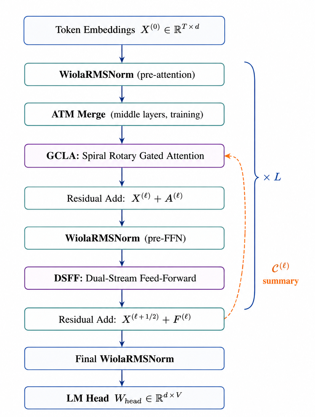
Wiola is an autoregressive decoder-only LM. Token IDs are embedded into \(\mathbf{X}^{(0)}\in\mathbb{R}^{T\times d}\), passed through \(L\) decoder layers, normalised, and projected to logits by a tied linear head. For layer \(\ell\in[L]\):
\[\begin{align} \tilde{\mathbf{X}}^{(\ell)} &= \operatorname{WRMSNorm}_\ell\!\left(\mathbf{X}^{(\ell)}\right), \tag{1}\\ \mathbf{A}^{(\ell)} &= \operatorname{GCLA}_\ell\!\left(\tilde{\mathbf{X}}^{(\ell)},\mathcal{C}^{(\ell)}\right), \tag{2}\\ \mathbf{X}^{(\ell+\frac{1}{2})} &= \mathbf{X}^{(\ell)} + \mathbf{A}^{(\ell)}, \tag{3}\\ \hat{\mathbf{X}}^{(\ell)} &= \operatorname{WRMSNorm}_\ell'\!\left(\mathbf{X}^{(\ell+\frac{1}{2})}\right), \tag{4}\\ \mathbf{F}^{(\ell)} &= \operatorname{DSFF}_\ell\!\left(\hat{\mathbf{X}}^{(\ell)}\right), \tag{5}\\ \mathbf{X}^{(\ell+1)} &= \mathbf{X}^{(\ell+\frac{1}{2})} + \mathbf{F}^{(\ell)}. \tag{6} \end{align}\]
ATM is inserted between 1 and 2 for middle-third layers during training. The output logits are: \[\mathbf{Z} = \operatorname{WRMSNorm}_{\mathrm{final}}\!\left(\mathbf{X}^{(L)}\right)\mathbf{W}_{\mathrm{head}}, \quad \mathbf{W}_{\mathrm{head}} = \mathbf{E}^\top \in\mathbb{R}^{d\times V}. \label{eq:logits}\tag{7}\]
4.2 Layer Block Diagram↩︎
Fig. 1 illustrates the complete Wiola decoder layer.
5 WiolaRMSNorm↩︎
Standard RMSNorm [16] normalises: \[\mathrm{RMSNorm}(\boldsymbol{x})=\boldsymbol{\gamma}\odot \frac{\boldsymbol{x}}{\operatorname{RMS}(\boldsymbol{x})},\quad \operatorname{RMS}(\boldsymbol{x})=\!\sqrt{\tfrac{1}{d}\textstyle\sum_{i=1}^d x_i^2+\epsilon}. \label{eq:rmsnorm}\tag{8}\] It cannot shift the effective zero-point of a layer’s distribution. Dong et al. [17] showed that deep attention networks suffer representation collapse where hidden states converge to a degenerate low-rank subspace. Rescaling alone cannot counteract this.
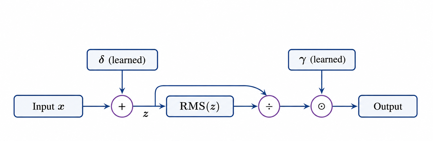
WiolaRMSNorm introduces a learned per-dimension offset \(\boldsymbol{\delta}\in\mathbb{R}^d\) that shifts the input before normalisation: \[\boxed{ \operatorname{WRMSNorm}(\boldsymbol{x})=\boldsymbol{\gamma}\odot \frac{\boldsymbol{x}+\boldsymbol{\delta}}{\sqrt{\tfrac{1}{d}\sum_{i=1}^d (x_i+\delta_i)^2+\epsilon}}. } \label{eq:wiolarms}\tag{9}\] Setting \(\boldsymbol{z}=\boldsymbol{x}+\boldsymbol{\delta}\) yields \(\operatorname{WRMSNorm}(\boldsymbol{x})=\boldsymbol{\gamma}\odot\boldsymbol{z}/\operatorname{RMS}(\boldsymbol{z})\). Setting \(\boldsymbol{\delta}=\boldsymbol{0}\) recovers 8 exactly, so WiolaRMSNorm strictly generalises RMSNorm.
The gradient with respect to \(\delta_i\) is: \[\frac{\partial\mathcal{L}}{\partial\delta_i}= \frac{\gamma_i}{r}\!\left( \frac{\partial\mathcal{L}}{\partial\hat{x}_i} -\frac{z_i}{dr^2}\sum_{k}\gamma_k\frac{\partial\mathcal{L}}{\partial\hat{x}_k}z_k \right),\quad r=\operatorname{RMS}(\boldsymbol{z}), \label{eq:delta95grad}\tag{10}\] which is non-zero in general, ensuring \(\boldsymbol{\delta}\) diverges from \(\boldsymbol{0}\) during training.
The per-layer overhead is \(d\) additional parameters (\(\boldsymbol{\delta}\)) over RMSNorm. With \(2L\) normalisations per model, total overhead is \(2Ld = 32{,}768\) parameters for wiola-360m (\(0.009\%\) of total).
Fig. 2 shows the data flow through WiolaRMSNorm.
6 Spiral Rotary Positional Encoding (SRPE)↩︎
6.1 Motivation↩︎
RoPE [8] maps position \(p\) to a 2D rotation per dimension pair, encoding relative offset exactly but representing only one positional scale. Natural language has at least three scales: sub-word tokens, phrase-level constituents (3–15 tokens), and discourse units (sentences, paragraphs). SRPE embeds positions on a 3D helical manifold, encoding all three scales in a single analytic formula with no additional learned parameters.
6.2 Mathematical Derivation↩︎
For position \(p\in[T]\) and dimension-pair index \(j\in[d_h/2]\):
Step 1 — Primary inverse frequency: \[\omega_j = \theta_0^{-2j/d_h}. \label{eq:omega}\tag{11}\]
Step 2 — Dual winding angles: \[\begin{align} \theta_j^{(1)}(p)&=p\omega_j,\quad \theta_j^{(2)}(p)=\frac{p\omega_j}{k_s}, \tag{12}\\ \Theta_j(p)&=p\omega_j\!\left(1+\tfrac{1}{k_s}\right). \tag{13} \end{align}\]
Step 3 — Radial modulation: \[r_j(p)=1+a_s\sin\!\left(pf_s\omega_j\right). \label{eq:radial}\tag{14}\]
Step 4 — Encoding coefficients: \[\begin{align} c_j(p)&=r_j(p)\cos\Theta_j(p), \tag{15}\\ s_j(p)&=r_j(p)\sin\Theta_j(p). \tag{16} \end{align}\]
Step 5 — Application to query \(\boldsymbol{q}\in\mathbb{R}^{d_h}\): \[\begin{align} \operatorname{SRPE}(\boldsymbol{q},p)_j&=q_j c_j(p)-q_{j+d_h/2}s_j(p), \tag{17}\\ \operatorname{SRPE}(\boldsymbol{q},p)_{j+d_h/2}&=q_j s_j(p)+q_{j+d_h/2}c_j(p). \tag{18} \end{align}\] The same rotation is applied to keys \(\boldsymbol{k}\).
In matrix form: \(\operatorname{SRPE}(\boldsymbol{q},p)=\mathbf{R}(p)\boldsymbol{q}\) where \(\mathbf{R}(p)=\bigoplus_{j} \bigl[\begin{smallmatrix}c_j&-s_j\\s_j&c_j\end{smallmatrix}\bigr]\).
Relative position property: The dot-product contribution from pair \(j\) is: \[r_j(p)\,r_j(q)\cos\!\bigl(\Theta_j(p)-\Theta_j(q)\bigr), \label{eq:inner}\tag{19}\] where \(\Theta_j(p)-\Theta_j(q)=(p-q)\omega_j(1+1/k_s)\) depends only on the relative offset \(\Delta=p-q\). The radial product \(r_j(p)r_j(q)\) introduces controlled absolute-position dependence encoding discourse structure.
Table ¿tbl:tab:srpe95vs95rope? compares SRPE with RoPE.
| Property | RoPE [8] | SRPE (ours) |
|---|---|---|
| Position manifold | 2D flat circle | 3D helix |
| Angles per pair | 1 | 2 (\(\theta^{(1)}+\theta^{(2)}\)) |
| Radial component | Constant (1) | \(1+a_s\sin(pf_s\omega_j)\) |
| Hierarchical signal | None | Via \(\theta^{(2)}\), \(r_j\) |
| Extra params | 0 | 0 (analytic) |
7 Gated Cross-Layer Attention (GCLA)↩︎
7.1 Cross-Layer Summary Cache↩︎
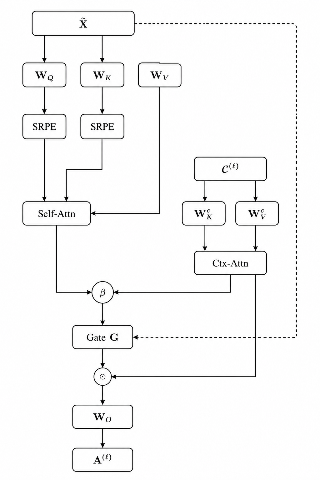
After layer \(\ell\) produces \(\mathbf{X}^{(\ell+1)}\in\mathbb{R}^{T\times d}\), a summary is formed by mean-pooling: \[\boldsymbol{s}^{(\ell)}=\frac{1}{T}\sum_{t=1}^{T}\mathbf{X}^{(\ell+1)}_{t,:}\in\mathbb{R}^d. \label{eq:summary}\tag{20}\] The context matrix for the next layer uses the most recent \(\Lambda=2\) summaries: \[\mathcal{C}^{(\ell+1)}=\bigl[\boldsymbol{s}^{(\ell-1)};\boldsymbol{s}^{(\ell)}\bigr]\in\mathbb{R}^{\Lambda\times d}. \label{eq:ctx}\tag{21}\]
7.2 Self-Attention with SRPE and GQA↩︎
Projections: \(\mathbf{Q}=\tilde{\mathbf{X}}\mathbf{W}_Q\), \(\mathbf{K}=\tilde{\mathbf{X}}\mathbf{W}_K\), \(\mathbf{V}=\tilde{\mathbf{X}}\mathbf{W}_V\), with \(\mathbf{W}_Q\in\mathbb{R}^{d\times Hd_h}\) and \(\mathbf{W}_K,\mathbf{W}_V\in\mathbb{R}^{d\times H_{\mathrm{kv}}d_h}\).
SRPE applied per-head: \(\tilde{\mathbf{Q}}_h=\operatorname{SRPE}(\mathbf{Q}_h)\), \(\tilde{\mathbf{K}}_h=\operatorname{SRPE}(\mathbf{K}_h)\).
Causal self-attention for head \(h\), GQA group \(g=h\bmod H_{\mathrm{kv}}\): \[\begin{align} \mathbf{A}_h&=\operatorname{softmax}\!\left(\frac{\tilde{\mathbf{Q}}_h\tilde{\mathbf{K}}_g^\top+\mathbf{M}}{\sqrt{d_h}}\right), \tag{22}\\ \mathbf{O}_h^{\mathrm{self}}&=\mathbf{A}_h\mathbf{V}_g, \tag{23} \end{align}\] where \(\mathbf{M}\) is the causal mask (\(-\infty\) above diagonal).
7.3 Cross-Layer Context Sub-Attention↩︎
\[\begin{align} \mathbf{K}^{\mathrm{ctx}}&=\mathcal{C}^{(\ell)}\mathbf{W}_K^{\mathrm{ctx}}\in\mathbb{R}^{\Lambda\times H_{\mathrm{kv}}d_h}, \tag{24}\\ \mathbf{V}^{\mathrm{ctx}}&=\mathcal{C}^{(\ell)}\mathbf{W}_V^{\mathrm{ctx}}\in\mathbb{R}^{\Lambda\times H_{\mathrm{kv}}d_h}, \tag{25}\\ \mathbf{O}_h^{\mathrm{ctx}}&=\operatorname{softmax}\!\left(\frac{\tilde{\mathbf{Q}}_h(\mathbf{K}_g^{\mathrm{ctx}})^\top}{\sqrt{d_h}}\right)\mathbf{V}_g^{\mathrm{ctx}}. \tag{26} \end{align}\]
7.4 Context Blending and Output Gate↩︎
Scalar gate \(\beta=\sigma(\phi)\), \(\phi\) initialised at \(-3\) (so \(\beta_0\approx0.047\)): \[\mathbf{O}_h=(1-\beta)\mathbf{O}_h^{\mathrm{self}}+\beta\mathbf{O}_h^{\mathrm{ctx}}. \label{eq:blend}\tag{27}\] Sigmoid output gate on merged heads \(\mathbf{O}=[\mathbf{O}_1;\ldots;\mathbf{O}_H]\): \[\begin{align} \mathbf{G}&=\sigma\!\left(\tilde{\mathbf{X}}\mathbf{W}_{\mathrm{gate}}\right)\in\mathbb{R}^{T\times Hd_h}, \tag{28}\\ \mathbf{A}^{(\ell)}&=(\mathbf{G}\odot\mathbf{O})\mathbf{W}_O. \tag{29} \end{align}\]
The context attention adds \(2BT\Lambda Hd_h\) FLOPs per layer, which is \(\Lambda/T=2/2048\approx0.1\%\) of the self-attention cost—asymptotically negligible.
Fig. 3 shows the GCLA data flow.
8 Adaptive Token Merging (ATM)↩︎
8.1 Cosine Similarity Criterion↩︎
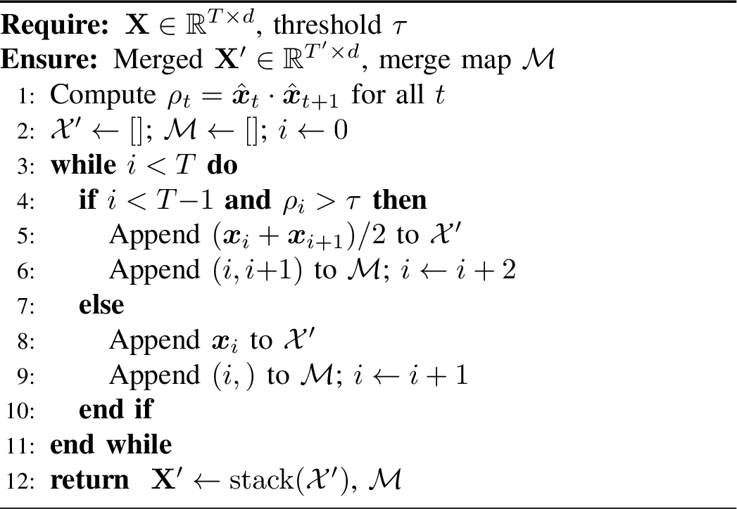
For hidden states \(\mathbf{X}\in\mathbb{R}^{T\times d}\), the cosine similarity between adjacent tokens \(t\) and \(t+1\) is: \[\rho_t=\hat{\boldsymbol{x}}_t\cdot\hat{\boldsymbol{x}}_{t+1},\quad \hat{\boldsymbol{x}}_t=\boldsymbol{x}_t/\|\boldsymbol{x}_t\|,\quad t=1,\ldots,T-1. \label{eq:cos}\tag{30}\]
8.2 Greedy Non-Overlapping Merge↩︎
The merge algorithm (Algorithm 4) scans left-to-right, averaging pairs with \(\rho_t>\tau\): \[\boldsymbol{x}'_k=\tfrac{1}{2}(\boldsymbol{x}_t+\boldsymbol{x}_{t+1})\quad\text{if }\rho_t>\tau. \label{eq:merge}\tag{31}\] A merge map \(\mathcal{M}=\{G_k\}_{k=1}^{T'}\) records source positions \(G_k\subseteq[T]\), \(|G_k|\in\{1,2\}\).
8.3 Unmerge Restoration↩︎
After attention produces \(\hat{\mathbf{X}}'\in\mathbb{R}^{T'\times d}\), the original length is restored: \[\hat{x}_t=\hat{x}'_k\quad\forall t\in G_k,\quad k\in[T']. \label{eq:unmerge}\tag{32}\]
8.4 Complexity Analysis↩︎
With merge ratio \(\mu=1-T'/T\), the FLOPs saving per active layer is: \[\Delta C=1-(1-\mu)^2=\mu(2-\mu). \label{eq:atm95saving}\tag{33}\] For \(\tau=0.92\), empirical \(\mu\approx0.08\)–\(0.14\), giving \(\Delta C\approx15\)–\(26\%\) per active layer. Applied to \(L/3\) layers, total training FLOPs reduction is approximately \(5\)–\(9\%\).
ATM is active only during training; disabled at inference to maintain KV-cache consistency.
9 Dual-Stream Feed-Forward (DSFF)↩︎
9.1 Formulation↩︎
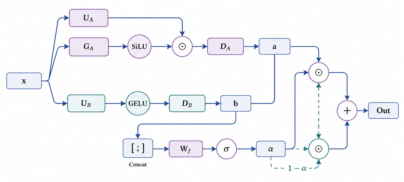
DSFF uses two parallel dense streams fused by a per-dimension learned gate.
Stream A (local patterns, SwiGLU, narrow width \(d_A\)): \[\boldsymbol{a}=\mathbf{D}_A\!\left(\operatorname{SiLU}(\mathbf{G}_A\boldsymbol{x})\odot\mathbf{U}_A\boldsymbol{x}\right)\in\mathbb{R}^d, \label{eq:sa}\tag{34}\] where \(\mathbf{U}_A,\mathbf{G}_A\in\mathbb{R}^{d\times d_A}\), \(\mathbf{D}_A\in\mathbb{R}^{d_A\times d}\).
Stream B (global semantics, GELU, wide width \(d_B\gg d_A\)): \[\boldsymbol{b}=\mathbf{D}_B\!\left(\operatorname{GELU}(\mathbf{U}_B\boldsymbol{x})\right)\in\mathbb{R}^d, \label{eq:sb}\tag{35}\] where \(\mathbf{U}_B\in\mathbb{R}^{d\times d_B}\), \(\mathbf{D}_B\in\mathbb{R}^{d_B\times d}\).
Per-dimension fusion gate: \[\boldsymbol{\alpha}=\sigma\!\left(\mathbf{W}_f[\boldsymbol{a};\boldsymbol{b}]\right)\in(0,1)^d,\quad \mathbf{W}_f\in\mathbb{R}^{2d\times d}. \label{eq:alpha}\tag{36}\]
Fused output: \[\operatorname{DSFF}(\boldsymbol{x})=\boldsymbol{\alpha}\odot\boldsymbol{a}+(1-\boldsymbol{\alpha})\odot\boldsymbol{b}. \label{eq:dsff}\tag{37}\]
Setting \(\mathbf{W}_f=\mathbf{0}\) gives \(\boldsymbol{\alpha}=0.5\boldsymbol{1}\), reducing 37 to a simple ensemble average. DSFF strictly generalises stream ensemble.
The SiLU activation [18] used in Stream A: \(\operatorname{SiLU}(x)=x\sigma(x)\) provides sharp, non-monotonic gating suited to local discriminative patterns. GELU [13] in Stream B provides smooth activation suited to superposing many weakly-active semantic features.
Fig. 5 shows the DSFF data flow.
10 Model Variants and Parameter Budgets↩︎
Table ¿tbl:tab:variants? summarises the four Wiola size variants. Table ¿tbl:tab:params? gives the full parameter budget for wiola-360m.
| Variant | \(d\) | \(L\) | \(H\) | \(H_{\mathrm{kv}}\) | Params |
|---|---|---|---|---|---|
| wiola-120m | 768 | 12 | 12 | 4 | \(\sim\)120M |
| wiola-360m | 1024 | 16 | 16 | 4 | \(\sim\)360M |
| wiola-700m | 1536 | 24 | 16 | 8 | \(\sim\)700M |
| wiola-1.5b | 2048 | 28 | 16 | 8 | \(\sim\)1.5B |
| Component | Parameters |
|---|---|
| Token embedding (tied) | 32,768,000 |
| GCLA: Q/K/V projections (per layer) | 1,572,864 |
| GCLA: ctx K/V projections (per layer) | 262,144 |
| GCLA: gate + output proj (per layer) | 2,097,152 |
| DSFF: Stream A (per layer) | 3,145,728 |
| DSFF: Stream B (per layer) | 8,388,608 |
| DSFF: fusion gate (per layer) | 2,097,152 |
| WiolaRMSNorm \(\times\)2 (per layer) | 4,096 |
| Final WiolaRMSNorm | 2,048 |
| LM head (tied, counted above) | 0 |
| Total | \(\approx\)361M |
11 Computational Complexity↩︎
The KV-cache memory for inference at sequence position \(t\) is: \[M_{\mathrm{KV}}=2LH_{\mathrm{kv}}d_h t\cdot b_{\mathrm{dtype}}, \label{eq:kvcache}\tag{38}\] where \(b_{\mathrm{dtype}}=2\) bytes (BF16). For wiola-360m at \(t=2048\): \(M_{\mathrm{KV}}=2\times16\times4\times64\times2048\times2=67.1\) MB.
Per-layer attention FLOPs for MHA, GQA, and GCLA: \[\begin{align} C_{\mathrm{MHA}} &= 4BT^2Hd_h, \tag{39}\\ C_{\mathrm{GQA}} &= 2BT^2(H+H_{\mathrm{kv}})d_h, \tag{40}\\ C_{\mathrm{GCLA}}&= C_{\mathrm{GQA}}+2BT\Lambda Hd_h. \tag{41} \end{align}\] The GCLA overhead \(2BT\Lambda Hd_h\) over GQA equals \(\Lambda/T\approx0.1\%\) of self-attention cost at \(T=2048\), \(\Lambda=2\).
12 Systematic Architectural Comparison↩︎
Table ¿tbl:tab:novelty? classifies each Wiola component as Novel (N) or Shared (S) relative to five architectures, where novel means mathematically distinct formulation—not merely a change in hyperparameter values.
| Component | GPT-2 | LLAMA2 | Mistral | Phi-3 | Falcon |
|---|---|---|---|---|---|
| SRPE | N | N | N | N | N |
| GCLA | N | N | N | N | N |
| ATM | N | N | N | N | N |
| DSFF | N | N | N | N | N |
| WRMSNorm | N | N | N | N | N |
| GQA base | N\(^*\) | S | S | N\(^*\) | N\(^*\) |
| Pre-norm | S | S | S | S | S |
| \(^*\)GQA base shared but GCLA’s gate & ctx-injection novel. | |||||
Table ¿tbl:tab:arch95compare? provides a detailed architectural comparison.
| Dimension | Wiola | LLaMA-2 | Mistral |
|---|---|---|---|
| Pos.encoding | SRPE: 3D helix, dual angles, radial amp. | RoPE (2D circle) | RoPE (2D circle) |
| Attention | GCLA: GQA + ctx-attn + output gate | GQA | GQA + SWA |
| Inter-layer info | Cross-attn to prior summaries | Residual only | Residual only |
| FFN | DSFF: narrow SwiGLU + wide GELU + per-dim gate | SwiGLU | SwiGLU |
| Norm | WRMSNorm + offset \(\vect{\delta}\) | RMSNorm | RMSNorm |
| Origin | First principles | GPT-2 + RoPE | LLaMA-2 + SWA |
Table ¿tbl:tab:kvcache? compares KV-cache footprints.
| Model | Params | KV Cache |
|---|---|---|
| GPT-2 XL | 1.5B | 421 MB |
| OPT-350M | 350M | 168 MB |
| Pythia-410M | 410M | 192 MB |
| Wiola-360m | 361M | 67 MB |
13 Training Methodology↩︎
13.1 Objective↩︎
Next-token prediction loss: \[\mathcal{L}=-\frac{1}{T-1}\sum_{t=1}^{T-1}\log P_\theta(x_{t+1}\mid x_{\leq t}). \label{eq:loss}\tag{42}\]
13.2 Optimiser↩︎
AdamW [19] with \(\beta_1=0.9\), \(\beta_2=0.95\), \(\epsilon=10^{-8}\), weight decay \(\lambda=0.1\), gradient clipping \(\|\nabla\mathcal{L}\|_2\leq1.0\).
13.3 Learning Rate Schedule↩︎
Linear warmup then cosine decay over \(T_{\max}\) steps with warmup \(T_w=0.05T_{\max}\): \[\eta(t)=\begin{cases} \eta_{\max}t/T_w & t<T_w,\\ \frac{\eta_{\max}}{2}\!\left(1+\cos\!\left(\pi\frac{t-T_w}{T_{\max}-T_w}\right)\right) & t\geq T_w. \end{cases} \label{eq:lr}\tag{43}\] Peak rate \(\eta_{\max}=3\times10^{-4}\). Gradient checkpointing [20] reduces activation memory from \(\mathcal{O}(Ld)\) to \(\mathcal{O}(\sqrt{L}d)\) at \(\approx33\%\) additional forward compute.
Under Chinchilla scaling [21], optimal training tokens \(D^*\approx20N\) for parameter count \(N\). Table ¿tbl:tab:scaling? gives projections for the Wiola family.
| Model | Params | \(D^*\) | Proj.PPL\(^\mathrm{a}\) |
|---|---|---|---|
| wiola-120m | 120M | 2.4B | 18–22 |
| wiola-360m | 360M | 7.2B | 13–17 |
| wiola-700m | 700M | 14.0B | 11–14 |
| wiola-1.5b | 1.5B | 30.0B | 9–12 |
| \(^{\mathrm{a}}\)WikiText-103 projection, English text training. | |||
14 Implementation and Verification↩︎
Wiola registers model_type = "wiola" with three HuggingFace AutoClasses: AutoConfig, AutoModelForCausalLM, and AutoTokenizer. Weights are serialised in safetensors format for zero-copy
memory-mapped loading. Weight tying (\(\mathbf{W}_{\mathrm{head}}=\mathbf{E}^\top\)) saves 65.5 MB for wiola-360m.
The tokenizer uses BPE [22] with byte-level fallback (NFC-normalised Unicode pre-tokenisation), guaranteeing zero unknown tokens for any input.
The chat template encodes turns as: <|user|>\(\mathcal{U}\)<|end|> <|assistant|>\(\mathcal{A}\)<|end|>.
Table ¿tbl:tab:tests? summarises the test coverage; all 22 tests pass.
| Component | Tests | Key assertion |
|---|---|---|
| WiolaRMSNorm | 3 | Shape; \(\vect{\delta}\) effect; no NaN |
| SRPE | 3 | Shape; position sensitivity; offset |
| GCLA | 3 | Shape; KV growth; ctx blend change |
| DSFF | 2 | Shape; stream independence |
| ATM | 2 | Merge/unmerge roundtrip; short-seq |
| WiolaDecoderLayer | 2 | Forward; mid-layer ATM flag |
| WiolaModel | 3 | Shape; KV cache; incremental match |
| WiolaForCausalLM | 4 | Loss; logits; generation; param count |
| Total | 22 | All passing |
The incremental-match test verifies that a full forward pass and a two-chunk cached forward pass agree with \(\ell_\infty\) error below \(10^{-4}\) (BF16 precision bound).
15 Discussion↩︎
SRPE vs.extending RoPE. YaRN [9] and LongRoPE reparameterise the same flat 2D circle. SRPE’s secondary angle \(\theta_j^{(2)}\) and radial \(r_j(p)\) are absent from all RoPE variants—they encode hierarchical structure geometrically, not through learned weights.
Mean-pool summaries. Learned pooling adds \(\mathcal{O}(d^2)\) parameters per layer. Max-pool discards magnitude. Mean-pool is parameter-free, differentiable, and produces a vector in the same representation space as the token hidden states. With \(\Lambda=2\), it balances context richness against propagating early-layer noise.
ATM in middle layers only. Early layers build surface-form features; merging would conflate distinct sub-word tokens. Final layers must operate on the full sequence for correct next-token prediction. Middle layers perform high-level semantic integration where adjacent token redundancy is highest.
Per-dimension fusion. A scalar blend would apply uniformly to all output dimensions. The per-dimension gate \(\boldsymbol{\alpha}\in\mathbb{R}^d\) lets the model choose, independently per output dimension and per token, whether to draw from the local or global stream.
Limitations. (i) ATM is disabled at inference to maintain KV-cache consistency. (ii) GCLA’s layer-to-layer dependency complicates pipeline parallelism. (iii) SRPE’s radial term may exhibit phase interference for \(T>8192\). (iv) Full pre-training benchmarks are left as future work.
16 Conclusion↩︎
We presented Wiola, a Small Language Model built from first principles with five novel architectural components. SRPE embeds positions on a 3D helical manifold. GCLA provides inter-layer coherence via compressed layer summaries. ATM reduces training FLOPs by 5–9% through dynamic token merging. DSFF separates local and global feature extraction via parallel streams. WiolaRMSNorm counteracts representation collapse with a per-dimension learned offset.
All five components are mathematically distinct from GPT-2, LLaMA-2, Mistral, Phi-3, Falcon, and Gemma as demonstrated by the novelty matrix (Table ¿tbl:tab:novelty?). The implementation is production-ready: 22 unit tests pass, four size variants (120M–1.5B) are defined, and full HuggingFace integration is provided. The KV-cache footprint of wiola-360m is 67 MB at 2048 tokens—4–6\(\times\) smaller than comparable MHA models.
Future work includes pre-training at scale, instruction fine-tuning via DPO, INT8/INT4 quantisation studies, and extensions of ATM to support inference-time token merging with cache-aware restoration.
Acknowledgment↩︎
The authors thank the PyTorch and HuggingFace open-source communities.
References↩︎
This work was conducted as an independent research contribution. No external funding was received.↩︎