From Approximation to Emergence
A Theory of Deep Learning
July 01, 2026
Figure 1:  .
.
Preface↩︎
This monograph develops a structured account of several central theoretical questions in modern deep learning. Its starting point is the classical triad of approximation, optimization, and generalization, but its scope also includes phenomena that have become prominent in the era of overparameterized networks, foundation models, generative modeling, in-context learning, preference optimization, mechanistic interpretability, and emergent behavior. The aim is not to present a collection of instructional units, nor to function as a textbook organized around exercises. The aim is to synthesize scattered mathematical results into a coherent research narrative, to identify the assumptions under which different explanations are valid, and to clarify where present theory remains incomplete.
The manuscript treats deep learning theory as a family of partially overlapping explanatory programs. Approximation theory asks which target functions can be represented efficiently. Optimization theory asks when and why nonconvex training procedures reach useful solutions. Generalization theory asks why high-capacity models can perform well beyond the training sample. Robustness, distribution shift, generative modeling, scaling laws, interpretability, and alignment introduce additional questions that cannot be reduced to the classical triad alone. A recurring theme of the book is that each theoretical route reveals a genuine mechanism while also imposing a distinctive set of modeling assumptions.
The contribution of the book is therefore primarily synthetic and analytical: it reorganizes a broad literature around common objects, compares assumptions and conclusions across theories, and gives proof-oriented presentations of key results where the mathematical structure is most informative. Claims of original discovery are intentionally avoided unless they are explicitly supported by cited work or by material supplied by the author. The guiding principle is that attribution, assumptions, and proof status should remain visible: established theorems are cited, proof sketches are presented as sketches, and synthetic interpretations are separated from claims of new mathematical results.
The intended readers are researchers, graduate students, and mathematically trained practitioners who need a rigorous map of deep learning theory rather than an instructional manual. Readers are expected to be familiar with probability, linear algebra, optimization, and basic machine learning. The exposition keeps examples when they illuminate mechanisms or boundary cases, but removes the exercise-driven structure of the earlier instructional draft. The resulting book is meant to support scholarly use, proposal review, and publication as an academic monograph.
1 Orientation and Approximation Foundations↩︎
1.1 Introduction: Problems, Literature, and Contributions↩︎
Deep learning theory studies a class of learning systems whose empirical success exceeds the explanatory reach of any single classical framework. The field inherits foundational questions from statistical learning theory, approximation theory, convex optimization, and high-dimensional probability, but modern architectures introduce additional mechanisms: extreme overparameterization, data-dependent representation learning, implicit bias of training dynamics, scale-dependent behavior, distributional robustness, generative sampling, preference optimization, and internal feature structure. This monograph treats these topics as connected parts of one theoretical program rather than as isolated subfields.
1.1.1 The Object of Study↩︎
A supervised learning problem begins with a distribution over pairs \((x,y)\), a loss function, and a hypothesis class. Classical theory asks how large a sample must be in order for empirical risk minimization to approximate the best population-risk predictor in the class [1], [2]. Deep learning changes the emphasis. The hypothesis class is not merely large; it is parameterized by layered nonlinear maps whose geometry depends on architecture, initialization, optimization, data, and scale. The central object is therefore not only a function class, but a coupled system consisting of representation, training dynamics, and statistical selection.
The book organizes this system around four questions.
Organizing Questions
Expressive capacity. Which functions can deep architectures approximate efficiently, and when does depth reduce complexity relative to shallow representations [3]–[7]?
Optimization and selection. Why can gradient-based methods find useful solutions in nonconvex, overparameterized systems, and what implicit preference is imposed by the algorithm [8]–[12]?
Generalization and stability. How can high-capacity models avoid the failures predicted by naive complexity measures, and which bounds remain informative in modern regimes [13]–[16]?
Modern mechanisms. What additional theoretical tools are needed for robustness, generative models, transformers, scaling laws, interpretability, preference optimization, and emergent generalization [17]–[25]?
1.1.2 From Separate Results to a Coherent Theory↩︎
The literature on deep learning theory is broad because different mathematical models isolate different mechanisms. Approximation theory describes what can be represented before training is considered. Kernel and neural tangent kernel analyses describe training in regimes where features change slowly [8], [26], [27]. Mean-field and implicit regularization viewpoints emphasize how parameterization and dynamics bias the selected predictor. Stability and PAC-Bayes approaches connect algorithms to generalization, while distributional and computational lower bounds show where such explanations must fail or become conditional.
A useful monograph should not hide these differences. It should make the assumptions visible. For example, a theorem in the lazy-training regime may explain convergence at large width but may not explain feature learning. A uniform convergence bound may be valid but numerically loose in interpolating models. A robustness guarantee may require a threat model that is not implied by natural distribution shift. A scaling law may summarize empirical behavior without giving a complete causal mechanism. The chapters that follow therefore track three elements for each theory: the mathematical object being controlled, the assumptions under which the control is valid, and the phenomena left outside the model.
1.1.3 Conventions for Mathematical Status↩︎
Because the book combines classical theorems, modern proof sketches, empirical laws, and mechanism-level research programs, it uses explicit status markers. A statement labeled as a theorem, lemma, proposition, or corollary without an “informal” qualifier is intended to have mathematically specified hypotheses and either a proof in the text or a standard proof in the cited literature. A paragraph labeled “proof idea” or “proof sketch” records the mechanism of an argument but may omit technical regularity conditions, concentration constants, or limiting arguments that are not central to the chapter’s purpose.
Statements labeled “informal” should be read as precise research summaries rather than as new standalone theorems. They identify the mathematical object, the typical regime, and the qualitative conclusion, while leaving the exact technical formulation to the cited source. Similarly, formulas described as “schematic” are included to organize mechanisms or scaling relations; they are not asserted as universal equalities outside the stated model. This convention is important in deep learning theory, where the same empirical phenomenon may admit several incompatible idealizations. The aim is to keep the boundary visible between proven theorem, standard proof sketch, empirical law, and open research program.
1.1.4 Scope of the Monograph↩︎
Chapters on approximation and Barron theory establish the representational starting point. The discussion then moves to optimization, neural tangent kernels, adaptive methods, and implicit regularization. The middle part of the book treats generalization bounds, stability, double descent, distributional assumptions, and lower bounds. Later chapters extend the same analytical style to robustness, generative modeling, transformers, in-context learning, diffusion and flow matching, scaling laws, interpretability, grokking, preference optimization, out-of-distribution generalization, and emergence. The final chapter compares the theories and identifies open problems.
The manuscript intentionally avoids two extremes. It is not a catalogue of all known results in the field, and it is not a simplified instructional sequence. Instead, it selects results that reveal mechanisms and places them in a common framework. The selection reflects the existing draft and its available bibliography. Additional author-specific results should be incorporated only when they can be verified by publications, preprints, or complete proofs.
1.1.5 Scholarly Contribution and Limits↩︎
Relative to a standard textbook, the value of this manuscript lies in the systematic comparison of theoretical routes. It highlights how approximation, optimization, generalization, robustness, and modern foundation-model theory use different mathematical abstractions for the same empirical systems. It also records the limits of each abstraction: fixed-feature theories do not by themselves explain representation learning; classical capacity measures do not fully explain interpolation; empirical scaling relations do not replace mechanistic understanding; and emergent behavior requires care in separating true phase-like transitions from metric artifacts.
This cautious positioning is important for academic publication. The book can claim to offer a unified exposition, a comparative framework, and proof-oriented synthesis of a large literature. It should not claim unsupported original breakthroughs. The distinction between established results, the author’s organization of those results, and the author’s own new analysis is maintained through citations, attribution, and explicit statements of scope. If later versions add author-specific research contributions, they should be inserted as separate, verifiable statements tied to publications, preprints, or complete proofs, rather than blended into the exposition as unsupported novelty claims. This convention protects both the mathematical credibility of the book and the reader’s ability to distinguish theorem, interpretation, and research program.
1.1.6 Why Start with Approximation?↩︎
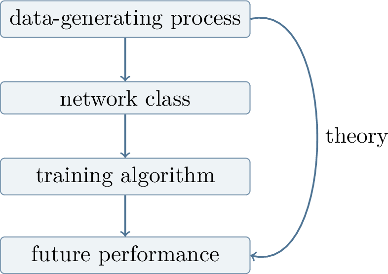
Deep learning theory begins with a deceptively simple question: what functions can neural networks express? The question is not merely about syntax or architecture. A trained network is useful only if three different events occur simultaneously. First, the chosen model class must contain, or at least closely approximate, a predictor with small population risk. Second, the training algorithm must be able to find parameters whose empirical objective is competitive. Third, the function selected from the finite sample must continue to perform well on unseen data. Approximation theory isolates the first of these requirements. It asks what the model class can represent before we discuss whether the representation is found by gradient descent or whether it generalizes from finitely many examples.
This separation of questions is a useful discipline. Without approximation results, there may be no good predictor to find. Without optimization theory, the existence of a good predictor may be computationally irrelevant. Without generalization theory, fitting the training sample may say little about future performance. The first chapter therefore studies approximation as the foundation on which the later optimization and generalization chapters build.
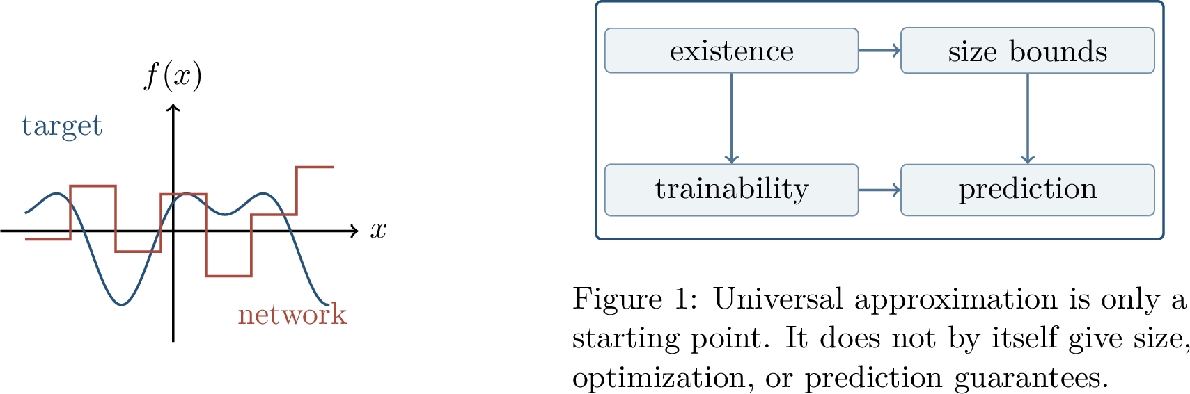
Two kinds of approximation results will be important. Universal approximation theorems, beginning with classical results such as those of Cybenko and Hornik [3], [28], give qualitative density statements: under broad assumptions, neural-network classes can approximate every continuous function on a compact set. Barron’s theorem [4] gives a more quantitative statement for a structured spectral class: a shallow network with \(k\) hidden units can achieve squared \(L^2\) error of order \(1/k\), with a constant that is not obtained by placing a grid in the ambient space. The contrast between these two messages is the central theme of the chapter. Universality tells us that approximation is possible; quantitative approximation asks whether it is efficient.
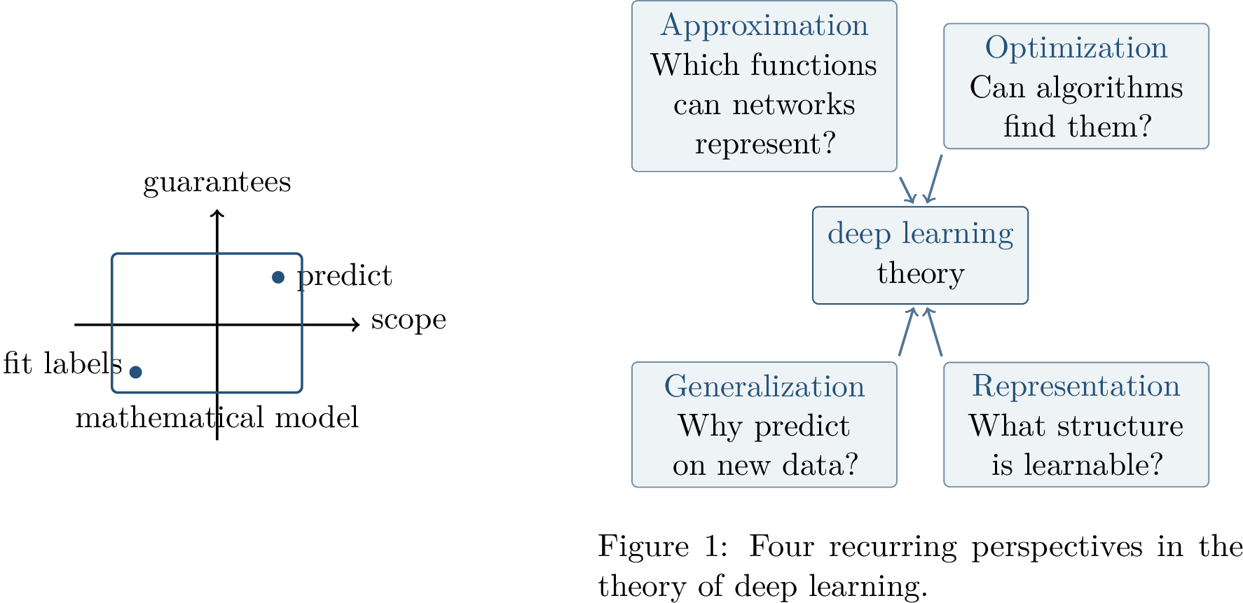
The monograph will repeatedly return to four lenses: approximation, optimization, generalization, and representation. Approximation asks which functions can be represented, and at what size. Optimization asks whether an algorithm can locate a good representative of the class. Generalization asks why a model chosen from observed data predicts well on new data. Representation asks what structure in the data, architecture, or training dynamics makes natural problems easier than arbitrary functions. The present chapter focuses on the first lens, but the other three must remain visible: an approximation theorem is a statement about the existence of functions, not a complete explanation of learning.
At the level of expressivity, the core question is the following.
Core Question What kinds of functions can we express with neural networks, and how many hidden units are needed for a useful approximation?
This question has both a qualitative and a quantitative form. The qualitative form asks whether the approximation error can be made arbitrarily small if the network is allowed to grow. The quantitative form asks how many parameters, layers, or hidden units are needed to reach a prescribed tolerance. In applications the second question is often the decisive one: a theorem requiring exponentially many units may be mathematically correct and practically uninformative at the same time.
1.1.7 The Learning Setup↩︎
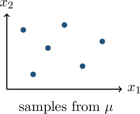
We now introduce the statistical notation used throughout the chapter. Let \(\mu\) be an unknown distribution on \(\R^d\times\mathcal{Y}\). A training sample is \[S=\{(x_i,y_i)\}_{i=1}^n,\qquad (x_i,y_i)\sim\mu,\] typically assumed independent and identically distributed. The vector \(x_i\in\R^d\) contains the observed features, and \(y_i\in\mathcal{Y}\) is the label or response. A predictor is a function \(f:\R^d\to\mathcal{Y}\), or more generally a scoring function whose output is converted into a prediction.
The assumption that the data are sampled from a common distribution is not a claim that real data are literally generated by a simple mechanism. It is a mathematical idealization that lets us distinguish the observed sample from the population on which we hope to perform well. The distribution \(\mu\) is not known to the learner. It enters the theory as the object with respect to which future performance is measured.
Definition 1.1 (Population and Empirical Risk). Given a loss \(\ell(\widehat y,y)\), the population risk and empirical risk are \[\mathcal{R}(f)=\E_{(x,y)\sim\mu}\bigl[\ell(f(x),y)\bigr], \qquad \widehat{\mathcal{R}}_S(f)=\frac{1}{n}\sum_{i=1}^n \ell(f(x_i),y_i).\]
The population risk \(\mathcal{R}(f)\) is the ideal quantity. It averages the loss over a fresh draw from the data-generating distribution. The empirical risk \(\widehat{\mathcal{R}}_S(f)\) is the computable quantity. It averages the same loss over the training sample. Learning algorithms usually minimize, or approximately minimize, empirical objectives; theory asks when this produces a function with small population risk.
Common losses include squared loss \[\ell(\widehat y,y)=\frac{1}{2}(y-\widehat y)^2\] for regression, and logistic loss \[\ell(\widehat y,y)=\log(1+\exp(-y\widehat y)), \qquad y\in\{\pm1\},\] for margin-based binary classification. The loss turns a learning task into an objective, but it rarely captures every property we ultimately care about. A network with small logistic loss may still be poorly calibrated, nonrobust, or unfair; these issues belong to later parts of the theory.
A Low-Dimensional Example For one-dimensional regression, \(x\in[0,1]\) and \(y=g(x)+\xi\), where \(\E[\xi\mid x]=0\). Under squared loss, the best population predictor is the conditional mean \(g(x)=\E[y\mid x]\). If we choose a network class \(\mathcal{F}\), the approximation question is whether some \(f\in\mathcal{F}\) is uniformly or \(L^2(\mu)\)-close to \(g\). The statistical question is different: from finitely many noisy samples, can an algorithm identify a member of \(\mathcal{F}\) whose population risk is nearly as good?
The approximation part of learning is visible in the usual decomposition. If \(\widehat f\) is the output of a training algorithm, \(\mathcal{F}\) is the chosen model class, and \(f^\star\) denotes an ideal population predictor, then formally \[\begin{align} \mathcal{R}(\widehat f)-\mathcal{R}(f^\star) &= \underbrace{\mathcal{R}(\widehat f)-\inf_{f\in\mathcal{F}}\mathcal{R}(f)} _{\text{optimization and statistical output}}\\ &\quad+ \underbrace{\inf_{f\in\mathcal{F}}\mathcal{R}(f)-\mathcal{R}(f^\star)} _{\text{approximation}}. \end{align}\] In a more refined analysis, the first term is further split into an optimization error and a sample-to-population generalization error. This chapter studies the second term: how expressive \(\mathcal{F}\) is relative to the target.
The decomposition is only formal unless the objects are specified carefully. For example, \(f^\star\) might be the Bayes predictor in a statistical model, the regression function \(x\mapsto\E[y\mid x]\), or a fixed target function in an approximation problem. Likewise, \(\inf_{f\in\mathcal{F}}\mathcal{R}(f)\) may fail to be attained if the parameterization is not compact. These technical distinctions are important in a full statistical theory, but the guiding interpretation is simple: approximation error measures the mismatch between the target and the chosen hypothesis class.
Definition 1.2 (Realizable and Probabilistic Concept Models). In the realizable case, there is a known hypothesis class \(\mathcal{H}\) and a target \(f^\star\in\mathcal{H}\) such that \(y=f^\star(x)\). A softer noisy-label model assumes that \[\E[y\mid x]=f^\star(x),\] so the label is not a deterministic function of the feature vector, but the conditional mean has structure.
The reference monograph emphasize simple examples of realizable classes. A halfspace classifier has the form \[f^\star(x)=\operatorname{sgn}(\left\langle a^\star,x \right\rangle+b^\star).\] Kernel methods give a richer version: choose a feature map \(\phi:\R^d\to\R^m\), or into a reproducing kernel Hilbert space, and use a linear rule after mapping the data into that feature space. This idea helps explain why nonlinear decision boundaries can arise from linear prediction in a larger representation.
The realizable assumption is strong. It says that the world already contains a perfect member of the hypothesized class. In modern deep learning this is best viewed as a clean mathematical starting point, not as a literal modeling claim. More commonly, the class \(\mathcal{F}\) is misspecified: no member is exactly correct, but some members may still approximate the relevant target well enough for the task. This is precisely the regime in which quantitative approximation results become informative.
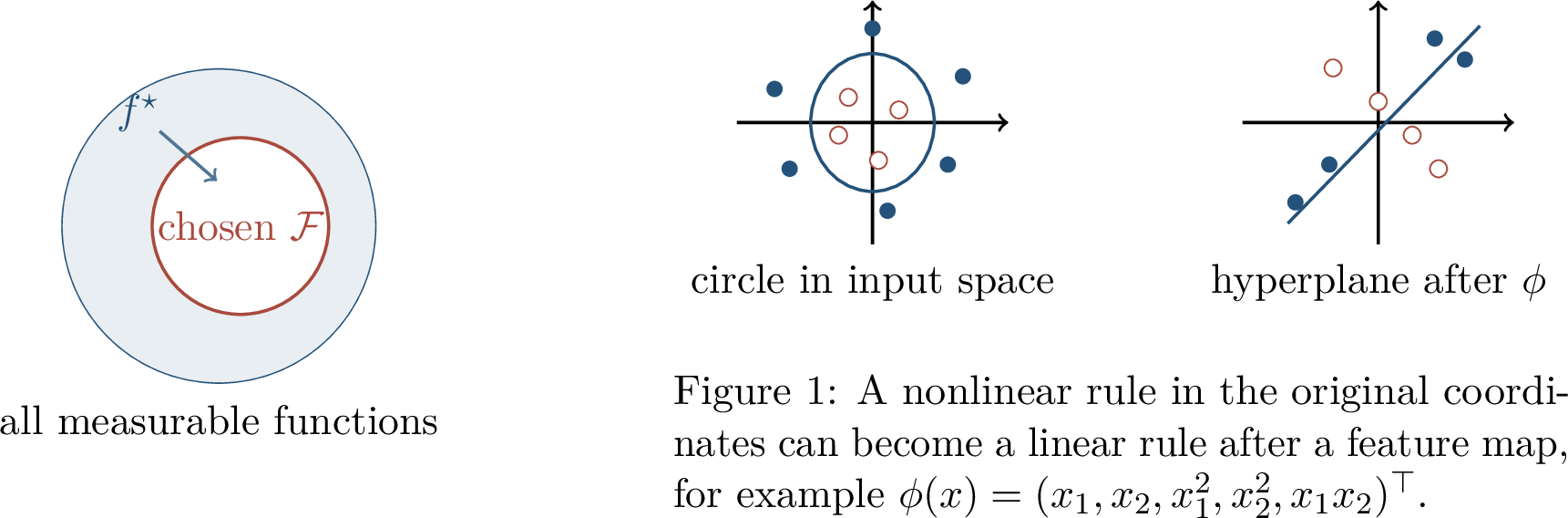
The approximation problem may now be stated abstractly. Given a target function \(g\) and a network class \(\mathcal{F}_{L,m}\) of depth \(L\) and width \(m\), bound \[\inf_{f\in\mathcal{F}_{L,m}}\left\lVert f-g \right\rVert\] in a norm appropriate to the learning task, such as \(L^\infty\) on a compact set or \(L^2(\mu)\) under a data distribution. Qualitative theory asks whether the infimum can be made arbitrarily small. Quantitative theory asks how the error decreases as width, depth, or parameter count grows.
The choice of norm changes the meaning of approximation. Uniform approximation controls the error at every point of a compact set; it is strong and natural in classical analysis. \(L^2(\mu)\) approximation controls average squared error under the data distribution; it is weaker, but closer to statistical risk. A function may be a good \(L^2(\mu)\) approximation while behaving poorly on regions that have negligible probability. This distinction will reappear in later chapters on generalization, robustness, and distribution shift.
1.1.8 Network Classes and Activation Functions↩︎
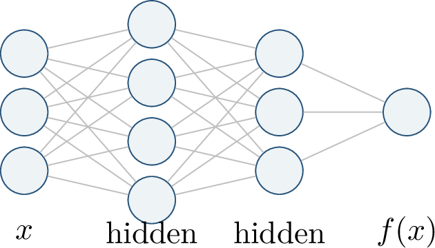
A feedforward network is a composition of affine maps and coordinatewise nonlinearities. If \(n_0=d\) and \(n_L\) is the output dimension, a depth-\(L\) network computes \[f(x;W)=\sigma_L\!\left( W_L\sigma_{L-1}\!\left(\cdots\sigma_1(W_1x+b_1)\cdots\right)+b_L \right),\] where \(W_\ell\in\R^{n_\ell\times n_{\ell-1}}\), \(b_\ell\in\R^{n_\ell}\), and each \(\sigma_\ell\) acts coordinatewise. The width is typically \(\max_\ell n_\ell\), and \(W\) is used as shorthand for all weights and biases.
This formula should be read from the inside out. The first affine map \(x\mapsto W_1x+b_1\) creates \(n_1\) learned features from the input. The activation then applies the same scalar nonlinearity to each coordinate. The next layer repeats this operation, using the previous learned features as its new input. Thus a deep network is not merely a large linear model; it is an iterated construction of features. Depth measures the number of nonlinear feature transformations, while width measures the number of coordinates available at a layer.
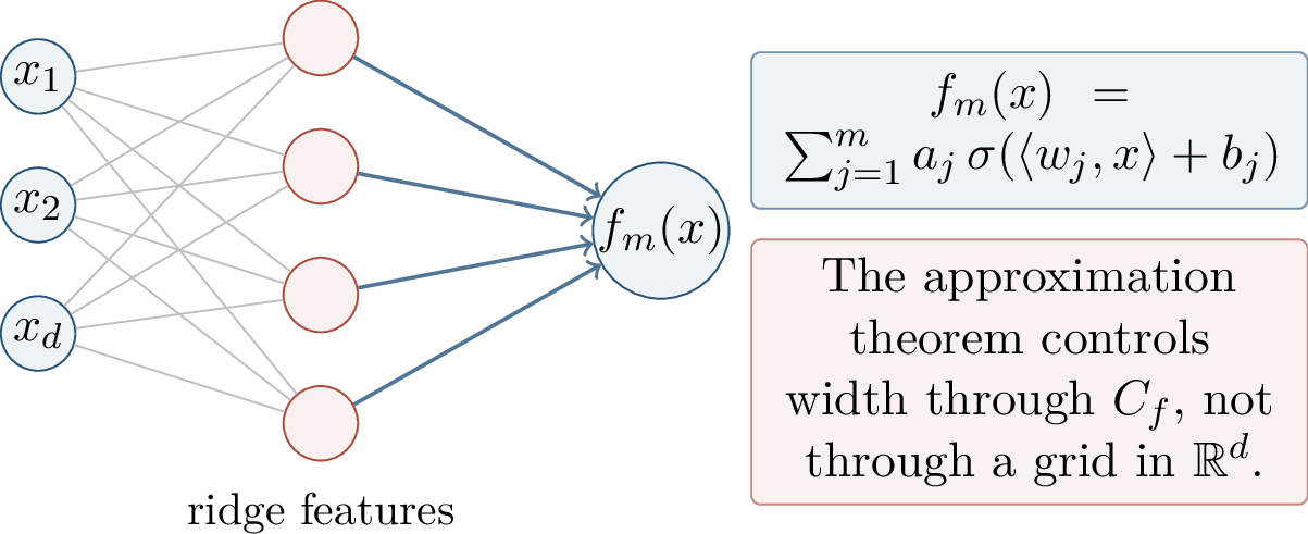
The central shallow architecture in this chapter is the depth-two ridge-function class \[f_m(x)=\sum_{j=1}^m a_j\,\sigma(\left\langle w_j,x \right\rangle+b_j).\] Each hidden unit forms an affine feature \(\left\langle w_j,x \right\rangle+b_j\), applies a nonlinearity, and the output layer adds the resulting features.
Why a Nonlinearity Is Essential If every activation is the identity map, then the composition of affine maps is again affine. Indeed, \[W_2(W_1x+b_1)+b_2=(W_2W_1)x+(W_2b_1+b_2),\] and the same calculation repeats through all layers. Such a network cannot represent curved decision boundaries or nonlinear regression functions. The activation function is therefore the source of expressive power.
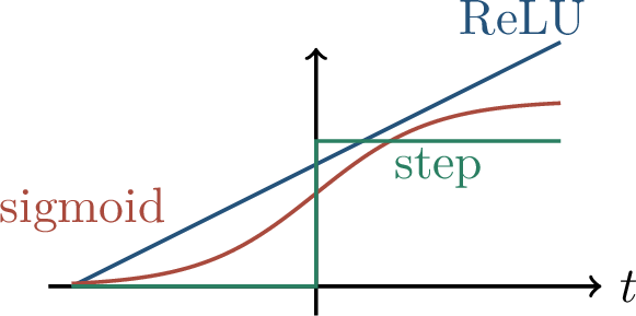
The choice of activation matters. Standard examples include \[\relu(t)=\max\{t,0\},\qquad s(t)=\frac{1}{1+e^{-t}},\qquad H(t)=\mathbf{1}_{\{t\ge0\}},\qquad c(t)=\cos(t).\] ReLU activations give continuous piecewise-linear functions and are dominant in modern practice. Sigmoid and threshold activations appear naturally in classical approximation proofs. Cosine activations connect network approximation with Fourier analysis.
The same approximation theorem may look different for different activations. For threshold functions, one can literally build step approximations. For sigmoids, a steep sigmoid approximates a threshold, so many threshold-based arguments have smooth analogues. For ReLU, the basic geometric object is a hinge rather than a jump. A finite ReLU network is continuous, and in one dimension it is piecewise linear. In higher dimensions, the hinges occur along hyperplanes and their compositions create polyhedral regions.
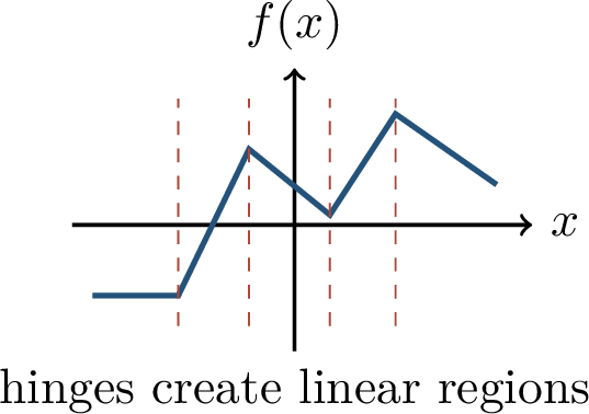
ReLU networks compute continuous piecewise-linear functions. In one dimension, each ReLU contributes a hinge. In higher dimensions, the affine thresholds \(\left\langle w_j,x \right\rangle+b_j=0\) partition the input space by hyperplanes, and depth composes these partitions.
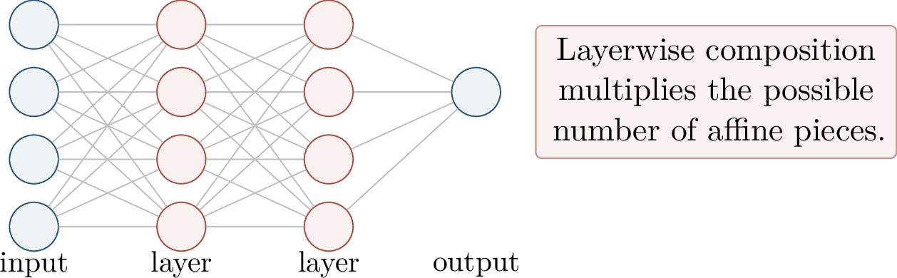
This remark is often the most useful way to remember ReLU expressivity. A single ReLU unit \(\relu(\left\langle w,x \right\rangle+b)\) is affine on each side of the hyperplane \(\left\langle w,x \right\rangle+b=0\). A sum of such units creates a piecewise-affine surface with many linear pieces. A deeper network feeds one piecewise-affine map into another, so the number and arrangement of linear regions can grow rapidly with depth. Later chapters will use this observation to discuss depth separation.
1.1.9 Universal Approximation↩︎
Definition 1.3 (Universal Approximator). Let \(K\subset\R^d\) be compact. A function class \(\mathcal{F}\subset C(K)\) is a universal approximator if, for every \(g\in C(K)\) and every \(\varepsilon>0\), there exists \(f\in\mathcal{F}\) such that \[\sup_{x\in K}\left\lvert f(x)-g(x) \right\rvert\le \varepsilon.\]
This is a density statement in the uniform norm. It says that the closure of \(\mathcal{F}\) is all of \(C(K)\), but it says nothing yet about the size of the network, the numerical values of the parameters, or how an algorithm might discover them. The compactness of \(K\) is important. Uniform approximation on all of \(\R^d\) is usually too strong without imposing growth or decay conditions. Compact domains allow continuous functions to be uniformly continuous, which is the basic analytic fact behind many constructive proofs.
Theorem 1.1 (Stone-Weierstrass). Let \(K\) be compact and let \(\mathcal{A}\subset C(K)\) be a subalgebra that contains the constants and separates points: whenever \(x\ne y\) in \(K\), there is \(h\in\mathcal{A}\) with \(h(x)\ne h(y)\). Then \(\mathcal{A}\) is dense in \(C(K)\) under the uniform norm.
The reference notes state the same classical lens in a slightly more flexible form: a class of continuous functions that is closed under vector-space operations and multiplication, separates points, and has a nonzero function at each point is universal. Polynomials satisfy these hypotheses on compact subsets of \(\R^d\), so polynomials with unbounded degree can uniformly approximate every continuous function. Neural networks offer a different dense family, one whose elements are built from ridge functions.
Stone-Weierstrass is not a neural-network theorem, but it gives the conceptual template. It says that a sufficiently rich algebra of simple functions is dense in \(C(K)\). Neural networks are not usually handled by directly checking the algebra hypotheses for a fixed finite-width class. Instead, one shows that finite sums of ridge functions are rich enough to separate continuous linear functionals on \(C(K)\), or one constructs approximations from localized units. Both viewpoints lead to the same qualitative conclusion: finite neural networks can approximate arbitrary continuous targets on compact sets when width is allowed to grow.
Theorem 1.2 (Depth-Two Universal Approximation). Let \(\sigma:\R\to\R\) be continuous and non-polynomial. For every compact \(K\subset\R^d\), the depth-two classes \[\mathcal{F}_m = \left\{x\mapsto \sum_{j=1}^m a_j\,\sigma(\left\langle w_j,x \right\rangle+b_j)\right\}\] are dense in \(C(K)\) as \(m\to\infty\).
One classical meta-theorem, associated with the work of Cybenko, Hornik, and later refinements by Leshno, Lin, Pinkus, and Schocken, is that many non-polynomial activations produce universal shallow networks. For sigmoid-like activations, a common condition is \[\lim_{z\to-\infty}\sigma(z)=0, \qquad \lim_{z\to+\infty}\sigma(z)=1,\] which allows hidden units to approximate threshold tests. ReLU is not bounded like a sigmoid, but it also yields universal approximation.
The phrase “as \(m\to\infty\)” means that for each target accuracy one may choose a sufficiently large number of hidden units. The theorem does not assert that one fixed \(m\) works for all targets. Nor does it provide a dimension-free rate. The result is best understood as an expressive baseline: the architecture is not fundamentally incapable of representing continuous functions. The rest of approximation theory asks how expensive this representation is.
1.1.9.1 A One-Dimensional Construction
The most transparent proof idea is local approximation. Approximate a continuous function by a simple piecewise function, then build the pieces from hidden units and add them in the output layer. In one dimension the construction is especially explicit: a threshold unit \(H(x-t)\) turns on when the input crosses the breakpoint \(t\). A linear combination of such units can therefore create a step function whose jumps occur at prescribed grid points.
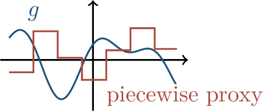
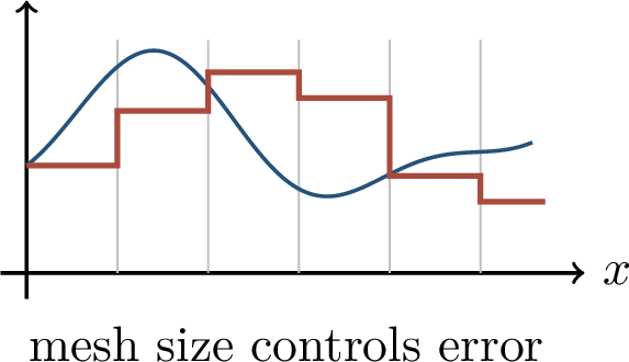
Let \(g:[0,1]\to\R\) be \(\rho\)-Lipschitz and let \(H(t)=\mathbf{1}_{\{t\ge0\}}\). For every \(\varepsilon>0\), there is a depth-two threshold network \[\widehat g(x) = g(0)+\sum_{i=1}^{m-1} \bigl(g(x_i)-g(x_{i-1})\bigr)H(x-x_i)\] with \(m\le \lceil \rho/\varepsilon\rceil+1\) grid cells such that \[\sup_{x\in[0,1]}\left\lvert g(x)-\widehat g(x) \right\rvert\le \varepsilon.\]
Proof. Partition \([0,1]\) into intervals whose length is at most \(\varepsilon/\rho\), with the obvious simplification when \(\rho=0\). Let \(x_i\) be the grid points and define the coefficients by telescoping increments: \[a_1=g(x_1)-g(0),\qquad a_i=g(x_i)-g(x_{i-1})\quad (i\ge2).\] On the interval containing \(x\), the sum telescopes so that \(\widehat g(x)\) equals the value of \(g\) at the left grid point. The Lipschitz condition gives \[\left\lvert g(x)-\widehat g(x) \right\rvert \le \rho\,\left\lvert x-x_i \right\rvert \le \varepsilon.\] ◻
The proof is worth unpacking. The first term \(g(0)\) sets the initial height. The coefficient multiplying \(H(x-x_i)\) is the change in the target value when moving from \(x_{i-1}\) to \(x_i\). When \(x\) passes the breakpoint \(x_i\), that change is added to the output. Thus the network stores the values of \(g\) on the grid by storing their increments. Lipschitz continuity then converts mesh size into approximation error.
From Thresholds to Smooth Activations The threshold construction is discontinuous, while the target \(g\) is continuous. This is not a contradiction: uniform approximation allows the approximant to have jumps as long as its values stay close to \(g\). If a smooth sigmoid is used instead of \(H\), one can approximate each threshold by a steep sigmoid. ReLU networks use a related idea with piecewise-linear “ramps” rather than jumps.
1.1.9.2 The Multivariate Cost
Uniform continuity extends the idea to \([0,1]^d\), but at a price.
Let \(g:[0,1]^d\to\R\) be uniformly continuous. Suppose that \(\delta>0\) is chosen so that \[\left\lVert x-y \right\rVert_\infty\le\delta \quad\Longrightarrow\quad \left\lvert g(x)-g(y) \right\rvert\le \varepsilon.\] If \([0,1]^d\) is partitioned into rectangles of side length at most \(\delta\), then there is a piecewise-constant function \(f\) on the partition such that \[\sup_{x\in[0,1]^d}\left\lvert g(x)-f(x) \right\rvert\le\varepsilon.\]
Proof. For each cell \(R_i\), choose a point \(x_i\in R_i\) and set the value on the cell to \(g(x_i)\). If \(x\in R_i\), then \(\left\lVert x-x_i \right\rVert_\infty\le\delta\), so \(\left\lvert g(x)-g(x_i) \right\rvert\le\varepsilon\). ◻
The number of cells is approximately \(\delta^{-d}\). Thus the construction is essentially a lookup table. It proves universality, but it also reveals the curse of dimensionality: arbitrary continuous functions require a number of local pieces that grows exponentially with \(d\).
For a \(\rho\)-Lipschitz function on \([0,1]^d\), choosing \(\delta\approx\varepsilon/\rho\) gives on the order of \((\rho/\varepsilon)^d\) grid cells. This scaling is not a peculiarity of the proof; it reflects the fact that continuity alone imposes very little global structure. A target may vary independently in many small regions of the cube. Without additional assumptions, a method that controls the function uniformly must inspect all those regions.
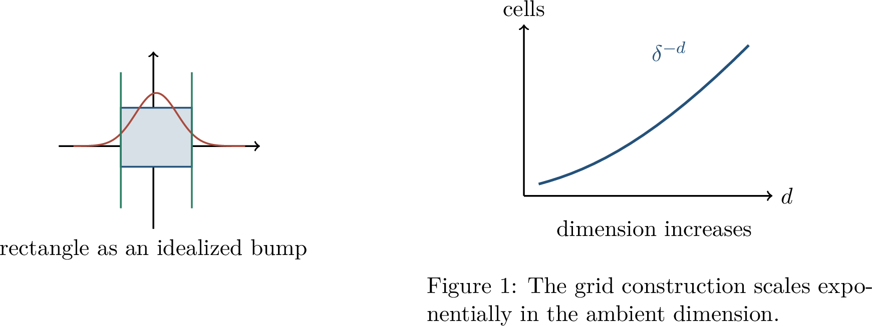
The monograph also describe why cosine activations are convenient in a multivariate construction. Products of one-dimensional oscillatory factors can be rewritten as sums of ridge functions: \[\prod_{j=1}^d \cos(t_j) = 2^{-d}\sum_{\eta\in\{\pm1\}^d} \cos(\left\langle \eta,t \right\rangle).\] This identity is the higher-dimensional version of \[\cos(x)\cos(y)=\frac{\cos(x+y)+\cos(x-y)}{2}.\] It explains how a product bump can be represented using sums of functions of linear combinations. The construction is mathematically useful, but unless the target has additional structure it still inherits the grid cost.
This point is a useful warning. A clever identity may convert a local multivariate object into a sum of ridge functions, but if the number of local objects is exponential, the total representation remains exponential. To obtain dimension-friendly rates one must use structure beyond continuity: Fourier decay, compositional form, low-dimensional geometry, sparsity, or some other constraint that rules out arbitrary independent variation in every grid cell.
Universality gives existence, not efficient size. It does not say that the network is small, that gradient descent can find the approximating parameters, or that a predictor trained from finite data will generalize. Smoothness assumptions, Besov-type regularity, manifold structure, or spectral structure can lead to better rates than a raw grid, but continuity alone is too weak.
Thus universal approximation should be read as a necessary sanity check rather than a complete theory of deep learning. It rules out a basic expressivity obstruction. It does not explain why practical architectures with finite size work well on high-dimensional data. Barron theory is one answer to this quantitative gap for a particular spectral class.
1.1.10 Barron Theory↩︎
Barron’s theorem shifts attention from arbitrary continuous functions to a structured class defined through Fourier decay. For an integrable function \(f:\R^d\to\R\), use the Fourier convention \[\require{physics} \begin{align} \widehat f(\omega) &= \int_{\R^d} e^{-2\pi i\left\langle \omega,x \right\rangle} f(x)\,\dd x,\\ f(x) &= \int_{\R^d} e^{2\pi i\left\langle \omega,x \right\rangle}\widehat f(\omega)\,\dd\omega, \end{align}\] under the usual technical conditions ensuring inversion. Frequencies encode directions and oscillation scales. Moving mass farther from the origin corresponds to more rapid oscillation.
The key change of perspective is this: rather than asking only whether a continuous function can be approximated, Barron theory asks whether the function has a Fourier representation whose mass is concentrated at moderate frequencies. A high-dimensional grid treats the domain as a collection of small boxes. Fourier analysis treats the target as a superposition of waves. Ridge functions are compatible with this second viewpoint because a ridge feature \(\sigma(\left\langle w,x \right\rangle+b)\) depends on \(x\) only through one direction. This directional structure is what allows shallow networks to avoid an explicit grid for certain function classes.
Definition 1.4 (Barron Seminorm). A convenient Barron quantity is \[\require{physics} B(f)=\int_{\R^d}\left\lVert \omega \right\rVert_2\,\left\lvert \widehat f(\omega) \right\rvert\,\dd\omega.\] The Barron class consists of functions for which \(B(f)<\infty\).
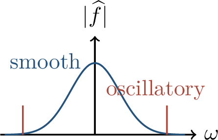
This quantity is closely related to the \(L^1\) norm of the Fourier transform of the gradient: up to Fourier-convention constants, \[B(f)\simeq \left\lVert \widehat{\grad f} \right\rVert_1.\] Low-frequency functions tend to have smaller Barron seminorm, while highly oscillatory functions pay through the factor \(\left\lVert \omega \right\rVert_2\).
The word “seminorm” is deliberate. Depending on the precise function space and Fourier convention, constants or other low-frequency components may require separate treatment. For the purposes of this chapter, the important feature is the weighted Fourier first moment: frequency mass far from the origin is expensive. This is a structural assumption, not a consequence of continuity. Many continuous functions do not have finite Barron seminorm.
Theorem 1.3 (Barron Approximation). Let \(K\subset\R^d\) be bounded and let \(\mu\) be a probability measure on \(K\). If \(B(f)<\infty\), then for every \(k\ge1\) there exists a depth-two network \[f_k(x)=\sum_{j=1}^k a_j\,\sigma(\left\langle w_j,x \right\rangle+b_j)\] such that \[\require{physics} \int_K\left\lvert f(x)-f_k(x) \right\rvert^2\,\dd\mu(x) \le \frac{C\,B(f)^2}{k},\] where \(C\) depends on normalization choices and the bounded domain, but not on the ambient dimension through a grid factor.
In the reference notes this is framed as follows: for appropriate depth-two networks with \(k\) hidden units, \[\require{physics} \int \left\lvert f(x)-g(x) \right\rvert^2\,\dd x \le \frac{4C_f}{k}, \qquad C_f=\left(\int \left\lVert \omega \right\rVert\,\left\lvert \widehat f(\omega) \right\rvert\,\dd\omega\right)^2.\] The exact constants depend on conventions, but the message is robust: once the spectral first moment is controlled, the approximation rate is Monte Carlo-like rather than grid-like.
Several qualifications are essential. First, the theorem is an approximation result: it asserts the existence of a network \(f_k\), not that a particular training algorithm will find it. Second, the hidden constant is not literally free of dimension in all senses; it may depend on the radius of the domain, the normalization of the Fourier transform, the activation, and how the Barron quantity is defined. What the theorem avoids is the explicit \(\delta^{-d}\)-type grid count for the function class under consideration. Third, the conclusion is in squared \(L^2(\mu)\) error. Thus the corresponding \(L^2\) error scales like \(k^{-1/2}\), the same rate one expects from Monte Carlo averaging.
1.1.10.1 Infinite Width and Sampling
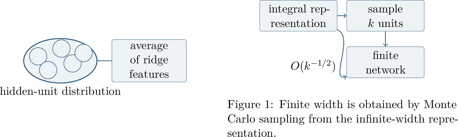
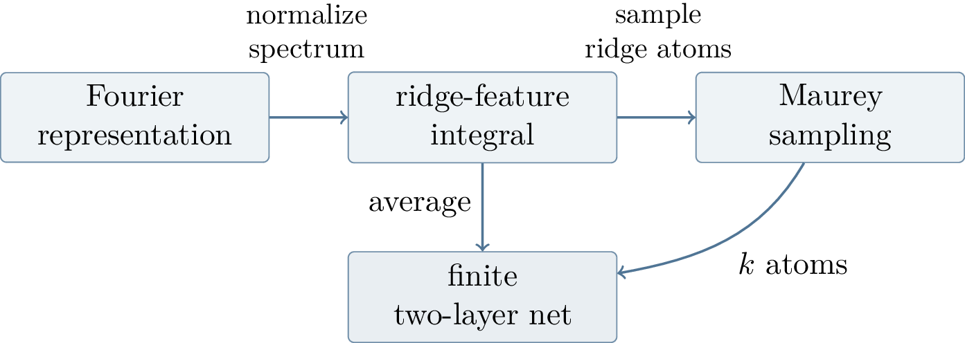
The proof architecture has two steps. First, Fourier inversion is rewritten as an integral over ridge features. Schematically, \[f(x)\approx \E_{\theta\sim\nu} \bigl[a(\theta)\,\varphi_\theta(x)\bigr], \qquad \varphi_\theta(x)=\sigma(\left\langle w,x \right\rangle+b).\] This is an infinite-width network: instead of a finite sum over hidden units, it averages over a distribution of hidden units. Second, one samples \(k\) hidden units from this distribution and uses their empirical average.
The notation is schematic because different activations require different ridge-feature representations. For sigmoidal activations, Barron’s original argument expresses Fourier components through superpositions of sigmoids. For other activations, one often works with related integral representations. The common structure is that the target lies in the closure of a convex or signed convex hull of bounded ridge features. Once such an infinite representation is available, the finite-width approximation is a sampling problem.
The elementary Hilbert-space tool behind this sampling step is Maurey’s lemma.
Lemma 1.1 (Maurey-Type Sparsification). Let \(\mathcal{H}\) be a Hilbert space and let \(S\subset\mathcal{H}\) satisfy \[\sup_{v\in S}\left\lVert v \right\rVert^2\le M^2.\] If \(h\in\operatorname{conv}(S)\), then for every \(k\) there exist \(v_1,\ldots,v_k\in S\) such that \[\left\|h-\frac{1}{k}\sum_{j=1}^k v_j\right\|^2 \le \frac{M^2}{k}.\]
Proof. Since \(h\in\operatorname{conv}(S)\), choose a random vector \(V\) supported on \(S\) with \(\E V=h\). Let \(V_1,\ldots,V_k\) be independent copies and set \(\overline{V}_k=k^{-1}\sum_{j=1}^kV_j\). Then \[\begin{align} \E\left\lVert h-\overline{V}_k \right\rVert^2 &= \frac{1}{k^2}\E\left\lVert \sum_{j=1}^k(h-V_j) \right\rVert^2\\ &= \frac{1}{k}\E\left\lVert h-V \right\rVert^2 \le \frac{1}{k}\E\left\lVert V \right\rVert^2 \le \frac{M^2}{k}. \end{align}\] Therefore at least one sampled average achieves the displayed bound. ◻
A version with signed or general coefficients follows by applying the same argument after normalizing the total variation of the coefficient measure. This is why the Barron proof can convert an infinite mixture of ridge features into a finite network whose error decays like \(1/k\) in squared \(L^2\) norm.
The proof contains the entire Monte Carlo mechanism. The random average \(\overline{V}_k\) is an empirical approximation to its mean \(h\). Independence causes the cross terms in the squared norm to vanish, leaving a variance term of size \(1/k\). Since the expected error is at most \(M^2/k\), at least one realization must achieve that bound. In the neural-network setting, the vectors \(V_j\) are ridge features viewed as elements of a Hilbert space such as \(L^2(\mu)\), and the sampled average becomes a finite hidden layer.
Reading the Rate Correctly The Maurey bound is a squared-norm bound. If \(\|h-k^{-1}\sum_j v_j\|^2\le M^2/k\), then the norm error is at most \(M/\sqrt{k}\). Barron’s theorem is commonly stated as a squared \(L^2\) error of order \(1/k\). This is why Figure [fig:ch01-finite-sampling] labels the direct sampling path by \(O(k^{-1/2})\): it refers to the \(L^2\) norm rather than its square.
Example 1.1 (Low and High Frequencies). For a unit direction \(u\), \[f(x)=\cos(2\pi\,u^\top x)\] has Fourier mass concentrated at \(\pm u\), so its Barron quantity scales with \(\left\lVert u \right\rVert\). By contrast, \[g(x)=\cos(2\pi q\,u^\top x)\] has mass at \(\pm q u\), and its Barron quantity scales with \(q\left\lVert u \right\rVert\). High-frequency oscillation is therefore harder for shallow Barron approximation.
This example should not be interpreted as saying that a high-frequency function cannot be represented by a shallow network. A single sinusoid in one direction has a simple structure. The point is quantitative: the Barron seminorm grows with the frequency scale, so the theorem permits a worse approximation constant. The theorem rewards spectral concentration near the origin and penalizes rapid oscillation.

1.1.11 Connections and Limits↩︎
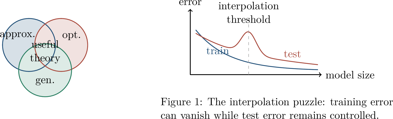
Approximation theorems are necessary but not sufficient explanations of deep learning. They tell us that a good network exists; optimization asks whether training finds one; generalization asks whether the trained network predicts beyond the sample. A classical strategy is to control all three using a shared notion of model complexity, but modern overparameterized networks often fit the training data exactly and still generalize well. This interpolation phenomenon is not explained by universal approximation alone.
The distinction is important enough to state plainly. A universal approximation theorem is not a training theorem. It does not say that empirical risk minimization is computationally feasible, that gradient descent avoids bad regions of the landscape, or that the discovered parameters have any special stability property. Likewise, an approximation theorem is not a generalization theorem. It does not control the gap between \(\widehat{\mathcal{R}}_S\) and \(\mathcal{R}\). These questions require additional tools: optimization dynamics, concentration, capacity measures, stability, implicit regularization, and distributional assumptions.
Barron theory is closely related to random features. If the hidden parameters \((w_j,b_j)\) are sampled and fixed, then \[f_k(x)=\frac{1}{k}\sum_{j=1}^k a_j\sigma(\left\langle w_j,x \right\rangle+b_j)\] is a random feature model in which only output weights may be learned. Wide networks near random initialization can also behave like kernel methods through the neural tangent kernel (NTK), while mean-field regimes study the evolution of the distribution of hidden units. These viewpoints keep the integral representation but assign different roles to training.
This connection also clarifies the role of width. In the Barron proof, width is the number of sampled ridge features used to approximate an infinite-width integral. In random feature models, width is the number of random basis functions made available to the linear output layer. In neural tangent kernel limits, width controls how closely training follows a linearized kernel regime. The same architectural parameter therefore appears in several theories, but it does not have the same meaning in all of them.
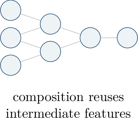
Depth introduces another kind of structure. Universal approximation by shallow networks says that width alone is enough in principle, but it does not say that the representation is succinct. There are function families with compact deep representations that require exponentially many units for certain shallow architectures. Depth supports compositional reuse of intermediate features.
The approximation results in this chapter therefore leave open a central theme of deep learning theory: efficiency. A shallow network may approximate a function eventually, but a deep network may represent the same function with far fewer units when the target has compositional structure. Later depth separation results make this statement precise for carefully constructed function families; see, for example, the depth-separation literature represented by Telgarsky’s construction and related work [6].
There is also a complementary width-versus-depth result. For ReLU networks with unbounded depth, narrow architectures can still be universal in \(L^p\) senses. A representative modern statement is that, for functions \([0,1]^{d_x}\to\R^{d_y}\), widths on the order of \(\max\{d_x+1,d_y\}\) can be sufficient in suitable settings, and related results characterize minimum widths. Such theorems show that depth can compensate for width, but they may remain nonconstructive or inefficient for actual training.
For this reason, one should separate three statements that are sometimes conflated. First, a class may be universal: it can approximate any continuous target if allowed to grow. Second, a class may approximate a structured target efficiently: the required size grows slowly with accuracy and dimension. Third, a training algorithm may find such an efficient approximation from data. The first statement is the subject of universal approximation. The second is the subject of quantitative approximation theory, including Barron-type results. The third belongs to optimization and statistical learning theory.
The results in this chapter are mainly approximation results. The parameters constructed in the proofs need not be found by gradient descent. Worst-case continuous targets can be exponentially hard. Small training error does not imply robustness, interpretability, fairness, transfer, or good performance under distribution shift. Finally, real data may have structure not captured by IID assumptions or by Fourier smoothness alone.
The limitations are not defects of the theory; they are boundary markers. They tell us which questions have been answered and which have merely been exposed. Approximation theory supplies a language for discussing expressive power. It does not by itself explain optimization, sample complexity, or the remarkable empirical behavior of large trained networks. The following chapters will add these missing pieces one at a time.
1.1.12 Summary and Further Reading↩︎
Universal approximation tells us that neural networks are expressive: with unbounded width, shallow networks can approximate broad classes of continuous functions. The constructive picture also warns us that arbitrary continuous functions may require exponentially many local pieces in high dimensions. Barron’s theorem gives a more refined message: for functions with controlled spectral first moment, shallow networks achieve a dimension-friendly Monte-Carlo-type rate. The proof proceeds by viewing an infinite-width network as an integral over ridge features and then sparsifying that integral with Maurey’s lemma.
The chapter has developed three levels of understanding. At the qualitative level, neural networks are universal approximators on compact domains. At the constructive level, one can approximate by local pieces, but the naive multivariate construction reveals an exponential grid cost. At the structural level, Barron theory identifies a class for which shallow networks avoid this grid cost because the target has controlled Fourier first moment. These levels should be kept distinct: universality, constructive approximation, and dimension-friendly rates are different claims.
For later use, the main conceptual lesson is that approximation theory studies the existence and size of good networks. It does not determine which network a training algorithm selects, nor whether finite-sample training gives good test performance. Those questions motivate the next parts of the monograph.
For classical universal approximation, see Cybenko [3] and Hornik [28]. For the quantitative spectral result emphasized in this chapter, see Barron [4]. For broader background on neural-network modeling and statistical learning, see Goodfellow, Bengio, and Courville [29] and Shalev-Shwartz and Ben-David [2]. For later approximation results involving depth and ReLU networks, see Telgarsky [6] and Yarotsky [7].
1.1.13 The Three Questions of the Chapter↩︎
Chapter 1 ended with a positive approximation result: under a spectral first-moment condition, a two-layer neural network can approximate a function on a bounded domain with error of order \(m^{-1/2}\), where \(m\) is the number of hidden units. The striking feature of this theorem is that the bound is controlled by a function norm, \[\require{physics} C_f = 2\pi\int_{\R^d}\left\lVert \omega \right\rVert\left\lvert \widehat f(\omega) \right\rvert\,\dd \omega,\] rather than by a grid resolution in \(\R^d\). This chapter takes that result apart and then asks what it does and does not explain.
The distinction is subtle but foundational. A classical universal approximation theorem tells us that a sufficiently large neural network can approximate every continuous function on a compact set. Such a statement is qualitative: it guarantees density, but it does not by itself tell us whether the required network size is moderate, enormous, or exponentially large in the ambient dimension. Barron’s theorem [4] is of a different flavor. It says that a particular spectral regularity condition leads to a quantitative width-error tradeoff. The theorem therefore converts an analytic property of the target function into a statement about the size of a shallow network.
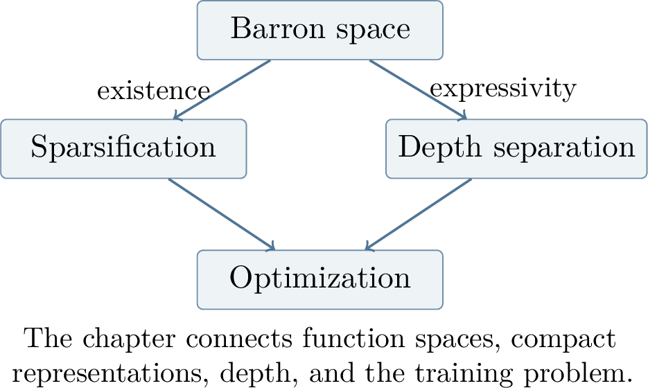
There are three guiding questions. First, when can a shallow network avoid the curse of dimensionality? Second, when does depth give an exponential representational advantage over shallower networks? Third, even if a compact representation exists, can a training algorithm find it?
These questions should be kept separate. The first is an approximation question about a function class. The second is an expressivity comparison between architectures. The third is an algorithmic question about empirical risk minimization in parameter space. Many confusions in deep-learning theory arise from moving too quickly from one question to another. A small network may exist without being easy to train; a function may be easy for a deep architecture and hard for a shallow one; and an optimization result may rely on overparameterization in a regime where the learned function is very different from the compact representation suggested by approximation theory.
A useful mental model is a shallow network whose hidden units are ridge features: \[f_m(x)=\sum_{j=1}^m a_j\,\sigma(\left\langle w_j,x \right\rangle+b_j).\] The Barron theorem does not say that every continuous function is easy. It says that functions with controlled spectral first moment can be represented by averaging a modest number of ridge atoms. The width is governed by \(C_f\), not by a full tensor-product discretization of the input domain.
The word “ridge” means that each hidden unit sees the input through the projection \(\left\langle w_j,x \right\rangle\). A single unit is a one-dimensional nonlinear function pulled back along a direction in \(\R^d\). The surprising part of Barron’s theorem is not that ridge functions are expressive in principle, but that for a structured spectral class an average of such atoms can approximate a high-dimensional target without partitioning the whole cube or ball into tiny boxes.
The main chain in this chapter is: \[\text{Fourier control} \Longrightarrow \text{Barron representation} \Longrightarrow \text{sparse shallow network},\] and, separately, \[\text{module composition} \Longrightarrow \text{many linear regions} \Longrightarrow \text{depth separation}.\] The final part of the chapter returns to optimization. Approximation and expressivity are existence statements. Training is an algorithmic problem.
How to Read This Chapter The first two sections study shallow approximation: an analytic condition on \(f\) gives an infinite mixture of simple atoms, and a sparsification lemma turns that mixture into a finite network. The third section studies depth: repeated composition can produce exponentially many oscillations using only a linear number of modules. The last section then explains why neither statement is automatically an optimization theorem.
1.1.14 Barron Representations↩︎
We work on the unit ball \[B_2^d=\{x\in\R^d:\left\lVert x \right\rVert\le 1\}.\] Throughout this section the Fourier transform is normalized so that \[\require{physics} f(x)=\int_{\R^d} e^{2\pi i\left\langle \omega,x \right\rangle}\widehat f(\omega)\,\dd\omega.\] This convention fixes the \(2\pi\) constants in the definition of \(C_f\). Changing the Fourier convention changes these constants but not the main message: the relevant quantity is the first moment of the magnitude of the Fourier transform. The restriction to \(B_2^d\) is also not essential. It is used to normalize the range of the one-dimensional projections \(\left\langle \omega,x \right\rangle\), so that thresholds can be compared on a bounded domain.
For a real-valued function \(f\), write the complex phase as \[\widehat f(\omega)=\left\lvert \widehat f(\omega) \right\rvert e^{2\pi i\theta(\omega)}.\] Taking the real part of the Fourier inversion formula gives \[\require{physics} f(x) = \int_{\R^d} \cos\!\bigl(2\pi\left\langle \omega,x \right\rangle+2\pi\theta(\omega)\bigr) \left\lvert \widehat f(\omega) \right\rvert\,\dd\omega . \label{eq:ch2-real-fourier}\tag{1}\]
Definition 1.5 (Barron spectral complexity). The Barron spectral complexity of \(f\), for the Fourier convention above, is \[\require{physics} C_f = 2\pi\int_{\R^d}\left\lVert \omega \right\rVert\left\lvert \widehat f(\omega) \right\rvert\,\dd\omega .\] When \(C_f<\infty\), the high-frequency mass of \(f\) has a finite first moment.
The phrase “first moment” is important. Low-frequency mass is cheap, while mass far from the origin is expensive because it produces rapid oscillation. This is the mechanism by which the theorem can avoid explicit dimension counting: dimension enters through the distribution of Fourier mass, not through a grid of side length \(\varepsilon^{-1}\) in each coordinate.
It is useful to compare \(C_f\) with two more familiar quantities. The integral \(\require{physics} \int \left\lvert \widehat f(\omega) \right\rvert\,\dd\omega\), when finite, controls the uniform size of \(f\) through Fourier inversion. The stronger integral \(\require{physics} \int \left\lVert \omega \right\rVert\left\lvert \widehat f(\omega) \right\rvert\,\dd\omega\) controls how much variation is created when \(x\) moves inside the domain. In this sense \(C_f\) is a Fourier-side Lipschitz-type complexity: it penalizes the total amount of directional oscillation available to \(f\).
Spectral Complexity Is Not Dimension Alone A function in a large ambient dimension can have small Barron complexity if its Fourier mass is concentrated near low-frequency directions. Conversely, even in low dimension, a rapidly oscillating function can have large \(C_f\). The norm therefore measures structure of the function, not merely the number of coordinates.
1.1.14.1 From Fourier Phase to Halfspace Atoms
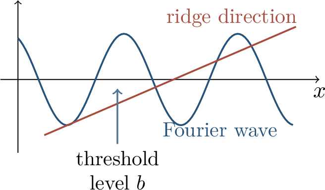
The starting point is to subtract the constant value \(f(0)\). From 1 , \[\require{physics} \begin{align} f(x)-f(0) &= \int_{\R^d} \Bigl[ \cos(2\pi\left\langle \omega,x \right\rangle+\phi_\omega) -\cos(\phi_\omega) \Bigr]\left\lvert \widehat f(\omega) \right\rvert\,\dd\omega , \end{align}\] where \(\phi_\omega=2\pi\theta(\omega)\). The fundamental theorem of calculus in the scalar variable \(t=\left\langle \omega,x \right\rangle\) yields \[\require{physics} \cos(2\pi t+\phi_\omega)-\cos(\phi_\omega) = \int_0^t -2\pi\sin(2\pi b+\phi_\omega)\,\dd b .\] On \(B_2^d\), \(\left\lvert t \right\rvert\le \left\lVert \omega \right\rVert\). Thus the amount of signed mass created by frequency \(\omega\) is bounded by \[2\pi\left\lVert \omega \right\rVert\left\lvert \widehat f(\omega) \right\rvert.\] Integrating over \(\omega\) is exactly where \(C_f\) appears.
The subtraction of \(f(0)\) is not a trick to remove an inconvenient constant; it isolates the part of \(f\) that is created by directional variation. A constant function can be represented by the output bias of a network, so the interesting question is how to represent changes away from the origin. For a fixed frequency \(\omega\), the scalar variable \(t=\left\langle \omega,x \right\rangle\) moves in an interval of length at most \(2\left\lVert \omega \right\rVert\) on \(B_2^d\). The fundamental theorem of calculus expresses the change of the cosine along this interval as an integral over threshold levels \(b\). Each threshold level corresponds to a halfspace atom.
Suppose \(f\) is real-valued on \(B_2^d\) and \(C_f<\infty\). Then \(f-f(0)\) admits an infinite-width signed ridge representation by halfspace atoms. One convenient unnormalized form is \[\require{physics} f(x)-f(0) = \int_{\R^d}\int_{-\left\lVert \omega \right\rVert}^{\left\lVert \omega \right\rVert} \widetilde{a}(\omega,b)\, \mathbf{1}\{\left\langle \omega,x \right\rangle\ge b\}\,\dd b\,\dd\omega , \qquad x\in B_2^d,\] with a signed density satisfying \[\require{physics} \int_{\R^d}\int_{-\left\lVert \omega \right\rVert}^{\left\lVert \omega \right\rVert} \left\lvert \widetilde{a}(\omega,b) \right\rvert\,\dd b\,\dd\omega \le 2 C_f.\] Equivalently, after normalizing the direction and threshold, the same statement may be written in the slide form \[\require{physics} f(x)-f(0) = \int_{\R^d}\int_{-1}^{1} a(\omega,b)\, \mathbf{1}\{\left\langle \omega,x \right\rangle\ge b\}\,\dd b\,\dd\omega, \qquad \int\!\!\int \left\lvert a(\omega,b) \right\rvert\,\dd b\,\dd\omega \lesssim C_f .\]
Proof idea. Apply the identity above separately to \(t>0\) and \(t<0\). The reference notes write this as two signed measures, one supported on thresholds \([0,\left\lVert \omega \right\rVert]\) and one on \([-\left\lVert \omega \right\rVert,0]\). Their densities are proportional to \[\frac{\sin(2\pi b+2\pi\theta(\omega))}{\left\lVert \omega \right\rVert}\, \left\lVert \widehat{\grad f}(\omega) \right\rVert\] after the same polar decomposition. The total variation of the two measures is bounded by \(2\left\lVert \widehat{\grad f} \right\rVert_1\), which is the same first-moment quantity up to the Fourier normalization constants. This gives the infinite-width, depth-two representation. The exact signs of the two measures are less important than the total-variation control: that control is what later allows sparsification. ◻
There are two normalizations hidden in this statement. First, the threshold range may be written as \([-\left\lVert \omega \right\rVert,\left\lVert \omega \right\rVert]\) when the vector \(\omega\) is not normalized, or as \([-1,1]\) after separating the direction \(\omega/\left\lVert \omega \right\rVert\) from its magnitude. Second, a signed integral can be viewed as the difference of two positive mixtures. This is why the total variation of the signed measure is the right quantity: it is the analogue of the \(\ell_1\) size of the output weights in a finite shallow network.
The representation is not yet a finite neural network. It is an integral over many halfspace or ridge atoms. The next step is to replace this signed mixture by a sparse average.
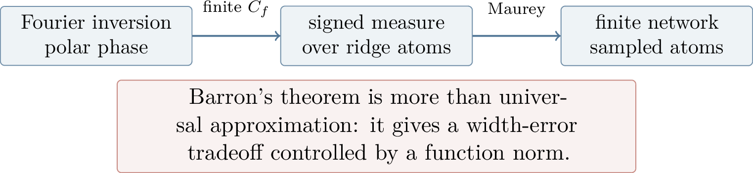
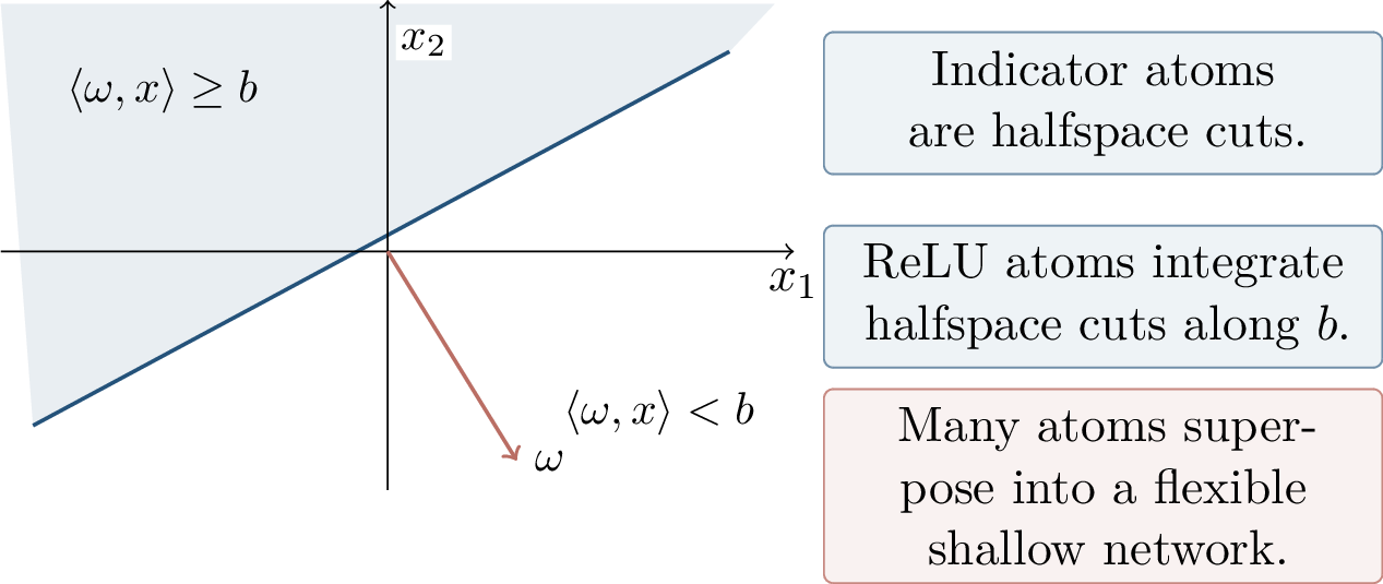
The passage from indicator atoms to ReLU atoms is conceptually simple. In one dimension, \[\require{physics} (t)_+ = \int_0^\infty \mathbf{1}\{t\ge b\}\,\dd b.\] On a bounded domain this integral only needs thresholds in a bounded interval. Thus a ReLU ridge function is an accumulated family of halfspace cuts. This is why it is natural for the Fourier argument to produce threshold atoms first and for the final approximation theorem to be stated using standard neural network activations.
Representation Versus Approximation The signed integral is an exact infinite-width representation. The finite network obtained later is only an approximation, because it replaces the full measure by finitely many atoms. The size of the measure controls how many atoms are needed.
1.1.14.2 A Gaussian Example
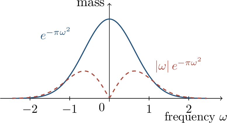
The Gaussian illustrates why Barron complexity is not simply a disguised dimension count. Under the Fourier convention used here, \[f(x)=\exp(-\pi\left\lVert x \right\rVert^2) \qquad\Longrightarrow\qquad \widehat f(\omega)=\exp(-\pi\left\lVert \omega \right\rVert^2).\] Therefore \[\require{physics} \begin{align} C_f &= 2\pi\int_{\R^d}\left\lVert \omega \right\rVert e^{-\pi\left\lVert \omega \right\rVert^2}\,\dd\omega \\ &\le 2\pi \left( \int_{\R^d}\left\lVert \omega \right\rVert^2 e^{-\pi\left\lVert \omega \right\rVert^2}\,\dd\omega \right)^{1/2} = O(\sqrt d). \end{align}\] Here the last equality follows from the fact that \(e^{-\pi\left\lVert \omega \right\rVert^2}\) factorizes over coordinates and has total integral one. In one coordinate, \[\require{physics} \int_{\R}\omega^2 e^{-\pi\omega^2}\,\dd\omega=\frac{1}{2\pi},\] so by additivity of second moments, \[\require{physics} \int_{\R^d}\left\lVert \omega \right\rVert^2 e^{-\pi\left\lVert \omega \right\rVert^2}\,\dd\omega = \frac{d}{2\pi}.\] Consequently \(C_f\le \sqrt{2\pi d}\). This calculation is elementary, but it captures a central lesson: a radial Gaussian in \(d\) dimensions does not pay a grid cost \(c^d\) in the Barron norm; it pays the typical Euclidean radius of its Fourier mass.
The reference notes emphasize the same point probabilistically: the Gaussian Fourier density has coordinate variance of constant order, so the expected Euclidean norm scales like \(\sqrt d\), not exponentially in \(d\).
This example should not be confused with kernel density estimation. In KDE one starts from samples and smooths the empirical distribution: \[\widehat p_h(x)=\frac{1}{n}\sum_{i=1}^n K_h(x-X_i).\] Rates for nonparametric estimation often degrade with dimension through volume effects. Barron approximation is a different statement: given a target function with a controlled representation, a shallow network can approximate it at a rate governed by \(C_f\). The theorem is about approximation from a function representation, not about automatically estimating an arbitrary high-dimensional distribution from few samples. The reference notes also point out that \(C_f\) behaves naturally under operations such as addition and dilation, so it is a genuine complexity measure rather than a one-off calculation.
This distinction between approximation and estimation is worth stressing. In approximation theory, the target function is fixed and the question is how large a model class must be to represent it well. In statistical estimation, the learner sees only samples and must choose a function from data. A small Barron norm can make the approximation part favorable, but one still needs separate arguments for sample complexity and optimization. Later chapters will revisit exactly this separation.
1.1.15 Sparsification: From Mixtures to Finite Networks↩︎
The Barron representation places the target in a scaled convex hull of simple atoms. Let \[S=\{v_{w,b}: v_{w,b}(x)=\sigma(\left\langle w,x \right\rangle+b)\}\] or a related dictionary of indicator atoms. Abstractly, the representation says \[f-f(0)\in A\,\operatorname{conv}(\pm S), \qquad A\lesssim C_f.\] Approximation now becomes geometry in a Hilbert space: how well can a point in a convex hull be approximated by an average of few atoms?
This reformulation is powerful because it removes most of the neural-network syntax. The atoms may be ridge functions, threshold functions, or signed versions of them, but the finite-width theorem only needs two facts: the target lies in a scaled convex hull, and the atoms have bounded norm in the space where the approximation error is measured. For example, when the error is \(L^2(\mu)\) on a probability distribution \(\mu\), the Hilbert norm is \[\require{physics} \left\lVert h \right\rVert_{L^2(\mu)} = \left(\int \left\lvert h(x) \right\rvert^2\,\dd\mu(x)\right)^{1/2}.\] On a bounded domain, common ridge atoms have bounded \(L^2(\mu)\) norm, so the abstract lemma below applies directly.
Lemma 1.2 (Maurey sparsification). Let \(X\in\operatorname{conv}(S)\) in a Hilbert space, and suppose \(\left\lVert v \right\rVert\le R\) for all \(v\in S\). Then for every \(m\ge1\) there exist \(v_1,\dots,v_m\in S\) such that \[\left\|X-\frac{1}{m}\sum_{j=1}^m v_j\right\|^2 \le \frac{R^2}{m}.\]
Proof. Since \(X\in\operatorname{conv}(S)\), write \(X=\E[V]\) for a random atom \(V\in S\). Draw independent copies \(V_1,\dots,V_m\). Then \[\begin{align} \E\left\|X-\frac{1}{m}\sum_{j=1}^m V_j\right\|^2 &= \frac{1}{m}\,\E\left\lVert V-X \right\rVert^2 \\ &= \frac{1}{m}\,\bigl(\E\left\lVert V \right\rVert^2-\left\lVert X \right\rVert^2\bigr) \le \frac{R^2}{m}. \end{align}\] Since the expected squared error is at most \(R^2/m\), at least one sampled average has error no larger than this. This sampled average is a sparse convex combination, hence a finite network. ◻
Maurey’s lemma explains the \(m^{-1/2}\) error rate: squared error scales like \(1/m\), so norm error scales like \(1/\sqrt m\). It is the sampling heart of Barron’s finite-width theorem.
Notice the role of independence in the proof. When the \(V_j\) are sampled independently from a distribution whose mean is \(X\), the cross terms cancel after taking expectation. What remains is the variance of one atom divided by \(m\). This is the same variance-reduction mechanism behind Monte Carlo averaging, but here it is used as an existence argument: a random construction with small expected error implies that at least one deterministic collection of atoms has small error.
The Meaning of the Rate Maurey’s lemma gives \(\left\lVert X-m^{-1}\sum_j v_j \right\rVert=O(m^{-1/2})\). In squared \(L^2\) error this is \(O(1/m)\). Barron approximation rates are often stated in one of these two equivalent forms, so it is important to check whether the quantity being bounded is the norm or the squared norm.
1.1.15.1 Frank-Wolfe as Constructive Sparsification
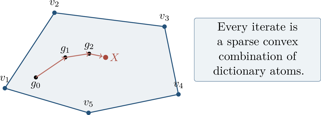
The reference notes also describe a deterministic, greedy view. Suppose the current approximation has the form \[g_{i-1}=\sum_{j=1}^{i-1}\alpha_j v_j,\] and at step \(i\) we solve \[\min_{\lambda\in[0,1],\,v_i\in S} \left\| \lambda g_{i-1}+(1-\lambda)v_i-X \right\|^2.\] Equivalently, \[g_i=\lambda g_{i-1}+(1-\lambda)v_i\] is a new sparse convex combination with one additional atom. This is the Frank-Wolfe viewpoint: move inside the convex hull by adding a vertex that most improves the objective.
The geometric picture is that \(X\) is a point in a large convex body and the dictionary atoms are its extreme or candidate vertices. The greedy method keeps the iterate inside the convex body while increasing the number of active vertices by one. The step size \(\lambda\) balances two goals: preserve the useful part of the current approximation and move toward a newly selected atom that decreases the residual.
Lemma 1.3 (Greedy approximation rate). Assume \(X\in\operatorname{conv}(S)\) and \(\left\lVert v \right\rVert\le R\) for all \(v\in S\). If each step chooses the best point of the form \[g_i=\lambda g_{i-1}+(1-\lambda)v_i, \qquad \lambda\in[0,1],\quad v_i\in S,\] then \[\left\lVert g_i-X \right\rVert^2\le \frac{R^2}{i}.\]
Proof. As in Maurey’s lemma, write \(X=\E[V]\) for a random atom \(V\in S\). Because the greedy step is at least as good as choosing a random atom, for any \(\lambda\in[0,1]\), \[\begin{align} \left\lVert g_i-X \right\rVert^2 &\le \E\left\lVert \lambda(g_{i-1}-X)+(1-\lambda)(V-X) \right\rVert^2\\ &= \lambda^2\left\lVert g_{i-1}-X \right\rVert^2 +(1-\lambda)^2\E\left\lVert V-X \right\rVert^2 . \end{align}\] The cross term vanishes since \(\E[V-X]=0\). Using \(\E\left\lVert V-X \right\rVert^2\le R^2\) and choosing \(\lambda=1-1/i\), an induction gives \(\left\lVert g_i-X \right\rVert^2\le R^2/i\). ◻
This deterministic lemma explains the same rate as Maurey’s sampling argument. It also exposes the algorithmic caveat. The best atom search over \(S\) can itself be a hard nonconvex problem. Thus the Barron theorem plus sparsification proves that a good finite representation exists, but it does not prove that stochastic gradient descent, initialized in parameter space, will find that representation. Approximation, statistics, and optimization are related but distinct questions.
In other words, Frank-Wolfe gives a constructive proof only relative to an oracle for the best atom. If the dictionary is finite and small, this oracle may be implemented by search. For neural-network dictionaries, the atom usually contains continuous parameters such as \(w\) and \(b\), so the oracle is itself an optimization problem. The chapter therefore deliberately stops short of claiming a practical training algorithm from the Barron proof alone.
1.1.16 Depth Separation↩︎
The second theme of the chapter asks a different expressivity question. Can a deep network represent some functions exponentially more efficiently than a shallower one? The aim is to construct a target with a compact deep representation and then show that shallower networks require many more units to approximate it. The cleanest mechanism in this chapter is one-dimensional and geometric: repeated composition creates many oscillations, and shallow piecewise-linear functions cannot track all of them.
Depth separation results should be read as lower bounds against a competing architecture class. They do not merely show that a deep network can represent an oscillatory function; that part is the easy construction. They also show that networks with restricted depth and controlled size cannot approximate the same function well. Telgarsky’s sawtooth construction [6] is particularly transparent because both sides of the comparison can be studied using elementary piecewise-affine geometry. Other depth separations, such as the radial construction of Eldan and Shamir [5], use different analytic mechanisms, but the conceptual message is similar: depth can encode repeated structure compactly.
1.1.16.1 The Tent Map Gadget
Definition 1.6 (Tent map). Define \(m:\R\to\R\) by \[m(x)= \begin{cases} 2x, & 0\le x\le \frac{1}{2},\\ 2-2x, & \frac{1}{2}<x\le 1,\\ 0, & \text{otherwise}. \end{cases}\]
![Figure 27: The tent map m. Its graph is a single triangle on [0,1] and zero outside.](/article/2607.01311/ms-figure31.png "fig:")
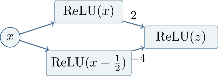
The tent map has a constant-size ReLU implementation. Let \[z(x)=2\relu(x)-4\relu\!\left(x-\frac{1}{2}\right).\] Then \[m(x)=\relu(z(x)).\] Indeed, on \([0,1/2]\) this is \(2x\); on \((1/2,1]\) it is \(2-2x\); and outside the interval the final ReLU clips the negative part to zero.
The point of writing \(m\) as a small ReLU module is that the same module can be reused. On each copy, the input and output both lie in \([0,1]\) when the input starts in \([0,1]\). Therefore the output of one tent module is a valid input to the next. This closure property is what makes repeated composition a natural operation for a deep network.
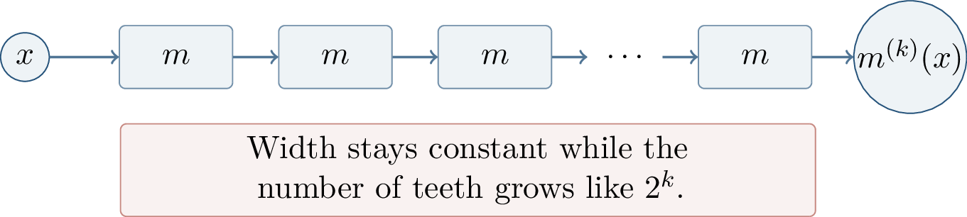
The key phenomenon appears when we compose \(m\) with itself. Write \[m^{(k)} = \underbrace{m\circ m\circ\cdots\circ m}_{k\text{ times}}.\] Each iteration doubles the number of teeth on \([0,1]\). Thus \(m^{(k)}\) has \(2^k\) teeth, while a network implementing it is obtained by stacking \(k\) copies of the same constant-size module.
This is the simplest possible example of compositional efficiency. A shallow network must create many breakpoints in one layer hierarchy, while the deep network creates them by reusing a fixed transformation. The number of parameters grows only linearly with the number of compositions, whereas the number of affine pieces grows exponentially.
![Figure 29: Composition creates teeth. The first, second, and third iterates have one, two, and four teeth on [0,1].](/article/2607.01311/ms-figure33.png "fig:")
1.1.16.2 Sawtooth Complexity
Definition 1.7 (\(t\)-sawtooth function). A univariate function \(f:\R\to\R\) is \(t\)-sawtooth if its domain can be partitioned into at most \(t\) intervals on each of which \(f\) is affine.
The tent map \(m\) is \(4\)-sawtooth when the two outside flat pieces are included. On the interval \([0,1]\), \(m^{(k)}\) has \(2^k\) teeth. The following elementary rules are the counting engine behind the lower bound.
The definition deliberately counts affine pieces rather than neurons. For univariate ReLU networks, affine pieces are a convenient proxy for expressive complexity: if two functions differ on many alternating small intervals, then an approximator with too few affine pieces cannot follow the alternation. Sawtooth counting is therefore a bridge from network architecture to an integral approximation lower bound.
Lemma 1.4 (Calculus of sawtooth functions). If \(f\) is \(s\)-sawtooth and \(g\) is \(t\)-sawtooth, then \[af+b \text{ is } s\text{-sawtooth}, \qquad f+g \text{ is } (s+t)\text{-sawtooth},\] and \[f\circ g \text{ is at most } st\text{-sawtooth}.\]
Proof. Affine rescaling does not create new breakpoints. The sum \(f+g\) can change formula only at a breakpoint of either function, so the partitions may be refined to at most \(s+t\) intervals. For the composition, each affine piece of \(g\) maps an interval into an interval on the input line of \(f\); this image can cross at most \(s\) pieces of \(f\). Across \(t\) pieces of \(g\), this gives at most \(st\) affine pieces. ◻
Corollary 1.1 (Shallow ReLU sawtooth bound). For a univariate ReLU network of depth \(L\) with at most \(2^L\) hidden units, the output has sawtooth complexity at most \(2^{O(L^2)}\).
Proof idea. A ReLU gate is piecewise affine. Within a layer, summing units adds breakpoints at most additively. Passing through the next layer composes piecewise-affine maps, and composition multiplies the number of pieces. With depth \(L\) and at most \(2^L\) hidden units total, the repeated additive and multiplicative growth is bounded by \(2^{O(L^2)}\). ◻
The exact constant hidden in \(O(L^2)\) is not important for the qualitative separation. What matters is the comparison with the target \(m^{(L^2+2)}\), whose number of teeth is of order \(2^{L^2}\) at a scale carefully chosen so that the lower-bound counting argument leaves a constant amount of \(L^1\) error. This is a common pattern in expressivity lower bounds: the target is tuned so that the upper bound for the deep class and the lower bound for the shallow class meet at sharply separated scales.
1.1.16.3 Telgarsky’s Separation
Theorem 1.4 (Telgarsky depth separation). For every sufficiently large \(L\), there exists a function \(f:[0,1]\to[0,1]\) computed by a ReLU network with depth \(O(L^2)\) and \(O(L^2)\) units such that every ReLU network \(g\) with depth at most \(L\) and at most \(2^L\) units satisfies \[\require{physics} \int_0^1 \left\lvert f(x)-g(x) \right\rvert\,\dd x \ge \frac{1}{32}.\] One concrete target is \[f=m^{(L^2+2)}.\]
The deep implementation is short because it reuses the same module many times. After \(k\) modules, the width is still constant, while the number of teeth is \(2^k\). This is the essence of the separation: composition is natural for deep networks and expensive for shallow networks.
The theorem should be interpreted as a comparison at fixed approximation accuracy. The deep network computes the target exactly by construction. A shallower network is allowed exponentially many units in \(L\), but its sawtooth complexity is still too small to align with the alternating peaks and valleys of \(m^{(L^2+2)}\). The lower bound is therefore not a parameter-count statement alone; it is a statement about how those parameters are organized across layers.
The proof picture is the following. The target \(f=m^{(L^2+2)}\) has roughly \(2^{L^2+2}\) small triangles. A shallow network \(g\), because it has only limited sawtooth complexity, has long affine pieces at the relevant scale. On such an affine piece, \(g\) cannot follow both the rising and falling sides of many target triangles. A constant fraction of those triangles are missed.
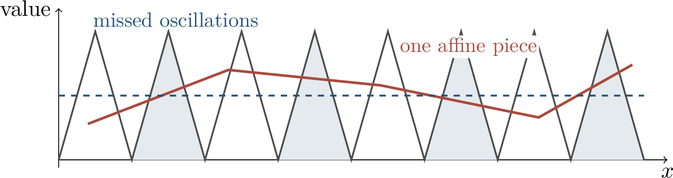
The area calculation is explicit. The function \(m^{(L^2+2)}\) has about \(2^{L^2+2}\) triangles on \([0,1]\), and each triangle has area \[\frac{1}{2}\cdot\frac{1}{2}\cdot 2^{-(L^2+2)} = 2^{-L^2-4}.\] The reference notes phrase the lower bound as follows: after accounting for the triangles that can be handled near boundaries of the affine pieces, at least a constant fraction of the remaining triangles are missed. This gives \[\require{physics} \int_0^1\left\lvert f(x)-g(x) \right\rvert\,\dd x \ge \frac{1}{2}\bigl(2^{L^2+2}-1-2\cdot2^{L^2}\bigr) 2^{-L^2-4} \ge \frac{1}{32}.\]
The constants in this calculation are less important than the counting mechanism. A shallow approximator can place breakpoints at some of the triangle boundaries, but it cannot place them at enough boundaries. On many triangles it must behave essentially affinely across a region where the target goes up and then down. Such a function must miss a definite amount of area on at least one side of the triangle. Summing these small missed areas over a constant fraction of the triangles gives a constant total \(L^1\) error.
The theorem proves that depth can be exponentially more efficient than width for some explicit functions. It does not say that every practical task has this structure, and it does not prove that training will discover the compact deep representation. It is an approximation lower bound, not an optimization theorem. Its value is conceptual: composition can create structure that is unnatural for shallow piecewise-linear approximators.
Several other separation results point in the same broad direction. Bengio and Delalleau studied separations through sum-product style architectures. Eldan and Shamir proved that depth three can beat depth two using radial functions and Fourier analysis [5]. Telgarsky’s result gives an explicit ReLU sawtooth construction with an \(L^1\) lower bound [6]. Lee, Ge, Ma, Risteski, and Arora developed deeper analogues of Barron-type expressivity [26]. The reference notes also mention a circuit-complexity analogy: constant-depth threshold circuits show enormous gaps between what counting arguments prove exists and what explicit constructions can currently separate.
Depth Separation Is Not the Whole Story Depth separation explains why some functions are compactly compositional. It does not say that a particular data distribution has such a target, that the compact network is statistically identifiable, or that gradient descent will recover it. These are the next questions after expressivity.
1.1.17 From Expressivity to Optimization↩︎
Approximation and separation results answer the question “does a good network exist?” Training asks a different question. Given data \((x_i,y_i)_{i=1}^n\), we choose parameters \(W\), such as \[W=(W_1,b_1,\dots,W_L,b_L),\] by empirical risk minimization: \[\min_W \widehat R(W) = \min_W \sum_{i=1}^n \ell\!\left(f(x_i;W),y_i\right).\] For squared loss, \[\ell(\widehat y,y)=\frac{1}{2}\left\lVert \widehat y-y \right\rVert^2.\]
Neural-network optimization is hard because the empirical risk is typically nonconvex, has many equivalent parameterizations, contains valleys and saddles, and depends on the finite sample. The classical convex theory is therefore not a complete explanation of deep learning, but it is the right baseline. It teaches us which curvature assumptions make gradient descent provably reliable.
This baseline is useful for two reasons. First, it gives a vocabulary: smoothness controls how quickly gradients change, strong convexity controls how sharply the objective grows away from the minimizer, and the ratio \(B/\alpha\) acts as a condition number. Second, it provides a contrast with neural networks. In a nonconvex network objective, the same update rule \(W_{t+1}=W_t-\eta\nabla\widehat R(W_t)\) is used, but the global geometry no longer guarantees that every descent direction points toward a unique optimum. Later theories of overparameterization, lazy training, and implicit bias can be viewed as attempts to recover some useful part of the convex story in a nonconvex parameterization.
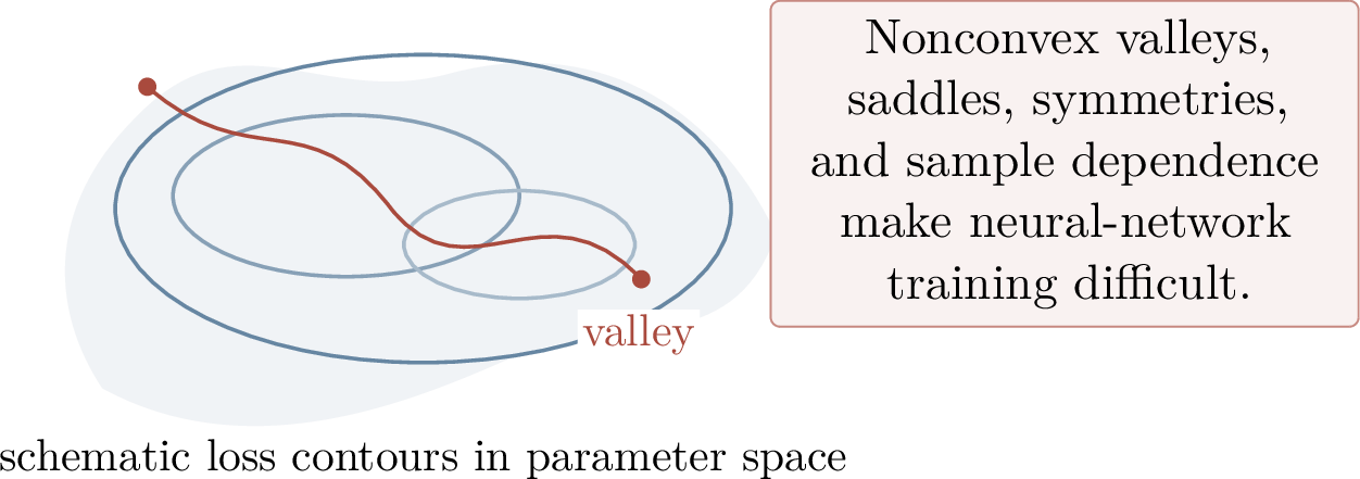
1.1.17.1 Convex Functions and Gradient Descent
Definition 1.8 (Convex function). A differentiable function \(F:\R^p\to\R\) is convex if for all \(x,y\in\R^p\) and all \(\lambda\in[0,1]\), \[F(\lambda x+(1-\lambda)y) \le \lambda F(x)+(1-\lambda)F(y).\]
For a convex function, every sublevel set \[\{x:F(x)\le c\}\] is convex. Gradient descent uses the update \[x_{t+1}=x_t-\eta\nabla F(x_t),\] where \(\eta>0\) is the stepsize. Geometrically, the negative gradient points inward across the boundary of a sublevel set; analytically, it is the direction of steepest local decrease.
The first-order characterization of differentiable convex functions is \[F(y)\ge F(x)+\left\langle \nabla F(x),y-x \right\rangle.\] Thus the tangent hyperplane at \(x\) is a global lower bound. This property is the main reason convex optimization is tractable: local derivative information contains global information. Neural-network objectives generally lack this property, so a small gradient need not certify global optimality.
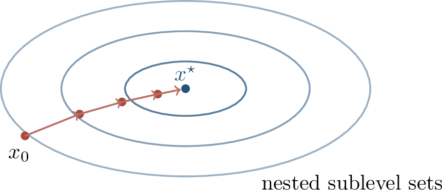
Definition 1.9 (\(B\)-smoothness). A differentiable function \(F\) is \(B\)-smooth if \[\left\lVert \nabla F(x)-\nabla F(y) \right\rVert \le B\left\lVert x-y \right\rVert\] for all \(x,y\). If \(F\) is twice differentiable, this is equivalent to \[\nabla^2F(x)\preceq B I\] for all \(x\).
Smoothness says that the gradient cannot change too abruptly. Therefore a local linear approximation remains useful over a controlled distance, which is why a properly chosen gradient step does not overshoot.
Equivalently, \(B\)-smoothness gives the descent lemma \[F(y) \le F(x)+\left\langle \nabla F(x),y-x \right\rangle +\frac{B}{2}\left\lVert y-x \right\rVert^2 .\] Substituting \(y=x-\eta\nabla F(x)\) shows why stepsizes of order \(1/B\) are natural: the linear decrease from moving against the gradient must dominate the quadratic error term.
Definition 1.10 (\(\alpha\)-strong convexity). A differentiable function \(F\) is \(\alpha\)-strongly convex if \[F(y)\ge F(x)+\left\langle \nabla F(x),y-x \right\rangle +\frac{\alpha}{2}\left\lVert y-x \right\rVert^2\] for all \(x,y\). If \(F\) is twice differentiable, this is equivalent to \[\nabla^2F(x)\succeq \alpha I\] for all \(x\).
Strong convexity says that the function grows at least quadratically away from the minimizer. In particular, the minimizer is unique. The reference notes motivate the condition by saying that if a quadratic lower model fits under the local linear approximation, then the optimum cannot be too far away.
When \(F\) is both \(B\)-smooth and \(\alpha\)-strongly convex, the Hessian eigenvalues, in the twice differentiable case, lie between \(\alpha\) and \(B\). The condition number \(\kappa=B/\alpha\) measures how elongated the level sets can be. A large \(\kappa\) means that gradient descent may make slow progress along flat directions even though the function is still convex.
Theorem 1.5 (Classical gradient-descent guarantee). Let \(F:\R^p\to\R\) be \(B\)-smooth and \(\alpha\)-strongly convex, and let \(x^\star\) be its unique minimizer. If gradient descent uses \[\eta=\frac{1}{B},\] then \[\left\lVert x_{t+1}-x^\star \right\rVert^2 \le \left(1-\frac{\alpha}{B}\right)\left\lVert x_t-x^\star \right\rVert^2.\] Consequently, the function error also decreases geometrically: \[F(x_t)-F(x^\star) \le \left(1-\frac{\alpha}{B}\right)^t \bigl(F(x_0)-F(x^\star)\bigr)\]
Proof sketch. The smoothness inequality with \(y=x_t-\frac{1}{B}\nabla F(x_t)\) gives \[F(x_{t+1}) \le F(x_t)-\frac{1}{2B}\left\lVert \nabla F(x_t) \right\rVert^2 .\] Strong convexity implies the Polyak-Lojasiewicz-type bound \[\frac{1}{2}\left\lVert \nabla F(x_t) \right\rVert^2 \ge \alpha\bigl(F(x_t)-F(x^\star)\bigr),\] which follows by minimizing the quadratic lower bound from strong convexity. Combining the two inequalities yields \[F(x_{t+1})-F(x^\star) \le \left(1-\frac{\alpha}{B}\right) \bigl(F(x_t)-F(x^\star)\bigr),\] and iteration gives the stated function-value convergence.
For the distance contraction, one uses the standard interpolation inequality for \(B\)-smooth and \(\alpha\)-strongly convex functions, \[\begin{align} \left\langle \nabla F(x)-\nabla F(y),x-y \right\rangle &\ge \frac{\alpha B}{\alpha+B}\left\lVert x-y \right\rVert^2 +\frac{1}{\alpha+B} \left\lVert \nabla F(x)-\nabla F(y) \right\rVert^2 . \end{align}\] Apply this with \(y=x^\star\), where \(\nabla F(x^\star)=0\), and expand \[\left\|x_t-\frac{1}{B}\nabla F(x_t)-x^\star\right\|^2 .\] The gradient-square term has a nonpositive coefficient, and the remaining coefficient is at most \(1-\alpha/B\). This gives the displayed contraction of squared distance. In the twice differentiable quadratic case, the same argument reduces to the elementary fact that the eigenvalues of \(I-\frac{1}{B}\nabla^2 F\) lie in \([0,1-\alpha/B]\). ◻
This theorem is the clean convex world: one basin, one minimizer, curvature bounded above and below, and gradients that reliably point toward the optimum. Neural networks are not generally in this regime. However, later chapters will study overparameterized settings, including neural tangent kernel regimes, where the local geometry of training can behave like a controlled kernel method even though the parameterized objective is nonconvex [8]–[10].
1.1.18 Limitations and the Road Ahead↩︎
The chapter’s main conclusions can be summarized as follows. Barron theory identifies a spectral function class for which shallow networks have dimension-friendly approximation rates. Maurey’s lemma and Frank-Wolfe sparsification explain why an infinite signed mixture can be compressed into a finite network. Depth separation shows that repeated composition can create functions that shallow networks approximate only at exponential cost. Finally, optimization theory reminds us that the existence of a representation does not guarantee that a training algorithm will find it.
These conclusions should be understood as complementary rather than competing. Barron theory gives a positive result for shallow networks under a spectral regularity condition. Depth separation gives a negative result for shallow networks on a specially constructed compositional target. Convex optimization gives a positive algorithmic result under curvature assumptions that neural networks usually do not satisfy globally. Together they define the agenda for the next part of the monograph: identify structural assumptions under which approximation, generalization, and optimization can all be controlled at the same time.
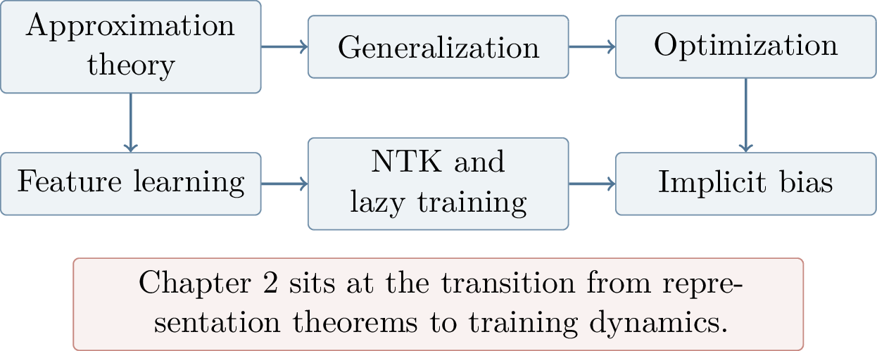
Barron bounds are strongest for functions with small spectral first moment. Telgarsky’s construction is explicit and instructive, but it is a stylized one-dimensional target rather than a model of all practical data. The main open questions are therefore structural and algorithmic: which natural high-dimensional tasks have small Barron or compositional norms, which depth separations correspond to realistic architectures and distributions, and when does overparameterized optimization behave enough like convex optimization to be analyzable?
Chapter Synthesis This chapter develops three lessons. First, Fourier first-moment control places a function in a Barron-type convex hull of ridge atoms. Second, Maurey’s lemma and Frank-Wolfe sparsification turn convex-hull membership into finite-width approximation rates. Third, depth can be exponentially more efficient than shallowness for compositional functions, but expressivity alone does not solve the training problem.
For the Barron approximation viewpoint, see Barron’s original theorem on superpositions of sigmoidal functions [4]. For depth separation, see Telgarsky’s sawtooth construction [6] and the radial construction of Eldan and Shamir [5]; Yarotsky’s approximation results provide a related quantitative ReLU perspective [7]. For optimization background and the convex baseline used here, see standard learning-theory and optimization treatments such as [2]. Later chapters connect this baseline to overparameterized neural-network training [8]–[10].
2 Optimization, Kernels, and Implicit Bias↩︎
2.0.1 From Optimization to the NTK↩︎
The previous chapter separated approximation and expressivity from optimization. This chapter begins the optimization side of the story. In convex problems, gradients reliably lead to a unique global solution under appropriate curvature assumptions. In deep learning, however, the empirical risk is nonconvex, the model is highly overparameterized, and many very different parameter vectors may fit the same training data. The neural tangent kernel (NTK) gives one mathematically clean regime in which gradient descent on a huge nonconvex network behaves like a kernel method.
The central idea is to stop looking only at the parameters and instead track the vector of predictions on the training sample. A parameter vector \(w\in\R^p\) may be very high-dimensional and the loss surface in \(w\)-space may be nonconvex. But the training predictions form a finite vector in \(\R^N\). When the network is sufficiently wide, the map from parameters to this prediction vector can remain close to its first-order Taylor expansion near initialization. In that regime, the complicated nonlinear optimization problem reduces, along the training set, to a linear least-squares dynamics with a kernel matrix determined by parameter gradients.
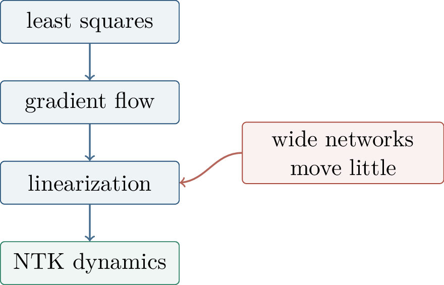
The guiding question is: \[\textit{Why can gradient descent fit training data in a huge nonconvex neural network?}\] The answer developed here is not the whole answer for practical deep learning. Rather, it is a controlled theorem in a particular limit: when the network is wide enough and properly scaled, the parameters move only a little, so the network remains close to its tangent approximation at initialization. In that lazy-training regime, training can be described through a kernel matrix on the training examples.
Historically, this viewpoint is associated with the neural tangent kernel of Jacot, Gabriel, and Hongler [8], and with subsequent overparameterized convergence analyses such as [9], [10]. These works do not claim that all useful neural networks are lazy kernel machines. Rather, they identify a precise mathematical regime in which a highly nonconvex parameterization has a provably stable tangent kernel and therefore trainable finite-sample dynamics.
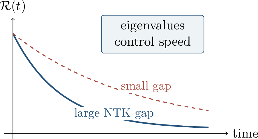
2.0.1.1 Finite-Sample Setup
Fix a training set \(\{(x_i,y_i)\}_{i=1}^N\) and parameters \(w\in\R^p\). It is convenient to suppress the input points and collect the network predictions into a vector \[f(w)= \begin{bmatrix} f(x_1;w)\\ \vdots\\ f(x_N;w) \end{bmatrix}, \qquad y= \begin{bmatrix} y_1\\ \vdots\\ y_N \end{bmatrix}.\] The chapter uses a positive output scale \(\alpha>0\), so the prediction vector is \[z(w)=\alpha f(w),\] and the square loss on the training set is \[\mathcal{R}(z) = \frac{1}{2}\left\lVert z-y \right\rVert_2^2 = \frac{1}{2}\left\lVert \alpha f(w)-y \right\rVert_2^2.\] One should think of increasing \(\alpha\) as part of the wide-network scaling: small parameter motion can still produce meaningful prediction motion.
The notation separates two spaces. The parameter \(w\) lives in \(\R^p\), where \(p\) may be much larger than \(N\). The vector \(z(w)\) lives in \(\R^N\), one coordinate per training example. The loss \(\mathcal{R}(z)=\frac{1}{2}\left\lVert z-y \right\rVert^2\) is convex as a function of \(z\), but generally nonconvex as a function of \(w\) because \(z=z(w)\) is nonlinear. NTK analysis asks whether, along the actual gradient-flow path, the induced dynamics in \(z\)-space remain close to the convex linear dynamics.
The training-set Jacobian is \[J(w)= \begin{bmatrix} \grad_w f(x_1;w)^\top\\ \vdots\\ \grad_w f(x_N;w)^\top \end{bmatrix}\in\R^{N\times p}.\] Later, along a training trajectory \(w(t)\), we write \(J_t=J(w(t))\). The matrix \(J_t\) maps a parameter perturbation to the first-order change in all training predictions.
This Jacobian is the finite-sample analogue of a feature map. Its \(i\)-th row is the tangent feature vector of the example \(x_i\): \[\phi_w(x_i)=\grad_w f(x_i;w)\in\R^p.\] Two examples are similar in the tangent sense if their tangent feature vectors have a large inner product. The empirical NTK introduced below is exactly the Gram matrix of these tangent features.
Prediction-Space Viewpoint The loss is a simple quadratic in the prediction vector \(z\). The difficulty is that \(z\) is generated by a nonlinear map \(w\mapsto \alpha f(w)\). NTK theory studies a regime in which this nonlinear map behaves nearly like its linearization on the training trajectory.
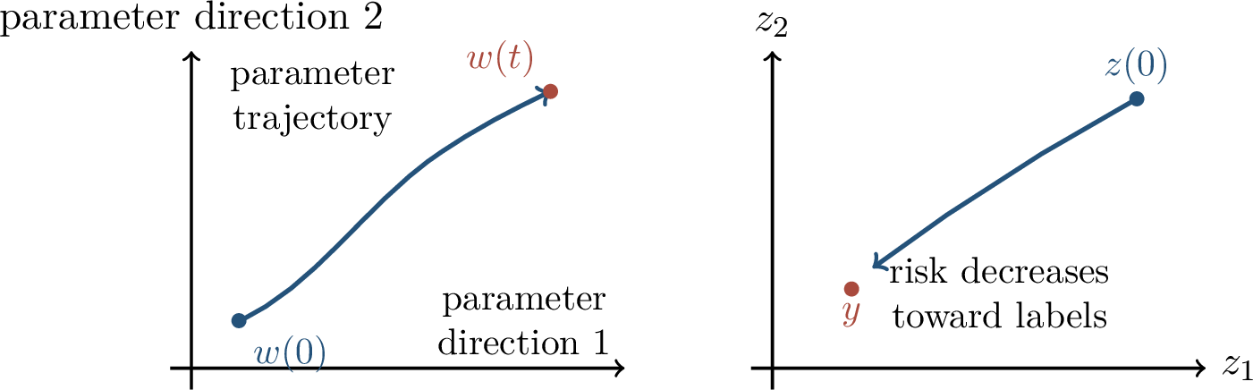
2.0.2 Least Squares and Gradient Flow↩︎
Before neural networks, we analyze the model problem \[\min_x F(x)=\frac{1}{2}\left\lVert Ax-b \right\rVert_2^2, \qquad A\in\R^{N\times p},\quad b\in\R^N.\] The gradient and Hessian are \[\grad F(x)=A^\top(Ax-b), \qquad \grad^2F(x)=A^\top A.\] If \(A^\top A\succ0\), then \(F\) is strongly convex and has a unique minimizer. This is the clean convex case from the previous chapter. If \(A^\top A\) is singular, there may be many minimizers in parameter space, but the residual dynamics are still governed by the output-space matrix \(AA^\top\). This distinction is important for neural networks: parameters may be highly redundant while the predictions on the training set can still be controlled by a well-conditioned Gram matrix.
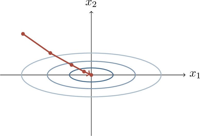
2.0.2.1 Residual Dynamics
Let \[r_t=Ax_t-b.\] Gradient descent with stepsize \(\eta\) gives \[x_{t+1}=x_t-\eta A^\top r_t.\] Multiplying by \(A\) converts the parameter update into a residual update: \[r_{t+1} = Ax_{t+1}-b = r_t-\eta AA^\top r_t.\] Thus the matrix that controls training in residual space is \(AA^\top\), the Gram matrix of the rows of \(A\).
This calculation contains the algebraic skeleton of the NTK proof. The parameter update involves \(A^\top r_t\), but the residual update involves \(AA^\top r_t\). Hence convergence depends not directly on the number of parameters \(p\), but on whether the rows of \(A\), viewed as features of the training examples, span all residual directions in \(\R^N\). If \(AA^\top\) has a small eigenvalue, the corresponding residual component decays slowly; if \(AA^\top\) is singular, some residual direction cannot be corrected by the model.
The gradient-flow limit for least squares satisfies \[\dot{r}(t)=-AA^\top r(t), \qquad r(t)=\exp(-AA^\top t)r(0).\] If \(AA^\top\succ0\), then \(\left\lVert r(t) \right\rVert_2\) decays exponentially.
Proof. The gradient-flow equation is \[\dot{x}(t)=-A^\top(Ax(t)-b)=-A^\top r(t).\] Differentiating \(r(t)=Ax(t)-b\) gives \[\dot{r}(t)=A\dot{x}(t)=-AA^\top r(t).\] Solving this linear ODE yields the matrix-exponential formula. If \(\lambda_{\min}(AA^\top)>0\), then each eigencomponent decays at rate at least \(\lambda_{\min}(AA^\top)\). ◻
To see the eigencomponent statement explicitly, write \[AA^\top=Q\Lambda Q^\top, \qquad \Lambda=\diag(\lambda_1,\dots,\lambda_N).\] In the coordinates \(\widetilde{r}(t)=Q^\top r(t)\), \[\dot{\widetilde{r}}_i(t)=-\lambda_i\widetilde{r}_i(t), \qquad \widetilde{r}_i(t)=e^{-\lambda_i t}\widetilde{r}_i(0).\] The smallest positive eigenvalue controls the slowest learnable direction. This is why NTK proofs focus so much attention on lower bounding the minimum eigenvalue of the empirical tangent kernel.
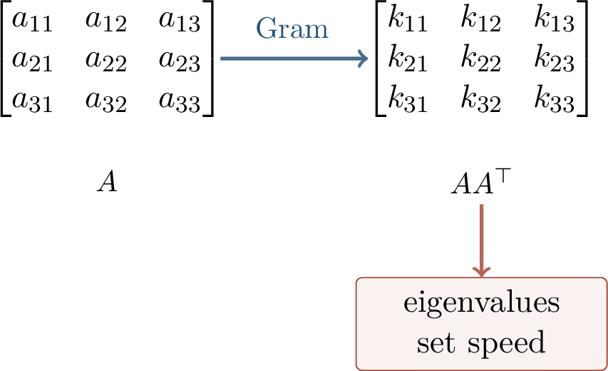
This warm-up matters because the same algebra reappears with \[A \quad\longleftrightarrow\quad J(w(0)).\] The linearized neural network is a least-squares problem whose feature matrix is the Jacobian at initialization.
The Warm-Up in One Line Least squares has residual flow \(\dot{r}=-AA^\top r\). Linearized neural networks have the same form with \(A\) replaced by the training-set Jacobian \(J_0\). The NTK is therefore the neural-network version of a least-squares Gram matrix.
2.0.2.2 GD, SGD, Acceleration, and Flow
The reference notes review several descent viewpoints. For a risk \(\mathcal{R}(w)\), full gradient descent, stochastic gradient descent, accelerated gradient descent, and gradient flow may be written schematically as \[\begin{align} \text{GD:}\quad &w_{t+1}=w_t-\eta\grad\mathcal{R}(w_t),\\ \text{SGD:}\quad &w_{t+1}=w_t-\eta\grad_w\ell_i(w_t),\\ \text{AGD:}\quad &x_{t+1}=y_{t+1}+\mu(y_{t+1}-y_t),\\ \text{Flow:}\quad &\dot{w}(t)=-\grad\mathcal{R}(w(t)). \end{align}\] SGD uses a noisy gradient estimate from one example or a minibatch. Acceleration uses information from past gradients, often improving iteration complexity in convex problems. Gradient flow is the continuous-time limit obtained as the stepsize tends to zero; it removes discretization details and reveals the ODE structure that NTK proofs exploit.
Continuous time should not be mistaken for a different algorithmic principle. It is a mathematical idealization of small-step gradient descent. The benefit is that risk decay can be derived by differentiating \(\mathcal{R}(w(t))\) and using matrix inequalities. Discrete-time results require extra stepsize conditions, but the same spectral quantities appear.
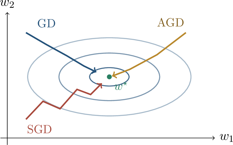
2.0.3 Nonconvexity and Overparameterization↩︎
Beyond convexity, several reassuring implications break. Global minimization is computationally hard in general; the reached solution may depend strongly on initialization, stepsize, and noise; and many different parameters may fit the training set equally well. Therefore optimization success alone does not guarantee statistical success.
The nonconvexity of neural networks has two faces. On the pessimistic side, there is no general reason that a local descent method should find a global minimum of an arbitrary nonconvex objective. On the optimistic side, overparameterization can create enough degrees of freedom that many training sets become interpolable, and gradient methods often find an interpolating solution in practice. NTK theory explains one version of this optimism: at large width, the local tangent features at initialization can already span the training labels well enough that little feature movement is needed.
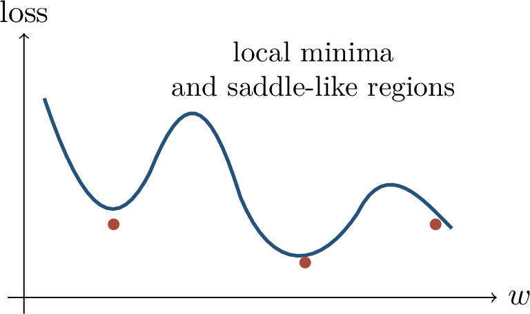
In overparameterized neural networks, \(p\gg N\) is common. The interpolation equations \[f(x_i;w)=y_i,\qquad i=1,\dots,N,\] are then underdetermined. There may be a high-dimensional set of zero-risk parameters. Optimization selects one solution from this set, and generalization depends on the implicit bias of the training path.
This observation separates two questions that are sometimes conflated. The first is whether optimization reaches small empirical risk. The second is which interpolating function it reaches. In a kernel or lazy-training regime, the answer to the second question is often a minimum-norm kernel solution. In feature-learning regimes, the answer may depend on how the internal representation changes during training.
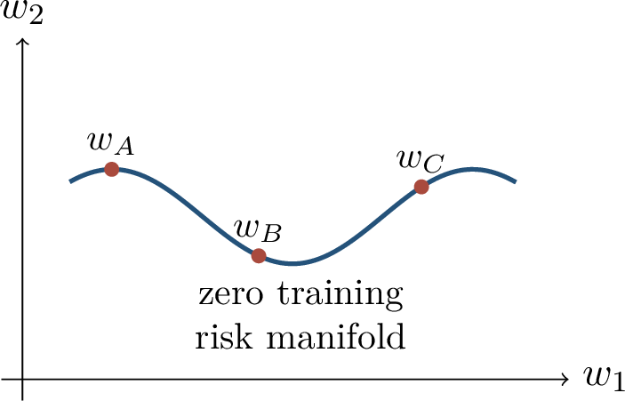
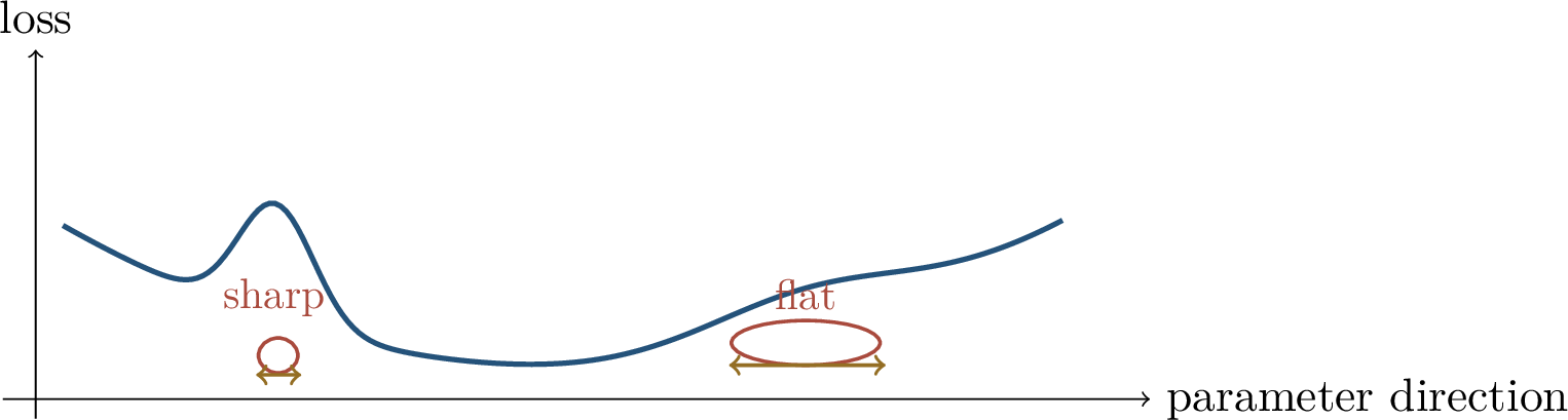
This is the setting in which one would like a theorem of the following form: for a fixed training set of size \(N\), a sufficiently wide randomly initialized network reaches zero training error if the initial tangent kernel is well conditioned and remains stable during training. The important caveats are that width bounds may be huge, kernel behavior is not full feature learning, and test error requires additional assumptions.
The phrase “well conditioned” means that the empirical tangent kernel has no nearly invisible residual direction. If \(K_0\) has a very small eigenvalue, then some linear combination of training residuals is hard to change using the initial tangent features. If \(K_0\) is uniformly positive definite and the kernel remains close to \(K_0\), then every residual direction is corrected at a controlled rate.
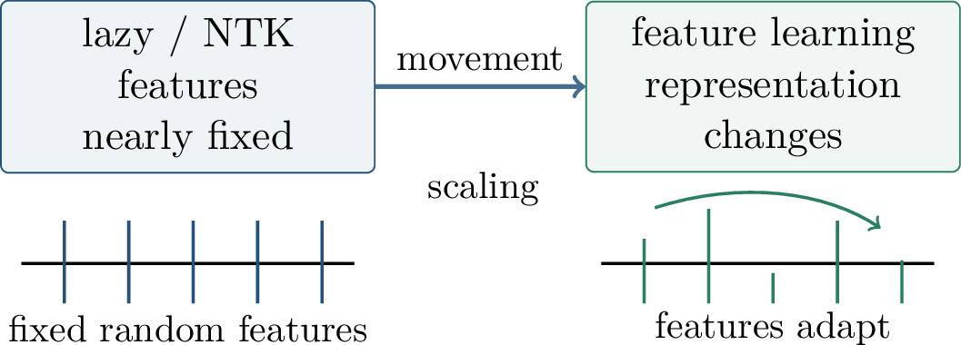
2.0.4 The Empirical Neural Tangent Kernel↩︎
Definition 0.1 (Empirical neural tangent kernel). Along a parameter trajectory \(w(t)\), define \[J_t= \begin{bmatrix} \grad_w f(x_1;w(t))^\top\\ \vdots\\ \grad_w f(x_N;w(t))^\top \end{bmatrix} \in\R^{N\times p}.\] The empirical neural tangent kernel is \[K_t=J_tJ_t^\top, \qquad K_t(i,j) = \left\langle \grad_w f(x_i;w(t)),\grad_w f(x_j;w(t)) \right\rangle.\]
The NTK measures how similarly two training examples respond to an infinitesimal parameter update. If \(K_t\) is positive definite, then every residual direction on the training set can be corrected by some parameter-space motion. This is the finite-sample object; it is a matrix, not yet a population kernel.
The definition is purely empirical. It depends on the chosen training points, the current parameter vector, and the network parameterization. The population or infinite-width NTK is obtained only after taking appropriate random-width limits. For optimization on a fixed dataset, however, the empirical matrix is the object that directly controls training-error decay.
What the NTK Matrix Measures The entry \(K_t(i,j)\) is large when examples \(x_i\) and \(x_j\) induce similar parameter gradients. A gradient step that changes the prediction on \(x_i\) will then tend to change the prediction on \(x_j\) in a related direction. The eigenvalues of the full matrix describe which collective residual directions can be removed quickly.
2.0.4.1 Scaled Gradient Flow
Let \[z(t)=\alpha f(w(t)), \qquad \mathcal{R}(z)=\frac{1}{2}\left\lVert z-y \right\rVert_2^2.\] Then \(\grad_z\mathcal{R}(z)=z-y\), and parameter-space gradient flow is \[\begin{align} \dot{w}(t) &= -\grad_w \mathcal{R}(\alpha f(w(t)))\\ &= -\alpha J_t^\top(\alpha f(w(t))-y)\\ &= -\alpha J_t^\top(z(t)-y). \end{align}\] Differentiating \(z(t)=\alpha f(w(t))\) gives the prediction-space ODE \[\begin{align} \dot{z}(t) &= \alpha J_t\dot{w}(t)\\ &= -\alpha^2J_tJ_t^\top(z(t)-y). \end{align}\] Thus the scaled empirical kernel \[\Phi(t)=\alpha^2J_tJ_t^\top\] controls risk decay: \[\dot{z}(t)=-\Phi(t)(z(t)-y).\]
This equation is the NTK analogue of the least-squares residual equation. Indeed, if \(J_t\) were replaced by a fixed matrix \(A\), then the residual \(z(t)-y\) would obey the linear ODE \(\dot{r}=-\alpha^2AA^\top r\). The only nonlinear difficulty is that \(J_t\), and therefore \(\Phi(t)\), may change as the parameters move. Lazy training is precisely the regime in which this change is small enough that the fixed-kernel intuition remains valid.
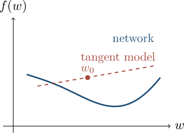
2.0.4.2 Linearization at Initialization
Near \(w_0=w(0)\), define the affine approximation \[f_0(u)=f(w_0)+J_0(u-w_0), \qquad J_0=J(w_0).\] The corresponding linearized flow freezes the Jacobian: \[\dot{u}(t) = -\alpha J_0^\top\bigl(\alpha f_0(u(t))-y\bigr).\] Let \[r_0(u)=\alpha f_0(u)-y.\] Since \(f_0\) is affine, \[r_0(u) = \alpha J_0u-\bigl(y-\alpha f(w_0)+\alpha J_0w_0\bigr).\]
The linearized model is not introduced as a new architecture to be trained in practice. It is a mathematical comparison system. If the true nonlinear trajectory remains close to the linearized trajectory, then the true network inherits the convergence behavior of the fixed-kernel model. The rest of the chapter explains what must be controlled to make this comparison rigorous.
Lemma 0.1 (Linearized NTK flow). If \(K_0=J_0J_0^\top\succ0\), then along the linearized flow, \[\require{physics} \frac{\dd}{\dd t}r_0(u(t)) = -\alpha^2K_0r_0(u(t)).\] Consequently \(r_0(u(t))\to0\) exponentially.
Proof. Differentiate \(r_0(u(t))=\alpha f_0(u(t))-y\): \[\require{physics} \frac{\dd}{\dd t}r_0(u(t)) = \alpha J_0\dot{u}(t) = -\alpha^2J_0J_0^\top r_0(u(t)).\] This is exactly the least-squares residual ODE with \(A=J_0\). ◻
The proof is short because all nonlinear terms have been removed by freezing the Jacobian. The conclusion is therefore conditional on \(K_0\succ0\). If \(K_0\) is singular, then the tangent features at initialization do not span all residual directions, and the linearized flow cannot fit arbitrary labels on the training set.
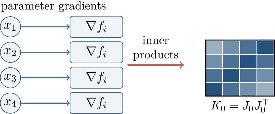
At suitable random initialization, very wide networks have two related limits: the random function \(f(\cdot;w_0)\) converges in distribution to a Gaussian process, and the empirical tangent kernel concentrates around a deterministic kernel: \[K_0(x,x')\approx K_\infty(x,x').\] In the infinite-width lazy limit, training behaves like kernel regression with this deterministic NTK.
There are two limits being compared here. The Gaussian-process limit describes the distribution of random functions at initialization. The NTK limit describes the distribution of tangent features and hence the training dynamics. Both arise from averaging many independent or weakly dependent hidden units, but they answer different questions: the first concerns the prior over functions, while the second concerns how gradient descent changes those functions.
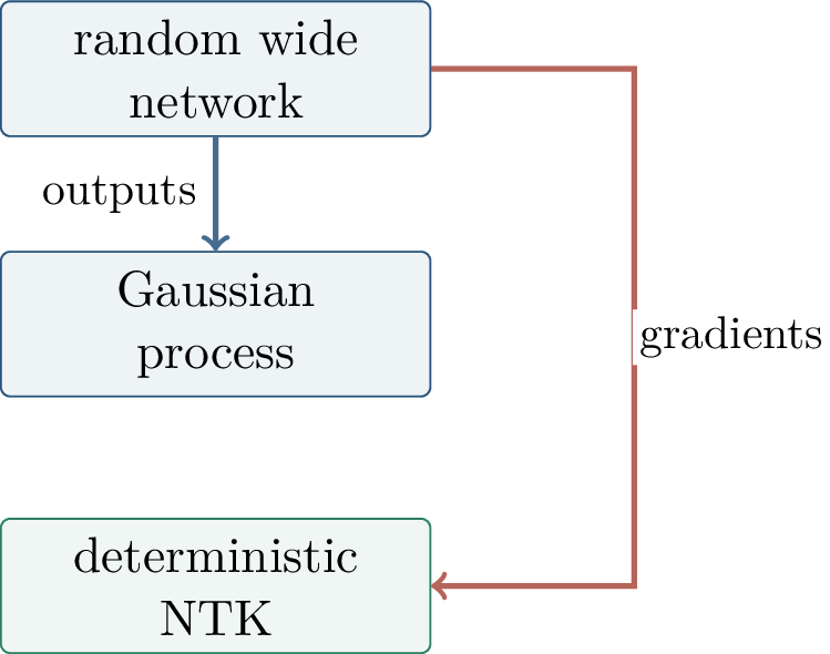
2.0.5 Convergence Mechanisms↩︎
2.0.5.1 Fixed-Kernel Decay
For the linearized flow, the kernel \(K_0\) is constant: \[\dot{r}(t)=-\alpha^2K_0r(t), \qquad r(t)=e^{-\alpha^2K_0t}r(0).\]
The spectral picture is completely explicit. Each eigenvector of \(K_0\) defines a residual mode. Large eigenvalues correspond to modes that are quickly removed by gradient flow; small eigenvalues correspond to slow modes. The minimum eigenvalue is therefore a worst-case training-speed parameter. This is why finite-sample NTK analyses typically assume, or prove with high probability, that \(\lambda_{\min}(K_0)\) is bounded below.
Theorem 0.1 (Linearized convergence). If \(\lambda_{\min}(K_0)\ge\sigma_{\min}>0\), then \[\left\lVert r(t) \right\rVert \le \left\lVert r(0) \right\rVert e^{-\alpha^2\sigma_{\min}t},\] and \[\mathcal{R}(t) \le \mathcal{R}(0)\exp(-2\alpha^2\sigma_{\min}t).\]
Proof. Diagonalize \(K_0=Q\Lambda Q^\top\). In the eigenbasis, every residual component satisfies \[\require{physics} \frac{\dd}{\dd t}\widetilde{r}_i(t) = -\alpha^2\lambda_i\widetilde{r}_i(t), \qquad \widetilde{r}_i(t)=e^{-\alpha^2\lambda_i t}\widetilde{r}_i(0).\] Since every \(\lambda_i\ge\sigma_{\min}\), the displayed norm and risk bounds follow. ◻
2.0.5.2 Moving Kernels
For the true nonlinear network, \[\dot{z}(t)=-\Phi(t)(z(t)-y), \qquad \Phi(t)=\alpha^2J_tJ_t^\top.\] The only difference from the linearized residual ODE is that \(\Phi(t)\) now changes with time. If it remains uniformly positive definite, the same exponential decay argument still works.
This statement is stronger than it first appears. The kernel does not have to be exactly fixed. It may move, and the features may drift, as long as the matrix never loses its positive-definite lower bound. Thus the proof of optimization reduces to a stability problem: show that the trajectory remains inside a region where the empirical NTK is still well conditioned.
Lemma 0.2 (Risk decay with a moving kernel). Suppose \[\Phi(t)\succeq \lambda I\] for all \(t\in[0,\tau]\). Then \[\mathcal{R}(z(t)) \le \mathcal{R}(z(0))e^{-2\lambda t}, \qquad 0\le t\le\tau.\]
Proof. Since \(\mathcal{R}(z)=\frac{1}{2}\left\lVert z-y \right\rVert^2\), \[\require{physics} \begin{align} \frac{\dd}{\dd t}\mathcal{R}(z(t)) &= \left\langle \dot{z}(t),z(t)-y \right\rangle\\ &= -\left\langle \Phi(t)(z(t)-y),z(t)-y \right\rangle\\ &\le -\lambda\left\lVert z(t)-y \right\rVert^2 =-2\lambda\mathcal{R}(z(t)). \end{align}\] Gronwall’s inequality gives the stated bound. The reference notes emphasize this step because it converts a matrix lower bound on \(\Phi(t)\) into a risk bound. ◻
The reference notes also phrase the preceding step using a simple comparison principle: if a scalar quantity \(u\) obeys \(\dot{u}(t)\le \beta(t)u(t)\), then \[\require{physics} u(t)\le u(0)\exp\!\left(\int_0^t \beta(s)\,\dd s\right).\] For \(\beta(t)=-2\lambda\), this is precisely the exponential risk decay above.
The comparison principle is one of the main conveniences of gradient flow. Rather than solving the nonlinear ODE for \(z(t)\), it is enough to upper bound the derivative of the scalar risk. This converts a matrix-valued stability condition into a one-dimensional differential inequality.
2.0.5.3 Bounding Parameter Motion
Risk decay is only half of the lazy-training argument. We also need to show that the parameters do not move far; otherwise the Jacobian might change substantially and the kernel lower bound might fail.
The logic is circular unless handled carefully. To prove risk decay, we want the kernel to remain positive definite. To prove the kernel remains positive definite, we want the parameters to remain close to initialization. To prove small parameter movement, we use risk decay. Lazy-training proofs close this loop by a bootstrap: assume stability on a maximal time interval, derive a movement bound that improves the stability assumption, and conclude that the interval extends through the whole training trajectory.
Let \[g(v)=\alpha f(v), \qquad S(t)=\alpha J_t, \qquad \Phi(t)=S(t)S(t)^\top.\] Consider the flow \[\dot{v}(t)=-S(t)^\top(g(v(t))-y).\]
Lemma 0.3 (Trajectory length bound). Assume that on \([0,\tau]\), \[\lambda I\preceq \Phi(t)\preceq \lambda_{\max}I.\] Then \[\left\lVert v(t)-v(0) \right\rVert \le \frac{\sqrt{\lambda_{\max}}}{\lambda} \left\lVert g(v(0))-y \right\rVert = \frac{\sqrt{2\lambda_{\max}\mathcal{R}(g(v(0)))}}{\lambda} \qquad (0\le t\le\tau).\]
Proof. Integrating the speed gives \[\require{physics} \begin{align} \left\lVert v(t)-v(0) \right\rVert &\le \int_0^t\left\lVert \dot{v}(s) \right\rVert\,\dd s\\ &= \int_0^t\left\lVert S(s)^\top(g(v(s))-y) \right\rVert\,\dd s\\ &\le \sqrt{\lambda_{\max}} \int_0^t\left\lVert g(v(s))-y \right\rVert\,\dd s . \end{align}\] The lower bound \(\Phi(s)\succeq\lambda I\) implies \[\left\lVert g(v(s))-y \right\rVert \le \left\lVert g(v(0))-y \right\rVert e^{-\lambda s}\] by the moving-kernel risk estimate. Therefore \[\require{physics} \left\lVert v(t)-v(0) \right\rVert \le \sqrt{\lambda_{\max}}\left\lVert g(v(0))-y \right\rVert \int_0^t e^{-\lambda s}\,\dd s \le \frac{\sqrt{\lambda_{\max}}}{\lambda} \left\lVert g(v(0))-y \right\rVert.\] ◻
Combining the two estimates gives the form emphasized in the chapter. Suppose that on a time interval \[\alpha^2\sigma_{\min}I \preceq \Phi(t) \preceq \alpha^2\sigma_{\max}I.\] Then \[\mathcal{R}(\alpha f(w(t))) \le \mathcal{R}(\alpha f(w(0)))e^{-2\alpha^2\sigma_{\min}t},\] and \[\left\lVert w(t)-w(0) \right\rVert \le \frac{\sqrt{2\sigma_{\max}\mathcal{R}(\alpha f(w(0)))}}{\alpha\sigma_{\min}}.\] Large \(\alpha\) makes prediction-space training fast while making parameter-space movement small. This is the basic lazy-training tradeoff.
This formula also explains why width behaves like a stabilizing scale in many NTK proofs. Under standard normalizations, increasing width averages many tangent features and concentrates the initial kernel; after rescaling, the same prediction change can be achieved with smaller motion of each parameter. The network learns in prediction space while remaining near its initial features in parameter space.
Bootstrap Template Prove three facts: \(K_0\) is well conditioned at initialization; if the parameters stay near \(w_0\), then \(K_t\) remains close to \(K_0\); if \(K_t\) remains well conditioned, then risk decays and the parameters stay near \(w_0\). These implications close the lazy-training argument.
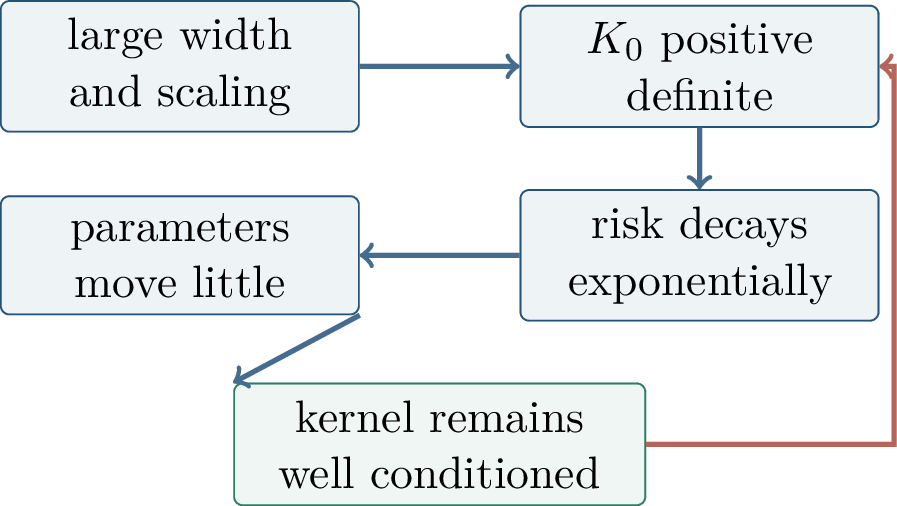
2.0.6 Random Features, Adaptive Features, and Width↩︎
The simplest model behind the NTK proof is a random-features model: \[f(x;a)=\frac{1}{\sqrt m}\sum_{r=1}^m a_r\sigma(b_r^\top x),\] where only the output weights \(a_r\) are trained and the random hidden weights \(b_r\) are fixed. The model is linear in \(a\), with feature matrix \[\Psi_{ir}=\frac{1}{\sqrt m}\sigma(b_r^\top x_i).\] Training this model is exactly least squares in the feature matrix \(\Psi\).
Random features are the cleanest bridge between neural networks and kernel methods. The hidden layer produces a random finite-dimensional feature map, and training only the last layer chooses a linear combination of these features. As \(m\) grows, the empirical feature kernel \(\Psi\Psi^\top\) concentrates around the kernel obtained by averaging over the random hidden weights. No feature learning occurs in this model; all learning is in the output coefficients.
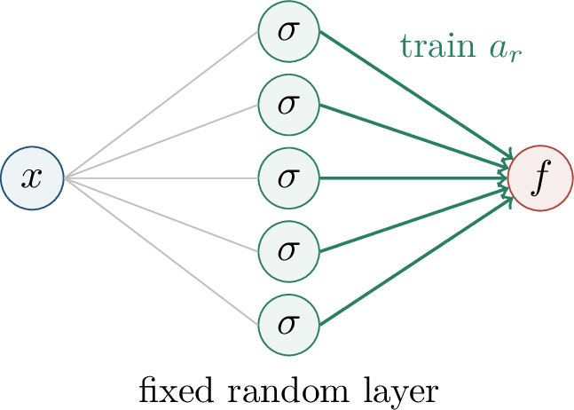
For a two-layer neural network with trainable hidden features, \[f(x;w)=\frac{1}{\sqrt m}\sum_{r=1}^m a_r\sigma(b_r^\top x),\] the tangent kernel has two types of contributions: \[K_0(x,x')=K_a(x,x')+K_b(x,x').\] The \(K_a\) part comes from changing output weights, while \(K_b\) comes from moving hidden features. In the NTK regime, the network is wide enough that these tangent features remain nearly fixed during training. Beyond NTK, hidden features move substantially, and the analysis must track representation learning rather than only kernel regression.
This decomposition clarifies what the tangent kernel contains. Even when all parameters are trainable, the NTK describes the infinitesimal effect of moving them at initialization. It includes tangent directions associated with hidden weights, but in the lazy regime those tangent directions themselves do not change much. Thus NTK training can use a richer kernel than a pure random-features model while still remaining a fixed-feature theory.
2.0.6.1 Why Width Behaves Like a Scale
The chapter uses the heuristic \[\text{large width} \approx \text{large }\alpha \Longrightarrow \text{small movement} \Longrightarrow \text{stable NTK}.\] One thought experiment is to duplicate features. Duplicating a network creates a wider model with the same tangent directions but more averaged random features. As width grows, fluctuations in the empirical kernel shrink, and the tangent matrix concentrates around a deterministic limit.
The \(1/\sqrt m\) normalization is essential in this discussion. It keeps the output variance of the random network of constant order as \(m\) changes. At the same time, individual units contribute only a small amount, so moving any single unit has a small effect on the function. Width therefore produces both concentration of the initial kernel and stability of the tangent features under gradient flow.
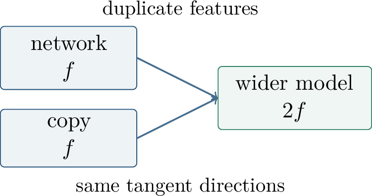
For fully connected layers of widths \(n_i\), the NTK regime uses variance-preserving initialization \[x\mapsto A_ix+b_i, \qquad A_i=\frac{1}{\sqrt{n_i}}W_i,\] where the entries of \(W_i\) are independent standard Gaussian variables at initialization. Under such scaling, as hidden widths go to infinity, both outputs and tangent kernels concentrate. The reference notes also point toward the mean-field view, where a different scaling describes feature dynamics through a limiting PDE; that topic belongs to later chapters.
2.0.6.2 Kernel Regression View
If the NTK is fixed at \(K_0\), then the learned prediction satisfies \[z(t)-y=e^{-\alpha^2K_0t}(z(0)-y).\] As \(t\to\infty\), the training predictions interpolate the labels. Among interpolating predictors, the corresponding function-space solution is the minimum-norm solution in the reproducing kernel Hilbert space associated with the fixed kernel. Thus overparameterized neural-network optimization becomes, in this regime, a problem in kernel methods.
This viewpoint is useful but also limiting. Kernel regression can explain fast training and a particular implicit bias, but it does not describe the formation of new internal representations. If a practical network improves because hidden features rotate, specialize, or become invariant to nuisance directions, then a fixed NTK is not the right complete model. The value of NTK theory is that it gives a rigorous reference regime against which feature learning theories can be compared.
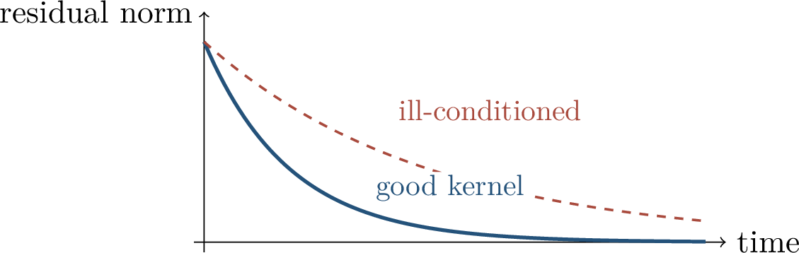
2.0.7 What NTK Theory Explains↩︎
NTK theory explains why sufficiently wide random networks can fit finite training sets, why least-squares residual dynamics reappear inside neural network training, and why the smallest empirical NTK eigenvalue controls the training speed. The proof strategy is clear: show that the initial tangent kernel is positive definite; prove that risk decays if the kernel remains positive definite; use the trajectory-length bound to show that, with enough width and scaling, the parameters move so little that the kernel remains close to its initial value.
The theory does not fully explain representation learning in practical finite-width networks, transfer across tasks, robustness, invariance, or data-dependent feature formation. The reference notes make this point in a practical way: infinite-width kernel methods can be useful and analytically computable, but choosing every architecture to be literally infinitely wide is not the goal. The NTK regime gives a rigorous kernel-based algorithmic lens, not the final theory of deep learning.
Chapter Synthesis The NTK turns finite-sample training into prediction-space dynamics. In the linearized regime, residuals decay according to a fixed Gram matrix \(K_0=J_0J_0^\top\). For the nonlinear network, convergence follows if the moving kernel remains uniformly positive definite. Wide-network lazy-training proofs close this argument by showing that parameter movement is small enough to keep the kernel stable.
Primary references for this chapter include the neural tangent kernel paper of Jacot, Gabriel, and Hongler [8]; convergence analyses for overparameterized neural networks such as [9], [10]; the lazy-training perspective of Chizat, Oyallon, and Bach [27]; and the result of Lee et al. that wide networks evolve as linear models under gradient descent [26]. These references support the fixed-kernel and lazy-training viewpoint developed in this chapter.
2.0.8 Why Optimizer Design Is Part of the Theory↩︎
The previous chapter studied gradient flow, neural tangent kernels, and the conditions under which wide neural networks can be optimized. The next chapter studies implicit regularization: when many parameter vectors fit the training set, which one does the algorithm find? This chapter sits exactly between those two questions. Adaptive optimizers change the metric in which descent is performed, the statistics by which noisy gradients are averaged, and the systems cost of training a large model.
Modern deep learning practice does not treat the optimizer as a neutral implementation detail. The optimizer is part of the model-training system. It affects the path through parameter space, the scale of each parameter group, the amount of memory needed per parameter, and the tuning burden for large-scale runs.
This is a conceptual shift from the clean gradient-flow picture of the previous chapter. In Euclidean gradient descent, the negative gradient is the steepest descent direction measured in the ordinary Euclidean norm. Adaptive methods change that norm, often coordinate by coordinate and time step by time step. As a result, two optimizers can see the same stochastic gradients and yet follow different paths, reach different interpolating solutions, and use different amounts of memory. Optimizer design is therefore not only an engineering choice; it is a choice of geometry, noise filtering, and implicit bias.
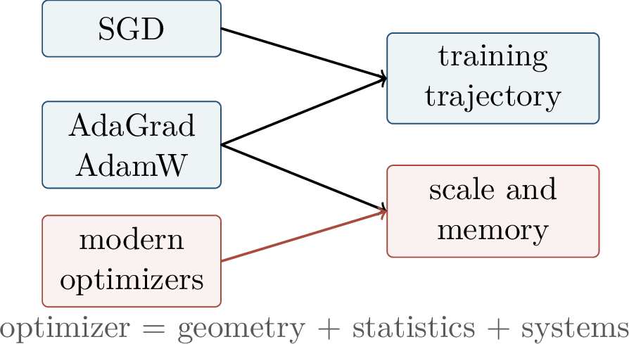
The guiding question is:
How do adaptive optimizers change geometry, implicit bias, and the cost of training foundation models?
The answer is not a single theorem. Rather, the chapter develops a sequence of models. AdaGrad gives a clean convex and online-learning picture of coordinate adaptivity. Adam replaces infinite memory by exponential moving averages and becomes the practical default. AMSGrad explains a convergence repair. AdamW separates optimization from weight decay. Finally, modern large-model optimizers revisit the same themes under severe memory and communication constraints.
The historical arc is also instructive. AdaGrad was introduced as an adaptive subgradient method with regret guarantees in online convex optimization [30]. Adam combined momentum and adaptive second moments into a practical stochastic optimizer [31]. AMSGrad was proposed after examples showed that Adam’s moving denominator can break convergence in simple convex settings [32]. AdamW then separated weight decay from the adaptive update, restoring the meaning of multiplicative shrinkage for adaptive methods [33].
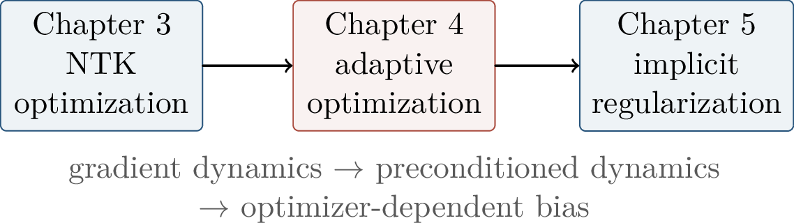
Definition 0.2 (Preconditioned stochastic descent). Let \[f(\theta)=\E_{\xi\sim\mathcal{D}}\ell(\theta;\xi), \qquad g_t\approx \nabla f(\theta_t)\] be a stochastic gradient. A preconditioned stochastic descent method has the form \[\theta_{t+1}=\theta_t-\eta_t P_t g_t, \qquad P_t\succeq 0.\] Here \(P_t\) may be fixed, data-dependent, diagonal, low-rank, or a richer matrix preconditioner.
This template lets us compare optimizers in a common language. SGD corresponds to \(P_t=I\). AdaGrad and Adam use diagonal, history-dependent preconditioners. Matrix methods such as Shampoo-like optimizers use richer layer structure. Memory-efficient methods approximate the same idea while reducing optimizer state.
When \(P_t\) is positive definite, the update is the steepest descent direction for a local quadratic geometry. More precisely, the vector \(-P_tg_t\) is the solution of \[\min_{\Delta} \left\{ \left\langle g_t,\Delta \right\rangle +\frac{1}{2\eta_t}\left\lVert \Delta \right\rVert_{P_t^{-1}}^2 \right\}.\] Thus the preconditioner changes the cost of moving in different directions. Diagonal adaptive methods are inexpensive because they rescale coordinates independently; the price is that they cannot represent correlations between parameters.
Optimizer as Geometry An optimizer is not only a rule for choosing a stepsize. It specifies a time-dependent geometry in parameter space, a statistical estimator of useful gradient information, and a memory budget for storing that information.
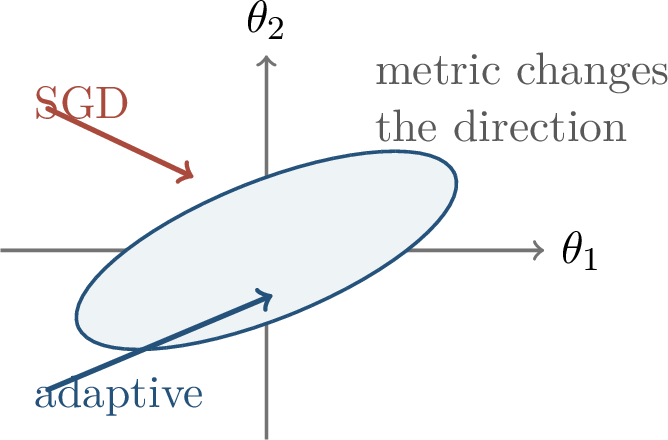
The chapter is organized around three axes.
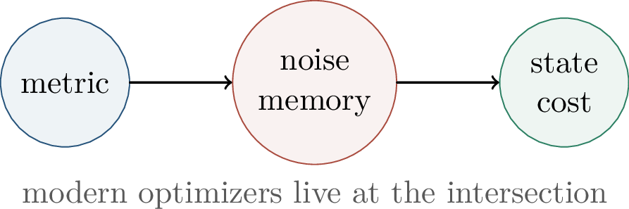
2.0.9 AdaGrad and Data-Dependent Geometry↩︎
AdaGrad is the cleanest starting point because it has a simple online-learning interpretation. At round \(t\), an algorithm chooses \(\theta_t\), observes a loss \(\ell_t\), and receives a gradient \(g_t=\nabla \ell_t(\theta_t)\). The algorithm is compared with a fixed decision \(u\) using regret \[R_T(u)=\sum_{t=1}^T \ell_t(\theta_t)-\ell_t(u).\] Small regret means that the sequence of decisions performs nearly as well as the best fixed comparator chosen in hindsight.
The online formulation is useful even when our eventual goal is stochastic neural-network training. It forces us to ask what information the algorithm has when it chooses a step. AdaGrad uses only past gradients, and it converts their coordinate-wise magnitudes into a changing metric. If a coordinate has already received many large gradients, the algorithm treats future motion in that coordinate as expensive. If a coordinate has been quiet, the algorithm keeps a larger effective step available.
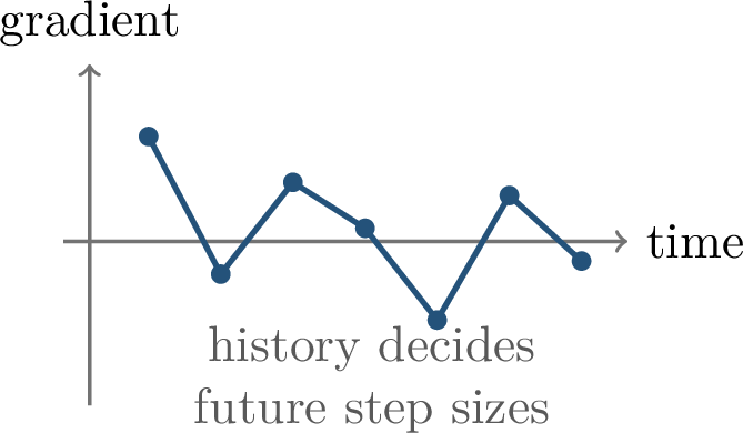
Definition 0.3 (Diagonal AdaGrad). Initialize \(s_0=0\). Given a gradient \(g_t\in\R^d\), AdaGrad updates \[s_t=s_{t-1}+g_t\odot g_t, \qquad \theta_{t+1} = \theta_t-\eta\, \frac{g_t}{\sqrt{s_t}+\varepsilon},\] where the square root and division are coordinate-wise.
Coordinate \(j\) has effective learning rate \[\eta_{t,j}^{\mathrm{eff}} = \frac{\eta}{\sqrt{s_{t,j}}+\varepsilon}.\] Thus frequent or high-magnitude gradients reduce future steps in the same coordinate, while rare coordinates keep larger steps.
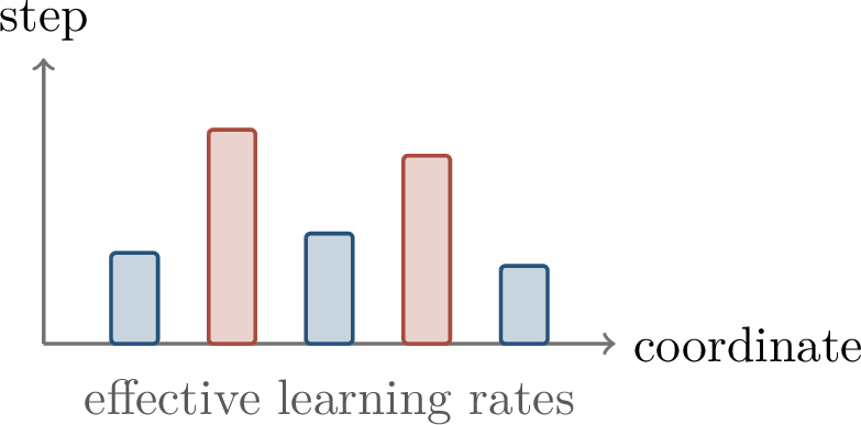
Theorem 0.2 (AdaGrad coordinate-form regret bound). For convex \(G_\infty\)-Lipschitz losses on a bounded domain of diameter \(D\), diagonal AdaGrad satisfies a regret bound of the form \[R_T(u) \;\lesssim\; \left(\frac{D^2}{\eta}+\eta\right) \sum_{j=1}^d \sqrt{\sum_{t=1}^T g_{t,j}^2}.\] The important point is that the bound depends on the observed coordinate-wise gradient history, not only on \(d\) and \(T\).
The theorem is often more illuminating than its constants. If only a few coordinates accumulate significant gradients, the sum \(\sum_j\sqrt{\sum_t g_{t,j}^2}\) can be much smaller than a dimension-blind worst-case bound. AdaGrad is therefore a method for matching the update geometry to the data seen so far.
To see the comparison with a dimension-blind bound, suppose \(\left\lVert g_t \right\rVert_2\le G\). Cauchy’s inequality gives \[\sum_{j=1}^d \sqrt{\sum_{t=1}^T g_{t,j}^2} \le \sqrt{d\sum_{j=1}^d\sum_{t=1}^T g_{t,j}^2} \le G\sqrt{dT}.\] This recovers the familiar \(\sqrt{dT}\)-type dependence. The value of AdaGrad is that the actual bound can be much smaller when the observed gradient sequence is sparse or anisotropic. The algorithm therefore adapts to the geometry of the realized data, not only to a worst-case dimension.
Definition 0.4 (AdaGrad metric). Let \[G_t=\diag(\sqrt{s_t}+\varepsilon).\] The norm \(\left\lVert x \right\rVert_{G_t}^2=x^\top G_t x\) makes directions with large historical gradients expensive. AdaGrad can be interpreted as a mirror descent or steepest descent method in this changing data-dependent norm.
This metric interpretation is often the most transferable lesson from AdaGrad. The algorithm is not merely reducing learning rates over time. It is changing the coordinate system in which a unit step is measured. A coordinate with accumulated squared gradient \(s_{t,j}\) has metric weight \(\sqrt{s_{t,j}}+\varepsilon\), so a displacement in that coordinate costs more in the local norm. This is why AdaGrad can be viewed as a diagonal approximation to second-order geometry, although its statistic is based on gradient history rather than on the Hessian.
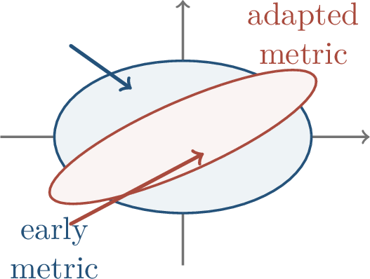
Example 0.1 (Rare but predictive features). Suppose \(x_1\) is a frequent noisy feature and \(x_2\) is a rare but predictive feature. A global learning rate treats their coordinates symmetrically. AdaGrad can reduce steps along the frequently excited noisy coordinate while preserving larger steps for the rare coordinate.
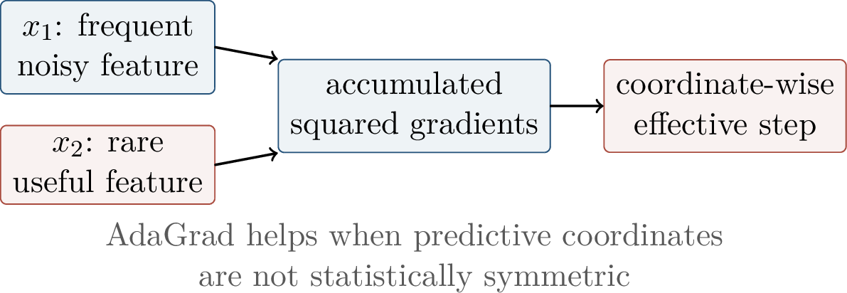
AdaGrad also has limitations. Its classical regret theory is convex or online; deep networks are nonconvex. Diagonal scaling ignores correlations between parameters. The accumulated sum \(s_t=\sum_{\tau\le t}g_\tau^2\) never forgets, so late training can become too conservative. Adam replaces this infinite memory by exponential memory.
What AdaGrad Teaches AdaGrad shows that adaptivity can be theoretically meaningful when the gradient sequence is anisotropic. Its regret bound rewards sparse or uneven coordinate activity. Its weakness is equally clear: a denominator that only increases may become too conservative in long nonconvex training runs.
2.0.10 Adam, AMSGrad, and AdamW↩︎
Adam combines two ideas: momentum for the first moment and RMS normalization for the second moment. It is best viewed as a diagonal preconditioner whose statistics are computed from a finite effective memory window.
The first moment \(m_t\) smooths the stochastic gradient direction. The second moment \(v_t\) estimates coordinate-wise gradient scale and turns that scale into an adaptive denominator. The parameters \(\beta_1\) and \(\beta_2\) determine effective memory lengths: roughly speaking, \((1-\beta_1)^{-1}\) and \((1-\beta_2)^{-1}\) steps. In common settings \(\beta_2\) is much closer to one than \(\beta_1\), so the denominator changes more slowly than the momentum direction.
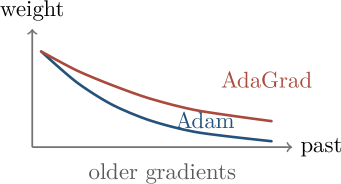
Definition 0.5 (Adam). Given parameters \(\beta_1,\beta_2\in[0,1)\), initialize \(m_0=v_0=0\). Adam computes \[\begin{align} m_t &= \beta_1 m_{t-1}+(1-\beta_1)g_t,\\ v_t &= \beta_2 v_{t-1}+(1-\beta_2)(g_t\odot g_t),\\ \widehat m_t &= \frac{m_t}{1-\beta_1^t}, \qquad \widehat v_t = \frac{v_t}{1-\beta_2^t},\\ \theta_{t+1} &= \theta_t-\eta \frac{\widehat m_t}{\sqrt{\widehat v_t}+\varepsilon}. \end{align}\] The vector \(m_t\) estimates the first moment, and \(v_t\) estimates the coordinate-wise second moment.
The bias corrections compensate for the fact that the moving averages start at zero. The informal slogan is: momentum chooses a direction, while RMS normalization chooses units.
For example, if the stochastic gradients have constant mean \(g\), then \[\E[m_t]=(1-\beta_1^t)g.\] Dividing by \(1-\beta_1^t\) removes the initialization bias. The same calculation applies coordinate-wise to \(v_t\) when the second moment is stationary. This correction is most important in the first few iterations, exactly when the moving averages are still close to their zero initialization.
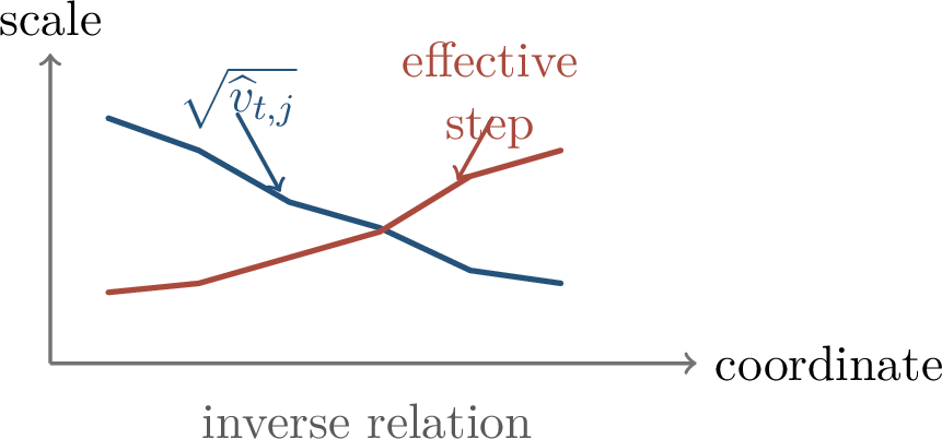
For coordinate \(j\), \[\eta_{t,j}^{\mathrm{eff}} = \frac{\eta}{\sqrt{\widehat v_{t,j}}+\varepsilon}.\] Flat or low-gradient coordinates can receive larger steps; high-variance coordinates receive smaller steps.
This normalization is the source of both Adam’s robustness and its subtlety. It makes the update relatively insensitive to the scale of a coordinate’s gradient, which helps tuning across heterogeneous parameter groups. But it also means that a coordinate with tiny recent variance can suddenly receive a large effective step. Theoretical convergence therefore depends on how the denominator evolves over time, not just on whether the instantaneous gradient points in a good direction.
Theorem 0.3 (Adam can fail to converge, informal). There are simple convex online optimization instances where Adam’s moving second moment makes effective steps non-monotone, and the iterates do not converge to the optimum.
The issue is not merely stochasticity. A coordinate may receive a large step after its estimated variance drops, even if earlier gradients suggested that the coordinate should remain conservative. Reddi, Kale, and Kumar showed that enforcing a nondecreasing denominator gives a clean repair.
The counterexamples behind this theorem are deliberately simple: they show that even in convex online problems, Adam’s exponentially weighted second moment can forget a large past gradient quickly enough to make later updates too aggressive. Thus the problem is structural rather than an artifact of deep-network nonconvexity. AMSGrad fixes the structure by replacing the raw second-moment estimate with a coordinate-wise running maximum.
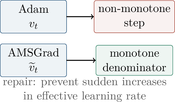
Definition 0.6 (AMSGrad). AMSGrad modifies Adam by setting \[\widetilde{v}_t=\max(\widetilde{v}_{t-1},\widehat v_t), \qquad \theta_{t+1} = \theta_t-\eta \frac{\widehat m_t}{\sqrt{\widetilde{v}_t}+\varepsilon},\] where the maximum is coordinate-wise.
AMSGrad is important theoretically, but AdamW is more common in large-scale language-model practice. The central difference is the treatment of weight decay.
AMSGrad is conservative: once a coordinate’s denominator has become large, it cannot decrease. This monotonicity helps the regret analysis, but it also removes some of the adaptivity that made Adam attractive in long training runs. In practice, the AdamW modification addresses a different issue that appears whenever adaptive normalization and regularization are mixed.
Definition 0.7 (AdamW). AdamW decouples weight decay from the adaptive gradient update: \[\theta_{t+1} = (1-\eta\lambda)\theta_t - \eta \frac{\widehat m_t}{\sqrt{\widehat v_t}+\varepsilon}.\] The shrinkage term bypasses the adaptive denominator.
For SGD with a fixed learning rate, adding \(\lambda\theta_t\) to the gradient can look like weight decay. For adaptive methods this equivalence breaks: the term \(\lambda\theta_t\) would be divided by \(\sqrt{\widehat v_t}+\varepsilon\), so different coordinates would receive different regularization strengths. AdamW restores the idea of multiplicative decay by separating the channels.
This distinction is easiest to see in one coordinate. Coupled \(L_2\) regularization inside Adam would update \[\theta_{t+1,j} = \theta_{t,j} - \eta \frac{\widehat m_{t,j}+\lambda\theta_{t,j}}{\sqrt{\widehat v_{t,j}}+\varepsilon},\] so the shrinkage depends on the stochastic gradient scale of that coordinate. AdamW instead applies the multiplicative factor \(1-\eta\lambda\) outside the adaptive denominator. The regularization strength is therefore controlled by \(\lambda\) and the learning rate, rather than by the recent gradient history.
Adam, AMSGrad, AdamW Adam is a practical exponentially weighted adaptive method. AMSGrad is a theoretical repair that prevents the denominator from decreasing. AdamW is a regularization repair: it decouples weight decay from the adaptive gradient preconditioner.
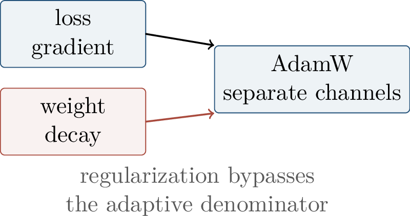
2.0.11 Implicit Bias and Generalization↩︎
In overparameterized learning, many parameter vectors can interpolate the training data. The optimizer selects a path to one of them. Adaptive methods can therefore change not only the training speed but also the solution reached at zero training error.
This point connects directly to implicit regularization. Explicit regularization is written in the objective, such as a norm penalty. Implicit regularization is induced by the algorithm: initialization, stepsize, noise, preconditioning, momentum, and stopping time can all affect which solution is selected from a large interpolating set. Adaptive methods introduce a particularly visible source of implicit bias because they rescale coordinates based on the gradient history.

There are learning problems where adaptive gradient methods reach zero training error but converge to a classifier with worse test error than the one found by SGD.
The proposition, inspired by Wilson et al., is a warning rather than a universal indictment of adaptive methods. Adaptivity can emphasize rare or high-gradient coordinates. This helps when such coordinates are informative, but it can hurt when they are spurious.
Wilson et al. [34] used such examples to argue that the marginal value of adaptive methods is not captured by training error alone. The same mechanism can be beneficial or harmful depending on the data distribution. If rare coordinates are stable signal, adaptivity can find them quickly. If rare coordinates are shortcuts that disappear at test time, adaptivity can overemphasize them and generalize worse than a less adaptive method.
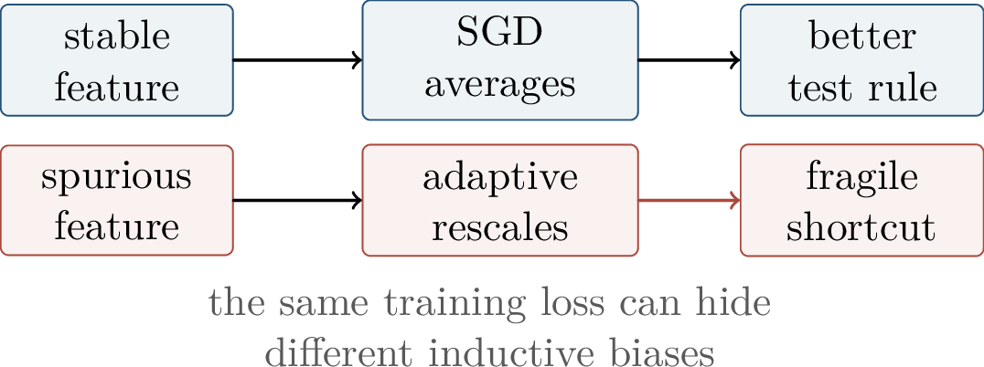
Scale invariance adds another complication. For a ReLU unit, \[a\,\sigma(w^\top x) = (ca)\,\sigma((w/c)^\top x), \qquad c>0.\] Many parameterizations represent the same function. An optimizer that is not invariant to this rescaling can prefer one representation over another even when the represented function is unchanged.
This matters because adaptive optimizers are parameterization-dependent. Changing the scale of one layer and compensating in the next layer can leave the network function unchanged, but the coordinate-wise gradient magnitudes and moment estimates may change. Thus a statement about “the optimizer’s implicit bias” is incomplete unless the parameterization and normalization conventions are specified.
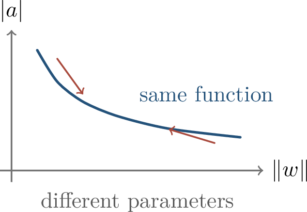
Definition 0.8 (Gradient flow with a metric). For a time-dependent positive semidefinite matrix \(P(t)\), the continuous time analogue of preconditioned descent is \[\dot{\theta}(t)=-P(t)\nabla f(\theta(t)).\] The choice of \(P(t)\) changes the trajectory even when the objective is the same.
In continuous time, the metric view makes optimizer dependence explicit. If \(P(t)=I\), the trajectory follows Euclidean gradient flow. If \(P(t)\) is a diagonal matrix built from gradient history, coordinates are stretched or compressed before the step is taken. If \(P(t)\) is a matrix preconditioner, the flow can rotate directions as well as rescale them. All three flows can decrease the same objective while selecting different interpolating points.
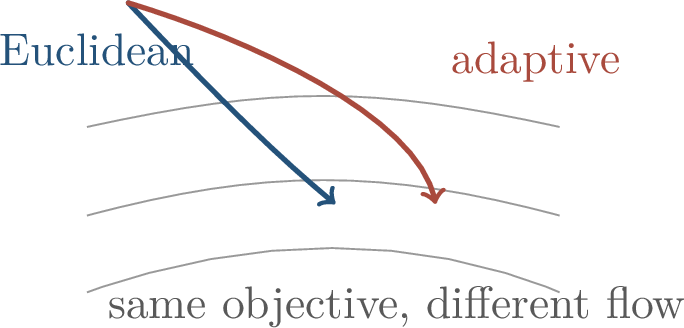
Once the training loss is nearly zero, the optimizer still matters because it determines the route to interpolation. SGD has noise-induced and geometry-induced biases; AdaGrad and Adam introduce coordinate-wise rescaling; AdamW separates shrinkage from the adaptive gradient path. These ideas feed directly into the next chapter on implicit regularization.
Generalization Warning Adaptive optimization is not automatically better or worse for test error. It changes the path and the selected solution. Whether that change is helpful depends on the alignment between adaptive coordinates and stable predictive structure in the data.
2.0.12 Transformers and Optimizer State at Scale↩︎
Transformer training made AdamW the default optimizer in much of modern deep learning. A transformer contains embeddings, attention matrices, MLP blocks, and normalization parameters whose gradient scales can differ sharply. A single global SGD learning rate is difficult to tune across all these groups. AdamW supplies many effective learning rates while maintaining a stable decay rule.
The difficulty is not only that transformers are large. Their parameters play different functional roles. Embedding tables, attention projections, MLP weights, normalization parameters, and output heads can have different gradient distributions and different sensitivity to decay. Adaptive optimizers offer a pragmatic compromise: they keep one global algorithmic framework while allowing local effective learning rates to vary across coordinates and blocks.
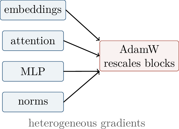
The same adaptivity that helps tuning also increases memory. For \(N\) parameters, Adam-style training stores the parameters, gradients, first moments, and second moments, plus mixed-precision copies and distributed communication buffers.
This memory cost is often the real bottleneck. If each parameter has a first moment and a second moment, the optimizer state alone is already on the order of twice the parameter count. Mixed-precision training may keep master weights in higher precision, and distributed training may add communication or partitioning metadata. At foundation-model scale, saving a constant factor in optimizer state can decide whether a training run fits on available hardware.
| Method | Extra state | Main idea |
|---|---|---|
| SGD + momentum | \(1\times\) | store a first moment |
| AdamW | \(2\times\) | store first and second moments |
| Adafactor | sublinear blocks | factor second-moment statistics |
| GaLore / LoRA-Pre | low-rank state | project optimizer memory |
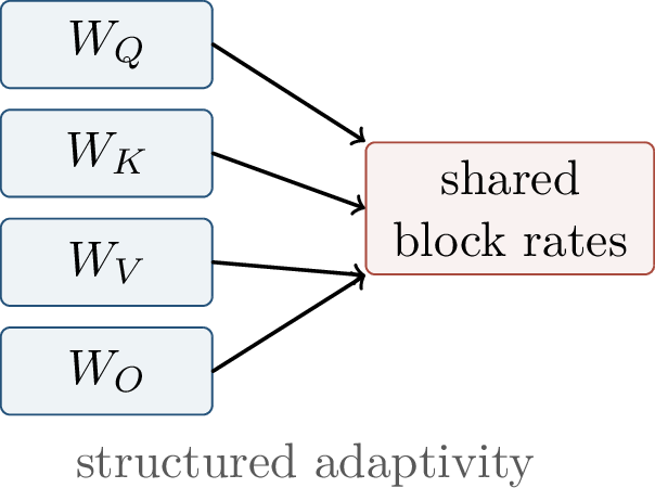
Adam-mini is motivated by the observation that many coordinates in a large language model may not need separate second-moment learning-rate resources. Structured parameter blocks can share some effective rates, reducing memory while preserving Adam-like behavior where it matters most.
The tradeoff is between statistical resolution and memory. A fully diagonal Adam-style denominator assigns one statistic to every coordinate. A block-shared method assumes that some coordinates have sufficiently similar scale behavior that they can share a statistic. This is a modeling assumption about optimizer geometry, just as convolution or attention is a modeling assumption about functions.
Definition 0.9 (Adafactor moment factorization). For a matrix-shaped parameter \(W\in\R^{r\times c}\), Adafactor approximates a dense second-moment matrix \(V\) using row and column statistics: \[V \approx \frac{RC^\top}{\operatorname{mean}(R)}.\] The memory cost becomes \(O(r+c)\) rather than \(O(rc)\).
The approximation is meaningful when the second-moment structure has strong row and column components. It is not a free replacement for a full diagonal statistic: correlations and irregular coordinate effects may be lost. The reason Adafactor-style ideas are attractive is that the memory reduction is asymptotically large for matrix parameters, while the retained row and column statistics often capture useful scale information.
Another route is to reduce the optimizer state by projecting gradients onto low-dimensional subspaces.
Low-rank optimizer-state methods make a different assumption. Instead of sharing statistics by rows and columns, they assume that the most important gradient variation lives in a low-dimensional subspace. The optimizer stores state after projection, updates in that subspace, and periodically refreshes or adapts the projection. The mathematical question is how much training signal is lost by the projection and whether the saved memory compensates for that loss.
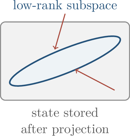
2.0.13 Modern Optimizer Frontier↩︎
Modern optimizer work revisits the same questions under large-model constraints. How much curvature can be exploited cheaply? How much optimizer state is necessary? Can a schedule be absorbed into the optimizer? Can matrix structure beat diagonal adaptivity at scale?
These questions are empirical and theoretical at the same time. A method can look attractive because it reduces memory, because it improves loss per token, because it improves wall-clock time, or because it reduces tuning effort. Those criteria need not agree. The theory problem is therefore not only to prove convergence in an idealized setting, but also to identify which algorithmic statistic is responsible for the observed gain.
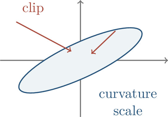
Sophia, or Second-order Clipped Stochastic Optimization, uses a lightweight diagonal Hessian or curvature estimate. Its goal is not full Newton training; it is to capture enough curvature information to prevent overly aggressive directions in language-model pretraining.
Sophia illustrates a recurring compromise in modern optimizers. Full second-order methods are too expensive at large scale, but purely diagonal gradient statistics may miss curvature. A cheap curvature proxy, combined with clipping, attempts to keep the update in a trust-region-like range without storing or inverting a full Hessian.
Lion is a different kind of simplification. In a simplified form, \[\theta_{t+1} = \theta_t - \eta\,\operatorname{sgn}(\beta m_t+(1-\beta)g_t).\] It uses signs rather than magnitudes for the update, compressing magnitude information and reducing optimizer state relative to Adam.
Sign-based updates separate direction from magnitude in an extreme way. The optimizer trusts the sign of a momentum-like direction but discards much of the coordinate-wise scale. This can make the method simple and memory efficient, but it also means that the learning-rate schedule and momentum state must carry more responsibility for controlling update size.
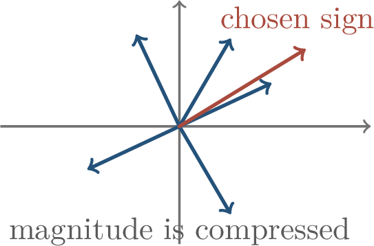
Learning-rate schedules are another major part of modern training. A schedule-free optimizer attempts to make schedule behavior internal to the algorithmic state.
This does not remove the need for hyperparameter choices; it changes where the choices live. Instead of prescribing a long hand-designed decay curve, the optimizer maintains averaged iterates or internal state intended to mimic the benefits of scheduling. The appeal is reduced tuning burden, especially when the same optimizer is reused across scales.
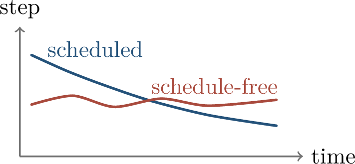
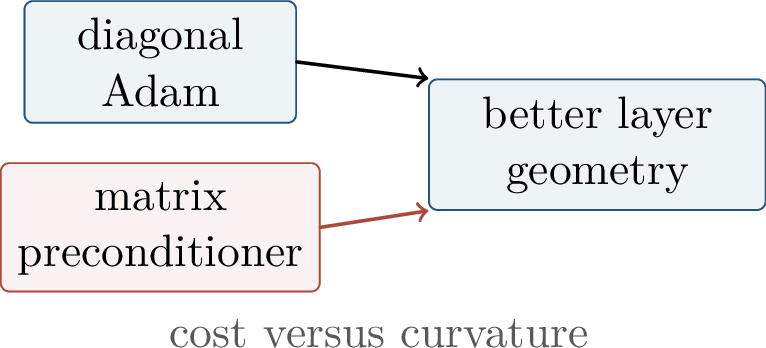
Long-memory momentum methods combine a fast memory with a slow memory: \[m_t^{\mathrm{fast}} = \beta_f m_{t-1}^{\mathrm{fast}}+(1-\beta_f)g_t, \qquad m_t^{\mathrm{slow}} = \beta_s m_{t-1}^{\mathrm{slow}}+(1-\beta_s)g_t.\] The fast component reacts to local changes, while the slow component stabilizes across long horizons.
This design reflects the fact that stochastic gradients contain information at multiple time scales. A short memory adapts quickly when the local geometry changes; a long memory preserves a stable direction across many noisy updates. Combining them is a way to avoid choosing a single exponential time constant for all phases of training.
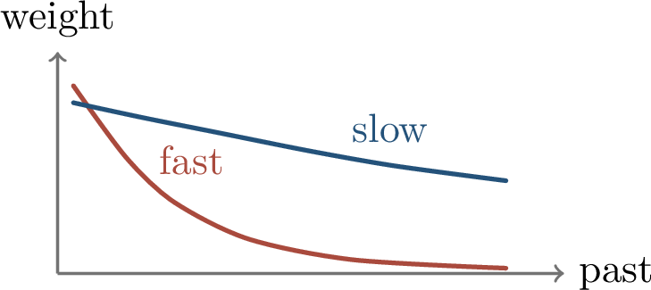
Finally, benchmarking optimizers is hard. A new optimizer may win because it received more tuning, because a small-scale proxy did not reflect large-scale behavior, or because wall-clock time, tokens, memory, and final loss point in different directions.
For a fair comparison, the unit of cost must be specified. Some methods reduce steps to a target loss but increase per-step cost. Some reduce memory but require more tuning. Some improve small models but fail to scale. A serious optimizer claim should therefore report the tuning protocol, compute budget, memory footprint, batch size, schedule choices, and scaling regime.
2.0.14 Synthesis↩︎
The conceptual map is now clear. SGD supplies the baseline Euclidean geometry. AdaGrad makes coordinate geometry data-dependent. AdamW adds exponential memory and separates weight decay from adaptive scaling. At foundation-model scale, memory and communication become first-class theoretical constraints, leading to factored, low-rank, sign-based, schedule-free, second-order, and matrix-preconditioned variants.
The unifying mathematical object is the preconditioner \(P_t\). In SGD it is the identity. In AdaGrad it is a diagonal matrix determined by accumulated squared gradients. In Adam and AdamW it is a diagonal matrix with exponential memory. In matrix and low-rank methods it is a structured approximation to a richer geometry. The practical differences between optimizers can therefore be read as different compromises among statistical adaptivity, invariance, memory, and compute.
First, adaptivity chooses a geometry: AdaGrad and Adam are data-dependent preconditioners, not merely faster SGD variants. Second, AdamW separates two effects: the adaptive gradient path and the weight-decay path. Third, scale changes the question: for foundation models, optimizer memory, communication, and tuning stability are part of the theory problem.
Important open questions include: when does AdamW generalize better or worse than SGD; what invariance principle is appropriate for scale-normalized networks; whether matrix preconditioners can beat AdamW after fair tuning at LLM scale; how much optimizer state is truly necessary for pretraining; and which benchmarks separate real optimization improvement from schedule or tuning effects.
Chapter Synthesis Adaptive optimization changes the geometry of descent. AdaGrad gives a clean regret-based view of data-dependent coordinate scaling. Adam replaces AdaGrad’s infinite memory with exponential first- and second-moment estimates. AMSGrad repairs a convergence pathology by enforcing a monotone denominator. AdamW decouples weight decay from adaptive normalization. Modern optimizer variants revisit these ideas under foundation-model memory, compute, and tuning constraints.
Core sources include AdaGrad by Duchi, Hazan, and Singer [30]; Adam by Kingma and Ba [31]; the marginal-value critique of adaptive methods by Wilson et al. [34]; the AMSGrad convergence repair of Reddi, Kale, and Kumar [32]; and AdamW by Loshchilov and Hutter [33]. For modern memory-efficient and large-model variants, see Shazeer and Stern, Adafactor: Adaptive Learning Rates with Sublinear Memory Cost; Chen et al., Symbolic Discovery of Optimization Algorithms; Liu et al., Sophia: A Scalable Stochastic Second-order Optimizer for Language Model Pre-training; Zhao et al., GaLore: Memory-Efficient LLM Training by Gradient Low-Rank Projection; Defazio et al., The Road Less Scheduled; Zhang et al., Adam-mini: Use Fewer Learning Rates To Gain More; and Pagliardini et al., The AdEMAMix Optimizer.
2.0.15 The Question of Selection↩︎
The previous chapter explained a mechanism by which sufficiently wide networks can reach zero training error. Reaching interpolation, however, is not the end of the story. Modern models are often so overparameterized that many parameter vectors have exactly the same empirical loss. Once the training error is zero, the empirical objective alone no longer distinguishes among the solutions.
This is where optimization becomes statistical again. If every interpolating solution were equivalent on future data, then the optimizer’s endpoint would not matter once the training loss reached zero. In practice, different interpolants can have very different norms, margins, sparsity patterns, ranks, and test behavior. The training algorithm therefore supplies information not visible in the empirical loss value. It selects a point by the geometry of the path it follows.
Definition 0.10 (Implicit regularization). Implicit regularization is the preference over solutions induced by the training algorithm, the initialization, the parameterization, and the training path, even when no explicit regularization penalty is added to the objective.
The guiding question for this chapter is therefore:
\[\textit{Among all zero-error solutions, which one does gradient descent find?}\]
This is a statistical question disguised as an optimization question. If different interpolating predictors generalize differently, then the path taken by the optimizer is part of the learning rule. The figures in this chapter are adapted from the Chapter 4 slides and serve as a running geometric language for this selection phenomenon.
The phrase “implicit regularization” should not be read as a guarantee of good generalization. It means that the algorithm behaves as if it preferred some solutions over others. Whether that preference is beneficial depends on the data distribution and architecture. The aim of this chapter is to compute the preference exactly in several simple models, and to use those computations as a guide for thinking about neural networks.
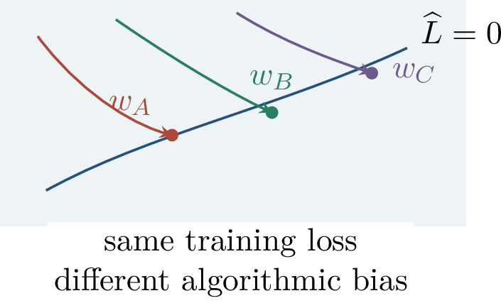
The chapter develops a three-step story. A parameterization \(w=g(\theta)\) changes the coordinates in which gradient descent is run. Those coordinates induce a geometry in the original \(w\)-space. Once the loss is driven to zero, that geometry often identifies the interpolant that is reached.
This viewpoint follows the optimization-geometry perspective of implicit bias: for underdetermined linear prediction and separable classification, the selected solution can often be described by a norm, potential, or Bregman divergence associated with the optimizer and parameterization [11], [12]. The least-squares examples below are deliberately elementary so that the geometry can be seen without the technical complications of deep networks.
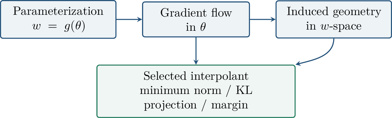
2.0.16 The Running Least-Squares Model↩︎
The cleanest model in which to see implicit regularization is an underdetermined least-squares problem. Let \[f(x)=\frac{1}{2}\left\lVert Ax-b \right\rVert_2^2, \qquad A\in\R^{n\times m},\qquad n<m.\] We assume throughout this section that the equations are consistent. Thus the interpolation set \[\mathcal{S}=\{x\in\R^m:Ax=b\}\] is nonempty and typically contains infinitely many points. We will compare two ways to optimize the same training loss: \[\text{linear parameterization: } x\in\R^m, \qquad \text{square parameterization: } x=y^{\odot 2}\in\R^m_{\ge 0}.\] The loss surface as a function of \(x\) is unchanged, but the gradient path is not. This distinction is the main lesson of the chapter.
The consistency assumption isolates implicit bias from optimization failure. Because \(\mathcal{S}\neq\emptyset\), zero training error is attainable. The question is not whether interpolation exists, but which point of the affine set is selected. In this simple model, the answer can be computed exactly. Direct gradient flow in \(x\) selects an \(\ell_2\) object. Gradient flow in a different parameterization of \(x\) selects a different object, even though the loss as a function of \(x\) is the same.
2.0.16.1 Linear Coordinates and Minimum Norm
First run continuous-time gradient descent directly on \(x\): \[x(0)=0,\qquad \dot{x}(t)=-\nabla f(x(t))=-A^\top(Ax(t)-b).\] The null space \(\ker(A)\) and the row space \(\operatorname{span}(A^\top)\) are orthogonal. Since every velocity vector is in the row space and the initial point is the origin, the entire trajectory remains in the row space: \[\require{physics} x(t)=\int_0^t -A^\top(Ax(s)-b)\dd s \in \operatorname{span}(A^\top).\] Consequently, if the trajectory converges to a feasible point, the limit is the unique feasible point orthogonal to \(\ker(A)\), namely the orthogonal projection of the origin onto \(\mathcal{S}\).
The row-space argument is the whole proof idea. Gradient flow can only move in directions generated by the rows of \(A\). It never creates a component in \(\ker(A)\), because null-space directions do not change the residual \(Ax-b\). Among all feasible points, adding a null-space component only increases the Euclidean norm, so the row-space feasible point is the minimum norm solution.
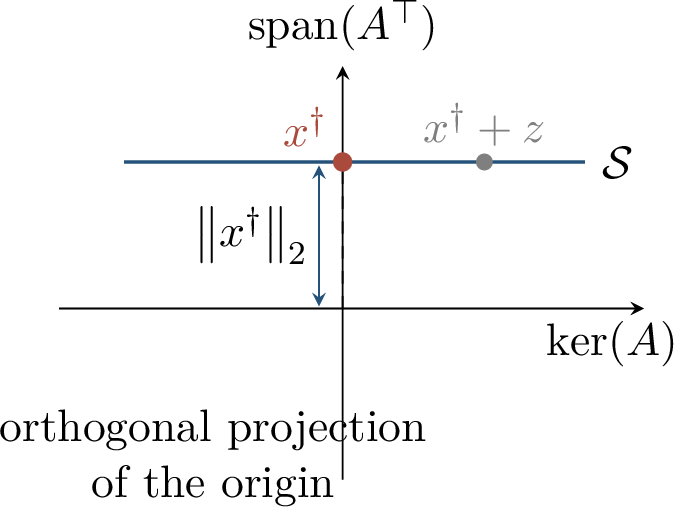
Lemma 0.4 (Minimum-norm bias of gradient flow). Assume \(Ax=b\) is consistent. Let \(x(0)=0\) and \[\dot{x}(t)=-A^\top(Ax(t)-b).\] If \(x(t)\) converges to a point in \(\mathcal{S}\), then \[x(t)\longrightarrow x^\dagger=\argmin_{Ax=b}\left\lVert x \right\rVert_2.\]
Proof. For every \(t\), the velocity \(\dot{x}(t)\) belongs to \(\operatorname{span}(A^\top)\). Since \(x(0)=0\), integration gives \[x(t)\in \operatorname{span}(A^\top) \quad \text{for all } t.\] Let \(x^\star\) be the assumed limit. Then \(Ax^\star=b\), and \(x^\star\in\operatorname{span}(A^\top)\). For any other feasible point \(x^\star+z\) with \(z\in\ker(A)\), orthogonality of the row and null spaces gives \[\left\lVert x^\star+z \right\rVert_2^2=\left\lVert x^\star \right\rVert_2^2+\left\lVert z \right\rVert_2^2.\] Thus \(x^\star\) is the closest feasible point to the origin. ◻
The reference notes emphasize that convergence to a feasible point is an assumption in this lemma; the selection statement is conditional on interpolation. This is typical in implicit-bias results. The theorem characterizes what is reached, not always whether training reaches it.
For this linear least-squares flow, convergence can also be checked directly under mild rank conditions. The residual \(r(t)=Ax(t)-b\) satisfies \[\dot{r}(t)=-AA^\top r(t),\] so all residual components in the range of \(A\) decay exponentially. The chapter keeps the lemma in conditional form because later examples, especially nonlinear and neural-network examples, require more care: optimization and selection are logically distinct.
For \(\lambda>0\), let \[x_\lambda = \argmin_x \left\{ \frac{1}{2}\left\lVert Ax-b \right\rVert_2^2 +\frac{\lambda}{2}\left\lVert x \right\rVert_2^2 \right\}.\] If \(Ax=b\) is consistent, then \[x_\lambda\to x^\dagger \qquad \text{as } \lambda\downarrow 0.\]
Proof. The ridge solution is \[x_\lambda=(A^\top A+\lambda I)^{-1}A^\top b =A^\top(AA^\top+\lambda I)^{-1}b.\] As \(\lambda\downarrow0\), this converges to \(A^\top(AA^\top)^\dagger b\), the Moore-Penrose minimum-norm solution of \(Ax=b\). Equivalently, ridge regression shrinks toward the origin and, in the vanishing-penalty limit, keeps the closest interpolant. ◻
The vanishing ridge result provides a useful comparison between explicit and implicit regularization. Explicit ridge regression adds the penalty \(\lambda\left\lVert x \right\rVert_2^2/2\) and then takes \(\lambda\) small. Gradient flow from the origin adds no such penalty to the objective, yet it selects the same minimum-\(\ell_2\) interpolant. In this example the implicit bias of the algorithm is exactly mirrored by an explicit regularizer.
Explicit Proxy for an Implicit Bias Direct least-squares gradient flow from \(0\) selects the same interpolant as vanishing ridge regularization: the minimum Euclidean-norm solution of \(Ax=b\). This equivalence is special to the linear Euclidean setting; later parameterizations lead to different explicit proxies.
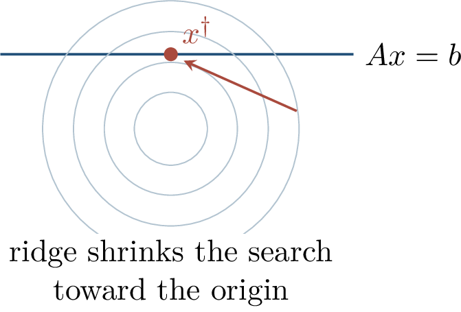
2.0.17 Reparameterization Changes the Bias↩︎
Now reparameterize the same least-squares problem by the entrywise square map \[x=\operatorname{sq}(y)=y^{\odot 2}, \qquad \widehat f(y)=\frac{1}{2}\left\lVert A\,y^{\odot 2}-b \right\rVert_2^2.\] The variable \(x\) is now restricted to the nonnegative orthant. More importantly, Euclidean gradient flow in \(y\) induces a non-Euclidean flow in \(x\).
This example is intentionally minimal. The feasible set in \(x\)-space is still defined by the same linear equations \(Ax=b\), but the optimizer no longer moves with the Euclidean metric in \(x\). A small value of \(x_i\) corresponds to a small value of \(y_i\), and the chain rule makes the induced \(x_i\)-velocity proportional to \(x_i\). Coordinates near zero are therefore sticky. This stickiness is the dynamical origin of sparsity.
Let \(x(t)=y(t)^{\odot 2}\), \(D_y=\diag(y(t))\), and \(D_x=\diag(x(t))\). If \[\dot{y}(t)=-\nabla_y\widehat f(y(t)),\] then \[\dot{y}(t)=-2D_yA^\top(Ax(t)-b), \qquad \dot{x}(t)=-4D_xA^\top(Ax(t)-b).\]
Proof. By the chain rule, the Jacobian of \(y\mapsto y^{\odot2}\) is \(2D_y\), so \[\nabla_y\widehat f(y)=2D_yA^\top(Ay^{\odot2}-b).\] Differentiating \(x_i(t)=y_i(t)^2\) gives \[\dot{x}(t)=2D_y\dot{y}(t) =-4D_y^2A^\top(Ax(t)-b) =-4D_xA^\top(Ax(t)-b).\] ◻
The diagonal factor \(D_x\) changes the local geometry. Coordinates with small \(x_i\) move slowly; positive coordinates remain positive in the continuous flow. The reference notes phrase this as the basic proof outline: study mirror descent, interpret the reparameterized gradient flow as mirror flow, and then identify the limiting Bregman projection.
One can read the equation \[\dot{x}(t)=-4D_xA^\top(Ax(t)-b)\] as a preconditioned flow. The preconditioner \(D_x\) is not chosen by hand; it is induced by the square parameterization. This is why implicit regularization is sensitive to coordinates. Euclidean gradient descent in one parameter space may become mirror descent in another.
Theorem 0.4 (Small-initialization \(\ell_1\) bias). Suppose the square-parameterized gradient flow converges to a zero-error point \(x^\star(\alpha)\) from a positive initialization with \(x(0)=\alpha\mathbf{1}\). Under the standard regularity conditions that justify the Bregman-projection limit, every limit point as \(\alpha\downarrow0\) solves \[\min_{\substack{x\ge0\\Ax=b}}\left\lVert x \right\rVert_1.\] In the common case where this minimizer is unique, \[x^\star(\alpha)\longrightarrow \argmin_{\substack{x\ge0\\Ax=b}}\left\lVert x \right\rVert_1.\]
This is the main surprise of the chapter. Direct optimization in \(x\) selects the minimum \(\ell_2\)-norm interpolant, while Euclidean optimization in the square root coordinates \(y\) selects a nonnegative minimum-\(\ell_1\) interpolant at small initialization. The feasible equations are the same; only the parameterization changes.
The small-initialization limit is essential. For fixed positive \(\alpha\), the entropy/KL geometry still remembers the initialization \(\alpha\mathbf{1}\). As \(\alpha\downarrow0\), the dominant part of the Bregman projection becomes proportional to \(\left\lVert x \right\rVert_1\), so the selected solution approaches the nonnegative basis-pursuit solution. Thus the theorem links three objects: the square parameterization, entropy mirror geometry, and \(\ell_1\) sparsity.
Why Sparsity Appears The square map makes coordinates near zero hard to move. Entropy mirror geometry formalizes this effect, and the small positive initialization turns the corresponding Bregman projection into an \(\ell_1\)-minimization problem.
2.0.17.1 Norm Geometry and Sparsity
The difference between \(\ell_2\) and \(\ell_1\) selection is visible in the geometry of norm balls. An \(\ell_2\) ball is round, so its first contact with an affine constraint tends to occur at a dense point. An \(\ell_1\) ball has corners aligned with coordinate axes, and first contact often occurs at a sparse point.
This geometric explanation is not a proof of compressed sensing, but it gives the correct intuition. Linear constraints define an affine slice. Minimizing a norm asks which scaled norm ball first touches that slice. Corners of the \(\ell_1\) ball make axis-aligned contact likely, and axis-aligned contact means some coordinates are zero.
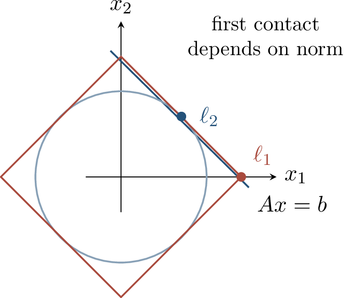
Example 0.2 (Basis pursuit and compressed sensing). The convex program \[\min_x \left\lVert x \right\rVert_1 \quad \text{subject to}\quad Ax=b\] is called basis pursuit. It is central in compressed sensing because, for many random sensing matrices, a \(k\)-sparse vector in \(\R^m\) can be recovered from on the order of \[k\log(m/k)\] random linear measurements. Thus the square parameterization is not merely a toy: it links gradient-flow bias to an algorithmic principle for sparse recovery.
The compressed-sensing statement requires assumptions on \(A\), such as restricted isometry or related incoherence conditions. Without such conditions, \(\ell_1\) minimization can fail to recover the sparsest solution. For this chapter, the important point is more modest: the same implicit \(\ell_1\) bias induced by square-root parameterization is the explicit bias that underlies basis pursuit.
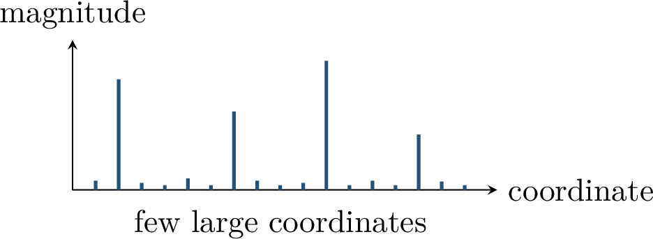
Example 0.3 (A two-dimensional toy problem). Let \[A=\begin{bmatrix}1&2\end{bmatrix}, \qquad b=1,\qquad x\ge0.\] The feasible set is the line segment \(x_1+2x_2=1\). Direct computation gives \[\argmin_{Ax=b}\left\lVert x \right\rVert_2 = \left(\frac{1}{5},\frac{2}{5}\right), \qquad \argmin_{\substack{Ax=b\\x\ge0}}\left\lVert x \right\rVert_1 = \left(0,\frac{1}{2}\right).\] The \(\ell_1\) solution is sparser because it lies on a coordinate axis.
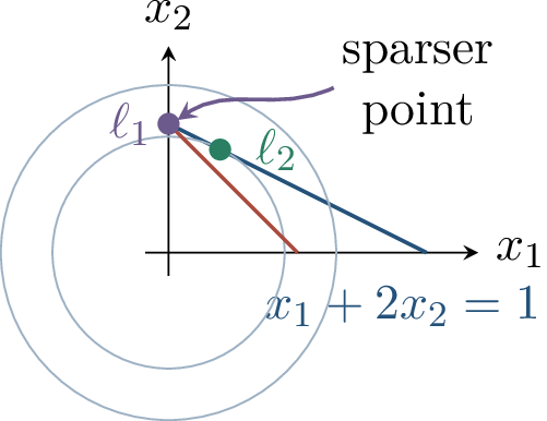
2.0.18 Mirror Descent and Bregman Geometry↩︎
We now introduce the geometry that explains the preceding phenomenon. Standard gradient descent can be written as a proximal step: \[x_{t+1} = \argmin_x \left\{ f(x_t)+\left\langle \nabla f(x_t),x-x_t \right\rangle +\frac{1}{2\eta}\left\lVert x-x_t \right\rVert_2^2 \right\}.\] That is, minimize the linear approximation of \(f\) at \(x_t\), but do not move too far in Euclidean distance. Mirror descent replaces the Euclidean distance with a divergence adapted to the problem geometry.
The proximal form is useful because it separates two roles of the algorithm. The linear term says which direction decreases the objective at the current point. The quadratic term says which movements are considered cheap. Ordinary gradient descent regards a unit movement in each coordinate as equally costly. Mirror descent changes this notion of cost. Coordinates near the boundary, coordinates with large curvature, or coordinates with different physical meaning can be treated differently through the choice of \(\phi\).
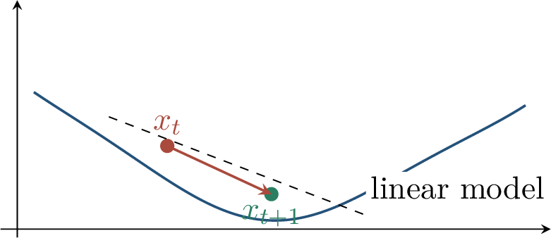
Definition 0.11 (Bregman divergence). Let \(\phi:\R^m\to\R\) be differentiable and strictly convex on a convex domain. The Bregman divergence generated by \(\phi\) is \[D_\phi(x,z) = \phi(x)-\phi(z)-\left\langle \nabla\phi(z),x-z \right\rangle.\]
The quantity \(D_\phi(x,z)\) is the error made by the first-order Taylor approximation of \(\phi\) at \(z\) when evaluated at \(x\). It is nonnegative, but it is not usually symmetric and need not satisfy the triangle inequality. Locally, when \(\phi\) is twice differentiable, \[D_\phi(x,z)\approx \frac{1}{2}(x-z)^\top \nabla^2\phi(z)(x-z).\] Thus the Hessian of \(\phi\) chooses a local metric.
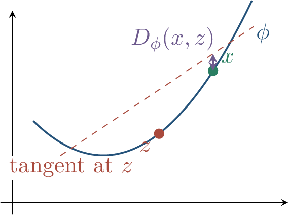
Definition 0.12 (Mirror descent). Given a differentiable strictly convex mirror map \(\phi\), mirror descent with stepsize \(\eta>0\) updates by \[x_{t+1} = \argmin_x \left\{ f(x_t)+\left\langle \nabla f(x_t),x-x_t \right\rangle +\frac{1}{\eta} D_\phi(x,x_t) \right\}.\]
Lemma 0.5 (Dual-space update). If the mirror descent subproblem is solved at an interior point, then \[\nabla\phi(x_{t+1})-\nabla\phi(x_t) = -\eta\nabla f(x_t).\]
Proof. Differentiate the mirror descent objective with respect to \(x\) and set the gradient equal to zero at \(x=x_{t+1}\): \[\nabla f(x_t) +\frac{1}{\eta}\bigl(\nabla\phi(x_{t+1})-\nabla\phi(x_t)\bigr)=0.\] Rearranging gives the claim. ◻
The Euclidean mirror map \(\phi(x)=\frac{1}{2}\left\lVert x \right\rVert_2^2\) recovers ordinary gradient descent. The entropy mirror map on the positive orthant, \[\phi(x)=\sum_i x_i\log x_i-\sum_i x_i,\] has \[\nabla^2\phi(x)=\diag(1/x_i)\] and Bregman divergence \[D_\phi(x,z) = \sum_i x_i\log\frac{x_i}{z_i} -\sum_i x_i+\sum_i z_i.\] The boundary \(x_i=0\) is infinitely far in this local metric. In discrete time, the update has a multiplicative form, \[x_{t+1,i}=x_{t,i}\exp\!\bigl(-\eta[\nabla f(x_t)]_i\bigr),\] so positive iterates remain positive.
This is exactly the qualitative behavior seen in the square parameterization. Small coordinates move slowly because the induced metric makes relative changes natural and absolute changes expensive. Thus the geometry carries information about sparsity: coordinates that start close to zero are not easily activated unless the loss gradient keeps pushing them.
2.0.19 Bregman Projection as Implicit Bias↩︎
For least squares, mirror descent does not merely converge to some feasible point; when it converges to interpolation, it reaches the Bregman projection of the initialization onto the feasible set.
This statement generalizes the minimum-\(\ell_2\) result from the first part of the chapter. With the Euclidean mirror map, \(D_\phi(x,x_1)\) is just \(\frac{1}{2}\left\lVert x-x_1 \right\rVert_2^2\), so the limit is the closest feasible point to the initialization in Euclidean distance. With entropy, closeness is measured by a KL-type divergence, and the projection becomes compatible with nonnegative sparse solutions.
Theorem 0.5 (Bregman projection bias). Let \(f(x)=\frac{1}{2}\left\lVert Ax-b \right\rVert_2^2\). Suppose mirror descent initialized at \(x_1\) converges to a feasible point and that the stepsizes are chosen so that the usual convergence argument applies. Then \[x_t\longrightarrow \argmin_{Ax=b} D_\phi(x,x_1).\]
Proof sketch. Let \(g_t=\nabla\phi(x_t)\). The dual update gives \[\begin{align} g^\star-g_1 &=\sum_{t\ge1}(g_{t+1}-g_t) \\ &= -\sum_{t\ge1}\eta_t A^\top(Ax_t-b) \in \operatorname{span}(A^\top), \end{align}\] where \(g^\star=\nabla\phi(x^\star)\) and \(x^\star\) is the limit. On the other hand, \[\nabla_x D_\phi(x,x_1)\big|_{x=x^\star} = \nabla\phi(x^\star)-\nabla\phi(x_1) =g^\star-g_1.\] Thus the gradient of the objective \(D_\phi(\cdot,x_1)\) at the limit lies in the row space of \(A\), which is the normal space to the affine constraint set \(\{x:Ax=b\}\). This is the KKT condition for minimizing \(D_\phi(x,x_1)\) over \(Ax=b\). Convexity of \(D_\phi(\cdot,x_1)\) in its first argument completes the projection argument. ◻
The proof is a KKT argument written in the language of dynamics. The optimization path keeps track of the cumulative gradients, and for least squares every gradient lies in the row space of \(A\). At convergence, this cumulative row-space vector is exactly the gradient of the Bregman divergence from the initialization. Therefore the endpoint satisfies the first-order optimality condition for a constrained projection problem.
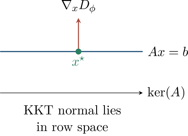
2.0.19.1 Square Flow as Entropy Mirror Flow
For the entropy mirror map, \[\nabla^2\phi(x)=D_x^{-1}.\] The continuous-time mirror flow associated with \(f\) is \[\dot{x}(t)=-(\nabla^2\phi(x(t)))^{-1}\nabla f(x(t)).\] For least squares this becomes \[\dot{x}(t)=-D_xA^\top(Ax(t)-b).\] Comparing with the square-parameterized flow \[\dot{x}(t)=-4D_xA^\top(Ax(t)-b),\] we see that the two are identical up to the constant time rescaling by \(4\). Thus the square map turns Euclidean gradient flow in \(y\) into entropy mirror flow in \(x\).
The constant \(4\) has no effect on the limiting interpolant in continuous time; it only changes the speed at which the trajectory is traversed. The important object is the matrix \(D_x\). It says that the effective learning rate of coordinate \(i\) is proportional to \(x_i\), which is the continuous analogue of multiplicative weights.
Lemma 0.6 (KL projection limit). For entropy \(\phi(x)=\sum_i x_i\log x_i-\sum_i x_i\) and initialization \(x_1=\alpha\mathbf{1}\), \[D_\phi(x,\alpha\mathbf{1}) = \sum_i x_i\log x_i +\left(\log\frac{1}{\alpha}-1\right)\left\lVert x \right\rVert_1 +\alpha m .\]
Proof. Using the entropy Bregman divergence, \[D_\phi(x,\alpha\mathbf{1}) = \sum_i x_i\log\frac{x_i}{\alpha} -\sum_i x_i+\sum_i \alpha.\] Expanding the logarithm gives the displayed formula. ◻
As \(\alpha\downarrow0\), the coefficient \(\log(1/\alpha)-1\) diverges. On bounded feasible sets, the entropy term \(\sum_i x_i\log x_i\) is lower order relative to this coefficient. Therefore minimizers of \[\min_{\substack{x\ge0\\Ax=b}}D_\phi(x,\alpha\mathbf{1})\] approach minimizers of \[\min_{\substack{x\ge0\\Ax=b}}\left\lVert x \right\rVert_1.\] The reference notes caution that one must handle the order of limits carefully: for each fixed \(\alpha\), the flow converges to an approximate KL projection, and the approximation gap vanishes as \(\alpha\to0\).
The order of limits is not a cosmetic issue. If the initialization is fixed away from zero, the entropy term can still influence the selected feasible point. The \(\ell_1\) statement is obtained by first identifying the Bregman-projection limit for a fixed positive initialization and then studying what happens as that initialization tends to the boundary of the positive orthant.
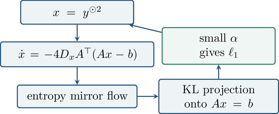
2.0.20 Connections to Deep Learning↩︎
Neural networks are highly reparameterized models. Layers can be scaled against each other, features are shared across examples, and many architectures are homogeneous. The lesson of the square map is therefore broader than least squares: changing coordinates can change the geometry seen by the optimizer, and that geometry can encode a norm, a margin, a low-rank preference, or a more subtle architecture-dependent bias.
This does not mean that every neural network secretly minimizes a simple closed-form norm. The examples in this chapter should instead be read as calibrated test cases. In each case the loss alone leaves many interpolants, and the training dynamics supplies an additional variational principle. The principle may be Euclidean projection, entropy projection, maximum margin, or a matrix-geometric preference, depending on the model.
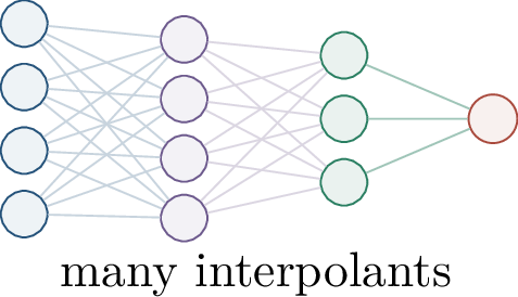
2.0.20.1 Linear Classification and Maximum Margin
A second canonical example concerns separable linear classification. Consider data \(\{(x_i,y_i)\}_{i=1}^N\) with \(y_i\in\{\pm1\}\). The data are linearly separable if there exists a vector \(a\) (and, if desired, an intercept that can be absorbed into the features) such that \[\operatorname{sign}(a^\top x_i)=y_i \quad \text{for all } i.\] Among all separators, a maximum-margin separator keeps the examples farthest from the decision boundary after normalizing \(\left\lVert a \right\rVert_2=1\).
Theorem 0.6 (Implicit bias for separable data). For linearly separable data and losses with exponential tails, such as \[L(a)=\sum_i \exp(-y_i a^\top x_i),\] gradient descent or gradient flow drives \(\left\lVert a(t) \right\rVert_2\to\infty\), but the direction converges: \[\frac{a(t)}{\left\lVert a(t) \right\rVert_2} \longrightarrow \frac{a^\star}{\left\lVert a^\star \right\rVert_2},\] where \(a^\star\) is the hard-margin SVM solution. More precisely, the asymptotic growth has the form \[a(t)=a^\star\log t+O(\log\log t)\] in the separable exponential-loss setting.
This result is another implicit-regularization statement. The empirical loss does not attain a finite minimizer on separable data; the norm diverges. Yet the direction of the classifier converges to a geometrically distinguished solution, the maximum-margin separator [11].
The distinction between scale and direction is essential. Multiplying a separator by a large positive constant makes the exponential loss smaller, but it does not change the classifier. Thus the optimizer spends late training time increasing the norm while slowly rotating the direction toward the hard-margin solution. The limiting predictor is therefore best described after normalization, not by the parameter vector itself.
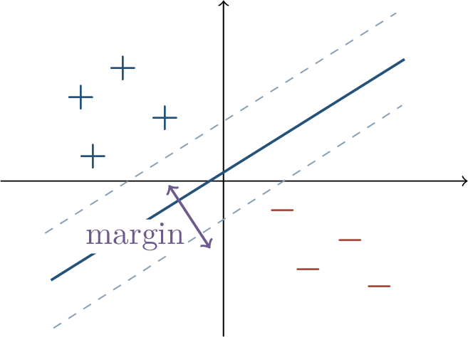
The reference notes also mention the generalization-bound motivation: classical margin bounds for support vector machines suggest that large margin can be statistically meaningful. The subtle question is whether maximizing such a bound is the same as maximizing real test performance. The theory gives an important clue, not a complete explanation of generalization.
In this sense, maximum margin plays the same role for separable classification that minimum norm played for linear regression: it identifies a particular solution among infinitely many zero-training-error predictors. The selected quantity is different because the loss landscape is different. Regression has a finite affine solution set; separable classification has no finite minimizer, so the meaningful object is the asymptotic direction.
2.0.20.2 Matrix Factorization and Low Rank
Matrix factorization provides a third example. In positive semidefinite sensing one writes \[X=YY^\top, \qquad \min_Y \sum_i \bigl(\mathcal{L}_i(YY^\top)-b_i\bigr)^2.\] The variable being trained is \(Y\), while the prediction is expressed through the matrix \(X=YY^\top\). This is the matrix analogue of the scalar square map: the feasible set is described in \(X\)-space, but gradient flow is run in a factor space. The factorization automatically enforces \(X\succeq0\) and creates a non-Euclidean geometry on positive semidefinite matrices.
Because the nuclear norm of a positive semidefinite matrix is its trace, it was natural to conjecture that gradient flow might prefer \[\argmin_{\substack{X\succeq0\\ \mathcal{L}_i(X)=b_i}} \left\lVert X \right\rVert_\ast .\] The diagonal case reduces to the square-parameterized \(\ell_1\) story: diagonal PSD matrices correspond to nonnegative vectors, and the nuclear norm becomes the \(\ell_1\) norm of the diagonal.
The full noncommutative case is more delicate. Under matrix RIP assumptions, related low-rank recovery statements hold, but the clean universal nuclear-norm conjecture is false in full generality: some results show that gradient flow may find an even lower-rank solution rather than exactly the nuclear-norm minimizer. This is an important warning. Even in simple matrix models, the implicit regularizer can be subtler than the most natural convex norm [12].
One reason is that matrices do not commute. In the diagonal case, each coordinate evolves independently and the entropy picture almost literally reduces to the vector \(\ell_1\) story. For general matrices, eigenvectors can rotate, singular subspaces can interact, and the factor \(Y\) contains symmetries that are invisible in \(X\). The induced geometry therefore cannot always be summarized by replacing \(\ell_1\) with the nuclear norm.
| Model or update | Geometry | Selected solution |
|---|---|---|
| \(x\) directly | Euclidean | minimum \(\ell_2\) norm |
| \(x=y^{\odot2}\) | entropy / KL | nonnegative minimum \(\ell_1\) |
| \(X=YY^\top\) | matrix factor geometry | low-rank bias |
| separable linear model | exponential-tail flow | maximum margin |
| homogeneous networks | scale-invariant paths | norm or margin bias |
2.0.21 Limitations and Open Questions↩︎
Implicit regularization is powerful because it explains why interpolation does not make all solutions equivalent. Still, the chapter emphasizes several caveats.
First, many statements assume convergence to an interpolating solution. The selection theorem is then conditional: if the dynamics reaches zero training error, it characterizes which zero-error point is reached. Second, entropy geometry is singular at the boundary of the positive orthant, and the order of limits in time, stepsize, and initialization can matter. Third, stochasticity, finite step sizes, momentum, and adaptive optimizers can change the path. A continuous-time mirror-flow analysis may be the right idealization for one regime and the wrong one for another.
In neural networks, additional complications enter. Real architectures are nonlinear and nonconvex; the relevant implicit bias may depend on depth, homogeneity, normalization, data geometry, and the optimizer. A norm or margin bound may correlate with generalization in some settings without fully explaining test accuracy. The open direction is to find implicit regularizers that are predictive, architecture-aware, and robust to training details.
Chapter Synthesis This chapter developed implicit regularization as a selection principle. In underdetermined least squares, Euclidean gradient flow from the origin selects the minimum-\(\ell_2\) interpolant. Under the square parameterization \(x=y^{\odot2}\), the induced flow becomes an entropy mirror flow and, from small positive initialization, approaches a nonnegative minimum-\(\ell_1\) interpolant. Mirror descent unifies these examples through Bregman projection. The same logic also explains why separable exponential-loss classification selects a maximum-margin direction and why matrix factorization exhibits a low-rank, geometry-dependent bias. The central lesson is that interpolation is not a single endpoint; it is a set, and optimization chooses a point in that set.
Core references for this chapter include the optimization-geometry viewpoint of Gunasekar, Lee, Soudry, and Srebro [12] and the maximum-margin analysis of Soudry, Hoffer, Nacson, Gunasekar, and Srebro [11]. For standard background on margins, empirical risk minimization, and support vector machines, see Shalev-Shwartz and Ben-David [2]. The selected literature also points to Moitra’s and Telgarsky’s deep learning theory chapters for broader context, and to the classical mirror-descent and compressed-sensing literature for the convex optimization ideas used here.
3 Generalization, Stability, and Complexity↩︎
3.0.1 From Fitting to Generalization↩︎
The preceding chapters focused on the fitting side of deep learning: expressive models, interpolation, optimization, and the implicit biases of training algorithms. These ideas answer questions of the form “can the model drive the training loss to zero?” and “which interpolating solution does the optimizer select?” They do not by themselves answer the statistical question that makes learning meaningful: will a predictor that fits the training data also perform well on new examples drawn from the same distribution?
This chapter studies classical and modern ways to control the gap between training performance and population performance. The central quantity is \[\sup_{h\in\mathcal{H}} \left\lvert \operatorname{err}_\mathcal{D}(h)-\operatorname{err}_S(h) \right\rvert ,\] where \(S\) is the observed sample, \(\mathcal{D}\) is the unknown data distribution, and \(\mathcal{H}\) is a hypothesis class. A useful generalization bound trades among three quantities: the sample size \(N\), the complexity of \(\mathcal{H}\), and the confidence level \(1-\delta\).
The supremum over \(h\in\mathcal{H}\) is the key point. If a single classifier is fixed before the data are drawn, concentration of independent random variables is enough. A learning algorithm, however, chooses its classifier after seeing the sample. The same sample is therefore used both to fit the model and to estimate its error. Uniform convergence asks for a statement strong enough to remain valid after this data-dependent choice has been made.
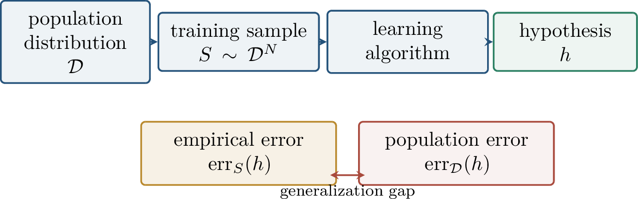
Definition 0.13 (Empirical and population error). Let \(S=\{(x_i,y_i)\}_{i=1}^N\) be drawn independently from a distribution \(\mathcal{D}\) on \(\R^d\times\{0,1\}\). For a binary classifier \(h:\R^d\to\{0,1\}\), define \[\operatorname{err}_S(h) = \frac{1}{N}\sum_{i=1}^N \mathbf{1}{h(x_i)\ne y_i}, \qquad \operatorname{err}_\mathcal{D}(h) = \Prob_{(x,y)\sim\mathcal{D}}\!\left[h(x)\ne y\right].\] The generalization gap on \(S\) is \[\operatorname{gap}_S(h) = \left\lvert \operatorname{err}_\mathcal{D}(h)-\operatorname{err}_S(h) \right\rvert .\]
When \(h\) is fixed before seeing the data, the empirical error is an average of independent Bernoulli variables and concentrates around its expectation. The difficulty is that learning chooses \(h\) after seeing \(S\). A generalization theorem must therefore control many hypotheses at once. The chapter develops three increasingly refined lenses.
Throughout this chapter the loss is the zero-one classification loss unless explicitly stated otherwise. This keeps the notation close to PAC learning and VC theory. The same philosophy extends to bounded real-valued losses, but the technical tools then use covering numbers, Rademacher complexity, or concentration inequalities for bounded random variables rather than only Bernoulli averages.
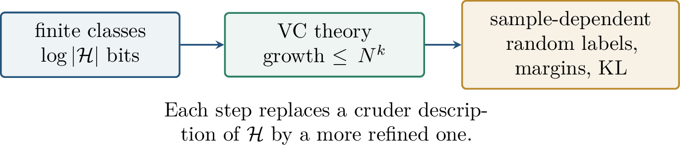
3.0.2 Finite Hypothesis Classes↩︎
The cleanest result is obtained when the hypothesis class is finite. This is not a realistic description of a neural network with real-valued weights, but it captures the main statistical mechanism: a class generalizes when it cannot encode too many independent label patterns relative to the sample size.
Lemma 0.7 (Hoeffding’s inequality for Bernoulli averages). Let \(X_1,\ldots,X_N\) be independent random variables taking values in \(\{0,1\}\), and let \(p=\E X_i\). Then for every \(\epsilon>0\), \[\Prob\left[ \left\lvert \frac{1}{N}\sum_{i=1}^N X_i-p \right\rvert\ge \epsilon \right] \le 2e^{-2N\epsilon^2}.\]
Theorem 0.7 (Finite-class uniform convergence). Let \(\mathcal{H}\) be a finite class of binary classifiers. For every \(\epsilon,\delta>0\), if \[N\ge \frac{1}{2\epsilon^2} \left( \log(2|\mathcal{H}|)+\log\frac{1}{\delta} \right),\] then, with probability at least \(1-\delta\) over \(S\sim\mathcal{D}^N\), \[\forall h\in\mathcal{H},\qquad \left\lvert \operatorname{err}_\mathcal{D}(h)-\operatorname{err}_S(h) \right\rvert\le \epsilon .\]
Proof. Fix \(h\in\mathcal{H}\). The variables \[X_i=\mathbf{1}{h(x_i)\ne y_i}\] are independent Bernoulli variables with mean \(\operatorname{err}_\mathcal{D}(h)\), and their average is \(\operatorname{err}_S(h)\). Hoeffding’s inequality gives \[\Prob\left[\left\lvert \operatorname{err}_\mathcal{D}(h)-\operatorname{err}_S(h) \right\rvert>\epsilon\right] \le 2e^{-2N\epsilon^2}.\] Taking a union bound over all \(h\in\mathcal{H}\), \[\Prob\left[ \exists h\in\mathcal{H}: \left\lvert \operatorname{err}_\mathcal{D}(h)-\operatorname{err}_S(h) \right\rvert>\epsilon \right] \le 2|\mathcal{H}|e^{-2N\epsilon^2}.\] The stated lower bound on \(N\) makes the final expression at most \(\delta\). ◻
Solving the same inequality for \(\epsilon\) gives the familiar form \[\sup_{h\in\mathcal{H}}\left\lvert \operatorname{err}_\mathcal{D}(h)-\operatorname{err}_S(h) \right\rvert \le \sqrt{ \frac{\log(2|\mathcal{H}|)+\log(1/\delta)}{2N} }\] with probability at least \(1-\delta\). The square-root dependence on \(1/N\) is typical for two-sided estimation: the empirical average fluctuates above and below its mean. The logarithm of \(|\mathcal{H}|\), rather than \(|\mathcal{H}|\) itself, is the price paid for searching over the class.
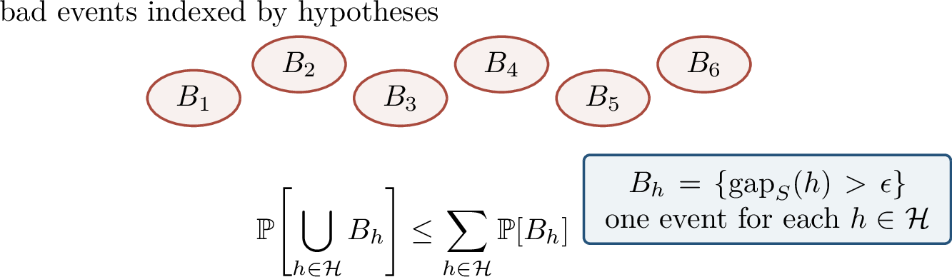
The theorem is agnostic: it makes no assumption that the labels are generated by a member of \(\mathcal{H}\). Under a realizability assumption one can obtain a faster \(1/N\) dependence in the error level.
Assume there exists \(h^\star\in\mathcal{H}\) such that \(y=h^\star(x)\) almost surely, and suppose an algorithm returns \(h\in\mathcal{H}\) with \(\operatorname{err}_S(h)=0\). Then, with probability at least \(1-\delta\), \[\operatorname{err}_\mathcal{D}(h) \le \frac{\log|\mathcal{H}|+\log(1/\delta)}{N}.\]
Proof. Fix a hypothesis \(h\) with population error larger than \(\epsilon\). Since examples are independent, the probability that all \(N\) training examples miss the error region of \(h\) is at most \[(1-\epsilon)^N\le e^{-\epsilon N}.\] Thus \[\Prob\!\left[ \exists h\in\mathcal{H}: \operatorname{err}_\mathcal{D}(h)>\epsilon \text{ and } \operatorname{err}_S(h)=0 \right] \le |\mathcal{H}|e^{-\epsilon N}.\] Set the right-hand side equal to \(\delta\) and solve for \(\epsilon\). ◻
The realizable bound has a different flavor from the previous theorem. It is not estimating the error of every hypothesis to accuracy \(\epsilon\); it is only ruling out the event that a bad hypothesis happens to make no mistakes on the sample. A classifier with true error \(\epsilon\) survives \(N\) independent examples with probability at most \(e^{-\epsilon N}\). This one-sided argument is why the rate is proportional to \(1/N\) in the error level, rather than \(1/\sqrt N\).
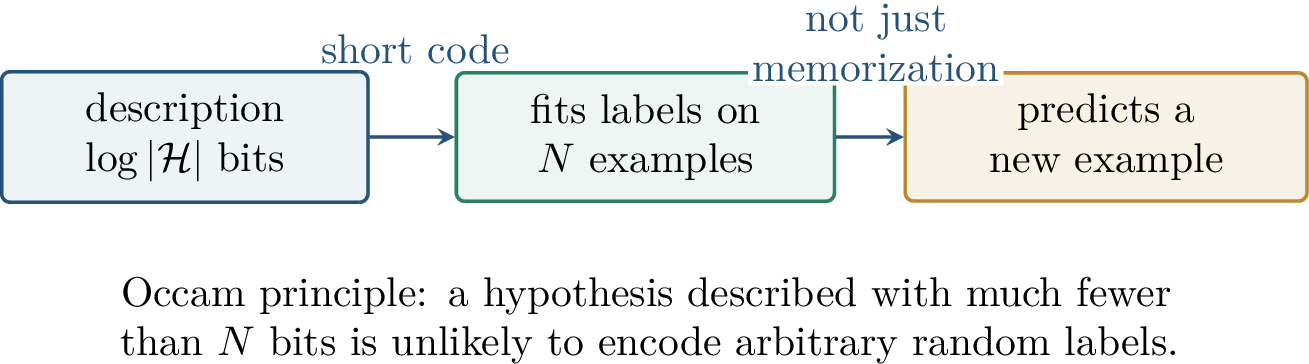
The factor \(\log|\mathcal{H}|\) is the description cost of selecting one member of the class. This is too crude for real-valued neural networks, but the principle survives throughout the chapter: better descriptions of the learned predictor lead to sharper generalization statements.
3.0.3 VC Dimension and Growth Functions↩︎
The finite-class theorem fails literally when \(|\mathcal{H}|=\infty\). VC theory replaces the number of hypotheses by the number of distinct labelings that \(\mathcal{H}\) can realize on finite samples. This shift is essential: an infinite class may behave like a polynomial-size class when restricted to \(N\) points. The development here follows the standard distribution-free learning theory viewpoint of Vapnik and of modern learning-theory texts [1], [2].
Definition 0.14 (Shattering and VC dimension). Let \(\mathcal{H}\) be a class of binary classifiers on \(\mathcal{X}\). A finite set \(T=\{x_1,\ldots,x_m\}\subset\mathcal{X}\) is shattered by \(\mathcal{H}\) if for every label vector \((y_1,\ldots,y_m)\in\{0,1\}^m\) there exists \(h\in\mathcal{H}\) such that \(h(x_i)=y_i\) for all \(i\). The VC dimension is \[\operatorname{VCdim}(\mathcal{H}) = \max\{m:\text{some }m\text{-point set is shattered by }\mathcal{H}\},\] with value \(+\infty\) if such sets exist for all \(m\).
The word “some” in the definition is important. To prove \(\operatorname{VCdim}(\mathcal{H})\ge m\), it is enough to exhibit one \(m\)-point configuration that can be shattered. To prove \(\operatorname{VCdim}(\mathcal{H})<m\), one must show that no \(m\)-point configuration can be shattered. Thus lower bounds are often constructive, while upper bounds usually require a combinatorial or geometric argument.

Example 0.4 (Halfspaces). Let \[\mathcal{H} = \left\{ x\mapsto \operatorname{sgn}(a^\top x+b):a\in\R^d,\;b\in\R \right\}.\] The VC dimension of this class is \(d+1\). In \(\R^2\), three points in general position can be shattered by lines, whereas no four-point set is shattered by all labelings. The proof of the upper bound uses affine dependence among \(d+2\) points.
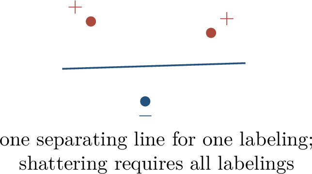
One must also be careful not to confuse VC dimension with parameter count. The class \[\mathcal{H} = \{x\mapsto \operatorname{sgn}(\sin(ax)):a\in\R\}\] has only one real parameter, yet it has infinite VC dimension on the real line: by taking \(a\) large enough, the sine wave can oscillate rapidly enough to match arbitrary alternating patterns on carefully chosen points.
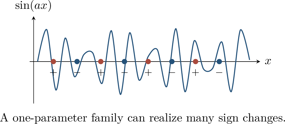
Definition 0.15 (Growth function). For \(T=\{x_1,\ldots,x_N\}\subset\mathcal{X}\), define the set of label patterns realized by \(\mathcal{H}\) on \(T\) by \[\mathcal{H}(T) = \{(h(x_1),\ldots,h(x_N)):h\in\mathcal{H}\}.\] The growth function is \[G_\mathcal{H}(N) = \max_{x_1,\ldots,x_N\in\mathcal{X}} \left\lvert \mathcal{H}(\{x_1,\ldots,x_N\}) \right\rvert.\] Thus \(T\) is shattered if and only if \(\left\lvert \mathcal{H}(T) \right\rvert=2^{|T|}\).
Lemma 0.8 (Sauer–Shelah lemma). If \(\operatorname{VCdim}(\mathcal{H})=k\), then for every \(N\), \[G_\mathcal{H}(N) \le \sum_{i=0}^k \binom{N}{i}.\] In particular, when \(N>k\), \[G_\mathcal{H}(N) \le \left(\frac{eN}{k}\right)^k .\]
The significance of the Sauer–Shelah lemma is that finite VC dimension turns an infinite class into a polynomial-size collection of label patterns on any finite sample. This is the bridge from finite-class counting to infinite classes.
Before the VC dimension is reached, the growth function may be as large as \(2^N\). After the VC dimension is exceeded, the Sauer–Shelah lemma forces a sharp change from exponential growth to polynomial growth. This is why finite VC dimension is a capacity notion: it does not say the class is finite, but it says the class cannot keep encoding independent bits on arbitrarily large samples.
Theorem 0.8 (VC uniform convergence). Let \(\mathcal{H}\) be a class of binary classifiers with \(\operatorname{VCdim}(\mathcal{H})=k\). There is a universal constant \(C>0\) such that if \[N \ge \frac{C}{\epsilon^2} \left( k\log\frac{1}{\epsilon}+\log\frac{1}{\delta} \right),\] then, with probability at least \(1-\delta\), \[\forall h\in\mathcal{H},\qquad \left\lvert \operatorname{err}_\mathcal{D}(h)-\operatorname{err}_S(h) \right\rvert \le \epsilon .\] Equivalently, a common high-probability form is \[\operatorname{err}_\mathcal{D}(h) \le \operatorname{err}_S(h) + \sqrt{ \frac{ C\{k\log(N/k)+\log(1/\delta)\} }{N} } \qquad \text{for all }h\in\mathcal{H}.\]
3.0.3.1 Proof idea: ghost samples and Rademacher signs
The proof follows the same logic as the finite-class proof, but the counting is performed after restricting the hypotheses to a random finite set. Let \(S'=\{(x_i',y_i')\}_{i=1}^N\) be an independent ghost sample. One first controls the expected uniform gap by replacing the unknown population error by the empirical error on \(S'\): \[\E_S\sup_{h\in\mathcal{H}} \left\lvert \operatorname{err}_\mathcal{D}(h)-\operatorname{err}_S(h) \right\rvert \le \E_{S,S'}\sup_{h\in\mathcal{H}} \left\lvert \operatorname{err}_{S'}(h)-\operatorname{err}_S(h) \right\rvert .\] The reference notes emphasize the role of Jensen’s inequality here: the supremum is convex, so the expectation over the ghost sample can be brought inside an upper bound.
Now condition on the \(2N\) examples in \(S\cup S'\). For each pair \((z_i,z_i')=((x_i,y_i),(x_i',y_i'))\), flip an independent Rademacher sign \(\sigma_i\in\{-1,+1\}\) to decide which point is viewed as belonging to \(S\) and which to \(S'\). This symmetrization gives expressions of the form \[\E_{S,S',\sigma} \sup_{h\in\mathcal{H}} \left\lvert \frac{1}{N} \sum_{i=1}^N \sigma_i \left( \mathbf{1}{h(x_i)\ne y_i} - \mathbf{1}{h(x_i')\ne y_i'} \right) \right\rvert .\] Once the \(2N\) examples are fixed, hypotheses that agree on these examples are interchangeable. Therefore one needs to union bound only over the patterns in \(\mathcal{H}(S\cup S')\), whose cardinality is at most \[G_\mathcal{H}(2N) \le \left(\frac{2eN}{k}\right)^k .\] For each fixed pattern, the Rademacher sum is sub-Gaussian: \[\Prob\left[ \left\lvert \frac{1}{N}\sum_{i=1}^N \sigma_i(a_i-a_i') \right\rvert > \epsilon \right] \le 2e^{-N\epsilon^2/2}.\] Combining this tail bound with the growth-function count produces the VC rate.
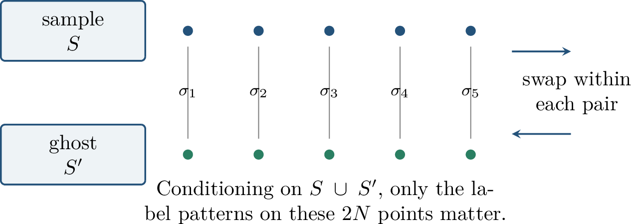
3.0.4 VC Bounds for Neural Networks↩︎
We now return to neural networks. To keep the combinatorics transparent, the chapter considers sign-activation networks. Let the architecture have layer widths \(d_0,d_1,\ldots,d_L\), and define \[f=f_L\circ f_{L-1}\circ\cdots\circ f_1, \qquad f_i(x)=\operatorname{sgn}(A_i x+b_i),\] where \(A_i\in\R^{d_i\times d_{i-1}}\) and \(b_i\in\R^{d_i}\). The number of scalar parameters is \[p=\sum_{i=1}^L d_i(d_{i-1}+1).\]
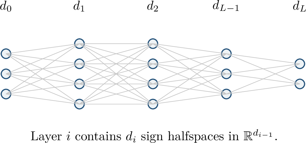
Theorem 0.9 (VC dimension of sign networks). For a fixed architecture with \(p\) scalar parameters, the class of sign networks described above satisfies \[\operatorname{VCdim}(\mathcal{H})=O(p\log p).\]
The proof in the chapter is a growth-function proof. It uses two elementary rules.
Lemma 0.9 (Product rule for growth functions). Let \(\mathcal{H}_1\subseteq \mathcal{Y}_1^\mathcal{X}\) and \(\mathcal{H}_2\subseteq \mathcal{Y}_2^\mathcal{X}\). For the product class \(\mathcal{H}=\mathcal{H}_1\times\mathcal{H}_2\), meaning \[x\mapsto (h_1(x),h_2(x)), \qquad h_1\in\mathcal{H}_1,\;h_2\in\mathcal{H}_2,\] we have \[G_\mathcal{H}(N)\le G_{\mathcal{H}_1}(N)G_{\mathcal{H}_2}(N).\]
Proof. Fix any \(N\)-point set \(T\subset\mathcal{X}\). The first coordinate of a pattern realized by \(\mathcal{H}\) on \(T\) must be a pattern realized by \(\mathcal{H}_1\) on \(T\), and the second coordinate must be a pattern realized by \(\mathcal{H}_2\) on \(T\). Thus \[\left\lvert \mathcal{H}(T) \right\rvert \le \left\lvert \mathcal{H}_1(T) \right\rvert\,\left\lvert \mathcal{H}_2(T) \right\rvert \le G_{\mathcal{H}_1}(N)G_{\mathcal{H}_2}(N).\] Taking the maximum over \(T\) proves the claim. ◻
Lemma 0.10 (Composition rule for growth functions). Let \(\mathcal{H}_1\subseteq \mathcal{Y}_1^\mathcal{X}\) and \(\mathcal{H}_2\subseteq \mathcal{Y}_2^{\mathcal{Y}_1}\). For the composition class \(\mathcal{H}=\mathcal{H}_2\circ\mathcal{H}_1\), we have \[G_\mathcal{H}(N)\le G_{\mathcal{H}_1}(N)G_{\mathcal{H}_2}(N).\]
Proof. Fix \(T=\{x_1,\ldots,x_N\}\). First choose the intermediate pattern \[(h_1(x_1),\ldots,h_1(x_N))\] produced by some \(h_1\in\mathcal{H}_1\). There are at most \(G_{\mathcal{H}_1}(N)\) such patterns. Once this intermediate pattern is fixed, the functions in \(\mathcal{H}_2\) can produce at most \(G_{\mathcal{H}_2}(N)\) output patterns on these \(N\) intermediate points. Multiplying these two counts and maximizing over \(T\) gives the desired inequality. ◻
Proof idea of the sign-network bound. For the \(j\)-th neuron in layer \(i\), the relevant hypothesis class is a set of halfspaces in \(\R^{d_{i-1}}\). Its VC dimension is \(d_{i-1}+1\), so the Sauer–Shelah lemma gives \[G_{\mathcal{H}_{(i,j)}}(N) \le \left(\frac{eN}{d_{i-1}+1}\right)^{d_{i-1}+1} \le (eN)^{d_{i-1}+1}.\] The product rule combines the neurons in a layer, and the composition rule combines the layers: \[G_\mathcal{H}(N) \le \prod_{i=1}^L \prod_{j=1}^{d_i} G_{\mathcal{H}_{(i,j)}}(N) \le (eN)^p.\] If \(\mathcal{H}\) shatters a set \(S\) of size \(N\), then \[2^N=\left\lvert \mathcal{H}(S) \right\rvert\le (eN)^p.\] Solving this inequality gives \(N=O(p\log p)\). Hence the largest shattered set has size \(O(p\log p)\). ◻
The logarithmic factor appears when one solves \(2^N\le(eN)^p\). Taking logarithms gives \(N\log 2\le p(1+\log N)\), so a shattered set cannot be much larger than a constant multiple of \(p\log p\). The argument is intentionally coarse: it counts all possible sign patterns that could be produced by the architecture, without asking which patterns are likely on natural data or which patterns gradient-based training will actually reach.
This is a beautiful result, but it also explains why worst-case VC bounds are often vacuous for modern networks. The useful VC bound becomes nontrivial only when \(N\) is at least on the order of the number of parameters. Many deep networks used in practice have \(p\gg N\) and can fit arbitrary labels, yet they still generalize on natural data. Worst-case counting is therefore insufficient; it does not see the structure of the data distribution, the optimization path, or the particular solution chosen by training.
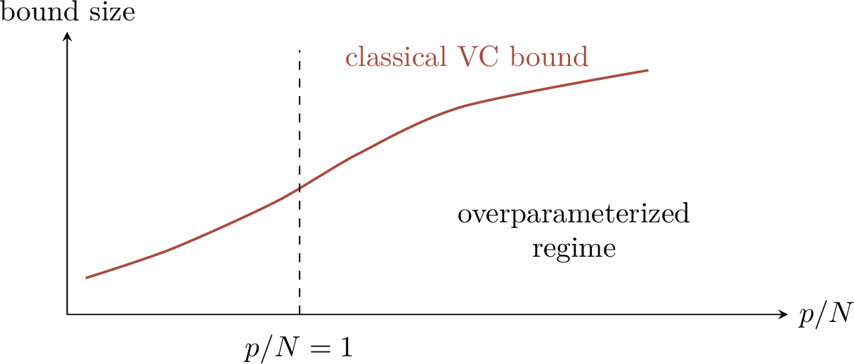
3.0.5 PAC Learnability↩︎
VC dimension is not merely a proof technique for a convenient bound. In the distribution-free realizable setting, it exactly characterizes learnability.
Definition 0.16 (PAC learnability). A binary concept class \(\mathcal{H}\) is PAC learnable if for every distribution \(\mathcal{D}\) on \(\mathcal{X}\), every target \(h^\star\in\mathcal{H}\), and every \(\epsilon,\delta>0\), there is an algorithm that uses \(N(\epsilon,\delta,\mathcal{H})\) examples \((x_i,h^\star(x_i))\) with \(x_i\sim\mathcal{D}\) and returns \(h\in\mathcal{H}\) satisfying \[\Prob_{x\sim\mathcal{D}}\!\left[h(x)\ne h^\star(x)\right]\le \epsilon\] with probability at least \(1-\delta\) over the training sample.
Theorem 0.10 (Blumer–Ehrenfeucht–Haussler–Warmuth). A binary concept class \(\mathcal{H}\) is PAC learnable if and only if \(\operatorname{VCdim}(\mathcal{H})<\infty\).
This theorem is one of the central structural results of classical learning theory. It says that finite VC dimension is not merely sufficient for a particular proof technique; it is exactly the right distribution-free combinatorial condition for binary concept learning. The result is independent of the parameterization used to describe \(\mathcal{H}\). What matters is the set of labelings the class can impose on finite samples.
The finite-VC direction follows from uniform convergence. In the realizable case, empirical risk minimization returns a zero-training-error classifier, and one obtains sample complexity of order \[N = O\left( \frac{k\log(1/\epsilon)+\log(1/\delta)}{\epsilon} \right), \qquad k=\operatorname{VCdim}(\mathcal{H}).\] The infinite-VC direction is a no-free-lunch argument. If \(\mathcal{H}\) shatters arbitrarily large finite sets, then for a large shattered set \(T\) and the uniform distribution on \(T\), the target labels can be arbitrary bits. Until the learner has observed most of the points, the labels on unseen points remain compatible with many possible targets. No distribution-free algorithm can guess them reliably.
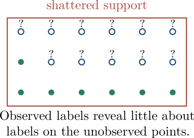
The same characterization extends to the noisy, agnostic setting: a concept class is agnostically PAC learnable if and only if it has finite VC dimension. In that setting the goal is to return \(h\) with \(\operatorname{err}_\mathcal{D}(h)\le \inf_{g\in\mathcal{H}}\operatorname{err}_\mathcal{D}(g)+\epsilon\), rather than to recover a realizable target exactly.
3.0.6 Sample-Dependent Bounds↩︎
VC theory is distribution-free and worst-case. That strength is also its weakness for deep learning: it treats the sample as if it could be the most adversarial finite set for the architecture. A more refined question is whether the class can correlate with random labels on typical samples from the data distribution.
Definition 0.17 (Empirical random-label complexity). For a binary classifier class \(\mathcal{H}\), define \[\mathfrak{R}_N(\mathcal{H}) = \E_S\E_\sigma \left[ \sup_{h\in\mathcal{H}} \left\lvert \frac{1}{N}\sum_{i=1}^N \sigma_i\mathbf{1}{h(x_i)\ne y_i} \right\rvert \right],\] where \(\sigma_1,\ldots,\sigma_N\) are independent random signs taking values \(\pm1\).
Intuitively, \(\mathfrak{R}_N(\mathcal{H})\) measures how well \(\mathcal{H}\) can align with random noise on samples drawn from the distribution. If the best classifier in \(\mathcal{H}\) has only weak correlation with random signs, then the class has limited effective capacity on typical data, even if its worst-case VC dimension is large.
Theorem 0.11 (Data-dependent uniform convergence). With probability at least \(1-\delta\), \[\sup_{h\in\mathcal{H}} \left\lvert \operatorname{err}_\mathcal{D}(h)-\operatorname{err}_S(h) \right\rvert \le 2\,\mathfrak{R}_N(\mathcal{H}) + \sqrt{\frac{\log(2/\delta)}{2N}}.\]
The proof is another symmetrization argument. The first term compares the sample to an independent ghost sample, and the random signs measure how much the class can change when the two samples are swapped. The final square-root term is the concentration cost for moving from the expected complexity to a high-probability statement. Unlike the VC bound, this quantity is distribution-dependent because the expectation is taken over samples drawn from \(\mathcal{D}\).
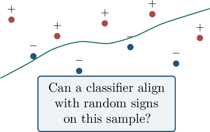
3.0.6.1 Random labels and deep networks
A tempting hope is that although a deep network has large VC dimension, the combination of natural data and SGD might prevent it from fitting random labels. The random-label experiments of Zhang et al. showed that this hope is false in a strong sense: sufficiently expressive deep networks trained by SGD can fit randomly assigned labels almost perfectly on real inputs. The result does not say that deep networks cannot generalize; rather, it says that architecture-only bounds and naive Rademacher explanations are usually too weak. To obtain informative statements, one must also use margins, norms, compression, priors, data geometry, or algorithmic bias [35].
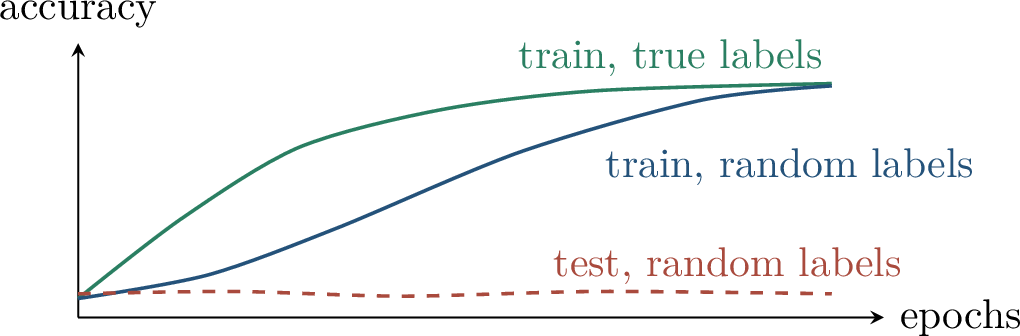
3.0.7 Margins, Fat Shattering, and PAC-Bayes↩︎
The last part of the chapter surveys two ways to describe a learned hypothesis more finely than by raw parameter count. Margin bounds use real-valued function values and norms. PAC-Bayes bounds describe how much a data-dependent posterior over predictors deviates from a data-independent prior.
Definition 0.18 (Fat-shattering dimension). Let \(\mathcal{H}\) be a real-valued function class on \(\mathcal{X}\). Points \(x_1,\ldots,x_N\) are \(\gamma\)-shattered by \(\mathcal{H}\) if there exist thresholds \(r_1,\ldots,r_N\in\R\) such that for every \((b_1,\ldots,b_N)\in\{-1,+1\}^N\) there exists \(h\in\mathcal{H}\) satisfying \[b_i\bigl(h(x_i)-r_i\bigr)\ge \gamma \qquad \text{for all } i=1,\ldots,N .\] The fat-shattering dimension at scale \(\gamma\), denoted \(\operatorname{fat}_\mathcal{H}(\gamma)\), is the largest \(N\) for which such points exist.
The scale \(\gamma\) is crucial. A real-valued class may separate many points with tiny margins but far fewer points with a robust margin. This connects generalization to norm control and to the margins achieved by the trained network.
Fat shattering should be viewed as the real-valued analogue of VC dimension. If \(\gamma=0\) and the thresholds are all zero, the condition resembles ordinary shattering by signs. For positive \(\gamma\), however, each label must be realized with a buffer. This buffer makes the statement stable: small perturbations of the function values do not immediately change the induced classification.
Theorem 0.12 (A Bartlett-style margin bound). Consider depth-\(L\) networks on \[\mathcal{X}=\{x\in\R^n:\left\lVert x \right\rVert_\infty\le B\},\] and suppose each hidden unit has incoming weight vector \(w\) satisfying \(\left\lVert w \right\rVert_1\le A\). For a universal constant \(c\), \[\operatorname{fat}_\mathcal{H}(\gamma) = O\left( \frac{ B^2(cA)^{L(L+1)} }{\gamma^{2L}} \log n \right).\]
The precise constants are less important here than the message: margin and norm constraints can yield an effective capacity much smaller than what raw parameter counting suggests. Later refinements replace the simple \(\ell_1\)-weight control above by sharper spectral, path-norm, compression, or margin-sensitive quantities. The theorem is representative of the classical line of margin-based neural-network bounds in which the size of the weights, rather than the mere number of parameters, controls sample complexity [13].
Definition 0.19 (PAC-Bayes setup). Let \(P\) be a data-independent prior distribution over hypotheses, and let \(Q\) be a posterior distribution that may be chosen after seeing the sample \(S\). Define the Gibbs population and empirical errors by \[\operatorname{err}_\mathcal{D}(Q)=\E_{h\sim Q}\operatorname{err}_\mathcal{D}(h), \qquad \operatorname{err}_S(Q)=\E_{h\sim Q}\operatorname{err}_S(h).\]
Theorem 0.13 (McAllester-style PAC-Bayes bound). For \(0<\gamma<1\) and \(\delta>0\), with probability at least \(1-\delta\) over the sample, every posterior \(Q\) satisfies \[\operatorname{err}_\mathcal{D}(Q) \le \frac{1}{\gamma}\operatorname{err}_S(Q) + \frac{ \KL(Q\|P)+\log(1/\delta) }{ 2\gamma(1-\gamma)N } .\]
The term \(\KL(Q\|P)\) is a description length: it measures how much the posterior learned from the data differs from the reference distribution chosen before seeing the data. If \(Q\) fits the sample and remains close to \(P\), the bound can be nonvacuous even for overparameterized networks. This viewpoint led to influential nonvacuous PAC-Bayes certificates for MNIST-scale networks.
The prior must be chosen independently of the sample. Otherwise the KL term would no longer represent information extracted from the data, and the bound would lose its statistical meaning. The posterior, by contrast, is allowed to depend on the sample. PAC-Bayes theory therefore formalizes a tradeoff: learning may adapt to the data, but it pays for the amount of adaptation through \(\KL(Q\|P)\).
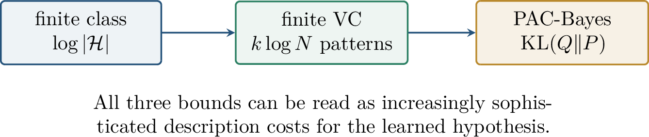
3.0.8 What the Bounds Explain, and What They Do Not↩︎
Classical generalization theory explains several fundamental facts. It shows why finite or low-VC classes are learnable, why sample size must grow with capacity, and why distribution-free learning is impossible for classes with infinite VC dimension. It also gives a vocabulary for more refined description-based bounds: margins, norms, compression, and KL divergence.
At the same time, the chapter is careful about what these results do not explain by themselves. Worst-case uniform convergence does not explain why large overparameterized networks generalize on natural data. It does not explain why optimization selects some interpolating solutions rather than others, or why margins, norms, compression, and flatness often track test error better than parameter count. It also does not address distribution shift, adversarial robustness, or transfer learning.
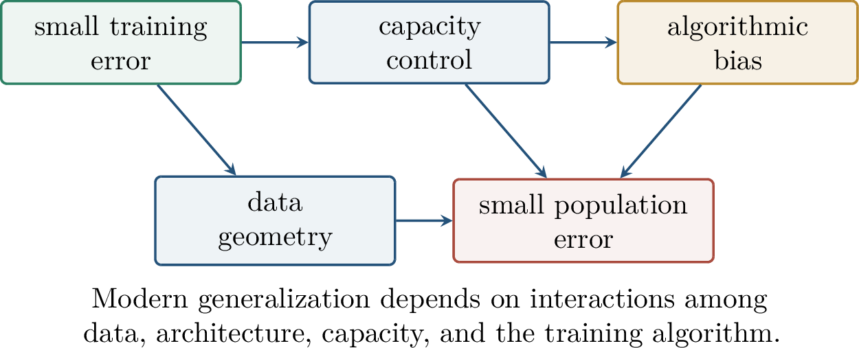
The conceptual endpoint of the chapter is therefore not that VC theory is wrong. On the contrary, finite VC dimension is a tight characterization of distribution-free PAC learnability. The point is that the guarantees one gets from worst-case counting are often too coarse for deep learning practice. This motivates the more refined theories that appear throughout the rest of the framework: norm and margin control, compression, PAC-Bayes analysis, implicit regularization, stability, and distribution-sensitive descriptions of learned representations.
Chapter Synthesis This chapter developed generalization bounds as ways to control the gap between empirical and population error. For finite classes, Hoeffding’s inequality and a union bound give a \(\sqrt{\log|\mathcal{H}|/N}\) uniform-convergence rate, while the realizable case yields a sharper one-sided Occam bound. VC theory replaces the size of an infinite class by its growth function and VC dimension, leading to the distribution-free PAC characterization. For neural networks, worst-case VC bounds scale at least like parameter counts and are often vacuous in the overparameterized regime. This motivates sample-dependent, margin-based, and PAC-Bayes bounds, which try to measure the particular predictor, data distribution, and training outcome rather than only the raw architecture.
The chapter is based on the Chapter 5 Beamer source 408lec5_generalization_bounds and the reference note 408lec5post.pdf. Useful background sources include Vapnik’s statistical learning theory text [1], the learning theory textbook of Shalev-Shwartz and Ben-David [2], Bartlett’s margin and weight-size bounds for neural networks [13], and the random-label experiments of Zhang et al. [35]. PAC-Bayes analyses provide a
parallel description-length viewpoint that complements the VC and margin perspectives emphasized in this chapter.
3.0.9 Why Stability?↩︎
The previous chapter treated generalization mostly through the size or complexity of a hypothesis class. Stability gives a different language. It asks not how large the class is, but how much the algorithmic output changes when one training example is replaced. If a single observation can dramatically alter the learned predictor, then the empirical loss has become too tied to the sample. If replacing one observation changes predictions or losses only slightly, then the training sample is acting like a reliable proxy for new data.
This is a shift from class-based to algorithm-based reasoning. A VC or uniform-convergence bound controls all hypotheses in a class at once. A stability bound controls the output of the particular algorithm being run. This distinction matters in deep learning because the ambient class may be large enough to fit arbitrary labels, while the training procedure may still select predictors that are insensitive to individual examples. Stability therefore connects naturally to regularization, early stopping, stochastic optimization, and privacy [14].
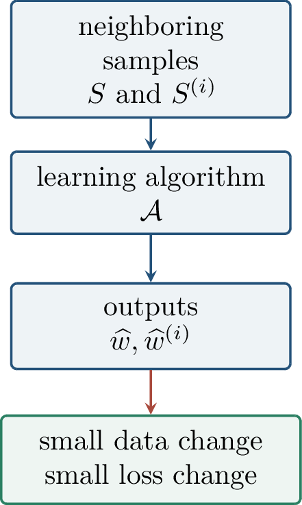
Definition 0.20 (Risk, empirical risk, and generalization error). Let \(z=(x,y)\sim\mathcal{D}\), and let \[S=(z_1,\ldots,z_N)\sim\mathcal{D}^N\] be an iid training sample. For a parameter \(w\in\Omega\), define \[R(w)=\E_{z\sim\mathcal{D}}\ell(w,z), \qquad R_S(w)=\frac{1}{N}\sum_{i=1}^N \ell(w,z_i).\] The generalization error of \(w\) on \(S\) is \[\epsilon_{\mathrm{gen}}(w)=R(w)-R_S(w).\] For a learning algorithm, the output \(\mathcal{A}(S)\) is random because it depends on the random sample, and possibly also on internal algorithmic randomness.
The sign convention in \(\epsilon_{\mathrm{gen}}(w)=R(w)-R_S(w)\) is intentional. A positive generalization gap means that the empirical risk underestimates the population risk at the learned parameter. For a fixed \(w\), this gap has mean zero. For \(w=\mathcal{A}(S)\), the same is no longer true because the parameter has been chosen using the sample whose empirical risk is being measured.
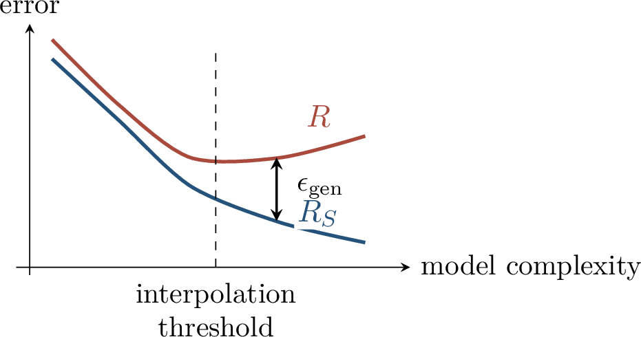
3.0.9.1 Explicit and implicit regularization
Stability often comes from regularization. Sometimes the regularizer is explicit, as in \[\min_w\; R_S(w)+\frac{\alpha}{2}\left\lVert w \right\rVert_2^2 .\] The quadratic penalty adds curvature and discourages sensitivity. Sometimes the regularizer is implicit: stochastic gradient descent, \[w_{t+1}=w_t-\eta_t\nabla\ell(w_t,z_{i_t}),\] has step sizes, stopping times, initialization, and sampling noise that bias the selected solution. The two mechanisms are not identical, but both can make the learned predictor less dependent on any single training point.
Regularization should be understood here in the broad algorithmic sense. A penalty term changes the objective directly. Step sizes, initialization, and stopping time change the path through parameter space. Both mechanisms may reduce sensitivity, but they do so through different mathematical objects: the former usually through curvature of an objective, the latter through a coupling argument for the dynamics.
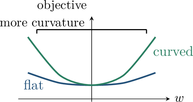
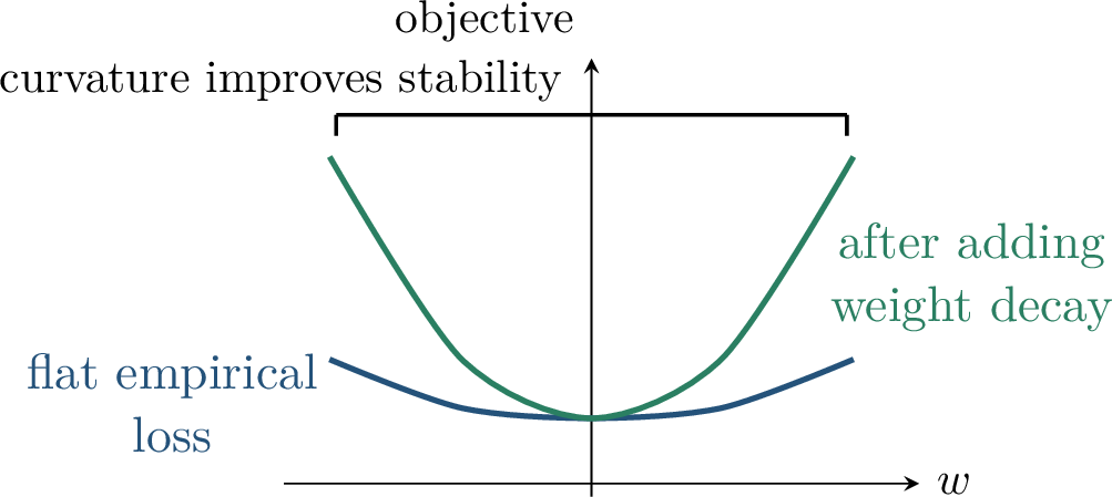
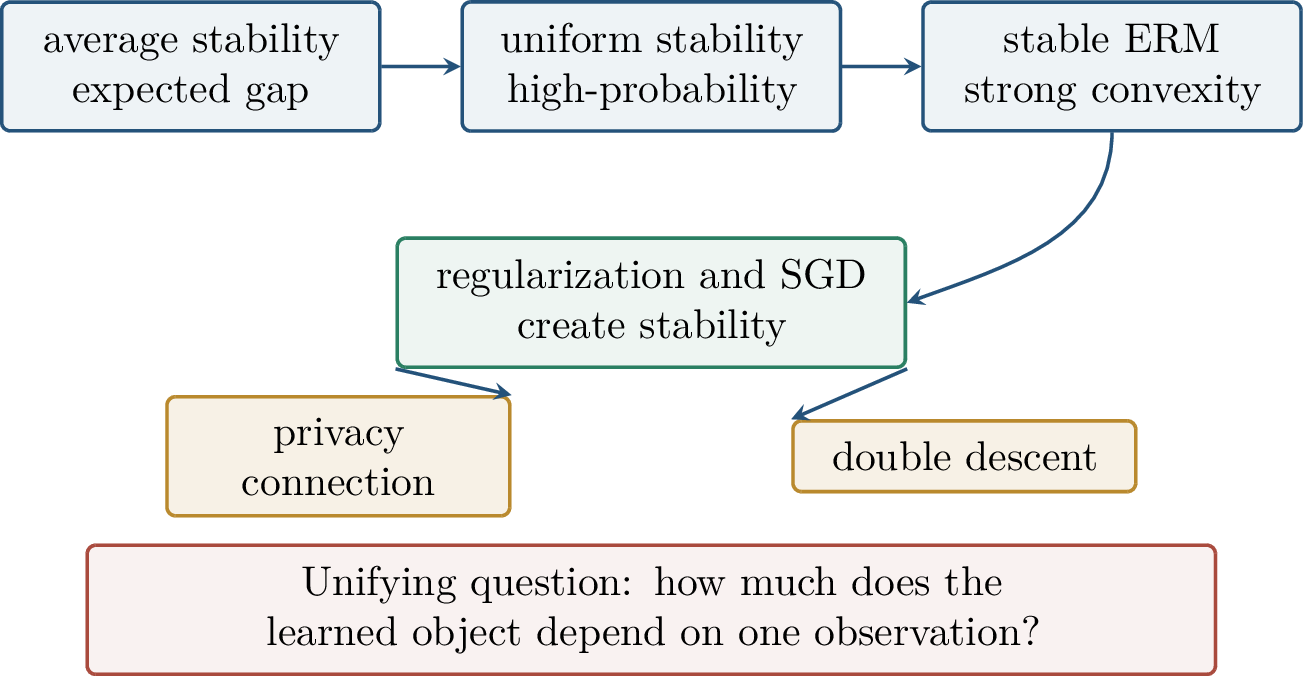
3.0.10 Average Stability↩︎
The stability viewpoint treats a learning algorithm as a map \[\mathcal{A}:\mathcal{Z}^N\to\Omega,\qquad S\mapsto \mathcal{A}(S).\] For randomized algorithms, the map also depends on internal randomness, and expectations below include that randomness when appropriate.
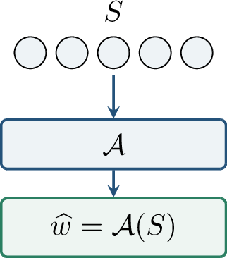
Let \(S=(z_1,\ldots,z_N)\) and \(S'=(z_1',\ldots,z_N')\) be independent iid samples. The hybrid sample that replaces only the \(i\)-th point is \[S^{(i)} = (z_1,\ldots,z_{i-1},z_i',z_{i+1},\ldots,z_N).\] The point \(z_i'\) will play a double role: it is both the replacement point and the test point at which the loss change is measured.
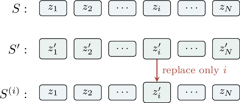
Definition 0.21 (Average stability). The average stability of \(\mathcal{A}\) is \[\begin{align} \Delta(\mathcal{A}) &= \E_{S,S'} \left[ \frac{1}{N}\sum_{i=1}^N \left( \ell(\mathcal{A}(S),z_i') - \ell(\mathcal{A}(S^{(i)}),z_i') \right) \right]. \end{align}\]
This quantity is an average over samples and replacement positions. It can be negative for some algorithms because it is a signed difference, but its connection to expected generalization is exact.
The definition may look asymmetric because the loss is evaluated at \(z_i'\), the point inserted into the hybrid sample. This choice is what makes the identity below work cleanly. The ghost sample represents fresh data from \(\mathcal{D}\), while the hybrid sample lets us compare the algorithm trained with and without the particular point whose loss is being tested.
Theorem 0.14 (Average stability identity). For any learning algorithm \(\mathcal{A}\) and iid training set \(S\), \[\E_S\!\left[\epsilon_{\mathrm{gen}}(\mathcal{A}(S))\right]=\Delta(\mathcal{A}).\]
Proof. Introduce an independent ghost sample \(S'\). Since \(z_i'\sim\mathcal{D}\), \[\E_SR(\mathcal{A}(S)) = \E_{S,S'}\frac{1}{N}\sum_{i=1}^N \ell(\mathcal{A}(S),z_i').\] For the empirical term, use exchangeability of \(z_i\) and \(z_i'\). The sample \(S\) has the same distribution as \(S^{(i)}\) after swapping the two coordinates \(z_i\) and \(z_i'\), so \[\E_SR_S(\mathcal{A}(S)) = \E_{S,S'}\frac{1}{N}\sum_{i=1}^N \ell(\mathcal{A}(S^{(i)}),z_i').\] Subtracting the two identities gives the result. ◻
No concentration inequality is used in this argument. The identity is purely an exchangeability calculation: an iid sample does not remember which point was called the training point and which was called the ghost point. This is why average stability is a natural exact counterpart to expected generalization. The price is that average stability alone does not immediately provide a high-probability statement for a particular realized sample.
Average stability explains what the expected test–train gap is: it is the average loss change caused by replacing one example. The practical challenge is bounding \(\Delta(\mathcal{A})\). For high-probability guarantees, we usually impose a stronger worst-case stability condition.
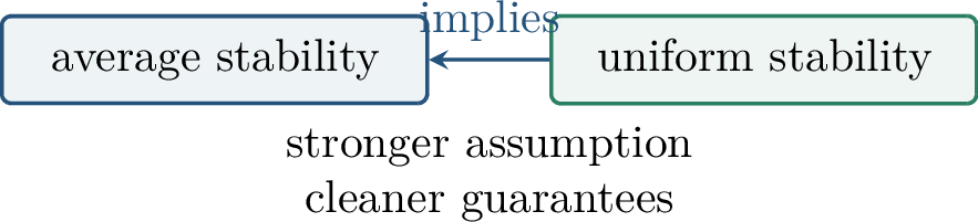
3.0.11 Uniform Stability↩︎
Definition 0.22 (Uniform stability). An algorithm \(\mathcal{A}\) is \(\gamma\)-uniformly stable if, for all neighboring samples \(S,S^{(i)}\) and all test points \(z\), \[\left\lvert \ell(\mathcal{A}(S),z)-\ell(\mathcal{A}(S^{(i)}),z) \right\rvert \le \gamma .\] We write \(\Delta_{\mathrm{unif}}(\mathcal{A})\le\gamma\).
This is a worst-case condition over the sample, the replaced coordinate, and the test point. The handwritten notes use the equivalent chapter version that tests at the replacement point \(z_i'\). The displayed definition is the standard stronger form and is the one most often used in generalization theorems.
Uniform stability is deliberately stringent. It requires the same loss-change bound for every neighboring pair of datasets and every possible test point. This worst-case nature is what makes it easy to convert into generalization guarantees, but it can also make the condition too strong for large nonconvex models. Much of the modern theory studies weaker or data-dependent stability notions that retain some of the same intuition.
Corollary 0.1 (Expected generalization from uniform stability). If \(\Delta_{\mathrm{unif}}(\mathcal{A})\le\gamma\), then \[\left\lvert \E_S\epsilon_{\mathrm{gen}}(\mathcal{A}(S)) \right\rvert\le\gamma.\]
Proof. Every summand in the average-stability identity is bounded in absolute value by \(\gamma\). Averaging and taking expectations cannot increase this bound. ◻
Theorem 0.15 (Feldman–Vondrak high-probability bound). Assume the loss is bounded and \(\mathcal{A}\) is \(\gamma\)-uniformly stable. With probability at least \(1-\delta\), \[\epsilon_{\mathrm{gen}}(\mathcal{A}(S)) \lesssim \gamma\,\log N\,\log\!\left(\frac{N}{\delta}\right) + \sqrt{\frac{\log(1/\delta)}{N}} .\]
The second term is the ordinary sampling fluctuation. The first term converts algorithmic sensitivity into a tail bound. The result is useful when \(\gamma\) is of order \(1/N\), up to logarithmic factors. It also clarifies a distinction from uniform convergence: we do not need to control every \(w\in\Omega\), only the particular output selected by the algorithm.
The logarithmic factors in the Feldman–Vondrak bound are not the main message for this monograph. The conceptual message is that a single-output sensitivity condition can replace a whole-class capacity condition. When \(\gamma\) is small, the algorithm cannot exploit idiosyncratic information in one training example very much, so its training loss is less likely to be overly optimistic.
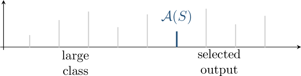
Most stability proofs follow a simple template. First prove that neighboring outputs are close: \[\left\lVert \mathcal{A}(S)-\mathcal{A}(S^{(i)}) \right\rVert\le\rho .\] Then use Lipschitzness of the loss, \[\left\lvert \ell(w,z)-\ell(w',z) \right\rvert \le L\left\lVert w-w' \right\rVert,\] to conclude \(\gamma\le L\rho\). Strong convexity is one of the cleanest ways to get the distance bound \(\rho\).
3.0.12 Stable Empirical Risk Minimization↩︎
Let empirical risk minimization return \[\widehat w_S\in \argmin_{w\in\Omega} \frac{1}{N}\sum_{i=1}^N\ell(w,z_i).\] We assume throughout this section that the minimizer is selected in a well-defined way whenever there are ties.
The core difficulty is that empirical risk minimizers can be unstable when the objective is flat near its minimum. A small change in one summand may then move the selected minimizer a long distance along a nearly flat valley. Strong convexity rules this out by forcing the objective to grow quadratically away from its minimizer. This is the same geometric idea that appeared in explicit regularization: curvature turns small perturbations of an objective into small perturbations of its optimizer.
Definition 0.23 (Strong convexity and Lipschitzness). For a fixed \(z\), the loss \(\ell(\cdot,z)\) is \(\alpha\)-strongly convex if \[\ell(w',z) \ge \ell(w,z)+\nabla\ell(w,z)^\top(w'-w) +\frac{\alpha}{2}\left\lVert w'-w \right\rVert_2^2 .\] It is \(L\)-Lipschitz if \[\left\lvert \ell(w',z)-\ell(w,z) \right\rvert \le L\left\lVert w'-w \right\rVert_2 .\]
Strong convexity is a lower-curvature condition; Lipschitzness is an upper control on loss variation. The stability proof needs both. Curvature first shows that neighboring minimizers are close in parameter space, and Lipschitzness then translates this parameter-space closeness into a small change in loss at any test point.
Theorem 0.16 (Stability of strongly convex ERM). Suppose \(\ell(\cdot,z)\) is \(\alpha\)-strongly convex and \(L\)-Lipschitz for every \(z\). Then ERM is uniformly stable: \[\Delta_{\mathrm{unif}}(\mathrm{ERM})\le \frac{4L^2}{\alpha N}.\]
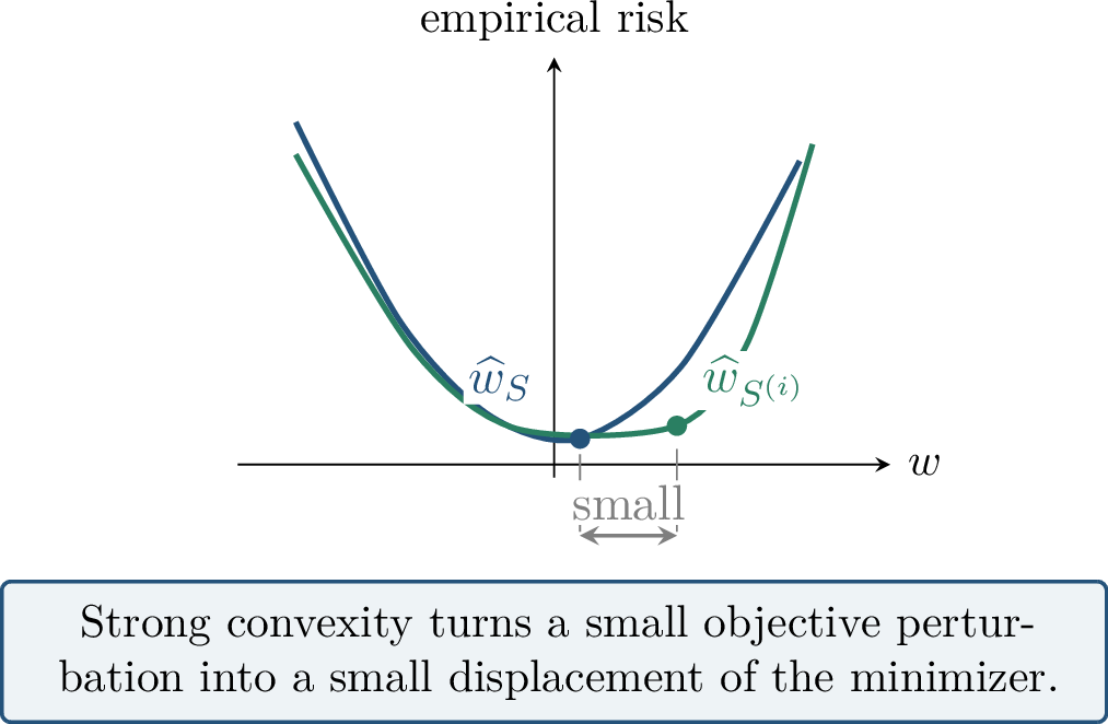
Lemma 0.11 (Convex combinations preserve curvature). If \(f\) and \(g\) are both \(\alpha\)-strongly convex, then for \(0\le\lambda\le1\), \[h=\lambda f+(1-\lambda)g\] is also \(\alpha\)-strongly convex.
Proof. Apply the strong-convexity inequality to \(f\) and \(g\), multiply the two inequalities by \(\lambda\) and \(1-\lambda\), and add them. The linear terms and the quadratic curvature terms combine with the same coefficient \(\alpha\). ◻
Proof sketch of the ERM stability theorem. By the lemma, the empirical risk \(R_S\) is \(\alpha\)-strongly convex. Since \(\widehat w_S\) minimizes \(R_S\), \[R_S(\widehat w_{S^{(i)}})-R_S(\widehat w_S) \ge \frac{\alpha}{2} \left\lVert \widehat w_{S^{(i)}}-\widehat w_S \right\rVert_2^2 .\] On the other hand, comparing the empirical objectives on \(S\) and \(S^{(i)}\) and using optimality of both minimizers, the fact that only one summand has changed, and \(L\)-Lipschitzness, gives \[R_S(\widehat w_{S^{(i)}})-R_S(\widehat w_S) \le \frac{2L}{N} \left\lVert \widehat w_{S^{(i)}}-\widehat w_S \right\rVert_2 .\] Combining the two displays yields \[\left\lVert \widehat w_{S^{(i)}}-\widehat w_S \right\rVert_2 \le \frac{4L}{\alpha N}.\] Finally, for every test point \(z\), \[\left\lvert \ell(\widehat w_{S^{(i)}},z)-\ell(\widehat w_S,z) \right\rvert \le L\left\lVert \widehat w_{S^{(i)}}-\widehat w_S \right\rVert_2 \le \frac{4L^2}{\alpha N}.\] ◻
The constants in this proof are less important than the scaling \(\gamma=O(1/(\alpha N))\). More samples make each individual summand less important; more curvature makes the minimizer harder to move. This scaling is the template behind many regularization-based stability results.

3.0.13 Regularization, SGD, and Privacy↩︎
3.0.13.1 Explicit regularization
When the original loss is convex but not strongly convex, one can add a quadratic penalty: \[F_S(w)=R_S(w)+\frac{\alpha}{2}\left\lVert w \right\rVert_2^2, \qquad \widehat w_S(\alpha)\in\argmin_{w\in\Omega}F_S(w).\] This makes the objective \(\alpha\)-strongly convex, but it introduces bias: the regularized population optimum may differ from the unregularized optimum.
The regularization parameter therefore has two jobs that pull in opposite directions. If \(\alpha\) is too small, the objective is nearly flat and the algorithm may be sensitive to individual samples. If \(\alpha\) is too large, the penalty dominates and the learned parameter is biased toward the origin. The theorem below makes this stability-bias tradeoff quantitative.
Theorem 0.17 (Regularized ERM bound). Assume \(\ell\) is convex and \(L\)-Lipschitz, and suppose \(\Omega\) has radius at most \(B\). For the choice \[\alpha = \sqrt{\frac{16L^2}{\delta B^2N}},\] with probability at least \(1-\delta\), \[R(\widehat w_S(\alpha))-R^\star \le 4\sqrt{\frac{L^2B^2}{\delta N}} \left(1+\frac{8}{\delta N}\right),\] where \(R^\star=\inf_{w\in\Omega}R(w)\).
The proof decomposes the excess risk into two terms. The stability term decreases when \(\alpha\) is large, because the objective is more curved. The bias term increases with \(\alpha\), because the penalty changes the population objective. Balancing these terms produces the displayed choice of \(\alpha\).
This bound is not meant to be the final word on regularization in deep networks. Its role in the chapter is pedagogical: it shows a complete calculation in which an explicit penalty creates stability, stability controls generalization, and the price of the penalty appears as approximation bias.
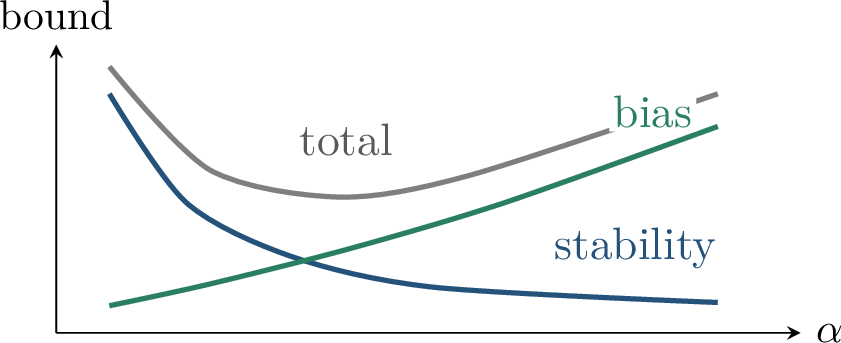
3.0.13.2 Implicit regularization by SGD
Stochastic gradient descent can also be stable without an explicit quadratic penalty. The reason is dynamic: two coupled runs on neighboring samples see the same example most of the time, and can drift only when the replaced example is selected.
This is an algorithmic version of regularization. Rather than modifying the objective, SGD limits how much information from any one example can propagate through the trajectory. If the step sizes are small, a hit to the replaced example causes only a small perturbation. If the number of steps is not too large, these perturbations do not have enough time to accumulate into a large loss difference. This viewpoint is central in the stability analysis of SGD [15].
Theorem 0.18 (Stability of SGD). Suppose each \(\ell(\cdot,z)\) is convex, \(\beta\)-smooth, and \(L\)-Lipschitz. Run SGD with step sizes \(\eta_t\le 2/\beta\) for \(T\) steps. Then \[\Delta_{\mathrm{unif}}(\mathrm{SGD}) \le \frac{2L^2}{N} \sum_{t=1}^T \eta_t .\]
Thus stability accumulates over time. Smaller step sizes and earlier stopping act as implicit regularizers. For example, with \(\eta_t\asymp N^{-1/2}\) and \(T=O(N)\), the bound scales like \(N^{-1/2}\).
The dependence on \(\sum_t\eta_t\) is worth reading literally. Long training with large step sizes can weaken the bound even if the empirical objective keeps decreasing. Early stopping is therefore not only an optimization heuristic; in stability theory it is a way to limit the cumulative influence of individual examples.
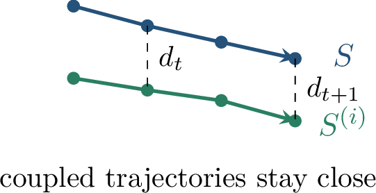
Definition 0.24 (Expected uniform stability). For a randomized algorithm, one common stability notion is \[\sup_{S,S^{(i)},z} \left\lvert \E_{\mathcal{A}}\!\left[ \ell(\mathcal{A}(S),z)-\ell(\mathcal{A}(S^{(i)}),z) \right] \right\rvert \le \gamma ,\] where the expectation is over the algorithm’s internal randomness.
The expectation is necessary because two SGD runs on neighboring samples are usually compared under a shared random seed or shared sequence of sampled indices. Stability is then a statement about the average loss difference under this coupling. This is weaker than deterministic uniform stability but often better matched to randomized training algorithms.
3.0.13.3 Connection to differential privacy
Differential privacy is another formal way to say that one data point should not strongly affect the algorithmic output. Stability controls losses on test points; privacy controls the entire output distribution.
The distinction between loss stability and output privacy is subtle but important. Two outputs may be far apart in parameter space while giving almost identical predictions, in which case stability can hold even when privacy fails. Conversely, a private algorithm may add enough noise to hide individual data points while still having a nontrivial prediction error. The two notions share a single-sample sensitivity philosophy, but they measure sensitivity in different spaces.
Definition 0.25 (Differential privacy). A randomized algorithm \(\mathcal{A}\) is \((\varepsilon,\delta)\)-differentially private if for all neighboring samples \(S,S^{(i)}\) and measurable sets \(U\subseteq\Omega\), \[\Prob[\mathcal{A}(S)\in U] \le e^\varepsilon\Prob[\mathcal{A}(S^{(i)})\in U]+\delta .\]
If \(\mathcal{A}\) is \((\varepsilon,\delta)\)-differentially private, then any test trying to distinguish \(S\) from \(S^{(i)}\) using the algorithm output satisfies \[P_{\mathrm{FA}}+e^\varepsilon P_{\mathrm{MD}}\ge 1-\delta, \qquad e^\varepsilon P_{\mathrm{FA}}+P_{\mathrm{MD}}\ge 1-\delta .\]
Here \(P_{\mathrm{FA}}\) is the false-alarm probability and \(P_{\mathrm{MD}}\) is the missed-detection probability. When \(\varepsilon\) and \(\delta\) are small, an observer cannot reliably determine whether a particular data point was in the training set. The reference notes stress the subtle difference: privacy says the learned parameters or output distribution do not depend much on any one data point; uniform stability says the loss at any test point does not change much when one data point is replaced. Nuisance directions in parameter space may affect privacy even when they do not affect loss.
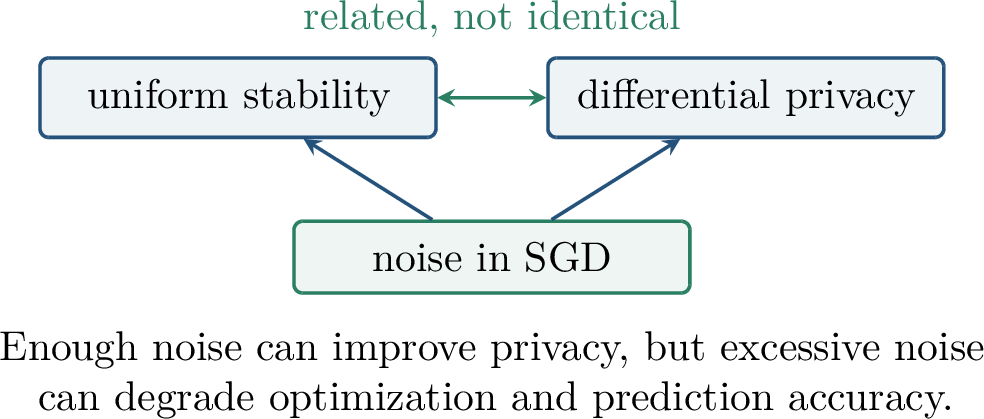
3.0.14 Double Descent↩︎
The classical bias–variance story says that as model capacity increases, bias decreases while variance increases, leading to a U-shaped test-error curve. Deep learning often operates beyond the interpolation threshold, where training error reaches zero. In this regime, test error can decrease again.
Double descent does not contradict the bias–variance decomposition. Instead, it shows that the behavior of the variance term near interpolation can be nonmonotone. At the interpolation threshold, the model has just enough degrees of freedom to fit the sample, so the fitted predictor can be extremely sensitive to noise. Far beyond the threshold, the optimizer may select a smoother or lower-norm interpolator, and the variance can decrease again. This phenomenon was emphasized in modern form by Belkin and collaborators [16].
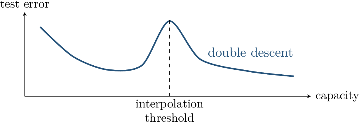
Let \[y=f(x)+\varepsilon, \qquad \E[\varepsilon\mid x]=0, \qquad \Var(\varepsilon\mid x)=\sigma^2,\] and let \(\widehat f(x;S)\) be the predictor learned from the random training set \(S\). Then \[\begin{align} \E_S\!\left[(y-\widehat f(x;S))^2\right] &= \underbrace{(\E_S\widehat f(x;S)-f(x))^2}_{\mathrm{bias}^2} \\ &\quad+ \underbrace{\E_S(\widehat f(x;S)-\E_S\widehat f(x;S))^2}_{\mathrm{variance}} +\sigma^2 . \end{align}\]
The three terms have different meanings. The irreducible noise \(\sigma^2\) is present even if the regression function \(f\) is known. The bias term measures systematic error caused by using an insufficient or constrained model class. The variance term measures sensitivity of the learned predictor to the random training sample. Double descent is largely about the variance term: interpolation can make variance explode near the threshold, but overparameterization plus a benign selection rule can make it decrease again.
Interpolation means zero training error. In linear regression it occurs when there are enough parameters to match the data. Once interpolation is possible, the essential question becomes: which interpolating solution does the optimizer choose?
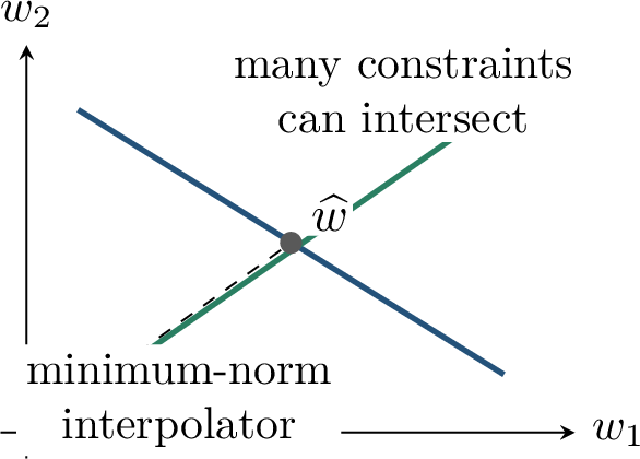
Definition 0.26 (Minimum-norm least-squares estimator). Consider \[y_i=x_i^\top\beta+\varepsilon_i, \qquad x_i\in\R^p,\quad i=1,\ldots,n,\] and let \(X\in\R^{n\times p}\), \(y\in\R^n\). The minimum-norm least-squares estimator is \[\widehat\beta = \argmin_b \left\{\left\lVert b \right\rVert_2: b\in\argmin_u\left\lVert y-Xu \right\rVert_2^2 \right\}.\] For \(p<n\), this is ordinary least squares when the solution is unique. For \(p>n\), it is the minimum-norm interpolating solution.
This estimator is also the limit of ridge regression as the ridge parameter tends to zero. In the overparameterized regime, the equations \(Xb=y\) have many solutions, and the minimum-norm rule selects the one orthogonal to the null space of \(X\). This is the linear analogue of the implicit-bias theme: zero training error is not enough to specify a predictor; an algorithmic or variational rule must select one interpolator.
Theorem 0.19 (High-dimensional ridgeless regression). Assume isotropic features, \(\Sigma=I\), and \(p/n\to\gamma\in(0,\infty)\). For the minimum-norm least-squares estimator, \[R(\widehat\beta,\beta) \to \begin{cases} \displaystyle \sigma^2\frac{\gamma}{1-\gamma}, & \gamma<1,\\[6pt] \displaystyle r^2\!\left(1-\frac{1}{\gamma}\right) +\frac{\sigma^2}{\gamma-1}, & \gamma>1, \end{cases}\] where \(r^2=\left\lVert \beta \right\rVert_2^2\). The risk diverges as \(\gamma\to1\).
The formula separates the underparameterized and overparameterized regimes. If \(\gamma<1\), ordinary least squares is unique and the variance term \(\sigma^2\gamma/(1-\gamma)\) grows as \(p\) approaches \(n\). If \(\gamma>1\), the estimator interpolates and the risk has two contributions: the term \(r^2(1-1/\gamma)\) reflects signal lost in directions that cannot be identified from the data, while \(\sigma^2/(\gamma-1)\) is the variance from fitting noise. The spike at \(\gamma=1\) is the interpolation peak. This ridgeless regression model is one of the cleanest solvable examples of double descent [36].
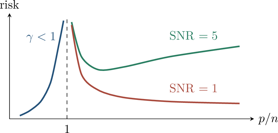
Let \(\mathrm{SNR}=r^2/\sigma^2\). The null predictor \(\widehat\beta=0\) has risk \(r^2\), and as \(\gamma\to\infty\) the ridgeless risk approaches this null risk. The reference notes emphasize two observations: regardless of SNR, the highly overparameterized limit converges to the null risk; and if the SNR is small, the overparameterized branch can be decreasing.
The null-risk limit should not be overinterpreted. It is a statement about an isotropic linear model with the specific minimum-norm estimator. Deep networks can learn features, exploit structure in the input distribution, and use optimization biases that are not captured by this formula. The value of the linear model is that it isolates one mechanism behind the interpolation peak in a setting where the risk can be computed.
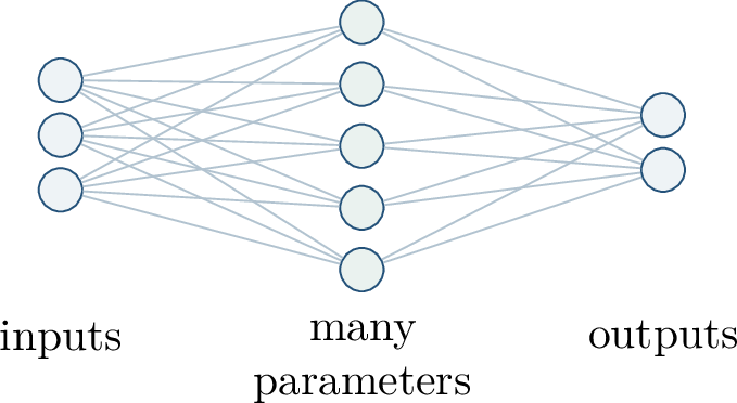
Double descent does not say that larger models always generalize better. It says that the classical U-shape is incomplete once interpolation is possible. The curve depends on noise, signal strength, features, optimizer, and regularization. Stability and double descent are complementary lenses, not a single universal theory.
3.0.15 Limitations and Further Directions↩︎
The main thread of the chapter is \[\text{replace one point} \Rightarrow \text{small algorithmic change} \Rightarrow \text{small generalization gap}.\] Average stability exactly equals expected generalization. Uniform stability turns this identity into cleaner expected and high-probability guarantees. Strong convexity, explicit weight decay, and SGD dynamics provide mechanisms for stability. Differential privacy gives a stronger output-distribution notion of single-sample influence. Double descent shows why pure capacity-based intuition is incomplete in interpolating regimes.
There are also important limits. Uniform stability can be too strong for modern nonconvex networks. Stability bounds may not explain all sharp empirical differences in generalization. Privacy guarantees often require noise that hurts accuracy. Double descent is cleanest in solvable models, whereas deep networks also learn representations. A major open direction is to combine stability with geometry, margins, compression, PAC-Bayes analysis, and implicit-bias theory.
Chapter Synthesis This chapter developed stability as an algorithmic route to generalization. Average stability is exactly the expected generalization gap, while uniform stability gives cleaner expected and high-probability guarantees by controlling the effect of replacing one example. Strong convexity and Lipschitzness make ERM stable because curvature limits movement of the minimizer and Lipschitzness converts movement into loss change. Explicit regularization creates such curvature, while SGD can be stable through a dynamical coupling controlled by step sizes and training time. Differential privacy is a related, stronger output-distribution sensitivity notion. Finally, double descent shows that interpolation changes the classical bias-variance picture: risk can spike near the interpolation threshold and then decrease again when a benign interpolator, such as the minimum-norm solution, is selected.
This chapter is based on the Chapter 6 Beamer source folder for stability, regularization, and double descent, together with the scanned reference note 408lec6post.pdf. Key background works include Bousquet and Elisseeff on stability [14], Hardt, Recht, and Singer on SGD stability [15], Belkin et al. on the modern double-descent viewpoint [16], and Hastie, Montanari, Rosset,
and Tibshirani on high-dimensional ridgeless least squares [36]. Differential privacy and high-probability stability are discussed
here at the level used in the chapter and provide useful bridges to modern algorithm-dependent generalization theory.
3.0.16 From Double Descent to Learnability↩︎
The preceding chapter introduced double descent as a modern replacement for the simple U-shaped bias–variance story. This chapter has two connected goals. First, we complete an exact calculation for ridgeless linear regression, the cleanest model in which the interpolation peak and the second descent can be seen algebraically. Second, we turn from statistical phenomena to computational questions: even if a class can represent a good predictor and has reasonable sample complexity, can it be learned by an efficient algorithm?
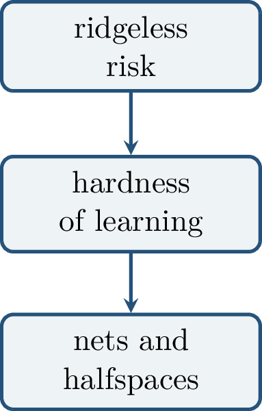
The organizing question is not merely whether a class is expressive. A useful theory of deep learning must keep at least four lenses in view: approximation and representation, optimization, generalization, and computation. The first three lenses appeared repeatedly in earlier chapters. The fourth becomes unavoidable when a theorem says that a good network exists but gives no efficient way to find it, or when a training problem is computationally hard even though the class is statistically learnable.
The two halves of the chapter are connected by the same warning: existence is not enough. In ridgeless regression, the existence of many interpolators does not determine the risk until an algorithmic selection rule, such as minimum norm, is specified. In learning theory, the existence of a small target formula does not determine learnability until the learner’s output class and runtime are specified. Both stories ask what the training procedure is allowed to select.
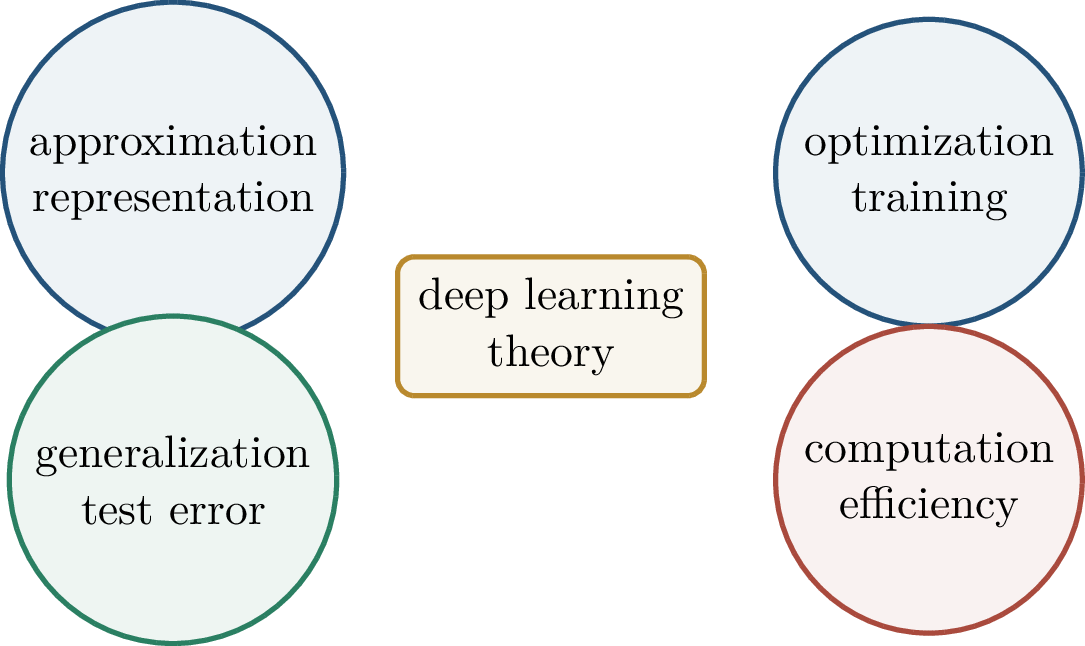
Double descent already warns us that a one-dimensional notion of model size can be misleading. In classical bias–variance reasoning, increasing capacity reduces approximation error but raises estimation variance. In interpolating models, the test risk can spike near the interpolation threshold and then decrease again in an overparameterized regime.
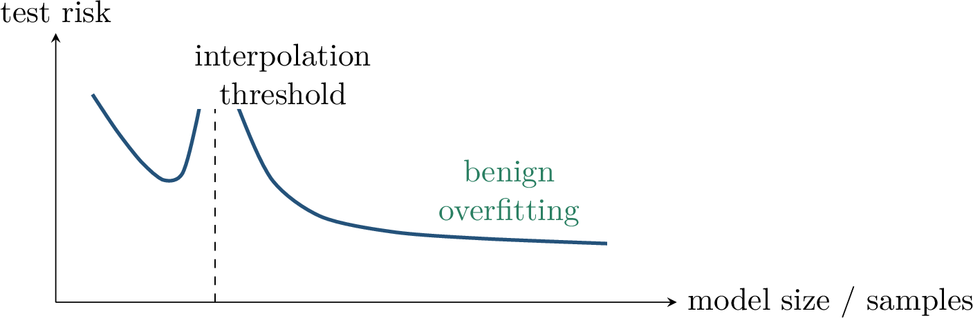
The first part of the chapter asks where this curve comes from in a solvable model. The second part asks a different question: if a nonlinear class is powerful enough to interpolate, is there an efficient learner that can exploit it?
This shift is important for interpreting overparameterization. A larger model can make interpolation easy, but it may also enlarge the statistical search space. Conversely, a larger output representation can make an otherwise hard proper-learning problem algorithmically easy. The rest of the chapter makes these tradeoffs concrete in two settings: Gaussian linear regression and Boolean concept classes.
3.0.17 Ridgeless Risk Decomposition↩︎
We begin with the linear teacher model \[y = X\beta+\varepsilon,\qquad \E[\varepsilon\mid X]=0,\qquad \Cov(\varepsilon\mid X)=\sigma^2 I_n,\] where \(X\in\R^{n\times p}\) has rows \(x_i^\top\). The parameter \(\beta\in\R^p\) is fixed, while the labels contain noise \(\varepsilon\). Let \[\widehat\Sigma=\frac{1}{n}X^\top X.\] The ridgeless least-squares estimator is the minimum Euclidean norm solution among all least-squares minimizers: \[\widehat\beta = \argmin_{b\in \argmin_u \left\lVert y-Xu \right\rVert_2^2}\left\lVert b \right\rVert_2 = (X^\top X)^+X^\top y.\] When \(p>n\) and \(X\) has full row rank, this is the minimum-norm interpolator \(X\widehat\beta=y\). When \(p<n\) and the least-squares solution is unique, it is the usual ordinary least-squares estimator.
The Moore–Penrose pseudoinverse is doing two different jobs in the two regimes. When \(p<n\), it solves an overdetermined least-squares problem. When \(p>n\), it chooses one point from the affine solution set \(\{b:Xb=y\}\), namely the one with smallest Euclidean norm. Thus the same formula encodes both ordinary least squares and the implicit bias of gradient descent from the origin in an underdetermined linear system.
For a test point with covariance matrix \(\Sigma\), define the prediction norm \[\left\lVert b \right\rVert_{\Sigma}^2=b^\top\Sigma b.\] Conditioning on the design matrix \(X\), the prediction risk is \[R(\widehat\beta,\beta) = \E_x\!\left[ \left(x^\top\widehat\beta-x^\top\beta\right)^2 \mid X \right].\] The remaining randomness in \(\widehat\beta\) comes from the label noise.
Conditioning on \(X\), \[R(\widehat\beta,\beta) = B(\widehat\beta,\beta)+V(\widehat\beta,\beta),\] where \[B(\widehat\beta,\beta) = \left\lVert \E[\widehat\beta\mid X]-\beta \right\rVert_{\Sigma}^{2}, \qquad V(\widehat\beta,\beta) = \operatorname{Tr}\!\left[\Cov(\widehat\beta\mid X)\Sigma\right].\]
This is the ordinary bias–variance identity, but written in the prediction geometry induced by \(\Sigma\). The bias term measures the deterministic part of the error left by the algorithm after averaging out label noise; the variance term measures how much the estimator fluctuates because the sample noise is amplified by the design.
Conditioning on \(X\) is what makes the calculation transparent. The rows of \(X\) decide which directions of \(\beta\) are visible and how much noise is amplified. Once \(X\) is fixed, the only remaining randomness is the label noise \(\varepsilon\), so the usual bias–variance decomposition can be applied directly to the random vector \(\widehat\beta\).
Let \[\Pi=I-\widehat\Sigma^+\widehat\Sigma .\] Then \(\Pi\) is the orthogonal projector onto the nullspace of \(X\), and \[B(\widehat\beta,\beta) = \beta^\top\Pi\Sigma\Pi\beta, \qquad V(\widehat\beta,\beta) = \frac{\sigma^2}{n}\operatorname{Tr}\!\left(\widehat\Sigma^+\Sigma\right).\]
Proof. Using \(y=X\beta+\varepsilon\), \[\begin{align} \widehat\beta &=(X^\top X)^+X^\top(X\beta+\varepsilon),\\ \E[\widehat\beta\mid X] &=(X^\top X)^+X^\top X\beta =\widehat\Sigma^+\widehat\Sigma\beta . \end{align}\] Thus \[\begin{align} B(\widehat\beta,\beta) &= \left\lVert (\widehat\Sigma^+\widehat\Sigma-I)\beta \right\rVert_{\Sigma}^{2}\\ &= \left\lVert \Pi\beta \right\rVert_{\Sigma}^{2} = \beta^\top\Pi\Sigma\Pi\beta . \end{align}\] For the covariance, the Moore–Penrose identities give \[\begin{align} \Cov(\widehat\beta\mid X) &= (X^\top X)^+X^\top \sigma^2I_n X(X^\top X)^+\\ &= \sigma^2(X^\top X)^+ = \frac{\sigma^2}{n}\widehat\Sigma^+ . \end{align}\] Substituting this expression into the variance formula gives the stated closed form. ◻
The proposition isolates the two mechanisms behind the ridgeless curve. The bias is the part of the teacher vector that lies in directions unseen by the training design. The variance is an inverse-eigenvalue quantity; it becomes large when the empirical covariance has small nonzero eigenvalues.
This separation is the algebraic heart of the double-descent calculation. In the overparameterized regime, the estimator can interpolate the noisy labels, but interpolation happens only inside the row span of \(X\). Any component of \(\beta\) in the nullspace is not learned and contributes bias. Meanwhile, noise along directions with tiny empirical eigenvalues is amplified by the pseudoinverse and contributes variance.
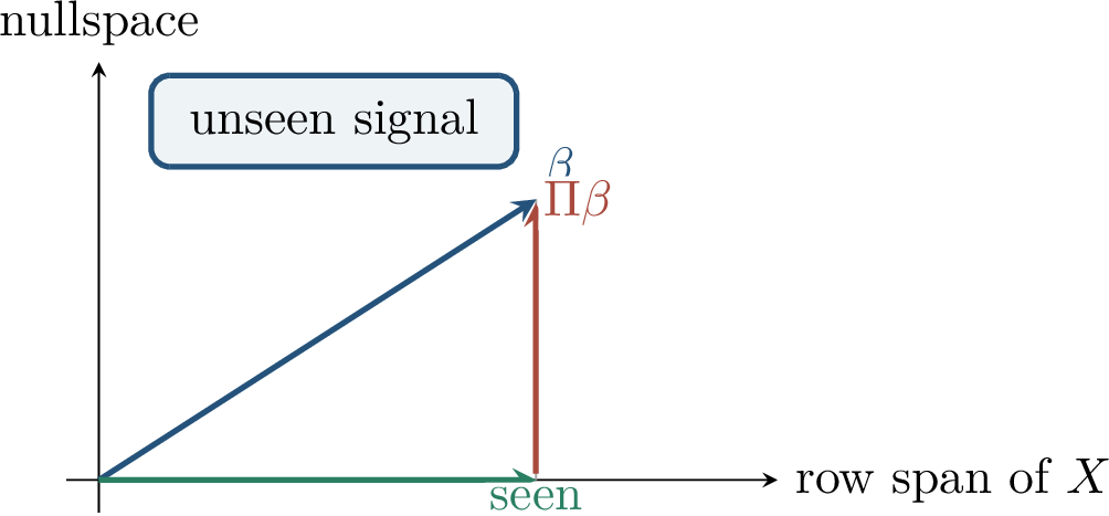
3.0.17.1 Isotropic Gaussian Designs
The formulas become explicit for isotropic Gaussian features. Suppose \[x_i\sim N(0,I_p),\qquad \Sigma=I_p,\qquad \gamma=\frac{p}{n},\qquad \left\lVert \beta \right\rVert_2=r.\] Rotational invariance says that \(X\) and \(XU\) have the same distribution for every orthogonal \(U\). Therefore the row span of \(X\), when it has dimension \(n<p\), is a uniformly random \(n\)-dimensional subspace of \(\R^p\). A fixed direction \(\beta\) contributes an expected fraction \(n/p\) of its squared length to that row span and the remaining fraction to the nullspace. Consequently, \[\E B(\widehat\beta,\beta) = \begin{cases} 0, & 0<\gamma<1,\\[3pt] r^2\left(1-\dfrac{1}{\gamma}\right), & \gamma>1. \end{cases}\] The underparameterized regime has no nullspace bias when \(X\) has full column rank. The overparameterized regime has a nullspace, but as \(\gamma\) grows the variance can decrease even though the bias rises toward the null predictor risk \(r^2\).
The calculation uses only geometry. A uniformly random \(n\)-dimensional subspace captures, on average, the fraction \(n/p\) of the squared length of any fixed vector. Therefore its orthogonal complement captures the remaining fraction \(1-n/p=1-1/\gamma\). This explains why the overparameterized bias depends on \(\gamma\) but not on the particular direction of \(\beta\) in the isotropic model.
For the variance, let \(\lambda_i\) be the nonzero eigenvalues of \(\widehat\Sigma\). Since \(\Sigma=I_p\), \[V(\widehat\beta,\beta) = \frac{\sigma^2}{n}\sum_{\lambda_i>0}\frac{1}{\lambda_i}.\] The inverse eigenvalues are the source of the interpolation spike: near \(\gamma=1\), the smallest nonzero eigenvalues approach zero.
This is the spectral version of instability at interpolation. When \(p\) is close to \(n\), the design matrix is nearly singular. To fit the labels exactly, the pseudoinverse must divide by very small singular values, which amplifies the noise. Once \(p\) is well above \(n\), the nonzero part of the spectrum moves away from this near-singular threshold, and the variance term can decrease again.

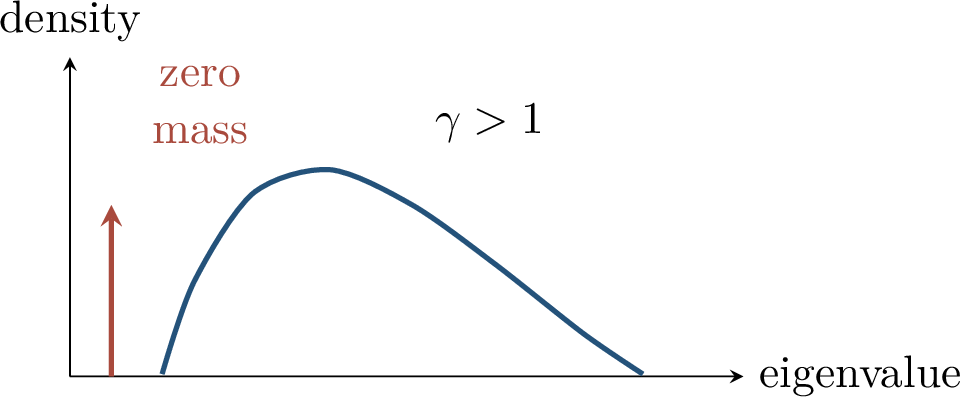
The reference notes emphasize another useful viewpoint. The Stieltjes transform \[\operatorname{Tr}\!\left[ \left(\frac{X^\top X}{n}-zI\right)^{-1} \right] = \sum_i\frac{1}{\lambda_i-z}\] packages the inverse moments of the sample spectrum. Closed forms for this transform under Marchenko–Pastur asymptotics can be evaluated as \(z\to0\), which yields \[V(\widehat\beta,\beta) \approx \begin{cases} \displaystyle \sigma^2\frac{\gamma}{1-\gamma}, &0<\gamma<1,\\[6pt] \displaystyle \sigma^2\frac{1}{\gamma-1}, &\gamma>1. \end{cases}\]
Theorem 0.20 (High-dimensional ridgeless risk, isotropic case). Assume isotropic Gaussian features, \(\Sigma=I_p\), \(\left\lVert \beta \right\rVert_2=r\), and \(p/n\to\gamma\in(0,\infty)\). Away from the interpolation point \(\gamma=1\), the ridgeless prediction risk converges to \[R(\widehat\beta,\beta) \to \begin{cases} \displaystyle \sigma^2\frac{\gamma}{1-\gamma}, &0<\gamma<1,\\[8pt] \displaystyle r^2\left(1-\frac{1}{\gamma}\right) + \sigma^2\frac{1}{\gamma-1}, &\gamma>1. \end{cases}\]
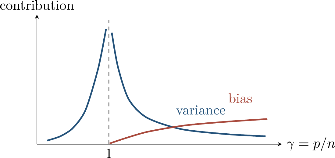
This exact calculation is deliberately special: Gaussian linear features make the spectrum and nullspace geometry tractable. Its value is conceptual. It shows how interpolation can coexist with nontrivial test performance, and it separates the roles of the algorithm’s implicit bias and the sample spectrum. For the rigorous asymptotic analysis of this ridgeless model, see the work of Hastie, Montanari, Rosset, and Tibshirani [36].
3.0.18 Hardness and the Learning Model↩︎
The ridgeless calculation is a positive statistical result. It says that a particular estimator can have interpretable risk in a high-dimensional regime. It does not say that every expressive nonlinear class has an efficient learner. To ask that question we need to specify not only the class and distribution, but also the learning model and the allowed output representation.
This section uses the language of PAC learning. The emphasis is not on sharp sample-complexity constants, but on the distinction between statistical possibility and computational feasibility. A class may have a small description and may even be learnable with polynomially many samples, while the search problem faced by a restricted learner remains computationally hard.
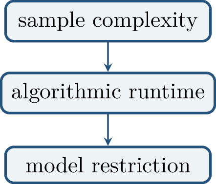
Theorem 0.21 (Blum–Rivest, informal). For a depth-two threshold network with three computational nodes, deciding whether some choice of weights fits all given training examples is NP-hard.
This theorem is striking because the architecture is tiny and fixed; only the weights vary. However, it is a hardness result for a fitting problem with a particular representation requirement. It motivates a careful distinction: is a learner required to output a network from the target class, or is it allowed to output some other efficient predictor that has small error?
Thus the theorem should not be read as saying that all small neural networks are impossible to train in practice. It says that the worst-case consistency problem for a particular threshold-network representation can encode an NP-hard search task. Learning theory therefore asks a more refined question: which output representations are permitted, and what distributional assumptions are being made?
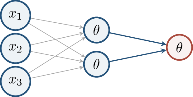
Definition 0.27 (PAC learning benchmark). Let examples \((x,y)\sim\mathcal{D}\) have labels \(y\in\{-1,+1\}\). For a hypothesis \(h:\mathcal{X}\to\{-1,+1\}\), define \[\operatorname{err}_{\mathcal{D}}(h) = \Prob_{(x,y)\sim\mathcal{D}}\!\left[h(x)\ne y\right].\] For a target class \(\mathcal{H}\), the benchmark error is \[\mathrm{OPT}_{\mathcal{H}} = \inf_{h\in\mathcal{H}}\operatorname{err}_{\mathcal{D}}(h).\] A learner competes with \(\mathcal{H}\) if, with high probability over the sample and its internal randomness, it returns \(\widehat h\) satisfying \[\operatorname{err}_{\mathcal{D}}(\widehat h)\le \mathrm{OPT}_{\mathcal{H}}+\varepsilon .\] The usual PAC requirement also asks that the sample size and runtime be polynomial in the natural problem parameters, \(1/\varepsilon\), and \(\log(1/\delta)\).
The benchmark \(\mathrm{OPT}_{\mathcal{H}}\) allows the realizable and agnostic cases to be written in one notation. In the realizable case, some \(h\in\mathcal{H}\) has zero error and \(\mathrm{OPT}_{\mathcal{H}}=0\). In the agnostic case, no member of the class need be perfect, and the learner is asked only to compete with the best member of \(\mathcal{H}\). Computational hardness results can be stated in either setting, but the interpretation depends on which benchmark is used.
Definition 0.28 (Proper and improper learning). A proper learner for \(\mathcal{H}\) must output \(\widehat h\in\mathcal{H}\). An improper learner may output any efficiently evaluable predictor \[\widehat h:\mathcal{X}\to\{-1,+1\},\] as long as it competes with the best member of \(\mathcal{H}\).
The warning is central: hardness of proper learning does not automatically imply hardness of improper learning. A learner may avoid a difficult search inside \(\mathcal{H}\) by moving to a larger representation class \(\mathcal{H}'\).
Improper learning is not a loophole in the definition of learning; it reflects what prediction actually requires. If the goal is small test error, the learner need not recover the same representation that generated the labels. The price is that a larger output class usually requires a stronger generalization argument, because uniform convergence or compression must now control the hypotheses the algorithm might output.
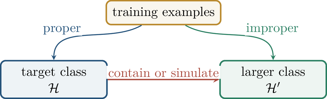
3.0.19 DNF, CNF, and Improper Learning↩︎
Boolean formulas give a clean example of the difference between proper and improper learning. Let each literal be either \(x_j\) or its negation \(\overline{x}_j\).
The point of the example is not that Boolean formulas are themselves neural networks. The point is representational. A concept may have a compact description in one language while being easier to search for in another. The learner can deliberately output a larger or less elegant representation if that representation supports a simple algorithm.
Definition 0.29 (CNF and DNF classes). A \(3\)-CNF formula is a conjunction of clauses with three literals: \[\phi(x) = \bigwedge_{i=1}^{m} (L_{i1}\vee L_{i2}\vee L_{i3}).\] A \(k\)-term DNF formula is a disjunction of \(k\) conjunctions of literals: \[f(x) = \bigvee_{i=1}^{k} \left(\bigwedge_{j=1}^{n_i}L_{ij}\right).\]
Theorem 0.22 (Pitt–Valiant, informal). Unless \(\mathrm{RP}=\mathrm{NP}\), there is no polynomial-time algorithm that properly learns \(k\)-term DNF formulas for \(k\ge3\).
This theorem seems discouraging, but it targets proper learning. The next identity shows why one should be cautious before concluding that the concept class is hopeless.
Proper learning forces the algorithm to return a DNF formula of the same general kind as the target. Improper learning may instead use a related CNF or an expanded DNF-like representation. The algebraic identity below is the mechanism behind this escape: a small DNF can be represented by a structured CNF whose clauses are not arbitrary but are generated by choosing one literal from each term.
Lemma 0.12 (A structured CNF representation). Let \(f=T_1\vee T_2\vee T_3\) be a three-term DNF. Then \[T_1\vee T_2\vee T_3 = \bigwedge_{\substack{L_1\in T_1\\L_2\in T_2\\L_3\in T_3}} (L_1\vee L_2\vee L_3).\]
Proof. If some term, say \(T_1\), is true, then every literal in \(T_1\) is true, so every clause on the right-hand side contains a true literal and is true. Thus the right-hand side is true. Conversely, if \(T_1,T_2,T_3\) are all false, choose one false literal \(L_i\) from each term \(T_i\). The clause \((L_1\vee L_2\vee L_3)\) appears in the displayed conjunction and is false, so the right-hand side is false. ◻
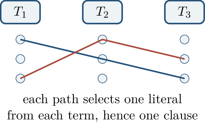
The transformed formula is not an arbitrary \(3\)-CNF. Pitt and Valiant use this special structure to encode hard combinatorial problems for proper learning. But if the learner is allowed to output a larger class, then a simple deletion procedure can succeed.
This is an instructive reversal. The structured CNF may be much larger than the original DNF, but it makes the search monotone: start with all candidate terms and only delete those contradicted by negative examples. The algorithm does not need to guess which target terms are present; it only removes terms that cannot be present.
Theorem 0.23 (Valiant-style improper learning, informal). For constant \(k\), a \(k\)-term DNF can be learned in polynomial time by outputting a hypothesis in a larger CNF/DNF-derived class.
One convenient way to view the algorithm is through complements. The complement of a \(k\)-CNF is a DNF whose terms have \(k\) literals: \[\overline{\bigwedge_i(L_{i1}\vee\cdots\vee L_{ik})} = \bigvee_i (\overline{L}_{i1}\wedge\cdots\wedge\overline{L}_{ik}).\] Thus an algorithm for large DNF classes can be used, after label complementation, to learn the enlarged CNF representation. In the deletion algorithm below, the “target terms” are the \(k\)-literal conjunctions in this complement-view DNF.
Definition 0.30 (Winnow-style deletion algorithm). Let \(S\) initially contain all \(k\)-literal conjunctions over the input variables. Predict \[h_S(x)=\bigvee_{T\in S}T(x).\] Whenever an example has \(h_S(x)=1\) but label \(y=0\), delete from \(S\) every term \(T\) that is true on \(x\). Leave \(S\) unchanged otherwise.
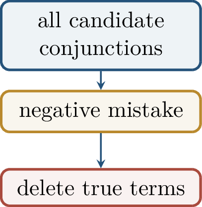
Lemma 0.13 (No false deletions). Suppose a conjunction \(T\) is one of the terms in the target DNF being learned in the complement view. The deletion algorithm never removes \(T\).
Proof. A target term cannot be true on a negative example; if it were true, the target DNF would label the example positive. Since deletion occurs only on negative examples and removes only terms true on that example, a true target term is never deleted. ◻
Lemma 0.14 (Perfect training fit). After processing the sample, the final hypothesis agrees with every training example.
Proof. Negative mistakes are repaired immediately by deleting all currently true terms, so the same processed negative example will not be mislabeled again. For a positive example, at least one true target term is true; by the previous lemma that term remains in \(S\), so the final disjunction labels the example positive. ◻
The price is statistical. Let \(N_k\) be the number of possible \(k\)-literal conjunctions. For constant \(k\), \[N_k\le (2d)^k, \qquad \left\lvert \mathcal{H}' \right\rvert\le 2^{N_k},\] where \(d\) is the number of Boolean variables. For \(k=3\), this gives \(\log\left\lvert \mathcal{H}' \right\rvert=O(d^3)\); the reference notes record the convenient bound \(\left\lvert \mathcal{H}' \right\rvert\le 2^{8d^3}\).
This is exactly the computational–statistical tradeoff promised earlier. The larger improper class makes the algorithm easy because deletion is local and monotone. But the generalization proof must pay for the number of hypotheses in that larger class. For constant \(k\), the logarithm of the class size is still polynomial in \(d\), so the tradeoff remains efficient.
Lemma 0.15 (Finite-class generalization bound). Let \(\mathcal{H}'\) be finite and let \(M\) be the sample size. With probability at least \(1-\delta\), every \(h\in\mathcal{H}'\) satisfies \[\operatorname{err}_{\mathcal{D}}(h) \le \operatorname{err}_S(h) + \sqrt{ \frac{\log\left\lvert \mathcal{H}' \right\rvert+\log(1/\delta)}{2M} }.\]
The deletion algorithm returns a training-consistent hypothesis in \(\mathcal{H}'\), so the finite-class bound gives generalization once \(M\) is large enough relative to \(\log\left\lvert \mathcal{H}' \right\rvert\). The moral is the main point of this example: improper learning can turn a computational barrier into a statistical cost.
The finite-class bound is intentionally crude but sufficient. It does not use any special distributional structure of the Boolean cube, nor does it exploit the fact that the deletion algorithm returns a very particular element of \(\mathcal{H}'\). The purpose is to show, with the simplest possible generalization argument, how a polynomial-time improper learner can exist even when proper learning is hard.
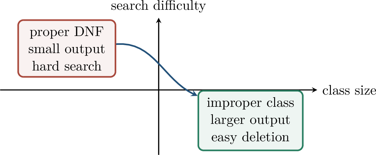
3.0.20 Neural Networks, Halfspaces, and Cryptographic Hardness↩︎
The DNF example prevents a common mistake: proper hardness alone is not a representation-independent lower bound. For neural networks, the analogous question is whether a hard training problem might become easy if the learner can output a different efficient predictor. The next result says that, for some classes related to threshold networks, even improper learning is hard under cryptographic assumptions.
This is the point where the lesson becomes stronger. For DNF, proper hardness did not prevent an improper learner. For the halfspace-intersection class below, the hardness statement allows the learner to output any efficient predictor. The obstruction is no longer merely that the target representation is inconvenient; it is that successful prediction would break an assumed-hard cryptographic task.
Definition 0.31 (Halfspace and intersection of halfspaces). A halfspace classifier is \[h_{w,b}(x)=\sign(\left\langle w,x \right\rangle-b).\] An intersection of \(m\) halfspaces is the Boolean function \[f(x)=1 \quad\Longleftrightarrow\quad h_j(x)=1 \;\text{for every } j=1,\ldots,m.\]
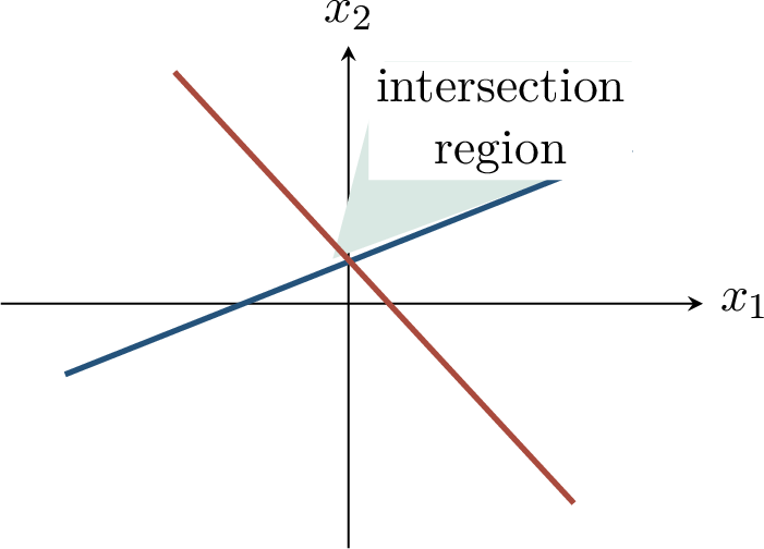
Threshold activations are halfspace tests. If hidden units output \(g_j(x)\in\{-1,+1\}\), then the AND of \(m\) such tests can be written as a single threshold gate: \[F(x) = \sign\!\left(\sum_{j=1}^m g_j(x)-(m-1)\right).\] Indeed, if all \(g_j(x)=1\), the argument is \(1\); if at least one hidden unit outputs \(-1\), the argument is at most \(-1\). Thus intersections of halfspaces form a special class of depth-two threshold networks.
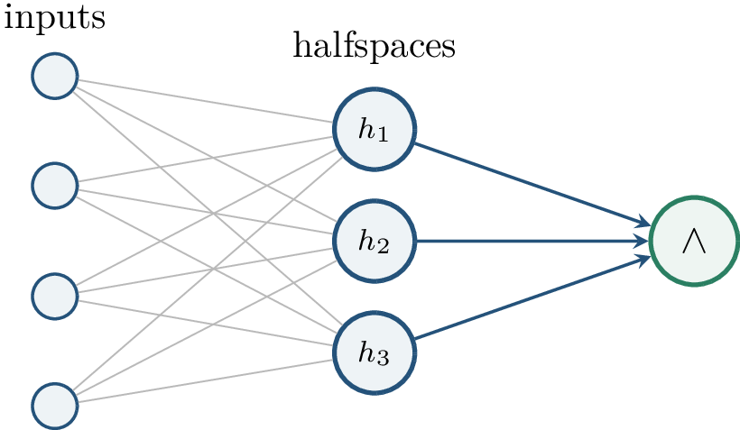
Theorem 0.24 (Klivans–Sherstov, informal). For every constant \(\epsilon>0\), under lattice-based cryptographic assumptions, it is computationally hard to improperly learn intersections of \(n^\epsilon\) halfspaces. Consequently, the corresponding class of depth-two threshold networks is also hard to learn improperly.
This is a stronger message than proper-training hardness. The learner is not required to output halfspaces, or even a neural network. It may output any efficient predictor. The barrier is tied to the prediction task itself under a particular hard distribution.
The theorem is stated informally because the formal result requires specifying the distribution family, the cryptographic assumption, and the precise success criterion. For the purposes of this monograph, the important distinction is that the lower bound is improper: enlarging the output class does not remove the computational barrier under the assumed hardness of the underlying lattice problem.
Definition 0.32 (Lattice and shortest vector problem). A lattice generated by basis vectors \(b_1,\ldots,b_d\) is \[\Lambda = \left\{ \sum_{i=1}^{d}z_i b_i: z_i\in\mathbb{Z} \right\}.\] The shortest vector problem asks for a shortest nonzero vector in \(\Lambda\). The hardness assumption used in this line of work concerns approximating this problem in high dimension.

The reduction idea follows a standard cryptographic template. In a public-key encryption system, an attacker can generate labeled examples by choosing a message \(m\), computing a ciphertext \(x=\operatorname{Enc}(m)\), and labeling it by the decryption value \(y=\operatorname{Dec}(x)=m\). If the decryption rule belongs to the target class and an efficient improper learner could learn it, the attacker would predict decryptions of fresh ciphertexts better than random guessing, contradicting the security of the scheme. Klivans and Sherstov use a Regev-type cryptosystem whose decryption function can be represented as an intersection of \(n^\epsilon\) halfspaces.
The reduction is a bridge from cryptography to learning theory. A secure encryption scheme says that ciphertexts should hide the message from any efficient adversary. A learner that predicts the decryption label from ciphertexts would be exactly such an adversary. Therefore the security assumption rules out the learner. The learning lower bound is only as strong as the cryptographic assumption and the distribution generated by the scheme.
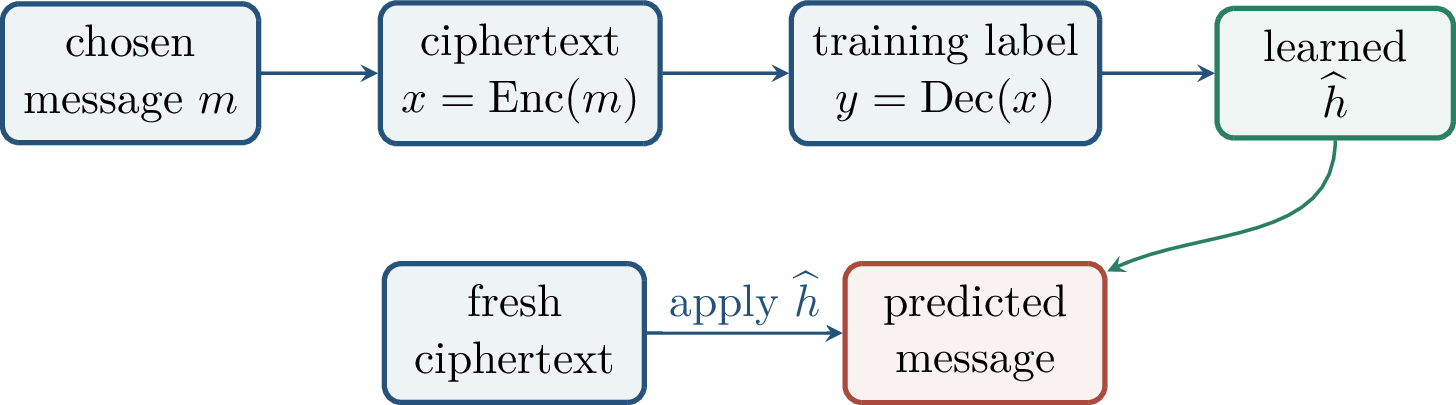
The hard distribution in this theorem is not a natural image or language distribution. It is produced by encrypted random messages. Thus the theorem does not say that practical neural networks cannot be learned; it says that without assumptions on the data distribution, expressive threshold-network classes can encode cryptographically hard prediction problems.
This caveat is essential. Distribution-free lower bounds protect us from overly optimistic universal claims, but they do not replace the study of natural data distributions. Practical success may rely on structure that is absent from the cryptographic construction: smoothness, low-dimensional features, compositionality, invariances, or pretraining-induced representations.
3.0.21 Limits and Further Directions↩︎
The results in this chapter should be read as a map of tradeoffs, not as a single universal verdict.
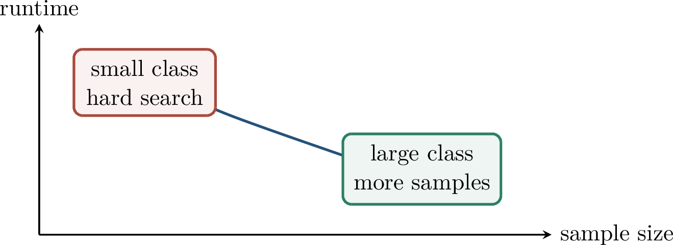
Proper hardness can disappear under improper learning, as the DNF example shows. Cryptographic hardness can survive improper learning, but it may rely on artificial distributions. Average-case assumptions, product or Gaussian input distributions, smoothed models, generative models for data, and algorithmic restrictions such as statistical query access can all change the answer. In practical deep learning, architecture, data structure, optimization bias, and representation learning matter as much as the raw definition of the hypothesis class.
The conceptual bridge back to double descent is this: overparameterization can make optimization easier and can even improve test risk in some regimes, but it can also make classical uniform bounds looser. Improper learning makes the same tension explicit in a different language. A larger class may be easier to search, while demanding more samples for statistical control.
Chapter Synthesis This chapter connected two forms of tradeoff. In ridgeless linear regression, the minimum-norm interpolator has risk that decomposes into nullspace bias and inverse-eigenvalue variance. Isotropic Gaussian designs make this calculation explicit and show why risk can spike near \(p/n=1\) and then decrease on the overparameterized side. The second half of the chapter moved from statistical risk to efficient learnability. Proper learning restricts the output to the target class, while improper learning allows a different representation. DNF/CNF examples show that improper learning can trade a harder search problem for a larger output class and a larger generalization cost. Cryptographic hardness for intersections of halfspaces shows that, under stronger assumptions and artificial distributions, even improper learning can be hard.
This chapter is based on the Chapter 7 Beamer source folder on double descent and improper learning, together with the scanned reference note 408lec7post.pdf. Key background includes the ridgeless-regression analysis of Hastie, Montanari,
Rosset, and Tibshirani [36]. For the computational-learning side, the chapter draws on the classical PAC-learning and hardness
tradition around Blum–Rivest, Valiant, Pitt–Valiant, Littlestone, Kearns–Valiant, Klivans–Sherstov, and Regev. For a related formal model of algorithmic restrictions in learning theory, see Kearns’ work on statistical queries [37].
3.0.22 The Distributional Pivot↩︎
Worst-case learning theory often gives discouraging answers for classes that look quite simple from the point of view of neural networks. Even learning intersections of a small number of halfspaces can be hard if the examples are chosen from an arbitrary distribution. The point of this chapter is not to deny these hardness results, but to ask a different question: what if the input distribution is simple enough that the geometry of the concept becomes visible?
The two distributions emphasized in this chapter are the uniform distribution on the Boolean hypercube and the standard Gaussian distribution. Both have large symmetry groups, strong concentration behavior, and orthogonal bases that convert learning into the estimation of structured statistics. Over the hypercube, the relevant coordinates are the Fourier coefficients of Boolean functions. Over Gaussian space, related ideas appear through Hermite polynomials, anti-concentration, and dimension reduction.
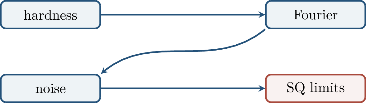
This is the central pivot. In the worst-case setting, difficult examples may hide in rare or adversarial regions. Under a product distribution such as \(\operatorname{Unif}(\{\pm1\}^d)\), a stable boundary cannot be too tangled without revealing itself through high-degree Fourier mass. If most of the function’s energy is in low-degree coefficients, then a learner can estimate those coefficients from samples and build a low-degree polynomial predictor.

The same translation dictionary will be used repeatedly. Geometry of a decision boundary determines its sensitivity to random perturbations. Noise sensitivity controls the high-degree Fourier tail. A small Fourier tail gives a low-degree learning algorithm. In the opposite direction, parity functions hide all of their mass in a single high-degree coefficient, making them almost invisible to algorithms that only ask for coarse averages.
This is also why the chapter belongs in a theory of deep learning. Many neural-network procedures can be interpreted as searching for useful low-complexity statistics of the data distribution: correlations, margins, moments, gradients, and stable features. Fourier analysis gives a clean mathematical language for such statistics in the Boolean case. It separates two questions that are often conflated: whether a simple predictor exists, and whether the learning procedure has access to the statistics that identify it.
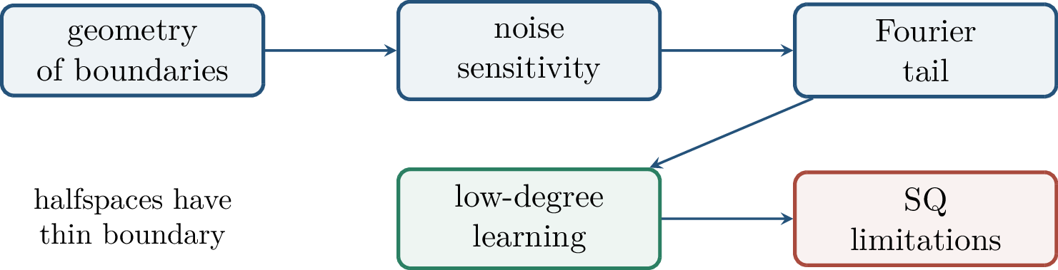
3.0.23 Fourier Analysis on the Hypercube↩︎
We work first on the Boolean hypercube \[\{\pm1\}^d=\{-1,+1\}^d\] with the uniform distribution. A typical example is \(x=(x_1,\ldots,x_d)\sim\operatorname{Unif}(\{\pm1\}^d)\), and the label is \(y=f(x)\), where often \(f:\{\pm1\}^d\to\{\pm1\}\). For a Boolean hypothesis \(h\), the classification error under the same distribution is \[\operatorname{err}(h) = \Prob_{x\sim\operatorname{Unif}(\{\pm1\}^d)}\!\left[h(x)\ne f(x)\right].\] The uniform measure is not chosen only for convenience. It makes the coordinate signs independent and mean zero, so products of coordinates become orthogonal test functions. The resulting theory is the Boolean analogue of expanding a function on an interval into sines and cosines; here the basic waves are parity functions rather than trigonometric functions. We will use only the elementary parts of this theory, but the standard reference for a systematic treatment is [38].
The hypercube has a natural orthonormal basis indexed by subsets of coordinates.
Definition 0.33 (Parity characters). For \(S\subseteq[d]\), the parity character \(\chi_S\) is \[\chi_S(x)=\prod_{i\in S}x_i, \qquad \chi_\emptyset(x)=1.\] Its degree is \(\left\lvert S \right\rvert\). The characters multiply according to \[\chi_S(x)\chi_T(x)=\chi_{S\triangle T}(x),\] where \(S\triangle T\) is the symmetric difference.
The name “parity” is literal: after converting signs into bits, \(\chi_S\) records whether the selected coordinates have even or odd parity. Low-degree characters depend on only a few coordinates, while high-degree characters are global interactions.
Example 0.5 (First Fourier coordinates). For \(d=2\), every real-valued function on \(\{\pm1\}^2\) has the form \[f(x_1,x_2) = a_\emptyset +a_{\{1\}}x_1 +a_{\{2\}}x_2 +a_{\{1,2\}}x_1x_2 .\] The constant coefficient \(a_\emptyset\) is the average value of \(f\). The linear coefficients measure correlation with the individual coordinates, and the degree-two coefficient measures the residual interaction that is visible only after looking at the product \(x_1x_2\). In higher dimension, degree plays the same role: it records how many coordinates must be coupled to see a given feature.
Every function \(f:\{\pm1\}^d\to\R\) has a unique expansion \[f(x)=\sum_{S\subseteq[d]}\widehat f(S)\chi_S(x), \qquad \widehat f(S)=\E_x\!\left[f(x)\chi_S(x)\right],\] where the expectation is over \(x\sim\operatorname{Unif}(\{\pm1\}^d)\). With inner product \(\left\langle f,g \right\rangle=\E_x[f(x)g(x)]\), the family \(\{\chi_S:S\subseteq[d]\}\) is orthonormal.
The orthogonality check is a one-line calculation. If \(S\ne T\), then \(S\triangle T\ne\emptyset\), so choose \(j\in S\triangle T\). Independence and \(\E[x_j]=0\) give \[\begin{align} \E_x[\chi_S(x)\chi_T(x)] &= \E_x[\chi_{S\triangle T}(x)]\\ &= \E[x_j]\, \prod_{i\in S\triangle T,\;i\ne j}\E[x_i] = 0. \end{align}\] When \(S=T\), the product is identically \(1\).
The coefficient \(\widehat f(S)\) should therefore be read as a correlation: it is large precisely when \(f(x)\) tends to align with the parity pattern \(\chi_S(x)\). This interpretation is useful algorithmically because a correlation is an expectation and can be estimated from samples. It is also useful conceptually because it tells us what information a low-degree algorithm is allowed to see: only correlations with parities depending on a small number of coordinates.
Theorem 0.25 (Parseval identity). For every \(f:\{\pm1\}^d\to\R\), \[\E_x[f(x)^2]=\sum_{S\subseteq[d]}\widehat f(S)^2.\] In particular, if \(f(x)\in\{\pm1\}\), then \(\sum_S\widehat f(S)^2=1\).
Proof. Expand both copies of \(f\) in the Fourier basis: \[\begin{align} \E[f(x)^2] &= \E\!\left[ \left(\sum_S\widehat f(S)\chi_S(x)\right) \left(\sum_T\widehat f(T)\chi_T(x)\right) \right]\\ &= \sum_{S,T}\widehat f(S)\widehat f(T) \E[\chi_S(x)\chi_T(x)]. \end{align}\] Orthonormality removes every cross term with \(S\ne T\), leaving \(\sum_S\widehat f(S)^2\). ◻
Parseval lets us treat the squared \(L_2\) norm of a function as the total energy of its Fourier spectrum. The central algorithmic question becomes: is most of the energy visible at low degree?
For Boolean \(f\), the total energy equals one. Hence a spectral concentration statement is a quantitative statement about where this unit energy lives. If most of it is at degrees \(0,1,\ldots,k\), then \(f\) is well approximated by a degree-\(k\) polynomial under the uniform distribution. If most of it sits at degree close to \(d\), then a low-degree polynomial sees very little of the target, even though the function may be perfectly simple from another point of view.
Definition 0.34 (Low-degree truncation). For an integer \(\ell\ge0\), define \[f_{<\ell}(x) = \sum_{\left\lvert S \right\rvert<\ell}\widehat f(S)\chi_S(x).\] This is the orthogonal projection of \(f\) onto the span of characters of degree \(<\ell\).
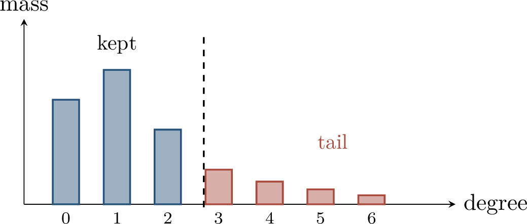
3.0.24 Low-Degree Learning↩︎
Definition 0.35 (Fourier concentration). A function \(f:\{\pm1\}^d\to\R\) is \(\alpha(\epsilon,d)\)-concentrated if \[\sum_{\left\lvert S \right\rvert\ge \alpha(\epsilon,d)}\widehat f(S)^2 \le \epsilon.\] A concept class \(\mathcal{H}\) is \(\alpha(\epsilon,d)\)-concentrated if every \(f\in\mathcal{H}\) has this property.
Fourier concentration is exactly an \(L_2\) approximation statement. If \(g=f_{<\alpha}\), then \[f-g=\sum_{\left\lvert S \right\rvert\ge\alpha}\widehat f(S)\chi_S,\] and Parseval gives \[\E_x[(f(x)-g(x))^2] = \sum_{\left\lvert S \right\rvert\ge\alpha}\widehat f(S)^2.\] Thus the spectral tail is not merely an analogy for the approximation error; it is the approximation error.
Two qualifications are worth making explicit. First, concentration is always relative to the distribution used to define the inner product; changing the distribution changes the notion of orthogonality and can change which features are low degree. Second, concentration is an approximation property, not a representation property of a particular neural network. It tells us that a low-degree polynomial predictor exists under the uniform distribution; additional arguments are needed to explain whether a given training algorithm will find a useful representation.
Theorem 0.26 (Low-degree learning under uniform inputs). Suppose every \(f\in\mathcal{H}\) is \(\alpha(\epsilon,d)\)-concentrated. Then the low-degree Fourier learner learns \(\mathcal{H}\) over \(\operatorname{Unif}(\{\pm1\}^d)\) with runtime \[d^{O(\alpha(\epsilon,d))} \cdot \operatorname{poly}(1/\epsilon,\log(1/\delta)).\] The algorithm estimates all Fourier coefficients of degree \(<\alpha(\epsilon,d)\) and outputs the sign of the resulting polynomial.
This theorem is the Linial–Mansour–Nisan philosophy in a form suited to this principle: spectral concentration implies learnability. The learner does not search over \(\mathcal{H}\). It estimates a universal set of statistics \(\E[y\chi_S(x)]\) for all low-degree parities.
This distinction is important. A proper learner would try to output a member of the original class \(\mathcal{H}\), which may require solving a difficult combinatorial search problem. The low-degree Fourier learner is improper: it outputs the sign of a polynomial assembled from empirical correlations. The price paid for this universality is the number of coefficients. If \(\alpha\) is constant or logarithmic, the method can be meaningful; if \(\alpha\) grows polynomially with \(d\), the enumeration of all subsets \(\left\lvert S \right\rvert<\alpha\) becomes prohibitive.
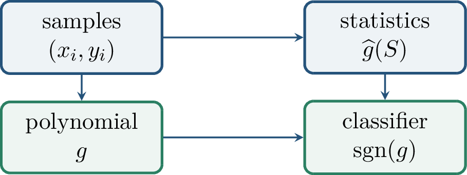
More concretely, for every \(S\subseteq[d]\) with \(\left\lvert S \right\rvert<\alpha\), the learner estimates \[\widehat g(S) = \frac{1}{m}\sum_{i=1}^m y_i\chi_S(x_i).\] It then forms \[g(x)=\sum_{\left\lvert S \right\rvert<\alpha}\widehat g(S)\chi_S(x), \qquad h(x)=\operatorname{sgn}(g(x)).\] There are \[\sum_{j=0}^{\alpha-1}\binom{d}{j} \le d^{O(\alpha)}\] coefficients to estimate.
Lemma 0.16 (Coefficient accuracy implies prediction accuracy). Suppose the estimated low-degree coefficients satisfy \[\sum_{\left\lvert S \right\rvert<\alpha} \left(\widehat g(S)-\widehat f(S)\right)^2 \le \epsilon,\] and suppose \(f\) has Fourier tail mass at most \(\epsilon\) above degree \(\alpha\). Then \[\E_x[(g(x)-f(x))^2]\le 2\epsilon.\]
Proof. The error \(g-f\) has two orthogonal components: coefficient-estimation error inside the low-degree subspace and the ignored high-degree tail. Parseval therefore yields \[\begin{align} \E[(g(x)-f(x))^2] &= \sum_{\left\lvert S \right\rvert<\alpha} \left(\widehat g(S)-\widehat f(S)\right)^2 + \sum_{\left\lvert S \right\rvert\ge\alpha}\widehat f(S)^2\\ &\le 2\epsilon. \end{align}\] ◻
For Boolean labels, \(L_2\) control gives classification control. If \(f(x)\in\{\pm1\}\) and the sign of \(g(x)\) is wrong, then \(\left\lvert f(x)-g(x) \right\rvert\ge1\). Hence \[\mathbf{1}\{\operatorname{sgn}(g(x))\ne f(x)\} \le (f(x)-g(x))^2,\] and therefore \[\Prob[\operatorname{sgn}(g(x))\ne f(x)] \le \E[(f(x)-g(x))^2].\] Hoeffding’s inequality and a union bound over the \(d^{O(\alpha)}\) coefficients show that \[m= \Theta\!\left( \frac{d^{O(\alpha)}}{\epsilon^2} \log\frac{d^{O(\alpha)}}{\delta} \right)\] samples suffice to control all empirical estimates simultaneously with probability at least \(1-\delta\).
The displayed sample bound is deliberately conservative. It is enough for the conceptual theorem because each random variable \(y_i\chi_S(x_i)\) is bounded in \([-1,1]\), and the same argument applies uniformly over all low-degree subsets. More refined analyses can improve constants or avoid estimating coefficients whose empirical mass is negligible, but they do not change the central message: the algorithmic bottleneck is the dimension of the low-degree Fourier subspace.
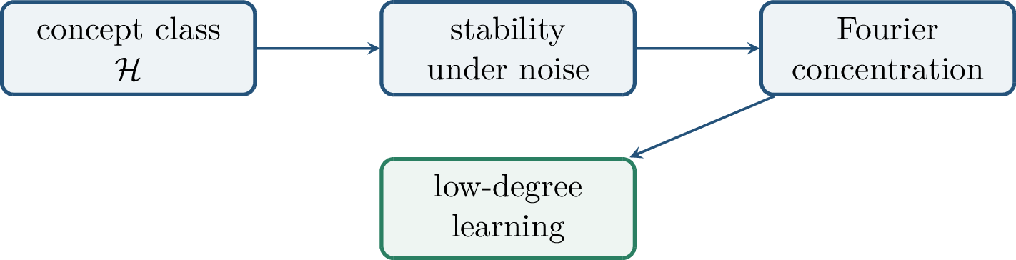
The remainder of the positive part of the chapter explains one powerful way to prove concentration: show that the function is stable under random noise.
3.0.25 Noise Sensitivity and Fourier Tails↩︎
Definition 0.36 (Random bit noise). For \(x\in\{\pm1\}^d\) and \(0\le\eta\le1/2\), let \(T_\eta(x)\) be obtained by flipping each coordinate of \(x\) independently with probability \(\eta\).
Definition 0.37 (Noise sensitivity). For a Boolean function \(f:\{\pm1\}^d\to\{\pm1\}\), define \[\operatorname{NS}_\eta(f) = \Prob_x\!\left[f(x)\ne f(T_\eta(x))\right].\]
Noise sensitivity measures how much of the decision rule is located near a random local boundary. If flipping a small random fraction of coordinates usually preserves the label, then the function has a stable large-scale structure. If the label changes often, then the function depends on delicate high-frequency information. Parity on many coordinates is the extreme example of the second behavior.
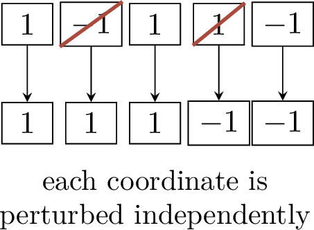
Noise sensitivity has an exact Fourier formula.
For Boolean \(f:\{\pm1\}^d\to\{\pm1\}\) and \(0\le\eta\le1/2\), \[\operatorname{NS}_\eta(f) = \frac{1}{2} - \frac{1}{2} \sum_{S\subseteq[d]}(1-2\eta)^{\left\lvert S \right\rvert}\widehat f(S)^2.\]
Proof. Since \(f(x)f(T_\eta x)=1\) when the labels agree and \(-1\) when they differ, \[\operatorname{NS}_\eta(f) = \frac{1}{2}-\frac{1}{2}\E[f(x)f(T_\eta x)].\] Expanding \(f\) in the Fourier basis and using independence of the coordinate flips gives \[\begin{align} \E[f(x)f(T_\eta x)] &= \sum_{S,U}\widehat f(S)\widehat f(U) \E[\chi_S(x)\chi_U(T_\eta x)]\\ &= \sum_S\widehat f(S)^2 \E[\chi_S(x)\chi_S(T_\eta x)]. \end{align}\] For a fixed coordinate, the product \(x_i(T_\eta x)_i\) equals \(+1\) with probability \(1-\eta\) and \(-1\) with probability \(\eta\), so its expectation is \(1-2\eta\). Multiplying over \(i\in S\) yields \[\E[\chi_S(x)\chi_S(T_\eta x)] = (1-2\eta)^{\left\lvert S \right\rvert}.\] Substitution gives the formula. ◻
The multiplier \((1-2\eta)^k\) is close to \(1\) for small degrees \(k\), but decays rapidly once \(k\gg1/\eta\). Thus noise acts as a low-pass filter on the Fourier spectrum.
Equivalently, the noise operator diagonalizes in the Fourier basis. A degree-\(k\) character survives the perturbation with correlation \((1-2\eta)^k\). This diagonalization is the reason the formula is so useful: probabilistic stability of labels can be converted into an algebraic bound on Fourier coefficients.
Example 0.6 (Dictatorships and parities under noise). For the dictatorship \(f(x)=x_1\), the only nonzero Fourier coefficient is \(\widehat f(\{1\})=1\). The spectral formula gives \[\operatorname{NS}_\eta(f)=\frac{1}{2}\left(1-(1-2\eta)\right)=\eta,\] which is exactly the probability that the first coordinate is flipped. For the parity \(f(x)=\chi_S(x)\), the formula gives \[\operatorname{NS}_\eta(f)=\frac{1}{2}\left(1-(1-2\eta)^{\left\lvert S \right\rvert}\right).\] Thus a high-degree parity becomes unstable even for small \(\eta\), because many coordinates can independently cause a sign change.
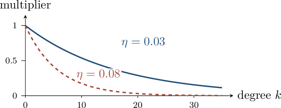
Lemma 0.17 (Stability implies low-degree mass). For \(0<\eta<1/2\) and Boolean \(f\), \[\sum_{\left\lvert S \right\rvert\ge 1/\eta}\widehat f(S)^2 \le \frac{2}{1-e^{-2}}\operatorname{NS}_\eta(f).\]
Proof. By Parseval and the spectral formula, \[\begin{align} 2\operatorname{NS}_\eta(f) &= \sum_S\widehat f(S)^2 \left(1-(1-2\eta)^{\left\lvert S \right\rvert}\right)\\ &\ge \left(1-(1-2\eta)^{1/\eta}\right) \sum_{\left\lvert S \right\rvert\ge1/\eta}\widehat f(S)^2. \end{align}\] Finally, \((1-2\eta)^{1/\eta}\le e^{-2}\), so \(1-(1-2\eta)^{1/\eta}\ge1-e^{-2}\). ◻
This lemma turns a geometric estimate into an algorithmic certificate. If a class satisfies a bound \(\operatorname{NS}_\eta(f)\le B(\eta)\), then one chooses \(\eta\) as a function of the desired error \(\epsilon\), obtains Fourier concentration at degree \(O(1/\eta)\), and runs the low-degree learner.
The constants are less important than the direction of implication. The lemma does not say that every function with small high-degree Fourier mass is geometrically simple, but it does say that every sufficiently noise-stable Boolean function is spectrally simple at an appropriate scale. This one-way bridge is exactly what is needed for learning.
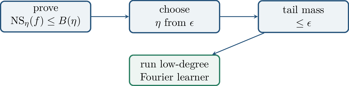
3.0.26 Halfspaces and Intersections↩︎
The main positive example in the chapter is the class of intersections of halfspaces. This class is directly related to simple threshold networks.
Definition 0.38 (Halfspace). A halfspace on the hypercube is a Boolean function \[h(x)=\operatorname{sgn}(\left\langle w,x \right\rangle-\theta), \qquad w\in\R^d,\;\theta\in\R.\]
Definition 0.39 (Intersection of halfspaces). An intersection of \(k\) halfspaces is \[f(x)=\operatorname{AND}(h_1(x),\ldots,h_k(x)),\] where \(f(x)=1\) exactly when all \(k\) threshold tests accept.
This class can be viewed as a depth-two threshold circuit: the first layer computes halfspace features, and the second layer computes their AND.
We will use the sign convention already implicit in the chapter. On a continuous distribution, the exact value at margin zero is irrelevant because the boundary has probability zero. On the finite hypercube, tie points can matter for constants, but the learning mechanism below is controlled by how much mass lies near the threshold, not by the arbitrary naming of a tie.
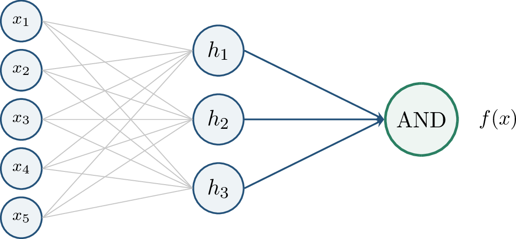
Theorem 0.27 (Peres noise bound). For every halfspace \(h\) and every \(0<\eta<1/2\), \[\operatorname{NS}_\eta(h)\le C\sqrt{\eta}\] for a universal constant \(C\).
The geometric intuition is simple. A noisy point changes the label of a halfspace only if the perturbation carries it across the separating boundary. Under product measure, most mass is not extremely close to any one linear threshold, so only a band of width on the order of \(\sqrt{\eta}\) contributes substantially.
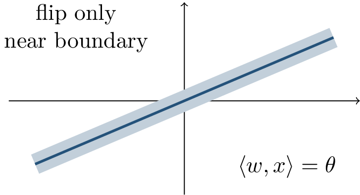
The majority function is the clean mental model. Let \[\operatorname{Maj}(x)=\operatorname{sgn}\!\left(\sum_{i=1}^d x_i\right), \qquad X=\frac{1}{\sqrt d}\sum_{i=1}^d x_i.\] By the central limit theorem, \(X\) is approximately \(N(0,1)\). After random bit noise, the normalized sum changes by a random amount of typical scale \(O(\sqrt{\eta})\). The sign can flip mainly when \(X\) lies in a band of width \(O(\sqrt{\eta})\) around zero. The Gaussian mass of that band is also \(O(\sqrt{\eta})\), matching Peres’s bound.
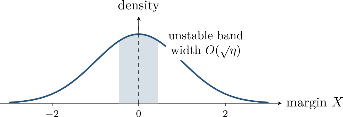
Noise stability is also compositional.
If \[h(x)=g(f_1(x),\ldots,f_k(x)),\] then \[\operatorname{NS}_\eta(h)\le \sum_{i=1}^k \operatorname{NS}_\eta(f_i).\]
Proof. If \(h(x)\ne h(T_\eta x)\), then at least one input bit to \(g\) must change: there exists \(i\) such that \(f_i(x)\ne f_i(T_\eta x)\). Taking probabilities and applying the union bound gives the claim. ◻
Combining Peres’s bound, the union bound, and the stability-to-concentration lemma gives the basic low-degree learning theorem for intersections.
Theorem 0.28 (Klivans–O’Donnell–Servedio learning result, informal). For every constant \(k\), intersections of \(k\) halfspaces are learnable over \(\operatorname{Unif}(\{\pm1\}^d)\) by a low-degree Fourier algorithm. The proof gives the runtime \[d^{O(k^2/\epsilon^2)}\] for error parameter \(\epsilon\), up to polynomial factors for sampling and confidence.
Proof skeleton. Let \(f\) be an intersection of \(k\) halfspaces. By the union bound and Peres’s theorem, \[\operatorname{NS}_\eta(f)\le Ck\sqrt{\eta}.\] The stability lemma then gives \[\sum_{\left\lvert S \right\rvert\ge1/\eta}\widehat f(S)^2 \le \frac{2C}{1-e^{-2}}k\sqrt{\eta}.\] Choosing \(\eta=\Theta(\epsilon^2/k^2)\) makes the Fourier tail at most \(\epsilon\). The low-degree learner therefore needs degree \[\alpha=O(k^2/\epsilon^2),\] which leads to the displayed running time. ◻
The union bound is not the end of the story. For intersections of many halfspaces, Kane proved a sharper noise sensitivity estimate.
Theorem 0.29 (Kane noise bound, informal). For an intersection \(f\) of \(k\) halfspaces, \[\operatorname{NS}_\eta(f)\le C\sqrt{\eta\log k}.\]
Corollary 0.2 (Improved low-degree learning). Using Kane’s bound, the Fourier learner runs in time \[d^{O(\log k/\epsilon^2)}\] over the uniform hypercube.
The improvement is conceptually meaningful even though the algorithm remains super-polynomial when \(k\) grows quickly. The naive union bound treats the \(k\) boundaries as if all their unstable regions were disjoint. Sharper geometric arguments exploit the fact that these regions overlap and that a random perturbation cannot independently cross every boundary at full cost. The result is a logarithmic dependence on \(k\) in the noise bound rather than a linear one.
The reference notes also point to a complementary Gaussian result. For \(x\sim N(0,I_d)\), intersections of halfspaces can be learned more directly by exploiting the low-dimensional span of the normals \[W=\operatorname{span}\{w_1,\ldots,w_k\}.\] Conditioning on positive or negative examples changes variance most strongly in the directions of these normal vectors. Once the span is recovered, learning effectively occurs in dimension \(k\) rather than \(d\). This Gaussian viewpoint uses the same moral as the hypercube argument: a structured distribution turns geometry into learnable statistics.
3.0.27 Statistical Queries↩︎
The positive results above estimate many expectations. This motivates a learning model that abstracts algorithms which only interact with the data through stable averages. The statistical query model was introduced by Kearns as a framework for noise-tolerant learning from approximate expectations [37].
Definition 0.40 (Statistical query model). In the statistical query model, a learner may submit a bounded query \[q:\mathcal{X}\times\mathcal{Y}\to[-1,1]\] and a tolerance \(\tau>0\). The oracle returns a number \(r\) satisfying \[\left| r-\E_{(x,y)\sim\mathcal{D}}[q(x,y)] \right| \le \tau.\] The learner sees approximate expectations, not individual samples.
An SQ algorithm is efficient when it asks at most polynomially many queries, uses inverse-polynomial tolerances, evaluates its queries efficiently, and computes the final hypothesis efficiently. Such an algorithm can be simulated from samples: for a bounded query, the empirical average \[\frac{1}{m}\sum_{i=1}^m q(x_i,y_i)\] approximates \(\E[q(x,y)]\) to tolerance \(\tau\) using \(m=O(\tau^{-2}\log(1/\delta))\) samples for that query.
The tolerance parameter is essential. A query with tolerance \(10^{-3}\) asks for a robust statistic that can be estimated from a moderate number of samples. A query with tolerance \(2^{-d}\) is closer to asking for an exact combinatorial coincidence hidden in the distribution. SQ lower bounds show that some targets are learnable from raw examples but not from any polynomial number of robust aggregate statistics.
The model is powerful enough to include many moment, correlation, and gradient-based procedures. Population gradients in neural-network training, for instance, are expectations: \[\nabla_\theta L(\theta) = \E_{(x,y)} \left[ \nabla_\theta \ell(f_\theta(x),y) \right].\] Mini-batch SGD estimates these expectations. If a useful signal is exponentially small in all such averages, SQ lower bounds suggest a training barrier for this broad family of methods.

3.0.28 Parity Functions and SQ Lower Bounds↩︎
Parity functions are the canonical example separating raw-sample algorithms from statistical-query algorithms.
Definition 0.41 (Unknown parity). Choose an unknown set \(T\subseteq[d]\). Draw \(x\sim\operatorname{Unif}(\{\pm1\}^d)\) and label \[y=\chi_T(x)=\prod_{i\in T}x_i.\]
The Fourier spectrum of this target is concentrated on exactly one coefficient, namely \(T\). If \(T\) is large, the target is high degree and very noise sensitive. This is the opposite of the low-degree situation: there is no broad low-degree signature to estimate.
This example is deliberately unforgiving. A single parity is not complicated to describe once \(T\) is known, but the identity of \(T\) is a high-degree combinatorial secret. The target therefore exposes a weakness of algorithms that rely only on averaged correlations: unless a query has been aligned with the hidden subset, its expectation gives essentially no information.
Theorem 0.30 (BFJKMR lower bound for parity, informal). Any statistical query algorithm that learns arbitrary parity functions on \(\{\pm1\}^d\) must either make exponentially many queries or use exponentially small tolerance.
Here is the Fourier intuition behind the lower bound. It is enough to focus on correlational queries of the form \[q(x,y)=yq_0(x).\] If \(y=\chi_T(x)\) and \[q_0(x)=\sum_{S\subseteq[d]}\widehat q_0(S)\chi_S(x),\] then \[\E[yq_0(x)] = \E[\chi_T(x)q_0(x)] = \widehat q_0(T).\] The oracle response therefore reveals whether the query has noticeable Fourier mass at the hidden set \(T\).
But a bounded query cannot have large Fourier mass in too many places. Parseval gives \[\sum_S \widehat q_0(S)^2 = \E[q_0(x)^2] \le 1.\] Consequently, at most \(1/\tau^2\) subsets \(S\) can satisfy \[\left\lvert \widehat q_0(S) \right\rvert\ge\tau.\] If \(\left\lvert \widehat q_0(T) \right\rvert<\tau\), the SQ oracle may answer zero. Since there are \(2^d\) possible hidden parities, one query can noticeably test only a \(\tau^{-2}\)-sized portion of the possibilities. Roughly \(2^d\tau^2\) queries are needed unless \(\tau\) is exponentially small.
The argument above is only an intuition for the full BFJKMR theorem, because general SQ queries need not be simple correlational queries. The full lower bound formalizes the same idea using statistical dimension: a large family of nearly uncorrelated targets cannot be distinguished by a small number of coarse expectation queries. For the purposes of this chapter, the Fourier calculation captures the reason parity is the canonical obstruction.
The contrast with raw samples is sharp.
Without label noise, an unknown parity can be learned in polynomial time from raw labeled examples by solving a linear system over \(\mathbb{F}_2\).
Proof. Write \(x_j=(-1)^{z_j}\) with \(z_j\in\mathbb{F}_2\), and represent the hidden set \(T\) by a vector \(c\in\mathbb{F}_2^d\). Then \[\chi_T(x)=(-1)^{c\cdot z}.\] If \(y=(-1)^b\), the labeled example gives the linear equation \[c\cdot z=b \pmod 2.\] Stacking the equations from the sample gives \(Ac=b\pmod2\). Gaussian elimination over \(\mathbb{F}_2\) recovers \(c\) once the examples span the relevant directions. ◻
Noisy parity is different again. If each label is flipped independently with a constant probability below \(1/2\), the exact linear-system trick becomes non-robust. The Blum–Kalai–Wasserman algorithm learns noisy parity in subexponential time \[2^{O(d/\log d)},\] which is far faster than brute force but still far from polynomial. Noisy parity remains a central benchmark for average-case learning lower bounds.
Chapter Synthesis
Distributional assumptions can turn geometric regularity into learnable statistics; over the Boolean hypercube, those statistics are Fourier coefficients.
Parseval’s identity makes Fourier tail mass exactly equal to low-degree \(L_2\) approximation error.
Low-degree concentration yields an improper learner obtained by estimating low-degree correlations and thresholding the resulting polynomial.
Noise sensitivity provides a bridge from boundary geometry to Fourier concentration, with halfspaces and intersections of halfspaces as the main positive examples.
Statistical queries model algorithms that see approximate expectations; parity functions show that such access can miss exact high-degree information visible in raw samples.
3.0.29 What the Chapter Adds↩︎
This chapter gives both a positive and a negative lesson.
On the positive side, distributional assumptions can reveal useful low-degree structure. Under the uniform distribution, Fourier analysis converts learning into coefficient estimation. Noise sensitivity supplies a geometric route to Fourier concentration. Halfspaces are stable, intersections inherit enough stability, and low-degree algorithms follow.
On the negative side, not all information is visible to coarse statistics. Parity functions hide the target in one high-degree Fourier coefficient. SQ queries can only detect a limited number of possible high-degree directions at any fixed tolerance, even though raw samples solve noiseless parity by linear algebra. This distinction matters for deep learning theory because many training signals, including population gradients, are expectations.
Several limitations should be kept in view.
Fourier concentration over the hypercube is distribution dependent; it need not transfer to arbitrary data distributions.
Low-degree algorithms such as \(d^{O(1/\epsilon^2)}\) can be too slow to explain the practical efficiency of modern neural networks.
Agnostic versions often aim for \(\mathrm{OPT}+\epsilon\), but the constants and runtime dependencies are important.
Existence of a low-degree predictor does not by itself explain how a trained neural network finds a comparable representation.
SQ lower bounds identify barriers for robust-statistic algorithms, not for every possible raw-sample method.
The next stage of the monograph will continue this theme: compare what neural network training can do under structured distributions, especially Gaussian inputs, with what is possible under statistical-query access.
This chapter is based on the Chapter 8 Beamer source folder 408lec8_distributional_fourier_sq and the scanned reference note 408lec8post.pdf. For background on Boolean Fourier analysis and noise sensitivity, see [38]; for the statistical query framework, see [37]. The main sources and themes are the Linial–Mansour–Nisan low-degree learning principle, Peres’s noise sensitivity bound for halfspaces, the Klivans–O’Donnell–Servedio result for
intersections of halfspaces, Kane’s improved noise bound, the Blum–Furst–Jackson–Kearns–Mansour–Rudich SQ lower bound for parity, and the Blum–Kalai–Wasserman noisy-parity algorithm.
3.0.30 Why SGD Lower Bounds Are Subtle↩︎
The previous chapter introduced statistical queries as a model for algorithms that interact with data through stable expectations. This chapter asks how far that model can explain barriers for gradient-based training. The guiding principle is simple: \[\text{SQ hardness} \quad\Longleftrightarrow\quad \text{weak gradient signal}.\] If every useful gradient coordinate is an exponentially small correlation, then algorithms that can only estimate such correlations need exponentially many queries or exponentially high precision.
There is an important caveat. Ordinary mini-batch SGD sees individual samples through its stochastic updates. Raw samples can contain exact combinatorial information, as parity learning already demonstrated. The lower bounds in this chapter therefore apply most cleanly to noisy population gradient descent, or to training procedures whose update law can be coupled to a CSQ simulation. This distinction is not pedantic; it is the difference between a statistical limitation and an unconditional computational lower bound.
Throughout the chapter we will keep this distinction visible. An oracle lower bound says that a certain information channel is too weak: if an algorithm receives only approximate correlations, then it cannot identify the target efficiently. A lower bound for a concrete training algorithm requires an additional simulation step showing that the algorithm’s trajectory can be reproduced from that weak channel. The noisy-gradient coupling below is precisely such a simulation step.
We will use three algorithmic lenses. An SQ algorithm asks for approximate expectations \(\E[q(x,y)]\pm\tau\). A CSQ algorithm is more restrictive: it only asks for label correlations \(\E[y\phi(x)]\pm\tau\). Noisy population gradient descent updates parameters by following the population gradient and then adding independent Gaussian noise.
The restriction from SQ to CSQ matters because a CSQ oracle is aligned with the form of squared-loss gradients. In a gradient coordinate, the label appears linearly as \(y\) multiplied by a feature depending on \(x\) and the current parameters. General SQ access would allow more complicated statistics involving \(y\), while CSQ access captures the specific correlational information that the gradient requests.

The transfer from parity to Gaussian neural networks goes through orthogonality. Parity functions are hard for CSQ algorithms because a query can correlate noticeably with only a small number of possible hidden parities. For Gaussian shallow networks, the construction embeds a parity-like sign pattern inside a real-valued one-hidden-layer network. Gaussian sign symmetry then supplies pairwise orthogonality.
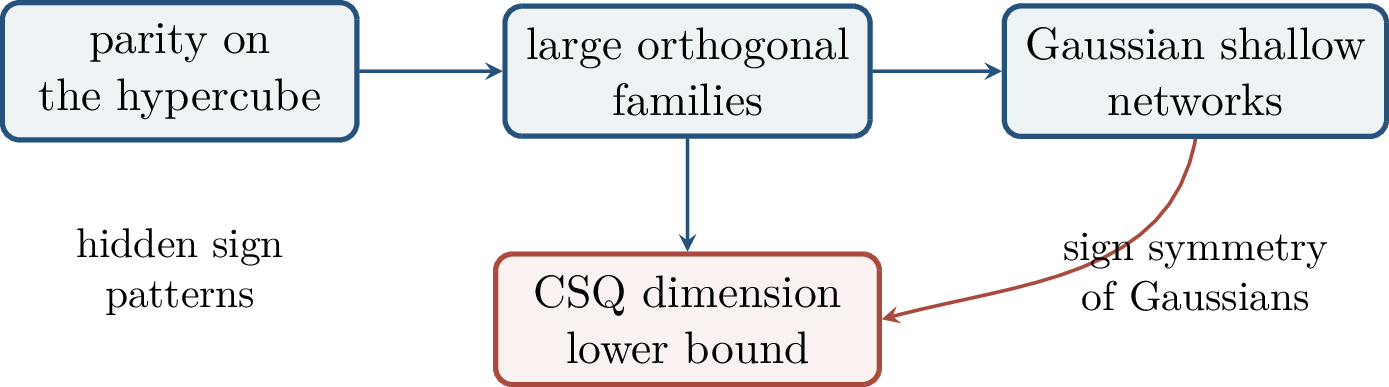
3.0.31 Noisy Gradient Descent as CSQ↩︎
Let \(h_\theta:\R^d\to\R\) be a differentiable model with parameters \(\theta\in\R^p\). For a data distribution \(\mathcal{D}\) on \((x,y)\), define the population squared risk \[R(\theta) = \E_{(x,y)\sim\mathcal{D}}\!\left[(h_\theta(x)-y)^2\right].\] Noisy population gradient descent uses the update \[\theta_{t+1} = \theta_t-\eta\nabla R(\theta_t)+\xi_t, \qquad \xi_t\sim\mathcal{N}(0,s^2I_p),\] where \(s\) is the noise scale. The noise is an algorithmic smoothing parameter, not label noise.
The adjective “population” is also important. The update uses the exact gradient of \(R\), not a mini-batch estimate. In practice one usually observes stochastic gradients from finite samples, but the population model isolates the information contained in the expected update direction. Adding Gaussian noise then makes it possible to compare two nearby update distributions by total variation distance.
Definition 0.42 (Correlational statistical query oracle). A CSQ oracle receives a bounded query \(\phi:\R^d\to[-1,1]\) and a tolerance \(\tau>0\), and returns a number \[v=\E[y\phi(x)]\pm\tau .\] Thus labels are observed only through correlations with functions of \(x\).
This is the correlational part of the statistical query model introduced by Kearns [37]. The boundedness condition is not a technical decoration: it ensures that a query can be estimated from samples at a rate controlled by its tolerance. When a gradient-coordinate function is not naturally bounded by one, the simulation normalizes it and pays the corresponding scale factor in the tolerance.
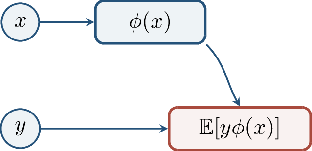
The connection to gradients is direct.
Assume the marginal distribution of \(x\) is known and that the relevant gradient-coordinate functions are bounded after normalization. Each coordinate of \(\nabla R(\theta)\) can be approximated using a known marginal expectation and one CSQ.
Proof. Differentiate under the expectation: \[\begin{align} \nabla_\theta R(\theta) &= \E\!\left[ 2(h_\theta(x)-y)\nabla_\theta h_\theta(x) \right]\\ &= 2\E\!\left[h_\theta(x)\nabla_\theta h_\theta(x)\right] - 2\E\!\left[y\nabla_\theta h_\theta(x)\right]. \end{align}\] The first expectation depends only on the known marginal law of \(x\) and the current parameter vector. The second is a vector of label correlations, one for each coordinate of the gradient. ◻
Thus the only unknown part of the population gradient, once the marginal law of \(x\) is known, is a collection of CSQ answers. The known marginal term can be computed analytically for simple Gaussian models, or treated as free information in the lower-bound reduction. This convention strengthens the learner, so a lower bound under this convention is more convincing.
A CSQ simulation of noisy GD therefore follows the same template at every step: compute the marginal term, estimate the label-correlation term by CSQs, form an approximate gradient, add Gaussian noise, and update.
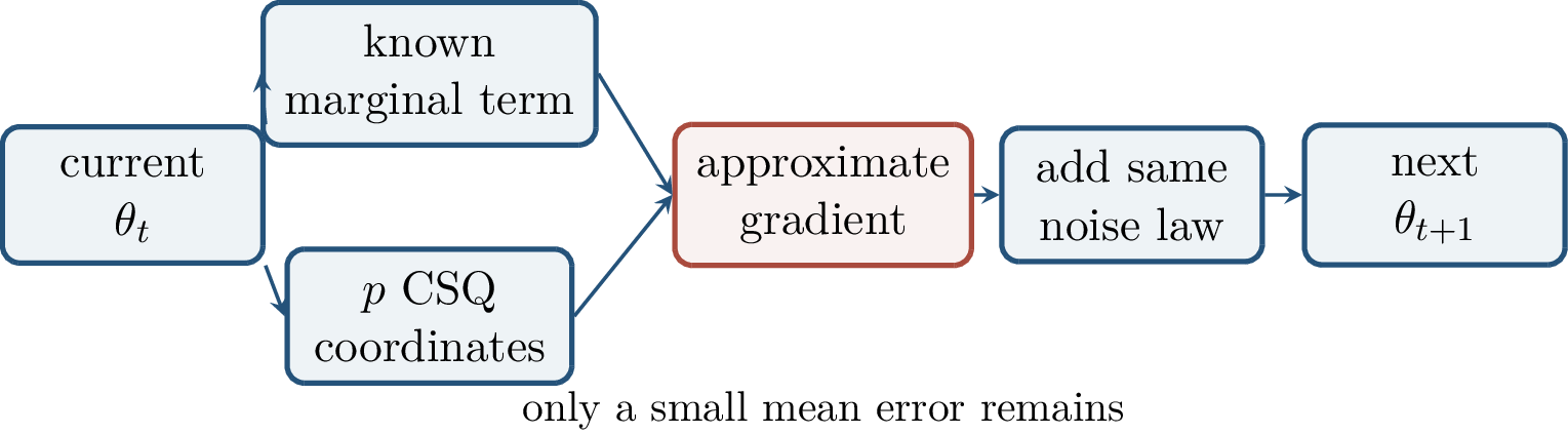
The simulation is distributional rather than pointwise: we want the noisy update produced by the CSQ simulation to agree with the noisy GD update with high probability under a suitable coupling.
The reason for using a coupling is that the two algorithms may not compute the same deterministic vector. They only need to generate nearly the same distribution over the next parameter value. If two one-step transition laws are close in total variation, a maximal coupling realizes them as equal with high probability. Iterating this construction turns a one-step approximation into a trajectory-level approximation.
Definition 0.43 (Coupling). A coupling of random variables \(X\sim\mu\) and \(Y\sim\nu\) is a joint distribution \(\pi\) whose marginals are \(\mu\) and \(\nu\).
If \(\mu\) and \(\nu\) have densities \(f\) and \(g\), the maximum agreement probability over all couplings is \[\int \min\{f(x),g(x)\}\,dx = 1-d_{\mathrm{TV}}(\mu,\nu).\] Moreover, for \[P=\mathcal{N}(\mu,s^2I_p), \qquad Q=\mathcal{N}(\mu',s^2I_p),\] \[d_{\mathrm{TV}}(P,Q) \le \sqrt{\frac{1}{2}D_{\mathrm{KL}}(P\Vert Q)} = \frac{\left\lVert \mu-\mu' \right\rVert_2}{2s}.\]
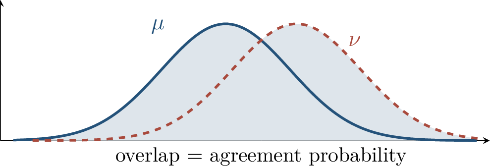
Theorem 0.31 (Noisy GD can be coupled to CSQ). Assume the marginal law of \(x\) is known. A \(T\)-step noisy population GD trajectory in parameter dimension \(p\) can be simulated by a CSQ algorithm with total coupling failure probability at most \(\delta\), using tolerance \[\tau = O\!\left(\frac{\delta s}{T\sqrt p}\right),\] up to normalization constants for the gradient-coordinate queries.
Proof idea. If every gradient coordinate is estimated to accuracy \(\tau\), then the Euclidean error in the mean of the Gaussian update is at most \[\left\lVert \widehat{\nabla R(\theta)}-\nabla R(\theta) \right\rVert_2 \lesssim \sqrt p\,\tau.\] The two one-step update distributions are Gaussians with covariance \(s^2I_p\) and means separated by this amount, so the Gaussian shift bound gives one-step coupling failure probability \(O(\sqrt p\,\tau/s)\). Choosing \(\tau=O(\delta s/(T\sqrt p))\) and applying a union bound over \(T\) steps gives total failure at most \(\delta\). On the success event, the simulated and true parameter vectors are identical at every step. ◻
This proof also explains the role of the noise scale \(s\). Larger injected noise makes nearby mean vectors harder to distinguish, so coarser CSQ tolerances suffice for simulation. If \(s\) is exponentially small, however, the simulation requires exponentially fine CSQ tolerances, and the lower-bound statement becomes correspondingly weaker. This is why the corollary below has two escape routes: either many steps or extremely small injected noise.
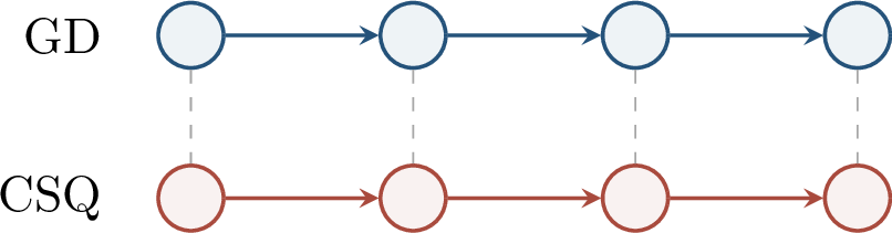
Corollary 0.3 (Parity lower bound transfers). For parity functions under the uniform distribution, any noisy GD method captured by the coupling theorem must either take \[T=\exp(\Omega(d)) \qquad\text{or}\qquad s=\exp(-\Omega(d)),\] up to polynomial factors in the model size and parameter dimension.
The message is not that every form of SGD is weak. It is that noisy population GD, whose informative part is a vector of label correlations, inherits CSQ lower bounds. Ordinary SGD is harder to lower-bound because it can exploit individual samples and numerical precision. In fact, work of Abbe and Sandon shows that, with appropriate constructions and initialization, polynomial-time SGD can simulate arbitrary polynomial-time sample-based algorithms. Strong unconditional lower bounds against such general SGD would therefore imply major complexity separations.
For a reader thinking about practical training, the safest interpretation is therefore conditional. SQ and CSQ lower bounds identify a real obstruction for methods whose progress is driven by robust averages. They do not exclude algorithms that exploit sample-level algebraic structure, finite-precision effects, special initialization, or architecture-specific computation. Much of modern lower-bound work consists of making this modeling boundary explicit.
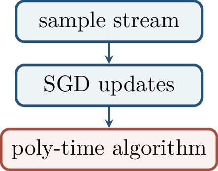

3.0.32 CSQ Lower Bounds for Shallow Networks↩︎
We now move from parity functions to shallow neural networks under Gaussian inputs. Consider one-hidden-layer functions of the form \[f(x) = \sum_{i=1}^m a_i\,\sigma(w_i^\top x), \qquad x\sim\mathcal{N}(0,I_d),\] where \(w_i\in\R^d\) and \(a_i\in\R\). Gaussian inputs make rotations and sign flips exploitable. The signs of the output weights \(a_i\) will be crucial: lower-bound constructions use cancellation, while several positive algorithms rely on nonnegative output weights.
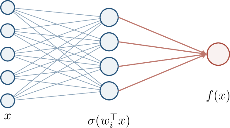
Theorem 0.32 (Informal CSQ lower bound under Gaussians). For common activations such as sigmoid or ReLU, any CSQ algorithm learning one-hidden-layer networks under \(x\sim\mathcal{N}(0,I_d)\) requires either \[d^{\Omega(\log m)} \quad\text{queries} \qquad\text{or}\qquad \tau=d^{-\Omega(\log m)}.\]
The lower bound follows from a CSQ dimension principle.
Theorem 0.33 (CSQ dimension principle, informal). Suppose a class contains \(\ell\) functions \(g_1,\ldots,g_\ell\) such that \[\E_D[g_i(x)g_j(x)]=0\quad(i\ne j), \qquad \E_D[g_i(x)^2]\ge \alpha.\] Then a CSQ learner that reaches error below a constant fraction of \(\alpha\) must use either many queries, on the order of the size of the orthogonal family, or very small tolerance.
The intuition is the same as for parity. A query direction can have noticeable correlation with only a few orthogonal targets. A large orthogonal family forces the learner either to probe many directions or to estimate correlations with extremely high precision.
One can view this as an application of Bessel’s inequality. If a bounded query has inner products \(\left\langle \phi,g_i \right\rangle\) with many orthogonal targets, then \[\sum_i \frac{\left\langle \phi,g_i \right\rangle^2}{\left\lVert g_i \right\rVert_2^2} \le \left\lVert \phi \right\rVert_2^2 .\] Therefore only a limited number of targets can have correlation larger than a fixed tolerance. A single CSQ answer rules out only a small part of a large orthogonal family, so many queries are needed unless the tolerance is tiny.
For Boolean labels and known marginal \(D_X\), many general SQs can be reduced to label correlations. For real-valued labels this is no longer true: general SQ algorithms may ask nonlinear questions such as \(\E[y^2\phi(x)]\). The lower bound in this part is therefore stated for CSQs, which is the model naturally matched to squared-loss gradients.
This limitation is part of the theorem, not a flaw in the proof. The target functions here are real-valued neural networks, and a learner with arbitrary SQ access might ask statistics that are not gradient-like. The lower bound is designed to speak to first-order training signals rather than to every possible statistical procedure.
3.0.33 The Orthogonal Family↩︎
Let \[r=\lceil \log_2 m\rceil.\] The construction chooses a hidden subset \(S\subseteq[d]\) of size \(r\). The number of possible choices is \[\binom{d}{r} \ge \left(\frac{d}{r}\right)^r = d^{\Omega(\log m)}\] when \(m\) is at most polynomial in \(d\). This is the size of the target family the learner must distinguish.
The choice \(r=\lceil\log_2 m\rceil\) balances two competing requirements. The construction needs \(2^r\) hidden units, so \(r\) cannot be much larger than \(\log m\) if the target is to remain an \(m\)-scale shallow network. At the same time, the number of possible hidden subsets grows like \(\binom dr\), which is already \(d^{\Omega(\log m)}\). This is the source of the superpolynomial family size.
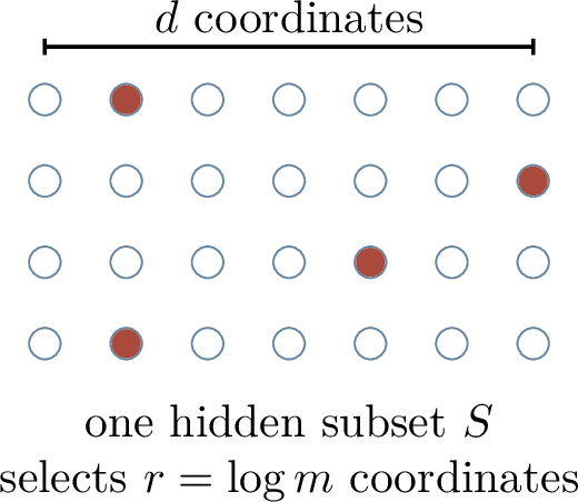
Definition 0.44 (Parity-weighted sigmoid sum). For \(S\subseteq[d]\) with \(\left\lvert S \right\rvert=r\), define \[g_S(x) = \sum_{\omega\in\{\pm1\}^r} \chi(\omega)\, \sigma\!\left(\frac{\omega^\top x_S}{\sqrt r}\right), \qquad \chi(\omega)=\prod_{j=1}^r\omega_j.\] The vector \(x_S\in\R^r\) contains the coordinates of \(x\) indexed by \(S\).
There are \(2^r\le2m\) hidden units in \(g_S\). The output coefficients \(\chi(\omega)\in\{\pm1\}\) create cancellation, while the Gaussian input distribution supplies sign symmetry.
Each summand is a ridge function whose weight vector is supported on the hidden coordinate set \(S\). The learner sees a shallow network of moderate width, but the identity of \(S\) is hidden among many possibilities. The parity signs force the network to respond equivariantly to coordinatewise sign flips, which is what makes different choices of \(S\) orthogonal.
Lemma 0.18 (Parity response to sign flips). For any \(z\in\{\pm1\}^d\) and \(x\in\R^d\), \[g_S(x\circ z)=\chi_S(z)g_S(x), \qquad \chi_S(z)=\prod_{i\in S}z_i.\]
Proof. In the defining sum for \(g_S(x\circ z)\), reindex by \(\omega'=\omega\circ z_S\). The activation arguments match those in \(g_S(x)\), while the parity coefficient changes by the multiplicative factor \(\chi_S(z)\). This gives the displayed identity. ◻
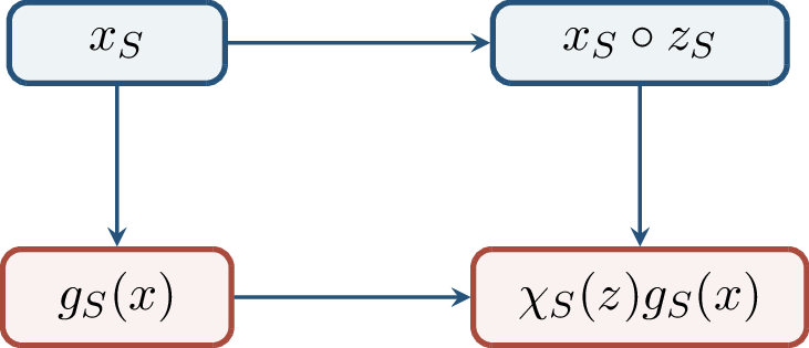
Lemma 0.19 (Pairwise orthogonality). If \(S\ne T\), then \[\E_{x\sim\mathcal{N}(0,I_d)}[g_S(x)g_T(x)]=0.\]
Proof. Let \(z\) be uniformly distributed on \(\{\pm1\}^d\), independent of \(x\). Since a standard Gaussian is invariant under coordinatewise sign flips, \(x\circ z\) has the same distribution as \(x\). Therefore \[\begin{align} \E_x[g_S(x)g_T(x)] &= \E_z\E_x[g_S(x\circ z)g_T(x\circ z)]\\ &= \E_z[\chi_S(z)\chi_T(z)]\, \E_x[g_S(x)g_T(x)]. \end{align}\] If \(S\ne T\), then \(S\triangle T\ne\emptyset\), so \(\E_z[\chi_S(z)\chi_T(z)]=0\). Hence the original expectation must be zero. ◻
Lemma 0.20 (Norm lower bound). For each \(S\) with \(\left\lvert S \right\rvert=\lceil\log_2m\rceil\), \[\E_{x\sim\mathcal{N}(0,I_d)}[g_S(x)^2]\ge m^{-O(1)}\] for standard non-polynomial activations after normalization.
The role of the parity-weighted sum is to isolate a high-order Hermite component of the activation. If \[\sigma(t)=\sum_{k\ge0}\widehat\sigma_k h_k(t)\] is the Hermite expansion, the signed sum over \(\omega\in\{\pm1\}^r\) cancels all monomials that miss at least one selected coordinate. A nonzero high-order coefficient remains, giving nontrivial energy.
This statement should be read with its hypotheses in mind. The activation must have enough non-polynomial content, or at least a nonzero Hermite coefficient at a relevant degree after normalization. The lower-bound construction is not claiming that every activation and every scaling has the same norm lower bound; it uses standard activations precisely because their Hermite expansions retain nontrivial high-order mass.
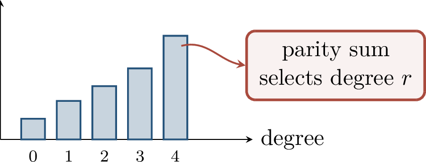
Putting the pieces together, the family \(\{g_S:\left\lvert S \right\rvert=r\}\) has \(\ell=\binom{d}{r}=d^{\Omega(\log m)}\) pairwise orthogonal members, each with nontrivial squared norm. The CSQ dimension theorem then forces superpolynomial CSQ complexity or superpolynomially small tolerance. In a probabilistic concept model where \(x\sim\mathcal{N}(0,I_d)\), \(y\in\{\pm1\}\), and \(\E[y\mid x]=f(x)\), related arguments can yield SQ rather than merely CSQ lower bounds.
The construction is a useful example of how hardness can be embedded into a neural-network class without making individual targets look exotic. Each target is a finite-width one-hidden-layer network. The difficulty lies in the large nearly orthogonal family and in the fact that CSQ access observes only one low-precision correlation at a time.
3.0.34 Landscape Design↩︎
The lower bound construction uses positive and negative output weights to create cancellations. Positive results use different structure. A central example is the reader–teacher setting \[y=f(x)=\sum_{i=1}^m a_i\sigma(w_i^\top x), \qquad x\sim\mathcal{N}(0,I_d),\] where the learner fits \[\widehat y = \sum_{i=1}^m\widehat a_i\sigma(\widehat w_i^\top x).\] The standard squared-loss landscape can contain spurious local minima: it may match low-order moments without recovering the true first-layer weights.
The following Hermite formula explains why moment matching appears at all. Under Gaussian inputs, ridge functions are naturally decomposed by Hermite degree. The \(k\)-th Hermite component of \(\sigma(w^\top x)\) behaves like a rank-one tensor \(w^{\otimes k}\). Training a reader network therefore amounts, at the population level, to matching a weighted sequence of tensor moments of the teacher.
Theorem 0.34 (Hermite tensor moment formula). Assume \(w_i\) and \(\widehat w_i\) are unit vectors and \[\sigma(t)=\sum_{k\ge0}\widehat\sigma_k h_k(t)\] in the normalized Hermite basis. Then the population squared loss can be written as \[L(\widehat a,\widehat W) = \sum_{k\ge0} \widehat\sigma_k^2 \left\| \sum_i \widehat a_i\widehat w_i^{\otimes k} - \sum_i a_iw_i^{\otimes k} \right\|_F^2 +C,\] where \(C\) is independent of the reader parameters.
This identity says that the loss tries to match infinitely many low-rank tensors at once. Different Hermite degrees can pull the parameters in conflicting directions, which explains why the standard objective may be misleading.
For example, a parameter setting may match the degree-two tensor well while misaligning the degree-four tensor, or vice versa. The scalar loss aggregates all of these discrepancies with weights \(\widehat\sigma_k^2\), so a local minimum can reflect a compromise among moments rather than true recovery of the hidden weights.
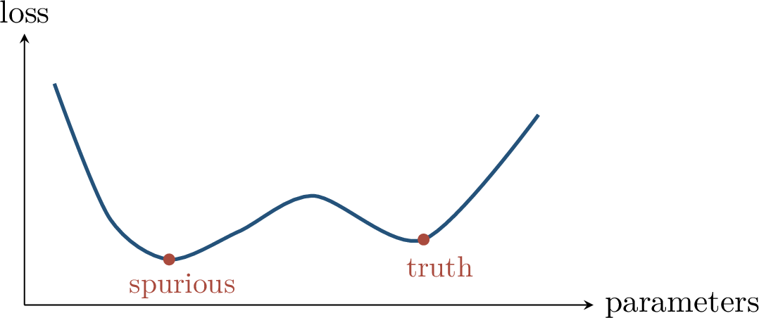
Landscape design changes the objective so that the relevant low-order moment structure has benign critical points.
The design principle is not to make the network more expressive, but to make the objective ask a cleaner question. By filtering the activation to selected Hermite degrees, one suppresses nuisance moment components and emphasizes those that identify the teacher under the structural assumptions.
Definition 0.45 (Hermite-filtered reader). Replace the activation in the reader objective by \[\gamma(t) = \widehat\sigma_2 h_2(t)+\widehat\sigma_4 h_4(t),\] where \[h_2(t)=\frac{t^2-1}{\sqrt2}, \qquad h_4(t)=\frac{t^4-6t^2+3}{\sqrt{24}}.\] Define \[G(\widehat a,\widehat W) = \E\!\left[ \left(\widehat a^\top\gamma(\widehat W x)-y\right)^2 \right].\]
Theorem 0.35 (Informal landscape design guarantee). Under suitable nondegeneracy assumptions and nonnegative output weights \(a_i\ge0\), the designed objective \(G\) has no spurious local minima, its global minima recover the teacher up to symmetry, and its gradients are estimable from samples.
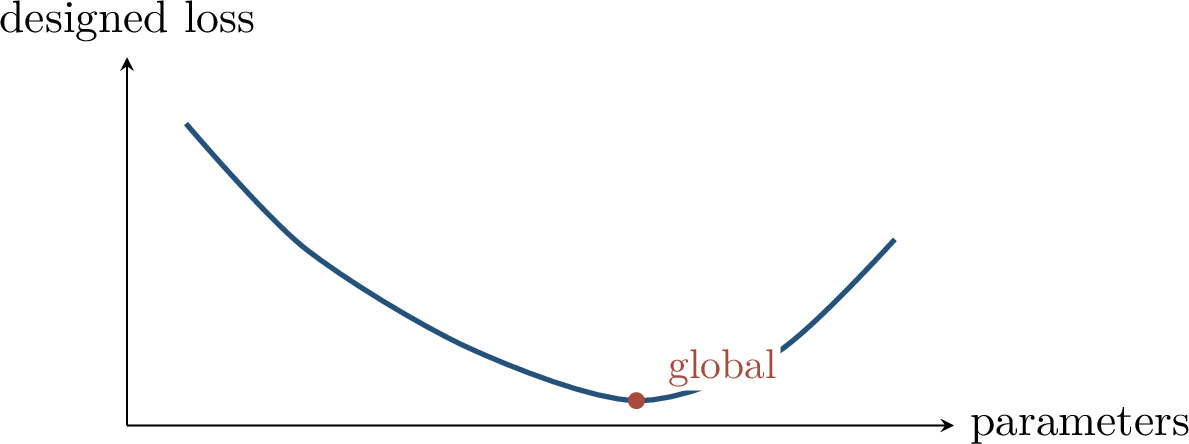
This contrast is a major lesson of the chapter. The CSQ lower-bound family uses \(a_\omega=\chi(\omega)\in\{\pm1\}\), creating parity-like cancellation. When \(a_i\ge0\), large responses point toward the relevant subspace, enabling PCA and designed landscapes. Output-layer signs change the statistical geometry of learning.
This is an example of a broader phenomenon: the same architecture can have very different learnability properties under different sign, distributional, or nondegeneracy assumptions. A lower bound for a cancellation-heavy target family and a positive algorithm for nonnegative mixtures are not contradictory; they illuminate different regions of the model class.
There is also a fixed-parameter tractable viewpoint: for Gaussian inputs, certain ReLU networks can be learned in time \[f(m,\Delta,\epsilon)\,\operatorname{poly}(d),\] where \(m\) measures the number of hidden units and \(\Delta\) controls Lipschitz or norm parameters. The dependence on network parameters may be large, but the dependence on ambient dimension \(d\) is polynomial.
3.0.35 Filtered PCA↩︎
Filtered PCA is a concrete way to exploit the relevant low-dimensional subspace. Let \[V=\operatorname{span}\{w_1,\ldots,w_m\}\] be the span of the teacher weights, and choose a scalar filter \(\psi\). Define the response-weighted covariance \[M_\psi = \E\!\left[\psi(y)(xx^\top-I_d)\right].\] Since \(y=f(x)\) depends only on \(\Pi_Vx\), a suitable filter can make the otherwise isotropic Gaussian distribution anisotropic inside \(V\).
Without the response weight \(\psi(y)\), the covariance of \(x\) is simply \(I_d\), and every direction looks identical. The filter selects examples whose labels reveal something about the active coordinates. After selection, directions in \(V\) can have different second moments from directions in \(V^\perp\), and PCA can detect this anisotropy.
If \(c\perp V\), then \[M_\psi c=0.\]
Proof idea. Write \[x=\Pi_Vx+\Pi_{V^\perp}x.\] The two Gaussian components are independent, and \(y\) depends only on \(\Pi_Vx\). Any factor involving a direction \(c\perp V\) has mean zero after conditioning on \(\Pi_Vx\). Therefore the response-weighted covariance has no action in directions orthogonal to \(V\). ◻
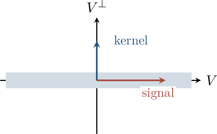
Suppose the filter \(\psi(y)=\mathbf{1}_{\{\left\lvert y \right\rvert\ge\tau\}}\) selects examples for which \[\left\lVert \Pi_Vx \right\rVert^2\ge 2m.\] Then \(M_\psi\) has a positive eigenvalue, and every eigenvector for a positive eigenvalue lies in \(V\).
Proof. Since \(M_\psi\) vanishes on \(V^\perp\), it suffices to show a positive trace on \(V\). Let \(V\) also denote a matrix with orthonormal columns spanning the subspace. Then \[\begin{align} \operatorname{Tr}(V^\top M_\psi V) &= \E\!\left[ \psi(y) \left( \left\lVert \Pi_Vx \right\rVert^2-m \right) \right]. \end{align}\] On the selected event this quantity is at least \(m\), so the trace is positive whenever the event has positive probability. ◻
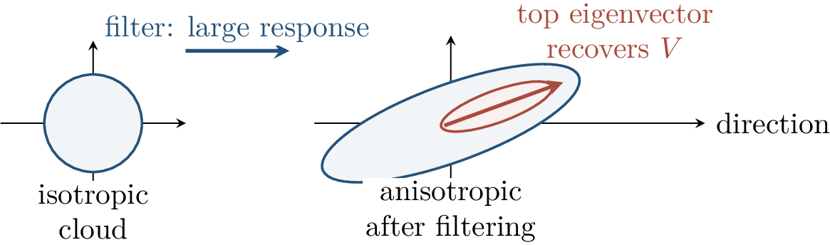
Stein’s lemma explains why second-order response-weighted covariance detects active directions.
Lemma 0.21 (Stein identity). If \(X\sim\mathcal{N}(0,1)\) and \(g\) is sufficiently smooth with suitable decay, then \[\E[g(X)X]=\E[g'(X)].\] Consequently, \[\E[g(X)(X^2-1)]=\E[g''(X)].\]
The second identity is obtained by applying the first identity twice, once to \(g(X)X\) and then simplifying. In multidimensional Gaussian problems, the same integration-by-parts principle relates response-weighted second moments to second derivatives of the target along coordinate directions. This is why the matrix \(M_\psi\) can reveal directions on which the target function actually varies.
Example 0.7 (Quadratic activation). Let \(\sigma(t)=t^2\), let \(V=\operatorname{span}\{e_1,\ldots,e_m\}\), and suppose \(\E[f(x)]=0\). With \(\psi(y)=y^2\), \[\operatorname{Tr}(V^\top M_\psi V) = \sum_{j=1}^m \E\!\left[f(x)^2(x_j^2-1)\right].\] By Stein’s identity, \[\begin{align} \E\!\left[f(x)^2(x_j^2-1)\right] &= \E[\partial_j^2 f(x)^2]\\ &= 2\E[(\partial_j f(x))^2] + 2\E[f(x)\partial_j^2 f(x)]. \end{align}\] For the simple quadratic models in the reference notes, this quantity is positive in active directions, so the top eigenvector of \(M_\psi\) lies in the signal subspace.
The example should not be overread: it is a clean calculation showing the mechanism, not a universal theorem for arbitrary activations. For more general networks, one must choose the filter carefully and control sampling, nondegeneracy, and perturbation errors. The conceptual point remains that Gaussian integration by parts converts derivatives of the teacher into observable anisotropy.
3.0.36 Main Theoretical Consequences↩︎
The same Gaussian structure gives both lower bounds and algorithms. On the negative side, sign symmetry creates large orthogonal families invisible to CSQ algorithms. Noisy population GD, when its gradients are only approximate correlations plus smoothing noise, inherits these CSQ barriers. On the positive side, nonnegative output weights and response filters create detectable anisotropy, and carefully designed objectives can remove spurious local minima in population risk.
The main limitations are equally important. CSQ lower bounds do not rule out all sample-based algorithms. Ordinary SGD can be computationally richer than the SQ abstraction. Positive algorithms often require Gaussian inputs, nonnegative weights, nondegeneracy assumptions, or large fixed-parameter dependence. The open direction is to characterize when the SGD used in practice exploits information beyond stable statistics and when its behavior is accurately predicted by SQ-style reasoning.
Chapter Synthesis
Squared-loss population gradients decompose into a known marginal term and label-correlation queries, so CSQ lower bounds can apply to noisy population gradient methods.
A coupling argument transfers CSQ lower bounds to noisy GD when the injected noise is large enough to hide small gradient-estimation errors.
Shallow-network lower bounds under Gaussian inputs are built from large orthogonal families, using parity-like output signs and Gaussian sign symmetry.
Hermite expansions explain both the lower-bound construction and the landscape-design positive results: Gaussian ridge functions decompose into tensor moments by degree.
Filtered PCA is a positive mechanism: response-weighted covariance can reveal the hidden teacher subspace when structural assumptions prevent cancellation.
This chapter is based on the Chapter 9 Beamer source folder 408lec9_sgd_sq_landscape and the scanned reference note 408lec9post.pdf. Key sources include Moitra’s 18.408 chapter, Abbe–Sandon and Abbe–Kamath–Malach–Sandon–Srebro
on differentiable learning versus PAC/SQ learning, Goel–Gollakota–Jin–Karmalkar–Klivans on gradient-descent lower bounds for one-layer networks, Ge–Lee–Ma on landscape design, Diakonikolas–Kane–Kontonis–Zarifis on algorithms and SQ lower bounds for
one-hidden-layer ReLU networks, and Chen–Klivans–Meka on fixed-parameter tractability for deep ReLU networks.
4 Robustness, Generative Models, and Structured Learning↩︎
4.0.1 An Interlude: Three New Questions↩︎
The reference note for this chapter is explicit: there was no formal theorem chapter on that day, only discussion and a map of the remaining topics. The Beamer source turns that map into an interlude. The first nine chapters focused mostly on supervised learning, optimization, generalization, and distributional assumptions. Chapter 10 shifts the center of gravity. Instead of asking only whether a network fits labels, we ask whether it is reliable under perturbation, whether it can synthesize data, and whether it can make sequential decisions in a feedback loop.
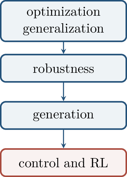
The three themes introduce three new actors. Robustness introduces an attacker. Generative modeling introduces a distributional comparison problem, often represented by a discriminator. Reinforcement learning introduces an environment whose future states depend on the learner’s actions.
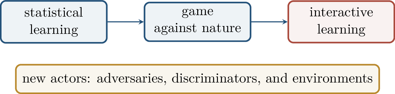
The common pattern is to replace average supervised loss by a stronger notion of success: \[\begin{array}{lll} \text{robustness} &:& \displaystyle \min_f \E\!\left[\max_{\delta\in\Delta} \ell(f(x+\delta),y)\right],\\[5pt] \text{generation} &:& \displaystyle \min_G d(P_{\mathrm{data}},P_G),\\[5pt] \text{reinforcement learning} &:& \displaystyle \max_\pi \E_\pi\!\left[\sum_{t\ge0}\gamma^t r_t\right]. \end{array}\] In all three cases the objective is no longer just a single empirical average over fixed examples. Geometry, dynamics, and model misspecification become part of the mathematical problem.
The word “interlude” should not suggest that these topics are peripheral. They mark a change in what it means for a learned model to succeed. In standard supervised learning, a hypothesis is judged on fresh samples from the same distribution. In robustness, it must behave well in a neighborhood of those samples. In generative modeling, it must represent a distribution rather than a label rule. In reinforcement learning, it must choose actions whose consequences change the future data it will see. The shared theme is that the model is now embedded in a larger system.
4.0.2 Adversarial Robustness↩︎
Definition 0.46 (Adversarial example). For a classifier \(f:\R^d\to\{1,\ldots,k\}\), an adversarial example for \((x,y)\) at radius \(\epsilon\) is a point \[x'=x+\delta, \qquad \left\lVert \delta \right\rVert\le\epsilon, \qquad f(x')\ne y.\] The norm and the radius are part of the robustness specification.
The definition deliberately includes the norm. An \(\ell_\infty\) constraint models many tiny coordinate changes, while an \(\ell_2\) constraint limits the Euclidean size of the perturbation. Neither norm is a perfect model of human perception, but each gives a mathematically explicit threat model. The modern study of adversarial examples began with the observation that very small perturbations can change neural-network predictions [17]; the first-order explanation below follows the linear viewpoint popularized in [39].
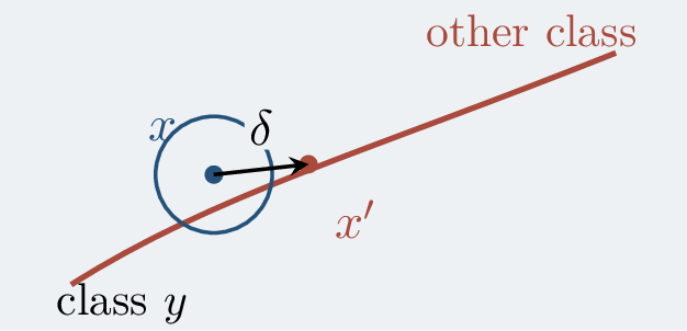
Definition 0.47 (Robust risk). Let \[\Delta_\epsilon=\{\delta:\left\lVert \delta \right\rVert\le\epsilon\}.\] The standard risk and robust risk of a classifier \(f\) are \[R(f)=\Prob[f(X)\ne Y], \qquad R_{\mathrm{rob}}(f) = \Prob\!\left[ \exists\delta\in\Delta_\epsilon: f(X+\delta)\ne Y \right].\] Always \(R(f)\le R_{\mathrm{rob}}(f)\).
Robust risk depends on the geometry of the data distribution, the norm, and the perturbation radius. The local version is a margin notion.
Equivalently, robust risk asks whether the entire perturbation set around a typical input is classified correctly. This is a stronger requirement than standard risk because it quantifies over a continuum of nearby points, many of which may not themselves be natural data samples. The mathematical challenge is therefore partly statistical and partly geometric: the classifier must place its decision boundary away from the data in the metric specified by the threat model.
Definition 0.48 (Local robust radius). For a classifier \(f\), define \[\rho_f(x)= \inf\{\left\lVert \delta \right\rVert:f(x+\delta)\ne f(x)\}.\] The point \(x\) is \(\epsilon\)-robust if \(\rho_f(x)>\epsilon\).
For a binary linear classifier \(h(x)=\mathrm{sign}(w^\top x+b)\), this radius is exactly a normalized margin. If perturbations are measured in \(\ell_p\), the dual norm \(\ell_q\) appears: \[\rho_h(x)=\frac{\left\lvert w^\top x+b \right\rvert}{\left\lVert w \right\rVert_q}, \qquad \frac{1}{p}+\frac{1}{q}=1.\] Thus the same duality that produces first-order attacks also determines the distance from a point to a linear decision boundary.

For differentiable loss \(\ell(x,y)\), the linear approximation gives \[\ell(x+\delta,y) \approx \ell(x,y)+\left\langle \nabla_x\ell(x,y),\delta \right\rangle.\] Hence, for \(1/p+1/q=1\), \[\max_{\left\lVert \delta \right\rVert_p\le\epsilon}\left\langle g,\delta \right\rangle = \epsilon\left\lVert g \right\rVert_q.\] For \(p=\infty\), one maximizer is \[\delta=\epsilon\,\sign(g),\] which is the fast gradient sign method direction.
Proof. This is Holder’s inequality with equality in the dual direction. The \(\ell_\infty\) ball is dual to the \(\ell_1\) norm, so the maximizing perturbation chooses each coordinate sign to agree with \(g_i\). ◻
High dimension helps the attacker because many small coordinate changes can add coherently. For the linear score \(s(x)=w^\top x\), \[\max_{\left\lVert \delta \right\rVert_\infty\le\epsilon} w^\top\delta = \epsilon\left\lVert w \right\rVert_1.\] Even when each coordinate changes imperceptibly, the score shift can be large if many weak coordinates contribute.
This calculation is the cleanest explanation of why adversarial examples are not merely numerical accidents. If a model relies on many weak features, then an \(\ell_\infty\)-bounded perturbation can shift all of them in the harmful direction simultaneously. The effect of each coordinate is small, but the aggregate change can dominate the classifier’s margin.
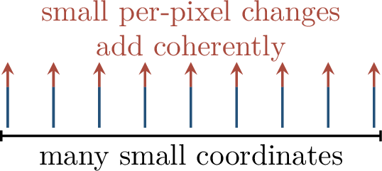
4.0.3 Robust Training and Tradeoffs↩︎
Definition 0.49 (Adversarial training). Given a model \(f_\theta\), loss \(\ell\), and perturbation set \(\Delta_\epsilon\), adversarial training solves \[\min_\theta \E_{(x,y)\sim\mathcal{D}} \left[ \max_{\delta\in\Delta_\epsilon} \ell(f_\theta(x+\delta),y) \right].\]
This objective is a min–max problem. The inner maximization searches for an attack and approximates the worst-case loss in a perturbation ball, while the outer minimization adjusts the model so that even the attacked examples are classified correctly. Projected gradient descent attacks and adversarial training are central in the modern empirical robustness literature [40].
In practice the inner maximization is often approximated by projected gradient descent. For \(\ell_\infty\)-bounded attacks, one initializes \(x_0=x+\eta_0\) and iterates \[x_{t+1} = \Pi_{B_\infty(x,\epsilon)} \left( x_t+\alpha\,\sign(\nabla_{x_t}\ell(f_\theta(x_t),y)) \right).\]
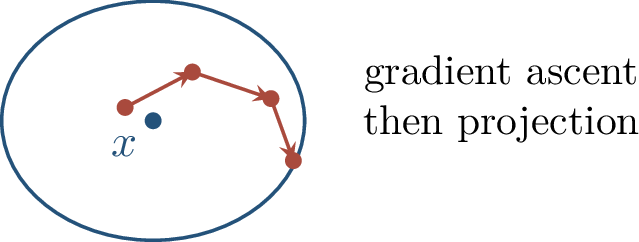
Definition 0.50 (Robustness certificate). A certificate proves that, for a given point \(x\), \[f(x+\delta)=f(x) \qquad \text{for all }\left\lVert \delta \right\rVert\le\epsilon.\] It is a rigorous lower bound on the local robust radius.
Empirical defenses try many attacks and report accuracy against them. Certified defenses use convex relaxations, randomized smoothing, interval bounds, or related methods to prove invariance in a ball. Empirical robustness can fail under a stronger attack; certificates are rigorous but often conservative.
Randomized smoothing is one important certification paradigm [41]. Instead of certifying the original classifier directly, one certifies a smoothed classifier obtained by averaging predictions under Gaussian noise. The price is that the certificate applies to the smoothed decision rule and typically gives conservative radii, but the benefit is a mathematically checkable guarantee.
Theorem 0.36 (Informal robustness–accuracy tradeoff). There are distributions where one classifier achieves high standard accuracy by using many weakly correlated features, while every adversarially robust classifier must ignore those features and accept lower standard accuracy.
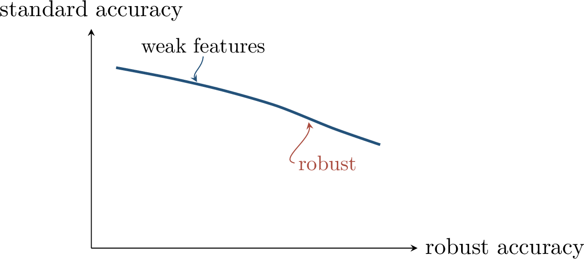
Example 0.8 (One robust feature and many fragile features). Let \(Y\in\{\pm1\}\). Suppose \[X_1=Y\quad\text{with high probability}, \qquad X_j\sim\mathcal{N}(\eta Y,1), \quad j=2,\ldots,d+1.\] The weak Gaussian features have small correlation \(\eta\) with \(Y\), but averaging many of them gives high standard accuracy by concentration. An \(\ell_\infty\) perturbation of size comparable to \(\eta\) can shift every weak coordinate in the wrong direction and erase this aggregate signal.
The lesson is not that weak features are useless. They may be precisely what gives excellent standard accuracy. The point is that robustness changes the set of acceptable features: a feature must remain predictive after the allowed perturbation, not merely on the original data distribution. This is why robust training can look statistically inefficient even when it improves worst-case behavior.
Robustness also includes attacks at training time. A test-time adversary perturbs \(x\) after the model is trained, while a training-time adversary can poison data or insert backdoor patterns before the learning algorithm sees the sample.
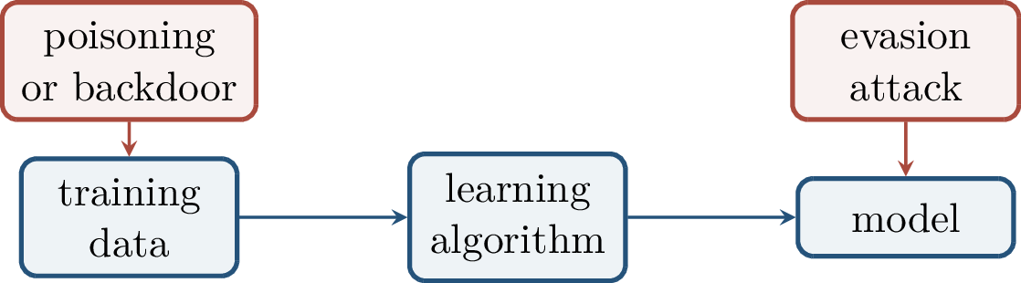
4.0.4 Generative Modeling↩︎
Generative modeling replaces prediction by distribution learning. Given samples \(x_1,\ldots,x_n\sim P_{\mathrm{data}}\), a generator \[G_\theta:\R^k\to\R^d, \qquad z\sim P_z, \qquad x=G_\theta(z),\] induces the pushforward distribution \(P_\theta=(G_\theta)_\#P_z\). The goal is to make \(P_\theta\) close to \(P_{\mathrm{data}}\).
This changes the object of learning. A discriminative model learns a map from \(x\) to \(y\); a generative model learns how probability mass is arranged in data space. The generator may be useful for sampling, density estimation, representation learning, compression, or downstream control. The theory depends heavily on which of these goals is being formalized.

The phrase “realistic sample” hides a mathematical choice: which distance or divergence between distributions should be optimized? Common choices include \[D_{\mathrm{KL}}(P_{\mathrm{data}}\Vert P_\theta), \qquad D_{\mathrm{JS}}(P_{\mathrm{data}},P_\theta), \qquad W_1(P_{\mathrm{data}},P_\theta),\] and integral probability metrics \[\sup_{f\in\mathcal{F}}\left|\E_P f-\E_Q f\right|.\] Likelihood rewards density estimation, adversarial distances reward indistinguishability by a discriminator class, and Wasserstein distance reflects geometry in data space.
No single divergence is universally best. Forward KL strongly penalizes placing low model density on real data, while adversarial objectives compare only through a chosen class of tests. Wasserstein distance is sensitive to how far mass must move, which is helpful when distributions have nearly disjoint low-dimensional supports. These choices lead to different optimization landscapes and different failure modes.

Definition 0.51 (Maximum likelihood). For a tractable density \(p_\theta(x)\), maximum likelihood solves \[\max_\theta \frac{1}{n}\sum_{i=1}^n \log p_\theta(x_i).\] At the population level this minimizes \(D_{\mathrm{KL}}(P_{\mathrm{data}}\Vert P_\theta)\).
The direction of the KL divergence matters. Maximum likelihood averages \(-\log p_\theta(x)\) over real data, so it severely penalizes missing regions where \(P_{\mathrm{data}}\) has mass. It does not directly penalize assigning extra probability to unrealistic regions unless that probability reduces the likelihood of real samples through normalization.
Autoregressive models make \[p_\theta(x)=\prod_j p_\theta(x_j\mid x_{<j})\] tractable. Normalizing flows use invertible maps and change of variables. Variational autoencoders optimize a lower bound when exact likelihood is hard.
Definition 0.52 (Implicit model). An implicit generator can sample from \(P_\theta\), but may not provide a tractable density \(p_\theta(x)\).
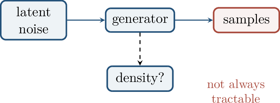
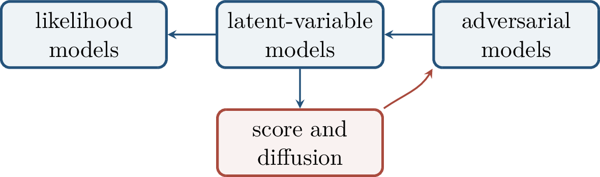
4.0.5 GAN Theory↩︎
Definition 0.53 (GAN minimax objective). Generative adversarial networks solve \[\min_G \max_D \left[ \E_{x\sim P_{\mathrm{data}}}\log D(x) + \E_{z\sim P_z}\log(1-D(G(z))) \right].\] The discriminator tries to distinguish real from generated samples, while the generator tries to fool it.
This is the original GAN formulation of Goodfellow et al. [18]. It is a population game in its clean mathematical form, but in practice it is solved with finite samples, finite networks, and alternating gradient steps. The gap between the population game and the trained system is one source of instability.
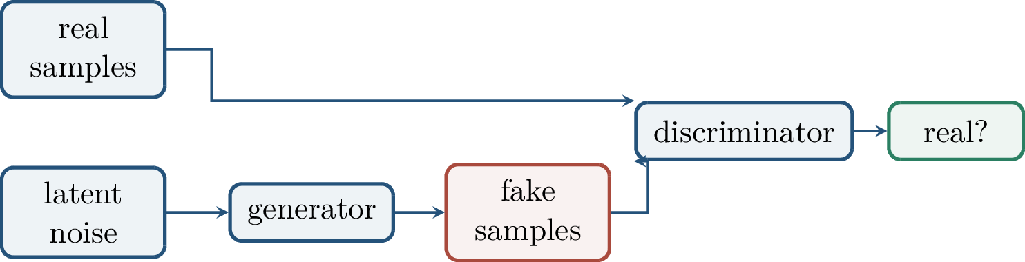
For a fixed generator distribution \(P_G\) with densities \(p_{\mathrm{data}}\) and \(p_G\), the optimal discriminator is \[D^*(x) = \frac{p_{\mathrm{data}}(x)}{p_{\mathrm{data}}(x)+p_G(x)}.\]
Proof. At each point \(x\), the discriminator maximizes an expression of the form \[a\log D+b\log(1-D),\] where \(a=p_{\mathrm{data}}(x)\) and \(b=p_G(x)\). Differentiating with respect to \(D\) gives \(a/D-b/(1-D)=0\), hence \(D=a/(a+b)\). ◻
Theorem 0.37 (Population GAN objective). With the optimal discriminator, \[V(D^*,G) = -\log4+2\,D_{\mathrm{JS}}(P_{\mathrm{data}}\Vert P_G).\] Therefore the global population optimum is achieved when \[P_G=P_{\mathrm{data}}.\]
The proof is a direct substitution of the optimal discriminator. Writing \(M=(P_{\mathrm{data}}+P_G)/2\), the value becomes \[-\log 4 + D_{\mathrm{KL}}(P_{\mathrm{data}}\Vert M) + D_{\mathrm{KL}}(P_G\Vert M),\] which is \(-\log4+2D_{\mathrm{JS}}(P_{\mathrm{data}}\Vert P_G)\) under the convention used here. Since Jensen–Shannon divergence is nonnegative and vanishes only when the two distributions agree, the population optimum is correct.
At infinite capacity and population level, the GAN objective targets the right distribution. In finite samples and finite networks, optimization and generalization become the hard parts. One reason is that the Jensen–Shannon divergence can produce poor local training signals when the supports of real and generated distributions do not overlap.
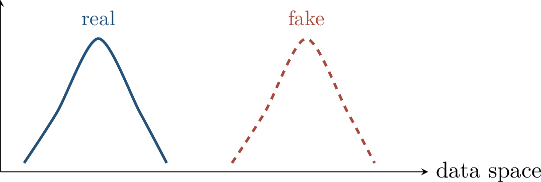
Definition 0.54 (Earth-mover distance). The 1-Wasserstein distance is \[W_1(P,Q) = \inf_{\pi\in\Pi(P,Q)} \E_{(X,Y)\sim\pi}\bigl[\left\lVert X-Y \right\rVert\bigr].\] It measures how much probability mass must move and how far.
The Kantorovich–Rubinstein duality writes \[W_1(P,Q) = \sup_{\operatorname{Lip}(f)\le1} \left(\E_P f-\E_Q f\right).\] In Wasserstein GANs, the discriminator is replaced by a 1-Lipschitz critic, which can provide smoother signals as supports move.
This is the motivation behind Wasserstein GANs [42]. The Lipschitz constraint is essential: without it, the critic could separate distributions by arbitrary jumps and the dual would no longer represent transport cost. In implementations, the constraint is enforced approximately, for example by weight clipping or gradient penalties [43].
Definition 0.55 (Mode collapse). Mode collapse occurs when a generator covers only a few modes of \(P_{\mathrm{data}}\) while still fooling a weak discriminator.
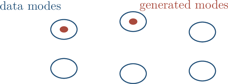
Generalization in GANs is naturally phrased through a discriminator class \(\mathcal{F}\), which defines the integral probability metric \[d_\mathcal{F}(P,Q) = \sup_{f\in\mathcal{F}} \left|\E_P f-\E_Q f\right|.\] Rich discriminators detect more differences but require more samples. Weak discriminators may miss mode collapse or memorization. This mirrors the role of test functions in SQ lower bounds: what the algorithm can distinguish depends on the class of statistics it is allowed to estimate.
This perspective also clarifies mode collapse. A generator can appear good against a weak discriminator because the missing modes are not detected by the available test functions. Strengthening the discriminator improves detectability, but it also increases optimization difficulty and sample complexity. Generative modeling is therefore not only about the generator architecture; it is also about the comparison principle used to judge it.
4.0.6 Deep Reinforcement Learning↩︎
Definition 0.56 (Markov decision process). An MDP is a tuple \[(\mathcal{S},\mathcal{A},P,r,\gamma),\] where \(s_t\in\mathcal{S}\), \(a_t\in\mathcal{A}\), \[s_{t+1}\sim P(\cdot\mid s_t,a_t),\] the reward is \(r(s_t,a_t)\), and \(\gamma\in(0,1)\) is a discount factor.
The Markov property says that the next-state distribution depends on the past only through the current state and action. This assumption is what makes dynamic programming possible. The discount factor \(\gamma\) makes the infinite-horizon return finite and gives future rewards less weight than immediate rewards; it will also make the Bellman operator a contraction.
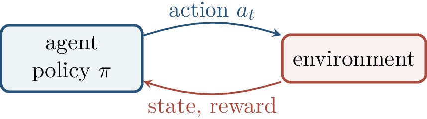
Definition 0.57 (Return, value, and Q-value). For a policy \(\pi\), \[J(\pi) = \E_\pi\left[\sum_{t=0}^{\infty}\gamma^t r(s_t,a_t)\right].\] The value and action-value functions are \[V^\pi(s) = \E_\pi\left[\sum_{t=0}^{\infty}\gamma^t r_t\mid s_0=s\right], \qquad Q^\pi(s,a) = \E_\pi\left[\sum_{t=0}^{\infty}\gamma^t r_t\mid s_0=s,a_0=a\right].\]
The value function is a compressed description of long-term consequence. It replaces the entire future trajectory distribution by one scalar expectation at each state. The \(Q\)-function is more directly useful for control because it compares actions at the same state; a greedy policy can choose an action with large \(Q(s,a)\).
For any policy \(\pi\), \[V^\pi(s) = \E_{a\sim\pi(\cdot\mid s)} \E_{s'\sim P(\cdot\mid s,a)} \left[r(s,a)+\gamma V^\pi(s')\right].\] The optimal value satisfies \[V^*(s) = \max_{a\in\mathcal{A}} \E_{s'\sim P(\cdot\mid s,a)} \left[r(s,a)+\gamma V^*(s')\right].\]
Theorem 0.38 (Bellman optimality operator). Define \[(TV)(s) = \max_a \E\!\left[r(s,a)+\gamma V(s')\mid s,a\right].\] Then \(T\) is a \(\gamma\)-contraction in the sup norm: \[\left\lVert TV-TU \right\rVert_\infty \le \gamma\left\lVert V-U \right\rVert_\infty.\]
Proof. The expectation is nonexpansive, the maximum over actions is nonexpansive in the sup norm, and the future value term is multiplied by \(\gamma\). ◻
The contraction theorem is the fundamental stability statement in tabular dynamic programming. It implies that value iteration converges to the unique fixed point \(V^*\). Deep reinforcement learning keeps this Bellman fixed point as a guiding equation, but replaces exact tables by function approximation, stochastic samples, and bootstrapped targets.
Deep Q-learning approximates \(Q^*(s,a)\) by a neural network \(Q_\theta(s,a)\). The target used in a temporal-difference update is \[y_t = r_t+\gamma\max_{a'}Q_{\theta^-}(s_{t+1},a'),\] and the squared loss is \[\left(Q_\theta(s_t,a_t)-y_t\right)^2.\] Experience replay reduces temporal correlation, while a target network \(\theta^-\) stabilizes the moving target.
The original deep Q-network work showed that these engineering choices can make neural value approximation work on high-dimensional visual inputs [44]. From a theory perspective, they address two sources of instability: the samples are not independent, and the target being regressed against depends on the same network being trained.
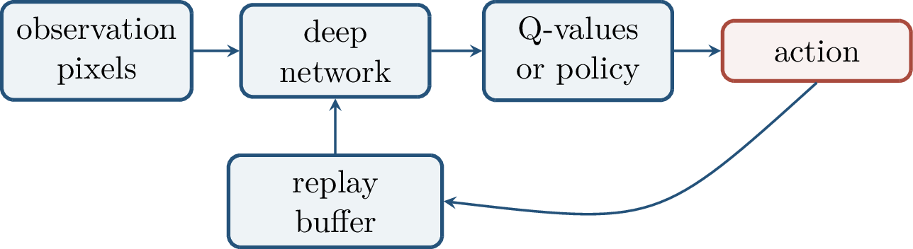
Deep RL is difficult both statistically and computationally. Data are dependent, exploration affects what is observed, rewards may be sparse or delayed, bootstrapping creates moving targets, and function approximation can amplify errors. In a single feedback loop it combines approximation, optimization, and control.
Classical reinforcement learning separates many of these issues in tabular or linear settings; see [45] for the standard framework. Deep RL combines them with high-dimensional representation learning. This is why results from supervised learning do not transfer mechanically: the learner is no longer observing a fixed distribution.
Theorem 0.39 (Policy-gradient identity). For a differentiable stochastic policy \(\pi_\theta\), \[\nabla_\theta J(\theta) = \E_{\tau\sim\pi_\theta} \left[ \sum_{t\ge0} \nabla_\theta\log\pi_\theta(a_t\mid s_t)\, G_t \right],\] where \(G_t\) is a return estimate from time \(t\).
The identity turns a derivative of an expectation over trajectories into an expectation of score-function terms. It can be estimated from sampled trajectories. Baselines reduce variance without changing the expectation.
The key algebra is the log-derivative trick: \[\nabla_\theta p_\theta(\tau) = p_\theta(\tau)\nabla_\theta\log p_\theta(\tau).\] For an MDP with policy \(\pi_\theta\), the transition probabilities do not depend on \(\theta\), so \[\nabla_\theta\log p_\theta(\tau) = \sum_t\nabla_\theta\log\pi_\theta(a_t\mid s_t).\] The resulting estimator is unbiased but can have high variance, which is why baselines, advantage functions, and actor–critic methods are central in practice.
4.0.7 Unifying View and Open Directions↩︎
The three themes share the same structural pattern. A classifier plays against an attacker, a generator plays against a discriminator, and a policy plays against an environment. In each case, the mathematics is about the stability of learning dynamics in a coupled system.
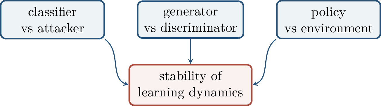
Several open questions remain central. Can robust training avoid losing useful nonrobust features? Which distributional metrics best predict human-perceived sample quality? When do adversarial games converge rather than cycle? Can deep RL be made sample efficient without brittle exploration heuristics? Which guarantees survive modern scale and pretraining? The next theory layer is not only about networks as function classes, but about networks embedded in games, simulators, and feedback loops.
Chapter Synthesis
Adversarial robustness replaces ordinary risk by a worst-case neighborhood requirement; dual norms explain first-order attacks and robust margins.
Adversarial training is a min–max procedure, while certificates aim to prove robustness rather than merely test it empirically.
Generative modeling learns distributions. Likelihood, adversarial games, and Wasserstein distance encode different notions of distributional closeness.
GAN theory is clean at the population level: the optimal discriminator converts the original objective into a Jensen–Shannon divergence. Finite capacity and optimization introduce the practical difficulties.
Reinforcement learning studies sequential decision making. Bellman equations provide fixed-point structure, while deep RL adds representation learning, bootstrapping, exploration, and feedback.
This chapter is based on the Chapter 10 Beamer source folder 408lec10_interlude_robust_generative_rl and the scanned reference note 408lec10post.pdf, whose main mathematical content is the interlude roadmap: adversarial
robustness, more generative models, and deep reinforcement learning. The added background uses the existing bibliography: adversarial examples and first-order attacks [17], [39], adversarial training [40], certified smoothing [41], GANs [18], Wasserstein GANs and gradient penalties [42], [43], deep Q-learning [44], and the standard
reinforcement-learning framework [45].
4.0.8 Motivation and Threat Models↩︎
The previous chapter introduced adversarial robustness as one of the first places where deep learning theory must look beyond the usual supervised learning pipeline. A classifier may achieve excellent standard test accuracy and still change its prediction under a perturbation that is small in a chosen metric. Chapter 11 develops this idea more systematically. It asks not only whether a trained model is stable at test time, but also whether the training procedure itself is stable when a small fraction of the data are corrupted.
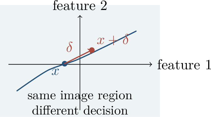
There are two principal locations where an adversary can act. A test-time adversary modifies the input after training. A training-time adversary modifies the data before the learner ever sees them. The first setting leads to evasion attacks and adversarial examples; the second leads to poisoning, backdoors, and robust statistics.
The distinction is useful because the mathematical object being protected is different. In evasion robustness, the trained classifier is fixed and the adversary searches locally around a test input. In poisoning robustness, the learning algorithm itself is attacked through its input sample. A defense against one threat model need not protect against the other: adversarial training may harden a classifier locally without detecting a backdoor in the training set, while robust statistics may remove outliers without certifying a local decision boundary.
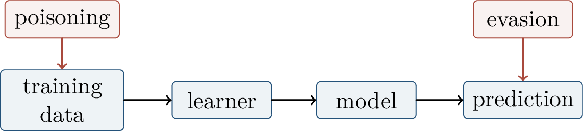
Definition 0.58 (Adversarial example). For a classifier \(f:\R^d\to[K]\), an input \(x\) with true label \(y\), a norm \(\left\lVert \cdot \right\rVert\), and a perturbation radius \(\epsilon>0\), an adversarial example is a point \[x'=x+\delta,\qquad \left\lVert \delta \right\rVert\le \epsilon,\qquad f(x')\ne y .\] In a targeted attack the adversary requires \(f(x')=t\) for a specified target label \(t\). In a black-box attack the adversary may not know the parameters of \(f\), but may exploit transfer from surrogate models or use queries to estimate a useful perturbation.
The norm ball is a threat model, not a complete theory of perceptual similarity. It is nevertheless valuable because it makes the adversary’s power explicit and reproducible. The modern empirical puzzle was that standard neural networks could be vulnerable to perturbations that are tiny in common norms [17]. The linearized calculation in the next section explains why this can happen even when each coordinate changes only slightly [39].
Definition 0.59 (Robust risk). Let \(\ell\) be a loss, let \(\mathcal{D}\) be the data distribution, and write \[\mathcal{B}_\epsilon(x)=\{x':\left\lVert x'-x \right\rVert\le \epsilon\}.\] The robust risk of \(f_\theta\) is \[R_{\mathrm{rob}}(\theta) = \E_{(x,y)\sim\mathcal{D}} \left[ \max_{x'\in \mathcal{B}_\epsilon(x)} \ell(f_\theta(x'),y) \right].\]
Standard empirical risk minimization asks the model to be correct at the observed points. Robust risk minimization asks it to be correct on a whole neighborhood around each point. That change turns learning into a local worst-case problem. It also makes the choice of norm and radius part of the modeling assumption: an \(\ell_\infty\) ball, an \(\ell_2\) ball, and a perceptual similarity set can encode very different notions of “small”.
Robust risk is also distribution dependent. The expectation is still over clean examples \((x,y)\sim\mathcal{D}\), but the loss is evaluated on a worst-case neighborhood of each clean input. Thus robust learning asks for a classifier whose predictions are stable around typical data, not necessarily throughout the entire ambient space.
4.0.9 Robust Optimization and Attacks↩︎
The central algorithmic idea in adversarial training is to approximate the robust risk by a finite-sample min–max objective. For a training set \(\{(x_i,y_i)\}_{i=1}^n\), Madry-style adversarial training solves \[\min_\theta \frac{1}{n}\sum_{i=1}^n \max_{\left\lVert \delta \right\rVert_p\le\epsilon} \ell\big(f_\theta(x_i+\delta),y_i\big).\] The inner problem searches for a hard nearby input; the outer problem fits parameters that survive those attacks.
This objective is the basis of projected-gradient adversarial training [40]. It should be read as an algorithmic approximation to robust risk, not as an exact solution of the inner maximization. In practice, the quality of adversarial training depends on the strength of the attack used during training, the number of random restarts, the perturbation geometry, and the capacity of the model.
Let \(L(x)\) be differentiable. The first-order approximation gives \[\max_{\left\lVert \delta \right\rVert_p\le\epsilon} L(x+\delta) \approx L(x)+ \max_{\left\lVert \delta \right\rVert_p\le\epsilon}\left\langle \nabla_x L(x),\delta \right\rangle = L(x)+\epsilon\left\lVert \nabla_x L(x) \right\rVert_q , \qquad \frac{1}{p}+\frac{1}{q}=1 .\] For \(p=\infty\), one maximizer is \[\delta_{\mathrm{FGSM}} = \epsilon\,\sign(\nabla_x L(x)).\]
Proof. The equality follows from Holder’s inequality and equality in the dual norm. For \(p=\infty\), the feasible set is a coordinatewise box. Each coordinate of \(\delta\) is chosen to have the sign of the corresponding coordinate of the gradient, which yields the fast gradient sign method. ◻
The fast gradient sign method is a one-step attack. Projected gradient descent (PGD) repeats a first-order step and projects back to the perturbation set: \[\delta_{t+1} = \Pi_{\left\lVert \delta \right\rVert\le\epsilon} \left( \delta_t+\alpha\,\sign(\nabla_\delta L(x+\delta_t)) \right).\] Several random starts are often used in practice, because a single failed attack is not evidence of robustness.
This warning is central. A model can appear robust because the attack optimization is poorly conditioned, because gradients are masked, or because the chosen attack is too weak. A certificate, introduced below, has a different status: it proves that no point in the specified perturbation set can change the prediction, regardless of whether a search algorithm finds one.
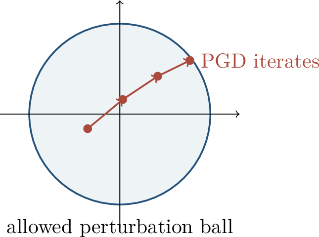
The geometry of robust classification can be understood as a margin condition. If an \(\epsilon\)-ball around a training point intersects a region classified with the wrong label, the point is not certified robust. A more flexible boundary may separate all perturbation balls, but this boundary can be more complex than the standard decision boundary and may be harder to learn.
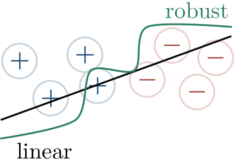
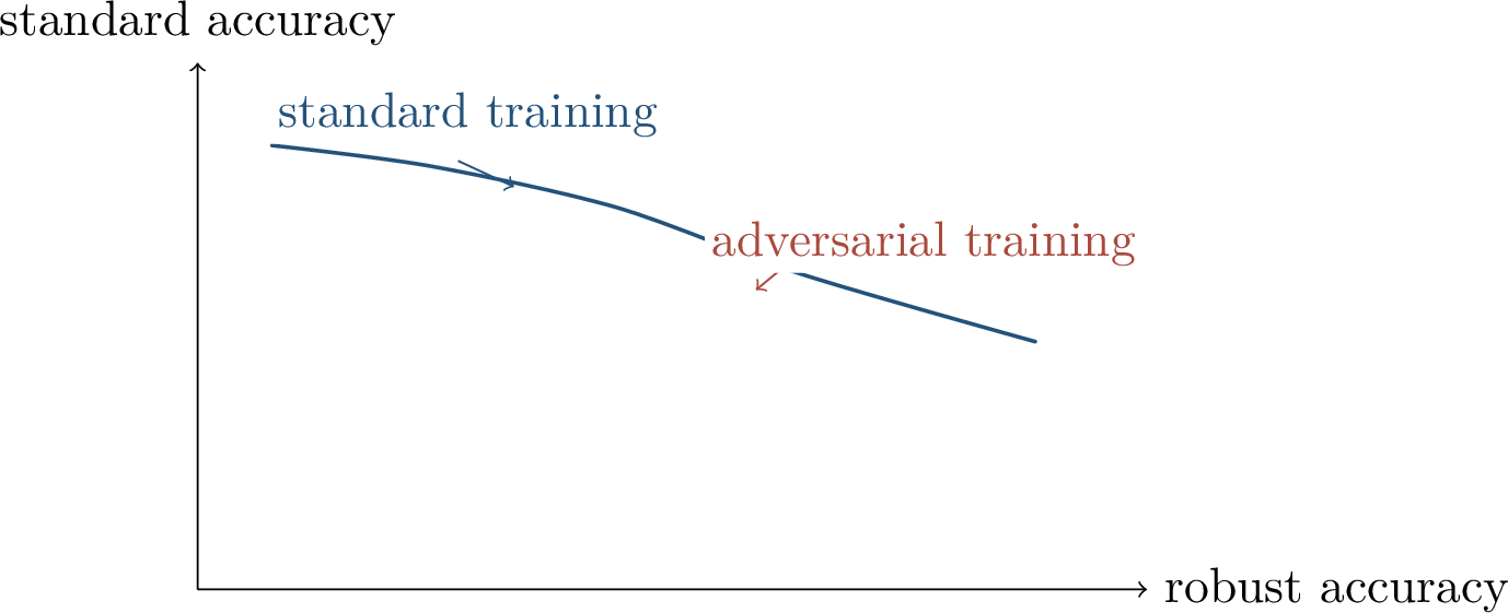
Definition 0.60 (Certified radius). For a fixed classifier \(f\), the local robust radius at \(x\) is \[r_f(x) = \inf_{\delta}\{\left\lVert \delta \right\rVert: f(x+\delta)\ne f(x)\}.\] A certification method proves a lower bound \(r_f(x)\ge r\), without relying on the success or failure of a particular attack algorithm.
This distinction matters. An attack is a search procedure; if it fails, the model may be robust, or the search may simply have missed a better perturbation. A certificate is a mathematical proof that no perturbation in a specified set changes the prediction.
The tradeoff is that certificates are often conservative. A loose certificate may fail to prove robustness even when the model is in fact robust. The design problem is therefore to find relaxations that are sound, computationally tractable, and tight enough to be useful at neural-network scale.
4.0.10 Certified Defenses↩︎
Suppose a neural network outputs logits \(z(x)\in\R^K\). For the true class \(y\), define the margin against class \(j\) by \[m_j(x)=z_y(x)-z_j(x).\]
If for every \(j\ne y\), \[\inf_{x'\in\mathcal{B}_\epsilon(x)} m_j(x')>0,\] then every point in \(\mathcal{B}_\epsilon(x)\) is classified as \(y\).
Proof. For every perturbed point \(x'\) and every wrong class \(j\ne y\), the condition says \(z_y(x')>z_j(x')\). Hence the largest logit is the \(y\)-logit throughout the perturbation ball. ◻
The challenge is that exact verification of ReLU networks is computationally hard. Certified defenses therefore replace the exact reachable set by a tractable outer approximation. Interval bounds, linear relaxations, and convex outer polytopes all follow this pattern: \[\{f(x+\delta):\left\lVert \delta \right\rVert\le\epsilon\} \subseteq \mathcal{P}_{\mathrm{relax}} .\] If the relaxed set still has positive margins, the original network is certified.
The word “outer” is essential. A relaxation used for certification may add fake activations that no true network input can realize, but it must never exclude a true activation. Soundness comes from containment; tightness comes from how little extra volume the relaxation introduces.
![Figure 203: For an ambiguous ReLU with preactivation interval [\ell,u], the convex hull gives a sound outer relaxation.](/article/2607.01311/ms-figure207.png "fig:")
Theorem 0.40 (Sound convex relaxation). For a ReLU network and an input perturbation polytope, replacing each ambiguous ReLU by its convex hull gives an outer polytope containing every possible activation vector. Consequently, if the relaxed optimization problem proves all wrong-class margins positive, the original nonlinear network is certified on the input perturbation set.
The proof is by induction over layers. At each layer the relaxed feasible set contains all exact activations that could have arisen from previous layers. A linear map preserves containment, and the convex ReLU hull contains the exact graph of the ReLU over the current interval. The final margin bound is sound because the exact outputs are a subset of the relaxed outputs.

Another simple certificate comes from Lipschitz continuity.
Suppose each margin \(m_j\) is \(L_j\)-Lipschitz with respect to \(\left\lVert \cdot \right\rVert\). If \[m_j(x)>L_j\epsilon \qquad \text{for all }j\ne y,\] then the classifier is robust on \(\mathcal{B}_\epsilon(x)\).
Proof. For \(\left\lVert x'-x \right\rVert\le\epsilon\), \[m_j(x')\ge m_j(x)-L_j\left\lVert x'-x \right\rVert>m_j(x)-L_j\epsilon>0 .\] Thus every wrong-class margin remains positive. ◻
Global Lipschitz constants are easy to state but often much too loose. Local and layerwise bounds can be sharper, but they require more careful analysis of the network around the point being certified.
This illustrates a common theme in certified robustness. The simplest bounds are usually global and compositional, so they multiply worst-case constants across layers. Stronger certificates use more local information about the input, activation pattern, or distribution of perturbations, but are typically more expensive to compute.
4.0.11 Randomized Smoothing via Privacy↩︎
Convex relaxations certify a deterministic network directly. Randomized defenses instead certify an averaged classifier. If \(h\) is a base classifier and \(\eta\) is random noise, one considers \[g(x)=\argmax_i \Prob(h(x+\eta)=i).\] The reference note explains a useful route to such certificates: first show that differentially private randomized scores are stable under input changes, then add noise to make the scores private with respect to the pixel metric.
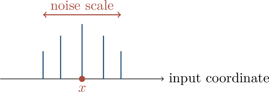
Definition 0.61 (Metric differential privacy). Let \(\rho\) be a metric on inputs. A randomized algorithm \(\mathcal{A}\) is \((\varepsilon,\delta)\)-private with respect to \(\rho\) if for all inputs \(x,x'\) and all measurable output events \(S\), \[\Prob(\mathcal{A}(x)\in S) \le e^{\varepsilon \rho(x,x')} \Prob(\mathcal{A}(x')\in S)+\delta .\] For adversarial robustness, the “database” is the image itself, and nearby databases are images that are close in a pixel norm.
This use of privacy is conceptual rather than sociological. A private mechanism cannot change its output distribution too much when its input is perturbed. If class scores are produced by such a mechanism and one class has a sufficiently large probability margin, then the predicted class is stable throughout the perturbation set.
Lemma 0.22 (Expectation stability). Suppose \(A(x)\in[0,b]\) is a randomized scalar output and is \((\varepsilon,\delta)\)-private for all pairs with \(\rho(x,x')\le1\). Then \[\E A(x) \le e^\varepsilon \E A(x')+b\delta .\]
Proof. Use the layer-cake identity \[\require{physics} \E A(x)=\int_0^b \Prob(A(x)>t)\,\dd t .\] For each threshold \(t\), apply the privacy inequality to the event \(\{A>t\}\). Integrating the resulting bound over \(t\in[0,b]\) gives \[\require{physics} \E A(x) \le e^\varepsilon\int_0^b\Prob(A(x')>t)\,\dd t + \int_0^b\delta\,\dd t = e^\varepsilon\E A(x')+b\delta .\] ◻
Let \(\mathcal{A}(x)\in[0,1]^K\) be a randomized score vector that is \((\varepsilon,\delta)\)-private for all \(\rho(x,x')\le1\), and define the deterministic classifier \[f(x)=\argmax_{k\in[K]}\E[\mathcal{A}_k(x)] .\] If for some label \(i\), \[\E[\mathcal{A}_i(x)] > e^{2\varepsilon}\max_{j\ne i}\E[\mathcal{A}_j(x)] +(1+e^\varepsilon)\delta ,\] then \(f(x')=i\) for every \(x'\) with \(\rho(x,x')\le1\).
Proof. Fix \(x'\) with \(\rho(x,x')\le1\). Applying the lemma in the reverse direction to coordinate \(i\) gives \[\E[\mathcal{A}_i(x')] \ge e^{-\varepsilon}\big(\E[\mathcal{A}_i(x)]-\delta\big).\] For any \(j\ne i\), applying the lemma in the forward direction gives \[\E[\mathcal{A}_j(x')] \le e^\varepsilon\E[\mathcal{A}_j(x)]+\delta .\] The assumed margin makes the lower bound for class \(i\) strictly larger than the upper bound for every other class, so the expected-score classifier remains label \(i\). ◻
How can a network produce private scores? One option is to add noise to an intermediate representation. Write the model as \[x \xrightarrow{g} h \xrightarrow{\mathrm{rest}} z .\] If we replace \(h=g(x)\) by \(\widetilde{h}=g(x)+\eta\), then the noise required for privacy depends on the sensitivity \[\Delta_{p,q}(g) = \sup_{x\ne x'} \frac{\left\lVert g(x)-g(x') \right\rVert_q}{\left\lVert x-x' \right\rVert_p}.\] For a first linear layer \(g(x)=Wx\), this is the operator norm \(\sup_{\left\lVert u \right\rVert_p=1}\left\lVert Wu \right\rVert_q\). Training or regularizing the network to make this sensitivity smaller allows less noise, and therefore less damage to accuracy.
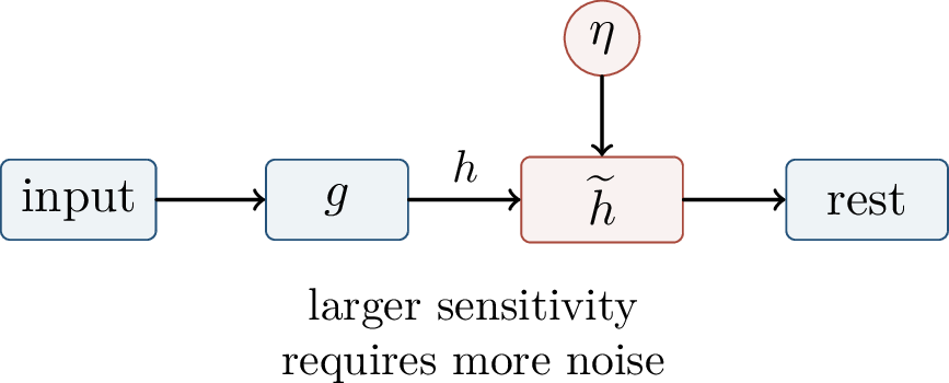
Definition 0.62 (Smoothed classifier). Given a base classifier \(h\) and Gaussian noise \(\eta\sim\mathcal{N}(0,\sigma^2 I)\), the smoothed classifier is \[g(x) = \argmax_{c\in[K]}\Prob\big(h(x+\eta)=c\big).\]
Theorem 0.41 (Gaussian smoothing certificate). Let \(p_A\) be a lower bound on the top class probability and \(p_B\) an upper bound on the runner-up probability. If \(p_A>p_B\), then the smoothed classifier is certifiably constant in an \(\ell_2\) ball of radius \[R = \frac{\sigma}{2} \left( \Phi^{-1}(p_A)-\Phi^{-1}(p_B) \right).\]
The proof uses the Neyman–Pearson structure of Gaussian shifts: if two inputs are close in \(\ell_2\), the two Gaussian neighborhoods overlap substantially, so a large enough top-class probability gap at \(x\) forces the same class to remain most likely at nearby \(x'\). Larger \(\sigma\) increases the possible radius, but too much noise can erase the signal used by the classifier.
Randomized smoothing is one of the cleanest certified defenses because it turns robustness into a probability comparison under Gaussian shifts [41]. The theorem is population-level: in experiments, one must estimate \(p_A\) and \(p_B\) from Monte Carlo samples and use statistical confidence bounds before reporting a certified radius.
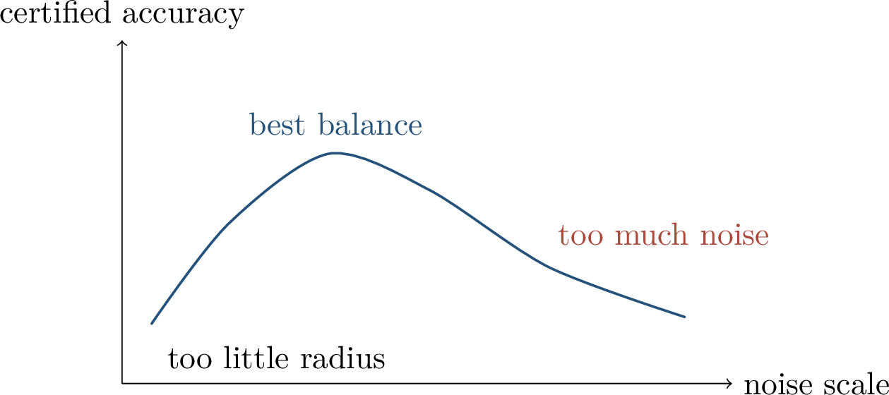
Gaussian smoothing naturally certifies \(\ell_2\) robustness, but it is not the only possible geometry. Other noise laws correspond to other norms and isoperimetric problems. The notes mention Wulff-crystal viewpoints, where the shape that minimizes boundary growth determines the best certificate geometry.
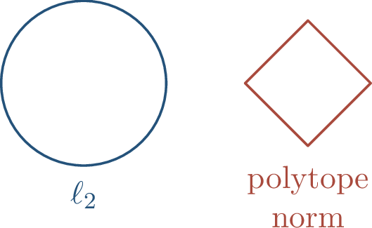
4.0.12 High-Dimensional Limits↩︎
The chapter next asks whether adversarial examples are an accident of current training methods or a geometric feature of high-dimensional spaces. Let \[E=\{x:\text{the classifier makes a mistake at }x\}\] be the error set, and define \[d(E)=\E_x[\operatorname{dist}(x,E)] .\] This quantity is the average Euclidean distance from a random point to the nearest error. Even if \(E\) has small measure, high-dimensional measure concentration can make \(E\) close to many points.
This is a useful abstraction because it separates the geometry of adversarial examples from the details of neural-network training. If small error sets expand rapidly in high dimension, then even a classifier with good standard accuracy may have many nearby errors. The question is then whether real data distributions have enough low-dimensional or semantic structure to escape this worst-case concentration picture.
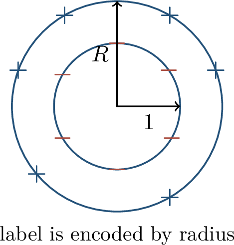
Theorem 0.42 (Spherical expansion). Let \(E\subseteq S^{d-1}\) be measurable with \(\mu(E)\ge 1/2\). If \[E_r=\{x\in S^{d-1}:\operatorname{dist}(x,E)\le r\},\] then \[\mu(E_r)\ge 1-2\exp(-c d r^2)\] for a universal constant \(c>0\).
The proof idea is the isoperimetric principle on the sphere: among all sets of fixed measure, spherical caps have the slowest neighborhood expansion. Hence if even a cap expands quickly, every other set of the same measure expands at least as quickly.
The theorem should be interpreted as a measure-concentration statement, not as a claim about a particular classifier architecture. It says that once the error set has nontrivial measure, its small Euclidean neighborhood can cover most of the sphere. This mechanism is one reason high-dimensional geometry keeps reappearing in robustness theory.
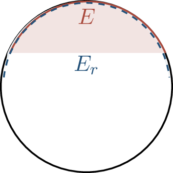
Theorem 0.43 (Informal adversarial sphere bound). For high-dimensional sphere data, any classifier with standard accuracy \(p>1/2\) has many points within distance \[O\!\left(\frac{\Phi^{-1}(p)}{\sqrt d}\right)\] of the error set.
The conclusion is a warning about geometry, not a proof that real-image robustness is impossible. Real images are not uniformly distributed on a sphere, human perception is not exactly an \(\ell_p\) norm, and data may lie near a structured low-dimensional manifold. The chapter note explicitly asks whether this explains practical adversarial examples and answers: likely not by itself.
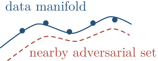
Theorem 0.44 (Informal robust learning separation). There are learning problems for which robust classifiers exist and are information-theoretically learnable, and for which nonrobust learning can be computationally efficient, but no statistical-query algorithm can efficiently find a robust classifier under the stated assumptions.
This separation clarifies that robustness may fail for several different reasons. It may be geometrically fragile, statistically sample inefficient, or computationally hard. The robust classifier may exist; the difficulty may be finding it with the algorithms available to us.
This is the same separation of roles that appeared earlier in the monograph: existence, information, computation, and optimization are distinct. A robust classifier may exist, and enough samples may identify it in principle, while a restricted algorithmic model such as statistical queries still cannot find it efficiently. Robustness therefore adds another layer to the usual approximation-generalization-optimization story.
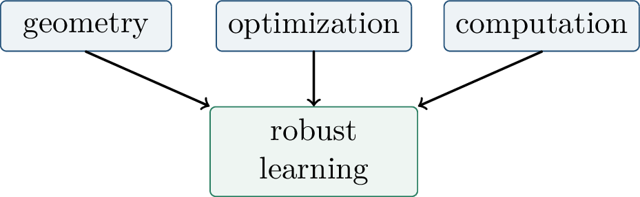
4.0.13 Poisoning and Robust Statistics↩︎
The second half of the chapter changes the location of the attack. Instead of perturbing a test input, the adversary corrupts the training sample. In the simplest abstraction, \[S_{\mathrm{obs}} = (1-\epsilon)S_{\mathrm{clean}} + \epsilon S_{\mathrm{bad}},\] where \(S_{\mathrm{bad}}\) is arbitrary. The goal may be to degrade global performance, or to implant a backdoor that activates only on inputs with a particular trigger.
Definition 0.63 (Huber contamination). The observed distribution is \[P_{\mathrm{obs}}=(1-\epsilon)P+\epsilon Q,\] where \(P\) is the target distribution and \(Q\) is arbitrary. The robust estimation problem is to estimate parameters of \(P\) from samples drawn from \(P_{\mathrm{obs}}\), with error proportional to the contamination level \(\epsilon\).
The model is pessimistic: \(Q\) can be chosen adversarially and need not have bounded moments, light tails, or any relation to \(P\). This is precisely why ordinary mean and covariance estimators are fragile. A single far-away point can dominate an average, so robust estimation must either reduce the influence of extreme points or identify directions in which the empirical distribution looks suspicious.
The one-dimensional Gaussian case already shows the core lesson. The empirical mean and variance can be made arbitrarily bad by moving a tiny corrupted mass far away. The median and the median absolute deviation do not react to a small number of extreme outliers in the same way.
Let the clean distribution be \(\mathcal{N}(\mu,\sigma^2)\), and suppose an \(\epsilon\)-fraction of the sample is corrupted. With enough samples, the empirical median \(\widehat\mu\) and \[\widehat\sigma = \frac{\operatorname{MAD}(X_1,\ldots,X_n)}{\Phi^{-1}(3/4)}\] estimate the clean Gaussian up to error proportional to \(\epsilon\). In total variation, the reference note records the folklore bound \[d_{\mathrm{TV}}\!\left( \mathcal{N}(\mu,\sigma^2), \mathcal{N}(\widehat\mu,\widehat\sigma^2) \right) \le 3\epsilon\] up to the usual finite-sample deviations.
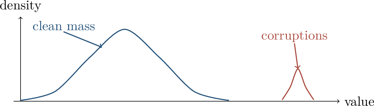
In high dimension, the situation is subtler. Corruptions can be placed in a direction where they move the empirical mean by order \(\epsilon\sqrt d\), and the adversarial direction may not be obvious until one projects the data.
The high-dimensional difficulty is not merely that there are many coordinates. It is that an adversary can hide corruption in a direction chosen after seeing the sample. Coordinatewise robust estimators miss such oblique directions, which is why modern algorithms inspect covariance structure and spectral deviations rather than treating coordinates independently.
Theorem 0.45 (Robust Gaussian estimation). Given \(\epsilon\)-corrupted samples from a high-dimensional Gaussian \(\mathcal{N}(\mu,\Sigma)\), there are polynomial-time algorithms that estimate \(\mu\) and \(\Sigma\) with total variation error \[d_{\mathrm{TV}}\big( \mathcal{N}(\mu,\Sigma), \mathcal{N}(\widehat\mu,\widehat\Sigma) \big) \le O\!\left(\epsilon\sqrt{\log(1/\epsilon)}\right)\] under standard sample-complexity assumptions.
The handwritten note also mentions related robust-estimation results with polylogarithmic factors, including bounds of the form \(O(\epsilon\log^{3/2}(1/\epsilon))\). The algorithmic theme is the same: search for directions in which the empirical moments are distorted, and filter points with suspiciously large influence in those directions.
This filtering paradigm mirrors the certification philosophy in the first half of the chapter. Instead of trusting an aggregate statistic, the algorithm looks for a certificate of failure: a direction whose empirical variance or mean shift is inconsistent with the clean model. If no such direction is found, the current estimate can be certified accurate under the model assumptions.
Definition 0.64 (Tukey depth). For a sample set \(S\subset\R^d\), the Tukey depth of \(x\) is \[\min_{\text{unit }v} \min\{ |\{y\in S:\left\langle v,y \right\rangle\le \left\langle v,x \right\rangle\}|, |\{y\in S:\left\langle v,y \right\rangle\ge \left\langle v,x \right\rangle\}| \}.\] The Tukey median is a point, not necessarily in \(S\), that maximizes Tukey depth.
The Tukey median is robust because it asks that \(x\) be central under every one-dimensional projection. The catch, emphasized in the reference note, is computational: exact Tukey median computation is hard in high dimension. The modern robust-statistics algorithms avoid this by using tractable spectral and filtering routines rather than enumerating all projections.
Tukey depth is nevertheless a useful idealization. It says what a robust center should mean geometrically: a good center cannot be separated from most of the data by any hyperplane. Spectral filtering can be viewed as a computationally tractable surrogate for this all-directions centrality condition.
Poisoning defenses for deep networks often use this spectral viewpoint after the network has learned a representation. For each predicted class, one collects hidden representations, centers them, and inspects the top singular direction. Points with unusually large projection onto that direction are candidates for poisoned or backdoored examples.
The spectral-signature method is most natural when a backdoor creates a feature direction shared by poisoned examples but not by clean examples of the same class [46]. The defense is therefore representation dependent: it works best after the network has organized clean examples into a relatively coherent class cluster and the poisoned examples introduce a detectable low-rank deviation.
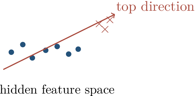
The statistical filtering step is only as good as the representation on which it operates. A backdoor may become visible as a feature-space cluster, but a sufficiently adaptive adversary can try to hide the cluster or attack the detector itself.
4.0.14 Influence, Interpretability, and Directions↩︎
The final topic is interpretability. Influence functions ask which training examples drive a prediction, rather than which input perturbation changes it.
Definition 0.65 (Influence of a training point). Let \(\widehat\theta\) minimize empirical risk and let \[H_{\widehat\theta} = \nabla_\theta^2 \frac{1}{n}\sum_i \ell(z_i,\widehat\theta).\] The first-order effect of upweighting a training point \(z\) on a test loss is \[I(z,z_{\mathrm{test}}) = - \nabla_\theta \ell(z_{\mathrm{test}},\widehat\theta)^\top H_{\widehat\theta}^{-1} \nabla_\theta \ell(z,\widehat\theta).\]
This formula is the deep-learning version of the influence curve from robust statistics: it approximates the change in an estimator when a single point is upweighted. In neural networks the approximation can be limited by nonconvexity and Hessian conditioning, but it still gives a useful diagnostic. If a test point is misclassified, influence functions can identify training examples that may explain the error; they can also reveal whether a prediction is driven by meaningful semantic similarity or by accidental correlations such as background or lighting.
Influence functions connect robustness with interpretability [47]. They do not certify robustness, and their linearization can fail when retraining would move parameters far from \(\widehat\theta\). Still, they provide a principled first-order way to ask which training examples support or undermine a prediction.
| Threat | Mathematical object | Typical defense |
|---|---|---|
| Evasion | local input ball | adversarial training, certificates |
| Random noise | smoothed decision rule | probability-gap certification |
| Geometry limit | expansion of the error set | representation and metric design |
| Poisoning | contaminated samples | robust statistics, filtering |
| Backdoors | hidden feature cluster | spectral signatures |
The limitations are important. Norm balls are convenient but imperfect proxies for human perception. Certificates can be conservative or expensive at scale. Robust accuracy may conflict with standard accuracy. Poisoning defenses depend on assumptions about the clean feature structure. Adaptive adversaries can target the defense itself.
The chapter closes with a broad challenge: find robustness notions that are simultaneously semantic, certifiable, learnable, and computationally tractable. This challenge ties together approximation, optimization, statistics, geometry, and computation, which is why robustness remains a central topic in deep learning theory.
Chapter Synthesis
Evasion and poisoning are different threat models: the former attacks test inputs, while the latter corrupts the training sample or representation.
First-order adversarial attacks arise from dual norms. PGD strengthens FGSM by repeatedly maximizing the loss inside the perturbation set.
Certified defenses prove robustness by bounding all possible perturbations, using margins, convex relaxations, Lipschitz bounds, or randomized smoothing.
High-dimensional geometry can make small error sets close to many points, but real data geometry and semantic metrics complicate the picture.
Poisoning defenses draw on robust statistics: contamination models, filtering, Tukey depth, spectral signatures, and influence functions all ask which points or directions have too much leverage.
This chapter is based on the Chapter 11 Beamer source folder, its seven section files on adversarial robustness and poisoning, and the handwritten reference note for Chapter 11. Key references named in the slides include Szegedy et al. on adversarial examples [17]; Goodfellow, Shlens, and Szegedy on FGSM [39]; Madry et al. on adversarial training [40]; Cohen, Rosenfeld, and Kolter on randomized smoothing [41]; Tran, Li, and Madry on spectral signatures [46]; and Koh and Liang on influence functions [47]. The monograph also discuss convex outer adversarial polytopes, privacy certificates, non-Gaussian smoothing shapes, adversarial spheres, computational constraints, and high-dimensional robust estimation.
4.0.15 Generative Modeling as Distribution Matching↩︎
The previous chapters studied learning mostly through supervised risk, optimization, stability, and adversarial robustness. This chapter shifts the object of learning. A generative model is not asked merely to predict a label from an input; it is asked to produce new samples whose law resembles the law that produced the training data. The central mathematical question is therefore a question about probability distributions.
This change of object also changes the meaning of success. In supervised learning the learner is evaluated on pairs \((x,y)\), and the risk is usually defined through a pointwise loss. In generative modeling there may be no canonical target output for a given latent seed. A generated image is good not because it matches one particular training image, but because the ensemble of generated images has the right distributional behavior. This is why the chapter begins with distribution matching rather than with a standard regression or classification loss.
Let \(P_{\mathrm{data}}\) denote the unknown distribution of real examples on \(\R^d\). A deep generator takes a simple random seed \(Z\sim P_Z\), usually a Gaussian or uniform distribution in a lower-dimensional latent space, and maps it to a synthetic sample \[\widetilde{X} = G_\theta(Z).\] The model distribution is the push-forward \[P_\theta = (G_\theta)_\# P_Z ,\] meaning that \(P_\theta(A)=P_Z(G_\theta^{-1}(A))\) for every measurable set \(A\). Thus the network architecture, the latent distribution, and the parameters \(\theta\) together define a family of probability laws.
Equivalently, for every bounded measurable test function \(f\), \[\E_{\widetilde{X}\sim P_\theta} f(\widetilde{X}) = \E_{Z\sim P_Z} f(G_\theta(Z)).\] This identity is often the most convenient way to reason about generators, because training objectives are written as expectations over samples. Notice also the geometric consequence of the push-forward construction. If the latent dimension \(k\) is much smaller than the ambient dimension \(d\), then the range of a regular generator is a low-dimensional subset of \(\R^d\). Hence \(P_\theta\) may be singular with respect to Lebesgue measure even though it produces visually rich samples. This observation will be important when we compare Jensen-Shannon and Wasserstein objectives.
This viewpoint is useful because it separates two tasks that are often blurred in practice. First, one must choose a discrepancy that says when two probability laws look close. Second, one must optimize the generator parameters so that the induced law is close to the data law under that discrepancy. Different generative-model families differ in the way they answer these two questions.
Definition 0.66 (Test-function distance). Let \(\mathcal{F}\) be a class of real-valued measurable functions. The integral probability metric generated by \(\mathcal{F}\) is \[d_\mathcal{F}(P,Q) = \sup_{f\in\mathcal{F}} \left| \E_{X\sim P}f(X)-\E_{Y\sim Q}f(Y) \right|.\] A model \(Q\) is realistic relative to \(\mathcal{F}\) if no test in \(\mathcal{F}\) can reliably separate expectations under \(P_{\mathrm{data}}\) and \(Q\).
The class \(\mathcal{F}\) specifies the resolution of the comparison. If \(\mathcal{F}\) contains all bounded measurable tests, then the distance becomes essentially a total-variation comparison, which is extremely sensitive to support mismatch. If \(\mathcal{F}\) is the unit ball of Lipschitz functions, then the same template leads to the dual form of the Wasserstein-1 distance under the usual moment assumptions. If \(\mathcal{F}\) is a neural-network class, then the distance asks only whether neural discriminators of that size can tell the two laws apart. These three choices can give very different answers for the same pair of distributions.
Generative adversarial networks (GANs) instantiate this idea by making the tests neural networks. The discriminator or critic is not merely an auxiliary optimization device; it also defines the statistical resolution at which real and generated distributions are compared. A small discriminator class may miss some discrepancies but can generalize from fewer samples. A large class can detect more discrepancies but may be statistically and computationally harder to control.
This perspective is deliberately modest. It does not say that fooling a chosen discriminator class is the same as matching the true data distribution in every possible sense. Rather, it gives a mathematically tractable proxy: the generator should remove all discrepancies that are visible to the tests we can train and analyze. Much of GAN theory is an attempt to understand when this proxy is statistically meaningful and when it is merely an artifact of a weak discriminator.
Deep learning enters at two places. The generator represents a complicated low-dimensional image of latent space in the ambient data space. The discriminator represents a learned statistical test. Alternating training creates a game between these two networks, and the same generator can later serve as a prior in inverse problems such as inpainting.
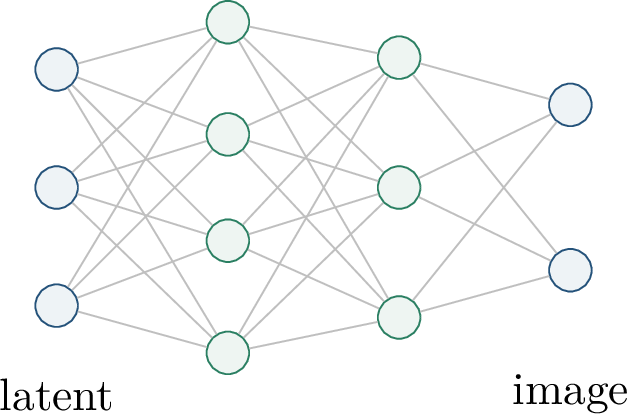
This chapter follows three questions. What divergence is optimized by the ideal GAN objective? What does finite data allow us to prove when classical distances are too strong in high dimension? Why can a generator, once learned, replace handcrafted priors in inverse problems?
4.0.16 The Ideal GAN Objective↩︎
The original GAN formulation is an adversarial game between a generator and a binary discriminator. The generator transforms latent noise into synthetic data. The discriminator receives either a real sample or a generated sample and tries to output a large value for real data and a small value for generated data. The formulation below is the population version of the original GAN objective of Goodfellow et al. [18]. Empirical training replaces the expectations by minibatch averages and restricts both players to parameterized neural networks.
Definition 0.67 (GAN game). Let \(X\sim P\), let \(Z\sim P_Z\), and let \(Q_\theta=(G_\theta)_\#P_Z\). For a discriminator \(D_\psi:\R^d\to[0,1]\), the population GAN objective is \[\begin{align} \min_\theta\max_\psi\;V(\theta,\psi), \qquad V(\theta,\psi) &= \E_{X\sim P}\log D_\psi(X)\\ &\quad+ \E_{Z\sim P_Z}\log\!\bigl(1-D_\psi(G_\theta(Z))\bigr). \end{align}\]
The signs in this objective are worth reading carefully. For fixed \(\theta\), the discriminator maximizes a binary log-likelihood: real samples should receive probability close to one, and generated samples should receive probability close to zero. For fixed discriminator parameters, the generator minimizes the same value by changing \(Q_\theta\) so that generated samples look real to \(D_\psi\). Thus the loss is not a single-player empirical risk but a coupled saddle objective. Even before optimization difficulties appear, one must understand what distributional discrepancy this saddle objective is trying to minimize.
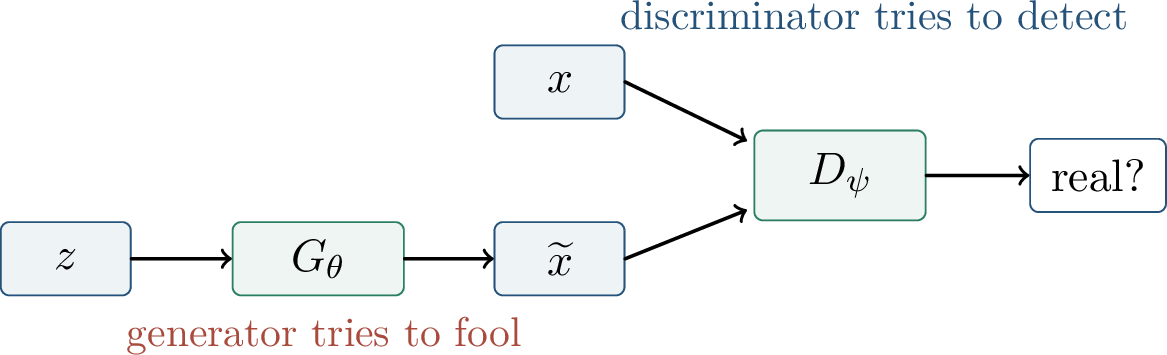
To understand the population objective, first freeze the generator and optimize over all possible discriminators. This idealization ignores the finite neural architecture but reveals the divergence hidden inside the loss.
Lemma 0.23 (Pointwise optimal discriminator). Assume \(P\) and \(Q\) have densities \(p\) and \(q\) with respect to a common measure. If discriminators range over all measurable functions \(\R^d\to[0,1]\), then the maximizer of \[\E_{X\sim P}\log D(X)+\E_{Y\sim Q}\log(1-D(Y))\] is \[D^*(x)=\frac{p(x)}{p(x)+q(x)} \qquad\text{whenever }p(x)+q(x)>0 .\]
Proof. For a fixed generator distribution \(Q\), the discriminator objective can be written as \[\require{physics} \begin{align} V(D,Q) &= \int p(x)\log D(x)\,\dd x + \int q(x)\log(1-D(x))\,\dd x\\ &= \int \bigl[p(x)\log D(x)+q(x)\log(1-D(x))\bigr]\,\dd x . \end{align}\] Thus the maximization separates pointwise in \(x\). For fixed nonnegative numbers \(p,q\), maximize \(p\log d+q\log(1-d)\) over \(0\le d\le1\). At an interior maximizer, \[\frac{p}{d}-\frac{q}{1-d}=0, \qquad\text{hence}\qquad d=\frac{p}{p+q}.\] The boundary cases are consistent with the same formula when one of \(p,q\) is zero. If the supports are disjoint, this discriminator perfectly identifies which distribution produced the sample on the union of the two supports. ◻
The formula also has a statistical interpretation. If a sample is drawn from the mixture that first flips a fair coin and then draws from \(P\) or \(Q\), then \(D^*(x)\) is the posterior probability that the coin selected the real distribution. The optimal discriminator is therefore the Bayes classifier for the two-sample hypothesis test.
Example 0.9 (Two extreme discriminator regimes). If \(P=Q\), then \(p=q\) and the optimal discriminator is \(D^*(x)=1/2\) almost everywhere. No observation carries information about which source generated the sample. At the other extreme, if \(P\) and \(Q\) are supported on disjoint measurable sets, then \(D^*\) can be chosen to equal one on the support of \(P\) and zero on the support of \(Q\). In this case the classification problem is trivial even if the two supports are geometrically very close. This second case is the reason support geometry matters for GAN training.
Definition 0.68 (KL and Jensen-Shannon divergences). For distributions \(P,Q\) with densities \(p,q\), the Kullback-Leibler divergence is \[\require{physics} \KL(P\Vert Q)=\int p(x)\log\frac{p(x)}{q(x)}\,\dd x ,\] with the usual convention that the value is \(+\infty\) if \(P\) is not absolutely continuous with respect to \(Q\). For \(M=\frac{1}{2}(P+Q)\), the Jensen-Shannon divergence is \[D_{\mathrm{JS}}(P\Vert Q) = \frac{1}{2}\KL(P\Vert M) + \frac{1}{2}\KL(Q\Vert M).\]
Gibbs’ inequality gives \(\KL(P\Vert Q)\ge0\), with equality only when \(P=Q\) almost surely. The Jensen-Shannon divergence inherits nonnegativity and is always finite when \(P\) and \(Q\) are probability measures. It equals \(\log 2\) when the two distributions are mutually singular.
Theorem 0.46 (Ideal GAN objective). With an unrestricted discriminator class, \[\max_D V(D,Q) = -\log 4 + 2\,D_{\mathrm{JS}}(P\Vert Q).\] Consequently, if the generator family can represent \(P\), the population optimum is attained exactly at \(Q=P\).
Proof. Substituting \(D^*(x)=p(x)/(p(x)+q(x))\) gives \[\require{physics} \begin{align} \max_D V(D,Q) &= \int p(x)\log\frac{p(x)}{p(x)+q(x)}\,\dd x + \int q(x)\log\frac{q(x)}{p(x)+q(x)}\,\dd x\\ &= \int p(x)\log\frac{p(x)}{2m(x)}\,\dd x + \int q(x)\log\frac{q(x)}{2m(x)}\,\dd x , \end{align}\] where \(m=(p+q)/2\). Pulling out the two factors of \(\log 2\) yields \[\max_D V(D,Q) = -2\log2+\KL(P\Vert M)+\KL(Q\Vert M) = -\log4+2\,D_{\mathrm{JS}}(P\Vert Q).\] The last statement follows from nonnegativity of \(D_{\mathrm{JS}}\), with equality iff \(P=Q\). ◻
This theorem is the clean population story behind the original GAN objective: an ideal discriminator turns the adversarial game into Jensen-Shannon minimization. It is also the first warning. A theorem about the population value of an idealized objective is not a theorem that practical alternating training is stable, nor that the discriminator gradients are useful everywhere.
Another practical distinction is sometimes hidden by the minimax notation. The generator update used in implementations is often the “non-saturating” variant, which maximizes \(\E_Z\log D_\psi(G_\theta(Z))\) rather than directly minimizing \(\E_Z\log(1-D_\psi(G_\theta(Z)))\). This change gives stronger gradients when the discriminator is confident, but it does not change the population calculation above: the ideal value of the original minimax game is still governed by Jensen-Shannon divergence.
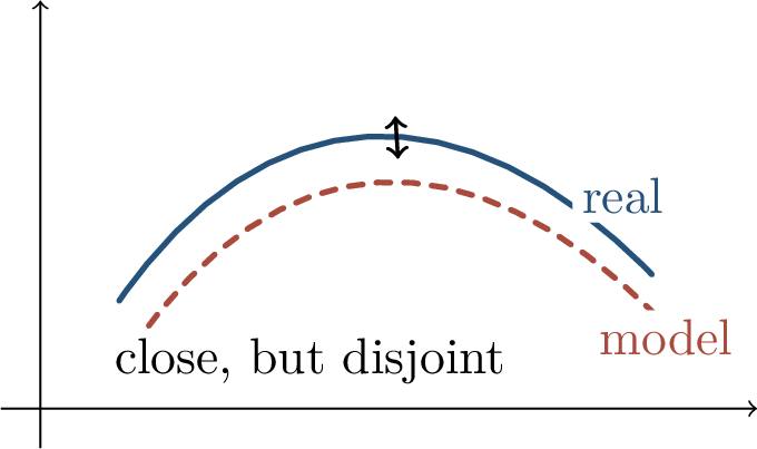
The geometric issue is especially visible in high dimension. Data may concentrate near a thin manifold, while the generator range is another thin manifold. If the two supports are disjoint, the optimal discriminator can separate them perfectly and \(D_{\mathrm{JS}}(P\Vert Q)=\log2\). The value no longer tells the generator how far it is from the data manifold. This motivates replacing classification by a geometry-sensitive discrepancy.
The point is not that Jensen-Shannon divergence is mathematically defective. It is a perfectly valid divergence between probability laws. The issue is compatibility with the geometry induced by low-dimensional generative models. When small movements of the generator range leave the supports disjoint, a classification divergence may remain flat exactly in the region where the generator needs directional information.
4.0.17 Wasserstein GANs↩︎
The Wasserstein viewpoint compares distributions by the cost of transporting mass. Instead of asking whether the supports overlap, it asks how far mass must be moved to transform one law into the other. This is the key motivation behind Wasserstein GANs [42]: when the generated manifold is close to the data manifold but not overlapping it, a transport distance can still provide a meaningful gradient-like signal.
Definition 0.69 (Wasserstein-1 distance). For probability distributions \(P,Q\) on a metric space, \[W_1(P,Q) = \inf_{\gamma\in\Pi(P,Q)} \E_{(X,Y)\sim\gamma}\left\lVert X-Y \right\rVert,\] where \(\Pi(P,Q)\) is the set of all couplings with marginals \(P\) and \(Q\).
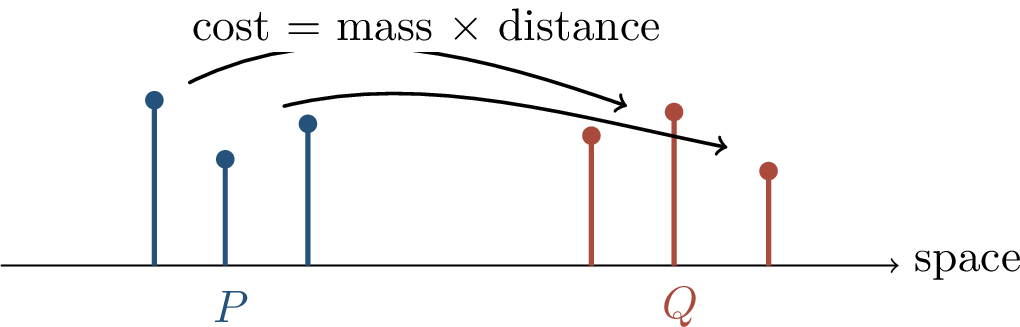
For generative modeling, the most important form of \(W_1\) is its dual representation.
Theorem 0.47 (Kantorovich-Rubinstein duality). On a Polish metric space with finite first moments, \[W_1(P,Q) = \sup_{\left\lVert f \right\rVert_{\operatorname{Lip}}\le1} \left[ \E_{X\sim P}f(X)-\E_{Y\sim Q}f(Y) \right].\] The supremum is over all 1-Lipschitz real-valued functions.
The dual turns the discriminator into a critic. A classifier outputs a probability of being real; a critic outputs a real score. The Lipschitz constraint prevents arbitrarily sharp spikes and makes the objective measure transport geometry.
The theorem also explains why the critic is allowed to output arbitrary real numbers. Its role is not to estimate a posterior probability, but to define a potential whose expectation gap measures how much mass must move. The Lipschitz constraint is the price paid for this geometric interpretation. If it were removed, the critic could amplify tiny support differences without bound and the objective would no longer represent \(W_1\).
Definition 0.70 (Wasserstein GAN objective). The ideal Wasserstein GAN solves \[\min_\theta \max_{\left\lVert f_\psi \right\rVert_{\operatorname{Lip}}\le1} \E_{X\sim P}f_\psi(X) - \E_{Z\sim P_Z}f_\psi(G_\theta(Z)).\] If the critic class contains all 1-Lipschitz functions and the generator can represent \(Q\), optimizing this objective minimizes \(W_1(P,Q)\).
The gain can be seen on the simplest possible example. Let \(P=\delta_0\) and \(Q_t=\delta_t\) on \(\R\). Then \[D_{\mathrm{JS}}(P\Vert Q_t)=\log2\quad(t\ne0), \qquad W_1(P,Q_t)=|t|.\] The Jensen-Shannon divergence is flat as soon as the point masses differ; the Wasserstein distance changes continuously with the shift.
This toy example captures the intended behavior of WGANs in a form that can be computed by hand. For \(t>0\), the only coupling between \(\delta_0\) and \(\delta_t\) transports unit mass from \(0\) to \(t\), so the transport cost is \(|t|\). A valid 1-Lipschitz critic achieving the dual value is \(f(x)=-x\) when \(t>0\), since \(\E_{\delta_0}f-\E_{\delta_t}f=t\). By contrast, the two point masses are mutually singular for every nonzero \(t\), so the Jensen-Shannon value does not distinguish a tiny displacement from a large one.
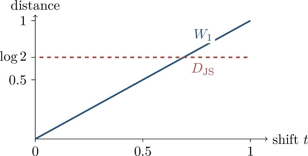
In practice, enforcing the exact Lipschitz constraint is difficult. The original WGAN used weight clipping. Later variants introduced gradient penalties, encouraging \[\left\lVert \nabla_x f_\psi(x) \right\rVert_2\approx1\] on interpolated samples, and spectral normalization, which constrains layer operator norms. These are useful optimization heuristics, but they are not identical to optimizing over the full unit Lipschitz ball. The gradient penalty approach of Gulrajani et al. [43], for example, enforces a local condition on samples drawn from a chosen interpolation distribution. It often stabilizes training, but the theoretical duality above concerns a global Lipschitz constraint over the entire space.
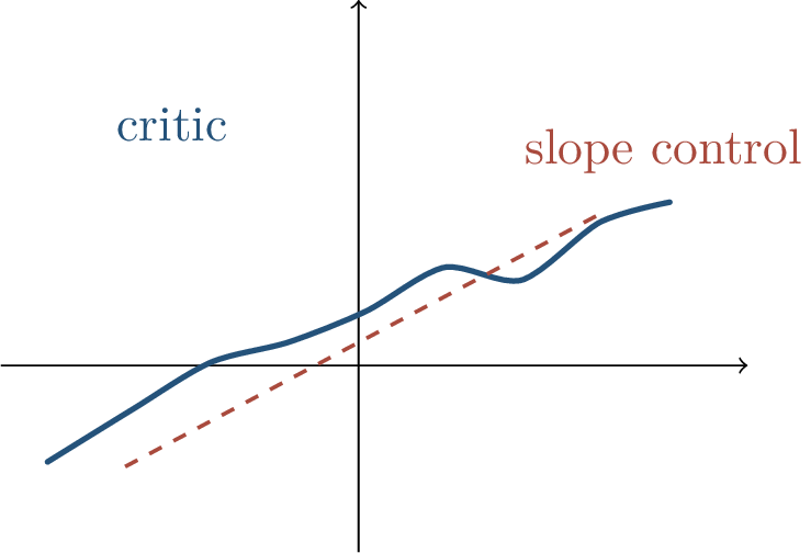
Replacing Jensen-Shannon divergence by \(W_1\) addresses one important geometric pathology: disjoint supports no longer force a saturated objective. It does not make the GAN problem convex, remove mode collapse, or guarantee that a neural critic has found the exact Kantorovich potential. The WGAN objective should therefore be read as a better-aligned discrepancy, not as a complete solution to adversarial training.
4.0.18 Finite Samples and Neural Distances↩︎
The preceding discussion used population distributions. Real training uses samples. This creates a subtle problem: in high dimensions the empirical distribution can be far from the population distribution under strong distances, even when the training sample is perfectly representative for learning purposes. Thus a satisfactory theory of GAN generalization cannot simply say that the empirical measure is close to the data distribution under a classical strong metric. It must say that the empirical and population objectives are close for the discriminators used by the algorithm.
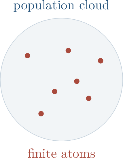
Let \(P=\mathcal{N}(0,I_d/d)\), and let \(\widehat P_m\) be the empirical distribution from \(m=\operatorname{poly}(d)\) independent samples. With high probability, \[D_{\mathrm{JS}}(P\Vert \widehat P_m)=\log2, \qquad W_1(P,\widehat P_m)\not\approx0 .\]
The first statement follows from mutual singularity: \(P\) is continuous while \(\widehat P_m\) is supported on finitely many atoms. The second reflects the curse of dimensionality in empirical optimal transport. The lesson is not that the sample is useless. The lesson is that the chosen distance is asking for too much.
This proposition should be interpreted as a warning about metrics rather than as a pessimistic statement about learning. A polynomial number of samples from a Gaussian may estimate many low-complexity expectations accurately, even though it cannot make the empirical distribution close in total variation or Wasserstein distance at a dimension-free rate. Restricted neural distances formalize exactly this weaker and more useful notion of closeness.
Arora, Ge, Liang, Ma, and Zhang propose measuring distributions only through the discriminators we actually intend to use.
Definition 0.71 (Restricted discriminator distance). Let \(\mathcal{F}\) be a class of discriminators \(D:\R^d\to[0,1]\), and let \(\phi\) be concave. Define \[\begin{align} d_{\mathcal{F},\phi}(P,Q) &= \sup_{D\in\mathcal{F}} \Bigl[ \E_{X\sim P}\phi(D(X)) + \E_{Y\sim Q}\phi(1-D(Y)) -2\phi(1/2) \Bigr]. \end{align}\]
This is a finite-resolution version of indistinguishability. If \(d_{\mathcal{F},\phi}(P,Q)\) is small, then no discriminator in \(\mathcal{F}\) can extract much more payoff from the real/generated distinction than it obtains from random guessing. When \(\mathcal{F}\) is a neural-network class with controlled complexity, this distance can generalize from a number of samples that scales with the number of discriminator parameters rather than with the ambient dimension in a classical nonparametric way.
The subtraction of \(2\phi(1/2)\) simply normalizes the distance so that a discriminator forced to guess \(D(x)=1/2\) gives value zero. The concavity of \(\phi\) is compatible with the binary-classification losses used in GANs, and the Lipschitz assumption on \(\phi\) lets one transfer approximation errors in the discriminator output into errors in the payoff. These technical conditions are not decoration; they are what allow covering-number and concentration arguments to control the supremum over \(\mathcal{F}\).
Theorem 0.48 (Uniform convergence for neural discriminator distances). Suppose \(\phi\) is concave, bounded in \([-\Delta,\Delta]\), and \(L_\phi\)-Lipschitz. Suppose the discriminator class has \(n\) parameters and is \(L\)-Lipschitz in those parameters. If \[m \gtrsim \frac{n\Delta^2\log(L_\phi L n/\varepsilon)}{\varepsilon^2},\] then with high probability, \[\left| d_{\mathcal{F},\phi}(\widehat P,\widehat Q) - d_{\mathcal{F},\phi}(P,Q) \right| \le \varepsilon .\]
Proof idea. Cover the discriminator parameter space by a finite \(\varepsilon\)-net. For a fixed net point, the empirical discriminator payoff concentrates by a standard bounded-difference or Hoeffding argument. A union bound controls all net points simultaneously. Finally, Lipschitz dependence on parameters transfers the control from the net to every discriminator in the original class. The logarithm of the covering number is proportional to the parameter count \(n\), which explains the form of the sample complexity. ◻
More explicitly, for each discriminator \(D\) define the payoff \[H_D(P,Q) = \E_{X\sim P}\phi(D(X)) + \E_{Y\sim Q}\phi(1-D(Y)).\] The theorem is a uniform law of large numbers for the class \(\{H_D:D\in\mathcal{F}\}\). Pointwise concentration controls \(H_D(\widehat P,\widehat Q)-H_D(P,Q)\) for a fixed \(D\). Uniform convergence is harder only because the maximizing discriminator is chosen after seeing the samples. The net argument removes this adaptivity by reducing the infinite search to finitely many representative discriminators.
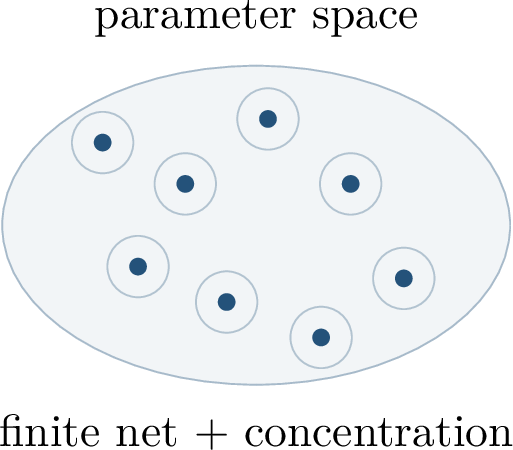
The reference notes emphasize the same idea in game-theoretic language. If a generator can approximate point masses, then a mixed generator strategy can represent the empirical data distribution. After discretizing the discriminator class and using a small-support equilibrium argument, a polynomial size mixture of generators can fool every discriminator in the restricted class. A sufficiently large network can then fold this mixture into one generator by using part of the latent randomness to select a component.
Theorem 0.49 (Restricted GAN equilibrium, informal). Assume the generator family can approximate point masses and the discriminator class has controlled complexity. Then there exists a generator mixture with polynomial-size support such that no \(D\in\mathcal{F}\) distinguishes its distribution from real data by more than \(\varepsilon\) in the restricted \(d_{\mathcal{F},\phi}\) sense. If the generator architecture is sufficiently large, the mixture can be implemented by one generator that uses latent randomness as a selector.
This result explains why restricted discriminators can generalize and why finite mixtures can be enough to fool a neural test class. It does not explain whether stochastic gradient methods find the equilibrium, whether the resulting samples are visually high quality, or whether all modes of the data distribution are covered. Those are additional questions about optimization, architecture, and the relation between the chosen distance and human or semantic notions of realism.
There is an important conceptual asymmetry here. A restricted discriminator distance can be small because \(Q\) is genuinely close to \(P\), or because the chosen \(\mathcal{F}\) is too weak to see the difference. The theorem controls generalization of the chosen game; it does not certify that the chosen game captures all aspects of the data distribution. In practice one therefore needs both statistical control and a discriminator architecture rich enough to encode the relevant features.
4.0.19 Game Theory Behind Approximate Equilibria↩︎
GANs are often described as two-player games. The relevant classical model is a finite zero-sum game. This finite model is not meant to describe the full continuous parameter space of neural networks. It is a bridge: after one discretizes generator and discriminator classes by approximation nets, one can apply finite-game theorems and then translate the resulting statements back to the neural setting with approximation error.
Definition 0.72 (Finite zero-sum game). A zero-sum game consists of two finite strategy sets \(\mathcal{U},\mathcal{V}\) and a payoff function \(F:\mathcal{U}\times\mathcal{V}\to\R\). Alice chooses \(u\in\mathcal{U}\), Bob chooses \(v\in\mathcal{V}\), Alice receives \(F(u,v)\), and Bob receives \(-F(u,v)\). Mixed strategies are probability distributions \(p\in\Delta(\mathcal{U})\) and \(q\in\Delta(\mathcal{V})\), with expected payoff \[\E_{u\sim p,\,v\sim q}F(u,v).\]
A payoff matrix is a concrete way to picture the game: \[\begin{array}{c|ccc} & v_1 & v_2 & v_3\\ \hline u_1 & 1 & -1 & 0\\ u_2 & -2 & 2 & 1\\ u_3 & 0 & -1 & 1 . \end{array}\] In the GAN analogy, generator strategies play the role of one player’s actions and discriminator strategies play the role of the other player’s actions.
Theorem 0.50 (von Neumann minimax theorem). For finite \(\mathcal{U},\mathcal{V}\), there is a value \(\eta\) such that \[\max_{p\in\Delta(\mathcal{U})} \min_{v\in\mathcal{V}} \E_{u\sim p}F(u,v) = \eta = \min_{q\in\Delta(\mathcal{V})} \max_{u\in\mathcal{U}} \E_{v\sim q}F(u,v).\] Alice can guarantee payoff at least \(\eta\), and Bob can hold Alice to payoff at most \(\eta\).
The minimax identity is a statement about mixed strategies. The order of play does not matter once each player is allowed to randomize optimally. In a GAN interpretation, a mixed generator strategy corresponds to drawing one generator from a distribution over generators and then drawing a sample from it. This is not the same as a single deterministic generator, but later we will see that a large enough neural generator can simulate such a mixture by using additional latent randomness.
Definition 0.73 (\(\varepsilon\)-approximate equilibrium). A pair of mixed strategies \((p,q)\) is an \(\varepsilon\)-equilibrium if no player can improve its expected payoff by more than \(\varepsilon\) by changing strategy unilaterally. Equivalently, for a maximizing Alice and minimizing Bob, \[\E_{p,q}F \ge \max_{p'}\E_{p',q}F-\varepsilon, \qquad \E_{p,q}F \le \min_{q'}\E_{p,q'}F+\varepsilon .\]
The chapter uses a small-support theorem to explain why one need not mix over all possible generators or discriminators.
Theorem 0.51 (Lipton-Markakis-Mehta). In any finite zero-sum game with \(m\) row strategies and \(n\) column strategies, for every \(\varepsilon>0\) there exist \(\varepsilon\)-optimal mixed strategies with support sizes \[O\!\left(\frac{\log n}{\varepsilon^2}\right) \quad\text{and}\quad O\!\left(\frac{\log m}{\varepsilon^2}\right).\]
Proof idea. Start from an exact minimax equilibrium. Sample \(s=O(\log n/\varepsilon^2)\) row strategies independently from Alice’s mixed strategy and let \(\widehat p\) be the empirical distribution on those samples. For any fixed column strategy, concentration shows that the payoff against \(\widehat p\) is close to the payoff against the original \(p\). A union bound over all \(n\) column strategies makes this true uniformly. The same subsampling argument applies to Bob’s strategy, with \(\log m\) in the support bound. ◻
After the discriminator class is discretized by a covering argument, the small-support theorem says that a small mixture of generator strategies can be enough to fool all discriminators in the net. The remaining modeling step is to implement the mixture as one generator.
The logarithmic support size is the crucial feature. If the discriminator net has many elements, a naive exact mixture might appear to require support comparable to the size of the net. The sampling proof shows that this is not necessary: a random empirical mixture of only \(O(\log n/\varepsilon^2)\) components preserves payoffs against all \(n\) pure discriminator strategies with high probability. This is one reason small-support equilibria are useful in GAN generalization theory.
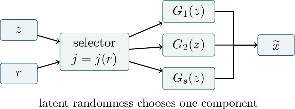
Equilibrium existence is not the same as training convergence. The toy game \[\min_x\max_y xy\] has an equilibrium at \((0,0)\), but simultaneous gradient descent-ascent gives \[x_{t+1}=x_t-\eta y_t,\qquad y_{t+1}=y_t+\eta x_t,\] which rotates around the saddle rather than moving directly into it.
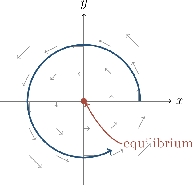
This distinction matters. The finite-sample and equilibrium results give structural reasons why restricted GAN objectives are not hopeless. They do not replace the analysis of the actual training dynamics used in neural-network optimization.
The bilinear example also explains why losses in adversarial training can look unlike ordinary supervised losses. In a single minimization problem, the negative gradient usually points locally toward lower objective value. In a game, one player’s descent direction is coupled to the other player’s ascent direction, and the resulting vector field may have rotational components. Stabilization methods for GANs can be viewed as attempts to control this coupled dynamics, but the existence of an equilibrium alone gives no such control.
4.0.20 Generative Priors for Inverse Problems↩︎
The last part of the chapter turns generative models from samplers into priors. Suppose an unknown signal \(x\in\R^d\) is observed through linear measurements \[b=Ax+\eta,\qquad A\in\R^{m\times d},\quad m\ll d ,\] where \(\eta\) is noise. Without structure, recovering arbitrary \(x\) requires \(A\) to have full column rank, so one needs at least \(d\) informative measurements. Compressed sensing shows that far fewer measurements suffice when \(x\) has structure.
The phrase prior here should be understood in a geometric sense. A prior restricts the set of plausible signals before the measurements are used. Classical compressed sensing uses the set of sparse vectors. Generative compressed sensing replaces this handcrafted set by the range of a trained network. The inverse problem is then no longer solved over all of \(\R^d\), but over a low-dimensional nonlinear model class.
Theorem 0.52 (Classical sparse compressed sensing). For a random Gaussian matrix \(A\), if \[m\gtrsim k\log(d/k),\] then with high probability a \(k\)-sparse vector \(x\) can be recovered from \(b=Ax\) by the convex program \[\widehat x = \argmin_{z\in\R^d}\left\lVert z \right\rVert_1 \qquad \text{subject to }Az=b .\] The recovery is stable under noise and model misspecification, in the sense that the estimate approximates the best \(k\)-sparse approximation to \(x\).
The proof is geometric. If there were two distinct \(k\)-sparse vectors that fit the same measurements, their difference would be \(2k\)-sparse and would lie nearly in the null space of \(A\). Random matrices of the right size make this unlikely.
This argument reveals the main role of randomness in the measurement matrix. The matrix does not need to preserve all directions in \(\R^d\); that would require \(m\) comparable to \(d\). It only needs to preserve the directions that arise as differences between two plausible signals. For sparse vectors, the set of such differences is the set of \(2k\)-sparse vectors.
Definition 0.74 (Sparse restricted isometry property). A matrix \(A\) satisfies the \((2k,\delta)\)-restricted isometry property if for every \(2k\)-sparse vector \(z\), \[(1-\delta)\left\lVert z \right\rVert_2^2 \le \left\lVert Az \right\rVert_2^2 \le (1+\delta)\left\lVert z \right\rVert_2^2 .\]
If two \(k\)-sparse candidates \(x,x'\) both approximately fit the data, then \(x-x'\) is \(2k\)-sparse. The RIP lower bound prevents \(A(x-x')\) from being too small unless \(x-x'\) is itself small. For Gaussian matrices, a standard covering and concentration argument gives the RIP with high probability when \(m\gtrsim k\log(d/k)\). This is the classical answer to the question: why can there not be two different sparse solutions that both fit the observations?
Natural images, however, are not literally sparse in the pixel basis. The chapter follows the idea of Bora, Jalal, Price, and Dimakis: replace the handcrafted sparsity model by the range of a trained generator [48].
Definition 0.75 (Generative compressed sensing). Let \(G:B_2^k(R)\to\R^d\) be a trained generator, and suppose \[x\approx G(z^\star),\qquad b=Ax+\eta .\] Estimate the latent vector by \[\widehat z = \argmin_{z\in B_2^k(R)} \left\lVert AG(z)-b \right\rVert_2, \qquad \widehat x=G(\widehat z).\]
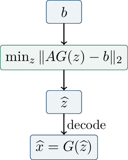
Theorem 0.53 (Compressed sensing with generative models). Let \(G:B_2^k(R)\to\R^d\) be \(L\)-Lipschitz. For a random Gaussian matrix \(A\), if \[m\gtrsim k\log(LR/\delta),\] then with high probability every approximate minimizer satisfies \[\left\lVert G(\widehat z)-x \right\rVert_2 \le 6\min_{z\in B_2^k(R)}\left\lVert G(z)-x \right\rVert_2 + 3\left\lVert \eta \right\rVert_2 + O(\delta).\]
The meaning of the theorem is direct. If \(x\) is close to the generator range and the measurements are not too noisy, then optimizing over the latent space recovers a signal close to \(x\). The number of measurements scales with the latent dimension \(k\), up to logarithmic factors, rather than directly with the ambient image dimension \(d\). For ReLU generators, the reference notes record the same phenomenon in a network-dependent form: the required number of Gaussian measurements is proportional to the latent dimension times network-complexity factors such as depth and logarithms of the ambient scale.
The error bound separates three unavoidable effects. The first term is the representation error: if the true signal is not close to the generator range, no method constrained to that range can recover it exactly. The second term is the measurement noise. The final \(O(\delta)\) term comes from the finite cover used in the proof and can be made smaller by increasing the number of measurements logarithmically. Thus the theorem does not say the generator prior is always correct; it says that, conditional on the prior being approximately correct, random measurements preserve enough information to recover within the natural errors.
The proof is the generative analogue of RIP. Instead of preserving distances between sparse vectors, the measurement matrix must preserve distances inside the generator range.
Definition 0.76 (Set-restricted eigenvalue condition). For a set \(S\subseteq\R^d\), a matrix \(A\) satisfies \(\mathrm{S-REC}(S,\gamma,\delta)\) if for all \(x,x'\in S\), \[\left\lVert A(x-x') \right\rVert_2 \ge \gamma\left\lVert x-x' \right\rVert_2-\delta .\]
Take \(S=G(B_2^k(R))\). A random matrix preserves pairwise distances on a finite cover of \(S\). Since \(G\) is Lipschitz, a cover of the latent ball induces a cover of the generator range. The inequality then extends from the finite cover to all latent points. Once S-REC holds, two points in the generator range that both fit the measurements cannot be far apart, except for the unavoidable errors caused by measurement noise and by the possibility that the true signal is not exactly in the range of \(G\).
This is exactly parallel to sparse RIP. In sparse compressed sensing, the set of relevant differences is \(\{x-x': x,x'\text{ are }k\text{-sparse}\}\). In generative compressed sensing, it is \[S-S=\{G(z)-G(z'): z,z'\in B_2^k(R)\}.\] The measurement matrix must be well conditioned only on this difference set. The Lipschitz assumption allows the size of a cover of \(S-S\) to be controlled by the latent dimension \(k\), which is why the measurement bound depends on \(k\) rather than directly on the ambient dimension \(d\).
Image inpainting is a concrete example. Missing pixels can be modeled as linear measurements: the rows of \(A\) select the observed pixels. Solving for \(\widehat z\) chooses a generator output that agrees with the visible pixels and fills in the rest according to the learned image prior.
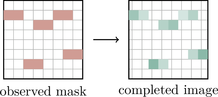
Generative priors are powerful but not magical. The true signal may not lie near the generator range. The latent optimization problem is nonconvex. Theory often assumes random measurements, while applications may use structured or adversarially missing observations. A biased generator can hallucinate plausible but incorrect details. The central tradeoff is between measurement consistency, prior realism, and semantic correctness.
Example 0.10 (A failure mode of a strong prior). Suppose the observed pixels of a face image are consistent with many possible identities, but the generator was trained on a dataset that underrepresents some identities. The optimization problem may find a latent code whose image matches the visible pixels and looks realistic, yet fills the missing region with biased or semantically wrong details. The measurement residual is small, but the reconstruction is not faithful. This illustrates why inverse problems with learned priors require both mathematical recovery guarantees and careful attention to the data distribution used to train the generator.
4.0.21 Connections and Outlook↩︎
GANs are one member of a broader family of deep generative models. The mathematical handle differs by family.
| Family | Training principle | Theoretical flavor |
|---|---|---|
| VAE | likelihood lower bound | variational inference |
| Normalizing flow | exact likelihood | invertible maps and Jacobians |
| GAN | adversarial testing | divergences and games |
| Diffusion | denoising score matching | stochastic processes |
| Autoregressive | chain-rule likelihood | sequential factorization |
This chapter adds five conceptual pieces to the monograph. First, the ideal GAN objective recovers Jensen-Shannon divergence. Second, the Wasserstein viewpoint replaces classification by transport geometry. Third, finite-sample GAN theory is meaningful only after restricting the discriminator class. Fourth, game theory explains why approximate equilibria can have small support, while also warning that equilibrium existence is not optimization convergence. Fifth, generators can be used outside sampling as nonlinear low-dimensional priors for inverse problems.
The common thread is that generative modeling is not only about producing images. It is also a meeting point for probability metrics, statistical generalization, game theory, optimization, and inverse problems. The same generator can be studied as a push-forward map, a player in a zero-sum game, a component of a distributional distance, or a low-dimensional prior. Keeping these views separate prevents a common confusion: a theorem about one view does not automatically solve the difficulties in the others.
The theory in this chapter leaves several important questions open. Which alternating algorithms converge in realistic nonconvex-nonconcave games? Which restricted discriminator distances best predict sample quality and mode coverage? How should reconstruction be certified when the generator itself was learned from finite data? These questions connect the present chapter to later themes on optimization, robustness, and representation learning.
Chapter Synthesis
A generator defines a push-forward distribution \(P_\theta=(G_\theta)_\#P_Z\); learning a generator is therefore a distribution-matching problem.
The ideal original GAN objective reduces to Jensen-Shannon divergence, but this divergence saturates when low-dimensional supports are disjoint.
Wasserstein GANs replace binary classification by transport geometry and rely on a Lipschitz critic to realize the Kantorovich-Rubinstein dual.
Finite-sample GAN theory becomes meaningful after restricting the discriminator class; uniform convergence then depends on discriminator complexity.
Small-support equilibrium arguments explain why mixtures of generators can fool a finite discriminator net, while training dynamics remain a separate issue.
In inverse problems, a trained generator can act as a nonlinear prior, with S-REC playing the role that RIP plays for sparse recovery.
Goodfellow et al., Generative Adversarial Nets (2014) [18]; Arjovsky, Chintala, and Bottou, Wasserstein GAN (2017) [42]; Gulrajani et al., Improved Training of Wasserstein GANs (2017) [43]; Arora, Ge, Liang, Ma, and Zhang, Generalization and Equilibrium in GANs (2017); Lipton, Markakis, and Mehta, Playing Large Games Using Simple Strategies (2003); Candes, Romberg, and Tao, Stable Signal Recovery from Incomplete and Inaccurate Measurements (2006); Donoho, Compressed Sensing (2006); Bora, Jalal, Price, and Dimakis, Compressed Sensing using Generative Models (2017) [48]. Useful surrounding reference materials include MIT 18.408, Telgarsky’s deep-learning-theory notes, Princeton COS 597G, Duke CS 590.2, EE227C, and Toronto CSC421.
5 Foundation Models and Emergent Mechanisms↩︎
5.0.1 From Learned Functions to Learned Algorithms↩︎
Earlier chapters asked how neural networks approximate functions, how gradient methods optimize them, and why they may or may not generalize. Transformers add a new phenomenon. A pretrained model can adapt to a task described inside the prompt even though its parameters remain fixed. The examples in the context act like temporary training data, and the forward pass acts like a task-specific learning procedure. This phenomenon became empirically visible in large language models, where a model trained only for next-token prediction can use a few demonstrations in the prompt to perform a new classification, translation, arithmetic, or reasoning pattern [49].
For theory, the striking point is not merely that prompts affect predictions. Every conditional model changes its output when the input changes. The more specific claim is that the prompt can specify an algorithmic problem: from a finite set of examples, infer a hidden rule and apply it to a query. The model parameters store a general procedure learned during pretraining, whereas the activations store the task-specific information extracted from the current prompt. In-context learning therefore sits between representation learning and algorithm learning.
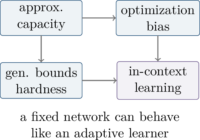
Definition 0.77 (In-context learning). Let \(C_n=((x_i,y_i))_{i=1}^n\) be a context of examples and let \(x_\star\) be a query. A fixed predictor \(T_\theta\) performs in-context learning when it outputs \[\widehat y_\star=T_\theta(C_n,x_\star)\] without changing the parameter vector \(\theta\). The prompt supplies the task instance; the forward pass adapts to it.
This definition is intentionally broad. The context might be a list of supervised examples, a natural-language instruction, a partial computation, or a mixture of all three. What makes the phenomenon theoretically interesting is that the same conditional model is used for many tasks. The model must infer which rule is relevant from the evidence in the prompt.
Two kinds of adaptation should be kept separate. During pretraining, the parameters \(\theta\) are updated across many sequences and many tasks. During in-context learning, \(\theta\) is frozen; only the hidden states change as the prompt is processed. A useful mental model is that pretraining learns a family of possible procedures, and the prompt selects or instantiates one of them. This separation is what makes ICL different from ordinary fine-tuning.
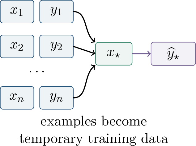
Transformers are particularly well suited to this view because self-attention compares every token with previous tokens, assigns data-dependent weights, and then aggregates information. In a causal language model, this aggregation is online: token \(t\) can use tokens \(1,\ldots,t\), but not future tokens. Each layer can refine the representation, so depth can behave like computation time.
The same architecture also makes the analysis nontrivial. The function computed at a query token depends on all earlier tokens through attention weights, and those weights themselves depend on the hidden representations produced by previous layers. A transformer is therefore not simply applying a fixed kernel to the prompt. It repeatedly builds new features, uses those features to decide what to read, and then writes the result back into the residual stream.
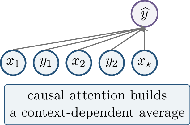
The guiding question for this chapter is:
When does a pretrained transformer implement a learning algorithm inside its forward pass?
The answer has three parts. Architecture tells us how attention and residual streams process the prompt. Expressivity tells us which sequence maps and learning rules a transformer can represent. Statistics tells us when pretraining over tasks leads to generalization to a new prompt.
5.0.2 Transformer Mechanics↩︎
Let \(z_{1:T}\) be a sequence of tokens. Autoregressive pretraining optimizes next-token prediction: \[\min_\theta\; \E_{z_{1:T}\sim\mathcal{D}} \left[ -\sum_{t=1}^{T-1} \log p_\theta(z_{t+1}\mid z_{\le t}) \right].\] In-context learning is not a different training rule. It is a way of using the learned conditional distribution. A prompt may encode a dataset, a rule, or a partial computation, and next-token prediction asks the model to continue the sequence consistently. The transformer architecture introduced by Vaswani et al. [19] is designed to make this conditional distribution highly context-sensitive while remaining parallelizable during training.
There are three ingredients to keep in view. Token embeddings turn discrete symbols or structured inputs into vectors. Positional information lets the network distinguish the first example from the tenth example and the query from the demonstrations. Self-attention then allows a token to retrieve information from other tokens using learned similarity scores. Feed-forward layers and residual connections transform and preserve the information that has been retrieved.
5.0.2.1 Scaled Dot-Product Attention
Let \(H\in\R^{T\times d}\) be the matrix of token representations in one layer. For one attention head, \[Q=HW_Q,\qquad K=HW_K,\qquad V=HW_V,\] and the output is \[\operatorname{Attn}(H) = \softmax\!\left(\frac{QK^\top}{\sqrt{d_k}}+M\right)V.\] The matrix \(QK^\top\) contains similarity scores between query and key representations. The mask \(M\) enforces causal structure. After softmax, the row \(A_{t\cdot}\) is a probability vector describing which previous tokens token \(t\) reads from.
The factor \(1/\sqrt{d_k}\) is a normalization. If query and key coordinates have roughly unit variance, then an unnormalized dot product has variance of order \(d_k\). Large dot products can push the softmax into a nearly one-hot regime early in training, making gradients poorly scaled. Dividing by \(\sqrt{d_k}\) keeps the logits at a comparable scale as the head dimension changes.
It is useful to read the formula row by row. For token \(t\), the vector \(q_t\) is a request, each \(k_j\) is an address, and each \(v_j\) is the stored content. The attention weights say which addresses match the request, and the output is the corresponding weighted average of contents. This is the content-addressable memory interpretation of attention.
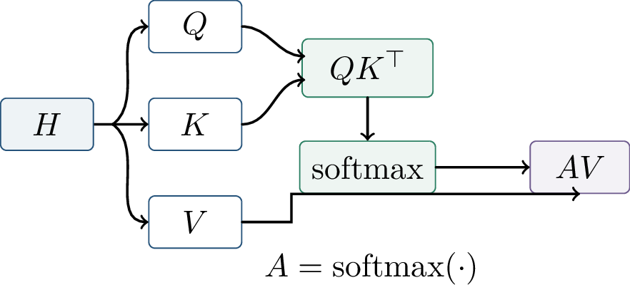
Definition 0.78 (Causal mask). For an autoregressive transformer, token \(t\) is only allowed to attend to positions \(1,\ldots,t\). Equivalently, the attention weights satisfy \[A_{tj}=0\qquad\text{for }j>t.\] This makes the transformer a learned online algorithm over the prompt.
The mask is a structural constraint, not a learned preference. It guarantees that the conditional distribution factors autoregressively: \[p_\theta(z_{1:T}) = \prod_{t=1}^T p_\theta(z_t\mid z_{<t}).\] Without the mask, a training token could read the future token it is supposed to predict, turning next-token prediction into a leakage problem. With the mask, the representation at position \(t\) can be interpreted as the state of a sequential algorithm after processing the prefix \(z_{\le t}\).
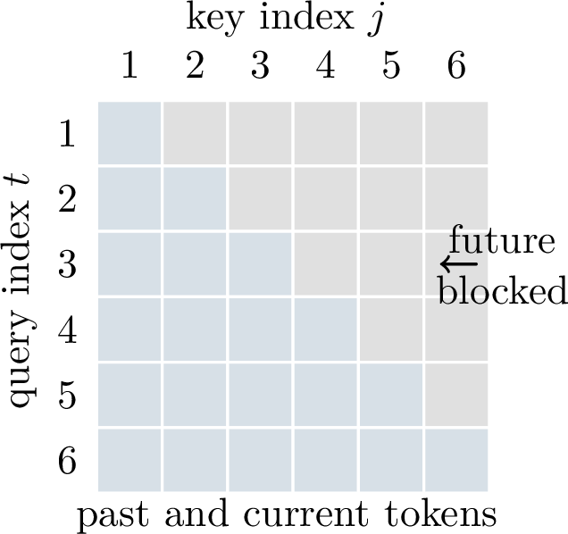
5.0.2.2 Blocks and Heads
A transformer block alternates communication across positions with local nonlinear transformations. In the simplified residual form used in the slides, \[U^\ell = H^\ell+\operatorname{MHA}(H^\ell), \qquad H^{\ell+1}=U^\ell+\operatorname{MLP}(U^\ell).\] The residual stream preserves old information, attention moves information between positions, and MLPs transform each token representation.
This decomposition is conceptually important for in-context learning. The attention sublayer is where the query token can read from examples in the prompt. The MLP sublayer is where the representation at each position can be nonlinearly rewritten. The residual connection prevents each sublayer from having to reconstruct all useful information from scratch; instead, layers can add small computational updates to a persistent state.
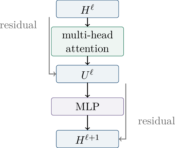
Multi-head attention repeats the attention operation several times with different learned projections. Heads are not independent learners, but they give the model several simultaneous memory reads. One head may retrieve a label, another may compare features, and the output projection recombines these partial computations.
From a theoretical standpoint, heads provide parallel relational features. For instance, in a prompt of input-output pairs, one head can attend from the query to input tokens similar to \(x_\star\), while another can route the corresponding labels, and a later layer can combine those retrieved quantities. This picture is schematic, but it explains why multi-head attention is often described as several learned views of the same context.
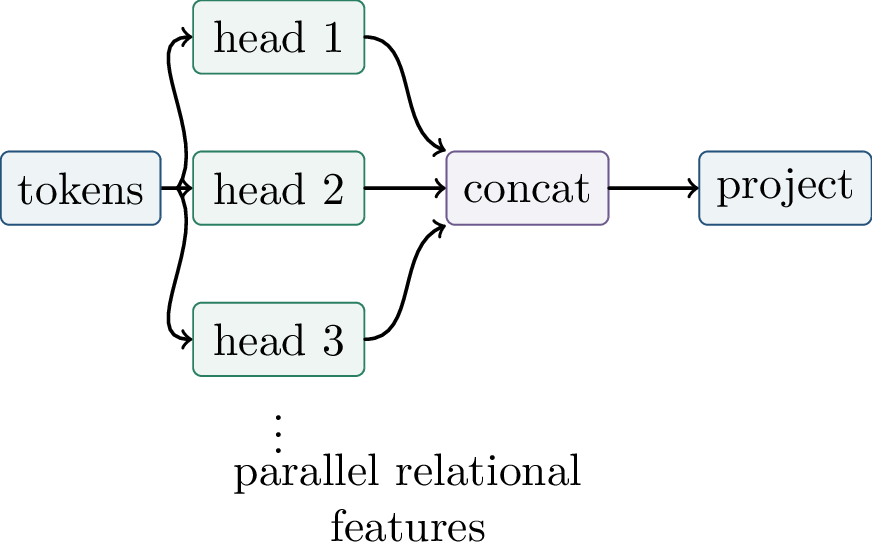
5.0.3 Expressivity and Attention↩︎
For a query token \(i\), one attention head computes \[h_i^+=\sum_{j\le i}a_{ij}v_j, \qquad a_{ij} = \frac{\exp(q_i^\top k_j/\sqrt{d_k})}{\sum_{r\le i}\exp(q_i^\top k_r/\sqrt{d_k})}.\] This formula is a learned, data-dependent smoother. The value vectors \(\{v_j\}\) are averaged using weights determined by the current representations.
This view deliberately resembles nonparametric regression. A kernel smoother predicts at a query by averaging nearby training values. Attention does something analogous, but both the notion of nearness and the objects being averaged are learned and context-dependent. A head can therefore behave like nearest-neighbor retrieval in one layer and like a more abstract feature matching mechanism in a later layer.
Self-attention is a learned kernel smoother whose kernel is computed from the current sequence representation: \[K_\theta(i,j;H)=\exp(q_i^\top k_j/\sqrt{d_k}).\] Unlike a fixed kernel, \(K_\theta\) changes with the sequence and with the layer.
This data dependence is the basic mechanism behind prompt-conditioned computation. The prompt changes the keys and values available to later tokens, and therefore changes the function computed at the query position.
One should not overinterpret the word “kernel.” Classical kernels are fixed functions of the inputs, while attention kernels are functions of hidden states that have already mixed information from the entire prefix. Thus attention can implement iterative algorithms: a first layer may build a feature used for matching, and a later layer may match using that newly constructed feature.
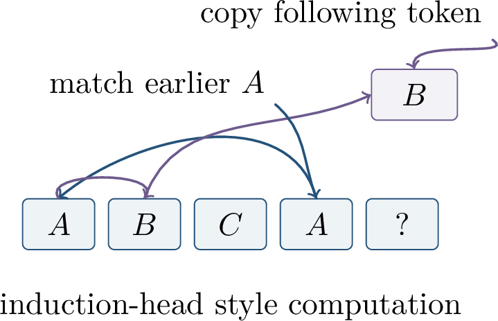
Mechanistic studies of in-context learning have found induction heads in trained transformer language models. The diagram is schematic, but it captures the algorithmic flavor: a head can use content matching to retrieve a past continuation and copy it into the prediction path.
Example 0.11 (Induction in a repeated pattern). Consider the token sequence \[A,\;B,\;C,\;A,\;?\] and suppose the model has learned that when a current token matches a previous token, the next token after the earlier occurrence is a plausible continuation. At the final position, a head can attend from the second \(A\) to the first \(A\), retrieve the fact that \(B\) followed it, and route information toward predicting \(B\). This is not a proof of how every model works, but it is a minimal example of how attention can implement a symbolic-looking operation through vector similarity and copying.
Theorem 0.54 (Transformer universality, informal). With positional encodings and sufficient width and depth, transformer networks can approximate broad classes of continuous sequence-to-sequence maps on compact domains.
Attention supplies global interaction among positions, feed-forward layers supply nonlinear local transformations, and positional information breaks permutation symmetry when order matters. This is an expressivity theorem: it says what can be represented, not why pretraining finds a useful representation.
The distinction between expressivity and learnability is essential. A universality theorem says that some parameter setting can approximate the desired sequence map on a compact domain. It does not say that stochastic gradient descent will find that parameter setting, that the representation is robust to longer contexts, or that the approximation extrapolates beyond the domain used in the theorem. In this chapter, universality is a possibility result, not a training guarantee.
Theorem 0.55 (Universal in-context learners, informal). For suitable token encodings, a transformer can approximate continuous learning rules of the form \[\mathcal{A}:\bigl((x_1,y_1),\ldots,(x_n,y_n),x_\star\bigr)\mapsto \widehat y_\star\] on compact prompt domains.
The learning rule \(\mathcal{A}\) might be ridge regression, a nearest-neighbor rule, a small number of gradient steps, a Bayesian posterior mean, or another continuous algorithm after suitable encoding. The theorem says that a transformer can approximate the map from the entire prompt to the output of that algorithm. It does not require the transformer to explicitly store a parameter vector \(w\) in a human-readable way; the intermediate computation may be distributed across many hidden coordinates.
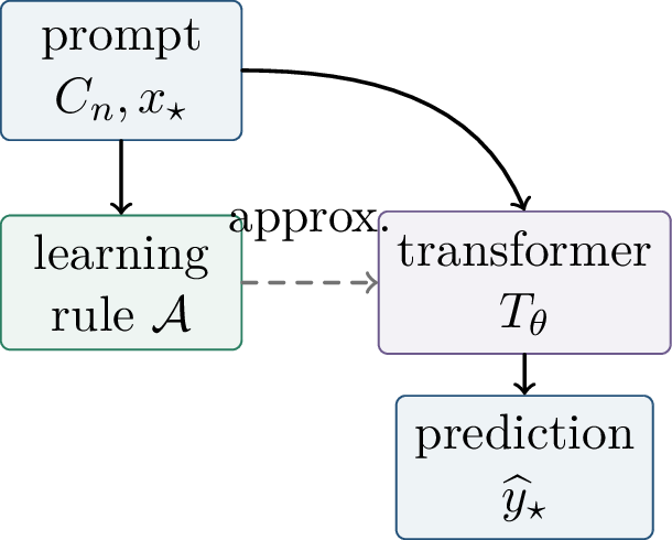
The expressivity landscape has three levels. Attention can route information by content-based lookup. Transformers can represent many formal algorithms, though robustness under finite precision is subtle. In-context learning can solve new tasks under a task-distribution assumption, but extrapolation outside the pretraining mixture remains a separate statistical challenge.
This hierarchy will guide the rest of the chapter. First we identify simple algorithms that attention layers can implement. Then we ask which of these algorithms are statistically optimal for a task distribution. Finally we separate task-distribution generalization from out-of-distribution extrapolation.
5.0.4 In-Context Learning as an Algorithm↩︎
Many theory papers study prompts generated by a hidden linear rule, \[w\sim\Pi,\qquad x_i\sim\mathcal{D}_x,\qquad y_i=x_i^\top w+\xi_i.\] Given \(C_n=((x_i,y_i))_{i=1}^n\) and a query \(x_\star\), the goal is to predict \[y_\star=x_\star^\top w.\] This model deliberately removes language semantics. It isolates the algorithmic question: can a transformer infer an unknown rule from examples in the context? This is the setting of several recent theoretical studies of in-context learning, including the simple-function-class experiments of Garg et al. [50] and the gradient-descent interpretation of von Oswald et al. [51].
Linear regression is useful because the statistically natural answers are known. With no noise and enough well-conditioned examples, least squares recovers the hidden vector. With Gaussian priors and Gaussian noise, ridge regression is the posterior mean. With finite computation, gradient descent gives an iterative approximation. Thus one can ask a precise mechanistic question: which of these algorithms does a trained transformer emulate?
Let \(X\in\R^{n\times d}\) have rows \(x_i^\top\), and let \(y=(y_1,\ldots,y_n)\). Ridge regression computes \[\widehat w_\lambda = (X^\top X+\lambda I)^{-1}X^\top y, \qquad \widehat y_\star=x_\star^\top\widehat w_\lambda .\] The case \(\lambda=0\) is least squares when the design is identifiable. Positive \(\lambda\) provides shrinkage, which controls noise and collinearity. The theoretical question is whether a transformer can approximate this map from the prompt alone.
The map is nonlinear in the prompt even though the target function is linear in \(x_\star\). The inverse \((X^\top X+\lambda I)^{-1}\) depends on all examples. Consequently, a model that performs ridge regression in context is not merely fitting a fixed linear predictor; it is computing a data-dependent estimator inside its activations. This is why linear regression is already a nontrivial test of algorithmic ICL.
Gradient descent gives another algorithmic target. For squared loss \[L(w)=\frac{1}{2n}\left\lVert Xw-y \right\rVert^2,\] the update is \[w_{t+1} = w_t-\eta\frac{1}{n} X^\top(Xw_t-y).\] The update is built from sums of products involving \(x_i\), \(y_i\), and the current iterate \(w_t\). Attention layers are naturally good at weighted summation, so they can resemble steps of an optimization algorithm.
Starting from \(w_0=0\), the first step is especially transparent: \[w_1 = \eta\frac{1}{n} X^\top y = \eta\frac{1}{n}\sum_{i=1}^n y_i x_i .\] The prediction after one step is \[x_\star^\top w_1 = \eta\frac{1}{n}\sum_{i=1}^n y_i\,\left\langle x_\star,x_i \right\rangle.\] This has exactly the form of a similarity-weighted aggregation over the context. The attention analogy is therefore not superficial: the query \(x_\star\) scores examples through inner products and aggregates their labels through the values.
Lemma 0.24 (Linear attention gradient-descent step, informal). With suitable encodings, a linearized attention layer can produce the statistic \[\frac{1}{n}\sum_{i=1}^n y_i x_i\] and form the first gradient step from \(w_0=0\) for linear regression.
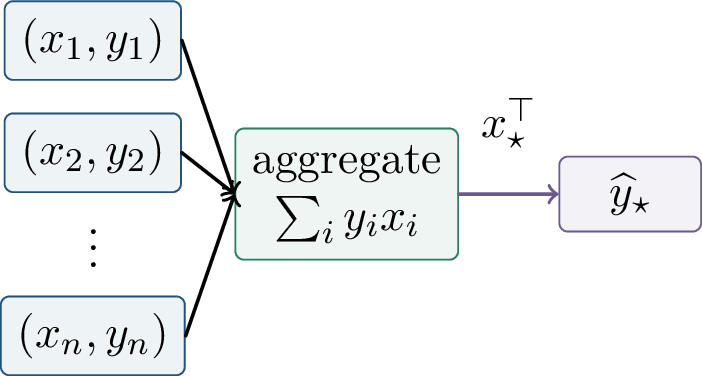
Proof idea. Store \(x_i\) in key and value features and store \(y_i\) in value features. The query token collects a context statistic such as \(\sum_i y_i x_i\). The output projection combines this statistic with \(x_\star\) to produce \(\widehat y_\star\). Repeating the same pattern with a representation of the current iterate gives later gradient steps. ◻
The proof idea hides several engineering details that matter in formal constructions. The prompt must encode both \(x_i\) and \(y_i\) so that the layer can form products or bilinear features. The query representation must carry \(x_\star\). Residual coordinates must preserve the current iterate from one layer to the next. MLP sublayers can be used to form nonlinear features and to update the representation after attention has aggregated the necessary statistics.

Theorem 0.56 (Preconditioned gradient descent, informal). For linear regression prompts, trained transformer architectures can implement updates resembling \[w_{t+1}=w_t-\eta P_t X^\top(Xw_t-y)/n,\] where \(P_t\) acts like a learned preconditioner adapted to the task distribution.
A good preconditioner accelerates convergence in ill-conditioned problems. This connects in-context learning to optimization theory: the model may learn an optimizer, not only an estimator. The learned rule depends strongly on the pretraining distribution. For simple function classes beyond dense linear regression, theory and experiments ask whether transformers recover the appropriate classical procedures: coordinate selection for sparse linear functions, recursive partitioning for decision trees, and other simple algorithmic templates.
Preconditioning is also a place where the task distribution enters. If pretraining examples usually have covariance \(\Sigma\), then a rule that rescales directions according to \(\Sigma^{-1}\) may converge much faster than plain gradient descent on typical prompts. Under a different covariance structure, the same learned preconditioner may be suboptimal or even harmful. This is a recurring theme: in-context learning is algorithmic, but the algorithm is shaped by the distribution on which it was learned.
5.0.5 A Statistical View↩︎
In-context learning is naturally modeled as learning over tasks. Let \[\tau\sim\Pi,\qquad (x_i,y_i)_{i=1}^n,(x_\star,y_\star)\sim\mathcal{D}_\tau .\] Pretraining minimizes a task-averaged loss \[\E_{\tau,C_n,(x_\star,y_\star)} \ell\bigl(T_\theta(C_n,x_\star),y_\star\bigr).\] The task prior \(\Pi\) determines what can be inferred from a few examples. Generalization across prompts and generalization across tasks are therefore different problems.
This task-level formulation is the statistical counterpart of the algorithmic view. The algorithm implemented by the transformer is useful only relative to a population of tasks. If \(\Pi\) puts mass on linear functions, then a least-squares-like procedure may be appropriate. If \(\Pi\) puts mass on decision trees, sparse functions, or natural-language transformations, the right procedure may be different. A prompt is informative because it narrows down the latent task drawn from \(\Pi\).
5.0.5.1 Bayesian Posterior Prediction
Under a Bayesian task prior, the optimal predictor is the posterior predictive distribution \[\require{physics} p(y_\star\mid C_n,x_\star) = \int p_\tau(y_\star\mid x_\star)\, p(\tau\mid C_n)\,\dd\tau .\] If pretraining samples tasks from \(\Pi\), then an optimal sequence model for the pretraining distribution approximates this posterior predictive rule. This is the sense in which in-context learning can be viewed as amortized Bayesian inference.
The word “amortized” means that the costly inference rule is learned once during pretraining and then reused at test time. At test time the model does not explicitly run Bayes’ rule over a written-down prior. Instead, its forward pass approximates the input-output map that Bayes’ rule would define under the pretraining distribution. This viewpoint explains both the strength and the fragility of ICL: it can be very efficient on familiar task families, but it inherits the assumptions encoded by the pretraining mixture.
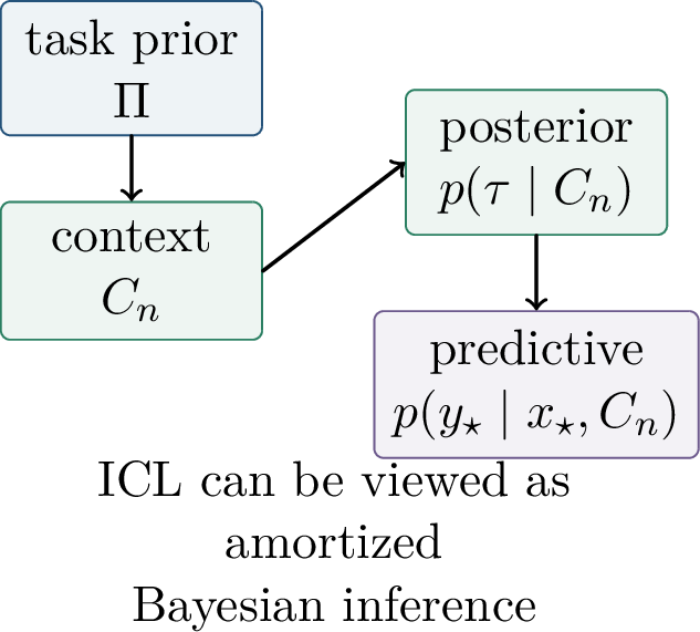
Example 0.12 (Linear-Gaussian tasks). Assume \[w\sim N(0,\tau^2 I),\qquad y_i=x_i^\top w+\xi_i,\qquad \xi_i\sim N(0,\sigma^2).\] Then the posterior mean prediction is \[\E[y_\star\mid C_n,x_\star] = x_\star^\top (X^\top X+\lambda I)^{-1}X^\top y, \qquad \lambda=\sigma^2/\tau^2 .\] Thus Bayes prediction coincides with ridge regression.
This example also clarifies the role of the regularization parameter. A larger noise variance \(\sigma^2\) increases \(\lambda\), causing stronger shrinkage toward the prior mean \(0\). A larger prior variance \(\tau^2\) decreases \(\lambda\), allowing the data to determine \(w\) more aggressively. In the ICL interpretation, a model trained on many such tasks can learn not only to fit the examples, but also how much to trust them.
5.0.5.2 Algorithm Selection
Prompts may come from a mixture of task families. For example, one task may be linear, another sparse, and another tree-structured. The prompt must first identify which latent family is appropriate, and then the model must apply the matching rule. This is model selection inside the context.
The selection step is statistical before it is computational. If the examples in a short prompt are compatible with several families, then no deterministic algorithm can identify the family with certainty without additional prior information. The best predictor averages or hedges according to posterior probabilities over task families. Only after the family becomes sufficiently clear should the model specialize to a family-specific rule.
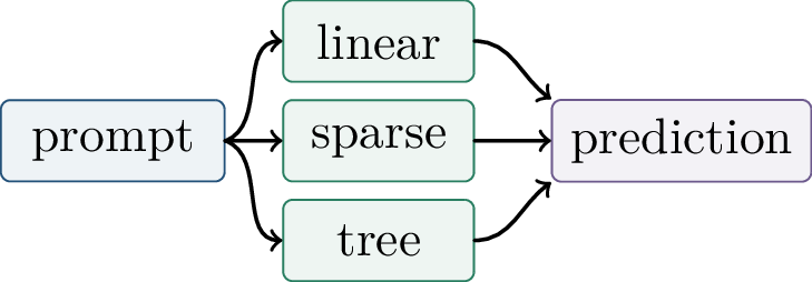
Mixture models clarify both the promise and the limitation. Wider pretraining mixtures can improve task identification; rare task families need enough mass to be learned; and interpolation between families is not automatic.
The last point is often missed. Training on two task families does not automatically imply competence on every meaningful interpolation between them. If the low-density region between the families is rarely observed during pretraining, the model may have little evidence for which algorithm should apply there. This is a task-level version of distribution shift.
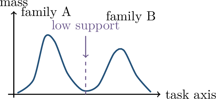
5.0.6 Generalization and Limits↩︎
There are at least three axes of generalization. A transformer can be fluent at token-level language modeling, yet fail to infer the correct rule from a short prompt. Prompt-level sample efficiency asks how many examples are needed inside the context. Task-level transfer asks whether the learned algorithm extends to a new task family.
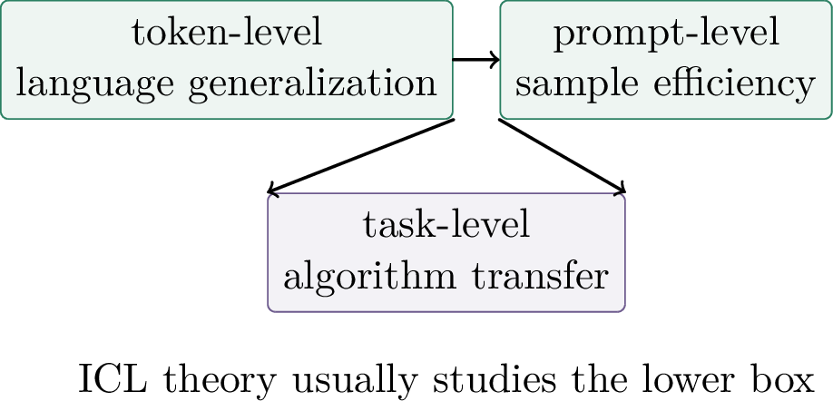
The sample complexity knobs include the context length \(n\), the ambient dimension \(d\), the noise level \(\sigma\), the task prior \(\Pi\), and the model’s capacity and depth. For linear-Gaussian tasks, a useful decomposition has the schematic form \[\mathcal{E}_{\mathrm{pred}} \approx \mathcal{E}_{\mathrm{stat}}(n,d,\sigma) + \mathcal{E}_{\mathrm{alg}} .\] The first term is irreducible statistical difficulty under the task prior; the second is the error from approximating or implementing the algorithm inside the transformer.
This decomposition is not a formal theorem as written, but it is a useful organizing principle. Even a Bayes-optimal predictor has statistical error when the context is short or noisy. A finite transformer adds approximation and optimization error because it may only partially implement the desired procedure. Empirical ICL failures can arise from either source: the prompt may not contain enough evidence, or the model may fail to use the evidence that is present.

From a short prompt alone, many task rules can agree on all observed examples but disagree on the query. The prior over tasks is therefore doing real statistical work. A learned in-context algorithm can be brittle under out-of-distribution prompts; finite context length limits the evidence shown to the model; finite depth limits the number of computation steps that can be simulated; and finite precision can matter when representing exact algorithms.
For any finite context \(C_n\), there may be many functions that agree on all observed pairs and disagree at \(x_\star\). Thus the prompt alone rarely identifies the task without assumptions. What looks like “reasoning from the prompt” is always reasoning from the prompt together with an implicit prior learned during pretraining. This is not a weakness of the Bayesian view; it is the statistical content of in-context learning.
The connections to earlier chapters are direct. Approximation theory asks which sequence algorithms transformers can represent. Optimization theory asks how pretraining installs optimizer circuits. Implicit regularization asks which algorithm is selected by training dynamics. Generalization theory asks for task-level bounds. SQ lower bounds warn that prompts may hide hard structure. Robustness theory warns that adversarial prompts can manipulate the inferred task.
5.0.7 Illustrative Analysis and Outlook↩︎
Example 0.13 (A one-dimensional small-scale exercise). Suppose \(d=1\), \(y_i=wx_i\), there is no noise, and the prompt gives two examples. The least-squares estimate is \[\widehat w = \frac{x_1y_1+x_2y_2}{x_1^2+x_2^2}, \qquad \widehat y_\star=x_\star\widehat w .\] This formula is a context-dependent computation. A transformer does not change its weights; it must represent the computation in activations.
The main takeaways are these. First, self-attention is content-based memory access with causal order and learned nonlinear updates. Second, for simple task families, transformer layers can implement recognizable algorithms such as least squares, ridge regression, gradient descent, and preconditioned gradient descent. Third, the task prior induced by pretraining determines what can be inferred from a short prompt.
Important theory questions remain open. Which training dynamics produce gradient-descent-like in-context circuits? Can we prove task extrapolation outside the pretraining mixture? What is the right complexity measure for an in-context algorithm? How do chain-of-thought and test-time computation change the theory? Can mechanistic interpretability certify an in-context algorithm inside a model?
Chapter Synthesis
In-context learning is adaptation through activations rather than through parameter updates.
Scaled dot-product attention implements content-addressable memory: queries read values through learned query-key similarities.
Causal masking turns a transformer into an online sequence model, so each position can depend only on the prefix.
Attention can be viewed as a learned, data-dependent kernel smoother, and transformer expressivity results show that many sequence algorithms can be represented.
Linear regression prompts expose the algorithmic content of ICL: attention layers can resemble gradient steps, ridge regression, or learned preconditioned optimization.
The statistical view treats prompts as evidence about a latent task. The pretraining task distribution determines which algorithms are selected and where distribution shift appears.
Foundational references include Vaswani et al., Attention Is All You Need [19]; Brown et al., Language Models are Few-Shot Learners [49]; and Olsson et al., In-context Learning and Induction Heads. Theory references include Xie et al., An Explanation of In-context Learning as Implicit Bayesian Inference; Garg et al., What Can Transformers Learn In-Context? [50]; Akyurek et al., What learning algorithm is in-context learning?; von Oswald et al., Transformers learn in-context by gradient descent [51]; Ahn et al., Transformers learn to implement preconditioned gradient descent; Bai et al., Transformers as Statisticians; Yadlowsky, Doshi, and Tripuraneni, Pretraining data mixtures enable narrow model selection; and Furuya, de Hoop, and Peyre, Transformers are Universal In-context Learners.
Transformer theory turns deep learning theory from studying learned functions into studying learned algorithms. The next natural topics are generative sequence models with richer test-time computation, diffusion and flow matching, and mechanistic interpretability methods that try to locate the learned algorithms inside trained networks.
5.0.8 From Generative Games to Learned Transport↩︎
Generative modeling asks for a mechanism that produces new samples whose law is close to the unknown data distribution \(p_{\mathrm{data}}\). Earlier generative approaches often emphasized either an adversarial test, as in GANs, or an invertible change of variables, as in normalizing flows. Diffusion models and flow matching take a different route: they introduce a path of distributions that connects a simple law, usually Gaussian noise, to the data law, and then learn the local dynamics along that path.
This path-based viewpoint is useful because it replaces one very hard global problem by many easier local problems. Matching \(p_{\mathrm{data}}\) directly would require understanding a complicated high-dimensional distribution. Instead, diffusion and flow methods ask the model to learn what should happen at a point \(x\) and a time \(t\): should the sample move toward a denoised version, follow a probability-flow velocity, or travel along a prescribed interpolation? The learned object is therefore a vector field rather than an explicit density.
The guiding question for this chapter is:
How can a neural network learn a high-dimensional transport map without explicitly computing the data density?
The answer is that the model need not represent the density itself. It can instead learn local vector fields: denoising directions, scores, or velocities. Once the field is learned, sampling becomes a numerical integration problem.
This is the conceptual bridge to the rest of the monograph. Approximation theory asks whether neural networks can represent the required time-dependent field. Optimization asks whether the supervised regression objectives find it. Generalization asks whether finite data and finite time samples are enough. Numerical analysis asks how errors accumulate when the learned dynamics are integrated.
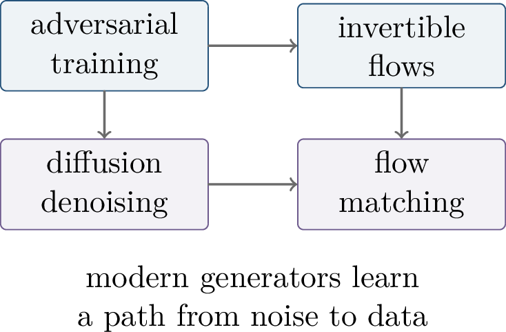
Definition 0.79 (Denoising generator). A diffusion model chooses a forward corruption process that maps \(x_0\sim p_{\mathrm{data}}\) to noisy variables \[x_t \approx \alpha_t x_0+\sigma_t\varepsilon, \qquad \varepsilon\sim \mathcal{N}(0,I),\] and learns a reverse-time rule that removes noise step by step. Training is supervised by corrupted data; sampling starts from noise and follows the learned reverse dynamics.
The forward process is not learned. It is a mathematical device that creates training pairs: a clean data point, a noise level, and a corrupted observation. The learned model is trained to reverse this device locally. This is why diffusion training can be formulated as ordinary supervised regression even though the final task is unsupervised sample generation.
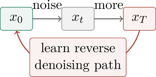
Definition 0.80 (Continuous transport and flow matching). Let \(X_0\sim p_{\mathrm{base}}\) be a base sample and \(X_1\sim p_{\mathrm{data}}\) a data sample. Flow matching specifies a continuous path \(X_t\) from base to data and learns a time-dependent velocity field \[\require{physics} \frac{\dd X_t}{\dd t}=v_t(X_t).\] The generator is obtained by solving this ODE forward from \(t=0\) to \(t=1\).
Flow matching changes the direction of construction. Rather than starting from a stochastic noising process and deriving a reverse-time score, it chooses a path from \(p_{\mathrm{base}}\) to \(p_{\mathrm{data}}\) and regresses the velocity of that path directly. The design question becomes: which path produces a velocity field that is easy to learn and easy to integrate?
The chapter has three layers. First, we review the discrete DDPM construction. Second, we pass to continuous-time score SDEs and probability-flow ODEs. Third, we formulate flow matching as direct velocity regression and compare the resulting path design and solver questions.
5.0.9 Discrete Diffusion↩︎
5.0.9.1 Forward Noising
DDPMs define a fixed forward Markov chain that gradually destroys the data signal. The formulation below follows the denoising diffusion probabilistic model framework of Ho, Jain, and Abbeel [20]. For a variance schedule \(\beta_t\in(0,1)\), \[q(x_t\mid x_{t-1}) = \mathcal{N}\!\left(\sqrt{1-\beta_t}\,x_{t-1},\,\beta_tI\right).\] Let \(\bar\alpha_t=\prod_{s=1}^t(1-\beta_s)\). Iterating the Gaussian transition gives the closed-form marginal \[q(x_t\mid x_0) = \mathcal{N}\!\left(\sqrt{\bar\alpha_t}\,x_0,\,(1-\bar\alpha_t)I\right).\] Thus \(x_t\) can be sampled directly as \[x_t=\sqrt{\bar\alpha_t}\,x_0+\sqrt{1-\bar\alpha_t}\,\varepsilon, \qquad \varepsilon\sim\mathcal{N}(0,I).\] The Markov chain is known; the difficult object is the reverse chain.
The closed-form marginal is obtained by repeatedly composing Gaussian affine transitions. Each step multiplies the previous signal by \(\sqrt{1-\beta_t}\) and adds independent Gaussian noise. Products of the signal coefficients give \(\sqrt{\bar\alpha_t}\), while the accumulated independent noise terms combine into an isotropic Gaussian with variance \(1-\bar\alpha_t\). This formula is what allows training to sample an arbitrary time \(t\) directly instead of simulating all earlier noising steps.
5.0.9.2 Denoising Parameterizations
For a generic continuous notation \[x_t=\alpha_t x_0+\sigma_t\varepsilon,\] there are several equivalent objects that can be predicted by a neural network. It may predict the noise \(\varepsilon\), the clean signal \(x_0\), or the score \(\nabla_x\log p_t(x_t)\). The link is supplied by Tweedie’s formula: \[\E[x_0\mid x_t=x] = \frac{x+\sigma_t^2\nabla_x\log p_t(x)}{\alpha_t}.\] In words, the posterior mean denoiser is the noisy point plus a score correction, scaled back by \(\alpha_t\). Noise prediction is often numerically stable, whereas score prediction exposes the continuous-time theory.
The simplified DDPM loss samples a time \(t\), data \(x_0\), and Gaussian noise \(\varepsilon\), forms \(x_t=\alpha_t x_0+\sigma_t\varepsilon\), and trains \[\min_\theta \E\,\left\lVert \varepsilon_\theta(x_t,t)-\varepsilon \right\rVert^2.\] The regression target is known because we created the corruption. At the population optimum, the network learns the conditional mean of the noise, hence the direction that removes corruption.
More precisely, for squared loss the optimal predictor is \[\varepsilon_\theta^\star(x,t)=\E[\varepsilon\mid X_t=x].\] Thus the model is not asked to recover the exact noise realization from one noisy observation; that would generally be impossible. It is asked to predict the best mean-square denoising direction. This distinction matters because it connects the DDPM loss to conditional expectation and, through the score identity below, to likelihood gradients.
5.0.9.3 Reverse Sampling
Sampling uses learned reverse conditionals \[p_\theta(x_{t-1}\mid x_t) = \mathcal{N}\!\left(\mu_\theta(x_t,t),\,\Sigma_t\right)\] to transform \(x_T\sim\mathcal{N}(0,I)\) into a sample near the data distribution. The learned mean points toward higher data likelihood, while the variance term keeps the reverse chain compatible with the noising process and avoids premature collapse.
The reverse conditional is difficult because it depends on the unknown data distribution through the posterior \(q(x_{t-1}\mid x_t)\). The forward conditional \(q(x_t\mid x_{t-1})\) is chosen by us, but Bayes’ rule for going backward requires the marginal law of \(x_{t-1}\), which is induced by \(p_{\mathrm{data}}\). Diffusion modeling learns precisely this missing reverse information through a neural denoiser or score estimator.
This explains why diffusion models avoid explicit density estimation. They do not need \(p_{\mathrm{data}}(x)\) itself. They need local denoising information at many noise levels. Large noise levels are close to Gaussian and easier to model; small noise levels are geometry-sensitive but local. Multi-scale training decomposes a hard global density problem into a sequence of denoising problems.
The price is that sampling is iterative. A high-quality sample is not produced by one network evaluation, but by repeatedly applying local denoising steps. This is why later sections emphasize solver error, path geometry, and distillation: the field may be easy to learn locally while still expensive to integrate accurately.
5.0.10 Score SDEs and Probability Flow↩︎
5.0.10.1 Scores
Definition 0.81 (Score function). For a smooth positive density \(p_t\) on \(\R^d\), the score is \[s_t(x)=\nabla_x\log p_t(x).\] It is a local vector field pointing in the direction of increasing log-density.
Scores are attractive because the normalizing constant of a density disappears after taking the gradient. This is crucial in high-dimensional generative modeling: the model can learn local likelihood gradients without evaluating the likelihood itself.
For example, if \(p(x)=Z^{-1}\exp(-E(x))\), then \[\nabla_x\log p(x)=-\nabla_x E(x),\] and the unknown normalizing constant \(Z\) vanishes. This is the same reason score matching is useful in energy-based modeling. In diffusion models, the score is learned not only at the data distribution but along an entire noising path \(p_t\).
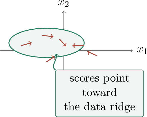
5.0.10.2 Forward and Reverse SDEs
A common continuous-time noising process is the variance-preserving SDE \[\require{physics} \dd X_t = f(X_t,t)\,\dd t+g(t)\,\dd W_t, \qquad X_0\sim p_{\mathrm{data}}.\] The drift \(f\) contracts or rescales the signal, and the diffusion coefficient \(g\) controls how much Brownian noise is injected. The discrete DDPM forward chain can be viewed as an Euler discretization of this idea. Score-based SDE models make this continuous-time interpretation explicit [52].
Theorem 0.57 (Reverse-time SDE, informal). Under suitable smoothness and nondegeneracy assumptions, if the forward SDE has marginal density \(p_t\), then the reverse-time dynamics are \[\require{physics} \dd X_t = \bigl[f(X_t,t)-g(t)^2\nabla_x\log p_t(X_t)\bigr]\,\dd t +g(t)\,\dd \bar W_t,\] where time is run from \(T\) back to \(0\) and \(\bar W_t\) denotes reverse-time Brownian motion.
The theorem identifies the only unknown term in reverse sampling: the score \(\nabla_x\log p_t\). Replacing it by a neural score estimate \(s_\theta(x,t)\) gives a practical sampler.
The sign and time orientation are easy to confuse. The displayed equation is written for the reverse-time process: the sampler starts at a large time \(T\), where \(p_T\) is close to a simple Gaussian, and integrates back toward time zero. The score term corrects the Brownian dynamics so that the marginal laws move from noisy distributions back toward the data distribution.
5.0.10.3 Probability-Flow ODE
The same marginal path can also be generated by a deterministic ODE.
The probability-flow ODE \[\require{physics} \frac{\dd X_t}{\dd t} = f(X_t,t)-\frac{1}{2}g(t)^2\nabla_x\log p_t(X_t)\] has the same one-time marginals \(p_t\) as the forward SDE.
This proposition is one of the central bridges between diffusion and deterministic transport. It enables likelihood computation through a continuous normalizing flow and connects score-based models to ODE solvers.
The factor \(1/2\) in the ODE is not arbitrary. At the density level, the diffusion term in the Fokker–Planck equation can be rewritten using \(\Delta p_t=\operatorname{div}(p_t\nabla\log p_t)\). Moving half of this score-induced flux into the deterministic velocity gives a continuity equation with the same marginal evolution. The resulting ODE and SDE do not generate the same random paths, but they agree on the distribution at each time.

The density dynamics make this equivalence precise. The SDE marginal density satisfies the Fokker–Planck equation \[\partial_t p_t = -\operatorname{div}(f p_t) + \frac{1}{2}g(t)^2\Delta p_t.\] By contrast, an ODE with velocity \(v_t\) satisfies the continuity equation \[\partial_t p_t=-\operatorname{div}(v_t p_t).\] For diffusion, the probability-flow velocity is \[v_t=f-\frac{1}{2}g(t)^2\nabla_x\log p_t.\]
The sampler design space is therefore broad. Stochastic samplers are often robust and explore noisy paths. ODE samplers are deterministic and can be faster. Distillation and rectification seek to reduce the number of function evaluations while preserving the learned transport.
This distinction also clarifies evaluation. If the learned score were exact and the numerical solver exact, both the reverse SDE and the probability-flow ODE would reproduce the desired marginal path. In practice, however, neural approximation error and discretization error interact differently with stochastic and deterministic samplers. Choosing a sampler is therefore part of the modeling problem, not merely an implementation detail.
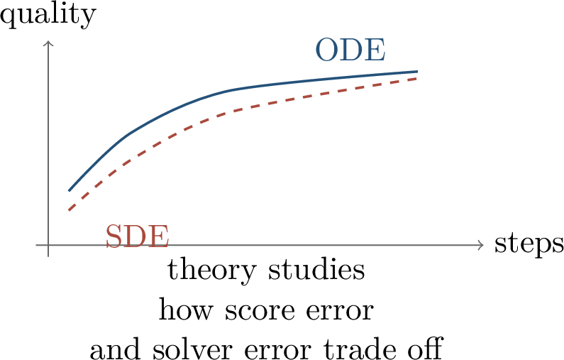
5.0.11 Learning Scores↩︎
5.0.11.1 Denoising Score Matching
The basic identity behind diffusion training says that Gaussian denoising recovers the score of the corrupted distribution.
Lemma 0.25 (Gaussian corruption score). Let \[X_t=\alpha_t X_0+\sigma_t\varepsilon, \qquad \varepsilon\sim\mathcal{N}(0,I),\] and let \(p_t\) be the density of \(X_t\). Then \[\nabla_x\log p_t(x) = \E\!\left[ -\frac{x-\alpha_tX_0}{\sigma_t^2} \,\middle|\, X_t=x \right].\]
Proof. Write \(q_t(x\mid x_0)\) for the Gaussian conditional density of \(X_t\) given \(X_0=x_0\). Its score is explicit: \[\nabla_x\log q_t(x\mid x_0) = -\frac{x-\alpha_t x_0}{\sigma_t^2}.\] Since \(\require{physics} p_t(x)=\int q_t(x\mid x_0)p_{\mathrm{data}}(x_0)\,\dd x_0\), differentiating under the integral gives \[\require{physics} \nabla p_t(x) = \int q_t(x\mid x_0) \nabla_x\log q_t(x\mid x_0)p_{\mathrm{data}}(x_0)\,\dd x_0.\] Dividing by \(p_t(x)\) turns the right-hand side into the conditional expectation given \(X_t=x\). ◻
Thus denoising is not merely a heuristic. It estimates a conditional average of exact local likelihood gradients. The equivalent small-scale identity \[\E[\varepsilon\mid X_t=x] = -\sigma_t\nabla_x\log p_t(x)\] follows by substituting \(x-\alpha_tX_0=\sigma_t\varepsilon\).
The lemma also explains why different DDPM parameterizations are mathematically interchangeable in the idealized population setting. Predicting the clean signal \(x_0\), predicting the added noise \(\varepsilon\), and predicting the score all determine one another through known affine transformations and conditional expectations. In finite neural networks they may behave differently numerically, but they are tied to the same denoising identity.
5.0.11.2 Vector-Field Regression
A standard score matching loss is \[\min_\theta \E_{t,x_t} \lambda(t) \left\lVert s_\theta(x_t,t)-\nabla_x\log p_t(x_t) \right\rVert^2.\] In practice the unknown true score is replaced by the denoising target supplied by the previous lemma. The weight \(\lambda(t)\) balances noise levels. The mathematical burden is that accuracy must hold along the entire sampling path, not merely near the original data manifold.
The weighting \(\lambda(t)\) is a modeling choice with statistical consequences. Small noise levels carry fine data geometry but can have large, rapidly varying scores. Large noise levels are smoother but contain less information about individual data samples. A training objective that overemphasizes one region of time may produce a field that works well there and poorly elsewhere; the sampler, however, must traverse all relevant times.
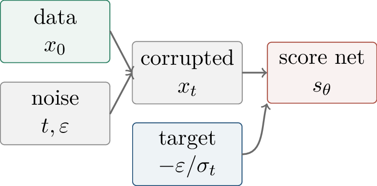
Several sources of error must be controlled to turn score learning into a guarantee for generated samples. The learned score may differ from the true score, the numerical solver introduces time-discretization error, and the initialization or terminal truncation may leave tail error.
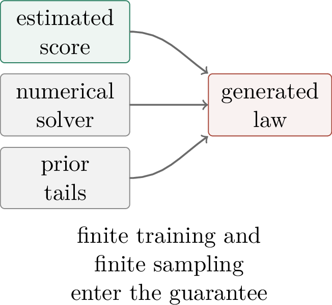
Theorem 0.58 (Informal error decomposition). Assume the target density is regular, the score estimator satisfies \[\require{physics} \int_0^T \E_{p_t}\left\lVert s_\theta(X_t,t)-s_t(X_t) \right\rVert^2\,\dd t \le \varepsilon_{\mathrm{score}}^2,\] and the sampler has step size \(h\). Many analyses prove bounds of the form \[\begin{align} \mathrm{dist}(p_{\theta,0},p_{\mathrm{data}}) &\le C\bigl( \varepsilon_{\mathrm{score}} +\varepsilon_{\mathrm{disc}}(h) +\varepsilon_{\mathrm{tail}} \bigr), \end{align}\] where the distance may be KL divergence, total variation, or a Wasserstein metric, and the constant \(C\) depends on smoothness, tails, time horizon, and dimension.
This informal statement is deliberately schematic. Different papers impose different assumptions and prove different metrics, but the structure is stable: field error enters through the learned score or velocity, discretization error enters through the numerical integrator, and tail or initialization error enters because the sampler starts from an approximate terminal distribution. The exponential dependence on a Lipschitz or stability constant is also typical of ODE/SDE perturbation arguments.
Low-density regions can have large or unstable scores; vector-field regression in high dimension needs structural assumptions; and the sampler visits points drawn from its own approximate law. Diffusion works in practice because the noising path creates smooth intermediate distributions, but a proof must control all of them.
Example 0.14 (A one-dimensional Gaussian score). If \(X_t\sim \mathcal{N}(0,\sigma_t^2)\) on \(\R\), then \[\nabla_x\log p_t(x)=-\frac{x}{\sigma_t^2}.\] The score points back toward the mean, and its magnitude grows linearly with \(|x|\). In high-dimensional diffusion models the same local idea remains: the score field points toward regions of larger corrupted-data density, but the geometry of those regions is learned from data rather than given by a single Gaussian formula.
5.0.12 Flow Matching↩︎
5.0.12.1 The Continuity Equation
Flow matching starts from the deterministic transport equation rather than from a stochastic noising process.
Definition 0.82 (Velocity field). A time-dependent velocity \(v_t:\R^d\to\R^d\) transports densities through the continuity equation \[\partial_t p_t(x)+\operatorname{div}\!\bigl(p_t(x)v_t(x)\bigr)=0.\] If \(X_t\) follows \(\dot{X}_t=v_t(X_t)\), then \(X_t\sim p_t\) whenever the initial law is \(p_0\).
Normalizing flows learn an invertible map, while flow matching learns the velocity of the map directly. The central design choice is the path of probability measures \(p_t\) joining \(p_{\mathrm{base}}\) to \(p_{\mathrm{data}}\). The modern flow-matching formulation of Lipman et al. [53] shows that one can train this velocity by supervised regression against known conditional velocity labels.
5.0.12.2 Conditional Paths
Sample \(z\sim p_{\mathrm{base}}\) and \(x\sim p_{\mathrm{data}}\). A simple conditional path is the linear interpolation \[X_t=(1-t)z+t x, \qquad u_t=x-z.\] More general paths may use time-dependent means and variances. The key advantage is that the conditional velocity \(u_t\) is known, so the training target is again supervised.
This is the analogue of the denoising trick in diffusion. We do not know the marginal velocity field \(v_t(x)\) directly, because many conditional paths may pass through the same point \(x\) at time \(t\). But we can sample a pair \((z,x)\), construct a point on its conditional path, and write down the velocity of that path. Squared loss then projects these conditional velocities onto a function of the observed state \(X_t\).
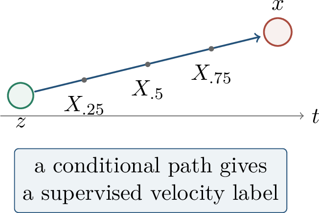
The flow matching objective is \[\min_\theta \E_{t,z,x} \left\lVert v_\theta(X_t,t)-u_t(X_t\mid z,x) \right\rVert^2.\] The notation \(u_t(X_t\mid z,x)\) emphasizes that the target is the velocity of the conditional path associated with the sampled pair.
For the squared loss above, the population minimizer satisfies \[v_t^\star(y) = \E[u_t(X_t\mid z,x)\mid X_t=y],\] and this conditional expectation is the marginal velocity transporting the marginal density \(p_t\).
Proof. For each \(t\), squared loss over functions of \(X_t\) is minimized by the orthogonal projection of the target \(u_t\) onto the sigma-field generated by \(X_t\). Hence \[\argmin_v \E\left\lVert v(X_t,t)-u_t \right\rVert^2 = \E[u_t\mid X_t,t].\] Marginalizing the conditional continuity equations over the sampled pairs shows that this projected velocity solves the continuity equation for the marginal path \(p_t\). ◻
This proof is short but conceptually important. Conditional flow matching does not require the neural network to know which pair \((z,x)\) produced the point \(X_t=y\). It only observes \(y\) and \(t\). Therefore the best possible network output is the average conditional velocity among all sampled paths that pass through \(y\) at time \(t\). That average is exactly the marginal velocity needed by the continuity equation.
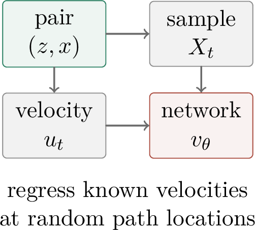
5.0.12.3 Rectification and Couplings
The simplest independent coupling between \(z\) and \(x\) may create curved or crossing marginal trajectories. Rectified flow trains on interpolated pairs, then re-samples pairs from the learned flow and trains again. The goal is to straighten paths so that fewer ODE solver steps are needed.
Path straightness matters because numerical integration pays for curvature. If trajectories bend sharply, a coarse solver can drift away from the intended transport. If trajectories are nearly straight and the velocity varies slowly, larger solver steps may suffice. Rectification should therefore be understood as a joint statistical and numerical strategy: it changes the regression problem in order to make sampling cheaper.

Coupling matters. If base and data samples are paired independently, the conditional paths can cross in complicated ways. Minibatch optimal-transport couplings match base samples to data samples so as to reduce path length or crossing. This changes the regression distribution and can make the learned velocity field smoother.
The coupling is not identifiable from the marginals alone. Many joint laws can have the same base and data marginals, but they induce different conditional paths and different regression targets. A good coupling pairs points so that the resulting velocity field is simple; a bad coupling can force the network to average incompatible directions at the same location.
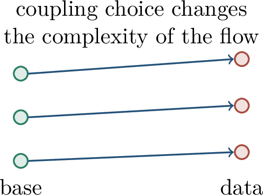
5.0.13 Unification and Solvers↩︎
5.0.13.1 Two Views of the Same Transport Problem
Diffusion and flow matching can be placed side by side: \[\text{diffusion/score:}\qquad \text{learn }s_t(x)=\nabla\log p_t(x), \qquad v_t(x)=f(x,t)-\frac{1}{2}g(t)^2s_t(x),\] where the path is induced by a noising SDE. Flow matching instead chooses a path \(X_t\) and learns \[\text{flow matching:}\qquad v_t(x)=\E[u_t\mid X_t=x]\] directly. Both views learn local fields along a path; they differ in how the path is specified and which supervised label is used.
This comparison helps organize the terminology. A score model first learns \(\nabla\log p_t\) and then converts it into a reverse SDE or probability-flow velocity. A flow-matching model learns the velocity itself. A stochastic interpolant sits between the two: it specifies an interpolation with optional noise and can lead to either score-like or velocity-like training targets.
Stochastic interpolants provide a flexible template: \[X_t=I_t(X_0,X_1)+\gamma_t Z, \qquad Z\sim\mathcal{N}(0,I).\] Here \(I_t\) interpolates between base and data, while \(\gamma_t\) adds noise. When \(\gamma_t=0\), we recover deterministic flow matching; when \(\gamma_t>0\), the path becomes diffusion-like.
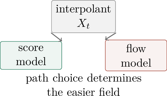
5.0.13.2 Solver and Neural Error
Given a learned field \(v_\theta\), ODE sampling solves \[\dot{X}_t=v_\theta(X_t,t), \qquad X_0\sim p_{\mathrm{base}}.\] If the true field is Lipschitz with constant \(L\), a typical trajectory error bound has the schematic form \[\require{physics} \sup_t\left\lVert X_t-\widehat X_t \right\rVert \lesssim e^{LT} \left( \int_0^T \left\lVert v_t-v_{\theta,t} \right\rVert\,\dd t + \text{solver error} \right).\] This expression makes a recurring theme explicit: training error and numerical error interact. A field that is easier to approximate may not be the field that admits the shortest solver trajectory, and vice versa.
The stability factor \(e^{LT}\) is a warning. Even small local vector-field errors can be amplified by an unstable flow. This is one reason path design is not cosmetic: smoother and less expansive fields can improve both learning and sampling error. Conversely, aggressive few-step samplers may demand a more accurate or more stable learned field.
5.0.13.3 Guidance
Conditional generation often uses guidance. In classifier-free guidance, a conditional and an unconditional prediction are combined at the same noisy input and time: \[\begin{align} s_{\mathrm{guid}} &= s_{\mathrm{uncond}}+w\,\Delta s,\\ \Delta s &= s_{\mathrm{cond}}-s_{\mathrm{uncond}}. \end{align}\] Increasing \(w\) usually improves condition fidelity but reduces diversity. For flow models, analogous guidance modifies velocities rather than scores.
Guidance is best viewed as a controlled distortion of the learned transport. The unconditional field describes how to sample from the broad data distribution, while the conditional correction pushes samples toward a desired class or text condition. Large guidance weights can make the conditional signal visually strong, but they also move the sampler away from the distribution on which the field was trained. This explains the common fidelity-diversity tradeoff.
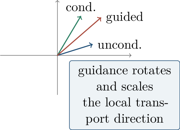
5.0.13.4 When Is Flow Matching Easier?
A path is easy when its marginal velocity field is smooth, low-curvature, and aligned with the data geometry. Independent linear interpolation is simple but can create crossing trajectories. Optimal-transport couplings can reduce kinetic energy. Diffusion paths smooth the data, which can improve score estimation. The open tension is that the easiest path for optimization may not be the shortest path for sampling.
There is no universally best path. A path with heavy noise may make the learning problem smoother but require many denoising steps. A nearly deterministic straight path may allow fast ODE sampling but create sharp velocity discontinuities if the coupling is poor. Modern generative modeling therefore treats path design, coupling design, neural approximation, and solver choice as one coupled problem.
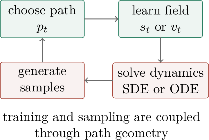
5.0.14 Limitations, Connections, and Outlook↩︎
5.0.14.1 What Current Theory Explains
Current theory explains several important pieces. Denoising losses identify scores or velocities under ideal sampling. Continuous-time samplers have clean PDE interpretations through the Fokker–Planck and continuity equations. Error bounds decompose generated-distribution error into score or velocity estimation, solver discretization, and tail terms.
These explanations are already substantial. They show why a supervised loss on corrupted examples can train an unsupervised generator, why stochastic and deterministic samplers can share the same marginal path, and why local field accuracy is the central statistical object. They also clarify how diffusion and flow matching fit into a common language of transporting probability measures.
The hard parts are also clear. Realistic image models use structured architectures and finite data. Guidance, conditioning, and text-image alignment are still under-theorized. Fast few-step generation changes the approximation problem because the model must represent a much more aggressive transport map.
The gap between theory and practice is therefore not a single missing lemma. It includes finite-sample learning of high-dimensional vector fields, the interaction between learned neural fields and numerical solvers, the effect of conditioning and guidance, and the role of architecture. A useful theory must eventually connect all four.
5.0.14.2 Connections to Earlier Chapters
| Earlier topic | Connection to diffusion and flows |
|---|---|
| Approximation | neural networks represent score and velocity fields |
| Optimization | denoising and flow matching are supervised regression over noise levels or path times |
| Generalization | vector-field error controls distributional error through sampler stability |
| Robustness | score fields can be sensitive off the data manifold |
| GANs | diffusion replaces a discriminator by a path-based objective |
| Transformers | modern generators often use transformer backbones |
Example 0.15 (Noise prediction equals score prediction). Let \(X_0\sim p_{\mathrm{data}}\), \(X_t=\alpha_tX_0+\sigma_t\varepsilon\), and \(\varepsilon\sim\mathcal{N}(0,I)\). The Gaussian corruption identity gives \[\E[\varepsilon\mid X_t=x] = -\sigma_t\nabla_x\log p_t(x).\] Therefore predicting Gaussian noise and predicting the score are equivalent up to a known scale. This is the simplest calculation behind the DDPM parameterization.
DDPMs and score-SDE models learn a family of denoising vector fields along a noising path. Flow matching learns a transport velocity directly from conditional paths. The central mathematical objects are scores, continuity equations, couplings, and finite-error propagation.
Chapter Synthesis
Diffusion models and flow matching learn local fields along paths from a simple base law to the data law.
DDPMs use a fixed Gaussian noising chain and train a neural network by supervised denoising regression.
Gaussian denoising identifies the score of the corrupted distribution, linking noise prediction and score prediction.
Score-based SDEs, reverse-time SDEs, and probability-flow ODEs describe stochastic and deterministic samplers with related marginal laws.
Flow matching chooses conditional paths and regresses known velocity labels; the conditional expectation of those labels gives the marginal velocity.
Sampling quality depends jointly on field estimation, path geometry, coupling design, guidance, and numerical solver error.
Foundational references include Sohl-Dickstein et al., Deep Unsupervised Learning using Nonequilibrium Thermodynamics, Song and Ermon, Generative Modeling by Estimating Gradients of the Data Distribution, Ho, Jain, and Abbeel, Denoising Diffusion Probabilistic Models [20], Song, Meng, and Ermon, Denoising Diffusion Implicit Models, Song et al., Score-Based Generative Modeling through Stochastic Differential Equations [52], and Karras et al., Elucidating the Design Space of Diffusion-Based Generative Models. For flow matching and unified transport views, see Lipman et al., Flow Matching for Generative Modeling [53], Liu, Gong, and Liu, Flow Straight and Fast, Tong et al., Improving and Generalizing Flow-Based Generative Models with Minibatch Optimal Transport, Albergo, Boffi, and Vanden-Eijnden, Stochastic Interpolants, and Pooladian et al., Multisample Flow Matching. Error analyses for flow matching include Pooladian et al., Error Bounds for Flow Matching Methods.
The natural next questions concern fast sampling and generative transformers. Distillation, consistency models, and one-step generators ask how much of the transport can be compressed into very few evaluations. Transformer backbones raise a complementary representation question: how do attention-based networks implement denoising or velocity fields at scale? Diffusion and flow matching therefore turn generative modeling into the study of learned transport under finite data, finite compute, and finite solver accuracy.
5.0.15 Why Scaling Laws?↩︎
Modern deep learning is shaped by the fact that validation loss often changes predictably as model size, data, and compute grow. These empirical regularities are not merely descriptive curves. They are planning tools: before spending a large budget, one can run smaller experiments, fit a law, and use it to choose how to allocate resources.
The word “law” should be read with care. Scaling laws are empirical regularities measured over a controlled experimental family, not universal physical laws. They become useful when the model architecture, data mixture, optimizer, tokenizer, and evaluation protocol remain comparable across runs. Within such a regime, a fitted curve can be a remarkably effective engineering instrument: it converts expensive design choices into quantitative forecasts.
The guiding question of this chapter is:
How should one split a fixed budget between training a stronger base model and spending more computation at test time?
Classical scaling laws answer the first half of this question by studying pretraining loss as a function of parameters \(N\), tokens \(D\), and training compute. Newer inference-scaling work asks when repeated samples, longer reasoning, search, or verification can improve deployed performance more cheaply than increasing the base model.
The second half is becoming increasingly important because deployment is often query-specific. Training a larger base model improves all future queries but requires a large up-front cost. Spending more compute at inference improves only the current query, but it can be targeted: easy queries can be answered quickly, while hard or high-value queries can receive more deliberation. The right allocation therefore depends on the expected number of future queries, latency constraints, and whether there is a reliable way to recognize a better answer.

Definition 0.83 (Training-time and test-time scaling). Training-time scaling chooses \(N\) and \(D\) under a training compute budget \[C_{\mathrm{train}}\approx \kappa ND,\] where \(\kappa\) depends on the architecture and implementation. Test-time scaling uses extra computation after training to answer a particular query: multiple samples, longer deliberation, search over partial solutions, verification, or reranking. Its cost \(C_{\mathrm{infer}}\) is roughly the number of model calls times the number of generated or scored tokens per call.
The unifying view is simple: scaling laws model error as a function of resources. The difficulty is that the relevant resource is no longer only a pretraining budget. It may also include the number of candidate solutions, the depth of a search tree, the cost of a verifier, latency constraints, and the task distribution.
This chapter treats scaling as a resource-allocation problem rather than only as a curve-fitting problem. A fitted exponent tells us the marginal return of one resource in a specified regime. A deployment decision compares marginal returns across resources: more parameters, more data, more samples, more search depth, or a better verifier.
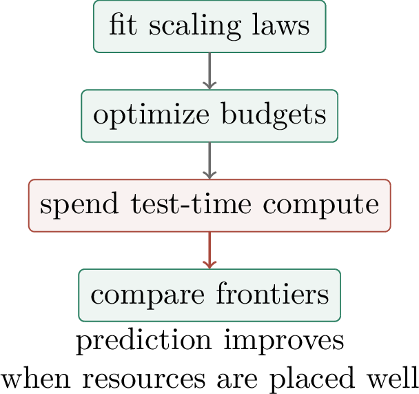
5.0.16 Empirical Scaling Laws↩︎
5.0.16.1 Power-Law Loss Curves
Definition 0.84 (Scaling law). A basic scaling law models population or validation loss as \[L(C)=L_{\infty}+ A C^{-\alpha}, \qquad A,\alpha>0.\] Here \(C\) may denote model size, data, or compute. The constant \(L_{\infty}\) is an asymptotic loss floor, and \(\alpha\) is the return-to-scale exponent.
Power-law scaling for language models was studied systematically by Kaplan et al. [21]. The basic empirical observation is that, over large but finite regimes, excess loss often decays approximately linearly on a log-log plot. The exponent \(\alpha\) is small in many language-model experiments, which means that large multiplicative increases in compute can produce only modest additive reductions in loss. This is why accurate budget allocation matters.
Subtracting the floor gives \[\log(L(C)-L_{\infty})=\log A-\alpha\log C.\] Thus a power law appears nearly linear on log-log axes. The slope is the negative exponent. Different experimental regimes can have different slopes, which is why the law must be treated as a local empirical model rather than as a universal theorem.
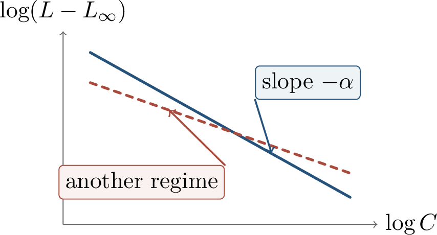
For language models, a common separable approximation is \[L(N,D) = L_{\infty}+ A N^{-\alpha}+B D^{-\beta}.\] The first term after the floor represents capacity or approximation error; the second represents data-limited estimation error. In practice this formula is an approximation to a smooth region of an empirical frontier. It is useful when it predicts held-out larger experiments and its residuals remain structured.
The separable form is also pedagogically useful because it exposes two failure modes. If \(N\) is too small relative to \(D\), the model is capacity-limited: more data mostly repeats a lesson the model cannot fully represent. If \(D\) is too small relative to \(N\), the model is data-limited: additional parameters are undertrained. Compute-optimal scaling tries to stay near the boundary where neither bottleneck is overwhelmingly dominant.
5.0.16.2 Fitting and Stress-Testing
Suppose we run many smaller experiments and observe losses \(L_i\) at \((N_i,D_i)\). A scaling model may be fitted by nonlinear least squares: \[\begin{align} \widehat L(N,D) &= L_{\infty}+ A N^{-\alpha}+B D^{-\beta},\\ \theta_{\mathrm{law}} &= \argmin_\theta \sum_i\bigl(L_i-\widehat L(N_i,D_i)\bigr)^2. \end{align}\] The fitted \(L_{\infty}\) requires care: an error in the floor can distort exponent estimates. Extrapolation should be tested by holding out some budgets or by checking a larger run after fitting on smaller ones.
In practice one should inspect residuals, not only the fitted exponent. If the residuals are systematic rather than noise-like, the model may be missing a regime change, a data-mixture effect, or an optimization artifact. A useful scaling law is not the one with the most elegant formula; it is the one that predicts held-out runs at the scale where decisions will actually be made.
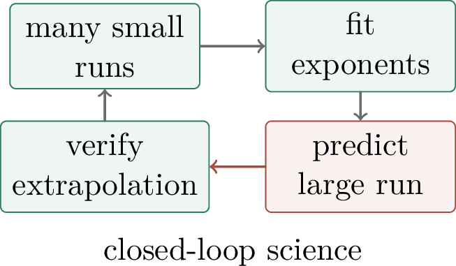
A fitted power law summarizes a regime; it does not identify the mechanism by itself. Dataset mixture, tokenizer, optimizer, architecture, and evaluation all matter. Scaling can break near contamination, saturation, distribution shift, or qualitative changes in model behavior.
This remark is especially important for benchmark interpretation. A loss curve can be smooth while a thresholded metric changes abruptly, and a multiple-choice benchmark can saturate even when the underlying distributional loss still improves. Conversely, an apparent jump in a metric may reflect the metric transformation rather than a sudden new capability. Later chapters on emergence return to this distinction.
5.0.17 Compute-Optimal Training↩︎
5.0.17.1 The Training Budget
For a dense Transformer trained on \(D\) tokens with \(N\) non-embedding parameters, a rough compute model is \[C_{\mathrm{train}}\approx \kappa ND.\] Increasing \(N\) reduces capacity error; increasing \(D\) reduces data-limited error. Compute-optimal training asks how to choose the pair \((N,D)\) on a fixed compute contour.
The approximation \(C_{\mathrm{train}}\approx \kappa ND\) suppresses constants and architecture details, but it captures the dominant tradeoff for dense autoregressive Transformers. Each token update uses the model parameters, and training over more tokens repeats that computation. Thus model size and token count are not independent luxuries; they compete for the same training budget.
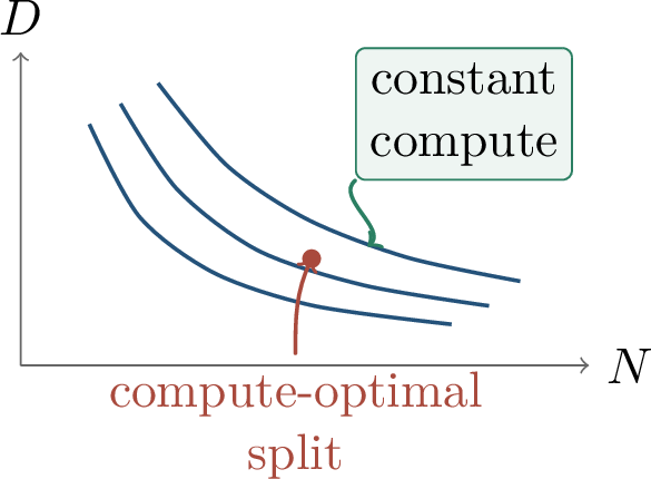
Assume \[L(N,D)-L_{\infty}= A N^{-\alpha}+B D^{-\beta}, \qquad ND=C.\] Then the compute-optimal allocation obeys \[N_\star\propto C^{\beta/(\alpha+\beta)}, \qquad D_\star\propto C^{\alpha/(\alpha+\beta)}.\] The constants \(A\) and \(B\) determine the exact ratio at a given scale.
Proof. Substitute \(D=C/N\). The excess loss becomes \[A N^{-\alpha}+B C^{-\beta}N^\beta.\] At an interior optimum, \[\alpha A N^{-\alpha-1} = \beta B C^{-\beta}N^{\beta-1}.\] Rearranging gives \(N^{\alpha+\beta}\asymp C^\beta\), hence \(N_\star\propto C^{\beta/(\alpha+\beta)}\). Since \(D_\star=C/N_\star\), the token count scales as \(D_\star\propto C^{\alpha/(\alpha+\beta)}\). ◻
The proof expresses a marginal-return condition. If model error dominates, one should grow \(N\); if data error dominates, one should train longer. At the optimum, the marginal return from extra model size is balanced with the marginal return from extra data.
The exponent formula has a simple interpretation. The resource whose error term decays more slowly receives more of the compute growth. In the example where \(\beta<\alpha\), the data-limited term \(D^{-\beta}\) improves slowly, so the optimal allocation grows \(D\) faster than \(N\). This is not a moral preference for data over parameters; it is the consequence of the fitted returns in the assumed regime.
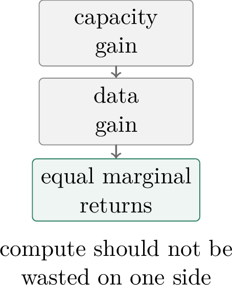
5.0.17.2 Kaplan, Chinchilla, and Data Constraints
Early language-model scaling estimates favored very large models trained on comparatively fewer tokens. The Chinchilla analysis found that many large models were undertrained: at the same compute, smaller models trained on many more tokens achieved lower loss. The important point is not a single preferred model size, but a frontier: the optimal pair \((N,D)\) changes with compute and with the fitted exponents.
This historical shift is usually summarized as a move from parameter-heavy training toward more data-balanced training. Hoffmann et al. [54] showed empirically that, for their training setup, compute-optimal language models should use substantially more tokens per parameter than many earlier large-model runs. The lesson for theory is that the optimum is not determined by \(C\) alone; it is determined by the entire experimental regime used to fit the law.
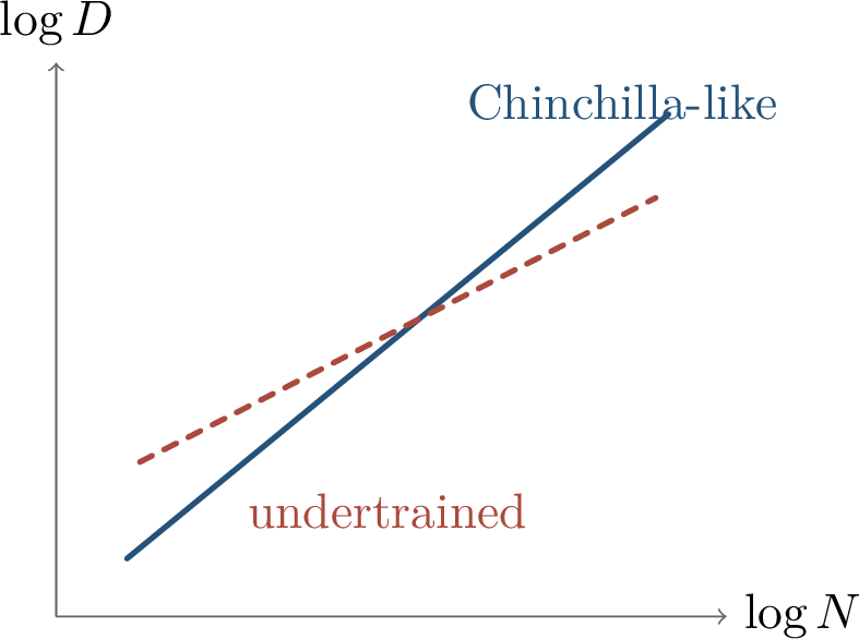
High-quality data may be finite. If \(D\) must exceed unique data, training repeats examples. Repetition can still help, but marginal returns often degrade. Synthetic data, filtering, curriculum, and mixture design change the effective token count, so data-constrained scaling is about quality and diversity as much as raw token number.
It is therefore useful to distinguish raw tokens from effective information. Two corpora with the same number of tokens can have different coverage, duplication, difficulty, contamination, and relevance to downstream tasks. Repeated tokens may still improve optimization and memorization of rare facts, but they are not equivalent to fresh independent samples. Synthetic data can increase coverage or impose structure, but it can also amplify model biases if generated and filtered poorly.
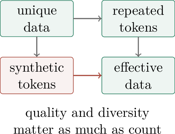
5.0.18 Mechanisms Behind Power Laws↩︎
5.0.18.1 Spectral Tails and Effective Dimension
One possible mechanism is spectral. Suppose a target function has energy spread over many modes, and training learns modes in decreasing signal-to-noise order. Smooth spectra often have algebraic tails; more data or parameters reveal more modes; and the observed exponent reflects both data geometry and model bias.
This mechanism is intentionally abstract. It does not claim that a language model literally diagonalizes a fixed kernel and learns one eigenfunction at a time. Rather, it gives a mathematical toy model for why scale-free curves can appear. If the problem contains many directions of decreasing importance, and additional resources steadily unlock lower-energy directions, then the remaining unexplained energy can decay like a power law.
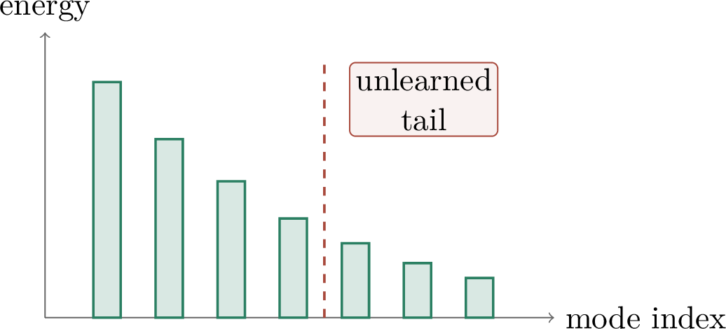
This picture connects scaling laws to the themes of previous chapters. A useful mental decomposition is \[L-L_{\infty} \approx \underbrace{\text{approximation}}_{N} + \underbrace{\text{estimation}}_{D} + \underbrace{\text{optimization}}_{\text{training recipe}}.\] Approximation improves when the hypothesis class expands. Estimation improves when more independent information arrives. Optimization determines which part of the class is reachable by the actual training procedure.
These three terms are not directly observable from a single validation curve. A larger model may improve approximation but worsen optimization if the training recipe is not adjusted. More data may improve estimation but change the data distribution if the additional tokens are lower quality. A new optimizer may improve the reachable frontier without changing the nominal \((N,D)\) budget. Scaling-law interpretation is therefore always conditional on the experimental protocol.
Definition 0.85 (Effective dimension). For feature or kernel eigenvalues \(\lambda_j\), the scale-dependent effective dimension at regularization level \(\mu>0\) is \[d_{\mathrm{eff}}(\mu) = \sum_j \frac{\lambda_j}{\lambda_j+\mu}.\] If the eigenvalues decay polynomially, \(d_{\mathrm{eff}}(\mu)\) grows polynomially as \(\mu\) decreases, which can lead to power-law learning curves.
The quantity \(d_{\mathrm{eff}}(\mu)\) softly counts directions with eigenvalues above the scale \(\mu\). If \(\lambda_j\gg\mu\), the corresponding term contributes nearly one; if \(\lambda_j\ll\mu\), it contributes little. Lowering \(\mu\) is analogous to resolving finer and lower-variance directions of the problem. Polynomial eigenvalue tails then translate resolution into power-law growth of effective dimension.
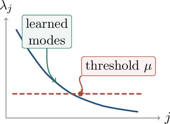
Suppose the remaining target energy after learning \(m\) modes satisfies \[\sum_{j>m}a_j^2\le C_0 m^{-r}.\] If the number of reliably learned modes grows as \(m(n)\asymp n^\gamma\), then \[L(n)-L_{\infty}\lesssim n^{-r\gamma}.\]
Proof. After \(n\) samples or units of resource, assume the algorithm reliably learns the first \(m(n)\) modes. The remaining error is bounded by the spectral tail, so \[L(n)-L_{\infty} \lesssim m(n)^{-r} \asymp (n^\gamma)^{-r} = n^{-r\gamma}.\] ◻
The proposition is a mechanism, not a universal theorem for language models. It explains why an exponent can encode both the geometry of the data and the efficiency of the algorithm. Prediction remains hard because the experimental family can drift: the data mixture changes, the optimizer or architecture changes, a benchmark saturates, or the model develops qualitatively new multi-step behavior.
This is also why extrapolation should be local. A fitted line on a log-log plot can remain accurate across several orders of magnitude and then fail when a new bottleneck appears. Examples include running out of high-quality data, changing context length, entering a memory-bandwidth-limited hardware regime, or evaluating on a benchmark that rewards a qualitatively different behavior.
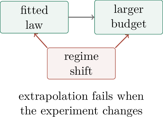
5.0.19 Test-Time Compute↩︎
5.0.19.1 Sampling, Checking, and Deliberation
Definition 0.86 (Test-time compute). Test-time compute is extra computation used after the model is trained to answer a specific query. Examples include sampling several candidate solutions, generating longer chains of thought, searching over partial solutions, and verifying or reranking candidates.
The phrase covers several different mechanisms. Repeated sampling uses parallel attempts. Deliberation uses longer trajectories for one attempt. Search uses branching and pruning over partial states. Verification spends compute to evaluate or rank candidate answers. These mechanisms can be combined, but their scaling behavior can be very different.
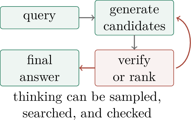
Lemma 0.26 (Oracle pass probability). If each independent sample solves a problem with probability \(p\), then the probability that at least one of \(K\) samples is correct is \[P_{\mathrm{pass}}(K)=1-(1-p)^K.\]
Proof. The probability that no sample is correct is \((1-p)^K\). Taking the complement gives the formula. ◻
The failure probability is therefore \[1-P_{\mathrm{pass}}(K)=(1-p)^K.\] This is a simple scaling law for repeated sampling: failure decays exponentially in \(K\) under independence and oracle selection. In real systems, samples are correlated and verifiers are imperfect, so the curve is often shallower.
The independence and oracle-selection assumptions are doing nearly all the work. If all samples make the same mistake, increasing \(K\) does not help. If a correct answer appears but the system cannot identify it, the pass probability over candidates may improve while the final answer does not. Repeated sampling is therefore most valuable when candidate diversity and selection quality grow together.
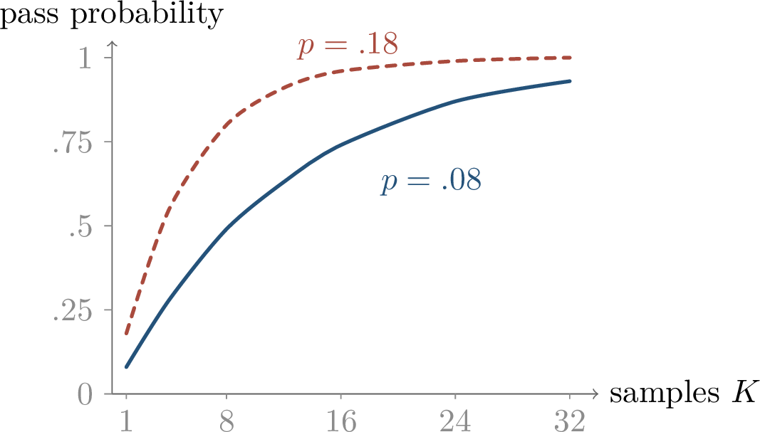
5.0.19.2 Self-Consistency and Verifiers
Self-consistency samples multiple reasoning traces and aggregates their final answers by majority vote or confidence. The method is useful when the model can find diverse paths to the same correct answer and when errors are not perfectly correlated. It can fail if many samples share the same misconception.
Self-consistency is a weak verifier built from the model’s own distribution. It assumes that correct reasoning paths are more stable across samples than incorrect paths. This can be true for arithmetic or symbolic problems where several derivations converge to the same answer. It is less reliable when the model has a systematic bias, because repeated traces can reinforce the same false conclusion.
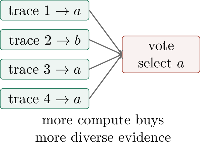
Let \(Y_1,\ldots,Y_K\) be candidate answers with verifier scores \(R(Y_i)\). A verifier-guided best-of-\(K\) policy outputs \[\widehat Y=\argmax_{1\le i\le K} R(Y_i).\] Improvement from extra samples requires the verifier ranking to correlate with correctness.
Outcome reward models score final answers, while process reward models score intermediate reasoning steps. A strong verifier can turn sampling into a search procedure. A weak verifier can do the opposite: it may select a confidently wrong answer from a larger set.
The distinction between generation and verification is central. Some tasks are hard to solve but easy to check, such as many mathematical or programming problems with deterministic tests. Other tasks, such as open-ended writing or ambiguous advice, have no cheap objective verifier. Test-time compute scales best in the first regime because the system can convert many imperfect attempts into one checked solution.
5.0.19.3 Search Over Thoughts
Instead of sampling full solutions independently, one can spend compute on a tree of partial solutions. Branching expands alternatives, evaluation prunes poor states, and depth supports multi-step planning. This is especially useful when intermediate states are meaningful and can be evaluated.
Tree search also introduces a new allocation problem inside inference. With a fixed budget, one can increase breadth, depth, or evaluation accuracy. More breadth explores diverse possibilities; more depth pursues longer chains of reasoning; better evaluation reduces the chance of pruning a promising branch. The best tradeoff depends on the task’s branching factor and on how informative partial-state evaluations are.
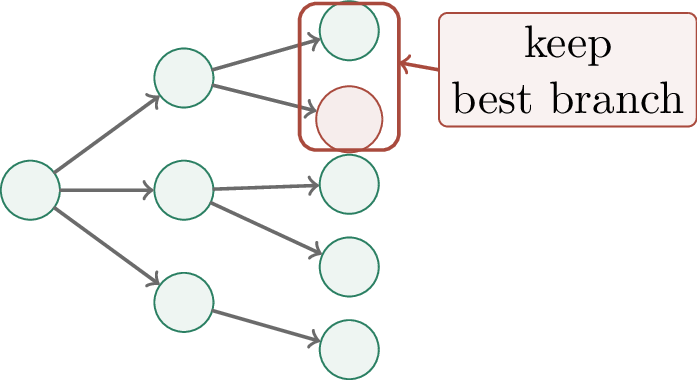
5.0.20 Joint Scaling of Training and Inference↩︎
5.0.20.1 An Inference-Aware Objective
For a trained model and a test-time policy \(\pi\), write the deployment loss as \[L_{\mathrm{deploy}} = L(N,D,\pi;C_{\mathrm{train}},C_{\mathrm{infer}}), \qquad C_{\mathrm{total}}=C_{\mathrm{train}}+C_{\mathrm{infer}}.\] Training compute buys a stronger base policy for all future queries. Inference compute buys more search, sampling, and verification for each query. The optimal split depends on the task distribution, latency, amortization across queries, and whether answers can be checked.
The amortization point is crucial. If a model will answer billions of queries, then improving the base model can be cheap per query even if the training run is expensive. If a small number of high-value queries dominate the objective, then spending large inference compute on each query may be rational. A deployment scaling law should therefore specify the unit of optimization: loss per token, loss per user query, cost per correct answer, or some risk-adjusted objective.
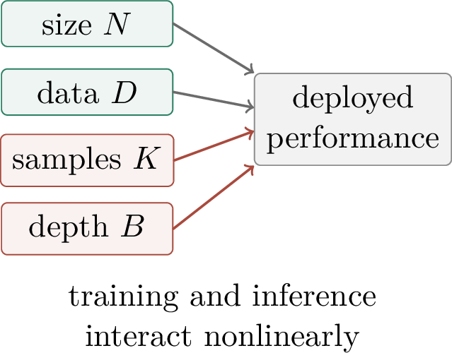
5.0.20.2 Thinking Versus Size
If extra inference compute raises solution probability more cheaply than increasing model size, a smaller model with more thinking can dominate. This is most plausible for hard problems with verifiable answers. Ambiguous or open-ended tasks may favor better base-model quality because there may be no cheap verifier or clear search objective.
This comparison is not simply small model versus large model. A larger base model may also make test-time compute more effective by producing more diverse high-quality candidates, better intermediate states, or more calibrated self-evaluations. Conversely, a smaller model may be easier to run many times under a latency or cost constraint. The frontier is a joint property of the base model and the inference policy.
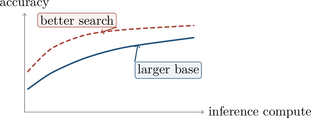
The policy must also know when to stop thinking. An adaptive test-time policy spends a low budget on easy queries and a high budget on hard ones. Calibration therefore becomes part of the scaling problem: the model must estimate whether extra computation is worth the latency and cost.
Adaptive inference can be formalized as a stopping problem. After each candidate, trace, or search expansion, the system observes some state information: confidence, verifier score, disagreement among samples, or remaining uncertainty. It should continue only if the expected improvement in deployment utility exceeds the marginal cost. Poor calibration wastes compute on easy queries and under-serves hard ones.
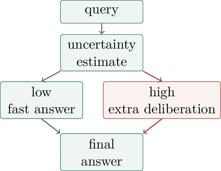
5.0.20.3 Qualitative Regimes
The return to test-time compute depends strongly on base skill. If the base model is too weak, sampling mostly repeats failures. At medium base skill, extra compute can have high leverage because some correct reasoning paths are within reach. At high base skill, returns saturate because many queries are already solved with little extra work.
This explains why inference scaling often looks task-dependent. A model may be in the high-leverage regime for competition math but already saturated on simple factual questions, or too weak for a long-horizon planning benchmark. Consequently, a single global “test-time scaling exponent” is less stable than a family of exponents indexed by task, verifier, and inference policy.
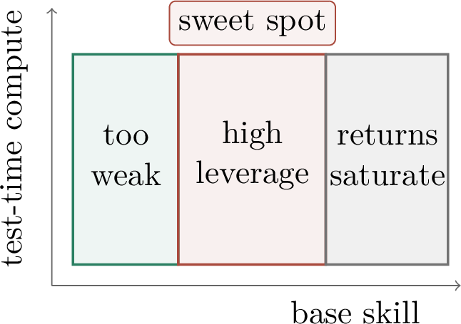
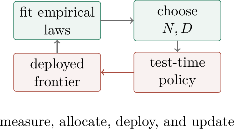
5.0.21 Limitations and Outlook↩︎
5.0.21.1 What Scaling Laws Miss
Scaling laws summarize average behavior in a controlled experimental family. They may miss rare failures, adversarial robustness, safety constraints, distribution shift, data contamination, latency, memory, serving constraints, and qualitative changes in reasoning strategy. A deployment decision should therefore combine scaling predictions with stress tests and task-specific evaluation.
Average loss can also hide tail risk. A model whose mean performance improves smoothly may still fail catastrophically on rare safety-critical cases. Similarly, a policy that improves benchmark accuracy by sampling many answers may increase latency, energy use, or exposure to problematic outputs. Scaling analysis is therefore a component of evaluation, not a substitute for it.
Test-time compute has its own limits. Samples may be correlated; verifiers may be unreliable; search may optimize spurious reasoning; and easy questions may be harmed by overthinking. We do not yet have a general theory predicting when extra inference compute produces genuinely new information rather than repeated noise.
When test-time compute helps, one should ask which ingredient improved: candidate diversity, reasoning depth, verifier accuracy, or adaptive routing. The same pass-rate gain can arise from very different mechanisms. Separating these mechanisms is essential if one wants to extrapolate beyond the measured budget.
5.0.21.2 Connections and Synthesis
| Earlier topic | Connection to scaling and test-time compute |
|---|---|
| Approximation | model size controls representable functions |
| Generalization | token count controls estimation error and data quality |
| Optimization | training recipe changes the reachable frontier |
| Double descent | interpolation can coexist with useful scaling |
| Transformers | architecture determines per-token compute and context use |
| Diffusion and flow | sampling quality depends on solver and inference budget |
Example 0.16 (Compute-optimal exponents). Assume \[L(N,D)-L_{\infty} = A N^{-1/2}+B D^{-1/4}, \qquad ND=C.\] Using the balanced-allocation proposition with \(\alpha=1/2\) and \(\beta=1/4\), \[N_\star\propto C^{1/3}, \qquad D_\star\propto C^{2/3}.\] The slower-decaying data term receives more of the compute growth.
Validation loss often follows power laws in parameters, data, and compute over controlled regimes. The optimal model is not always the largest model; it balances model size and data. Sampling, search, and verification can improve reasoning, but their returns depend on base skill, diversity, verifier quality, and latency.
Chapter Synthesis
Scaling laws are empirical resource-performance models; they are useful only within controlled experimental regimes.
Power-law loss curves turn multiplicative increases in compute into approximately linear trends on log-log axes.
Compute-optimal training balances marginal returns from model size and data, and the optimal split depends on fitted exponents.
Spectral tails and effective dimension give one mechanism by which power-law learning curves can arise.
Test-time compute improves performance through sampling, deliberation, search, and verification, but only when diversity and selection quality are adequate.
Deployment requires joint scaling of training and inference budgets, plus constraints such as latency, verifier reliability, and tail risk.
Foundational scaling references include Hestness et al., Deep Learning Scaling is Predictable, Empirically, Kaplan et al., Scaling Laws for Neural Language Models [21], Henighan et al., Scaling Laws for Autoregressive Generative Modeling, Bahri et al., Explaining Neural Scaling Laws, Hoffmann et al., Training Compute-Optimal Large Language Models [54], and Muennighoff et al., Scaling Data-Constrained Language Models. For test-time compute, see Cobbe et al., Training Verifiers to Solve Math Word Problems, Wang et al., Self-Consistency Improves Chain of Thought Reasoning, Yao et al., Tree of Thoughts, Lightman et al., Let’s Verify Step by Step, Sardana et al., Beyond Chinchilla-Optimal, Brown et al., Large Language Monkeys, Snell et al., Scaling LLM Test-Time Compute Optimally, and Muennighoff et al., s1: Simple Test-Time Scaling.
Scaling laws are not only curves; they are a language for making resource tradeoffs explicit. The next theoretical challenge is to connect these empirical frontiers with mechanisms: circuits, sparse features, superposition, phase transitions, verifier training, process supervision, search policies, and latency-aware deployment.
5.0.22 From Predictions to Mechanisms↩︎
Modern language models and vision models are useful precisely because they learn internal algorithms that were not written by a programmer. This is also why they are hard to understand. A trained transformer may copy names, recall facts, refuse requests, solve code-completion tasks, or perform in-context learning, but the learned implementation is distributed across residual streams, attention heads, MLPs, and high-dimensional activation vectors.
Mechanistic interpretability asks for reverse engineering. Instead of being satisfied with the statement that a model predicts a token, we would like to know which internal variables caused the prediction, which components computed those variables, and how the computation would change under targeted interventions. The guiding question for this chapter is:
Can we replace “the model predicts this” by a faithful explanation of which internal features caused the prediction?
This question has two important qualifications. First, a mechanistic explanation is always relative to a behavior and a distribution of examples. Explaining why a model copies a name in one family of prompts does not automatically explain why it answers factual questions, writes code, or refuses unsafe requests. Second, the target is the trained model itself, not the human concept that the model appears to use. A model may implement a task using shortcuts, redundant pathways, or internal variables whose meaning only partially matches the label that a human assigns to them. Mechanistic interpretability therefore treats the network as an object of empirical mathematics: propose internal variables, derive predictions from them, and then intervene on the model to test those predictions.
Definition 0.87 (Mechanistic explanation). A mechanistic explanation of a model behavior is a description of internal variables and causal pathways that is localized, compositional, predictive on new examples, and testable by interventions. Localization means that the explanation points to components or features; compositionality means that the pieces can be assembled into a circuit; causality means that editing the claimed variables changes the behavior in the predicted way.
This standard is stricter than many familiar interpretability artifacts. Saliency maps, attention visualizations, natural-language rationales, and linear probes can be useful clues, but by themselves they are not mechanistic explanations. A probe may correlate with a concept without being used by the model. A rationale may sound plausible without matching the internal computation. A saliency map may reveal sensitivity but not the algorithm. Mechanistic work therefore pairs observation with causal tests.
The distinction is analogous to the difference between fitting a black-box regression model and identifying a causal mechanism. A behavioral description summarizes the input-output relation; a mechanistic explanation tries to name the intermediate variables that make the relation happen. The circuits program initiated by Olah and collaborators emphasizes exactly this stronger standard: explanations should be local enough to inspect, compositional enough to combine, and causal enough to survive interventions [22]. In modern transformer language models, the same principle is harder to apply because the relevant variables may be distributed across many layers and positions.
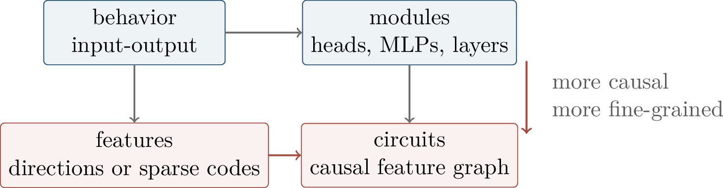
The chapter follows the route in 286. We first review circuits and interventions. We then study superposition, the hypothesis that models pack more features than available coordinates by representing features as non-orthogonal directions. Sparse autoencoders are introduced as a method for recovering candidate feature coordinates. The final sections explain how to build feature circuits and how to evaluate their limitations.
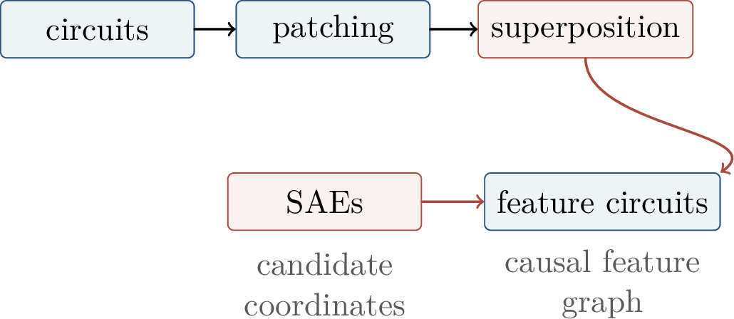
5.0.23 Circuits and Interventions↩︎
5.0.23.1 Residual Streams and Features
Let \(x_{1:T}\) be a token sequence and let \(r_\ell(t)\in\R^d\) denote the residual stream at layer \(\ell\) and position \(t\). In a simplified pre-normalization transformer block, the next residual stream is written as \[r_{\ell+1}(t) = r_\ell(t) + \operatorname{Attn}_\ell(r_\ell)_t + \operatorname{MLP}_\ell(r_\ell(t)). \label{eq:ch16-residual-stream}\tag{2}\] The residual stream is a shared communication channel. Attention heads read from positions, write vectors back into this channel, and MLPs perform token-wise nonlinear transformations. This additive form makes transformer circuits easier to discuss: components can be viewed as reading from and writing to a common vector space.
Equation 2 is intentionally schematic. Real transformer blocks include layer normalization, attention softmaxes, value and output projections, MLP nonlinearities, and sometimes architectural variants such as gated MLPs. The schematic form is still useful because it emphasizes one structural fact: many components contribute additively to a common residual stream. A component can therefore be studied by asking two questions. What information does it read from the current residual state? What direction, or collection of directions, does it write back for later components to use?
Definition 0.88 (Activation feature). An activation feature is a scalar coordinate or learned variable extracted from an activation. A linear feature at layer \(\ell\) and position \(t\) has the form \[z_f(x,t,\ell)=\left\langle v_f,r_\ell(t) \right\rangle,\] where \(v_f\in\R^d\) is a direction in the residual stream. More generally, the feature may be a learned sparse coordinate \(z_j=E_j(a)\) of an activation \(a\).
It is useful to separate components from features. A component is a place where computation happens, such as an attention head, an MLP neuron, or a residual-stream position. A feature is a computational variable represented in activations. A circuit connects features through components and residual paths.
This separation prevents a common confusion. Neurons and attention heads are architectural coordinates; features are hypotheses about variables used by the model. Sometimes a feature is close to a single neuron or a single direction, but often it is distributed over many coordinates. Conversely, a single coordinate may participate in several features. For this reason, the goal is not simply to give every neuron an English name. The goal is to find variables whose changes have predictable downstream effects.
Definition 0.89 (Circuit). A circuit is a small directed subgraph of internal variables whose values are sufficient, under specified interventions, to reproduce a target behavior. The target behavior may be a logit difference, a classification decision, a copied token, or another scalar metric of interest.
The phrase “under specified interventions” is part of the definition, not a technical afterthought. A circuit claim should say what happens if one removes a node, replaces it by a baseline value, or inserts the corresponding value from another run. In this sense, a circuit is closer to a causal model than to a visualization. It is allowed to be approximate and local, but it should support counterfactual predictions: if this internal variable is changed while the rest of the computation is held fixed as much as possible, the behavior should change in a predicted direction.
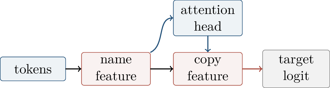
5.0.23.2 Activation Patching
Activation patching is the basic experimental tool for turning a circuit hypothesis into a causal test. Run the model on a clean input \(x\) where the behavior occurs and on a corrupted input \(\tilde{x}\) where the behavior is removed or changed. Then replace a chosen hidden state in the corrupted run by the corresponding hidden state from the clean run: \[r_\ell^{\mathrm{patch}}(t) = \begin{cases} r_\ell^{\mathrm{clean}}(t), & (\ell,t)\in S,\\ r_\ell^{\mathrm{corr}}(t), & (\ell,t)\notin S. \end{cases} \label{eq:ch16-activation-patching}\tag{3}\] The patch asks whether the clean hidden state carries the information that the corrupted run lost. If the behavior returns, then the patched state is causally relevant for that behavior on the tested distribution.
A practical patching experiment therefore has four ingredients. One chooses a clean input \(x\), a corrupted input \(\tilde{x}\), an internal site or set of sites \(S\), and a scalar metric \(m\). The metric should isolate the behavior of interest; for example, a logit difference between a correct token and a distractor is often more informative than the raw probability of one token. The corrupted input should remove the relevant information while leaving other aspects of the prompt as similar as possible. Otherwise a patch may recover the metric for an accidental reason rather than because it restores the intended variable.
Definition 0.90 (Patch score). Let \(F\) be the model and let \(m\) be a scalar behavior metric, such as a logit difference. The patch score of a set of internal states \(S\) is \[\Delta_S = m\big(F(\tilde{x}; r_S \leftarrow r_S(x))\big) -m(F(\tilde{x})).\] Large positive \(\Delta_S\) indicates that the patched states contain information that helps recover the clean behavior.
It is often useful to normalize the patch score by the clean-corrupted gap: \[\rho_S = \frac{ m\big(F(\tilde{x}; r_S\leftarrow r_S(x))\big)-m(F(\tilde{x})) }{ m(F(x))-m(F(\tilde{x})) }.\] When the denominator is positive and not too small, \(\rho_S\approx 1\) means that the patch recovers most of the clean behavior, whereas \(\rho_S\approx 0\) means that the patch has little effect. Values outside \([0,1]\) are possible: an intervention may overshoot the clean behavior or push the model in the opposite direction. Such cases are not mistakes in the definition; they are signals that the chosen site interacts nonlinearly with the rest of the computation.

Patching is most informative when the clean and corrupted inputs differ in a controlled way. For an induction-head experiment, a clean prompt may contain the pattern \(A\,B,\ldots,A\) so that the model should predict \(B\). A corrupted prompt changes the earlier occurrence and removes the relevant match. Patching then localizes where the model stores the match and where it copies the following token.
The result of a patch should be interpreted locally. A successful patch does not prove that the patched variable is the unique cause of the behavior, nor does a failed patch prove that the variable is irrelevant. The clean value may be incompatible with the corrupted context; several redundant circuits may exist; or the behavior may depend on a distributed subspace rather than on a single activation vector. For this reason, patching is strongest when it is combined with ablation, path patching, held-out prompt families, and control interventions that patch unrelated states.
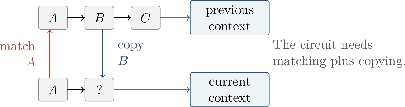
Strong evidence for a circuit comes from a pattern of interventions: patching restores the behavior, ablation destroys it, a simpler replacement circuit preserves it, and the effect transfers to held-out examples. The main risks are that correlated variables are patched together, the intervention creates off-distribution hidden states, multiple circuits implement the same behavior, or the proposed explanation covers only a narrow dataset.
Thus mechanistic claims should be falsifiable. A proposed circuit should make predictions about what will happen if a hidden state, feature, attention head, or MLP subspace is edited.
5.0.24 Superposition↩︎
5.0.24.1 Polysemanticity
A recurring obstacle is polysemanticity: individual neurons often fire for several unrelated concepts. One neuron may respond to city names, date formats, programming-language tokens, and proper names, depending on context. This is not necessarily a training failure. It may be an efficient coding strategy under dimension pressure.
The superposition viewpoint, developed in toy models by Elhage and collaborators, proposes that networks can represent many sparse features in a smaller number of activation dimensions by using non-orthogonal feature directions [55]. In this view, a neuron is polysemantic because the coordinate axes chosen by the architecture need not match the feature directions chosen by training. A single coordinate can cut across several meaningful directions, just as a two-dimensional projection of a high-dimensional sparse code can mix several variables.
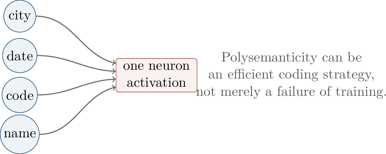
The central question is whether \(n>d\) useful features can be represented reliably in a \(d\)-dimensional hidden space. Superposition answers yes, under sparsity and tolerance for some interference.
The two qualifiers are essential. Sparsity means that only a small subset of features is active on any given input, so most potential collisions do not occur at the same time. Tolerance for interference means that exact recovery of every feature is not required; the model only needs errors small enough not to damage the downstream objective. These conditions explain why rare features are natural candidates for superposition, while frequent or safety-critical features may require cleaner directions.
5.0.24.2 A Toy Model
Let \(x\in\R^n\) be a vector of sparse nonnegative features, and suppose a model must represent these features in a lower-dimensional hidden space \(\R^d\), where \(d<n\). A simple autoencoding model is \[h = W x,\qquad \hat{x}=\sigma(W^\top h+b), \label{eq:ch16-superposition-toy}\tag{4}\] where \(W\in\R^{d\times n}\), the column \(w_i\) is the hidden-space direction for feature \(i\), and \(\sigma\) enforces nonnegativity. With feature importances \(s_i>0\), a typical objective is \[\min_{W,b}\; \E_x\sum_{i=1}^n s_i(\hat{x}_i-x_i)^2 \quad\text{subject to}\quad W\in\R^{d\times n}. \label{eq:ch16-toy-objective}\tag{5}\]
The columns of \(W\) are feature directions sharing a smaller hidden space. If \(n\le d\), the easiest solution is to place important features in nearly orthogonal directions. If \(n>d\), the model must choose which features get dedicated dimensions and which features are packed into superposition.
To see the interference explicitly, suppose for a moment that the nonlinearity and bias do not change the sign of the relevant decoded coordinate and that the feature directions are normalized. Projecting the hidden representation onto \(w_i\) gives \[\left\langle w_i,h \right\rangle = \left\langle w_i,Wx \right\rangle = x_i+\sum_{j\ne i}\left\langle w_i,w_j \right\rangle x_j .\] The first term is the desired feature value. The remaining terms are cross-talk from other active features. Orthogonal directions eliminate cross-talk, but exact orthogonality for all \(n\) features is impossible when \(n>d\). Superposition accepts small cross-talk in exchange for representing more features than the hidden dimension would otherwise permit.
Suppose at most \(k\) out of \(n\) features are active on a typical input, with \(k\ll n\). If the feature directions are nearly orthogonal on active sets, then decoding can tolerate \(n>d\) feature directions in \(d\) hidden dimensions.
Proof idea. When feature \(i\) is decoded by projecting onto \(w_i\), the signal term is approximately \(x_i\). The interference term has the form \[\sum_{j\ne i}\left\langle w_i,w_j \right\rangle x_j .\] Sparsity removes most terms because most \(x_j\)’s are zero. If the remaining active directions have small, balanced inner products with \(w_i\), then the total interference is small compared with the signal. Thus the model can store more feature directions than coordinate axes, provided that features are rare enough and interference is acceptable. ◻
This calculation reveals the tradeoff. Dense features, high-importance features, and features requiring low error tend to receive cleaner directions. Rare or low-importance features are cheaper to pack into superposition.
One can also phrase the tradeoff probabilistically. If feature \(j\) is active with probability \(p_j\), then the expected interference affecting coordinate \(i\) depends not only on the inner products \(\left\langle w_i,w_j \right\rangle\) but also on how often the interfering features are present. A rare feature can share a directional neighborhood with other rare features because their simultaneous activation is uncommon. A frequent feature collides with many examples and therefore pays a higher loss for the same geometric interference.
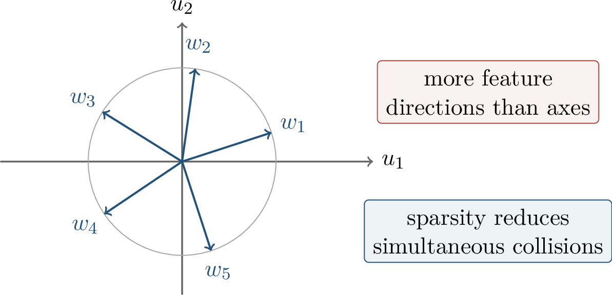
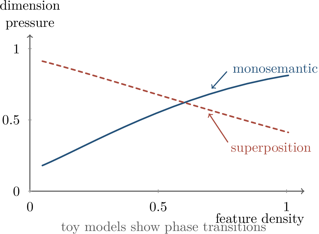
Superposition can be understood as compression. It lets a model store many rare features, use limited residual dimensions efficiently, and build distributed codes. Its cost is that neurons and directions become entangled: individual neurons may be polysemantic, causal edits may affect several features at once, and feature recovery requires additional assumptions. Sparse autoencoders are motivated by the hypothesis that dense activations are sparse combinations of many more meaningful feature directions.
The phase diagram in 292 should be read as a conceptual map rather than a theorem about every layer of every model. Real networks contain nonlinearities, normalization, attention routing, and task-dependent losses. The lesson is more modest but still important: monosemanticity is not guaranteed by architecture, and polysemanticity may be a rational consequence of optimization under finite-dimensional constraints.
5.0.25 Sparse Autoencoders↩︎
5.0.25.1 Dictionary Learning View
Collect activations \(a\in\R^d\) from a layer, residual stream, or MLP activation space. The dictionary-learning hypothesis says that these activations can be approximated as \[a \approx D z + b,\qquad D=[d_1,\ldots,d_m]\in\R^{d\times m},\qquad m\gg d, \label{eq:ch16-dictionary}\tag{6}\] where \(z\in\R^m\) is sparse. The columns \(d_j\) are candidate feature directions, and the coefficients \(z_j(a)\) are candidate feature activations. This is the same basic mathematical template that underlies classical sparse coding, but here the data points are internal neural-network activations rather than images, audio signals, or hand-designed features. The modern monosemantic-feature program uses this template to search for coordinates that are more semantically and causally coherent than raw neurons [56].
The overcomplete case \(m\gg d\) is essential. If superposition is real, then there may be many more features than dimensions in the original activation space. The hope is that only a few features are active on each token, so an overcomplete sparse code can represent the activation without forcing every coordinate to be active all the time.
There are unavoidable non-identifiabilities. The order of the dictionary columns is arbitrary. A decoder column can be rescaled if the corresponding code coordinate is inversely rescaled, unless a normalization convention or regularization fixes the scale. If two true features always co-occur in the activation dataset, no unsupervised reconstruction objective can reliably separate them without additional assumptions. Thus an SAE should not be understood as revealing “the” unique feature basis. It proposes a useful coordinate system whose scientific status must be tested.
Definition 0.91 (Sparse autoencoder). Given activations \(a\), a sparse autoencoder consists of an encoder \(E\) and a decoder \(D_{\mathrm{dec}}\). A common one-layer form is \[z = E(a)=\relu\big(W_e(a-b_e)+c_e\big), \qquad \hat{a}=D_{\mathrm{dec}}(z)=W_dz+b_d.\] It is trained by minimizing a reconstruction-sparsity objective such as \[\min_{E,D_{\mathrm{dec}}} \E_a\left[\left\lVert a-\hat{a} \right\rVert_2^2+\lambda\left\lVert z \right\rVert_1\right]. \label{eq:ch16-sae-objective}\qquad{(1)}\] The columns of \(W_d\) are candidate feature directions, while the coordinates \(z_j\) are candidate feature activations.
The reconstruction term and sparsity term play complementary roles. The reconstruction term prevents the encoder from inventing sparse labels that do not preserve the original activation. The \(\ell_1\) term prevents the model from using many small coordinates on every example. In practice, implementations often normalize decoder columns, monitor the fraction of active features, and check reconstruction on held-out activations. These details matter because a low training loss alone does not imply interpretability.
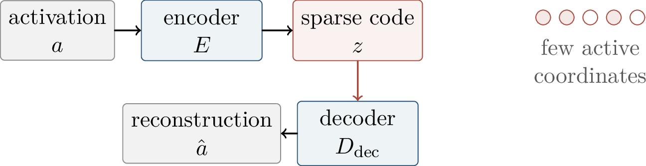
5.0.25.2 Why Sparsity Helps
Without sparsity, the decomposition \(a=\sum_{j=1}^m d_jz_j\) has many equivalent solutions. If a dense code reconstructs well, a rotated dense code may reconstruct equally well, so the coordinates need not correspond to stable concepts. Sparsity breaks much of this rotational symmetry. It prefers explanations that reuse a small number of directions across examples, which is exactly the behavior desired from interpretable features.
A simple example illustrates the problem. Suppose two coordinates are always used densely. Then replacing them by any orthogonal rotation of the same two-dimensional subspace may preserve reconstruction error, but the individual rotated coordinates need not have stable meanings. If, instead, examples tend to activate one coordinate at a time, most rotations destroy sparsity. The sparse coordinate system is then singled out by the data distribution. This is the intuitive reason that sparse penalties can turn an otherwise arbitrary basis into candidate features.
Lemma 0.27 (Sparse recovery intuition). Assume an activation has the ideal form \(a=Dz^\star\), where \(z^\star\) is \(k\)-sparse, the dictionary columns are normalized, and the dictionary coherence \[\mu=\max_{i\ne j}\left\lvert \left\langle d_i,d_j \right\rangle \right\rvert\] is small. If \(k\mu\) is sufficiently small, then an \(\ell_1\)-regularized reconstruction objective can identify the sparse support.
Proof sketch. Low coherence means that no small group of incorrect atoms can mimic a true active atom. The reconstruction term asks the code to explain \(a\), while the \(\ell_1\) penalty discourages dense alternatives. In the classical noiseless linear setting, coherence conditions imply uniqueness of the sparsest representation and recovery by convex relaxation. SAE training is more complicated because the encoder is learned, activations are noisy, and the true dictionary is not given; nevertheless the same geometry explains why sparsity is helpful. ◻
This lemma is deliberately stated as intuition rather than as a complete SAE recovery theorem. Classical sparse recovery assumes a fixed dictionary and a well-specified data model. In mechanistic interpretability, both the dictionary and the encoder are learned from activations produced by a nonlinear network. The useful takeaway is the geometric one: sparse, low-coherence decompositions are easier to interpret than dense, highly entangled decompositions.
The sparsity level is controlled by the penalty \(\lambda\), the dictionary size \(m\), the encoder architecture, activation normalization, and training heuristics. Too little sparsity mixes features. Too much sparsity discards information and produces poor reconstructions.
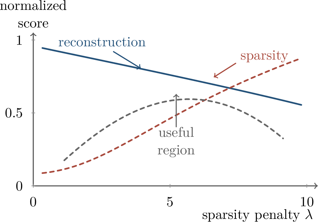
Several training choices matter in practice: which layer and token positions provide activations, whether the residual stream or an MLP activation is used, the expansion factor \(m/d\), whether encoder and decoder weights are tied, the sparse penalty schedule, activation normalization, dead-feature resampling, and held-out reconstruction tests. An SAE is best viewed as a feature proposal. Semantic and causal validation are still required.
A good workflow separates three questions. The representation question asks whether the SAE reconstructs activations with a sparse code. The semantic question asks whether individual coordinates have coherent top-activating examples and meaningful counterexamples. The causal question asks whether editing those coordinates changes model behavior in the predicted way. The last question is the hardest and is the one that turns a feature dictionary into mechanistic evidence.
5.0.26 Feature Circuits↩︎
5.0.26.1 From Neurons to Sparse Features
Once an SAE has proposed sparse coordinates, the interpretability target shifts from neurons to features. Instead of saying that a dense residual vector is important, we can ask which sparse coordinates were active, which downstream features they influenced, and which logits they affected.
This shift changes the unit of analysis. A neuron-level graph has nodes that are built into the architecture, but those nodes may be polysemantic. A feature-level graph has nodes learned by the interpreter, so the graph may be more meaningful but also more dependent on the dictionary-learning procedure. The correct attitude is therefore experimental: feature graphs are hypotheses about computation, not direct readouts of the model’s source code.
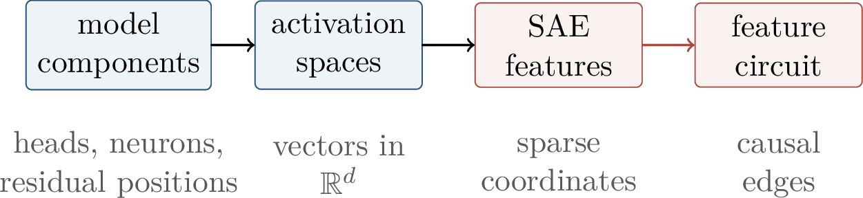
For a scalar logit or score \(y\), local linearization gives a first-order attribution formula: \[\Delta y \approx \sum_j \frac{\partial y}{\partial z_j}\Delta z_j . \label{eq:ch16-feature-attribution}\tag{7}\] A feature \(j\) is a positive contributor on an example if \(z_j\) is active and \(\partial y/\partial z_j\) is large and positive. It is inhibitory if the derivative is negative. Attribution is only local, so it should be used to generate hypotheses rather than to certify a circuit.
Formula 7 is the first-order Taylor expansion of \(y\) as a function of the sparse coordinates. It is reliable only when the perturbation \(\Delta z\) is small enough that higher-order terms are negligible and when changing \(z_j\) corresponds to a meaningful change in the original activation space. These conditions can fail in transformers because attention patterns, nonlinear gates, and normalization statistics may change after an intervention. Thus large attribution scores are best treated as a shortlist of candidate edges that should be checked by patching or ablation.
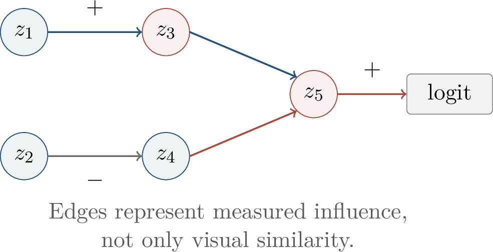
5.0.26.2 Steering, Ablation, and Iteration
Feature interventions make the causal test explicit. In an ablation, one sets a feature activation to zero, \[z_j \leftarrow 0,\] and measures whether the behavior disappears. In steering, one adds a decoder direction to an activation, \[a \leftarrow a+\alpha d_j,\] and measures whether the behavior appears or changes predictably. Ablation suggests necessity on a distribution; steering suggests sufficiency in a context. Both can create off-distribution activations, so their effects should be tested across many prompts and compared with controls.
The distinction between necessity and sufficiency is useful. If ablating feature \(j\) destroys a behavior, then \(j\) was necessary for that behavior under the tested conditions, but another feature might compensate on a different distribution. If adding \(\alpha d_j\) induces the behavior, then the feature direction can be sufficient in that context, but the intervention may have bypassed the normal upstream computation that would have created the feature. A robust explanation tries to connect both sides: upstream features produce \(z_j\), \(z_j\) contributes to downstream features, and the whole path generalizes across examples.
Example 0.17 (A monosemantic feature claim). A feature is plausibly monosemantic when its top activating examples share a coherent concept, it is sparse across unrelated contexts, its activation predicts downstream behavior, and ablation or steering changes that behavior as expected. A typical claim might be: a feature activates for references to a programming language, contributes to code-completion logits, and steering it increases code-like continuations. The semantic label is not the evidence by itself; the evidence is the combination of activation statistics, transfer, and causal effects.
This view connects directly to earlier chapters. Local feature attribution is a first-order linearization, echoing the NTK perspective. Sparsity and dictionary geometry are implicit biases in the explanation method. A useful explanation must generalize beyond the examples that revealed it. Robustness questions reappear because causal features can expose brittle shortcuts or adversarial directions. Scaling questions reappear because larger models may have both more specialized features and more distributed circuits.
There is also a design lesson. If a feature circuit reveals that a model uses a brittle shortcut, then the explanation can suggest new data, new evaluations, or new regularizers. If a feature circuit reveals a robust internal algorithm, then it can support more targeted monitoring and debugging. Interpretability is therefore not only a post-hoc descriptive activity; in favorable cases it feeds back into model evaluation and training.
5.0.27 Evaluation and Limits↩︎
5.0.27.1 Criteria for Explanations
A useful explanation must balance three requirements. It should be faithful to the model computation, legible enough for humans to inspect, and broad enough to transfer across examples. Any two requirements are insufficient. A dictionary can be sparse and semantically attractive while failing to mediate the behavior. A faithful circuit can be too large to understand. A circuit can work on a benchmark slice but fail elsewhere.
Faithfulness is the non-negotiable scientific requirement: the explanation must track the computation actually used by the model. Legibility is the human-facing requirement: the explanation should be simple enough that a researcher can inspect it, name it, and notice when it behaves unexpectedly. Coverage is the statistical requirement: the explanation should remain useful outside the few examples on which it was discovered. The tension among these requirements explains why mechanistic interpretability is difficult. A tiny hand-labeled circuit may be legible but incomplete; a massive automatically extracted graph may be faithful but unreadable; a feature label may transfer well semantically while failing a causal test.
Representation metrics include reconstruction error, fraction of variance explained, average active features, feature activation frequency, and the dead-feature rate. Mechanistic metrics include causal ablation effects, steering consistency, transfer across prompts, circuit completeness, and sensitivity to dictionary size. Good representation metrics are necessary for an SAE to be useful, but they do not imply that the discovered features explain a particular behavior.
This distinction is especially important when comparing SAE runs. A larger dictionary may improve reconstruction while splitting one human concept across several features. A stronger sparsity penalty may make features look cleaner while losing information needed for causal faithfulness. A feature with a beautiful top-activation dashboard may still be irrelevant to the behavior under study. Evaluation must therefore include both representation-level and behavior-level tests.
Definition 0.92 (Completeness test). Given an explanation \(E\) for a behavior metric \(m\), a completeness test replaces internal variables outside \(E\) by values sampled from a baseline distribution. If \(m\) is preserved, then \(E\) is approximately complete for that behavior under the tested intervention distribution.
Completeness tests whether the proposed variables carry enough information to compute the behavior after nuisance variation is removed. They do not prove uniqueness. Multiple circuits may implement the same input-output behavior, and preserving one metric may hide changes in other behaviors.
One should also distinguish completeness from minimality. A complete explanation may contain redundant variables, while a minimal explanation may omit variables that matter on rare inputs. In safety applications the second failure can be more serious: a circuit that explains average behavior may miss an internal pathway that activates only under adversarial or unusual prompts. For this reason, completeness tests should be paired with stress tests on prompt families designed to expose alternative mechanisms.
5.0.27.2 Failure Modes
Sparse autoencoders can produce convincing-looking features. The scientific burden is to show that these features faithfully mediate behavior rather than merely offering a pleasing decomposition of activation space.
The main theoretical questions are still open. First, under what distributional and architectural assumptions is an SAE dictionary identifiable up to permutation and scaling? Second, when does a feature-level causal graph approximate the true nonlinear computation of a transformer? Third, do larger models become more interpretable because features specialize, or less interpretable because circuits become more distributed?
These questions mark the boundary between current empirical practice and a future theory of interpretability. The existence of useful sparse features in some models does not imply that every behavior admits a compact feature circuit. Conversely, failure to find a clean SAE feature does not prove that the model lacks a meaningful internal variable; the chosen layer, dictionary size, sparsity penalty, or dataset may be wrong. Negative results are most informative when the search procedure and evaluation metrics are stated precisely.
The current research frontier includes automated interpretability, cross-layer dictionaries, sparse feature circuits, circuit tracing, and safety applications such as detecting hidden objectives, jailbreak mechanisms, or deceptive features. The field has promising tools, but no general theorem yet says that recovered features are the unique and complete internal ontology of a model.
5.0.28 Summary↩︎
Mechanistic interpretability seeks causal explanations of internal computation. Activation patching and ablation turn interpretability hypotheses into interventions. Superposition explains why neurons can be polysemantic under dimension pressure. Sparse autoencoders try to recover a sparse feature basis from dense activations. A feature is scientifically useful only when semantic interpretation is paired with causal validation.
Chapter Synthesis
Mechanistic interpretability aims to explain a trained model’s behavior in terms of internal variables and causal pathways, not merely correlations or plausible verbal rationales.
Transformer residual streams provide a shared communication channel in which attention heads, MLPs, and sparse features can be studied as readers and writers of information.
Activation patching, ablation, and steering are intervention tools: they test whether proposed internal variables are necessary, sufficient, or causally relevant for a behavior on a specified distribution.
Superposition explains how many sparse features can share fewer activation dimensions, at the cost of interference and polysemantic neurons.
Sparse autoencoders turn dense activations into overcomplete sparse codes, producing candidate features that require semantic and causal validation.
Evaluation must balance faithfulness, human legibility, and coverage; good reconstruction metrics alone do not establish a complete mechanistic explanation.
For general neural-network and sparse-coding background, see Goodfellow, Bengio, and Courville [29] and Bishop [57]. Core mechanistic-interpretability sources include Olah et al., Zoom In: An Introduction to Circuits [22]; Elhage et al., A Mathematical Framework for Transformer Circuits; Elhage et al., In-Context Learning and Induction Heads; Meng et al., Locating and Editing Factual Associations in GPT; Elhage et al., Toy Models of Superposition [55]; Bricken et al., Towards Monosemanticity [56]; Cunningham et al., Sparse Autoencoders Find Highly Interpretable Features in Language Models; Templeton et al., Scaling Monosemanticity; and Anthropic, Circuit Tracing.
The next step is to connect interpretability with design and evaluation. If we can identify reliable features and circuits, then we can audit model behavior, understand failure modes, and eventually ask whether training itself can encourage internal representations that are easier to inspect.
5.0.29 The Grokking Puzzle↩︎
In ordinary overfitting, training accuracy improves while test accuracy worsens. Grokking is stranger. A model first memorizes the training set, sits for a long time on a plateau where test accuracy is poor, and only much later discovers a rule that generalizes. The phenomenon is important because it links optimization, implicit regularization, representation learning, and phase-transition-like behavior in a setting where the correct rule can often be understood mechanistically. The original demonstrations of grokking used small algorithmic datasets and overparameterized networks, where the model can fit a finite table long before it learns the compact rule behind the table [23].
This makes grokking a useful microscope for generalization theory. In many large-scale tasks we do not know the exact rule, so it is hard to say whether a model has truly learned a reusable mechanism or merely exploited correlations in the dataset. In modular arithmetic, parity-like tasks, and other finite algorithmic worlds, the target rule is known. We can therefore compare three objects directly: the training loss, the test behavior on unseen inputs, and internal representations that should appear if the model has found the rule.
The guiding question is:
What changes during the long plateau before test accuracy rises?
The answer cannot be obtained from training accuracy alone. Once the model interpolates the training set, the external loss may look nearly solved, while hidden representation statistics continue to move.
The word “grokking” should not be used for every late improvement in a validation curve. The characteristic signature is a separation of time scales: interpolation happens first, then there is a long period in which visible test accuracy remains poor, and finally a generalizing solution appears. If test performance improves gradually together with training performance, the run may still be interesting, but it is not the same phenomenon. Conversely, if test accuracy jumps because a noisy or thresholded metric has crossed a reporting boundary, one must check whether the internal mechanism actually changed.
Definition 0.93 (Grokking phenomenology). A training run exhibits grokking when it reaches near-perfect training accuracy at time \(t_{\mathrm{train}}\), while near-perfect test accuracy appears only after a much larger time \(t_{\mathrm{test}}\): \[1\ll t_{\mathrm{train}}\ll t_{\mathrm{test}},\qquad \mathrm{acc}_{\mathrm{train}}(t_{\mathrm{train}})\approx 1,\quad \mathrm{acc}_{\mathrm{test}}(t_{\mathrm{test}})\approx 1.\] The phenomenon is not just a high final test accuracy; it is the large delay between interpolation and generalization.
The threshold used to define \(t_{\mathrm{train}}\) and \(t_{\mathrm{test}}\) is a measurement choice. For classification accuracy, changing the threshold from \(0.95\) to \(0.99\) can change the reported delay. For this reason, grokking experiments should also report continuous quantities such as cross-entropy, margins, weight norms, representation alignment, and circuit scores. These quantities often reveal whether the model is truly stalled or whether it is making slow hidden progress.
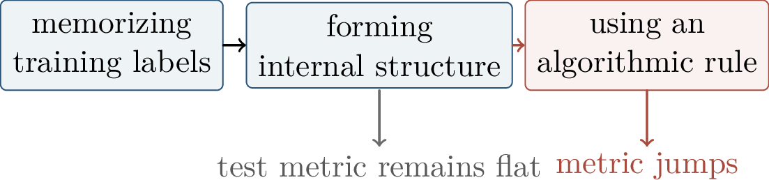
Grokking is a meeting point of themes from earlier chapters. Optimization dynamics determine whether the model keeps moving after interpolation. Implicit regularization selects among many interpolating solutions. Fourier structure explains compact algorithms for cyclic tasks. Double descent reminds us that interpolation is not the end of generalization. Mechanistic interpretability supplies internal progress measures.
This chapter will use “phase transition” language carefully. A sharp change in a plotted metric is evidence of a regime change only after one rules out measurement artifacts and finite-size effects. In a finite training run, all observed curves are finite-sample curves. The scientific content comes from identifying an order parameter, showing that it tracks an interpretable mechanism, and testing whether its transition becomes sharper or more stable under controlled changes of data, width, regularization, or compute.
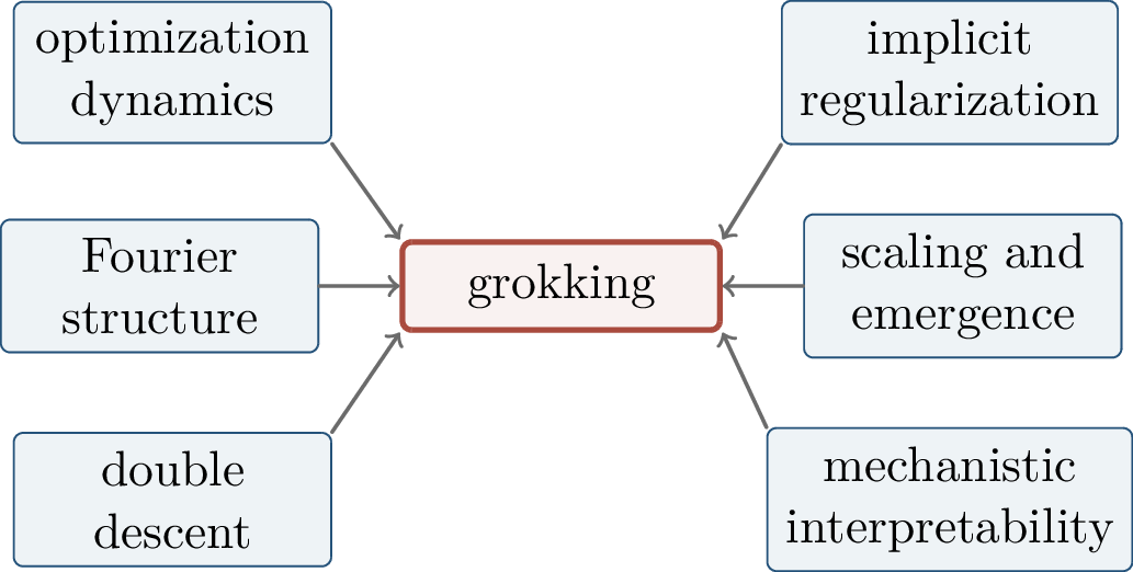
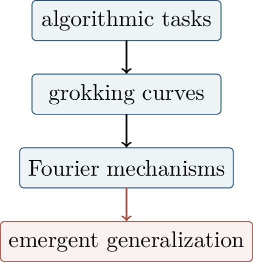
5.0.30 Setup and Algorithmic Tasks↩︎
5.0.30.1 Supervised Learning View
Let \((x,y)\sim\mathcal{D}\) and train a model \(f_\theta:\mathcal{X}\to\mathcal{Y}\) on \[S=\{(x_i,y_i)\}_{i=1}^n,\qquad \widehat{\mathcal{R}}_S(\theta) = \frac{1}{n}\sum_{i=1}^n \ell(f_\theta(x_i),y_i).\] The population risk is \[\mathcal{R}(\theta)=\E_{(x,y)\sim\mathcal{D}}\ell(f_\theta(x),y).\] Interpolation means \(\widehat{\mathcal{R}}_S(\theta)\approx0\). The grokking puzzle is that interpolation can happen early, while population performance waits for many more gradient steps.
For finite algorithmic tasks, \(\mathcal{D}\) is often the uniform distribution on all valid input-output pairs. The train set \(S\) is a random subset, and the test set is the complement. This removes one source of ambiguity: there is no distribution shift between train and test, only missing entries of a finite table. If a model fails on the complement after interpolating \(S\), it is not because the test inputs came from a different distribution. It is because the interpolating solution did not yet capture the rule that generated the table.
The same training loss can therefore correspond to qualitatively different predictors. A lookup-table solution stores the labels of the sampled pairs. A rule-based solution computes a function that is valid on every pair. Grokking asks why gradient-based training may first find the lookup-like solution and only much later move toward the rule-like solution.
5.0.30.2 Modular Addition
The canonical toy world is modular addition. For a prime \(p\), the task is \[(a,b)\longmapsto y=a+b \pmod p, \qquad a,b,y\in\mathbb{Z}_p .\] The domain is finite, so a sufficiently flexible network can memorize a random training split. Yet the true rule is compact and perfectly generalizing: addition is translation on a cyclic group.
The size contrast is useful. The full table has \(p^2\) input pairs, while the rule \(a+b \pmod p\) is described by one shared operation. A memorizing model can assign unrelated parameters or features to many observed pairs. A rule-learning model must represent the cyclic structure of \(\mathbb{Z}_p\), reuse it across all inputs, and produce the same output on examples that were never shown during training.
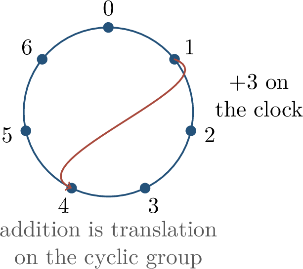
Two predictors can have the same training loss but very different test behavior. A memorizing solution stores observed labels with little reusable structure. An algorithmic solution represents the periodic rule and applies one computation to unseen pairs.
Example 0.18 (Lookup versus rule on \(\mathbb{Z}_5\)). Suppose the training set contains \((1,2)\mapsto3\), \((1,4)\mapsto0\), and \((3,4)\mapsto2\), all modulo \(5\). A lookup table can store these three labels and say nothing coherent about the unseen pair \((2,4)\). The rule solution, however, represents the operation \(a+b\pmod5\), so it immediately predicts \((2,4)\mapsto1\). Both predictors may have zero loss on the three training examples. Only the second predictor has learned a computation that extends across the group.
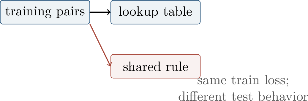
Definition 0.94 (Grokking delay). For a threshold \(0<\alpha<1\), define \[t_{\mathrm{train}}=\inf\{t:\mathrm{acc}_{\mathrm{train}}(t)\ge\alpha\},\qquad t_{\mathrm{test}}=\inf\{t:\mathrm{acc}_{\mathrm{test}}(t)\ge\alpha\}.\] The grokking delay is the ratio \(t_{\mathrm{test}}/t_{\mathrm{train}}\). A large delay means that hidden learning lasts long after the model fits the training set.
The ratio is crude but useful. It ignores the detailed shape of the loss curve, and it depends on the threshold \(\alpha\). Nevertheless, it captures the qualitative separation that makes grokking surprising. In ordinary generalization, one expects the same features that fit training examples to also help on similar test examples. In grokking, the training fit can be achieved by a mechanism that does not generalize, while the generalizing mechanism requires additional representation learning after the training metric is already saturated.
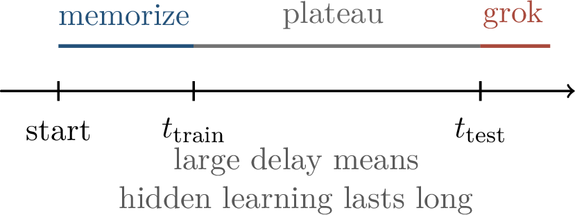
5.0.31 Curves and Phase Transitions↩︎
5.0.31.1 Canonical Curves
The canonical grokking curve has a rapid training-accuracy rise, a long plateau, and a late test-accuracy jump. Time is often plotted on a logarithmic scale because the delay can span orders of magnitude.
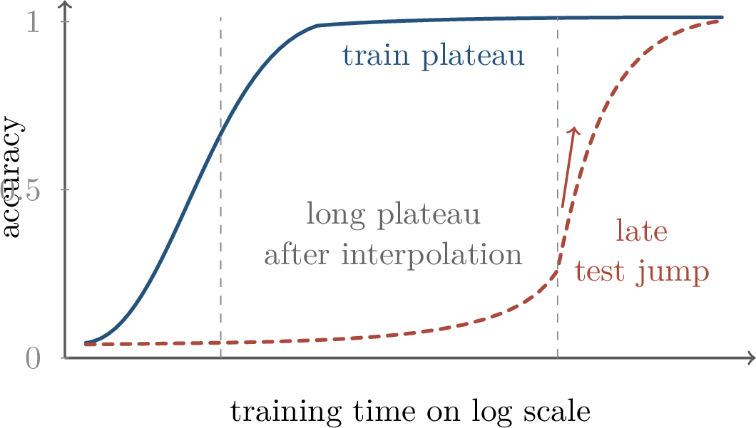
It is tempting to call this a phase transition. That language is useful only when one specifies a measurable statistic that behaves like an order parameter and shows sharper change as width, data, or compute grows.
In statistical physics, a phase transition is not merely a steep curve; it is a change in macroscopic behavior that becomes sharp in an appropriate limit. For grokking, there is usually no thermodynamic limit already built into the experiment. We therefore use the term operationally. A proposed phase transition should come with a statistic that distinguishes the memorizing regime from the rule-learning regime, and that statistic should be connected to the mechanism rather than only to final accuracy.
Definition 0.95 (Order parameter). An order parameter is a scalar statistic \(m(\theta)\) that is small in one regime and large in another: \[m(\theta)\approx0 \Rightarrow \text{memorizing},\qquad m(\theta)\approx1 \Rightarrow \text{structured rule}.\] Examples include alignment with known Fourier modes, strength of algorithmic features, effective rank, or a causal circuit score.
An order parameter is most convincing when it is not the metric being explained. If test accuracy is the only statistic that changes, then the transition may be a property of the benchmark. If a Fourier-alignment score, a representation rank, or a causal circuit score changes before the test metric jumps, then the transition has a more mechanistic interpretation. In modular addition this is possible because the correct harmonic structure is known in advance.
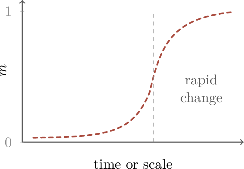
5.0.31.2 Hidden Progress
A central lesson from mechanistic analyses of grokking is that visible accuracy can be almost binary while internal statistics change smoothly. The model may slowly build sinusoidal embeddings, align logits with a Fourier circuit, or increase margins before the thresholded test metric records success. Nanda et al. use such progress measures to track the emergence of interpretable structure in modular addition models [58].
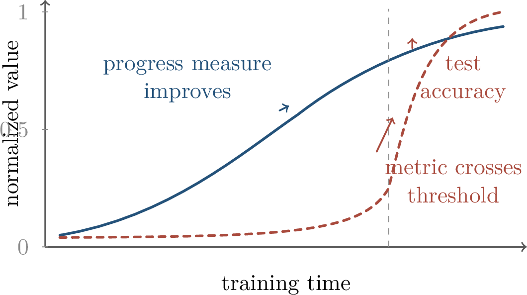
Suppose a latent score \(s(C)\) improves smoothly with compute or scale \(C\), but a benchmark reports \[A(C)=\mathbf{1}\{s(C)\ge \tau\}.\] Then \(A(C)\) can look discontinuous even when \(s(C)\) is smooth.
Proof. If \(s\) is continuous and crosses \(\tau\) at \(C_0\), then the indicator is zero for \(s(C)<\tau\) and one for \(s(C)\ge\tau\). Thus the reported metric jumps at \(C_0\) even though the underlying score may have changed gradually. The discontinuity is a property of the measurement map, not necessarily of the mechanism. ◻
This proposition is mathematically simple but conceptually important. Many reported abilities are thresholded: an answer is counted correct or incorrect, a proof either passes a checker or fails, a program either compiles or does not, and a multiple-choice answer is either the top logit or not. The latent quantity that improves during training may be a margin or probability assigned to the correct answer. Accuracy sees only the moment when that latent quantity crosses the decision boundary.
Accuracy is often the right final metric, but it is a poor diagnostic of hidden progress. A model whose correct-class probability rises from \(0.01\) to \(0.45\) on every test example may still have zero accuracy if the wrong class remains slightly larger. Cross-entropy, margin, calibration, and mechanistic alignment scores would reveal that the model has learned something substantial.
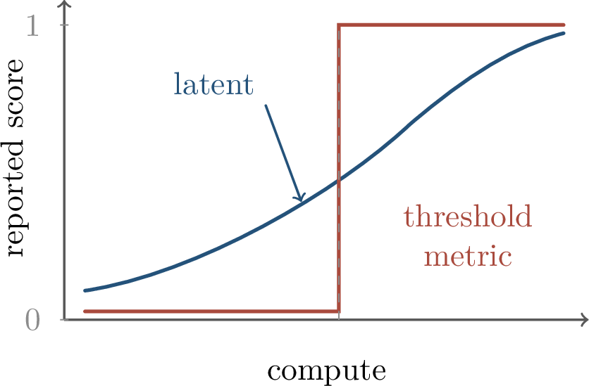
5.0.32 Mechanisms in Modular Arithmetic↩︎
5.0.32.1 Fourier Coordinates on \(\mathbb{Z}_p\)
The reason modular addition is analytically attractive is that the cyclic group has a simple Fourier basis. Let \[\omega=\exp(2\pi i/p).\] The Fourier characters on \(\mathbb{Z}_p\) are \[\chi_k(x)=\omega^{kx},\qquad k,x\in\mathbb{Z}_p.\] Every function \(g:\mathbb{Z}_p\to\mathbb{C}\) can be written as \[g(x)=\sum_{k\in\mathbb{Z}_p}\widehat g(k)\chi_k(x).\]
Lemma 0.28 (Translations are diagonal). Under the uniform measure on \(\mathbb{Z}_p\), the characters are orthonormal and diagonalize translation: \[\chi_k(x+c)=\chi_k(c)\chi_k(x).\]
Proof. The identity follows directly from the definition: \[\chi_k(x+c)=\omega^{k(x+c)}=\omega^{kc}\omega^{kx} =\chi_k(c)\chi_k(x).\] Orthonormality is the finite geometric-sum identity \[\frac{1}{p}\sum_{x\in\mathbb{Z}_p}\chi_k(x)\overline{\chi_{k'}(x)} = \frac{1}{p}\sum_{x\in\mathbb{Z}_p}\omega^{(k-k')x} = \mathbf{1}\{k=k'\}.\] ◻
For \(a,b\in\mathbb{Z}_p\), the key identity is \[\chi_k(a+b)=\chi_k(a)\chi_k(b).\] In real coordinates this becomes ordinary trigonometric addition, for example \[\cos(\alpha+\beta) = \cos\alpha\cos\beta-\sin\alpha\sin\beta.\] Thus the task looks like a table in input space but has low-dimensional harmonic structure in Fourier space.
The class indicator also has a compact Fourier expression. For a proposed answer \(y\in\mathbb{Z}_p\), \[\mathbf{1}\{a+b=y\} = \frac{1}{p}\sum_{k\in\mathbb{Z}_p} \chi_k(a+b-y) = \frac{1}{p}\sum_{k\in\mathbb{Z}_p} \chi_k(a)\chi_k(b)\overline{\chi_k(y)}.\] This identity follows from orthonormality: the average over all characters is one when \(a+b-y=0\) and zero otherwise. It shows that the whole \(p\times p\) addition table can be represented by shared harmonic features rather than by independent table entries. A neural network need not implement this formula literally, but mechanistic analyses look for internal variables that behave like its ingredients.
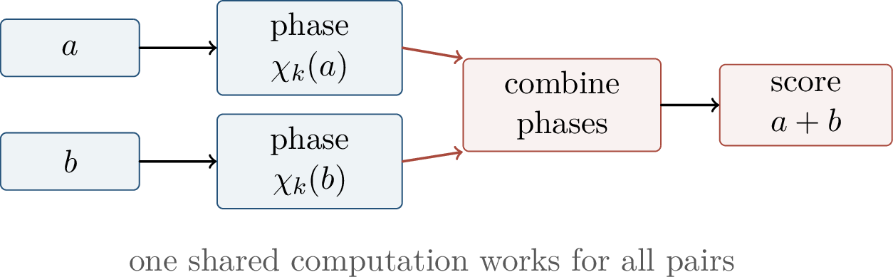
5.0.32.2 A Mechanistic Story
Mechanistic analyses of modular addition find internal variables that become more sinusoidal and more aligned with the correct Fourier modes before test accuracy jumps. The story is not that the network stores every pair \((a,b)\). Instead, embeddings gradually organize around circular features, the model combines these features trigonometrically, and the answer logits become aligned with the correct output.
This story gives content to the phrase “hidden progress.” Early in training, the model may fit observed pairs by using irregular features that do not respect the cyclic symmetry. During the plateau, these irregular features can weaken while harmonic features become stronger. The test accuracy remains low until the harmonic features are both present and connected to the output readout with sufficient margin. The late jump is then not the beginning of learning; it is the moment when a slowly forming mechanism becomes visible to the metric.
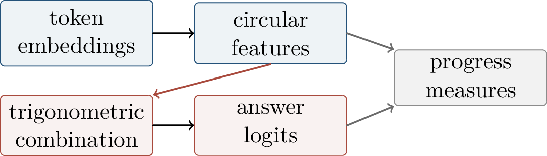
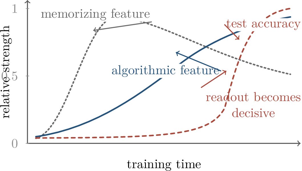
If a model constructs features approximating \(\chi_k(a)\) and \(\chi_k(b)\) for several \(k\), then a shallow readout can represent modular addition on all pairs using \[\chi_k(a+b)=\chi_k(a)\chi_k(b).\]
Proof sketch. Characters form a complete basis for functions on \(\mathbb{Z}_p\). Addition becomes multiplication of phases rather than storage of all \(p^2\) input pairs. A readout over the resulting phase features can concentrate score on the class \(y=a+b\pmod p\). This explains a compact solution class; it does not by itself prove that gradient descent must find it quickly. ◻
The last sentence is essential. Fourier analysis describes an efficient solution that exists in function space. Grokking concerns the path by which a specific architecture and optimizer find, delay, or fail to find that solution. Architecture matters because some parameterizations make harmonic features easy to represent; initialization matters because the right directions may start with tiny signal; regularization matters because it can favor shared features over memorized entries; and data fraction matters because the training split must contain enough evidence of the rule.
5.0.33 Regularization and Optimization↩︎
Many grokking experiments optimize a regularized objective \[\min_\theta\; \widehat{\mathcal{R}}_S(\theta)+\frac{\lambda}{2}\left\lVert \theta \right\rVert_2^2.\] After interpolation, the empirical loss is already small, but the regularizer can still reshape the solution. A memorizing solution fits \(S\) with many local degrees of freedom. An algorithmic solution reuses features. Late training can move along a low-loss manifold from the former toward the latter.
This description should be understood geometrically. The set of parameters with very small training loss is typically high-dimensional. Some directions inside this set preserve the labels of the training examples while changing norms, margins, and representations. If the empirical loss gradient becomes small but not exactly zero, and the weight-decay gradient remains present, optimization can continue to drift through this low-loss region. The drift is slow because it must avoid destroying interpolation, but it can be decisive for which predictor is selected.
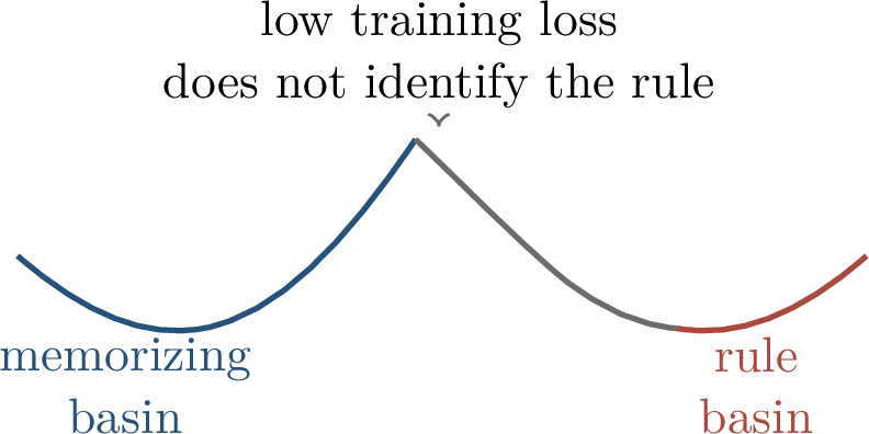
Suppose two interpolating predictors \(f_{\mathrm{mem}}\) and \(f_{\mathrm{rule}}\) satisfy \[\widehat{\mathcal{R}}_S(f_{\mathrm{mem}}) = \widehat{\mathcal{R}}_S(f_{\mathrm{rule}})=0,\qquad \Omega(f_{\mathrm{rule}})<\Omega(f_{\mathrm{mem}}).\] If training continues to decrease \(\Omega\) on the interpolation manifold, then the selected predictor can move from memorization toward the rule.
Proof sketch. Once empirical-loss gradients are small on \(S\), the regularizer can dominate the tangent dynamics along directions that preserve fit. The update direction then reduces complexity while keeping the training examples classified correctly. Shared representations are favored because they explain many examples with fewer effective degrees of freedom. ◻
This proposition is a schematic statement of an implicit-bias mechanism, not a complete theorem for deep networks. The complexity \(\Omega\) may be an explicit norm penalty, an implicit preference induced by the optimizer, or a combination of both. The claim is that among interpolating predictors, the rule can be simpler than memorization in the relevant geometry. Weight decay then helps only when the simpler predictor is reachable without losing the training fit.
This perspective is consistent with the distinction between lazy and rich training. In a lazy or kernel-like regime, features move little and the model fits examples with near-initial representations. In a rich regime, features reorganize, and the model can discover a more compact algorithm.
The lazy-to-rich distinction also clarifies why grokking can be delayed. A near-kernel solution may interpolate quickly because the network has enough random features to separate the training examples. However, those features are not arranged around the modular rule. Rich feature learning is slower because it requires coordinated movement of embeddings, hidden units, and readout weights. When the rich solution eventually has lower complexity or larger margin, the model can transition from the initial interpolating solution to a more structured one.
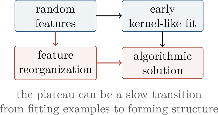
Several factors often shorten the grokking delay: stronger weight decay, more informative initialization, more data from the task distribution, architectures aligned with the algorithm, and optimization settings that preserve slow gradient signals. Conversely, weak regularization, excessive label noise, coarse metric thresholds, tasks with no compact rule, or stopping immediately after interpolation can hide grokking. The experimental lesson is simple: record train loss, test loss, norms, margins, and representation statistics, not only accuracy.
There is no single universal cause of grokking. In one experiment the delay may be controlled mostly by weight decay; in another, by data fraction or by the time needed for embeddings to become structured. This is why ablations are central. If increasing the train fraction removes the delay, then the rule may have been statistically underdetermined early on. If changing weight decay moves the transition time while preserving final accuracy, then late implicit regularization is likely important. If a structure-aware architecture groks quickly, then the original delay may have been representational rather than purely optimization-theoretic.
5.0.34 Emergent Generalization↩︎
5.0.34.1 Hidden Progress Beyond Modular Arithmetic
Delayed generalization is not limited to modular addition. For parity-like tasks, there are settings in which SGD can build weak target correlations before standard accuracy visibly improves.
The common pattern is a separation between information, representation, and readout. The data may contain weak statistical evidence of the target rule; the network may gradually organize that evidence into internal variables; and the output layer may only later convert those variables into correct predictions. A flat accuracy curve collapses these stages into one number. Grokking encourages us to instrument the intermediate stages.
Theorem 0.59 (Hidden progress, informal). For certain parity-like tasks, SGD can accumulate weak correlations with the target near the computational limit before a standard accuracy metric visibly improves.
Proof idea. Individual coordinates carry tiny signal, so a classifier built from any one coordinate is weak. SGD aggregates many weak correlations over time. A later readout step converts the accumulated signal into visible accuracy. Thus the absence of visible test improvement need not mean the absence of learning. ◻
This separates statistical availability from computational extraction. The data may contain enough information for the rule, but the optimization process must still discover a representation and readout that make the rule usable.
One should be cautious about the word “computational limit” in the informal theorem. The precise limit depends on the task distribution, architecture, optimizer, and amount of compute. The point is not that SGD always reaches the best possible algorithm. The point is that learning can proceed through weak signals that are invisible to coarse test metrics until the accumulated signal becomes usable by the final classifier.
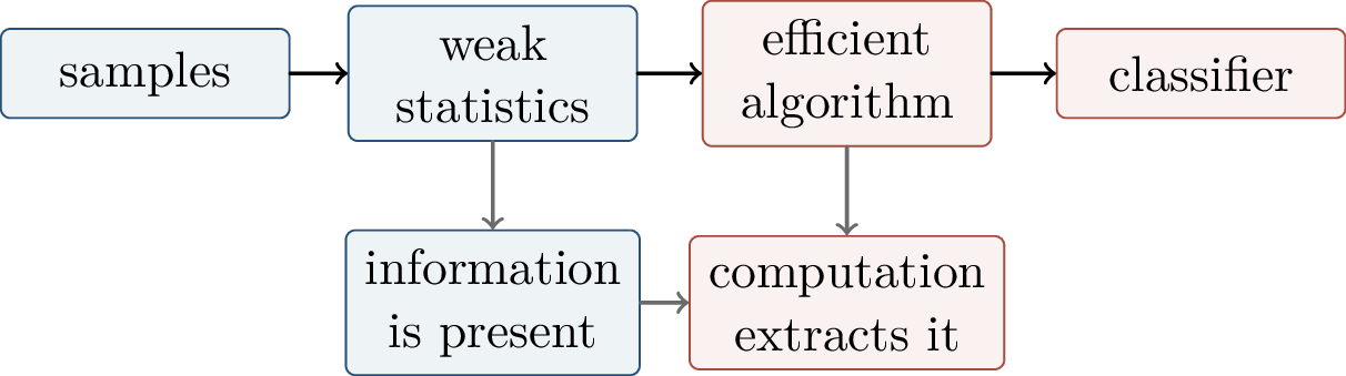
5.0.34.2 Emergence and Measurement
Large-model benchmarks often report emergent abilities: performance appears near chance for small scales and then jumps at a threshold. Grokking suggests two explanations. The first is a genuine mechanistic transition: a new internal algorithm becomes available. The second is a measurement transition: a smooth latent skill crosses a benchmark threshold. Both possibilities are discussed in the literature on emergent abilities and their measurement [59], [60].
The two explanations are not mutually exclusive. A model may gradually learn several prerequisite features, then combine them into a new circuit, and the benchmark may still report only a final pass/fail jump. Conversely, a model may improve smoothly at the level of log probability or margin, while exact match accuracy makes the curve look discontinuous. Distinguishing these cases requires more than plotting accuracy against scale.
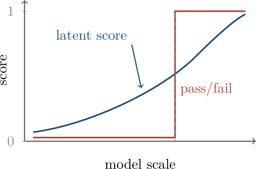
A useful way to summarize experiments is a phase diagram whose axes are regularization strength and data fraction. Delay is most visible when the rule exists, but memorization is initially easier. Too little data and weak regularization favor memorization. Enough data may make generalization easy. Appropriate regularization and enough signal make rule learning visible.
The same diagram should not be read as a universal law. For a different task, the axes might be model width and optimizer noise, or context length and training compute. What matters is the qualitative structure: some region makes memorization cheap, another makes the rule easy, and the grokking regime lies near a boundary where the optimizer first finds an interpolating solution and then slowly shifts to a structured one.
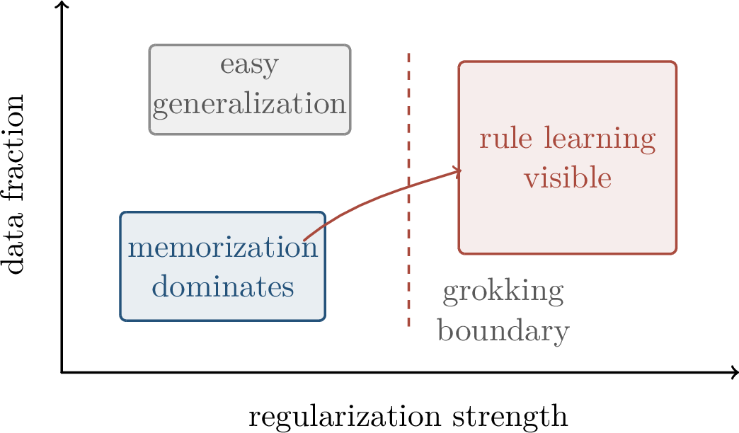
5.0.35 Measurement, Limits, and Open Questions↩︎
The right measurements include both external and internal quantities. External metrics include training and test loss, accuracy at multiple thresholds, calibration, margin, and robustness across random splits. Internal metrics include weight norms, effective rank, feature alignment with known structure, representation spectra, and causal circuit ablations. If accuracy is flat, one should look for continuous progress measures before concluding that learning has stopped.
A robust experimental protocol should therefore store full trajectories, not only final checkpoints. The most informative plots compare several clocks: training step, training loss, test loss, norm decay, margin growth, representation alignment, and causal circuit strength. A grokking claim is stronger when these clocks tell a coherent story: training fit appears first, hidden structure accumulates next, and test performance rises only after the structure is connected to the output.
There are also important limitations. Many grokking experiments use small algorithmic datasets, and transfer to large-scale natural data is subtle. Exact mechanisms depend on architecture, optimizer, regularization, and data split. Phase-transition language is qualitative unless a scaling limit and an order parameter are specified. Emergent-ability claims require care because sharp reported metrics do not by themselves prove sharp internal mechanisms.
Another limitation is that mechanistic explanations are usually task-specific. Finding a Fourier circuit for modular addition does not imply that the same model uses a similarly clean circuit for language, planning, or reasoning. The value of the toy setting is methodological: it teaches what to measure, how to separate memorization from rule learning, and how to test whether an apparent jump reflects hidden representation change.
Key open questions include: which inductive biases make algorithmic solutions easier to find; whether one can predict grokking delay from a task and architecture; when emergent abilities are genuine mechanism changes rather than threshold artifacts; and how to design benchmarks that reveal hidden progress rather than only final pass/fail behavior.
5.0.36 Summary↩︎
Grokking separates interpolation from generalization in time. The model can fit the training data long before it discovers a compact rule. Fourier analysis explains why modular addition has a compact solution, and mechanistic progress measures reveal hidden structure before visible test accuracy changes. Regularization and optimization select among many interpolating predictors, so late-time training dynamics matter. Finally, the connection to emergent abilities should be handled carefully: abrupt metrics may reflect genuine mechanisms, threshold artifacts, or a mixture of both.
Chapter Synthesis
Grokking is delayed generalization after interpolation: the model fits the training set early but generalizes only after a long plateau.
Modular arithmetic is a useful toy world because memorization and rule learning can both interpolate, while Fourier analysis gives an explicit compact rule.
Phase-transition language is meaningful only when paired with an order parameter that tracks an internal mechanism, not merely final accuracy.
Hidden progress measures, such as Fourier alignment or circuit scores, can improve smoothly before thresholded accuracy changes.
Weight decay, data fraction, architecture, and optimization dynamics influence whether training moves from a lookup-like solution to a shared rule.
Emergent abilities require careful measurement: an abrupt benchmark curve may reflect a new mechanism, a thresholded metric, or both.
Core sources include Power et al., Grokking: Generalization Beyond Overfitting on Small Algorithmic Datasets [23]; Nanda et al., Progress Measures for Grokking via Mechanistic Interpretability [58]; Liu et al., Omnigrok: Grokking Beyond Algorithmic Data; Barak et al., Hidden Progress in Deep Learning; Kumar et al., Grokking as the Transition from Lazy to Rich Training Dynamics; Wei et al., Emergent Abilities of Large Language Models [59]; Schaeffer et al., Are Emergent Abilities of Large Language Models a Mirage? [60]; and Wang et al., Grokked Transformers are Implicit Reasoners.
5.0.37 From Language Modeling to Preference Optimization↩︎
Pretraining teaches a language model to predict text. That objective is powerful because it extracts statistical structure from enormous corpora, but it is not the same as the objective we usually want at deployment time. A deployed assistant should answer helpfully, avoid misleading claims, refuse harmful requests, calibrate uncertainty, and respect the constraints of the interaction. These requirements are behavioral, contextual, and often difficult to encode as a single supervised target string.
The central idea in this chapter is to turn comparisons between possible model responses into an optimization objective. Instead of asking for a single gold response, we ask which of two responses is better for a prompt. The resulting label is a weak but flexible statement about behavior: \[y_{\mathrm{w}}\succ_x y_{\mathrm{l}},\] meaning that, for prompt \(x\), response \(y_{\mathrm{w}}\) is preferred to response \(y_{\mathrm{l}}\). Reinforcement learning from human feedback (RLHF) and direct preference optimization (DPO) are two mathematically connected ways to use such labels. RLHF was developed as a way to learn from human comparative feedback when hand-writing a reward function is difficult [24]; instruction-following language models popularized the pipeline of supervised fine-tuning followed by preference-based policy optimization [61]; DPO later showed that, under a KL-control model, one can optimize the policy directly from pairwise preferences without explicitly training and optimizing a separate reward model [62].
The preference viewpoint changes the unit of supervision. Next-token prediction treats the observed token as the target. Supervised fine-tuning treats a curated answer as the target. Preference optimization treats the ranking of candidate behaviors as the target. This is weaker than knowing the best possible response, but it is often more realistic: for open-ended questions there may be many acceptable answers, and a human rater can often say which answer is safer or more helpful without being able to write the ideal answer from scratch.
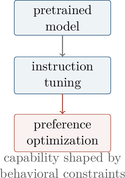
The first mathematical question is therefore:
How does a preference label become an objective for changing a language model policy?
The rest of the chapter answers this question in increasing detail. We first model preference data statistically. We then show that KL-regularized reward maximization has an explicit solution. Finally, we derive DPO by replacing the explicit reward model in the Bradley–Terry likelihood with the implicit reward defined by that solution.
Three distinctions will be useful throughout the chapter. First, a reward is a scalar modeling device; it is not the same thing as human values. Second, a reference policy is a behavioral prior that prevents optimization from moving too far away from the model that generated plausible language. Third, a preference objective is a proxy trained from finite comparisons; optimizing it can improve behavior, but it can also expose coverage gaps in the feedback data.
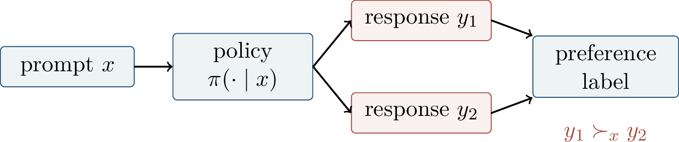
The word alignment is broader than the objectives in this chapter. Here it means the mathematical layer that converts feedback about desirable behavior into policy updates. This layer is only one part of safety: it does not by itself solve truthfulness, robustness, tool-use risk, long-horizon agency, or the social problem of whose preferences should be represented.
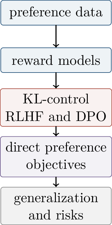
5.0.38 Preference Data and Reward Models↩︎
Definition 0.96 (Preference dataset). A pairwise preference dataset is a collection \[\mathcal{P}=\{(x_i,y_i^+,y_i^-)\}_{i=1}^n, \qquad y_i^+ \succ_{x_i} y_i^- .\] The prompt \(x_i\) is sampled from a prompt distribution, \(y_i^+\) is the preferred or chosen response, and \(y_i^-\) is the rejected response. In this chapter we also write \(y_{\mathrm{w}}=y^+\) and \(y_{\mathrm{l}}=y^-\).
Preference labels may come from human annotators, expert raters, AI feedback, or task verifiers. Their advantage is that comparisons are often easier and more reliable than scalar reward assignment. A rater may not know whether a response deserves reward \(7.3\) or \(8.1\), but may confidently choose the more accurate, concise, or safe response from a pair.
The construction of \(\mathcal{P}\) matters. The rejected response may be sampled from the same policy as the chosen response, from an earlier checkpoint, from a deliberately adversarial generator, or from a set of human-written alternatives. These choices determine which distinctions the reward model can learn. If all rejected responses are obviously bad, the data may teach coarse refusal or format preferences but not subtle truthfulness. If the pairs are too similar, labels may become noisy and expensive. Preference optimization begins as a statistical design problem before it becomes an optimization problem.
The classical statistical model for such data is the Bradley–Terry model. It assumes the existence of a latent reward or utility \(r^\star(x,y)\), but observes only noisy comparisons between reward differences.
Definition 0.97 (Bradley–Terry preference model). Given a latent reward \(r^\star:\mathcal{X}\times\mathcal{Y}\to\R\), the Bradley–Terry model sets \[\Prob(y_1\succ_x y_2) = \sigma\!\left(r^\star(x,y_1)-r^\star(x,y_2)\right), \qquad \sigma(t)=\frac{1}{1+e^{-t}}.\] Thus a large positive reward gap makes \(y_1\) very likely to be preferred, whereas equal rewards produce probability \(1/2\).
This model is deliberately minimal. It does not claim that human values are literally scalar or logistic. It gives a tractable likelihood for pairwise comparisons, and this likelihood is the bridge from labels to optimization.
The Bradley–Terry model should be read as a local approximation to a complex feedback process. The scalar reward represents whatever aspects of the response the annotator or feedback system is using on the sampled distribution. The sigmoid link says that only the reward difference matters, and that larger gaps make the preference more reliable. In real alignment datasets, labels also reflect ambiguity, fatigue, task instructions, rater expertise, and disagreement about values. The model is useful because it gives a simple loss, not because it captures every source of preference variation.
Definition 0.98 (Reward-model loss). For a parametric reward model \(\widehat r_\phi(x,y)\), define the score gap \[\Delta_\phi(x,y_{\mathrm{w}},y_{\mathrm{l}}) = \widehat r_\phi(x,y_{\mathrm{w}})-\widehat r_\phi(x,y_{\mathrm{l}}).\] The Bradley–Terry negative log-likelihood is \[\loss_{\mathrm{RM}}(\phi) = -\E_{(x,y_{\mathrm{w}},y_{\mathrm{l}})\sim\mathcal{P}} \log\sigma\!\left(\Delta_\phi(x,y_{\mathrm{w}},y_{\mathrm{l}})\right).\] Training a reward model is therefore logistic regression on reward differences.
Only differences of rewards are supervised. If \(\widehat r_\phi(x,y_{\mathrm{w}})\) and \(\widehat r_\phi(x,y_{\mathrm{l}})\) are both shifted upward by the same prompt-dependent constant, the comparison probability is unchanged. Likewise, the loss does not directly tell us whether a response is absolutely good; it tells us whether one response should score above another for the same prompt. This is why a reward model trained on comparisons must be evaluated by held-out pairwise accuracy, calibration, and downstream behavior rather than by interpreting its raw score as an absolute utility.
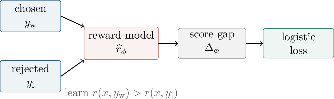
For any function \(c:\mathcal{X}\to\R\), the rewards \[r(x,y) \quadand\quad r'(x,y)=r(x,y)+c(x)\] induce exactly the same Bradley–Terry preference probabilities.
Proof. The likelihood depends only on within-prompt differences: \[r'(x,y_{\mathrm{w}})-r'(x,y_{\mathrm{l}}) = r(x,y_{\mathrm{w}})+c(x)-r(x,y_{\mathrm{l}})-c(x) = r(x,y_{\mathrm{w}})-r(x,y_{\mathrm{l}}).\] After applying the same sigmoid function, the pairwise preference probability is unchanged. ◻
This identifiability issue is more than a technicality. A reward model is a proxy trained from comparisons, not an absolute measurement device. Its zero level is arbitrary for each prompt, and even its extrapolation away from the labeled data is learned rather than observed. Later, when a policy is optimized against \(\widehat r_\phi\), these unobserved regions become important.
Example 0.19 (Why scalar rewards can mislead). Suppose two answers to a medical prompt are compared. The chosen answer is more cautious and cites uncertainty; the rejected answer is shorter but omits a critical caveat. A pairwise label says that the first answer is preferred. It does not uniquely determine how much the rater valued caution, how much they valued concision, or how the same rater would compare two longer answers. A reward model must infer a scalar explanation from many such comparisons. The inference can be useful, but it is underdetermined outside the coverage of the data.
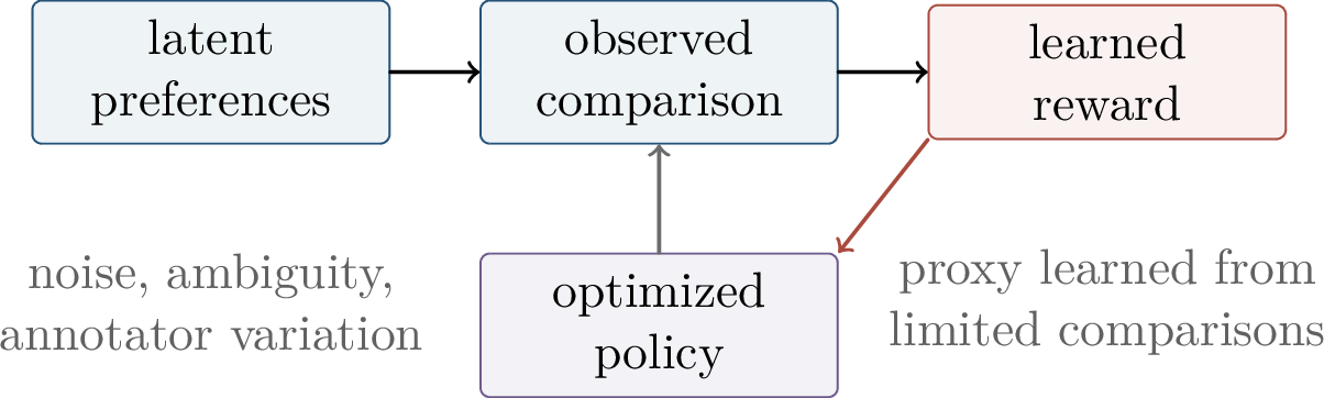
5.0.39 RLHF as KL-Regularized Control↩︎
In classical RLHF for language models, the reward model is used as an objective for policy optimization. The policy is not optimized freely: it is kept near a reference policy, usually the supervised fine-tuned model. This reference policy encodes fluency, instruction-following behavior, and a distributional prior over reasonable responses. In the language-model setting, this KL-regularized stage is the mathematical core of the RLHF pipeline used in instruction-following systems [61].
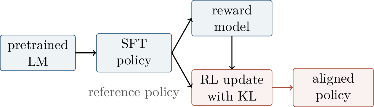
For a prompt \(x\), let \(\pi_{\mathrm{ref}}(\cdot\mid x)\) be the reference policy and let \(r(x,y)\) be a learned reward. The KL-regularized objective is \[J(\pi) = \E_{x\sim\mathcal{D},\;y\sim\pi(\cdot\mid x)} \left[ r(x,y) - \beta\log\frac{\pi(y\mid x)}{\pi_{\mathrm{ref}}(y\mid x)} \right],\] where \(\beta>0\). Equivalently, \[J(\pi) = \E_{x\sim\mathcal{D}} \left[ \E_{y\sim\pi(\cdot\mid x)} r(x,y) - \beta\,D_{\mathrm{KL}}\!\left(\pi(\cdot\mid x)\Vert \pi_{\mathrm{ref}}(\cdot\mid x)\right) \right].\] The parameter \(\beta\) prices movement away from the reference distribution. Large \(\beta\) penalizes drift strongly; small \(\beta\) permits more aggressive reward optimization.
The KL term has two roles. Statistically, it keeps the optimized policy near the region where the reward model was trained and where language quality is known to be reasonable. Algorithmically, it acts as a trust-region penalty: the policy may improve reward, but it must pay for increasing the probability of responses that the reference policy considered unlikely. Without such a penalty, reward maximization can collapse onto narrow, high-scoring responses that exploit reward-model errors.
Theorem 0.60 (KL-control solution). Fix a prompt \(x\), a reward function \(r(x,\cdot)\), and a reference policy \(\pi_{\mathrm{ref}}(\cdot\mid x)\) with support containing the support of the policies being optimized. The maximizer of \[\sum_y \pi(y\mid x)r(x,y) - \beta\sum_y \pi(y\mid x) \log\frac{\pi(y\mid x)}{\pi_{\mathrm{ref}}(y\mid x)}\] over distributions \(\pi(\cdot\mid x)\) is \[\pi_r(y\mid x) = \frac{1}{Z_r(x)} \pi_{\mathrm{ref}}(y\mid x)\exp\!\left(\frac{r(x,y)}{\beta}\right), \qquad Z_r(x)=\sum_{y'}\pi_{\mathrm{ref}}(y'\mid x) \exp\!\left(\frac{r(x,y')}{\beta}\right).\]
Proof. For a fixed \(x\), introduce a Lagrange multiplier \(\lambda\) for the normalization constraint \(\sum_y \pi(y\mid x)=1\). The Lagrangian is \[\mathcal{L}(\pi,\lambda) = \sum_y \pi(y\mid x)r(x,y) - \beta\sum_y \pi(y\mid x) \log\frac{\pi(y\mid x)}{\pi_{\mathrm{ref}}(y\mid x)} + \lambda\left(\sum_y\pi(y\mid x)-1\right).\] Stationarity with respect to \(\pi(y\mid x)\) gives \[r(x,y) - \beta\left( \log\frac{\pi(y\mid x)}{\pi_{\mathrm{ref}}(y\mid x)}+1 \right) + \lambda = 0.\] The terms \(-\beta+\lambda\) are constant in \(y\), so \[\log\frac{\pi(y\mid x)}{\pi_{\mathrm{ref}}(y\mid x)} = \frac{r(x,y)}{\beta} + C(x).\] Exponentiating and choosing the constant so that probabilities sum to one gives the stated Gibbs form. ◻
The theorem says that KL-regularized RL tilts the reference policy toward high-reward responses. It is not unconstrained maximization of \(r\). The reference distribution acts as a language prior and a trust region.
The support assumption is important. If \(\pi_{\mathrm{ref}}(y\mid x)=0\), then the KL penalty makes it impossible for an absolutely continuous policy to assign positive probability to \(y\). In neural language models, probabilities are usually nonzero on the token vocabulary, but sequence probabilities can still be astronomically small. The theorem should therefore be understood as an idealized finite-action calculation that explains the form of the objective, not as a prescription to enumerate all responses.
Two limiting cases build intuition. As \(\beta\to\infty\), the exponential tilt becomes weak and \(\pi_r(\cdot\mid x)\) stays close to \(\pi_{\mathrm{ref}}\). As \(\beta\to0\), the distribution concentrates on responses with maximal reward among those supported by the reference. Practical RLHF lives between these extremes: enough movement to improve behavior, but not so much that the reward proxy is optimized outside its reliable domain.
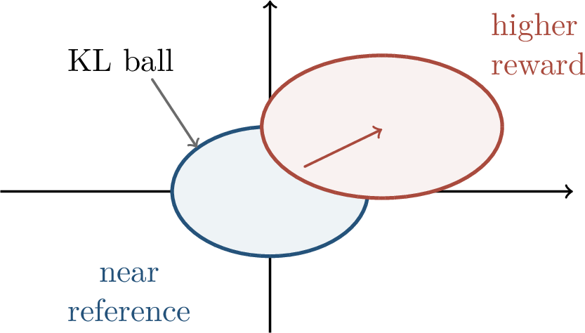
In large language models the exact maximizer is not computed by enumerating responses. Practical RLHF often uses a policy-gradient method such as PPO. The policy samples responses, receives a reward consisting of the learned reward model score plus a KL penalty, and updates iteratively. PPO-style clipping and explicit KL monitoring are meant to limit update size, but the procedure still has multiple moving parts: reward-model fitting, sampling, credit assignment, variance control, and policy optimization. DPO was motivated partly by the desire to replace this loop with a supervised-style objective that uses the same preference data.
This distinction is one reason the KL-control theorem is so useful pedagogically. It separates the population objective from the algorithm used to approximate it. PPO is one approximate optimizer for the KL-regularized reward objective. DPO is a different route: it uses the closed-form optimizer to eliminate the explicit reward and writes a supervised loss on policy log-probabilities. The two methods are connected by the same variational identity, even though their implementations look quite different.
5.0.40 DPO from the KL-Control Solution↩︎
The key observation behind DPO is that the KL-control theorem can be read in reverse. If a policy is optimal for some reward under the KL-regularized objective, then the reward can be expressed in terms of the policy and the reference. Rafailov et al. use this observation to derive a direct preference objective for language models [62].
Starting from \[\pi_r(y\mid x) = \frac{1}{Z_r(x)} \pi_{\mathrm{ref}}(y\mid x)\exp\!\left(\frac{r(x,y)}{\beta}\right),\] take logarithms and solve for \(r\): \[r(x,y) = \beta\log\frac{\pi_r(y\mid x)}{\pi_{\mathrm{ref}}(y\mid x)} + \beta\log Z_r(x).\] For pairwise comparisons at the same prompt, the normalizer cancels: \[r(x,y_{\mathrm{w}})-r(x,y_{\mathrm{l}}) = \beta\left[ \log\frac{\pi_r(y_{\mathrm{w}}\mid x)}{\pi_{\mathrm{ref}}(y_{\mathrm{w}}\mid x)} - \log\frac{\pi_r(y_{\mathrm{l}}\mid x)}{\pi_{\mathrm{ref}}(y_{\mathrm{l}}\mid x)} \right].\] DPO substitutes this implicit reward gap directly into the Bradley–Terry likelihood and parameterizes \(\pi_r\) by \(\pi_\theta\).
The cancellation of \(Z_r(x)\) is the algebraic reason DPO can avoid learning an explicit reward model. The normalizer depends on the prompt but not on the particular response within a same-prompt comparison. Since the Bradley–Terry likelihood uses only \(r(x,y_{\mathrm{w}})-r(x,y_{\mathrm{l}})\), the unknown prompt-dependent constant disappears. This is exactly the same invariance as in the prompt-shift proposition for reward models.
Definition 0.99 (Direct preference optimization). Given preference triples \((x,y_{\mathrm{w}},y_{\mathrm{l}})\), the DPO loss is \[\begin{align} \loss_{\mathrm{DPO}}(\theta) = -\E_{\mathcal{P}}\log\sigma\Big( \beta[ &\log\pi_\theta(y_{\mathrm{w}}\mid x)-\log\pi_{\mathrm{ref}}(y_{\mathrm{w}}\mid x)\\ &-\log\pi_\theta(y_{\mathrm{l}}\mid x)+\log\pi_{\mathrm{ref}}(y_{\mathrm{l}}\mid x)] \Big). \end{align}\] Equivalently, with \[m_\theta(x,y_{\mathrm{w}},y_{\mathrm{l}}) = \log\frac{\pi_\theta(y_{\mathrm{w}}\mid x)}{\pi_\theta(y_{\mathrm{l}}\mid x)} - \log\frac{\pi_{\mathrm{ref}}(y_{\mathrm{w}}\mid x)}{\pi_{\mathrm{ref}}(y_{\mathrm{l}}\mid x)},\] the loss is \(-\E_{\mathcal{P}}\log\sigma(\beta m_\theta)\).
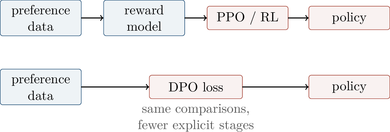
DPO increases the policy log-odds of the preferred response relative to the reference policy. Its comparison statistic is \[m_\theta = \log\frac{\pi_\theta(y_{\mathrm{w}}\mid x)}{\pi_\theta(y_{\mathrm{l}}\mid x)} - \log\frac{\pi_{\mathrm{ref}}(y_{\mathrm{w}}\mid x)}{\pi_{\mathrm{ref}}(y_{\mathrm{l}}\mid x)}.\] Thus the loss does not merely ask whether \(\pi_\theta\) assigns higher probability to \(y_{\mathrm{w}}\) than to \(y_{\mathrm{l}}\); it asks whether \(\pi_\theta\) improves that odds ratio beyond what the reference already believed.
Proof. Collect the four log-probability terms in the DPO logit: \[\log\pi_\theta(y_{\mathrm{w}}\mid x)-\log\pi_\theta(y_{\mathrm{l}}\mid x) - \log\pi_{\mathrm{ref}}(y_{\mathrm{w}}\mid x)+\log\pi_{\mathrm{ref}}(y_{\mathrm{l}}\mid x).\] This is exactly the difference between the new policy log-odds and the reference policy log-odds. ◻
The reference term is essential. Without it, a preference loss could reward responses that were already likely under the base model rather than responses made more preferred by alignment. With the reference correction, DPO learns how the aligned policy should deviate from the starting policy.
The margin \(m_\theta\) is therefore a change in relative odds. If the reference already strongly prefers \(y_{\mathrm{w}}\) over \(y_{\mathrm{l}}\), then the optimized policy does not need to create that preference from scratch. If the reference prefers \(y_{\mathrm{l}}\), then DPO must overcome the reference odds. This makes the objective conservative in a precise sense: it measures alignment progress relative to the behavior already encoded in \(\pi_{\mathrm{ref}}\).
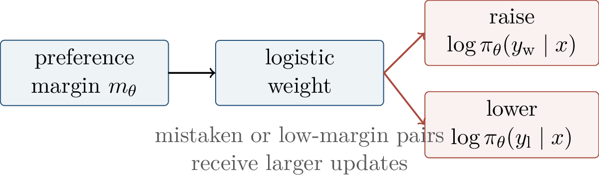
To see this analytically, write the loss on one example as \[\ell_\theta=-\log\sigma(\beta m_\theta).\] Then \[\nabla_\theta \ell_\theta = -\beta\bigl(1-\sigma(\beta m_\theta)\bigr) \nabla_\theta m_\theta .\] Gradient descent therefore increases \(m_\theta\). If the winner already has a large positive margin, the multiplier \(1-\sigma(\beta m_\theta)\) is small. If the current policy under-ranks the winner, the multiplier is large.
Expanding \(\nabla_\theta m_\theta\) shows the contrastive form: \[\nabla_\theta m_\theta = \nabla_\theta\log\pi_\theta(y_{\mathrm{w}}\mid x) - \nabla_\theta\log\pi_\theta(y_{\mathrm{l}}\mid x),\] because the reference terms are fixed. Thus a DPO update increases the log-likelihood of the chosen response and decreases the log-likelihood of the rejected response, with a strength determined by the current margin. The loss looks supervised, but it is not ordinary supervised fine-tuning: the rejected response and the reference correction are part of the signal.
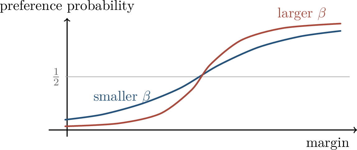
In the KL-control objective, \(\beta\) is the coefficient on the KL penalty. In the DPO loss, the same symbol scales the reference-corrected margin. This is not an accident: DPO inherits \(\beta\) from the Gibbs-form solution. In practice it is tuned as a stability and alignment-strength parameter.
Small \(\beta\) makes the logistic logit less sensitive to margin differences, so updates remain active over a wider range of examples. Large \(\beta\) turns modest margin differences into confident preference probabilities, which can make updates sharper but also more sensitive to noisy labels. The best value is therefore empirical: it depends on the quality of the preference data, the strength of the reference model, and how far the policy should move.
5.0.41 The Preference-Optimization Family↩︎
DPO is one point in a larger design space. Many methods optimize a surrogate loss on a policy-dependent score difference: \[\E_{(x,y_{\mathrm{w}},y_{\mathrm{l}})\sim\mathcal{P}} \Phi\!\left( s_\theta(x,y_{\mathrm{w}})-s_\theta(x,y_{\mathrm{l}}) \right),\] where \(s_\theta\) is often a log probability, a reference-corrected log ratio, or a margin-shifted variant, and \(\Phi\) is a decreasing loss. Different methods change the feedback format, the reference term, the target margin, or the way preference learning is combined with supervised fine-tuning.
This template clarifies what is shared across the family. Each method defines a score that should be higher for desirable behavior than for undesirable behavior, and each method chooses how strongly to penalize deviations from a base model. The differences are not cosmetic: removing a reference changes the implicit regularization; replacing a logistic loss by a finite-margin loss changes what happens on separable data; using binary feedback instead of pairs changes which comparisons are observed.
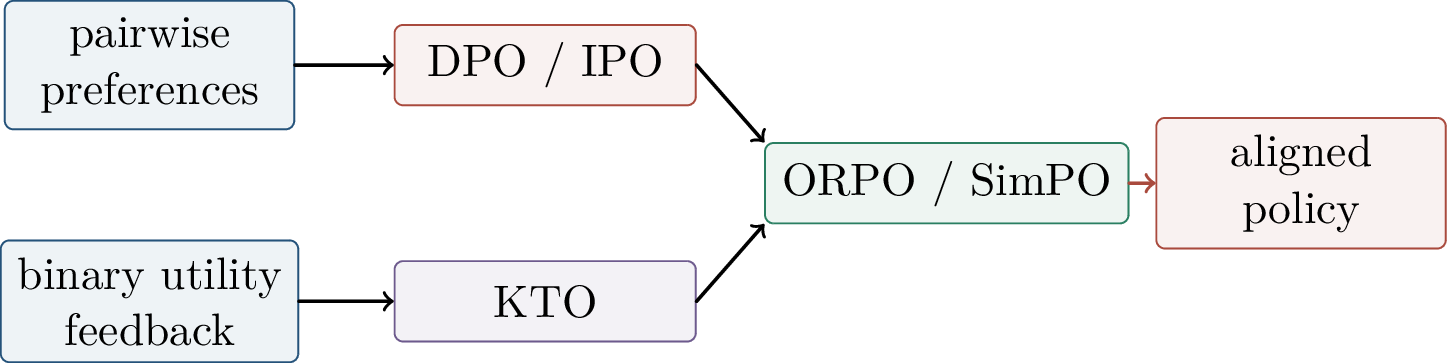
5.0.41.0.0.1 IPO and margins.
The logistic DPO loss can continue increasing preference margins when labels are nearly separable. IPO-style views introduce a finite target scale. A simplified margin loss has the form \[\left( \log\frac{\pi_\theta(y_{\mathrm{w}}\mid x)}{\pi_{\mathrm{ref}}(y_{\mathrm{w}}\mid x)} - \log\frac{\pi_\theta(y_{\mathrm{l}}\mid x)}{\pi_{\mathrm{ref}}(y_{\mathrm{l}}\mid x)} - m \right)^2,\] where \(m>0\) is a desired margin. The purpose is not merely to make the winner more likely forever, but to reach an appropriate preference separation.
5.0.41.0.0.2 KTO without explicit pairs.
Kahneman–Tversky Optimization (KTO) is designed for feedback of the form \[(x,y,z),\qquad z\in\{+1,-1\},\] where \(z=+1\) marks desirable behavior and \(z=-1\) marks undesirable behavior. The objective applies asymmetric gains and losses to policy log-ratios, inspired by prospect theory. This is useful when pairwise comparisons are unavailable but thumbs-up and thumbs-down style labels exist.
5.0.41.0.0.3 ORPO and SimPO.
ORPO and SimPO simplify direct preference training. ORPO combines supervised fine-tuning with an odds-ratio preference penalty, avoiding a separate reference model in the optimization objective. SimPO uses the policy’s own length-normalized likelihood as a reference-free reward and adds a target margin. These variants trade some theoretical closeness to the original KL-control derivation for implementation simplicity and empirical stability.
| Method | Signal | Main idea |
|---|---|---|
| RLHF | pairs plus reward model | learn a scalar reward, then optimize it with a KL penalty to a reference policy |
| DPO | chosen versus rejected | optimize logistic preference likelihood on reference-corrected policy log-ratios |
| IPO | chosen versus rejected | use a finite target margin to avoid unbounded preference pushing |
| KTO | desirable or undesirable labels | use asymmetric utility on policy log-ratios when explicit pairs are absent |
| ORPO / SimPO | pairs | simplify the objective by modifying or removing the explicit reference term |
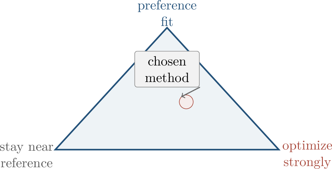
This family perspective is useful when comparing algorithms. The question is not whether one loss is universally correct. The question is which assumptions are appropriate: pairwise labels or binary labels, a trusted reference or reference-free scoring, a logistic likelihood or finite margin, and a separate reward model or a direct loss.
There is also an optimization tradeoff. RLHF exposes the reward model and can use on-policy samples during policy optimization, but it introduces the instability and variance of reinforcement learning. DPO is simpler and supervised-style, but it trains only on the comparison distribution unless new pairs are collected. Reference-free objectives simplify implementation, but they must replace the stabilizing role that the reference policy played in the KL-control derivation.
5.0.42 Generalization and Failure Modes↩︎
Preference optimization introduces a second layer of generalization. The base model must generalize from pretraining and supervised data, and the preference model or preference objective must generalize from the comparison dataset to the responses produced by the optimized policy. The latter distribution is not fixed: the more strongly we optimize, the more the policy may visit responses unlike the ones that were labeled.
This is the alignment analogue of covariate shift. The feedback data are collected under one response distribution, but the optimized policy defines a new distribution. If the new policy discovers response styles, lengths, formats, or loopholes that were rare in the data, the reward model or direct preference objective may be forced to extrapolate. The KL penalty, reference terms, iterative data collection, and adversarial evaluation are all attempts to control this moving-target problem.
Definition 0.100 (Reward-model generalization gap). Let \(\pi_{\mathrm{train}}\) denote the distribution that generated the comparison data, and let \(\pi_\theta\) be the optimized policy. A reward-model generalization gap is the mismatch between preference prediction quality under the training distribution and under the optimized policy distribution: \[\E_{\pi_{\mathrm{train}}} \ell_{\mathrm{pref}}(\widehat r) \quadversus\quad \E_{\pi_\theta} \ell_{\mathrm{pref}}(\widehat r).\] If \(\pi_\theta\) moves into regions where labels are scarce, the learned reward may extrapolate incorrectly.
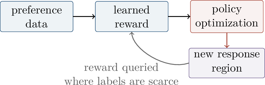
5.0.42.0.0.1 Reward hacking.
Reward hacking occurs when a policy finds responses that score highly under the proxy reward while failing the intended objective. In language models, this may appear as verbosity that pleases a reward model, confident but false answers, superficial refusal patterns, or artifacts that exploit an automated judge. The mathematical pattern is simple: optimizing an imperfect proxy can amplify the proxy’s errors.
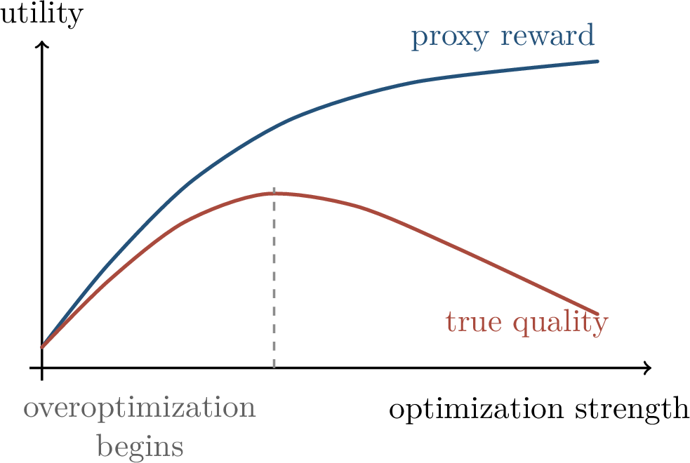
Goodhart’s law is not a theorem about every reward model, but it is a useful warning. If a proxy is selected because it correlates with quality on the training distribution, strong optimization can select examples where the correlation breaks.
Example 0.20 (Verbosity as a proxy). Suppose annotators often prefer detailed answers to terse answers because the terse answers omit important qualifications. A reward model may learn that length is a useful predictor of preference. During optimization, the policy can then produce unnecessarily long answers that score well under the proxy while becoming less useful to the user. The problem is not that detail is bad; the problem is that a correlation in the comparison data has been promoted into an optimization target.
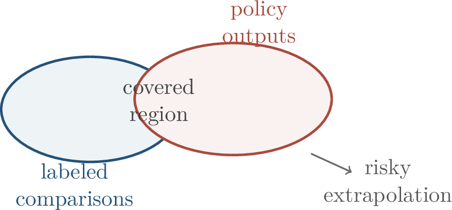
5.0.42.0.0.2 Preference ambiguity.
Human preferences are not a single deterministic function. They differ across annotators, cultures, expertise levels, and available context. Pairwise labels may be inconsistent, and a majority label may hide serious minority harms. A scalar reward is especially crude when a task has multiple valid tradeoffs, such as being concise versus being complete, or being helpful versus refusing unsafe assistance. In such settings, calibrated uncertainty, plural preference models, and explicit constraints may be more appropriate than pretending that every disagreement is just logistic noise.
Preference ambiguity also affects evaluation. A high held-out preference accuracy can coexist with systematic failure on a subgroup of prompts or for a minority rater population. When disagreement is meaningful, averaging labels can erase the structure one most needs to preserve. Alignment experiments should therefore inspect disagreement, not merely treat it as label noise.
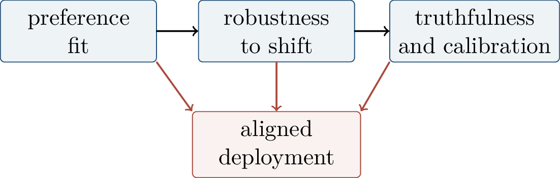
During training, monitor KL to the reference, chosen and rejected log-likelihoods, held-out preference accuracy, reward-model calibration, and examples with extreme reward. During evaluation, test adversarial prompts, distribution shifts, refusal quality, truthfulness, calibration, and disagreement between human and automated judges. A high preference score is evidence, not a guarantee.
5.0.43 What the Theory Explains and What It Leaves Open↩︎
The theory in this chapter explains several central facts cleanly. Pairwise preferences can be modeled by a Bradley–Terry likelihood. KL-regularized reward maximization has an explicit Gibbs-form optimizer. DPO follows by substituting the implicit reward from that optimizer into the preference likelihood. The reference policy and temperature are not arbitrary details: they control how policy movement is measured and scaled.
At the same time, many questions are not settled by the derivation. The Bradley–Terry model does not solve preference aggregation. KL control does not guarantee safety under distribution shift. Direct objectives do not eliminate the possibility of overoptimization; they change where the proxy appears. Open-ended language models also raise questions about long-horizon tool use, multi-agent effects, scalable oversight, and values that are contextual or plural.
This is the main conceptual lesson of the chapter. The mathematics explains a clean conversion from pairwise feedback to policy updates, but it does not make the feedback complete, representative, or value-correct. Preference optimization is a powerful interface between human judgments and model behavior. It should be paired with uncertainty estimates, coverage analysis, red-teaming, task-specific constraints, and post-training evaluation that is not reducible to the training preference objective.
5.0.44 Summary↩︎
RLHF and DPO are two views of the same preference-to-policy problem. RLHF learns a reward model from pairwise comparisons and optimizes it while penalizing KL divergence from a reference policy. The KL-regularized objective has a Gibbs-form solution: the optimized policy is the reference policy tilted by exponentiated reward. DPO reverses this solution, writes an implicit reward in terms of policy log-ratios, and places that reward difference inside the Bradley–Terry preference likelihood. This yields a direct supervised-style loss on chosen and rejected responses.
The derivation is elegant, but the limitations are just as important. Reward models and direct preference losses are trained on finite, noisy, and ambiguous feedback. Strong optimization can shift the policy into regions where the proxy is poorly constrained. Alignment therefore requires not only preference fitting, but also coverage, robustness, calibration, uncertainty, and careful evaluation.
Chapter Synthesis
Preference optimization replaces single target responses by comparisons between candidate behaviors, making it suitable for open-ended assistance.
Bradley–Terry reward modeling converts pairwise labels into logistic regression on reward differences, but rewards are identifiable only up to prompt-dependent shifts.
KL-regularized reward maximization has a Gibbs-form solution: the optimized policy is the reference policy tilted by exponentiated reward.
DPO substitutes the implicit KL-control reward into the Bradley–Terry likelihood, producing a supervised-style loss on reference-corrected policy log-ratios.
The reference policy and temperature parameter control how far and how sharply the policy moves away from its starting behavior.
Generalization is the central risk: reward models and direct objectives can be optimized outside the coverage of the preference data, leading to reward hacking or Goodhart effects.
Core sources include Christiano et al., Deep Reinforcement Learning from Human Preferences [24]; Ziegler et al., Fine-Tuning Language Models from Human Preferences; Stiennon et al., Learning to Summarize with Human Feedback; Ouyang et al., Training Language Models to Follow Instructions with Human Feedback [61]; Bai et al., Constitutional AI: Harmlessness from AI Feedback; Rafailov et al., Direct Preference Optimization: Your Language Model is Secretly a Reward Model [62]; Azar et al., A General Theoretical Paradigm to Understand Learning from Human Preferences; Ethayarajh et al., KTO: Model Alignment as Prospect Theoretic Optimization; Hong et al., ORPO: Monolithic Preference Optimization without Reference Model; Meng et al., SimPO: Simple Preference Optimization with a Reference-Free Reward; and Schulman et al., Proximal Policy Optimization Algorithms.
5.0.45 Why OOD Theory Is a Deployment Theory↩︎
The standard supervised-learning story assumes a contract: training and test examples are drawn from the same distribution. Earlier chapters used this contract when bounding generalization gaps, studying implicit regularization, and analyzing the behavior of large models. Deployment often breaks it. A medical model moves from one hospital to another; a vision system sees a new camera and climate; a language model meets new laws, prompt styles, APIs, tools, users, and reward models. The model may still be solving the same task, but the distribution has changed.
Foundation models sharpen the question rather than removing it. Broad pretraining exposes a model to many data sources and often improves transfer, but deployment still asks for behavior under a target distribution that was not exactly the training mixture. Thus the central question of this chapter is:
When does low training-domain risk imply low risk on a new distribution?
The answer is never “always.” OOD generalization is possible only under a relation between the observed environments and the deployment environment. Sometimes this relation is statistical, as in covariate shift or domain adaptation. Sometimes it is structural, as in the assumption that a causal mechanism remains invariant while nuisance variables change. Sometimes it is operational: a model may detect that an input is unfamiliar and route it to a human or a safer fallback. The purpose of OOD theory is to make these assumptions explicit, not to promise distribution-free extrapolation.
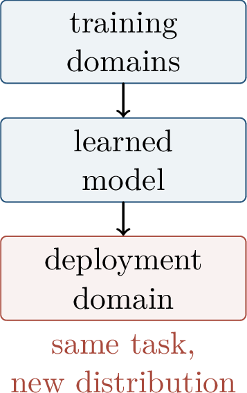
The distribution shift creates an extra term beyond ordinary finite-sample generalization. If \(P\) is the training distribution and \(Q\) is the deployment distribution, then \[\mathcal{R}_Q(f) = \mathcal{R}_P(f)+\Delta_{P\to Q}(f),\] where \(\Delta_{P\to Q}(f)\) denotes the price of changing distributions. Classical generalization theory controls the difference between empirical and population risk under \(P\). OOD theory asks what can be said about \(\Delta_{P\to Q}(f)\), and under what assumptions it can be small.
This extra term is why OOD risk is a deployment quantity rather than a purely training-time quantity. If \(Q=P\), then standard generalization and optimization analyses may be enough. If \(Q\neq P\), then even a predictor with tiny source risk may fail for one of three reasons: the target inputs may lie in a region not covered by the source, the target labels may follow a different rule, or the learned representation may rely on a shortcut that was predictive only in the source domain.
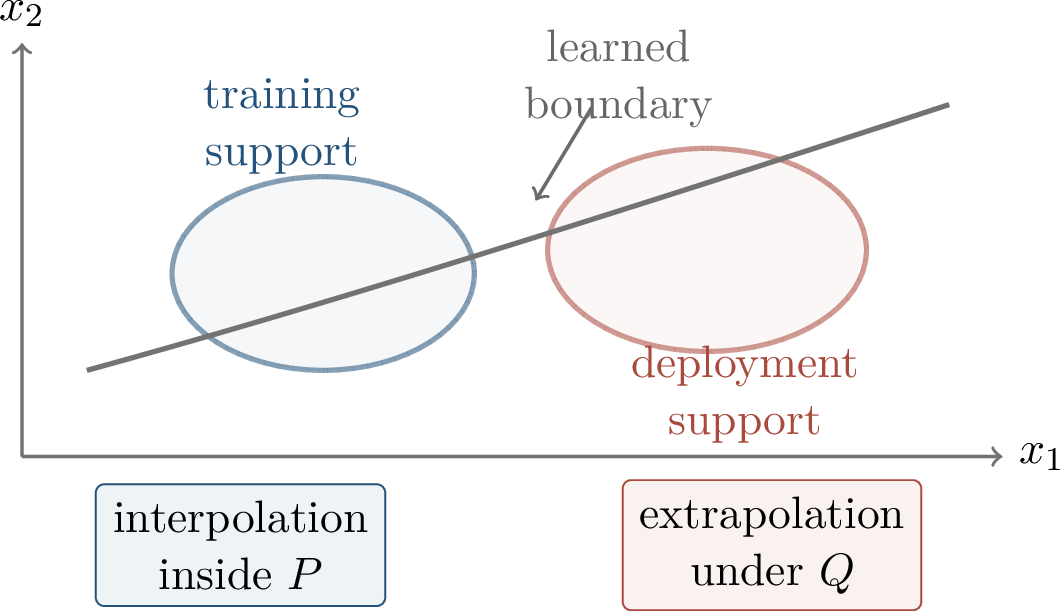
There are several common names for recurring shift patterns. Under covariate shift, \(P(X)\neq Q(X)\) but \(P(Y\mid X)\) is stable. Under label shift, \(P(Y)\neq Q(Y)\) but \(P(X\mid Y)\) is stable. Under concept shift, the conditional rule \(P(Y\mid X)\) itself changes. Subpopulation shift changes the mixture weights among groups, while semantic shift changes a latent nuisance, instruction, or mechanism that may not be cleanly visible in the input variables. These names are diagnostic language, not guarantees. A method succeeds only when the shift model is connected to an assumption that is testable, plausible, or enforced by data collection.
The most common mistake is to name the shift without checking whether the corresponding stable part is believable. Covariate shift is useful only if \(P(Y\mid X)\) is really stable; label shift is useful only if class-conditional features are stable; invariance methods need environments that vary the spurious factors while preserving the core mechanism. Thus data collection is part of the theorem: the environments must contain the right variation for the learning algorithm to distinguish stable from unstable predictors.
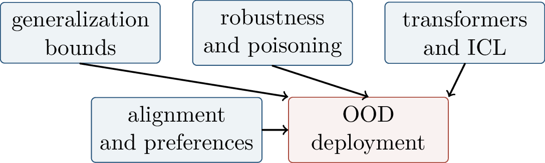
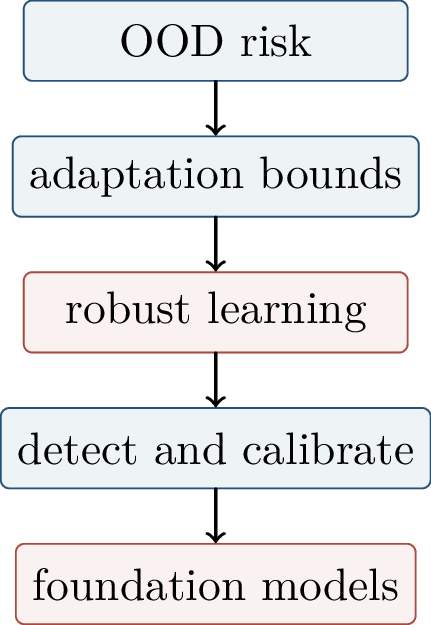
5.0.46 Environments, Risks, and Shift Models↩︎
Definition 0.101 (Environment model and OOD risk). Let \(e\in\mathcal{E}\) index a distribution \(P_e\) on \(\mathcal{X}\times\mathcal{Y}\). For a predictor \(f:\mathcal{X}\to\mathcal{Y}\), define \[\mathcal{R}_e(f) = \E_{(X,Y)\sim P_e}\big[\ell(f(X),Y)\big].\] If \(\mathcal{E}_{\mathrm{train}}\) is the set of observed environments and \(\mathcal{E}_{\mathrm{test}}\) is a set of unseen deployment environments, an OOD objective is to control \[\mathcal{R}_{\mathrm{OOD}}(f) = \sup_{e\in\mathcal{E}_{\mathrm{test}}}\mathcal{R}_e(f), \qquad \mathcal{E}_{\mathrm{test}}\not\subseteq \mathcal{E}_{\mathrm{train}}.\]
This formulation emphasizes that OOD generalization is not a single problem. The theorem one can prove depends on how the test environments are related to the observed ones. Three protocols are especially common.
The supremum in \(\mathcal{R}_{\mathrm{OOD}}(f)\) should also be interpreted with care. If \(\mathcal{E}_{\mathrm{test}}\) is too large, the objective is impossible: it includes environments with arbitrary labels. If \(\mathcal{E}_{\mathrm{test}}\) is too narrow, the objective may miss the shift that matters in deployment. The modeling work is therefore to specify a family of plausible target environments. In applied settings this family may be determined by hospitals, geographies, time periods, user groups, prompt templates, or known nuisance variables.
Definition 0.102 (Three OOD protocols). In domain adaptation, a source distribution \(P_{\mathrm{src}}\) and a target distribution \(P_{\mathrm{tgt}}\) differ, and unlabeled or weakly labeled target samples are often available. In domain generalization, several source environments \(P_1,\ldots,P_m\) are available but the target domain is unseen until deployment. In OOD detection, the task is to decide whether an input is drawn from an in-distribution law \(P_{\mathrm{ID}}\) or from an OOD law before making, abstaining from, or routing a prediction.
The protocols differ in what information is available at training or adaptation time. Domain adaptation may use unlabeled target inputs, so it can measure how target covariates differ from source covariates. Domain generalization has no such target sample, so it must infer stable structure from multiple observed environments. OOD detection is not asked to predict correctly everywhere; it is asked to decide when the ordinary predictor should not be trusted.
| Shift | Stable part | Changed part |
|---|---|---|
| Covariate shift | \(P(Y\mid X)\) | \(P(X)\) |
| Label shift | \(P(X\mid Y)\) | \(P(Y)\) |
| Concept shift | none required | \(P(Y\mid X)\) |
| Subpopulation shift | task rule | group mixture |
| Semantic shift | latent task | nuisance mechanism |
Example 0.21 (Spurious correlation toy model). Let \[X=(X_{\rm core},X_{\rm spur}),\qquad Y\in\{-1,1\},\] and suppose that the stable rule is \[Y=\sign(X_{\rm core})\] in every environment. The spurious feature, however, has environment-dependent correlation \[\Prob_e(X_{\rm spur}=Y)=p_e.\] If \(p_e\) is large in training environments, ERM may prefer \(X_{\rm spur}\) because it is easier to exploit. At deployment, a change in \(p_e\) can reverse the apparent rule.
This toy model is deliberately simple, but it captures a common failure mode. The shortcut \(X_{\rm spur}\) is not useless: in the source environments it may be more predictive than the core feature and may be easier for a neural network to learn. The problem is that its predictive relation is environment-specific. If all training environments have the same shortcut correlation, the data do not reveal that the feature is unstable. If environments vary \(p_e\), then robust or invariant objectives have a chance to identify \(X_{\rm core}\) as the feature whose relation to \(Y\) persists.
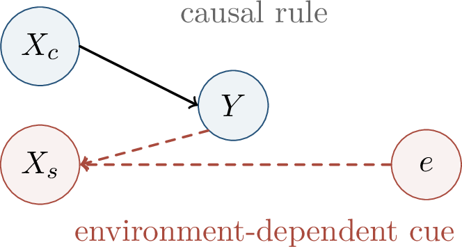
The example exposes the necessary ingredients for OOD learning. The target should not require unconstrained prediction on a region with no source information; some conditional, representation, or mechanism must be shared; the training environments must vary enough to reveal unstable cues; and the learning rule must prefer the stable structure over shortcuts.
Without assumptions on the relation between \(Q\) and \(P\), a predictor can be perfect on all source observations and arbitrary on the target support. OOD theory is therefore not a search for a universal shift-proof algorithm. It is a way to state, test, and exploit assumptions about the shift.
5.0.47 Adaptation Bounds and Impossibility↩︎
The cleanest mathematical entry point is the domain adaptation bound of Ben-David and collaborators. It separates target error into three pieces: source error, a distributional discrepancy, and an irreducible term measuring whether one classifier can serve both domains [63].
Definition 0.103 (\(\mathcal{H}\Delta\mathcal{H}\) divergence). For a binary hypothesis class \(\mathcal{H}\), define \[d_{\mathcal{H}\Delta\mathcal{H}}(P,Q) = 2\sup_{h,h'\in\mathcal{H}} \left| \Prob_{P}\!\big[h(X)\neq h'(X)\big] - \Prob_{Q}\!\big[h(X)\neq h'(X)\big] \right|.\] This divergence measures how differently hypotheses in \(\mathcal{H}\) can disagree on the two marginal input distributions.
The definition is tailored to classification. It does not ask whether \(P_X\) and \(Q_X\) are close in total variation over all measurable sets. It asks whether the particular hypothesis class can witness a difference through disagreement regions \(\{x:h(x)\neq h'(x)\}\). If no pair of hypotheses in \(\mathcal{H}\) can distinguish the domains by their disagreement behavior, the discrepancy term is small for that class. This is why representation learning can help: after mapping \(X\) to \(\Phi(X)\), the domains may become less distinguishable by the downstream hypothesis class.
Theorem 0.61 (Ben-David et al. domain adaptation bound). For binary classification and \(h\in\mathcal{H}\), \[\epsilon_T(h) \le \epsilon_S(h) +\frac{1}{2}d_{\mathcal{H}\Delta\mathcal{H}}(P_X^S,P_X^T) +\lambda^*,\] where \[\lambda^* = \min_{h\in\mathcal{H}}\big(\epsilon_S(h)+\epsilon_T(h)\big).\]
The three terms have distinct meanings. A high source error means that ordinary training failed. A high \(\mathcal{H}\Delta\mathcal{H}\) discrepancy means that the source and target feature distributions remain distinguishable by the hypothesis class. A high \(\lambda^*\) means that no classifier in the class is simultaneously good on both domains; this is a concept-shift or shared-rule failure rather than merely a representation-alignment failure.
The proof idea is a triangle inequality around the best joint classifier \(h^*\). For target error, compare \(h\) to \(h^*\) on the target domain, replace the resulting disagreement by source disagreement plus an \(\mathcal{H}\Delta\mathcal{H}\) discrepancy term, and then add the source error of \(h^*\) and the target error of \(h^*\). The last two terms form \(\lambda^*\). The bound is therefore not a magic transfer theorem: if the best shared classifier is bad, no amount of marginal alignment can make the target error small.
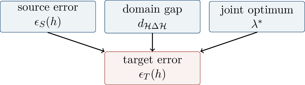
The operational interpretation of the discrepancy term leads to domain-adversarial learning. If a domain classifier can easily distinguish source from target in a learned representation \(\Phi(X)\), then the discrepancy is large and the target bound is loose. A domain-adversarial network therefore trains features that are useful for the task while hiding domain identity.
This logic also explains a limitation. Removing all domain information is not always desirable. Domain identity may contain label-relevant information, or two domains may require different decision rules. Domain-adversarial learning is appropriate when there exists a representation that preserves label information while discarding nuisance domain information. If this assumption is false, adversarial alignment can reduce the discrepancy term while increasing \(\lambda^*\).
Definition 0.104 (Domain-adversarial template). Let \(g\) be a task predictor, \(a\) a domain predictor, and \(\Phi\) a representation. A stylized objective is \[\min_{\Phi,g}\max_a \mathcal{R}_{\rm task}(g\circ\Phi) - \gamma\,\mathcal{R}_{\rm domain}(a\circ\Phi).\] The maximization over \(a\) tries to classify the domain, while the minimization over \(\Phi\) tries to make that classification difficult without destroying task information.
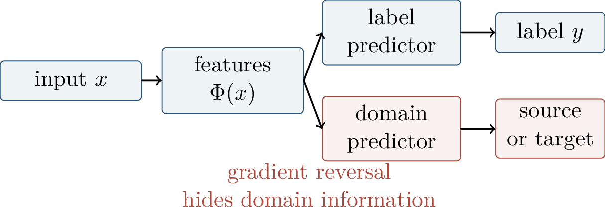
The adaptation bound also points to an impossibility: making marginals look similar cannot create labels where there is no source information.
Suppose there is a set \(A\subseteq\mathcal{X}\) such that \[P_X(A)=0,\qquad Q_X(A)>0.\] If target labels on \(A\) are unconstrained, then two target problems can agree on all source observations and disagree on \(A\). Therefore no source-only learner can guarantee low target error for both target problems.
Proof. Because \(P_X(A)=0\), source data carry no information about labels on \(A\). Construct two target label rules that coincide outside \(A\) and are opposite on \(A\). They induce identical source observations but require different predictions on a set of positive \(Q_X\)-mass. Any source-only algorithm must output the same predictor for the two indistinguishable source problems, so it is wrong on \(A\) for at least one of them. ◻
One recent response is testable learning with distribution shift: the learner receives labeled source data and unlabeled target data and must either output a low-risk predictor or reject the target sample. The goal is not to assume that every shift is benign, but to make the guarantee falsifiable by a discrepancy test tied to the hypothesis class.
5.0.48 Robust and Invariant Training↩︎
When multiple source environments or group labels are available, the training objective can be changed to reflect the desired deployment behavior. Average training risk is not always the right target.
The key modeling choice is what the observed environments mean. If they are subpopulations that may be reweighted at deployment, a worst-group objective is natural. If they are interventions that change nuisance correlations while preserving a causal rule, an invariance objective is natural. If they are arbitrary dataset partitions with no relation to the deployment shift, robust objectives may simply optimize the wrong notion of robustness.
Definition 0.105 (ERM and group DRO). Empirical risk minimization over environments optimizes the average risk, \[\min_f \frac{1}{m}\sum_{e\in\mathcal{E}_{\mathrm{train}}}\mathcal{R}_e(f).\] Group distributionally robust optimization instead optimizes the worst observed environment, \[\min_f \max_{e\in\mathcal{E}_{\mathrm{train}}}\mathcal{R}_e(f).\]
Group DRO is motivated by subpopulation and group shifts. If a deployment distribution resembles a mixture or perturbation of observed groups, then minimizing the worst observed group risk is closer to deployment risk than minimizing only the average. It prevents a large or easy group from hiding a small but important failure mode.
The price is that group labels and group coverage are needed. If the difficult group is absent from training, group DRO cannot protect it. If groups are defined too coarsely, the worst-group loss may still hide failures inside a group. If groups are too small, empirical estimates of group risk can be noisy and overfit. Thus group DRO is a method for observed group shift, not a universal OOD guarantee.
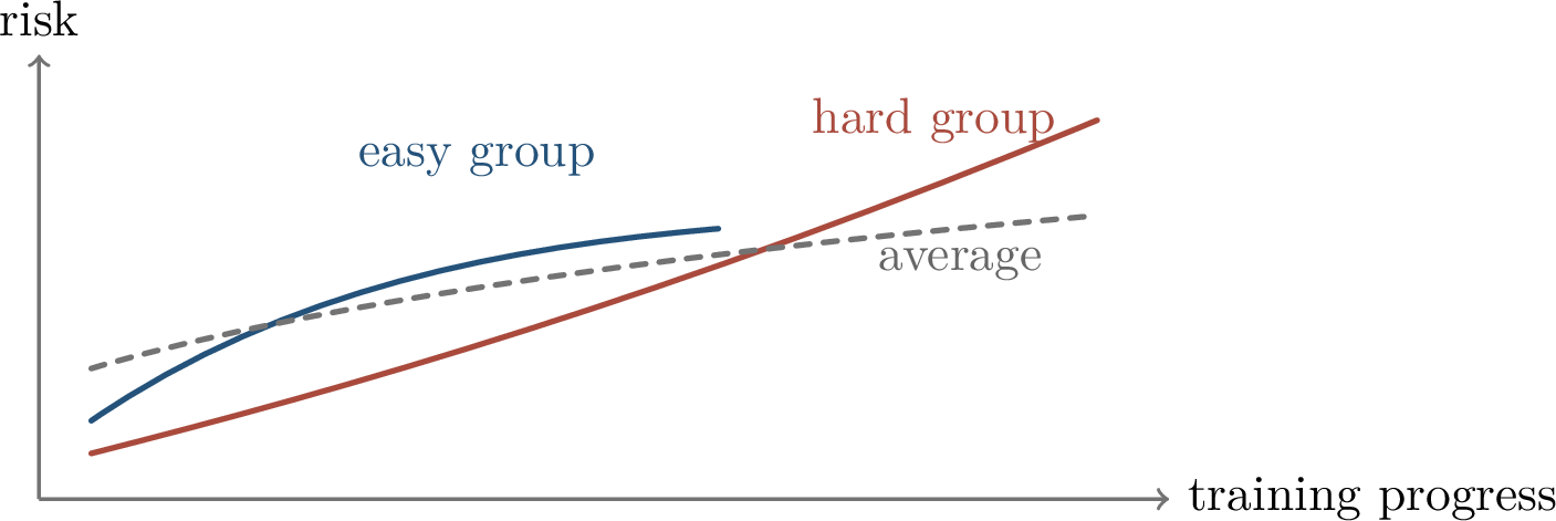
Definition 0.106 (Invariant Risk Minimization). The ideal IRM objective seeks a representation \(\Phi\) such that the same classifier \(w\) is optimal in every training environment: \[\min_{\Phi,w} \sum_{e\in\mathcal{E}_{\mathrm{train}}}\mathcal{R}_e(w\circ\Phi) \quad s.t.\quad w\in\argmin_{\bar w}\mathcal{R}_e(\bar w\circ\Phi) \quad \forall e.\]
The intuition is that stable predictors should remain optimal when nuisance correlations change across environments. If shape is causally related to an object label but background is only spuriously correlated, then changing the background-label correlation across environments can reveal the stable feature.
IRM differs from group DRO in its target. Group DRO asks for uniformly low risk on observed groups. IRM asks for a representation in which the same classifier is optimal across environments. This is a stronger structural claim: the environments are assumed to expose which features are stable. When the assumption is correct, invariance can point toward a mechanism that should transfer. When the environments do not vary the right nuisance factors, a spurious feature can also look invariant.
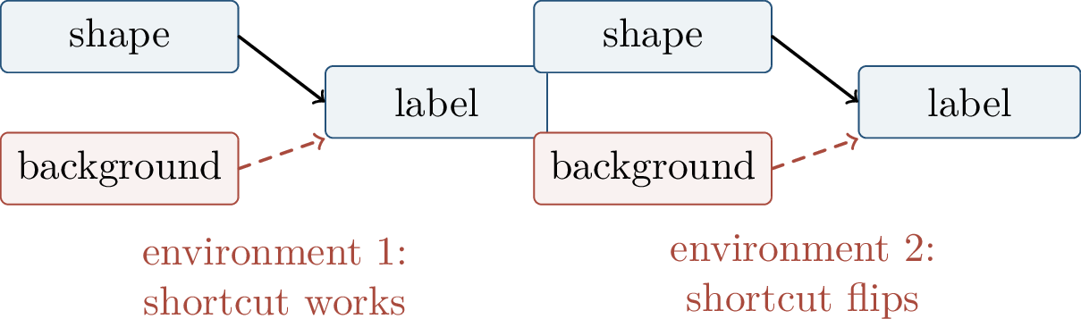
In practice, the exact IRM constraint is difficult to enforce. A common surrogate fixes a scalar classifier and penalizes environment-wise optimality gradients: \[\min_\Phi \sum_{e\in\mathcal{E}_{\mathrm{train}}}\mathcal{R}_e(\Phi) + \lambda \sum_{e\in\mathcal{E}_{\mathrm{train}}} \left\| \left.\nabla_w\mathcal{R}_e(w\circ\Phi)\right|_{w=1} \right\|^2 .\] The penalty says that a classifier trained on one environment should not need to rotate when the environment changes.
The surrogate should be read as a heuristic relaxation of the ideal constraint. It can be sensitive to scaling, parameterization, and optimization. In simple linear settings it captures the desire for a common optimal classifier; in large neural networks it is one bias among many. The scientific question is whether the chosen environments make the invariant predictor identifiable.
Definition 0.107 (Risk extrapolation). Risk extrapolation penalizes disagreement of environment risks: \[\min_f \sum_{e\in\mathcal{E}_{\mathrm{train}}}\mathcal{R}_e(f) + \lambda\, \Var_{e\in\mathcal{E}_{\mathrm{train}}}\!\big(\mathcal{R}_e(f)\big).\] Rather than only seeking a common optimal classifier, REx asks the risks to move together across environments.
REx is less tied to a specific invariant classifier constraint. By penalizing risk variance, it discourages solutions that perform well in one environment only by failing in another. Like group DRO, it depends on observed environments; like IRM, it is motivated by the hope that stable mechanisms produce balanced performance under environment changes. It is not a proof of target robustness unless the target environment is related to the observed ones.
Invariant and robust objectives rely on the environment design. They can fail when there are too few environments, when environment labels do not expose the mechanism, when the representation collapses to invariant but uninformative features, or when the nonconvex constrained optimization problem is poorly solved. Empirical benchmark studies such as DomainBed and WILDS emphasize that model selection, data coverage, and comparable tuning budgets can matter as much as the named OOD algorithm.
5.0.49 Detection, Uncertainty, and Calibration↩︎
OOD detection is not the same as OOD generalization. A predictor tries to be right on the target distribution. A detector tries to know when prediction is unsafe.
This distinction matters in deployment. A medical classifier that abstains on every image from a new scanner has excellent accepted-set accuracy but poor coverage. A language model that flags every unfamiliar legal question as OOD may avoid false confidence but fail to be useful. The deployment problem is usually a joint one: predict correctly when the model has enough support, and route or abstain when it does not.
Definition 0.108 (OOD detection and selective prediction). Given \(x\), OOD detection tests \[H_0: x\sim P_{\mathrm{ID}} \qquad H_1: x\sim Q_{\mathrm{OOD}}.\] A detector uses a score \(s(x)\) and threshold to decide whether to predict, abstain, or route to a safer system. A selective predictor aims for high coverage and low accepted-set error.
Definition 0.109 (Maximum softmax probability). For logits \(z_k(x)\), define \[p_{\max}(x)=\max_k \softmax(z(x))_k .\] Low \(p_{\max}\) is a simple baseline signal for uncertainty or OOD behavior. The method requires no retraining, but neural networks can be confidently wrong far from the training distribution.
The failure mode is calibration under shift. Softmax probabilities are normalized relative scores among known classes; they need not measure whether the input belongs to any known class at all. A model can assign high maximum softmax probability to an OOD input if one logit is accidentally much larger than the others. This is why maximum-softmax detection is a useful baseline rather than a sufficient safety mechanism.
Definition 0.110 (Energy score). For temperature \(T>0\), define \[E(x) = -T\log\sum_{k=1}^{K}\exp\big(z_k(x)/T\big).\] An energy detector chooses a threshold \(\tau\) and rejects when \(E(x)>\tau\). After suitable training or calibration, in-distribution examples often have lower energy than OOD examples.
Energy scores use the log-sum-exp of logits rather than only the largest softmax probability. They can separate ID and OOD examples better in some settings, but they still require calibration on representative validation data. The threshold \(\tau\) is part of the system design: moving it changes coverage, false rejections, and false acceptances.
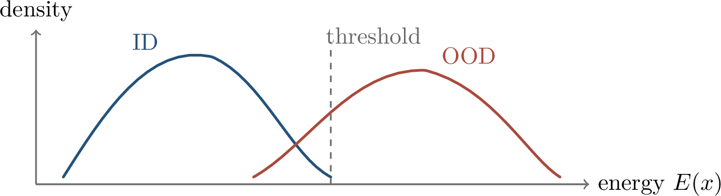
Predictive uncertainty also changes under dataset shift. A Bayesian or ensemble predictor estimates \[p(y\mid x,\mathcal{D}) = \int p(y\mid x,\theta)\,p(\theta\mid\mathcal{D})\,d\theta.\] Moving away from the training support can increase epistemic uncertainty. Empirically, deep ensembles often improve calibration under moderate shift, but severe semantic shift can still produce confident failures. This is why OOD detection, uncertainty estimation, and robust prediction must be evaluated together.
Split conformal prediction builds a set \(C_\alpha(x)\) satisfying \[\Prob\big(Y\in C_\alpha(X)\big)\ge 1-\alpha\] under exchangeability of the calibration and test examples. The guarantee is distribution-free but not distribution-shift-free: if the target distribution differs from the calibration distribution, the exchangeability condition is violated.
Under covariate shift, if \(P(Y\mid X)=Q(Y\mid X)\) and the density ratio \[w(x)=\frac{dQ_X}{dP_X}(x)\] is available, weighted conformal methods can target \(Q\)-coverage. The price is that estimating \(w(x)\) in high dimension is itself an OOD problem.
The conformal result is a good example of the theme of the chapter. The guarantee is strong once its assumptions hold, but the assumptions are about the data-generating process, not only about the algorithm. If calibration examples are exchangeable with deployment examples, coverage is distribution free. If deployment shifts, one must either collect calibration data from the target domain, model the shift, or accept that the finite-sample coverage guarantee no longer applies as stated.
A detector can succeed by abstaining on unfamiliar inputs even if the underlying predictor has not learned the target rule. Conversely, a predictor can fail under subtle semantic shift while remaining highly confident. Robust deployment needs both: knowing when to answer and answering correctly when accepted.
5.0.50 Foundation Models and Language Models↩︎
A foundation model is trained on a broad mixture of data sources and then adapted or prompted for downstream tasks. A simple statistical abstraction is \[P_{\rm pre} = \sum_{j=1}^{M}\alpha_j P_j,\] followed by deployment on a downstream distribution \(Q\). Broad pretraining helps by increasing coverage and learning reusable representations, but the task rule, prompt style, tool interface, or safety policy can still change. This is one reason foundation models are best viewed as general-purpose substrates whose opportunities and risks depend on downstream adaptation and deployment context [25].
Pretraining changes the OOD problem in two opposite ways. On the positive side, a broad mixture can make many target domains less exotic: the model may have seen similar language, concepts, code, images, or reasoning patterns. On the negative side, the training mixture is usually opaque and uncontrolled, so it is hard to state exactly which target distributions are covered. A model can look robust because a benchmark resembles pretraining data, while still failing under a shift in goals, interaction protocol, or hidden assumptions.
In-context learning can be interpreted as target adaptation at inference time. Prompt examples provide information about the local task, and the model uses its pretrained prior to convert that context into a prediction rule. This can reduce shift when the examples identify the right mechanism; it can also amplify the wrong cue when the context is misleading or too narrow.
This makes prompts analogous to a tiny target dataset. A few examples can specify a label convention, output format, domain vocabulary, or local rule. However, the prompt is not a guarantee of correct adaptation. If the examples are unrepresentative, contaminated, adversarial, or ambiguous, the model may infer a shortcut. In-context learning is therefore an OOD tool and an OOD risk at the same time.
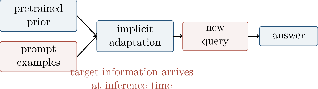
For language models, OOD shift is not only a change in input distribution. It can involve new dialects, APIs, laws, tools, adversarial prompt styles, long-context extrapolation, synthetic-to-real task mismatch, reward-model extrapolation, judge distribution shift, and changes in instruction-following behavior. The target distribution includes interaction protocols and goals, not just static examples.
Definition 0.111 (Evaluation distribution for LLMs). An LLM benchmark defines a distribution over prompts, formats, scoring rules, and judges. A schematic factorization is \[Q_{\rm eval} = Q_{\rm prompt}\times Q_{\rm format}\times Q_{\rm score}.\] Deployment can differ from any of these factors. Benchmark contamination, narrow prompt templates, and automated-judge shift are therefore distributional problems, not merely measurement annoyances.
For LLMs, the scoring rule is part of the distribution. A benchmark graded by exact match, a benchmark graded by a human rater, and a benchmark graded by an LLM judge can induce different optimization pressures. A model that adapts to one judge may not be robust to another. This is the same Goodhart logic from preference optimization, now applied to evaluation: if the score is the target, models and developers may specialize to the scoring distribution.
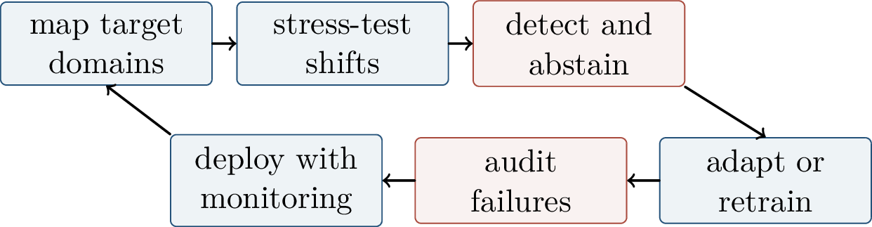
Recent theory and empirical work asks several related questions. Can a learner test whether a target distribution is safe before trusting a hypothesis? Which representations preserve invariant mechanisms rather than surface cues? When do pretrained features help or hurt OOD selection? How do reasoning traces, context length, and test-time compute change extrapolation? The answers are not yet settled, especially for interactive LLM deployments where the data distribution depends on the model’s own behavior.
This feedback loop is a new feature of foundation-model deployment. A model’s outputs influence users, users adapt their prompts, automated evaluators shape future training data, and fine-tuning changes the policy that will be deployed next. The target distribution is not fixed once and for all. OOD robustness for foundation models is therefore closer to monitoring a dynamical system than to certifying a static classifier.
5.0.51 Frontier Lessons and Open Problems↩︎
Several lessons are now stable. Target risk needs a source-risk term, a distribution-gap term, and a shared-solution term. Support mismatch makes source-only guarantees impossible without additional assumptions. Group DRO protects observed groups, while invariance methods try to identify stable mechanisms. Detection and calibration reduce harm but do not replace target competence.
At the same time, many open problems remain. Environments may be chosen by the data collector, discovered automatically, or only observed implicitly. Benchmarks can be misspecified if they mostly move along an accuracy axis rather than stressing the unstable mechanism of interest. Foundation models may appear robust because pretraining covers many cases, but may still fail under causal, semantic, or protocol shifts. Alignment and fine-tuning change the policy and therefore change the deployment distribution. Test-time compute can improve empirical extrapolation, but certifiable OOD robustness is still a much stronger target.
OOD generalization is not one problem; the shift model defines the theorem. Invariance and DRO are useful only when the environments expose the right variation. OOD detection reduces harm, but it does not replace target-domain competence. Foundation models move the frontier from static datasets toward tasks, prompts, tools, goals, and continual monitoring.
Chapter Synthesis
OOD generalization is a deployment problem: low source risk implies low target risk only under assumptions relating the source and target environments.
Domain adaptation bounds decompose target error into source error, distribution discrepancy, and shared-solution error; the last term captures whether the same classifier can work on both domains.
Support mismatch creates impossibility for source-only learners unless target labels or stable mechanisms are constrained.
Group DRO protects observed groups, while IRM and REx try to exploit environment variation to identify stable predictors.
OOD detection, uncertainty, and conformal prediction help decide when to abstain or route, but detection is not the same as robust prediction.
Foundation models reduce some shifts through broad pretraining and in-context adaptation, yet they introduce new shifts in prompts, tools, judges, interaction protocols, and feedback loops.
Core sources include Ben-David et al., A Theory of Learning from Different Domains [63]; Ganin et al., Domain-Adversarial Training of Neural Networks; Hendrycks and Gimpel, A Baseline for Detecting Misclassified and Out-of-Distribution Examples; Sagawa et al., Distributionally Robust Neural Networks for Group Shifts; Arjovsky et al., Invariant Risk Minimization; Ovadia et al., Can You Trust Your Model’s Uncertainty Under Dataset Shift; Liu et al., Energy-Based Out-of-Distribution Detection; Krueger et al., Out-of-Distribution Generalization via Risk Extrapolation; Gulrajani and Lopez-Paz, In Search of Lost Domain Generalization; Koh et al., WILDS; and Angelopoulos and Bates, A Gentle Introduction to Conformal Prediction. For the foundation-model perspective, see Bommasani et al., On the Opportunities and Risks of Foundation Models [25]. Recent directions include Harun et al., What Variables Affect OOD Generalization in Pretrained Models?; Chandrasekaran et al., Learning Neural Networks with Distribution Shift; Tang et al., Benign Overfitting in OOD Generalization of Linear Models; Salaudeen et al., Are Domain Generalization Benchmarks with Accuracy on the Line Misspecified?; Potapczynski et al., Understanding and Relaxing the Limitations of Transformers for Linear Algebra; Wang et al., Learning Minimal Contexts: How CoT Induces OOD Generalization; and Casademunt et al., Steering OOD Generalization with Concept Ablation Fine-Tuning.
5.0.52 Emergence as an Observable and a Limit↩︎
In informal discussion, an ability is called emergent when a model appears unable to perform a task below some scale and then suddenly succeeds above that scale. This description is useful but incomplete. It does not specify what is being scaled, what distribution of questions is being used, how success is measured, or whether the apparent jump is caused by the metric, by finite-size effects, or by the formation of a new internal mechanism. The empirical literature on large language models made this question prominent, while subsequent critiques showed that some apparent jumps can be induced by metric choice rather than a discontinuous latent capability [59], [60].
The mathematical way to begin is to name both the sequence and the observable. Only then can one ask whether a sharp transition is real, a limiting artifact, or a measurement artifact.
Definition 0.112 (Ability observable). Let \(M_s\) be a sequence of models indexed by scale, training time, data diversity, context length, post-training pressure, or another parameter \(s\). For a task condition \(\lambda\), define an ability observable \[A_s(\lambda) = \E_{(x,y)\sim\mathcal{D}_\lambda} \big[m(M_s,x,y)\big]\in[0,1],\] where \(m\) is a chosen scoring function. The model sequence, the distribution \(\mathcal{D}_\lambda\), and the metric \(m\) are all part of the definition.
Definition 0.113 (Emergence candidate). An observable \(A_s(\lambda)\) is an emergence candidate if there is a critical region \(\lambda_c\) such that each finite curve is smooth, but \[A_s(\lambda)\to A_\infty(\lambda), \qquad A_\inftychanges sharply near\lambda_c.\] This does not yet prove a new mechanism. It says that the limiting observable has a sharp feature that finite systems approach.
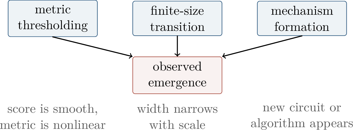
This chapter takes a deliberately decompositional view. We do not treat “emergence” as an explanation. We treat it as a hypothesis to be broken into observables, diagnostics, solvable models, training dynamics, and mechanisms. The research problem is to turn a sudden ability into a theorem, a phase diagram, and an intervention.
Definition 0.114 (Limit-speed lens). For a large-model family, write the generalization or ability gap as a random functional \[\epsilon_{\mathrm{gen}}(N,P,\partial\ell),\] where \(N\) is training-data scale, \(P\) is model size or architectural scale, and \(\partial\ell\) is a training-loss optimality gap. The limiting object is \[\epsilon_{\mathrm{gen}}(\infty,\infty,0).\] Emergence is then studied through both the limit value and the speed at which finite models approach it.
The limit-speed lens separates two questions. First, does the idealized limit have the ability? Second, are the finite errors small enough that a real model crosses the task margin? A finite model becomes credible on a query family only when its approximation to the limiting mechanism beats the required margin.
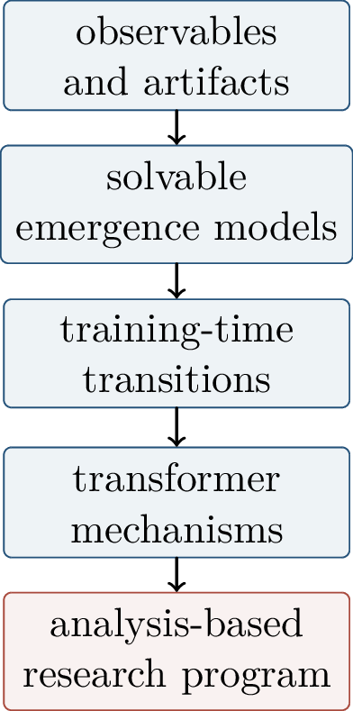
5.0.53 Metrics, Slices, and Apparent Jumps↩︎
The first diagnostic for any emergence claim is the metric. Many benchmarks convert a continuous latent score into a binary success indicator. This can turn smooth progress into an apparent cliff.
Definition 0.115 (Binary ability from a latent score). Let \(Z_s\) be a continuous score for a model at scale \(s\), and let \(\tau\) be a task-specific threshold. A binary benchmark reports \[A_s=\Prob\{Z_s>\tau\}.\] Even if the distribution of \(Z_s\) changes smoothly with \(s\), the thresholded observable can change sharply.
Example 0.22 (Metric-induced emergence). Suppose a latent score changes gradually with scale, for instance \[z_s=a\log s+b.\] The thresholded metric \[A_s=\mathbf{1}\{z_s>\tau\}\] can jump from \(0\) to \(1\) at the threshold even though the latent score has no discontinuity. This is the mechanism behind many metric-artifact explanations of reported emergent abilities.
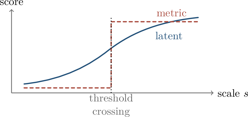
The diagnostic lesson is simple: before claiming emergence, replace exact-match accuracy by a continuous score when possible, condition on task difficulty, vary the prompt distribution, remove in-context demonstrations, and search for internal progress measures that move before the visible jump. An emergence claim is stronger when it survives metric, slice, prompt, and mechanism checks.
Slice diagnostics are especially important. A benchmark may combine easy and hard subsets: \[A_s=\pi A_s^{\rm easy}+(1-\pi)A_s^{\rm hard}.\] If easy examples degrade or saturate while hard examples improve, the aggregate can look stagnant and then suddenly rise, even though each slice is more interpretable.
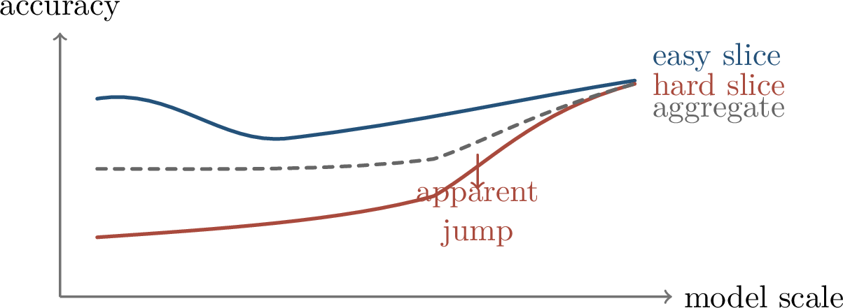
In-context learning is another confounder. Some abilities attributed to large-model emergence can be decomposed into memory, linguistic knowledge, and task inference from examples in the prompt. A claim about the pretrained model should therefore compare zero-shot, few-shot, and instruction-only settings and treat the prompting protocol as part of the observable.
Definition 0.116 (Mechanistic emergence). A capability is mechanistically emergent if there exists a latent mechanism \(H_s\) such that \[H_s\to H_\infty,\qquad A_s=\Phi(H_s)+o(1),\] and \(H_\infty\) is qualitatively different from the small-scale mechanism. Examples include induction heads, modular-arithmetic circuits, or planning-token hierarchies. Evidence should include interventions such as ablation, activation patching, synthetic controls, or causal tracing; the grokking and mechanistic-interpretability literature provides a useful model for this style of evidence [23], [58].
5.0.54 Solvable Models of Emergence↩︎
Empirical curves alone rarely explain why a threshold appears. Toy models are valuable when they produce computable thresholds, transition widths, and mechanisms. A useful toy model should be smaller than a full LLM but still contain a real bottleneck. It should predict a curve, not merely offer an analogy.
5.0.54.1 Skill Quantization and Sparse Parity
Definition 0.117 (Skill quantization model). Assume a model learns discrete skill quanta \(q_i\) with usage frequencies \(p_i\). A simple aggregate loss model is \[loss(s) \approx \sum_{i:\;q_i\;{\rm not\;learned\;at}\;s} p_i.\] If the \(p_i\) follow a heavy-tailed law and quanta are learned from high to low frequency, aggregate loss can be smooth while individual rare abilities appear suddenly.
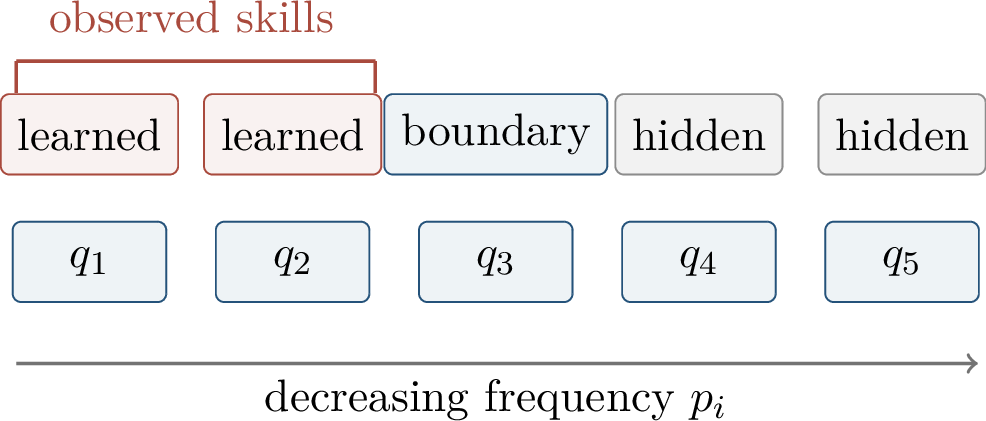
The multitask sparse parity model makes this idea more concrete. Tasks are basis functions \(\phi_j\), and the target is sampled from a heavy-tailed task distribution: \[f(x)=\sum_{j=1}^{K} a_j\phi_j(x), \qquad \Prob(j)\propto j^{-\alpha}.\] Learning each basis direction has a sigmoidal curve. A power-law task distribution creates smooth aggregate loss and abrupt individual skill acquisition. The threshold depends on data, model size, and training time, and neural-network simulations can be compared with a solvable multilinear skill model.
5.0.54.2 Percolation and Linear-Attention ICL
Another route is data-centric. Suppose the model must learn enough underlying regularities of a grammar to connect a task-relevant component. Then \[capability appears \quad\Longleftrightarrow\quad a learned-regularity graph percolates.\] Nodes are local grammar regularities or concepts; edges are compositional compatibilities; the threshold is the appearance of a giant usable component.
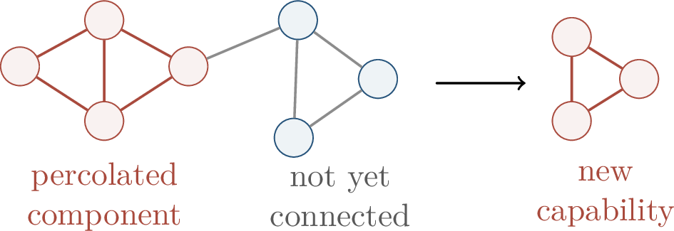
For in-context learning, high-dimensional linear attention gives a cleaner limit theory. In linear-regression prompts, take a joint limit \[d,n,\ell,k\to\infty,\qquad \frac{\ell}{d}\to\alpha,\quad \frac{k}{d}\to\kappa,\quad \frac{n}{d^2}\to\tau.\] Low task diversity leads to memorization of pretraining tasks; high diversity leads to genuine in-context generalization to new tasks. This is a clean example of emergence as a high-dimensional limit rather than as an anecdotal benchmark jump.
Skill quantization shows how aggregate smoothness can hide discrete abilities. Sparse parity gives analytically tractable individual skill curves. Percolation models show how data regularities can create critical thresholds. Linear-attention ICL separates memorization from in-context generalization through asymptotic phase diagrams. The frontier is moving from curve fitting toward mechanism-specific limit models.
5.0.55 Training-Time Phase Transitions↩︎
Scale is not the only axis along which an ability can emerge. Let \[A(t)=test ability after t gradient steps.\] A model may first memorize or develop a partial solution, then suddenly generalize after hidden internal variables cross a threshold. Grokking is the canonical example: train loss becomes low long before test accuracy rises [23], [58].
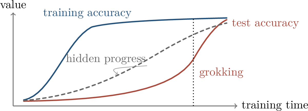
Definition 0.118 (Lazy-to-rich transition). During early training, a network may behave like kernel regression with near-fixed features. Its empirical tangent kernel is \[K_t(x,x') = \left\langle \nabla_\theta f_{\theta_t}(x),\nabla_\theta f_{\theta_t}(x') \right\rangle.\] In the lazy phase, \(K_t\approx K_0\). In the rich phase, features move and the kernel aligns better with the target.
Grokking can occur when the lazy kernel fits the training set but generalizes poorly, while later feature learning discovers a more structured representation. From this viewpoint, the visible jump is a delayed readout of a slow internal change.
Another useful abstraction is a first-order phase transition. Suppose an effective free energy \[\mathcal{F}_t(m)=U_t(m)-T S(m)\] has a memorizing minimum and a generalizing minimum. Before the transition, the memorizing state dominates. After the transition, the structured state dominates. At the critical point, the selected minimizer changes discontinuously even if the effective objective changes smoothly.
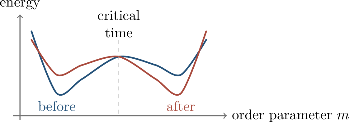
Mechanistic interpretability provides a more constructive route. Rather than asking whether a curve jumps, search for continuous progress variables \[P_1(t),\ldots,P_r(t) \quadsuch that\quad A(t)\approx \Psi(P_1(t),\ldots,P_r(t)).\] For modular addition, circuit components can be tracked in Fourier space before the visible grokking jump. In transformers, long loss plateaus can hide slow progress in attention maps or hidden-state geometry. Syntax acquisition in masked language models gives another example: a syntactic attention pattern can appear in a short training window after simpler correlations have already been learned.
To analyze an abrupt learning event, identify the visible event, track latent variables such as kernel change, attention maps, circuit coefficients, or entropy, build a reduced dynamical model for those variables, and test it by intervention. Emergence theory should predict both the visible jump time and the hidden progress curve.
5.0.56 Transformer Mechanisms↩︎
For transformers, emergence often means that a new algorithm becomes implemented in the forward pass. Few-shot behavior asks the model to infer a task from examples in the prompt. Induction behavior asks it to copy or extrapolate repeated patterns. Reasoning behavior asks it to plan, branch, verify, and revise. The mechanistic question is: which attention heads, MLP directions, or token classes implement the new algorithm? Formal studies of in-context learning show that even simple function-class or linear-regression prompts already contain nontrivial algorithmic structure [50], [51].
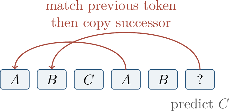
For Markov-chain data, transformers can learn to estimate transition probabilities from context: \[\widehat p(x_{t+1}=j\mid x_t=i) \approx \frac{\#(i\to j in context)}{\#(i in context)}.\] Observed phases can include uniform prediction, a unigram shortcut, and then a bigram in-context solution. A simpler intermediate solution can delay the final emergent circuit.
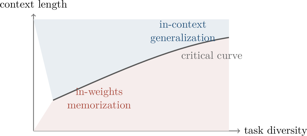
Several interpretations of in-context learning coexist. In one view, attention implements gradient descent in the forward pass. In another, the prompt defines a posterior over tasks. In a third, the model retrieves or reuses stored examples. In practice, these mechanisms can compete, and the same benchmark ability can be produced by different mechanisms under different data distributions.
Recent ICL theory separates two sub-circuits: \[in-weights learning rater_{\rm IWL}, \qquad in-context learning rater_{\rm ICL}.\] The model generalizes in context when the ICL circuit becomes useful before the memorization circuit absorbs the training tasks. The threshold depends on task diversity, context statistics, and initial conditions.
Post-training creates another emergence axis. Reinforcement learning for reasoning can separate low-level execution from high-level planning: \[procedural reliability \quad\longrightarrow\quad strategic exploration \quad\longrightarrow\quad better reasoning.\] Execution tokens may become confident before planning tokens diversify. A credit-assignment rule can then focus updates on the strategic bottleneck, creating a new phase of reasoning behavior.
Evidence for mechanistic emergence should include at least one low-dimensional feature or circuit that predicts the ability, an ablation that removes the ability, a patching intervention that restores it, and a reduced mathematical model that predicts the threshold. The goal is not a better story about emergence; it is a controllable mechanism.
5.0.57 Analysis Tools and a Limit-Speed Program↩︎
Emergence is a natural meeting point for mathematical analysis, probability, statistical physics, and mechanistic interpretability. Different tools target different parts of the phenomenon:
| Tool | What it can study |
|---|---|
| Non-uniform convergence | sharp limits from smooth finite curves |
| Finite-size scaling | critical width and threshold prediction |
| Random graph theory | percolation of data regularities |
| Random matrix theory | ICL and representation phase transitions |
| Dynamical systems | plateaus, slow variables, and bifurcations |
| Variational limits | objective changes in large models |
5.0.57.1 Three Errors and a Margin
The limit-speed lens decomposes the gap between a finite model and the ideal limit into optimization, architecture, and sample terms: \[\begin{align} \epsilon_{\mathrm{gen}}(N,P,\partial\ell)-\epsilon_{\mathrm{gen}}(\infty,\infty,0) &= \big[\epsilon_{\mathrm{gen}}(N,P,\partial\ell)-\epsilon_{\mathrm{gen}}(N,P,0)\big]\\ &\quad+ \big[\epsilon_{\mathrm{gen}}(N,P,0)-\epsilon_{\mathrm{gen}}(N,\infty,0)\big]\\ &\quad+ \big[\epsilon_{\mathrm{gen}}(N,\infty,0)-\epsilon_{\mathrm{gen}}(\infty,\infty,0)\big]. \end{align}\] The first term is an optimization gap; the second is an architecture gap; the third is a sample gap.
Definition 0.119 (Limit architecture and margin criterion). Let \(M_{N,P,\partial\ell}\) approach an idealized limit architecture \(M_{\infty,\infty,0}\). For a query family \(q\), suppose the limiting ability margin is \[\Delta(q)=A(M_{\infty,\infty,0};q)-\tau>0.\] Finite models exhibit the ability whenever \[optimization error + architecture error + sample error <\Delta(q).\]
A schematic bound from the chapter is \[\begin{align} \left|\epsilon_{\mathrm{gen}}(N,P,\partial\ell)-\epsilon_{\mathrm{gen}}(\infty,\infty,0)\right| &\lesssim \underbrace{\beta(N,P)^{1/\left\lVert \partial\ell \right\rVert^2}}_{\rm optimization}\\ &\quad+ \underbrace{\min\!\left\{C\operatorname{Lip}(T)^P,\; C e^{-m(A)\rho(P)}\right\}}_{\rm architecture}\\ &\quad+ \underbrace{C N^{-(\alpha+\kappa)/(2\alpha+2\kappa+d)}}_{\rm sample}. \end{align}\] Here \(\alpha\) represents smoothness of the target, \(d\) the data dimension, \(\kappa\) an architecture assembly effect, and \(\rho(P)\) a scale-dependent architecture quantity. The specific constants are schematic, but the form is important: emergence is a margin-versus-error problem.
5.0.57.2 Non-Uniform Limits and Finite-Size Scaling
Definition 0.120 (Non-uniform emergence template). Construct smooth finite observables \(A_s:[0,1]\to[0,1]\) such that \[A_s(\lambda)\to A_\infty(\lambda)=\mathbf{1}\{\lambda>\lambda_c\}.\] Pointwise convergence explains the sharp limiting curve, while failure of uniform convergence identifies the critical region. The transition width \(w_s\) is the object to estimate.
Near a critical point, a finite-size scaling ansatz is \[A_s(\lambda) = F\!\left((\lambda-\lambda_c)s^{1/\nu}\right) +s^{-\omega}G\!\left((\lambda-\lambda_c)s^{1/\nu}\right) +o(s^{-\omega}).\] The threshold is \(\lambda_c\), the exponent \(\nu\) controls transition width, and \(\omega\) controls corrections to scaling. This ansatz gives a rigorous target for emergence prediction and a way to distinguish a true finite-size law from finite-data noise.
Random graphs and random matrices provide complementary routes. If \(G_s=(V_s,E_s)\) is a graph of learned regularities and \[p_s=\Prob\{(u,v)\in E_s\},\] then a capability may appear when a task-relevant component crosses a percolation threshold. In high-dimensional linear attention, core quantities can reduce to spectral transforms such as \[\frac{1}{d}XX^\top \Rightarrow \mu_{\rm MP}, \qquad m(z)=\int\frac{1}{x-z}\,d\mu_{\rm MP}(x).\] These are precise places where mathematical analysis meets transformer theory.
5.0.57.3 Dynamical Systems and Research Projects
Training-time emergence can also be modeled through slow-fast dynamics: \[\dot{u}=f(u,v),\qquad \dot{v}=\varepsilon g(u,v),\qquad 0<\varepsilon\ll1.\] Fast variables explain visible loss decrease; slow variables explain delayed capability. Plateaus become slow manifolds, abrupt learning becomes escape from a metastable region, and interventions modify the vector field.
The chapter proposes four concrete research directions. First, build synthetic tasks where \(A_s(\lambda)\) is computable and the limiting curve has a true threshold. Second, find latent progress variables \(P_s\) and show \[A_s\approx \Phi(P_s),\] separating mechanism emergence from metric emergence. Third, construct phase diagrams for ICL with variables such as task diversity, context length, frequency tail, and model depth. Fourth, model reasoning RL as a bifurcation over execution reliability and planning entropy: \[(u_t,v_t) = (execution reliability,planning entropy).\]
A minimal mathematical project is to construct a learnable sequence \(M_s\) and an observable \(A_s\) such that each finite \(A_s\) is smooth but \[A_s(\lambda)\to\mathbf{1}\{\lambda>\lambda_c\}, \qquad w_s\asymp s^{-\nu}.\] The proof should predict the threshold \(\lambda_c\), the transition width \(w_s\), and the failure of uniform convergence, and then test whether the same exponent appears in small transformers.
5.0.58 Frontiers and Takeaways↩︎
We can now state a careful position. Many reported jumps are partly explained by metric choice or task mixtures. Some jumps reflect real finite-size or training-time transitions. The most useful theory comes from solvable models with identifiable mechanisms. Transformer emergence is often competition among algorithms: memorization, retrieval, in-context learning, and planning.
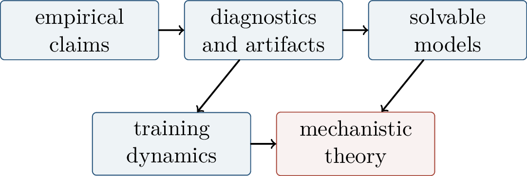
The open problems are clear. Can we prove finite-size scaling exponents for attention-based models beyond linear attention? Can progress measures be found automatically and validated causally? Can an emergence threshold be forecast from small-scale slices and internal variables? These questions ask for more than a name for sudden ability. They ask for the critical variable.
Treat emergence as a limit problem for observables. Use metrics and slices to rule out artifacts. Use solvable models to identify thresholds and exponents. Use mechanistic interventions to validate hidden variables. Turn “sudden ability” into a theorem, a phase diagram, and an experiment.
Core sources include Wei et al., Emergent Abilities of Large Language Models [59]; Schaeffer, Miranda, and Koyejo, Are Emergent Abilities of Large Language Models a Mirage? [60]; Michaud et al., The Quantization Model of Neural Scaling; Nanda et al., Progress Measures for Grokking via Mechanistic Interpretability [58]; Power et al., Grokking [23]; Kumar et al., Grokking as the Transition from Lazy to Rich Training Dynamics; Rubin, Seroussi, and Ringel, Grokking as a First Order Phase Transition in Two Layer Networks; Chen et al., Sudden Drops in the Loss; Lu et al., Are Emergent Abilities in Large Language Models just In-Context Learning?; Nam et al., An Exactly Solvable Model for Emergence and Scaling Laws in the Multitask Sparse Parity Problem; Edelman et al., The Evolution of Statistical Induction Heads; Lubana et al., A Percolation Model of Emergence; Wu and Lo, U-shaped and Inverted-U Scaling behind Emergent Abilities; Lyu, Wang, and Zhu, A Solvable Attention for Neural Scaling Laws; Lu et al., Asymptotic Theory of In-Context Learning by Linear Attention; Gopalani and Hu, What Happens During the Loss Plateau?; and Wang et al., Emergent Hierarchical Reasoning in LLMs through Reinforcement Learning. The limit-speed framework is also informed by the CASAD forum summary Large-Model Intelligent Emergence and Limit-Speed Criteria.
6 Synthesis and Research Outlook↩︎
6.1 Unified View, Limitations, and Open Problems↩︎
The preceding chapters develop many theories of deep learning. They differ in mathematical language, but they repeatedly address the same underlying issue: how a high-dimensional, overparameterized training system selects predictors that are both expressive and useful. This final chapter summarizes the common structure, compares the explanatory scope of major frameworks, and records problems that remain open.
6.1.1 A Common Template for Deep Learning Theory↩︎
Most results in the monograph can be written in a three-part form. First, one specifies an object of control: approximation error, training loss, generalization gap, stability coefficient, adversarial risk, distributional discrepancy, sampling error, or feature-level mechanism. Second, one imposes a modeling regime: smoothness, margin, width, initialization, separability, noise, distributional structure, optimization step size, or scale. Third, one deduces a guarantee or obstruction. The difference between theories lies less in this template than in the object and regime chosen.
| Framework | Controlled object | Typical limitation |
|---|---|---|
| Approximation theory | Distance from a target function to a network class | Does not specify how training finds the approximant. |
| Optimization and NTK theory | Empirical loss along gradient dynamics | Often strongest in overwide or near-kernel regimes. |
| Implicit regularization | Selected solution among many interpolants | Sensitive to parameterization, loss, and optimization path. |
| Generalization and stability | Population performance beyond the sample | May be loose or conditional in highly adaptive models. |
| Robustness and shift theory | Risk under perturbation or distribution change | Depends critically on the chosen threat or shift model. |
| Foundation-model theory | Scaling, in-context learning, internal mechanisms | Still combines empirical laws with incomplete mechanistic theory. |
This comparison is not a ranking. Each framework answers a different well-posed question. A complete theory must explain how these answers interact.
6.1.2 Where the Classical Triad Still Works↩︎
Approximation, optimization, and generalization remain the backbone of the field. Approximation theory explains why layered compositional classes can be statistically meaningful and why dimension-independent rates may be possible in structured function spaces [4], [7]. Optimization theory explains why gradient flow and gradient descent can have predictable behavior in certain overparameterized regimes [8]–[10]. Generalization theory supplies the language for sample complexity, stability, margins, and distribution-dependent control [1], [14], [15].
The limitation is that no member of the triad is sufficient alone. Expressive capacity without an optimization path is not a learning theory. Training loss without a population-risk statement is not a statistical theory. A capacity-based generalization theorem that ignores algorithmic selection may miss the decisive mechanism. The monograph therefore treats the triad as an interlocking set of constraints rather than as three independent modules.
6.1.3 Overparameterization as a Change of Regime↩︎
Overparameterization changes the meaning of classical complexity. In many modern systems the number of parameters exceeds the number of samples, yet training can interpolate and still generalize. Double descent and ridgeless regression show that the interpolation threshold is not necessarily the end of statistical performance [16], [36]. Implicit regularization shows that the algorithm may select a low-complexity solution even when the parameter space contains many interpolants [11], [12]. Kernel and NTK limits show that overwidth can linearize parts of the training dynamics, while also exposing the limitation of fixed-feature explanations.
A key open problem is to connect feature-learning regimes with generalization in a form that is both mathematically rigorous and predictive for modern architectures. Existing theories explain important boundary cases, but the transition between lazy behavior, mean-field behavior, and genuinely adaptive representation learning remains only partially understood.
6.1.4 Modern Models and New Explanatory Objects↩︎
Transformers, diffusion models, flow matching, scaling laws, sparse autoencoders, preference optimization, and foundation-model adaptation introduce objects that are not central in older supervised-learning theory. In-context learning asks whether a trained sequence model implements an algorithm over examples in its context [50], [51]. Diffusion and flow models ask how score estimation or learned transport can generate high-dimensional samples [20], [52], [53]. Scaling laws summarize the dependence of loss on model size, data, and compute [21], [54]. Mechanistic interpretability asks whether internal features and circuits can be identified and validated [22], [55], [56]. Preference optimization formalizes the relation between reward modeling, KL-regularized control, and direct policy optimization [24], [61], [62].
These topics expand deep learning theory beyond error bounds. Theoretical analysis must also account for learned algorithms, internal representations, feedback from preference data, and scale-dependent qualitative changes. This expansion motivates the subtitle of the book: the path from approximation to emergence is a path from static function classes to learned mechanisms.
6.1.5 Open Problems↩︎
Several problems recur across the chapters.
Develop generalization theories that use learned representations rather than treating the trained network as an arbitrary member of a large class.
Characterize the transition between kernel-like training and feature-learning regimes in finite-width networks.
Connect empirical scaling laws with mechanistic models that predict when additional data, parameters, or inference-time computation change capability.
Distinguish genuine emergent mechanisms from thresholding, aggregation, or metric artifacts [59], [60].
Provide robustness and distribution-shift guarantees that match the failures observed in deployed foundation models.
Build mathematically precise links between interpretability tools, causal interventions, and predictions about model behavior.
If later versions of this book include author-specific results, the cleanest placement is after this list: one can add a short paragraph explaining which open problems are addressed by the author’s published work, preprints, funded projects, or complete proofs. Such a paragraph should be factual and separately attributed, so that the present synthesis remains distinguishable from new claims.
6.1.6 Concluding Perspective↩︎
The current state of deep learning theory is plural rather than unified by a single theorem. This is not a weakness if the pluralism is made explicit. A mathematically useful account should say what each theory explains, what it assumes, and where it stops. The monograph’s contribution is to present this account in one coherent structure: classical theory supplies the baseline, overparameterization changes the regime, and modern foundation models require new explanatory objects. The resulting synthesis is intended to support further research rather than to close the subject.