Fast approximation and learning of binary classification tasks in o-minimal structures using ReLU neural networks
June 29, 2026
Abstract
We study binary classification problems whose decision sets are given by definable sets in o-minimal expansions of the real field. Motivated by cell decomposition of definable sets, we introduce traceable sets as a classical proxy for definable decision regions and analyze their approximation by ReLU neural networks. Under uniform bounds on the number of connected components and suitable \(C^m\) extensions for the boundary functions, we prove that characteristic functions of traceable subsets of \([-1/2,1/2]^n\) can be approximated in \(L^p\) to accuracy \(\varepsilon>0\) by ReLU neural networks of size \(\mathcal{O}(\varepsilon^{-p(n-1)/m})\), with depth independent of \(\varepsilon\) and polynomially bounded weights. This establishes quantitative approximation rates for certain definable collections in o-minimal structures using ReLU neural networks. The same approach also yields the stated approximation rates for a subclass of definable maps \([-1/2,1/2]^n \to \mathbb{R}\). We then combine the approximation capabilities with entropy estimates for ReLU neural network classes to obtain statistical learning rates for empirical risk minimization with hinge loss. For \(N\) uniformly distributed samples, the resulting classifiers achieve expected misclassification error of order \(N^{-m/(m+pn-p)}\) up to an arbitrarily small polynomial loss.
ReLU neural networks, binary classification, o-minimal structures, approximation rates, learning rates.
41A25, 03C64, 68T07.
1 Introduction↩︎
Deep neural networks have become one of the most successful paradigms in modern data analysis, outperforming traditional methods in a wide range of tasks, from image recognition and speech processing to natural language understanding [1]. Motivated by their empirical success, the mathematical principles governing their approximation power and statistical learnability remain an active area of research.
In particular, machine learning can be applied successfully to study binary classification problems. In a binary classification task, each data point is assigned one of two classes. Mathematically, we assume that the data vectors are contained in the box \([-1/2,1/2]^n\) for some \(n\in\mathbb{N}\) which gets partitioned into two sets \(A\) and \(A^c := [-1/2,1/2]^n\setminus A\). The classifier \(\chi_A:[-1/2,1/2]^n \to \{0,1\}\) assigns to each data vector \(v\in [-1/2,1/2]^n\) its label, \(0\) if \(v\in A\) and \(1\) if \(v\in A^c\). Classification problems are ubiquitous in applications, and their theoretical study using neural networks has led to work connecting approximation theory, statistical learning theory, and geometric regularity of decision boundaries [2]–[7].
Any quantitative result on approximation or learnability relies on a structural assumption on the target set \(A\). Some approaches rely on smoothness conditions on the boundary of \(A\), as studied in [2]. Also, boundaries given by Barron-type function classes are well-adapted to approximation and learning by ReLU neural networks [3], [6], [7]. In these cases, optimal approximation and estimation rates are known. In general, the larger the hypothesis class becomes, the weaker the achievable rates.
In this paper, we propose a different framework to study classification based on tame geometry and mathematical model theory. More precisely, we study binary classification tasks where \(A\) is definable in an o-minimal expansion of the real field and isolate properties allowing for fast approximation and learning. Definable sets in an o-minimal structure form a distinguished set system containing all semi-algebraic subsets of Euclidean space, allowing for cell decomposition theorems and a well behaved notion of dimension [8]. In particular, definable collections admit uniform finiteness properties, such as a uniform bound on the number of connected components and finite VC dimension [9], which makes them a natural candidate class for learning-theoretic analysis. Another key feature of o-minimal structures is that the composition of two definable maps is again definable. This property is not guaranteed in a Barron-type setting, leading to a workaround via the introduction of compositional function spaces [10]. But deep neural networks are built by repeatedly composing affine maps with nonlinear activation functions. Consequently, many neural network architectures fit naturally into the o-minimality framework [11].
1.1 Our contribution↩︎
Inspired by the cell decomposition theory in o-minimal structures, we isolate the analytic features needed for fast approximation with ReLU neural networks, leading to the introduction of the class of traceable sets.
Under certain technical assumptions, our first main result establishes quantitative approximation rates for characteristic functions of traceable sets using ReLU neural networks. More precisely, given a uniform bound on the number of connected components and a suitable boundary regularity condition depending on a smoothness parameter \(m\), for any \(0<\varepsilon<1/2\) and \(1\leq p < \infty\), the indicator function \(\chi_A\) of a definable set \(A \subseteq [-1/2,1/2]^n\) can be approximated in \(L^p([-1/2,1/2]^n)\) up to error \(\varepsilon\) by ReLU neural networks of size \(\mathcal{O}(\varepsilon^{-p(n-1)/m})\), with depth bounded independently of \(\varepsilon\) and weights growing at most polynomially in \(1/\varepsilon\). The main result also enables approximation of certain definable maps \(f:[-1/2,1/2]^n\to\mathbb{R}\) by ReLU neural networks. Definable functions are piecewise smooth and we show that under technical assumptions on the smoothness domains, the same rate as above can be achieved for the \(L^p\) approximation of \(f\) using ReLU neural networks, see section 7.2.
The second main result concerns recovering the decision region \(A\) for which the approximation theorem holds from randomly sampled points in \([-1/2,1/2]^n\). We derive learning rates for empirical risk minimization over the corresponding ReLU neural network approximation classes. For \(N\) independent samples drawn from the uniform distribution on \([-1/2,1/2]^n\), we obtain an upper bound of order \(N^{-m/(m+pn-p)}\) up to an arbitrarily small polynomial loss \(N^\kappa\). The proof combines the approximation theorem with entropy-based estimation arguments in the spirit of [3], thereby providing a unified approximation-and-learning theory for classification problems with suitable definable decision boundaries.
Taken together, these results suggest that definability in o-minimal structures over the real field provides a mathematically robust notion of regularity for classification theory. It captures a wide range of decision sets encountered in practice while still enabling strong approximation and estimation rates for ReLU neural networks.
1.2 Related work↩︎
We briefly outline some historical development and the interaction between machine learning and model theory that motivates the present work.
An early conceptual bridge between the two areas was established by the observation that definable collections in model-theoretic structures with the non-independence property (NIP) admit uniform combinatorial bounds. In particular, definable collections in NIP structures have finite VC dimension and are therefore PAC learnable [9]. Since o-minimal expansions of the real field satisfy NIP, this result implies PAC learnability for definable collections arising in o-minimal structures. Recently, the fundamental theorem of agnostic PAC learnability has been revisited from a model theoretic perspective studying minimal measurability requirements and giving qualitative learning guarantees for binary classification in o-minimal structures and more generally for NIP structures [12].
Following this foundational connection, further interactions between machine learning and model theory have been explored. For example, stability-theoretic ideas have been used to study online learning [13]. These developments suggest that the classical combinatorial parameters governing generalization in machine learning can often be interpreted through model-theoretic regularity properties.
Model-theoretic methods have also appeared in the study of the complexity of neural network hypothesis classes. Early work by Karpinski and Macintyre derived polynomial bounds on the VC dimension of sigmoidal neural networks and neural networks with Pfaffian activation functions [14]. This provides an explicit example where tame geometry and definability yield quantitative complexity estimates for classes of neural networks. Recently, these results have been revisited in the modern setting of machine learning for many other model classes, showing definability and PAC learnability of most practically used neural networks [11].
On the geometric side, o-minimal structures form a promising framework for tame mathematics, providing strong structural results for definable sets and functions. These include the classical cell decomposition theorems [8], but also Lipschitz cell decompositions, triangulations, and stratifications of definable sets [8], [15]–[17]. Such tools provide a rich geometric and analytic language for describing non-pathological subsets of Euclidean space, and suggest that definability can serve as a flexible regularity assumption for decision boundaries in classification problems.
More recently, o-minimality has also been proposed as a rigorous setting for studying aspects of deep learning such as optimization problems arising in training procedures of neural networks [18]. This further supports the perspective that o-minimal structures provide a natural unifying framework in which approximation theory, statistical learning, and optimization may be studied simultaneously under a common notion of tameness.
Before we state our main results, we begin by fixing notation and terminology.
2 Notation and conventions...↩︎
Throughout this paper, \(n\) ranges over \(\mathbb{N}:=\{0,1,\ldots\}\), \(m\) ranges over \(\mathbb{N}^*:= \mathbb{N}\setminus \{0\}\), and \(p\) ranges over the real interval \([1,\infty)\) and \(Q_n:=[-1/2,1/2]^n\). Further, let \([n] := \{1,\ldots,n\}\) where \([0] := \emptyset\). For a real number \(r \geq 0\), denote its integer part by \(\lfloor r \rfloor\).
2.1 ... concerning sets and maps↩︎
Suppose \(A, B\), and \(C\) are sets with \(C \subseteq A\). Denote the graph of a map \(f:A \to B\) by \(\Gamma(f) \subseteq A \times B\) and the restriction of \(f\) to \(C\) by \(f|_C\). The map with the empty graph is the empty map \(A \to B\). Further, let \(\chi_A\) be the characteristic function of \(A\) given by \(\chi_A(x):=1\) if \(x \in A\), and \(\chi_A(x):=0\) if \(x \notin A\). The power set of \(A\) is denoted as \(\mathcal{P}(A)\).
We consider \(\mathbb{R}^n\) as the usual Euclidean vector space with standard basis \(\{e_i\}_{i \in [n]}\) and use the convention that \(\mathbb{R}^0 := \{*\}\) is a singleton set. Any map \(f:\{*\}\to A\) is identified with its value \(f(\{*\}) \in A\). Further, the open and closed balls of radius \(\varepsilon>0\) around \(x \in \mathbb{R}^n\) are denoted by \(B_\varepsilon(x)\) and \(\overline{B}_\varepsilon(x)\). For \(A \subseteq \mathbb{R}^n\), we distinguish between the boundary \(\partial A := \mathop{\mathrm{cl}}(A) \setminus \mathop{\mathrm{int}}(A)\) of \(A\) and the frontier \(\mathop{\mathrm{fr}}(A) := \mathop{\mathrm{cl}}(A) \setminus A\) of \(A\).
We let \(\mathbb{R}_\infty := \mathbb{R}\cup \{\pm \infty\}\) be the ordered set extending \(\mathbb{R}\) by \(-\infty < \mathbb{R}< \infty\) and view \(\mathbb{R}_\infty\) as a topological space equipped with the order topology.
2.2 ... concerning projections and fibers↩︎
Let \(i\in[n]\). Denote the projection of \(\mathbb{R}^n\) onto the first \(i\) coordinates by \(\pi^{\leq i}_n: \mathbb{R}^n \to \mathbb{R}^i\), \((x_1,\ldots,x_n) \mapsto (x_1,\ldots,x_i)\) and \(\pi_n^{\leq 0}:\mathbb{R}^n \to \mathbb{R}^0\). We also use \(\pi_n^{< i} := \pi_n^{\leq i-1}\) and \(\pi_{n+1} := \pi_{n+1}^{\leq n}\). For the fiber of a set \(A \subseteq \mathbb{R}^n\) above \(x=(x_1,\ldots,x_i) \in \mathbb{R}^i\), we write \(A(x) := \{y \in \mathbb{R}^{n-i}: (x,y) \in A\} \subseteq \mathbb{R}^{n-i}\). So the fiber of \(A\) above \(x\) is non-empty if and only if \(x \in \pi_n^{\leq i}(A)\). Similarly, for a map \(f:A \to \mathbb{R}\), we denote the map \(A(x) \to \mathbb{R}\), \(y \mapsto f(x,y)\) by \(f(x)\), so that \(f(x)(y)=f(x,y)\). This notation causes no confusion since \(x \notin \mathop{\mathrm{dom}}(f)\) and is consistent with the usual meaning of \(f(x)\) if \(i=n\), using the convention about maps \(\mathbb{R}^0 \to \mathbb{R}\). Also, set \(A():=A\) and \(f():=f\) for the empty tuple.
2.3 ... concerning smoothness and measurability↩︎
For a \(C^m\) function \(f:U \to \mathbb{R}\), \(U \subseteq \mathbb{R}^n\) open, \(\alpha \in \mathbb{N}^n\), \(\abs{\alpha} := \alpha_1 + \cdots + \alpha_n \leq m\), let \(\partial^\alpha f: U \to \mathbb{R}\) be the continuous \(\alpha\)-th derivative of \(f\). In case \(\alpha = e_i\), we also use \(\partial^i f\) instead of \(\partial^{e_i} f\). More generally, a function \(g:A \to \mathbb{R}\) for arbitrary \(A \subseteq \mathbb{R}^n\) is \(C^m\) if there is some open \(U \subseteq \mathbb{R}^n\) with \(A \subseteq U\) and a \(C^m\) map \(f:U \to \mathbb{R}\) with \(g=f|_A\). Any function \(f:\mathbb{R}^0 \to \mathbb{R}\) is \(C^m\) using \(\partial^\alpha f = f\) for \(\alpha=()\). The empty map is \(C^m\).
As usual, the \(L^p\) norm of an \(L^p\) function \(f:\Omega \to \mathbb{R}\), \(\Omega \subseteq \mathbb{R}^n\) measurable, is \[\norm{f}_{L^p(\Omega)} := \left(\int_\Omega \abs{f}^p d\lambda^n\right)^\frac{1}{p}\] where \(\lambda^n\) is the Lebesgue measure on \(\mathbb{R}^n\). The \(L^\infty\) norm of \(f\) is given by \(\norm{f}_{L^\infty} := \mathop{\mathrm{ess sup}}_{x\in \Omega} \abs{f(x)} \in \mathbb{R}_\infty\). If \(f\) is \(C^m\) on \(\Omega\) and \(F:U\to\mathbb{R}\) is a \(C^m\) extension of \(f\) where \(\Omega \subseteq U \subseteq \mathbb{R}^n\) open, then the Sobolev norm of \(F\) is \(\norm{F}_{W^{m,\infty}(U)} :=\max_{\abs{\alpha} \leq m} \norm{\partial^\alpha F}_{L^\infty(U)}\). We set \(\norm{F}_{W^{m,\infty}(\Omega)} :=\max_{\abs{\alpha} \leq m} \norm{\partial^\alpha F}_{L^\infty(\Omega)}\) and \(\norm{f}_{W^{m,\infty}(\Omega)} := \inf_F \norm{F}_{W^{m,\infty}(\Omega)}\) where the infimum runs over all \(C^m\) extensions \(F\) of \(f\) to some open neighborhood of \(\Omega\). The empty map has norm zero.
2.4 ... concerning generalized intervals↩︎
For functions \(f,g: A \to \mathbb{R}\), \(A \subseteq \mathbb{R}^n\), such that \(f(x)<g(x)\) for all \(x\in A\), abbreviated as \(f<g\), define \[\begin{align} (f,g)_A := & \{(x,y)\in\mathbb{R}^{n+1}:x \in A, f(x) < y < g(x)\} \subseteq \mathbb{R}^{n+1}, \\ (-\infty,g)_A := & \{(x,y)\in\mathbb{R}^{n+1}:x \in A, y < g(x) \} \subseteq \mathbb{R}^{n+1}, \\ (f,\infty)_A := &\{(x,y)\in\mathbb{R}^{n+1}:x \in A, f(x) < y \} \subseteq \mathbb{R}^{n+1}, \\ (-\infty,\infty)_A:= &A \times \mathbb{R}\subseteq \mathbb{R}^{n+1}, \\ (f,f)_A := & \Gamma(f) \subseteq \mathbb{R}^{n+1}, \\ (g,f)_A := & (\infty, f)_A := (g,-\infty)_A := (\infty,-\infty)_A := \emptyset. \end{align}\] Here, the symbols \(\pm \infty \in \mathbb{R}_\infty\) are also interpreted as constant functions \(\pm \infty:A\to\mathbb{R}_\infty\).
2.5 ... concerning neural networks↩︎
For notions regarding feedforward neural networks we follow [19]. A ReLU neural network \(\Phi\) is a tuple \(((W^{(0)},b^{(0)}),\ldots,(W^{(L)},b^{(L)}))\) of matrix-vector pairs where \(L\in\mathbb{N}^*\), \(W^{(i)} \in \mathbb{R}^{d_{i+1} \times d_i}, b^{(i)} \in \mathbb{R}^{d_{i+1}}\) for \(0\leq i\leq L\) and \(d_0,\ldots,d_{L+1} \in \mathbb{N}^*\). We identify \(\Phi\) with its associated realization \[\Phi:\mathbb{R}^n \to \mathbb{R}, x \mapsto \Phi(x),\] where the output is recursively calculated by
\(x^{(0)}:=x\),
\(x^{(i)}:=\rho(W^{(i-1)}x^{(i-1)}+b^{(i-1)})\) for \(i=1,\ldots,L\),
\(\Phi(x):=W^{(L)}x^{(L)}+b^{(L)}\).
Here, \[\rho: \mathbb{R}\to \mathbb{R}, x \mapsto \max \lbrace 0,x \rbrace\] denotes the ReLU activation function. Note that we use the same letter for the realization of \(\Phi\) and typically identify the matrix-vector tuple \(((W^{(0)},b^{(0)}),\ldots,(W^{(L)},b^{(L)}))\) as an element \(\theta \in \mathbb{R}^{\sum_{i=0}^L d_{i+1}(d_i+1)}\), called the weights of \(\Phi\). Let \(\mathop{\mathrm{size}}(\Phi):= |\theta^{\neq 0}|\) be the number of non-zero weights of \(\Phi\), \(\mathop{\mathrm{width}}(\Phi):=\max_{i\in[L]} d_i\) the maximal number of neurons occurring in some layer of \(\Phi\) and \(\mathop{\mathrm{depth}}(\Phi):=L\) the number of layers of \(\Phi\). Further let \(\norm{\Phi}_{\max}:=\norm{\theta}_{\max}\) denote the maximal absolute value of the weights of \(\Phi\).
For not necessarily integer valued \(L,W,B > 0\), the class of ReLU neural networks \(\Phi: \mathbb{R}^n \to [0,1]\) where
\(\norm{\Phi}_{\max} \leq B\),
\(\mathop{\mathrm{size}}(\Phi) \leq W\),
\(\mathop{\mathrm{depth}}(\Phi) \leq L\),
is denoted by \(\mathcal{NN}(n,L,W,B)\). Note that the weights of \(\Phi \in \mathcal{NN}(n,L,W,B)\) satisfy \(\theta \in [-B,B]^j\) for some \(j \leq {2\lceil W \rceil(\lceil L \rceil \lceil W\rceil+n)}\).
3 Main results↩︎
We first state the definition of the decision sets considered in the main approximation and estimation theorems. The purpose of the so called traceable sets is isolating the properties of definable sets in o-minimal structures that enable fast approximation of their characteristic functions in \(L^p\) by ReLU neural networks.
Definition 1. Call a set \(A \subseteq \mathbb{R}^n\) \(m\)-traceable if there exist sets \(A_0,\ldots,A_n\) and bounded \(C^m\) maps \(f_i,g_i:A_{i-1} \to \mathbb{R}\) such that for each \(i\in[n]\):
\(A_i \subseteq \mathbb{R}^i\), \(A_n=A\) and \(A_0 = \{*\}\),
\(f_i<g_i\) or \(f_i=g_i\),
\(\pi_i(A_i) = A_{i-1}\) and \(A_i = (f_i,g_i)_{A_{i-1}}\).
The sequence \[(\{f_1,g_1\}, \ldots, \{f_n,g_n\})\] is called the signature datum of \(A\) and \(A_0,\ldots,A_n\) is the fundament of \(A\).
Let \(A \subseteq Q_n\) be \(m\)-traceable. If for each \(i\in[n]\), there are \(C^m\) functions \(F_i, G_i:\mathbb{R}^{i-1} \to \mathbb{R}\) with \(F_i|_{A_{i-1}} = f_i\) and \(G_i|_{A_{i-1}} =g_i\) so that \(\norm{F_i}_{W^{m,\infty}(Q_{i-1})} \leq B\) and \(\norm{G_i}_{W^{m,\infty}(Q_{i-1})} \leq B\), we say that \(A\) has the \((m,B)\)-extension property. For \(B>0\), let \(\mathcal{K}_{m,n}^B\) be the set of all \(m\)-traceable subsets of \(Q_n\) with the \((m,B)\)-extension property.
Next, we consider finite disjoint unions of \(m\)-traceable sets.
Definition 2. Let \(\ell \in \mathbb{N}\). Call a set \(\Omega \subseteq \mathbb{R}^n\) \((m,\ell)\)-traceable if there are pairwise disjoint \(m\)-traceable sets \(A^1,\ldots,A^l \subseteq \mathbb{R}^n\) for some \(l\leq \ell\) such that \(\Omega = A^1\cup\cdots\cup A^l\).
Let \(\Omega \subseteq Q_n\) be \((m,\ell)\)-traceable. Then \(\Omega\) is said to have the \((m,B,\ell)\)-extension property if there are pairwise disjoint \(A^1,\ldots,A^l \in \mathcal{K}_{m,n}^B\) for some \(l\leq \ell\) such that \(\Omega = A^1\cup\cdots\cup A^l\). Define \(\mathcal{K}_{m,n}^{B,\ell}\) to be the set of all \((m,\ell)\)-traceable subsets of \(Q_n\) which have the \((m,B,\ell)\)-extension property.
The first result concerns approximation of sets in \(\mathcal{K}_{m,n}^{B,\ell}\) by ReLU neural networks.
Theorem 1. For \(n\geq 2\), \(B>0\) and \(\ell \in \mathbb{N}\), there exist constants \(c=c(m,n,B,\ell,p)>0\) and \(s=s(m,n,B,\ell,p)>0\) so that for every \(\Omega \in \mathcal{K}_{m,n}^{B,\ell}\) and \(0<\varepsilon<1/2\), there is a ReLU neural network \(\Phi_\varepsilon^\Omega: \mathbb{R}^n \to [0,1]\) with
\(\norm{\Phi_\varepsilon^\Omega}_{\max} \leq \varepsilon^{-s}\),
\(\mathop{\mathrm{depth}}(\Phi_\varepsilon^\Omega) \leq \lceil \log_2((\ell+1) n)\rceil+(3+\lceil \log_2(m)\rceil)(14+2m/n)\),
\(\mathop{\mathrm{size}}(\Phi_\varepsilon^\Omega) \leq c\cdot\varepsilon^{-p(n-1)/m}\),
such that \[\norm{\Phi_\varepsilon^\Omega-\chi_\Omega}_{L^p(Q_n)} < \varepsilon.\]
The same rate can be achieved for a certain class of piecewise smooth functions on smoothness domains given by traceable sets, see Subsection 7.2. By Lemma 8, natural subclasses of \(\mathcal{K}_{m,n}^{B,\ell}\) come from fibers of sets contained in \(\mathcal{K}_{m,k+n}^{B,\ell}\) for \(k \geq 1\). Applying Theorem 1 in such a setting yields the following result.
Corollary 1. For \(n \geq 2,k\geq 1, B>0, \ell \in \mathbb{N}\), there exist constants \(c=c(m,n,B,\ell,p)>0\) and \(s=s(m,n,B,\ell,p)>0\) so that for every \(\Omega \in \mathcal{K}_{m,k+n}^{B,\ell}\) and \(0<\varepsilon<1/2\) and every \(a \in \mathbb{R}^k\), there is a ReLU neural network \(\Phi_\varepsilon^a:\mathbb{R}^n \to [0,1]\) with
\(\norm{\Phi_\varepsilon^a}_{\max} \leq \varepsilon^{-s}\),
\(\mathop{\mathrm{depth}}(\Phi_\varepsilon^a) \leq \lceil \log_2((\ell+1) n)\rceil+(3+\lceil \log_2(m)\rceil)(14+2m/n)\),
\(\mathop{\mathrm{size}}(\Phi_\varepsilon^a) \leq c\cdot\varepsilon^{-p(n-1)/m}\),
such that \[\norm{\Phi_\varepsilon^a-\chi_{\Omega(a)}}_{L^p(Q_n)} < \varepsilon.\]
With the approximation capabilities established, we get learning rates for the class \(\mathcal{K}_{m,n}^{B,\ell}\) via empirical risk minimization over the \(L^p\) approximating ReLU neural networks.
Theorem 2. Let \(B>0,\ell \in \mathbb{N}\), \(n \geq 2\), and \(\Omega \in \mathcal{K}_{m,n}^{B,\ell}\). For \(N \in \mathbb{N}^*\), let \(X_1,\ldots,X_N\) be independently sampled from the uniform distribution \(\lambda^n\) on \(Q_n\) and \(S:= (X_i,\chi_\Omega(X_i))_{i=1}^N\). Then an empirical risk minimizer \(\Phi_S\) with respect to the hinge loss over \[\mathcal{NN}(n,L,cN^{p(n-1)/(m+pn-p)},N^{sm/(m+pn-p)})\] with \(L:=\lceil \log_2((\ell+1)n)\rceil+(3+\lceil \log_2(m)\rceil)(14+2m/n)\) satisfies for every \(0<\kappa<p(n-1)/(m+pn-p)\), that \[\mathbb{E}_S \mathbb{E}_{X\sim\lambda^n}\abs{\chi_\Omega(X) - \chi_{[1/2,\infty)} \circ \Phi_S (X)}^2 \lesssim N^{\kappa-m/(m+pn-p)}\] where the implicit constant is independent of \(N\). Hence the minimax error can be bounded by \[\sup_{\Omega \in \mathcal{K}_{m,n}^{B,\ell}} \mathbb{E}_{(X_1,\ldots,X_N)\sim (\lambda^n)^N}\norm{\chi_\Omega -\chi_{[1/2,\infty)}\circ\Phi_S}^2_{L^2} \lesssim N^{\kappa-m/(m+pn-p)}.\]
We now explain how the results above can be applied to definable collections in o-minimal structures.
Definition 3. An o-minimal structure on \(\mathbb{R}\) is a sequence \(\mathcal{S} := (\mathcal{S}_n)_{n \in \mathbb{N}}\) such that for all \(n\):
\(\mathbb{R}^n \in\mathcal{S}_n \subseteq \mathcal{P}(\mathbb{R}^n)\),
\(A,B \in \mathcal{S}_n \implies A \cap B, A \cup B, \mathbb{R}^n\setminus A \in \mathcal{S}_n\),
\(\mathcal{S}_1\) consists of exactly the finite unions of points and open intervals in \(\mathbb{R}\),
\(\{(x_1,x_2)\in\mathbb{R}^2: x_1<x_2\} \in \mathcal{S}_2\),
\(\{(x_1,x_2,x_3)\in\mathbb{R}^3: x_1+x_2=x_3\}, \{(x_1,x_2,x_3)\in\mathbb{R}^3: x_1\cdot x_2 = x_3\} \in \mathcal{S}_3\),
\(A \in \mathcal{S}_n \implies \mathbb{R}\times A, A \times \mathbb{R}\in \mathcal{S}_{n+1}\),
\(\{ (x_1,\ldots,x_n) \in \mathbb{R}^n: x_1 =x_n \} \in \mathcal{S}_n\),
\(A \in \mathcal{S}_{n+1} \implies \pi_{n+1}(A) \in \mathcal{S}_n\).
A set \(A \subseteq \mathbb{R}^n\) is definable (in \(\mathcal{S}\)) if \(A \in \mathcal{S}_n\). A map \(f:A \to \mathbb{R}\) is definable (in \(\mathcal{S}\)) if its graph \(\Gamma(f) \subseteq \mathbb{R}^{n+1}\) is definable. Call \(\mathcal{H} \subseteq \mathcal{P}(\mathbb{R}^n)\) a definable collection if there is some definable set \(A \subseteq \mathbb{R}^k \times \mathbb{R}^n\), \(k\geq 1\), such that \(\mathcal{H} = \{A(a):a\in \mathbb{R}^k \}\). Let \(\mathcal{H} \subseteq \mathcal{P}(\mathbb{R}^n)\) be a definable collection. If \(\mathcal{H} = \{A(a):a\in \mathbb{R}^k \}\) for some \(k \geq 1\) and \(A \in \bigcup_{B>0,\ell \geq0}\mathcal{K}_{m,k+n}^{B,\ell}\), we call \(H\) \(m\)-admissible.
Corollary 1 allows the approximation of \(m\)-admissible definable collections in o-minimal structures by ReLU neural networks.
Corollary 2. Let \(\mathcal{S}\) be an o-minimal structure on \(\mathbb{R}\) and let \(\mathcal{H} \subseteq \mathcal{P}(\mathbb{R}^n)\) be a definable collection for \(n\geq 2\). If \(\mathcal{H}\) is \(m\)-admissible, then there exist constants \(c=c(\mathcal{H},m,n,p)>0\), \(s=s(\mathcal{H},m,n,p)>0\) and \(t=t(\mathcal{H},m,n,p) > 0\) such that for every \(0<\varepsilon<1/2\) and every \(H \in \mathcal{H}\), there is a ReLU neural network \(\Phi_\varepsilon^H: \mathbb{R}^n \to [0,1]\) with
\(\norm{\Phi_\varepsilon^H}_{\max} \leq \varepsilon^{-s}\),
\(\mathop{\mathrm{depth}}(\Phi_\varepsilon^H) \leq t\),
\(\mathop{\mathrm{size}}(\Phi_\varepsilon^H) \leq c\cdot\varepsilon^{-p(n-1)/m}\),
\(\norm{\Phi_\varepsilon^H-\chi_H}_{L^p(Q_n)} < \varepsilon\).
The paper is organized as follows. After the preliminaries in Section 4 on extensions of maps, Section 5 discusses fundamental results about o-minimal structures including the smooth cell decomposition theorem and definable collections. The properties of definable sets are then generalized in Section 6, studying traceable sets and their boundaries. Afterwards, in Subsection 7, the approximating ReLU neural network class is constructed and the proof of Theorem 1 is given. To complete the chapter, certain piecewise smooth functions on traceable domains are approximated by ReLU neural networks. Lastly, Section 8 is devoted to the proof of Theorem 2.
4 Preliminaries↩︎
First, we give a useful lemma concerning smoothness of fibers of functions.
Lemma 1. Let \(i<n\), \(A \subseteq \mathbb{R}^n\), and \(f:A \to \mathbb{R}\) be a \(C^m\) map. Then for each \(a \in \mathbb{R}^i\), the map \(f(a):A(a) \to \mathbb{R}\) is \(C^m\). Further, \(\norm{f(a)}_{W^{m,\infty}(A(a))} \leq \norm{f}_{W^{m,\infty}(A)}\).
Proof. As \(f\) is \(C^m\), there is some open \(U \supseteq A\) and a \(C^m\) map \(F: U \to \mathbb{R}\) such that \(F|_A = f\). Let \(a \in \mathbb{R}^i\). Then \(F(a)|_{A(a)} = f(a)\) and we claim that \(U(a) \supseteq A(a)\) is open in \(\mathbb{R}^{n-i}\) and that \(F(a): U(a) \to \mathbb{R}\) witnesses that \(f(a)\) is \(C^m\). To this end, we distinguish two cases. In case \(a \in \mathbb{R}^i \setminus \pi_n^{\leq i}(U)\), \(U(a) = \emptyset\) is open and \(F(a)=f(a):\emptyset \to \mathbb{R}\) is the empty map. If \(a \in \pi_n^{\leq i}(U)\), then for each \(b=(b_{i+1},\ldots,b_n) \in \mathbb{R}^{n-i}\) such that \((a,b) \in U\), there is some \(\delta=\delta(b) > 0\) such that \[(a,b) \in \bigtimes_{j=1}^i(a_j-\delta,a_j+\delta) \times \bigtimes_{j=i+1}^n (b_j-\delta,b_j+\delta) \subseteq U.\] Hence \(b \in \bigtimes_{j=i+1}^n (b_j-\delta,b_j+\delta) \subseteq U(a)\), so \(U(a)\) is open. In all cases, \(F(a): U(a) \to \mathbb{R}\) satisfies \(\partial^{\tilde{\alpha}} (F(a)) = (\partial^\alpha F)(a)\) for \(\alpha \in \{0\}^ i\times\mathbb{N}^{n-i}\), \(\abs{\alpha} \leq m\), \(\tilde{\alpha}=(\alpha_{i+1}, \ldots, \alpha_n)\), so \(F(a)\) is \(C^m\).
For each such \(\alpha\) and every \(C^m\) map \(F\) as above, we get \[\norm{\partial^{\tilde{\alpha}} (f(a))}_{L^\infty(A(a))}= \norm{(\partial^\alpha f)(a)}_{L^\infty(A(a))} \leq \norm{\partial^\alpha f}_{L^\infty(A)}\leq \norm{f}_{W^{m,\infty}(A)},\] so the second part follows by taking the infimum over all such \(F\). ◻
We continue with a useful notion from variational analysis to extend real valued functions [20], Chapter 1.
Definition 4. Let \(f:\mathbb{R}^n \to \mathbb{R}_\infty\). Then \(f\) is lower semi-continuous (lsc) at \(x \in \mathbb{R}^n\) if \(f(x) = \liminf_{z \to x}f(z)\) and upper semi-continuous (usc) at \(x \in \mathbb{R}^n\) if \(f(x) = \limsup_{z \to x}f(z)\). Here, \[\liminf_{z \to x}f(z) := \sup_{\delta >0} \inf_{z\in B_\delta(x)}f(z), \quad \limsup_{z \to x}f(z) := \inf_{\delta >0} \sup_{z\in B_\delta(x)}f(z).\] We say that \(f\) is lsc (resp. usc) if \(f\) is lsc (resp. usc) at every \(x \in \mathbb{R}^n\).
We let \(\Gamma^\uparrow(f) := \{(x,y) \in \mathbb{R}^n \times \mathbb{R}:f(x)\leq y\}\) be the epigraph of \(f\) and \(\Gamma^\downarrow(f) := \{(x,y) \in \mathbb{R}^n \times \mathbb{R}:f(x)\geq y\}\) be the hypograph of \(f\). The domain of \(f\) is defined as \(\mathop{\mathrm{dom}}(f):=f^{-1}(\mathbb{R})\).
Remark 3. Let \(f:\mathbb{R}^n \to \mathbb{R}_\infty\). If \(\liminf_{z \to x} f(z) = \limsup_{z \to x} f(z)\) for every \(x \in \mathbb{R}^n\), then \(f\) is continuous. Also, \(f\) is lsc if and only if \(-f\) is usc as \(\liminf_{z \to x} -f(z) = -\limsup_{z \to x} f(z)\). We have \(\Gamma^\downarrow(-f) = \{(x,-y): (x,y)\in\Gamma^\uparrow(f)\}\), \(\Gamma^\uparrow(-f) = \{(x,-y):(x,y) \in \Gamma^\downarrow(f)\}\).
Proposition 4. Let \(f:\mathbb{R}^n \to \mathbb{R}_\infty\).
If \(f\) is lsc, then \(\Gamma^\uparrow(f)\) is closed,
If \(f\) is usc, then \(\Gamma^\downarrow(f)\) is closed.
Proof. (i) Follows from [20], Theorem 1.6.
(ii) Follows from (i) and Remark 3 replacing \(f\) by \(-f\). ◻
Lemma 2. Let \(A \subseteq \mathbb{R}^n\). If \(f:A \to \mathbb{R}\) is continuous, then \(\underline{f}:\mathbb{R}^n \to \mathbb{R}_\infty\), where \[\underline{f}(x) := \begin{cases*} \sup_{\delta>0}\inf_{z \in B_\delta(x)\cap A} f(z), \quad x\in\mathop{\mathrm{cl}}(A) \\ \infty, \quad x\in\mathbb{R}^n\setminus\mathop{\mathrm{cl}}(A) \end{cases*}\] is the unique lsc extension of \(f\) such that every lsc map \(g:\mathbb{R}^n \to \mathbb{R}_\infty\) with \(g|_A \leq f\) satisfies \(g \leq \underline{f}\). Also, \(\overline{f}: \mathbb{R}^n \to \mathbb{R}_\infty\), \[\overline{f}(x) := \begin{cases*} \inf_{\delta>0} \sup_{z\in B_\delta(x)\cap A} f(z), \quad x\in\mathop{\mathrm{cl}}(A) \\ - \infty, \quad x\in\mathbb{R}^n\setminus\mathop{\mathrm{cl}}(A) \end{cases*}\] is the unique usc extension of \(f\) such that every usc map \(h:\mathbb{R}^n \to \mathbb{R}_\infty\) with \(h|_A \geq f\) satisfies \(h \geq \overline{f}\). Moreover, \(\Gamma^\uparrow(\underline{f}) \subseteq \mathop{\mathrm{cl}}(A) \times \mathbb{R}\) and \(\Gamma^\downarrow(\overline{f}) \subseteq \mathop{\mathrm{cl}}(A) \times \mathbb{R}\).
Proof. For each \(x\in A\), the continuity of \(f\) yields \[\sup_{\delta>0}\inf_{z \in B_\delta(x)\cap A} f(z) = \inf_{\delta>0} \sup_{z\in B_\delta(x)\cap A} f(z) = f(x)\] and hence \(\underline{f}\) and \(\overline{f}\) extend \(f\). By definition, \(\underline{f}\) is lsc and \(\overline{f}\) is usc. Let \(g\) and \(h\) be as claimed. Then \(\underline{f} \geq g\) and \(\overline{f} \leq h\) on \(\mathbb{R}^n \setminus \mathop{\mathrm{cl}}(A)\). For every \(x \in \mathop{\mathrm{cl}}(A)\) and \(\delta>0\), \(B_\delta(x)\cap A \neq \emptyset\) and so \[g(x) = \liminf_{z \to x} g(z) \leq \sup_{\delta>0}\inf_{z \in B_\delta(x)\cap A} f(z) = \underline{f}(x)\] and \[h(x) = \limsup_{z\to x} h(z) \geq \inf_{\delta>0} \sup_{z\in B_\delta(x)\cap A} f(z) = \overline{f}(x).\] Uniqueness follows from the properties just shown. We have that \(\Gamma^\uparrow(\underline{f}) \subseteq \mathop{\mathrm{cl}}(A) \times \mathbb{R}\) and \(\Gamma^\downarrow(\overline{f}) \subseteq \mathop{\mathrm{cl}}(A) \times \mathbb{R}\), so the second part follows. ◻
Definition 5. For a continuous function \(f:A \to \mathbb{R}\) where \(A\subseteq \mathbb{R}^n\), call \(\underline{f}\) the lsc envelope of \(f\) and \(\overline{f}\) the usc envelope of \(f\) where \(\underline{f}\) and \(\overline{f}\) as in Lemma 2.
5 O-minimal structures↩︎
Many areas of mathematics are built around distinguished classes of sets, e.g. the open sets in topology, or the measurable sets in measure theory. They are chosen to ground a rich theory and represent an interesting part of mathematics, motivated by very different reasons. In Euclidean space, o-minimal structures on the real field sit among these set systems, capturing a wide range of well-behaved sets, including all semi-algebraic sets. The core property of these rather large set systems is that each member admits a decomposition into finitely many cells. These building blocks forbid the emergence of pathological behavior of functions and exclude the construction of complicated sets: no oscillations, no space filling curves, and no infinitely complex constructions via repeated application of basic set operations. In fact, not even the integers are definable in any o-minimal structure because they have infinitely many connected components. Nonetheless, rather interesting and flexible o-minimal structures exist, as described in the examples below.
Functions and sets contained in o-minimal structures not only have many regularity properties on bounded regions, but also behave controllably on unbounded domains. For the interested reader, we mention that the one-variable definable functions in an o-minimal structure give rise to a Hardy field [21], [22].
This chapter heavily relies on [8], a source for most fundamental results of o-minimality. For the convenience of the reader, we repeat the definition 3 of an o-minimal structure on the ordered field of real numbers.
Definition 6. An o-minimal structure on \(\mathbb{R}\) is a sequence \(\mathcal{S} := (\mathcal{S}_n)_{n \in \mathbb{N}}\) such that for all \(n\):
\(\mathbb{R}^n \in\mathcal{S}_n \subseteq \mathcal{P}(\mathbb{R}^n)\),
\(A,B \in \mathcal{S}_n \implies A \cap B, A \cup B, \mathbb{R}^n\setminus A \in \mathcal{S}_n\),
\(\mathcal{S}_1\) consists of exactly the finite unions of points and open intervals in \(\mathbb{R}\),
\(\{(x_1,x_2)\in\mathbb{R}^2: x_1<x_2\} \in \mathcal{S}_2\),
\(\{(x_1,x_2,x_3)\in\mathbb{R}^3: x_1+x_2=x_3\}, \{(x_1,x_2,x_3) \in\mathbb{R}^3: x_1\cdot x_2 = x_3\} \in \mathcal{S}_3\),
\(A \in \mathcal{S}_n \implies \mathbb{R}\times A, A \times \mathbb{R}\in \mathcal{S}_{n+1}\),
\(\{ (x_1,\ldots,x_n) \in \mathbb{R}^n: x_1 =x_n \} \in \mathcal{S}_n\),
\(A \in \mathcal{S}_{n+1} \implies \pi_{n+1}(A) \in \mathcal{S}_n\).
A set \(A \subseteq \mathbb{R}^n\) is definable (in \(\mathcal{S}\)) if \(A \in \mathcal{S}_n\). A map \(f:A \to \mathbb{R}\) is definable (in \(\mathcal{S}\)) if its graph \(\Gamma(f) \subseteq \mathbb{R}^{n+1}\) is definable.
Remark 5. The o-minimality refers to the constraint that the only definable subsets of \(\mathbb{R}\) are finite unions of intervals and points. The classical definition of an o-minimal structure [8] does not include axiom (v). However, the field structure enables to define an intrinsic notion of smoothness which is essential for this paper.
Example 1. If \(\sigma:\mathbb{R}^n \to \mathbb{R}^n\) is a bijective linear map, then \(\sigma\) is definable using the formula for matrix vector multiplication. So for each \(A \in \mathcal{S}_n\) it follows that \(\sigma(A) \in \mathcal{S}_n\) as the image of a definable set under a definable map is definable.
We briefly treat an alternative way of viewing o-minimal structures through the lens of model theory. Originally, sets contained in an o-minimal structure are defined by some first order formula in the underlying language of a certain model theoretic structure interpreting a total ordering. In our own words, we sketch the formalism of first order logic, but also refer to [8], Chapter 1. For other introductory notes on mathematical logic, see for example [23].
Take sets of symbols \(X=\{x_n\}_{n}\) (variables), \(\mathcal{F}\supseteq \mathbb{R}\cup \{+,\cdot\}\) (function symbols) and \(\mathcal{R} \supseteq \{=,<\}\) (relation symbols) and assign to each \(f \in \mathcal{F}, R \in \mathcal{R}\) an arity \(n_f,n_R\in \mathbb{N}\) which is thought of as the number of inputs of \(f\) and \(R\) respectively. For example, \(n_==n_<=n_+=n_\cdot=2\) and \(n_r=0\) for all \(r\in\mathbb{R}\) (strictly speaking, we distinguish between ‘names’ of real numbers as function symbols and their interpretation as a real number).
The symbols in \(\mathcal{F} \cup \mathcal{R}\) are interpreted as functions \(f:\mathbb{R}^{n_f} \to \mathbb{R}\), and relations \(R \subseteq \mathbb{R}^{n_r}\) respectively. Terms are built inductively by successively plugging in simpler terms in functions: each variable \(x\in X\) and every constant \(r \in \mathbb{R}\) is a term and if \(f \in \mathcal{F}\) and \(t_1,\ldots,t_{n_f}\) are terms, then \(f(t_1,\ldots,t_{n_f})\) is a term.
A basic formula is a statement about certain terms being in some relation. More precisely, if \(R\in \mathcal{R}\) and \(t_1,\ldots, t_{n_r}\) are terms, then \(R(t_1,\ldots,t_{n_r})\) is a basic formula. The formulas consist of basic formulas and are closed under boolean combination and quantification: for formulas \(\phi\) and \(\psi\), also \(\phi \lor \psi\), \(\phi \land \psi,\neg \phi,\forall x \phi\) and \(\exists x \phi\) are formulas for every \(x\in X\) with their usual interpretation. If a formula has free variables not under the scope of quantifiers, then one can consider the set defined by the formula. More precisely, if \(\phi(\bar{x})\) is a formula with free variables \(\bar{x} \in X^n\) for suitable \(n\), then \[A:= \{a \in \mathbb{R}^n: \phi(a) \text{ holds}\}\] is the set defined by \(\phi\). Here, \(\phi(a)\) is a sentence with no free variables which has a binary truth value. A set that is defined by a formula is called a definable set.
If the definable sets in \(\mathbb{R}\) defined by formulas in \(\mathcal{F} \cup \mathcal{R}\) are finite unions of points and intervals, then the definable sets in \(\mathcal{F} \cup \mathcal{R}\) form an o-minimal structure on \(\mathbb{R}\). The connection between the axioms from Definition 3 and the logical operations combine syntax and semantics as follows.
Unions, intersections and complements of sets correspond to boolean connectives \(\lor,\land\) and \(\neg\) applied to their defining formulas,
Projections onto certain coordinates correspond to existential quantification over corresponding variables,
Diagonals correspond to equalities among variables.
On the other hand, for a given o-minimal structure \(\mathcal{S}\), viewing every element of \(\mathcal{S}\) as the interpretation of a relation symbol in the language having for each \(A \in \mathcal{S}_n\) a distinguished relation symbol \(R_A\) with arity \(n\) interpreted as \(A \subseteq \mathbb{R}^n\) yields a model theoretic structure. This follows from the closure properties of o-minimal structures which ensure that no new definable sets arise from \(\mathcal{S}\), hence \(\mathcal{S}\) consists of exactly the definable sets of the described model theoretic structure.
We continue with some examples of well known o-minimal structures.
Example 2. The semi-algebraic sets of \(\mathbb{R}\) are described by the definable sets using the symbols \(\mathcal{F} \cup \mathcal{R} =\mathbb{R}\cup \{+,\cdot,=,<\}\), an o-minimal structure \(\mathcal{S} = (\mathcal{S}_n)_{n \in \mathbb{N}}\) where \(\mathcal{S}_n\) consists of finite unions of sets of the form \(\{x \in \mathbb{R}^n: p_1(x) > 0,\ldots, p_\ell(x) > 0,p(x)=0\}\) for polynomials \(p,p_1,\ldots,p_\ell \in \mathbb{R}[X_1,\ldots,X_n]\), \(\ell\in\mathbb{N}\) [8]. A function is semi-algebraic if its graph is semi-algebraic. Any ReLU neural network is semi-algebraic [11].
Other interesting examples include \(\mathbb{R}_{\exp}\), where \(\mathcal{F} \cup \mathcal{R}= \mathbb{R}\cup \{\exp,+,\cdot,=,<\}\), interpreting \(\exp:\mathbb{R}\to\mathbb{R}\) as the usual exponential function, and \(\mathbb{R}_{\mathop{\mathrm{an}}}\), containing for each \(n\) all restricted analytic functions \(\mathbb{R}^n \to \mathbb{R}\) given by real analytic functions in \([-1,1]^n\) extended by zero. Also the amalgamation \(\mathbb{R}_{\mathop{\mathrm{an}},\exp}\) of \(\mathbb{R}_{\exp}\) and \(\mathbb{R}_{\mathop{\mathrm{an}}}\) is an o-minimal structure [24]. A more general source of o-minimal structures are quasi-analytic Denjoy-Carleman classes whose functions are locally given by their Taylor series [25]. Although classical Weierstrass preparation fails for quasi-analytic Denjoy-Carleman classes, other resolutions of singularities apply to control the number of connected components of definable sets using a normalization algorithm as shown in [25].
Also, Pfaffian functions form an o-minimal structure [26]. A Pfaffian function \(f:\mathbb{R}^n \to \mathbb{R}\) is constructed via a sequence \(f_1,\ldots,f_k = f\), \(k\in\mathbb{N}\) of \(C^1\) functions such that \[\partial^j f_i \in \mathbb{R}[x_1,\ldots,x_n,f_1,\ldots,f_i]\] for all \(i\in[k],j\in[n]\). For example, \(\arctan\) is a Pfaffian function which is witnessed by the sequence \(f_1(x) = 1/(x^2+1), f_2(x) =\arctan(x)\) as \(f_1'(x) = -2x/(x^2+1)^2 = -2xf_1(x)^2\) and \(f_2'(x) = 1/(x^2+1)=f_1(x)\).
For many other examples of definability of practically relevant functions in o-minimal structures, see [11].
5.1 Cells in o-minimal structures↩︎
Let \(\mathcal{S} = (\mathcal{S}_n)_{n \in \mathbb{N}}\) be an o-minimal structure on \(\mathbb{R}\). First, we are interested in concrete descriptions of definable sets in higher dimensions. The axioms of o-minimal structures on \(\mathbb{R}\) give exhaustive information for definable sets contained in \(\mathbb{R}\) and the cell decomposition theorem shows that a similar flavor is reflected in higher dimensions. In fact, every definable set has finitely many connected components and is built up from sets of a special shape. We are particularly interested in bounded definable sets \(A \subseteq Q_n\), leading to the definition of bounded \(C^m\)-cells. To state the inductive definition of a \(C^m\)-cell, we refine the notion of smoothness.
Definition 7. Let \(A \subseteq \mathbb{R}^n\) be definable and \(f:A \to \mathbb{R}\) definable. Then \(f\) is said to be definably \(C^m\) if there is some definable open set \(U \supseteq A\) and a definable map \(F:U \to \mathbb{R}\) such that \(F|_A = f\) and \(F\) is \(C^m\), i.e. for each \(\alpha \in \mathbb{N}^n\), \(\abs{\alpha} \leq m\), the map \(\partial^\alpha F: U \to \mathbb{R}\) exists and is continuous.
Remark 6. Every definable map \(f:A \to \mathbb{R}\) for \(A \subseteq \mathbb{R}^n\) which is definably \(C^m\) is also \(C^m\) in the usual sense, witnessed by the same (definable) open \(U\) and (definable) map \(F\).
Definition 8. Let \((i_1,\ldots,i_n) \in \{0,1\}^n\). We define inductively when \(C \subseteq \mathbb{R}^n\) is an \((i_1,\ldots,i_n)\)-\(C^m\)-cell.
The only \(()\)-\(C^m\)-cell is \(\mathbb{R}^0:=\{*\}\),
Suppose that \(C \subseteq \mathbb{R}^n\) is a \((i_1, \ldots, i_n)\)-\(C^m\)-cell and \(f,g:C \to \mathbb{R}\) are bounded maps which are definably \(C^m\) with \(f=g\) or \(f<g\). Then \((f,g)_C \subseteq \mathbb{R}^{n+1}\) is a
\((i_1, \ldots, i_n,0)\)-\(C^m\)-cell if \(f=g\),
\((i_1, \ldots, i_n,1)\)-\(C^m\)-cell if \(f<g\).
The \(C^m\)-cells of \(\mathcal{S}\) are all \((i_1,\ldots,i_n)\)-\(C^m\)-cells for every \(n\) and \((i_1,\ldots,i_n) \in \{0,1\}^n\). The signature of a \(C^m\)-cell \(C \subseteq \mathbb{R}^n\) is the unique sequence \((i_1,\ldots,i_n) \in \{0,1\}^n\) so that \(C\) is an \((i_1,\ldots,i_n)\)-\(C^m\)-cell. Further, the dimension \(\dim(C) \in \{0,\ldots,n\}\) of \(C\) is defined as \(\dim(C) := i_1+\cdots+i_n\).
Let \(A \subseteq \mathbb{R}^n\) be a bounded definable set. We consider partitions of \(A\) into \(C^m\)-cells.
Definition 9. A \(C^m\)-cell decomposition \(\mathcal{C}\subseteq \mathcal{P}(A)\) of \(A\) is a partition of \(A\) into finitely many \(C^m\)-cells such that \(\mathcal{C}_i:=\{\pi_n^{\leq i}(C): C \in \mathcal{C}\}\) is a \(C^m\)-cell decomposition of \(\pi_n^{\leq i}(A)\) for all \(i\in[n]\). A \(C^m\)-cell decomposition of \(\pi_n^{\leq 1}(A)\) is a partition of \(\pi_n^{\leq 1}(A)\) into finitely many intervals and points. We say that \(\mathcal{C}\) is compatible with a definable set \(B \subseteq A\) if \(B\) is a union of \(C^m\)-cells in \(\mathcal{C}\).
We state a bounded version of the \(C^m\)-cell decomposition theorem, the main structural result about definable functions and sets [8], (3.3), or [27], Theorem 6.6.
Theorem 7. For definable sets \(A_1,\ldots, A_\ell \subseteq A,\ell\in\mathbb{N}\), and any definable function \(f:A \to \mathbb{R}\), there is a \(C^m\)-cell decomposition \(\mathcal{C}\) of \(A\) compatible with \(A_i\) for each \(i\in[\ell]\) and such that \(f|_C\) is \(C^m\) for every \(C^m\)-cell \(C \in \mathcal{C}\).
Remark 8. For an infinite collection \(\mathcal{B}\) of definable sets, the number of \(C^m\)-cells needed to decompose a member of \(\mathcal{B}\) might be arbitrarily large, but there are certain natural classes of definable sets, called definable collections, which admit uniform upper bounds on the number of \(C^m\)-cells needed to decompose each individual member, see Subsection 5.2.
Lemma 3. Let \(C \subseteq \mathbb{R}^n\) be a \(C^m\)-cell and \(f:C \to \mathbb{R}\) definably \(C^m\) and \(i<n\). Then for each \(a \in \pi_n^{\leq i}(C)\), the map \(f(a):C(a) \to \mathbb{R}\) is definably \(C^m\).
Proof. As \(f\) is definably \(C^m\), there is some definable open \(U \supseteq C\) and a definable function \(F: U \to \mathbb{R}\) such that \(F|_C = f\) and for all \(\alpha \in \mathbb{N}^n\), \(\abs{\alpha} \leq m\), the map \(\partial^\alpha F: U \to \mathbb{R}\) exists and is continuous. Let \(a \in \mathbb{R}^i\). Then \(U(a) \supseteq C(a)\) is definable and as in the classical case in Lemma 1, \(U(a)\) is open in \(\mathbb{R}^{n-i}\) and \(F(a): U(a) \to \mathbb{R}\) witnesses that \(f(a)\) is \(C^m\). As \(F(a)\) and \(U(a)\) are definable, this gives that \(f(a)\) is definably \(C^m\). ◻
5.2 Definable collections↩︎
Natural potentially infinite classes of definable sets are given by definable collections that consist of fibers of high dimensional definable sets. The advantage of definable collections is that the number of \(C^m\)-cells needed to decompose an individual fiber is uniformly bounded. This also reflects the fact that o-minimal structures have NIP, making definable collections PAC learnable [9]. Another instance of this result is finite sample complexity for most modern architectures of neural networks [11].
Definition 10. Let \(A \subseteq \mathbb{R}^n\) and \(D \subseteq \mathbb{R}^i,i<n\) be both definable. Call \[\mathcal{A}_{i,D} :=\{A(a) \subseteq \mathbb{R}^{n-i}:a\in D\} \subseteq \mathcal{P}(\mathbb{R}^{n-i})\] the definable collection coming from \(A\) with parameter space \(D \subseteq \mathbb{R}^i\). Then a collection \(\mathcal{H} \subseteq \mathcal{P}(\mathbb{R}^{n-i})\) is definable if there is some definable set \(A \subseteq \mathbb{R}^n\) such that \(\mathcal{H}=\mathcal{A}_{i,\mathbb{R}^i}\).
Remark 9. Suppose \(\mathcal{A}_{i,D}\) is the definable collection coming from \(A\) with parameter space \(D \subseteq \mathbb{R}^i, i<n\). For a definable injective map \(h:\mathbb{R}^i \to Q_i\), there is some definable \(A'\subseteq \mathbb{R}^n\) with \(\mathcal{A}'_{i,h(D)} = \mathcal{A}_{i,D}\). Hence the parameter space of a definable collection can be augmented to \(Q_i\) by setting a default value on \(Q_i \setminus h(D)\). Such a map always exists as scaling down coordinates via the map \(x \mapsto x/\sqrt{4+4x^2}\) is definable.
Let \(A \subseteq \mathbb{R}^n\) be definable. The next statement illustrates that \(C^m\)-cell decompositions of high dimensional definable sets yield \(C^m\)-cell decompositions of fibers thereof, and thus give a uniform bound on the number of \(C^m\)-cells needed to decompose each fiber [8].
Lemma 4. Every \(C^m\)-cell decomposition \(\mathcal{C}\) of \(A\) gives rise to a \(C^m\)-cell decomposition \(\mathcal{C}(a) := \{C(a):C \in \mathcal{C},C(a)\neq \emptyset\}\) of \(A(a)\) for each \(a \in \mathbb{R}^i\). In particular, \(|\mathcal{C}(a)| \leq |\mathcal{C}|\) for every \(a\in\mathbb{R}^i\).
Proof. By Lemma 3 and the inductive definition of a \(C^m\)-cell, it follows that if \(C \subseteq \mathbb{R}^n\) is a \(C^m\)-cell and \(a \in \mathbb{R}^i\), then \(C(a) \subseteq \mathbb{R}^{n-i}\) is a \(C^m\)-cell. ◻
Example 3. Consider the semi-algebraic set \(A:=\{(a,b,c,d,e,f,x,y)\in\mathbb{R}^{6+2}:ax^2+bxy+cy^2+dx+ey+f=0\}\) and the definable collection \(\mathcal{A}_{6,\mathbb{R}^6}\) coming from \(A\). The fibers \(A(a,b,c,d,e,f)\) for \((a,b,c,d,e,f)\in\mathbb{R}^6\) describe all conic sections and degenerate cases thereof.
Example 4. The set \(\mathcal{NN}(n,L,W,B)\) of ReLU neural networks \(\mathbb{R}^n \to [0,1]\) as defined in the introduction can be viewed as a definable collection with parameter space \[\Theta := \{\theta \in [-B,B]^j: \theta \text{ has at most } W \text{ non-zero entries}\},\] for some \(j \leq 2\lceil W\rceil(\lceil L\rceil\lceil W\rceil+n)\) that encodes all weights and biases of the most general architecture \((n,\lceil W\rceil, \ldots ,\lceil W\rceil,1) \in \mathbb{N}^{\lceil L\rceil+2}\) of such networks ([28], proof of Lemma 6.1). Let \(A \subseteq \Theta \times \mathbb{R}^n \times \mathbb{R}\) be defined by \[(\theta,x,y) \in A \quad :\iff \quad \Phi(\theta)(x) = y.\] Then \(\mathcal{H}=\{A(\theta):\theta \in \Theta\}\) is a definable collection containing all possible graphs of realizations of neural networks parametrized by \(\Theta\). Moreover, the hypothesis class \(\{\chi_{2\Phi(\theta)\geq 1}:\theta\in\Theta\}\) of classifiers for a binary classification task coming from the ReLU neural network class \(\mathcal{NN}(n,L,W,B)\) can be viewed as a definable collection.
Also, more general classes of neural networks with fixed architecture and definable activations can be described by definable collections [11].
6 Traceable sets↩︎
In this section, we study \(C^m\)-cells and finite disjoint unions thereof from a more general perspective. Instead of relying on definability, we only work with smoothness assumptions which in particular hold for \(C^m\)-cells. This separates the application within o-minimal structures from the more general approximation theory for sets of a cellular shape, making the required properties for our approach explicit. Recall the definition of traceable sets.
Definition 11. Call a set \(A \subseteq \mathbb{R}^n\) \(m\)-traceable if there exist sets \(A_0,\ldots,A_n\) and bounded \(C^m\) maps \(f_i,g_i:A_{i-1} \to \mathbb{R}\) such that for each \(i\in[n]\):
\(A_i \subseteq \mathbb{R}^i\) and \(A=A_n\), \(A_0 = \{*\}\),
\(f_i<g_i\) or \(f_i=g_i\),
\(\pi_i(A_i) = A_{i-1}\) and \(A_i = (f_i,g_i)_{A_{i-1}}\).
We call the sequence \((\{f_i,g_i\}_{i\in[n]})\) the signature datum of \(A\) and \(A_0,\ldots,A_n\) is the fundament of \(A\).
Example 5. Every singleton set \(\{a\}\) for \(a \in \mathbb{R}^n\) is \(m\)-traceable with signature datum satisfying \(f_i(x_1,\ldots,x_{i-1})=g_i(x_1,\ldots,x_{i-1})=a_i\) and fundament \(A_i = \{(a_1,\ldots,a_i)\} \subseteq \mathbb{R}^i\).
Also any open cube \(\bigtimes_{i=1}^n(a_i,b_i)\) for \(a_i<b_i\), \(i\in[n]\) is \(m\)-traceable with signature datum satisfying \(f_i(x_1,\ldots,x_{i-1})=a_i, g_i(x_1,\ldots,x_{i-1})=b_i\) and fundament \(A_i = \bigtimes_{j=1}^i(a_j,b_j) \subseteq \mathbb{R}^i\). So for any \(C^m\) function \(F:(-1/2,1/2)^n \to (-1/2,1/2)\), the sets \((-1/2,F)_{(-1/2,1/2)^n}\), \((F,F)_{(-1/2,1/2)^n}\) \((F,1/2)_{(-1/2,1/2)^n}\) are \(m\)-traceable by definition.
Example 6. Let \[A:= \{(x_1,x_2,x_3) \in \mathbb{R}^3:0<x_1<1,-1<x_2<1,0<x_3<\arctan(x_2/x_1)/\pi+1/2\} \subseteq \mathbb{R}^3.\] Then \(A\) is \(m\)-traceable with fundament \(A_0 =\{*\},A_1=(0,1),A_2=(0,1)\times (-1,1), A_3 = A\) and signature datum satisfying
\(f_1 = 0,\quad g_1=1\),
\(f_2(x_1)=-1,\quad g_2(x_1)=1\),
\(f_3(x_1,x_2) = 0,\quad g_3(x_1,x_2)=\arctan(x_2/x_1)/\pi+1/2\).
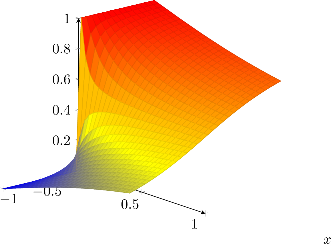
The function \(g_3\) is depicted in Figure 1.
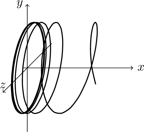
Example 7. The set \[A := \{(x,y,z)\in\mathbb{R}^3:0 < x < 1, y=\sin(1/x), z=\cos(1/x)\} \subseteq \mathbb{R}^3\] depicted in Figure 2 is \(m\)-traceable with fundament \(A_0 =\{*\},A_1=(0,1),A_2=\{(x_1,x_2)\in\mathbb{R}^2:0<x_1<1,x_2=\sin(1/x_1)\},A_3=A\) and signature datum satisfying
\(f_1 = 0,\quad g_1=1\),
\(f_2(x_1) = g_2(x_1) = \sin(1/x_1)\),
\(f_3(x_1,x_2) = g_3(x_1,x_2)=\cos(1/x_1)\).
Let \(A\) be \(m\)-traceable with fundament \(A_0,\ldots,A_n\) and signature datum \((\{f_i,g_i\}_{i\in[n]})\). Then \(A\) is also \(m'\)-traceable for \(m'\leq m\) and each \(A_i\) is \(m'\)-traceable with signature datum \((\{f_1,g_1\}, \ldots, \{f_i,g_i\})\) and fundament \(A_0,\ldots, A_i\) for \(i\in[n]\).
Now fix \(i\in[n]\). Then \(A_i\) is bounded and \[(x_1,\ldots,x_i) \in A_i \iff \bigwedge_{j=1}^i x_j \in (\tilde{f}_j(x_1,\ldots,x_{j-1}),\tilde{g}_j(x_1,\ldots,x_{j-1}))_{\mathbb{R}^0}\] where \(\tilde{f}_j,\tilde{g}_j:\mathbb{R}^{j-1} \to \mathbb{R}_\infty\) extend \(f_j,g_j\) by \(\tilde{f}_j(x_1,\ldots,x_{j-1}):=\infty\) and \(\tilde{g}_j(x_1,\ldots,x_{j-1}) := -\infty\) for \((x_1,\ldots,x_{j-1}) \in \mathbb{R}^{j-1}\setminus A_{j-1}\), \(j\in[i]\).
For \(j\in[i]\), this yields that \(A_j = \pi_i^{\leq j}(A_i)\) and for \(a \in A_j\), \[(x_{j+1},\ldots,x_i) \in A_i(a) \iff \bigwedge_{k=j+1}^i x_k \in (\tilde{f}_k(a,x_{j+1},\ldots,x_{k-1}),\tilde{g}_k(a,x_{j+1},\ldots,x_{k-1}))_{\mathbb{R}^0}.\] So \(A_i(a)\) is also \(m\)-traceable with signature datum \((\{f_{j+1}(a), g_{j+1}(a)\},\ldots, \{f_i(a),g_i(a)\})\) and fundament \(A_j(a), \ldots, A_i(a)\). The fundament and the signature datum of \(A\) are unique.
The next lemma provides a bound on the Lebesgue measure of \(A_i\).
Lemma 5. For each \(i\in[n]\), \(A_i\) is measurable and \[\lambda^i(A_i) \leq \prod_{j=1}^i \norm{g_j-f_j}_{L^\infty(A_{j-1})}\] holds. In particular, if \(f_j = g_j\) for some \(j\in[n]\), then \(\lambda^i(A) = 0\) for \(i\geq j\).
Proof. First, \(A_1\) is measurable and \(\lambda^1(A_1) = \lambda^1((f_1,g _1)_{A_0}) = g_1-f_1 = \norm{g_1-f_1}_{L^\infty(\mathbb{R}^0)}\). Suppose that the claim holds for \(A_1,\ldots,A_i,i<n\). The measurability of \(A_{i+1}\) follows from (the proof of)[12], Lemma A.9. Since \(A_{i+1} = (f_{i+1},g_{i+1})_{A_i}\), Fubini’s theorem gives \[\lambda^{i+1}(A_{i+1})= \int_{A_i} g_{i+1}(x)-f_{i+1}(x) dx \leq \lambda^i(A_i)\norm{g_{i+1}-f_{i+1}}_{L^\infty(A_i)} \leq \prod_{j=1}^{i+1} \norm{g_j-f_j}_{L^\infty(A_{j-1})}.\] The second claim follows. ◻
Corollary 3. For each \(i\in[n]\), \(a \in A_j\), \(j<i\), we have that \[\lambda^{i-j}(A_i(a)) \leq \prod_{k=j+1}^i \norm{g_k(a)-f_k(a)}_{L^\infty(A_{k-1}(a))}.\] Furthermore, if \(f_k(a) = g_k(a)\) for some \(j<k\leq i\), then \(\lambda^{i-j}(A_i(a)) = 0\).
Proof. Follows from Lemma 5 applied to the \(m\)-traceable set \(A_i(a)\) with signature datum \[(\{f_{j+1}(a), g_{j+1}(a)\},\ldots, \{f_i(a),g_i(a)\}).\] ◻
Definition 12. Define the extended signature datum of \(A\) by \((\{\underline{f}_i,\overline{g}_i\}_{i\in[n]})\) where \(\underline{f}_i\) is the lsc envelope of \(f_i\) and \(\overline{g}_i\) is the usc envelope of \(g_i\) for each \(i\in[n]\). For \(m'\leq m\), we say that \(A\) is \(m'\)-extendable if for every \(i\in[n]\), \(\underline{f}_i|_{\mathop{\mathrm{cl}}(A_{i-1})}\) and \(\overline{g}_i|_{\mathop{\mathrm{cl}}(A_{i-1})}\) are \(C^{m'}\). If \(A \subseteq Q_n\) and each \(f_i,g_i\) is the restriction of \(C^m\) functions \(F_i, G_i:Q_{i-1} \to \mathbb{R}\) with \(\norm{F_i}_{W^{m,\infty}(Q_{i-1})} \leq B\) and \(\norm{G_i}_{W^{m,\infty}(Q_{i-1})} \leq B\) for each \(i\in[n]\), we say that \(A\) has the \((m,B)\)-extension property.
With the extended signature datum of \(A\), an explicit description of its topological closure \(\mathop{\mathrm{cl}}(A)\) is possible.
Lemma 6. For each \(i \in [n]\), we have \[\mathop{\mathrm{cl}}(A_i) \subseteq \{(x_1,\ldots,x_i) \in \mathbb{R}^i: \underline{f}_1 \leq x_1 \leq \overline{g}_1, \ldots, \underline{f}_i(x_1,\ldots,x_{i-1}) \leq x_i \leq \overline{g}_i(x_1,\ldots,x_{i-1})\}.\] Moreover, if \(A\) is \(1\)-extendable, then equality holds.
Proof. Considering \(A_1=(f_1,g_1)_{A_0}\), we see that \(\mathop{\mathrm{cl}}(A_1)=\{x_1\in\mathbb{R}:f_1\leq x_1\leq g_1\}=\{x_1\in\mathbb{R}:\underline{f}_1\leq x_1\leq \overline{g}_1\}\).
Suppose the statement holds for \(A_1,\ldots,A_i\), \(i<n\). It is enough to show that \(\mathop{\mathrm{cl}}(A_{i+1}) \subseteq \Gamma^\uparrow(\underline{f}_{i+1}) \cap \Gamma^\downarrow(\overline{g}_{i+1})\) since by assumption \[\begin{align} \mathop{\mathrm{dom}}(\underline{f}_{i+1}) = \mathop{\mathrm{dom}}(\overline{g}_{i+1})=\mathop{\mathrm{cl}}(A_i) \subseteq \{ & (x_1,\ldots,x_i) \in \mathbb{R}^i: \quad \underline{f}_1 \leq x_1 \leq \overline{g}_1, \ldots, \\ & \underline{f}_i(x_1,\ldots,x_{i-1}) \leq x_i \leq \overline{g}_i(x_1,\ldots,x_{i-1})\} \end{align}\] and \(\Gamma^\uparrow(\underline{f}_{i+1}),\Gamma^\downarrow(\overline{g}_{i+1}) \subseteq \mathop{\mathrm{cl}}(A_i) \times \mathbb{R}\) by Lemma 2. Since \(A_{i+1} \subseteq \Gamma^\uparrow(\underline{f}_{i+1})\cap\Gamma^\downarrow(\overline{g}_{i+1})\) and \(\Gamma^\uparrow(\underline{f}_{i+1})\cap\Gamma^\downarrow(\overline{g}_{i+1})\) is closed by Proposition 4, we get that \(\mathop{\mathrm{cl}}(A_{i+1}) \subseteq \Gamma^\uparrow(\underline{f}_{i+1})\cap\Gamma^\downarrow(\overline{g}_{i+1})\).
For the second part, assume that \(A\) is \(1\)-extendable and that equality holds for \(A_1,\ldots,A_i\), \(i<n\). Suppose that \((x_1,\ldots,x_{i+1}) \in \mathbb{R}^{i+1}\) satisfies \[\underline{f}_1 \leq x_1 \leq \overline{g}_1, \ldots, \underline{f}_{i+1}(x_1,\ldots,x_i) \leq x_{i+1} \leq \overline{g}_{i+1}(x_1,\ldots,x_i).\] Then \((x_1,\ldots,x_i) \in \mathop{\mathrm{cl}}(A_i)\) and it remains to show that \(U_\delta \cap A_{i+1} \neq \emptyset\) for every open box \(U_\delta:= \bigtimes_{j=1}^{i+1} (x_j-\delta,x_j+\delta)\) around \((x_1,\ldots,x_{i+1})\). Note that \(\pi_{i+1}(U_\delta) = \bigtimes_{j=1}^i (x_j-\delta,x_j+\delta)\) and \(\pi_{i+1}(U_\delta) \cap A_i \neq \emptyset\). Since \(A\) is \(1\)-extendable, \(\underline{f}_{i+1}|_{\mathop{\mathrm{cl}}(A_i)}\) and \(\overline{g}_{i+1}|_{\mathop{\mathrm{cl}}(A_i)}\) are continuous. So for any \(\varepsilon > 0\), there is \(\delta>0\) with \[f_{i+1}(\pi_{i+1}(U_\delta) \cap A_i) \subseteq (\underline{f}_{i+1}(x_1,\ldots,x_i)-\varepsilon, \underline{f}_{i+1}(x_1,\ldots,x_i)+\varepsilon)\] and \[g_{i+1}(\pi_{i+1}(U_\delta)\cap A_i) \subseteq (\overline{g}_{i+1}(x_1,\ldots,x_i)-\varepsilon, \overline{g}_{i+1}(x_1,\ldots,x_i)+\varepsilon).\] We distinguish three cases.
Case 1. \(\varepsilon_1 := x_{i+1} - \underline{f}_{i+1}(x_1,\ldots,x_i) >0\) and \(\varepsilon_2 := \overline{g}_{i+1}(x_1,\ldots,x_i) - x_{i+1} > 0\).
Here, there is some \(\delta > 0\) such that \[f_{i+1}(\pi_{i+1}(U_\delta) \cap A_i) \subseteq (\underline{f}_{i+1}(x_1,\ldots,x_i)-\varepsilon_1, \underline{f}_{i+1}(x_1,\ldots,x_i)+\varepsilon_1) \subseteq (-\infty, x_{i+1})\] and \[g_{i+1}(\pi_{i+1}(U_\delta)\cap A_i) \subseteq (\overline{g}_{i+1}(x_1,\ldots,x_i)-\varepsilon_2, \overline{g}_{i+1}(x_1,\ldots,x_i)+\varepsilon_2) \subseteq (x_{i+1},\infty).\] In particular, if \((x_1',\ldots,x_i') \in \pi_{i+1}(U_\delta)\cap A_i\), then \(f_{i+1}(x_1',\ldots,x_i') < x_{i+1} < g_{i+1}(x_1',\ldots,x_i')\), so \((x_1',\ldots,x_i',x_{i+1}) \in U_\delta \cap A_{i+1}\).
Case 2. \(\varepsilon_1 = 0\).
Take any \((x_1',\ldots,x_i') \in \pi_{i+1}(U_\delta)\cap A_i\) such that \(f_{i+1}(x_1',\ldots,x_i') \in (x_{i+1}-\delta/2, x_{i+1}+\delta/2)\) and define \[x_{i+1}' := f_{i+1}(x_1',\ldots,x_i') + \min \{ \delta,g_{i+1}(x_1',\ldots,x_i') - f_{i+1}(x_1',\ldots,x_i') \}/2.\] Then \((x_1',\ldots,x_{i+1}') \in U_\delta \cap A_{i+1}\).
Case 3. \(\varepsilon_2=0 \neq \varepsilon_1\).
Take any \((x_1',\ldots,x_i') \in \pi_{i+1}(U_\delta)\cap A_i\) such that \(g_{i+1}(x_1',\ldots,x_i') \in (x_{i+1}-\delta/2, x_{i+1}+\delta/2)\) and define \[x_{i+1}' := g_{i+1}(x_1',\ldots,x_i') - \min \{ \delta,g_{i+1}(x_1',\ldots,x_i') - f_{i+1}(x_1',\ldots,x_i') \}/2.\] Then \((x_1',\ldots,x_{i+1}') \in U_\delta \cap A_{i+1}\). ◻
If \(A\) is not \(m\)-extendable, then the second conclusion of Lemma 6 might or might not fail as the revisited examples show.
Example 8. Let \(A\) be as in example 6. Then \(A\) is not \(m\)-extendable since at \(x_1=x_2=0\), there is no continuous extension of \(g_3\) to the closure of its domain, as depicted in Figure 1.
Example 9. The set \(A\) as in example 7 is not \(m\)-extendable. The lsc extension of \(f_2\) and the usc extension of \(g_2\) are given by \(\underline{f}(0)= -1\) and \(\overline{g}(0) = 1\). The lsc extension of \(f_3\) and the usc extension of \(g_3\) are given by \(\underline{f}_3(0,x_2) = -\sqrt{1-x_2^2}\) and \(\overline{g}_3(0,x_2) = \sqrt{1-x_2^2}\) for \(x_2 \in [-1,1]\). Since \(\mathop{\mathrm{cl}}(A) = A \cup \{(0,x_2,x_3):x_2^2+x_3^2=1\} \cup \{(1,\sin(1),\cos(1))\}\) does not include the filled circle \(\{(0,x_2,x_3):x_2^2+x_3^2\leq 1\}\), the second conclusion of Lemma 6 fails, see Figure 2.
Using the description of \(\mathop{\mathrm{cl}}(A)\) from Lemma 6 allows to explicitly analyze the frontier of \(A\).
Corollary 4. The frontier of \(A\) is contained in a union of \(2n\) (not necessarily distinct or non-empty) sets \[\begin{align} \mathop{\mathrm{fr}}(A) & \subseteq \{\underline{f}_1 = x_1 \leq \overline{g}_1, \ldots, \underline{f}_n(x_1,\ldots,x_{n-1})\leq x_n \leq \overline{g}_n(x_1,\ldots,x_{n-1})\} \\ & \cup \{\underline{f}_1 \leq x_1 = \overline{g}_1, \ldots, \underline{f}_n(x_1,\ldots,x_{n-1})\leq x_n \leq \overline{g}_n(x_1,\ldots,x_{n-1})\} \\ & \cup \ldots \\ & \cup \{\underline{f}_1 \leq x_1 \leq \overline{g}_1, \ldots, \underline{f}_n(x_1,\ldots,x_{n-1}) = x_n \leq \overline{g}_n(x_1,\ldots,x_{n-1})\} \\ & \cup \{\underline{f}_1 \leq x_1 \leq \overline{g}_1, \ldots, \underline{f}_n(x_1,\ldots,x_{n-1})\leq x_n = \overline{g}_n(x_1,\ldots,x_{n-1})\} \end{align}\] where in each of the \(2n\) sets exactly one equality occurs. If \(A\) is \(1\)-extendable, then \(\lambda^n(\mathop{\mathrm{fr}}(A))= 0\).
Proof. For \(x \in \mathop{\mathrm{fr}}(A)\), let \(i \in [n]\) be minimal such that \[f_i(x_1,\ldots,x_{i-1}) < x_i < g_i(x_1,\ldots,x_{i-1})\] does not hold. By minimality of \(i\), \((x_1,\ldots,x_{i-1}) \in \mathop{\mathrm{dom}}(f_i) = \mathop{\mathrm{dom}}(g_i)\). As \(\underline{f}_i(x_1,\ldots,x_{i-1}) \leq x_i \leq \overline{g}_i(x_1,\ldots,x_{i-1})\) and \(\pi_n^{<i}(x) \in A_{i-1}\), \(\underline{f}_i(x_1,\ldots,x_{i-1}) = x_i\) or \(x_i = \overline{g}_i(x_1,\ldots,x_{i-1})\) must be true.
For the second part, we show that the right hand side is a null-set. Assume that \(A\) is \(1\)-extendable. Applying the Whitney extension theorem [29] to \(\underline{f}_i|_{\mathop{\mathrm{cl}}(A_{i-1})}\) and \(\overline{g}_i|_{\mathop{\mathrm{cl}}(A_{i-1})}\) yields the existence of global \(C^m\) extensions \(F_i:\mathbb{R}^{i-1} \to \mathbb{R}\) of \(\underline{f}_i|_{\mathop{\mathrm{cl}}(A_{i-1})}\) and \(G_i:\mathbb{R}^{i-1}\to\mathbb{R}\) of \(\overline{g}_i|_{\mathop{\mathrm{cl}}(A_{i-1})}\) for each \(i \in [n]\). Then \(\Gamma(F_i) \times \mathbb{R}^{n-i}\) and \(\Gamma(G_i) \times \mathbb{R}^{n-i}\), whose union over \(i\in[n]\) contains \(\mathop{\mathrm{fr}}(A)\), are \(C^m\) submanifolds of \(\mathbb{R}^n\) of dimension \(n-1\), given as the zero sets of the global \(C^m\) submersions \(\mathbb{R}^n \to \mathbb{R}\), \(x \mapsto x_i - F_i(x_1,\ldots,x_{i-1})\) and \(x \mapsto G_i(x_1,\ldots,x_{i-1}) - x_i\). As finite unions of \(C^m\) submanifolds of \(\mathbb{R}^n\) of dimension less than \(n\) are null-sets [30], the statement follows. ◻
Assume that \(A \subseteq Q_n\) is \(m\)-extendable. We associate to \(A\) the constant \[B_A^m := \inf \max_{j\in[n]} \{\max_{\abs{\alpha}\leq m} \norm{\partial^\alpha F_j}_{L^\infty Q_{j-1}}, \max_{\abs{\alpha}\leq m} \norm{\partial^\alpha G_j}_{L^\infty Q_{j-1}} \}\] where for \(i\in[n]\), \(F_i\) and \(G_i\) range over all \(C^m\) functions \(Q_{i-1} \to \mathbb{R}\) extending \(f_i\) and \(g_i\) respectively. Recall that \(\mathcal{K}_{m,n}^B\) is the set of all \(m\)-traceable subsets of \(Q_n\) with the \((m,B)\)-extension property and that \(\mathcal{K}_{m,n}^{B,\ell}\) is the set of all \((m,\ell)\)-traceable subsets of \(Q_n\) with the \((m,B,\ell)\)-extension property. Note that \(\mathcal{K}_{m,n}^{B,\ell'} \subseteq \mathcal{K}_{m,n}^{B,\ell}\) for \(\ell' \leq \ell\). Let \(\Omega \subseteq \mathbb{R}^n\) be \((m,\ell)\)-traceable. Then \(\Omega = A^1 \cup \cdots \cup A^l\) for some \(l \leq \ell\) and pairwise disjoint \(m\)-traceable \(A^j\) for \(j\in[l]\). If \(l\) and \(A^j\) can be chosen so that \(A^j\) is \(m\)-extendable for every \(j\in[l]\), then \(\Omega\) is said to be \((m,\ell)\)-extendable. Assume that \(\Omega \subseteq Q_n\) is \((m,\ell)\)-extendable. Associate to \(\Omega\) the constant \[B_\Omega^m := \inf\{\max_{j\in[l]} B_{A^j}^m: \quad \Omega = A^1\cup\cdots\cup A^l,l\leq\ell, A^j \in \bigcup_{B>0}\mathcal{K}_{m,n}^B \text{ pairwise disjoint}\}.\] This definition is consistent with \(\mathcal{K}_{m,n}^B \subseteq \mathcal{K}_{m,n}^{B,\ell}\)for \(\ell \geq 1\).
Lemma 7. The following statements hold.
For every \(B > B_A^m\), we have that \(A \in \mathcal{K}_{m,n}^B\).
For every \(B > B_\Omega^m\), we have that \(\Omega \in \mathcal{K}_{m,n}^{B,\ell}\).
Proof. (i) Since \(A\) is \(m\)-extendable, it follows for each \(i \in [n]\), that \(\underline{f}_i|_{\mathop{\mathrm{cl}}(A_{i-1})}\) and \(\overline{g}_i|_{\mathop{\mathrm{cl}}(A_{i-1})}\) are \(C^m\) and by the Whitney extension theorem [29], there are global \(C^m\) extensions \(F_i:\mathbb{R}^{i-1} \to \mathbb{R}\) of \(\underline{f}_i|_{\mathop{\mathrm{cl}}(A_{i-1})}\) and \(G_i:\mathbb{R}^{i-1}\to\mathbb{R}\) of \(\overline{g}_i|_{\mathop{\mathrm{cl}}(A_{i-1})}\). Restricting \(F_i\) and \(G_i\) to \(Q_{i-1}\) yields a bound on their Sobolev norms since the continuous functions \(\abs{\partial^\alpha F_i},\abs{\partial^\alpha G_i}:Q_{i-1} \to \mathbb{R}\) attain their maximal values on their compact domains. By definition of \(B_A^m\), it is possible to choose \(F_i\) and \(G_i\) in a way such that \[B_A^m < \max \{ \norm{F_i}_{W^{m,\infty}(Q_{i-1})}, \norm{G_i}_{W^{m,\infty}(Q_{i-1})}\} < B.\] So \(A\) has the \((m,B)\)-extension property.
(ii) By (i) and the definition of \(B_\Omega^m\), we get that for any \(B > B_\Omega^m\), there are \(A^1,\ldots,A^l \in \mathcal{K}_{m,n}^B\) such that \(\Omega = A^1\cup\cdots\cup A^l\), so \(\Omega \in \mathcal{K}_{m,n}^{B,\ell}\). ◻
We study parametric collections coming from fibers of elements of \(\mathcal{K}_{m,k+n}^{B,\ell}\).
Lemma 8. Let \(\Omega \in \mathcal{K}_{m,k+n}^{B,\ell}\). Then \(\Omega(a) \in \mathcal{K}_{m,n}^{B,\ell}\) for each \(a\in Q_k\).
Proof. By assumption, there are pairwise disjoint \(A^1,\ldots,A^l \in \mathcal{K}_{m,k+n}^B\), \(l\leq \ell\), such that \(\Omega = A^1\cup\cdots\cup A^l\). Then \(\Omega(a) = A^1(a) \cup \cdots \cup A^l(a)\). For \(i \in [l]\), let \((\{f^i_j,g^i_j\}_{j\in[k+n]})\) be the signature datum of \(A^i\). For each \(j\in[k+n]\), there are \(C^m\) maps \(F_j^i,G_j^i:Q_{j-1}\to\mathbb{R}\) extending \(f_j^i\) and \(g_j^i\) respectively such that \[\max_{j\in[k+n]}\max\{\norm{F_j^i}_{W^{m,\infty}(Q_{j-1})},\norm{G_j^i}_{W^{m,\infty}(Q_{j-1})}\}\leq B.\] Then, for \(j>k\), the maps \(F_j^i(a)\) and \(G_j^i(a)\) extending \(f_j^i(a)\) and \(g_j^i(a)\) satisfy \[\max_{j>k}\max\{\norm{F_j^i(a)}_{W^{m,\infty}(Q_{j-1-k})},\norm{G_j^i(a)}_{W^{m,\infty}(Q_{j-1-k})}\}\leq B,\] invoking Lemma 1. Since \((\{f_j^i(a),g_j^i(a)\}_{j>k})\) is the signature datum of \(A^i(a)\), we get \(A^i(a) \in \mathcal{K}_{m,n}^B\). Hence \(A^i(a) \in \mathcal{K}_{m,n}^B\) for every \(i\in[l]\), so \(\Omega(a) \in \mathcal{K}_{m,n}^{B,\ell}\). ◻
6.1 The property of being extendable↩︎
In general, derivatives of bounded functions on open domains can be uncontrollable towards the boundary, hence not every \((m,\ell)\)-traceable subset of \(Q_n\) is \((m,\ell)\)-extendable. But we expect that every \((m,\ell)\)-traceable subset of \(Q_n\) is relatively close to being \((m,\ell)\)-extendable by infinitesimal shrinking.
Lemma 9. Let \(\ell \in \mathbb{N}\) and \(\Omega \subseteq Q_n\) be an \((m,\ell)\)-traceable set. For every \(\varepsilon > 0\), there is an \((m,\ell)\)-traceable set \(\Omega'\subseteq \Omega\) with the \((m,B,\ell)\)-extension property for some \(B=B(\varepsilon)>0\) such that \[\lambda^n(\Omega \setminus \Omega') \leq \varepsilon.\]
Proof. Let \(\varepsilon > 0\) and pairwise disjoint \(m\)-traceable sets \(A^1,\ldots,A^l\), \(l\leq \ell\) with fundaments \(A_0^j,\ldots,A_n^j\) and signature data \((\{f_i^j,g_i^j\}_{i\in[n]})\) for \(j\in[l]\) be given such that \(\Omega=A^1\cup\cdots\cup A^l\). We show that there is some \(B>0\) and \(m\)-traceable sets \((A^j)'\subseteq A^j\), \(j\in[l]\) such that \((A^j)'\) is \((m,B)\)-extendable and \(\Omega' = (A^1)'\cup\cdots\cup (A^l)'\) satisfies the conclusion of the Lemma.
Fix \(j\in[l]\). If there is some \(i\in[n]\) such that \(f_i^j = g_i^j\), then Lemma 5 yields that \(\lambda^n(A^j) = 0\) and we can take \((A^j)' := \{x\}\) for any \(x \in A^j\). Then the extended signature datum of \((A^j)'\) is equal to the signature datum of \(\{x\}\) as in Example 5.
For notational convenience, we set \(f_i:=f_i^j\) and \(g_i:=g_i^j\) for \(i\in[n]\), and \(A:=A^j\). Suppose that \(f_i<g_i\) for all \(i\in[n]\). For \(0 < \delta < 1/2\) and \(i\in[n]\), define \(f^\delta_i, g^\delta_i: A_{i-1} \to \mathbb{R}\) by \[f^\delta_i(x) :=(1-\delta)f_i(x)+\delta g_i(x)\] and \[g^\delta_i(x) := \delta f_i(x) + (1-\delta)g_i(x).\] Then \(f_i < f^\delta_i < g^\delta_i < g_i\) and recursively setting \(A_i^\delta := (f^\delta_i|_{A_{i-1}^\delta},g^\delta_i|_{A_{i-1}^\delta})_{A_{i-1}^\delta}\) for \(i\in[n]\) with \(A_0^\delta = A_0\) yields the \(m\)-traceable set \(A^\delta := A_n^\delta\) with signature datum \((\{f_1^\delta|_{\mathbb{R}^0},g_1^\delta|_{\mathbb{R}^0}\},\ldots,\{f_n^\delta|_{A_{n-1}^\delta},g_n^\delta|_{A_{n-1}^\delta}\})\). Since \(\mathop{\mathrm{cl}}(A_i^\delta)\) is a compact subset of \(A_i\) for each \(i\in[n]\), the functions \(\underline{f}_i^\delta|_{\mathop{\mathrm{cl}}(A_i^\delta)}\) and \(\overline{g}_i^\delta|_{\mathop{\mathrm{cl}}(A_i^\delta)}\) are \(C^m\), witnessed by their \(C^m\) extensions \(f_i^\delta\) and \(g_i^\delta\) to an open neighborhood of \(\mathop{\mathrm{cl}}(A_i^\delta)\) contained in \(A_i\). Thus \(A^\delta\) is \(m\)-extendable and by the Whitney extension theorem, there exist \(C^m\) maps \(F_i^\delta,G_i^\delta: Q_{i-1} \to \mathbb{R}\) such that \(F_i^\delta|_{\mathop{\mathrm{cl}}(A_i^\delta)}=\underline{f}_i^\delta|_{\mathop{\mathrm{cl}}(A_i^\delta)}\) and \(G_i^\delta|_{\mathop{\mathrm{cl}}(A_i^\delta)}=\overline{g}_i^\delta|_{\mathop{\mathrm{cl}}(A_i^\delta)}\). It follows from Lemma 7 that \(A^\delta\) has the \((m,B)\)-extension property for \[B:=\max_{j\in[n]} \{\norm{F_j^\delta}_{W^{m,\infty}Q_{j-1}}, \norm{G_j^\delta}_{W^{m,\infty}Q_{j-1}} \}.\] Note that \[\norm{f^\delta_i-f_i}_{L^\infty(A_{i-1})} = \norm{g_i-g^\delta_i}_{L^\infty(A_{i-1})} = \delta \norm{g_i-f_i}_{L^\infty(A_{i-1})}.\] Applying Lemma 5 to \(A_i^\delta\) yields \[\lambda^i(A_i^\delta) \leq \prod_{j=1}^i \norm{g_j^\delta-f_j^\delta}_{L^\infty(A^\delta_{j-1})} \leq \prod_{j=1}^i \norm{g_j-f_j}_{L^\infty(A^\delta_{j-1})}\] For \(A_1 = (f_1,g_1)_{A_0}\) we explicitly have \[\lambda^1(A_1\setminus A_1^\delta) = \lambda^1((f_1,(1-\delta)f_1+\delta g_1)_{A_0} \cup (\delta f_1 + (1-\delta)g_1,g_1)_{A_0})= 2\delta (g_1 - f_1).\] Next, if \((x_1,\ldots,x_{i+1}) \in A_{i+1} \setminus A_{i+1}^\delta\) for \(i \in [n]\), then \((x_1,\ldots,x_i) \in A_i\setminus A_i^\delta\) and \[f_{i+1}(x_1,\ldots,x_i) < x_{i+1} < g_{i+1}(x_1,\ldots,x_i),\] or \((x_1,\ldots,x_i) \in A_i^\delta\) and \(x_{i+1} \in (f_{i+1}, f^\delta_{i+1}) \cup (g^\delta_{i+1}, g_{i+1})\). So \[\begin{align} \lambda^{i+1}(A_{i+1} \setminus A_{i+1}^\delta) & \leq \lambda^i(A_i\setminus A_i^\delta)\norm{g_{i+1}-f_{i+1}}_{L^\infty(A_i\setminus A_i^\delta)}\\ & + \lambda^i(A_i^\delta) \norm{g_{i+1}-g^\delta_{i+1}}_{L^\infty(A_i^\delta)} \\ & + \lambda^i(A_i^\delta) \norm{f^\delta_{i+1}-f_{i+1}}_{L^\infty(A_i^\delta)} \\ & \leq \lambda^i(A_i\setminus A_i^\delta)\norm{g_{i+1}-f_{i+1}}_{L^\infty(A_i)}\\ & + 2\lambda^i(A_i^\delta) \delta\norm{g_{i+1}-f_{i+1}}_{L^\infty(A_i)} \\ & \leq \lambda^i(A_i\setminus A_i^\delta)\norm{g_{i+1}-f_{i+1}}_{L^\infty(A_i)} \\ & +2\delta\prod_{j=1}^{i+1}\norm{g_j-f_j}_{L^\infty(A_{j-1})}, \end{align}\] using Lemma 5 for the last inequality. A discrete version of Grönwall’s inequality implies that \[\lambda^n(A\setminus A^\delta) \leq 2n\delta \prod_{j=1}^n\norm{g_j-f_j}_{L^\infty(A_{j-1})} \leq \varepsilon/\ell\] by recursively plugging in bounds for \(\lambda^i(A_i\setminus A_i^\delta)\) and taking \(\delta \leq \varepsilon/2n\ell\prod_{j=1}^n\norm{g_j-f_j}_{L^\infty(A_{j-1})}\). Setting \((A^j)' := A^\delta\) yields \[\lambda^n(\Omega\setminus\Omega') = \sum_{j=1}^l\lambda(A^j\setminus (A^j)') \leq \ell \max_j \lambda(A^j\setminus (A^j)') \leq \ell \varepsilon/\ell = \varepsilon,\] showing the claim. ◻
6.2 Connection between traceable and definable sets↩︎
The next lemma connects traceable sets with definable sets.
Lemma 10. Every (bounded) \((i_1,\ldots,i_n)\)-\(C^m\)-cell \(C \subseteq \mathbb{R}^n\) is \(m\)-traceable with fundament \(C_i=\pi^{\leq i}_n(C)\). Moreover, every bounded definable set \(A \subseteq \mathbb{R}^n\) is \((m,\ell)\)-traceable for some \(\ell \geq 0\) and for every definable collection \(\{A(a):a \in \mathbb{R}^i\} \subseteq \mathcal{P}(\mathbb{R}^{n-i})\) there is some \(\ell \geq 0\) such that \(A(a)\) is \((m,\ell)\)-traceable for all \(a \in \mathbb{R}^i\).
Proof. By induction on \(n\). For \(n=0\) and \(n=1\), this is clear. Let \(C\) be an \((i_1,\ldots,i_n)\)-\(C^m\)-cell and assume bounded, definably \(C^m\) functions \(f,g:C\to\mathbb{R}\) with either \(f=g\) or \(f<g\) are given. Then \(f\) and \(g\) are in particular \(C^m\). Inductively, \(C\) is \(m\)-traceable with signature datum \((\{f_i,g_i\}_{i\in[n]})\) and fundament \(C_0,\ldots,C_n\). Then \((f,g)_C\) has signature datum \((\{f_i,g_i\}_{i\in[n]},\{f,g\})\) and fundament \(C_0,\ldots,C_n,(f,g)_C\). By Theorem 7, every definable set is the disjoint union of finitely many \(C^m\)-cells. Lemma 4 yields that the number of \(C^m\)-cells needed to decompose fibers of definable sets is uniformly bounded. ◻
The following corollary collects the properties of the rectangular shape of \(C^m\)-cells that were derived for \(m\)-traceable sets in Section 6.
Corollary 5. Let \(C \subseteq \mathbb{R}^n\) be a \(C^m\)-cell viewed as an \(m\)-traceable set with fundament \(C_0,\ldots,C_n\) and signature datum \((\{f_1,g_1\}, \ldots, \{f_n,g_n\})\). Then for each \(i<n\),
\(C_i\) is a \(C^m\)-cell with fundament \(C_0,\ldots,C_i\) and signature datum \((\{f_1,g_1\}, \ldots, \{f_i,g_i\})\),
\(C_j = \pi_i^{\leq j}(C_i)\) and \(C_j(x)=\pi_i^{\leq j}(C_i(x))\) for \(j < i\),
For \(x \in C_i\), the fiber \(C(x)\) above \(x\) is a \(C^m\)-cell with signature datum \[(\{f_{i+1}(x),g_{i+1}(x)\}, \ldots, \{f_n(x),g_n(x)\}),\]
Further, suppose that \(C\) is \(1\)-extendable. Then
The closure of \(C\) can be described by \[\begin{align} \mathop{\mathrm{cl}}(C) = \{ & (x_1,\ldots,x_n)\in\mathbb{R}^n: \underline{f}_1 \leq x_1 \leq \overline{g}_1, \ldots, \\ &\underline{f}_n(x_1,\ldots,x_{n-1}) \leq x_n \leq \overline{g}_n(x_1,\ldots,x_{n-1})\}, \end{align}\]
The frontier of \(C\) is \[\begin{align} \mathop{\mathrm{fr}}(C) \subseteq & \{\underline{f}_1 = x_1 \leq \overline{g}_1, \ldots, \underline{f}_n(x_1,\ldots,x_{n-1})\leq x_n \leq \overline{g}_n(x_1,\ldots,x_{n-1})\} \\ & \cup \{\underline{f}_1 \leq x_1 = \overline{g}_1, \ldots, \underline{f}_n(x_1,\ldots,x_{n-1})\leq x_n \leq \overline{g}_n(x_1,\ldots,x_{n-1})\} \\ & \cup \ldots \\ & \cup \{\underline{f}_1 \leq x_1 \leq \overline{g}_1, \ldots, \underline{f}_n(x_1,\ldots,x_{n-1}) = x_n \leq \overline{g}_n(x_1,\ldots,x_{n-1})\} \\ & \cup \{\underline{f}_1 \leq x_1 \leq \overline{g}_1, \ldots, \underline{f}_n(x_1,\ldots,x_{n-1})\leq x_n = \overline{g}_n(x_1,\ldots,x_{n-1})\} \end{align}\] where equality holds if \(f_i<g_i\) for all \(i\in[n]\).
If \(C \subseteq Q_n\), then \(C \in \mathcal{K}_{m,n}^B\) for each \(B>B_C^m\).
Lemma 9 implies that sets with the extension property are ‘dense’ among definable subsets of \(Q_n\):
Corollary 6. Let \(A\subseteq Q_n\) be a definable set. For every \(\varepsilon>0\), there is some definable set \(A'\subseteq A\) such that \(A'\in\mathcal{K}_{m,n}^{B,\ell}\) for some \(B>0\), \(\ell \in \mathbb{N}\) with \[\lambda^n(A \setminus A') \leq \varepsilon.\]
Proof. By Lemma 10, every definable set is \((m,\ell)\)-traceable for some \(\ell \in \mathbb{N}\). Applying Lemma 9 and following the definable construction of \(A'\) in its proof yields the claim. ◻
Call a definable set \(\Omega\subseteq Q_n\) \(m\)-admissible if \(\Omega\) has a \(C^m\)-cell decomposition \(\mathcal{C} \subseteq \mathcal{K}_{m,n}\) viewing each \(C \in \mathcal{C}\) as an \(m\)-traceable set.
Assume that \(\Omega\) is \((m,\ell)\)-traceable and \(m\)-admissible. By Lemma 7, \(\Omega\in\mathcal{K}_{m,n}^{B,\ell}\) for \(B>B_\Omega^m\) viewing \(\Omega\) as an \((m,\ell)\)-traceable set. The next corollary ensures that all fibers of \(\Omega\) have the \((m,B)\)-extension property, giving a useful generation procedure of subclasses of \(\mathcal{K}_{m,n-i}^{B,\ell}\) via definable collections.
Lemma 11. Let \(i<n\) and \(\mathcal{A}_{i,D}\) be the definable collection coming from \(\Omega\) with parameter space \(D = Q_i\) and \(B > B_\Omega^m\). Then \(\Omega(a) \in \mathcal{K}_{m,n-i}^{B,\ell}\) for all \(a \in D\).
Proof. Analogous to the proof of Lemma 8, using that \(\Omega\in\mathcal{K}_{m,n}^{B,\ell}\) for \(B>B_\Omega^m\). ◻
7 ReLU neural network approximation of traceable sets↩︎
Most of this section is based on [2] and [19]. We first adapt the function classes from [2] to our setting and ensure they can still be approximated by controllable classes of ReLU neural networks. With these function classes, we build approximating ReLU neural networks for characteristic functions of traceable sets, keeping track of the architecture and the approximation error. We let \(H_i: \mathbb{R}^n \to \mathbb{R}\), \(H_i := \chi_{\mathbb{R}^{i-1} \times [0,\infty) \times \mathbb{R}^{n-i}}\) for \(i\in[n]\).
Definition 13. For \(B>0\), define the set of functions \[\mathcal{F}_{m,n}^B:=\{ f \in C^m(Q_n):\norm{f}_{W^{m,\infty}(Q_n)} \leq B\}.\] Further, for \(n \geq 2\), let the horizon functions with respect to \(\mathcal{F}_{m,n}^B\) be given by \[\mathcal{HF}_{m,n}^B:=\mathcal{HF}_{m,n}^{B,+} \cup \mathcal{HF}_{m,n}^{B,-}\] where \[\mathcal{HF}_{m,n}^{B,+}:=\bigcup_{i=1}^n\{f\in L^{\infty}(Q_n):f(x)=H_i(x-e_i\gamma(x^{<i})):\gamma \in \mathcal{F}_{m,i-1}^B\}\] and \[\mathcal{HF}_{m,n}^{B,-}:=\bigcup_{i=1}^n\{f\in L^{\infty}(Q_n):f(x)=H_i(e_i\gamma(x^{<i})-x):\gamma \in \mathcal{F}_{m,i-1}^B\}\] abbreviating \(x^{< i} := (x_1,\ldots,x_{i-1})\).
For every \(f \in \mathcal{F}_{m,n}^B\), we have that \(-f \in \mathcal{F}_{m,n}^B\) and \(\norm{\partial^\alpha f}_{L^\infty(Q_n)} \leq B\) for \(\alpha \in \mathbb{N}^n,\abs{\alpha} \leq m\). So for \(\abs{\alpha} = m-1\) we get \[\abs{\partial^{\alpha} f(x) - \partial^{\alpha} f(y)} \leq \norm{\sqrt{\sum_{i=1}^n (\partial^{\alpha+e_i} f)^2}}_{L^\infty(Q_n)}\norm{x-y} \leq \sqrt{n}B\norm{x-y}.\] Hence \(\mathcal{F}_{m,n}^B \subseteq \mathcal{F}_{\beta,n,\sqrt{n}B}\) for \(\beta = (m-1)+\sigma\) with \(\sigma = 1\), where \(\mathcal{F}_{\beta,n,\sqrt{n}B}\) is defined in [2], (3.1). Thus all approximation results concerning \(\mathcal{F}_{\beta,n,\sqrt{n}B}\) apply to \(\mathcal{F}_{m,n}^B\). Identifying every \(f \in \mathcal{F}_{m,i-1}^B\) with a function \(\gamma_f:Q_{n-1} \to \mathbb{R}\), \((x_1,\ldots,x_{n-1}) \mapsto f(x_1,\ldots,x_{i-1})\) yields the inclusion \(\mathcal{F}_{m,i-1}^B \subseteq \mathcal{F}_{m,n-1}^B\) for each \(i\in[n]\). This follows because \(\norm{\partial^\alpha \gamma_f}_{L^\infty(Q_{n-1})} = 0\) if \(\alpha_j > 0\) for some \(j \geq i\).
Using \(\mathcal{F}_{m,i-1}^B \subseteq \mathcal{F}_{m,n-1}^B \subseteq \mathcal{F}_{\beta,n-1,\sqrt{n}B}\) for \(i \leq n\) yields that \(\mathcal{HF}_{m,n}^{B,+} \subseteq \mathcal{HF}_{\beta,n,\sqrt{n}B}\) for \(\beta = (m-1)+\sigma\) and \(\sigma = 1\), where \(\mathcal{HF}_{\beta,n,\sqrt{n}B}\) is defined in [2], (3.3). But \(\mathcal{HF}_{\beta,n,\sqrt{n}B}\) does not include \(\mathcal{HF}_{m,n}^{B,-}\) since the group \(\Pi(n,\mathbb{R})\) of permutation matrices of \(\mathbb{R}^n\) does not include mirroring of coordinates. However, for every \(i\in[n]\) and \(\gamma \in \mathcal{F}_{m,i-1}^B\), there holds \[H_i(e_i\gamma(x^{<i})-x) - (1 - H_i(x-e_i\gamma(x^{<i}))) = \chi_{\{x_i=\gamma(x^{<i})\}}(x),\] so \(x \mapsto H_i(e_i\gamma(x^{<i})-x)\) and \(x \mapsto 1 - H_i(x-e_i\gamma(x^{<i}))\) agree in \(L^p\) because \(\{x \in \mathbb{R}^n: x_i=\gamma(x^{<i})\}\) is a null-set. The \(L^p\)-approximation capabilities of \(\mathcal{HF}_{m,n}^{B,+}\) by ReLU neural networks directly translate to \(1 - \mathcal{HF}_{m,n}^{B,+}\) and hence to \(\mathcal{HF}_{m,n}^{B,-}\), as for a ReLU neural network \(\Phi\), the function \(1-\Phi\) is again a ReLU neural network with the same architecture as \(\Phi\). Also, \(\mathop{\mathrm{depth}}(1-\Phi) = \mathop{\mathrm{depth}}(\Phi)\), \(\mathop{\mathrm{size}}(1-\Phi) \leq \mathop{\mathrm{size}}(\Phi)+n\), and \(\norm{1-\Phi}_{\max} \leq \norm{\Phi}_{\max}+1\). Indeed, the ReLU neural network \(1-\Phi\) emerges from \(\Phi\) by multiplying all weights of the output layer with \(-1\) and afterwards adding \(+1\) to the entries of the output layer bias. So the bound on the absolute value of the weights of \(\Phi\) grows at most by \(1\) and the number of non-zero weights of \(\Phi\) at most by \(n\). Furthermore, all dependencies on \(B\), which only affect constants, include dependencies on \(n\), so Theorem 10 also holds for bounds \(B\) instead of \(\sqrt{n}B\) in the function classes discussed. Hence [2], Theorem 3.4, also applies to \(\mathcal{HF}_{m,n}^B\) instead of \(\mathcal{HF}_{\beta,n,B}\) and we get the following adapted version with different constants, absorbing the changes stated above.
Theorem 10. For \(B>0\), \(n \geq 2\), there exist constants \(c=c(n,m,B,p)>0\) and \(s=s(n,m,B,p)>0\) such that for every \(0<\varepsilon<1/2\) and every \(h \in \mathcal{HF}_{m,n}^B\), there is a ReLU neural network \(\Phi_\varepsilon^h: \mathbb{R}^n \to [0,1]\) with
\(\norm{\Phi_\varepsilon^h}_{\max} \leq \varepsilon^{-s}\),
\(\mathop{\mathrm{depth}}(\Phi_\varepsilon^h) \leq (2+\lceil \log_2(m)\rceil)(14+2m/n)\),
\(\mathop{\mathrm{size}}(\Phi_\varepsilon^h) \leq c\cdot \varepsilon^{-p(n-1)/m}\),
such that \[\norm{\Phi_\varepsilon^h-h}_{L^p(Q_n)} < \varepsilon.\]
7.1 Approximating traceable sets by ReLU neural networks↩︎
First, we consider horizon functions of traceable sets. Let \(A \in \mathcal{K}_{m,n}^B\) with signature datum \((\{f_i,g_i\}_{i\in[n]})\). For each \(i\in[n]\), take \(C^m\) maps \(F_i,G_i:Q_{i-1} \to \mathbb{R}\) such that \(F_i|_{A_{i-1}} = f_i\) and \(G_i|_{A_{i-1}} = g_i\) with \(\norm{F_i}_{W^{m,\infty}(Q_{i-1})},\norm{G_i}_{W^{m,\infty}(Q_{i-1})} \leq B\) so that \(F_i,G_i \in \mathcal{F}_{m,i-1}^B\). Then the horizon functions \((\{\mathrm{F}_i,\mathrm{G}_i\}_{i\in[n]})\) of \(A\) with respect to \((\{F_i,G_i\}_{i\in[n]})\) are defined as \(\mathrm{F}_i,\mathrm{G}_i:Q_n\to\{0,1 \}\) where \[\mathrm{F}_i(x) := H_i(x_1,\ldots,x_{i-1},x_i-F_i(x_1,\ldots,x_{i-1}),x_{i+1},\ldots, x_n)\] and \[\mathrm{G}_i(x) := H_i(x_1,\ldots,x_{i-1},G_i(x_1,\ldots,x_{i-1})-x_i,x_{i+1},\ldots, x_n)\] for \(i\in[n]\). We have that \(\mathrm{F}_i \in \mathcal{HF}_{m,n}^{B,+}\) and \(\mathrm{G}_i \in \mathcal{HF}_{m,n}^{B,-}\) for each \(i\in[n]\).
Note that \(\mathop{\mathrm{cl}}(A) = \bigcap_{i=1}^n \left(\mathrm{F}_i^{-1}(1) \cap \mathrm{G}_i^{-1}(1)\right)\) by Lemma 6 and hence \(\chi_{\mathop{\mathrm{cl}}(A)} = \min_{i\in[n]}\{\mathrm{F}_i,\mathrm{G}_i\}\), independent of the choice of \(F_i\) and \(G_i\). Corollary 4 implies that \(\norm{\chi_{\mathop{\mathrm{cl}}(A)}-\chi_A}_{L^p(Q_n)} = \norm{\chi_{\mathop{\mathrm{fr}}(A)}}_{L^p(Q_n)} = 0\).
Further, let \(\Omega \in \mathcal{K}_{m,n}^{B,\ell}\). Then \(\Omega = A^1 \cup \cdots \cup A^l\) for some \(l\leq \ell\), where \(A^j \in \mathcal{K}_{m,n}^B\) has signature datum \((\{f^j_i,g^j_i\}_{i\in[n]})\). For \(C^m\) maps \(F^j_i,G^j_i:Q_{i-1} \to \mathbb{R}\) such that \(F^j_i|_{A^j_{i-1}} = f^j_i\) and \(G^j_i|_{A^j_{i-1}} = g^j_i\) with \(\norm{F^j_i}_{W^{m,\infty}(Q_{i-1})},\norm{G^j_i}_{W^{m,\infty}(Q_{i-1})} \leq B\), we get horizon functions \((\{\mathrm{F}^j_i,\mathrm{G}^j_i\}_{i\in[n]})\) of \(A^j\) with respect to \((\{F^j_i,G^j_i\}_{i\in[n]})\) and we can express \[\mathop{\mathrm{cl}}(\Omega) = \mathop{\mathrm{cl}}(A^1) \cup \cdots \cup \mathop{\mathrm{cl}}(A^l) = \bigcup_{j=1}^l\bigcap_{i=1}^n \left((\mathrm{F}^j_i)^{-1}(1) \cap (\mathrm{G}^j_i)^{-1}(1)\right),\] so \(\chi_{\mathop{\mathrm{cl}}(\Omega)}= \max_{j\in[l]} \chi_{\mathop{\mathrm{cl}}(A^j)} = \max_{j\in[l]}\min_{i\in[n]}\{\mathrm{F}^j_i,\mathrm{G}^j_i\}\). Here, \(\max_{j \in \emptyset} \chi_{A^j} := 0\). We again have \[\norm{\chi_{\mathop{\mathrm{cl}}(\Omega)}-\chi_\Omega}_{L^p(Q_n)} \leq \sum_{j=1}^l \norm{\chi_{\mathop{\mathrm{cl}}(A^j)}-\chi_{A^j}}_{L^p(Q_n)} = 0.\] The next part is devoted to the construction of ReLU neural networks approximating the characteristic functions of elements of \(\mathcal{K}_{m,n}^B\) and \(\mathcal{K}_{m,n}^{B,\ell}\) in the \(L^p\) norm. First, we approximate horizon functions of traceable sets. By Theorem 10 and the discussion above, there are constants \(c=c(n,m,B,p)>0\) and \(s=s(n,m,B,p)>0\) such that every \(A \in \mathcal{K}_{m,n}^B\) has horizon functions \((\{\mathrm{F}_i,\mathrm{G}_i\}_{i\in[n]})\) so that there are ReLU neural networks \(\Phi_\varepsilon^{\mathrm{F}_i}, \Phi_\varepsilon^{\mathrm{G}_i}:Q_n\to[0,1]\) satisfying
\(\norm{\Phi_\varepsilon^{\mathrm{F}_i}}_{\max}, \norm{\Phi_\varepsilon^{\mathrm{G}_i}}_{\max} \leq \varepsilon^{-s}\),
\(\mathop{\mathrm{size}}{(\Phi_\varepsilon^{\mathrm{F}_i})}, \mathop{\mathrm{size}}(\Phi_\varepsilon^{\mathrm{G}_i}) \leq c\cdot \varepsilon^{-p(n-1)/m}\),
\(\mathop{\mathrm{depth}}{(\Phi_\varepsilon^{\mathrm{F}_i}}), \mathop{\mathrm{depth}}(\Phi_\varepsilon^{\mathrm{G}_i}) \leq (2+\lceil \log_2(m)\rceil)(14+2m/n)\),
\(\norm{\Phi_\varepsilon^{\mathrm{F}_i} - \mathrm{F}_i}_{L^p(Q_n)},\norm{\Phi_\varepsilon^{\mathrm{G}_i} - \mathrm{G}_i}_{L^p(Q_n)} < \varepsilon\).
We demonstrate the ReLU neural network template for a fixed \(A \in \mathcal{K}_{m,n}^B\), but any choice of \(A\) yields horizon functions of \(A\) satisfying these conditions. Fix horizon functions \(\mathrm{F}_i\) and \(\mathrm{G}_i\) of \(A\) as well as ReLU neural networks \(\Phi_\varepsilon^{\mathrm{F}_i}\) and \(\Phi_\varepsilon^{\mathrm{G}_i}\) with the properties above. In order to approximate \(\chi_{\mathop{\mathrm{cl}}(A)}=\min_{i\in[n]}\{\mathrm{F}_i,\mathrm{G}_i\}\) by ReLU neural networks, we need a few ReLU neural network building lemmas from [19]. The first result concerns parallelization with shared input [19], Section 5.1.3.
Lemma 12. Let \(\Phi_1, \ldots ,\Phi_\ell: \mathbb{R}^n \to \mathbb{R}\), \(\ell \in \mathbb{N}^*\), be ReLU neural networks. Then there is a ReLU neural network \((\Phi_1,\ldots,\Phi_\ell): \mathbb{R}^n \to \mathbb{R}^\ell\) satisfying \[(\Phi_1,\ldots,\Phi_\ell)(x) =(\Phi_1(x),\ldots,\Phi_\ell(x))\] such that
\(\mathop{\mathrm{depth}}((\Phi_1,\ldots,\Phi_\ell)) = \max_{i\in[\ell]} \mathop{\mathrm{depth}}(\Phi_i)\),
\(\mathop{\mathrm{width}}((\Phi_1,\ldots,\Phi_\ell)) \leq 2\ell \max_{i\in[\ell]} \mathop{\mathrm{width}}(\Phi_i)\),
\(\mathop{\mathrm{size}}((\Phi_1,\ldots,\Phi_\ell)) \leq 2\ell\max_{i\in[\ell]}\mathop{\mathrm{size}}(\Phi_i)+2\ell\max_{i\in[\ell]}\mathop{\mathrm{depth}}(\Phi_i)\).
Secondly, we recall the representation of maxima and minima of ReLU neural networks [19], Lemma 5.11.
Lemma 13. Let \(n \geq 2\). Then there exist \(\Phi^{\min}_n,\Phi^{\max}_n: \mathbb{R}^n \to \mathbb{R}\) with
\(\mathop{\mathrm{depth}}(\Phi^{\min}_n),\mathop{\mathrm{depth}}(\Phi^{\max}_n) \leq \lceil \log_2(n) \rceil\),
\(\mathop{\mathrm{width}}(\Phi^{\min}_n),\mathop{\mathrm{width}}(\Phi^{\max}_n) \leq 3n\),
\(\mathop{\mathrm{size}}(\Phi^{\min}_n),\mathop{\mathrm{size}}(\Phi^{\max}_n) \leq 16n\),
such that \(\Phi^{\min}_n(x_1, \ldots, x_n) = \min \{ x_1, \ldots, x_n \}\) and \(\Phi^{\max}_n(x_1, \ldots, x_n) = \max \{ x_1, \ldots, x_n \}\).
Lastly, we consider compositions of ReLU neural networks [19], Lemma 5.2.
Lemma 14. Let \(\Phi_1: \mathbb{R}^n \to \mathbb{R}^\ell, \Phi_2: \mathbb{R}^\ell \to \mathbb{R}\), \(\ell \in \mathbb{N}\), be ReLU neural networks. Then there is a ReLU neural network \(\Phi_2 \bullet \Phi_1:\mathbb{R}^n \to \mathbb{R}\) such that \(\Phi_2 \bullet \Phi_1(x) = \Phi_2(\Phi_1(x))\) and
\(\mathop{\mathrm{depth}}(\Phi_2 \bullet \Phi_1) = \mathop{\mathrm{depth}}(\Phi_1) + \mathop{\mathrm{depth}}(\Phi_2)+1\),
\(\mathop{\mathrm{width}}(\Phi_2 \bullet \Phi_1) \leq 2\max \{\mathop{\mathrm{width}}(\Phi_1),\mathop{\mathrm{width}}(\Phi_2)\}\),
\(\mathop{\mathrm{size}}(\Phi_2 \bullet \Phi_1) \leq 2\mathop{\mathrm{size}}(\Phi_1) + 2\mathop{\mathrm{size}}(\Phi_2)\).
Using Lemmas 12, 13 and 14, we analyze the ReLU neural network \[\Phi_\varepsilon^A := \Phi_{2n}^{\min} \bullet (\Phi_\varepsilon^{\mathrm{F}_1},\ldots,\Phi_\varepsilon^{\mathrm{F}_n},\Phi_\varepsilon^{\mathrm{G}_1}, \ldots, \Phi_\varepsilon^{\mathrm{G}_n}),\] which is our candidate for approximating \(\chi_{\mathop{\mathrm{cl}}(A)}\). Observe that \(\Phi_\varepsilon^A(x) = \min_{j\in[n]}\{\Phi_\varepsilon^{\mathrm{F}_j}(x),\Phi_\varepsilon^{\mathrm{G}_j}(x)\}\) and \[\begin{align} \mathop{\mathrm{depth}}(\Phi_\varepsilon^A) & = 1 + \mathop{\mathrm{depth}}(\Phi_{2n}^{\min} ) + \mathop{\mathrm{depth}}((\Phi_\varepsilon^{\mathrm{F}_1},\ldots,\Phi_\varepsilon^{\mathrm{F}_n},\Phi_\varepsilon^{\mathrm{G}_1}, \ldots, \Phi_\varepsilon^{\mathrm{G}_n})) \\ & \leq 1+\lceil\log_2(2n)\rceil+\max_{i\in[n]} \{\mathop{\mathrm{depth}}(\Phi_\varepsilon^{\mathrm{F}_i}),\mathop{\mathrm{depth}}(\Phi_\varepsilon^{\mathrm{G}_i})\} \\ & \leq 1+\lceil \log_2(2n)\rceil+(2+\lceil \log_2(m)\rceil)(14+2m/n)\\ & \leq \lceil \log_2(n)\rceil+(3+\lceil \log_2(m)\rceil)(14+2m/n) \end{align}\] is independent from \(\varepsilon\). Moreover, \[\begin{align} \mathop{\mathrm{size}}(\Phi_\varepsilon^A) & \leq 2\mathop{\mathrm{size}}(\Phi_{2n}^{\min}) + 2\mathop{\mathrm{size}}((\Phi_\varepsilon^{\mathrm{F}_1},\ldots,\Phi_\varepsilon^{\mathrm{F}_n},\Phi_\varepsilon^{\mathrm{G}_1}, \ldots, \Phi_\varepsilon^{\mathrm{G}_n})) \\ & \leq 32n + 8n \max_{i\in[n]}\{\mathop{\mathrm{size}}(\Phi_\varepsilon^{\mathrm{F}_i}),\mathop{\mathrm{size}}(\Phi_\varepsilon^{\mathrm{G}_i})\}+8n\max_{i\in[n]}\{\mathop{\mathrm{depth}}(\Phi_\varepsilon^{\mathrm{F}_i}),\mathop{\mathrm{depth}}(\Phi_\varepsilon^{\mathrm{G}_i})\} \\ & \leq 32n+ 8nc\varepsilon^{-p(n-1)/m} + 8n(2+\lceil \log_2(m)\rceil)(14+2m/n) = \tilde{c}\cdot\varepsilon^{-p(n-1)/m} \end{align}\] where the constant \(\tilde{c} = \tilde{c}(n,m,B,p) > 0\) is again independent of \(\varepsilon\).
Also, \(\norm{\Phi_\varepsilon^A}_{\max} \leq \varepsilon^{-\tilde{s}}\) where \(\tilde{s} = \tilde{s}(n,m,B,p) > 0\) is a constant independent from \(\varepsilon\) as \(\norm{\Phi_{2n}^{\min}}_{\max}\) is fixed and the ReLU neural networks for parallelization and composition only depend on the weights of the ReLU neural networks they connect in a predetermined way.
For the error estimation between \(\chi_{\mathop{\mathrm{cl}}(A)}\) and \(\Phi_\varepsilon^A\) in \(L^p\), we use the following lemma.
Lemma 15. For \(L^p\) functions \(\alpha_i,\beta_i:\Omega \to \mathbb{R}\), \(\Omega \subseteq \mathbb{R}^n\), \(i \in [\ell]\), we have that \[\norm{\min_{j\in[\ell]} \alpha_j - \min_{j\in[\ell]} \beta_j}_{L^p(\Omega)}, \norm{\max_{j\in[\ell]} \alpha_j - \max_{j\in[\ell]} \beta_j}_{L^p(\Omega)} \leq \sum_{i=1}^\ell \norm{\alpha_i-\beta_i}_{L^p(\Omega)}.\]
Proof. Let \(x \in \Omega\) and \(i,k \in [\ell]\) such that \(\alpha_i(x) = \min_{j\in[\ell]} \alpha_j(x)\) and \(\beta_k(x) = \min_{j\in[\ell]} \beta_j(x)\). Then \[\min_{j\in[\ell]} \alpha_j(x) - \min_{j\in[\ell]} \beta_j(x) = \alpha_i(x) - \beta_k(x) \leq \alpha_k(x) - \beta_k(x) \leq \max_{j\in[\ell]}\abs{\alpha_j(x) - \beta_j(x)}\] and \[\min_{j\in[\ell]} \beta_j(x) - \min_{j\in[\ell]} \alpha_j(x) = \beta_k(x) - \alpha_i(x) \leq \beta_i(x) - \alpha_i(x) \leq \max_{j\in[\ell]}\abs{\beta_j(x) - \alpha_j(x)},\] so \(\abs{\min_{j\in[\ell]} \alpha_j(x) - \min_{j\in[\ell]} \beta_j(x)} \leq \max_{j\in[\ell]}\abs{\alpha_j(x) - \beta_j(x)}\). With the estimate \[\norm{\max_{j\in[\ell]}\abs{\beta_j(x) - \alpha_j(x)}}_{L^p(\Omega)} \leq \norm{\sum_{j=1}^\ell \abs{\beta_j - \alpha_j}}_{L^p(\Omega)}\] we get \[\norm{\min_{j\in[\ell]} \alpha_j - \min_{j\in[\ell]} \beta_j}_{L^p(\Omega)} \leq \norm{\sum_{j=1}^\ell\abs{\beta_j - \alpha_j}}_{L^p(\Omega)} \leq \sum_{j=1}^\ell \norm{\beta_j - \alpha_j}_{L^p(\Omega)}\] using Minkowski’s inequality. Similarly, taking \(i,k \in [\ell]\) such that \(\alpha_i(x) = \max_{j\in[\ell]} \alpha_j(x)\) and \(\beta_k(x) = \max_{j\in[\ell]} \beta_j(x)\) yields that \[\max_{j\in[\ell]} \alpha_j(x) - \max_{j\in[\ell]} \beta_j(x) = \alpha_i(x) - \beta_k(x) \leq \alpha_i(x) - \beta_i(x) \leq \max_{j\in[\ell]}\abs{\alpha_j(x) - \beta_j(x)}\] and \[\max_{j\in[\ell]} \beta_j(x) - \max_{j\in[\ell]} \alpha_j(x) = \beta_k(x) - \alpha_i(x) \leq \beta_k(x) - \alpha_k(x) \leq \max_{j\in[\ell]}\abs{\beta_j(x) - \alpha_j(x)},\] and the same reasoning as above shows the lemma. ◻
Letting \(\alpha_j\) vary over \(\mathrm{F}_i\) and \(\mathrm{G}_i\), \(\beta_j\) over \(\Phi_\varepsilon^{\mathrm{F}_i}\) and \(\Phi_\varepsilon^{\mathrm{G}_i}\) in Lemma 15 and applying Theorem 10 gives \[\norm{\chi_{\mathop{\mathrm{cl}}(A)} - \Phi_\varepsilon^A}_{L^p(Q_n)} \leq \sum_{i=1}^n \norm{\Phi_\varepsilon^{\mathrm{F}_i}-\mathrm{F}_i}_{L^p(Q_n)} + \norm{\Phi_\varepsilon^{\mathrm{G}_i}-\mathrm{G}_i}_{L^p(Q_n)} < 2n\varepsilon.\] This concludes the approximation of the class \(\mathcal{K}_{m,n}^B\) by ReLU neural networks when replacing \(\varepsilon\) by \(\varepsilon/2n\). This does not change the rates, only the constants, and \[\begin{align} \norm{\chi_A-\Phi_{\varepsilon/4n}^A}_{L^p(Q_n)} & \leq \norm{\chi_{\mathop{\mathrm{cl}}(A)}-\Phi_{\varepsilon/4n}^A}_{L^p(Q_n)} + \norm{\chi_A-\chi_{\mathop{\mathrm{cl}}(A)}}_{L^p(Q_n)} \\ & = \norm{\chi_{\mathop{\mathrm{cl}}(A)}-\Phi_{\varepsilon/4n}^A}_{L^p(Q_n)} + 0 < \varepsilon. \end{align}\] The following theorem summarizes our findings.
Theorem 11. For \(B>0\), \(n \geq 2\), there are constants \(c=c(n,m,B,p)>0\) and \(s=s(n,m,B,p) > 0\) such that for every \(A \in \mathcal{K}_{m,n}^B\) and \(0<\varepsilon < 1/2\), there is a ReLU neural network \(\Phi_\varepsilon^A:\mathbb{R}^n \to [0,1]\) satisfying
\(\norm{\Phi_\varepsilon^A}_{\max} \leq \varepsilon^{-s}\),
\(\mathop{\mathrm{depth}}(\Phi_\varepsilon^A) \leq \lceil \log_2(n)\rceil+(3+\lceil \log_2(m)\rceil)(14+2m/n)\),
\(\mathop{\mathrm{size}}(\Phi_\varepsilon^A) \leq c\cdot\varepsilon^{-p(n-1)/m}\),
with \[\norm{\chi_A-\Phi_\varepsilon^A}_{L^p(Q_n)} < \varepsilon.\]
Next, we approximate the more general class \(\mathcal{K}_{m,n}^{B,\ell}\) by ReLU neural networks. Again, we showcase the general ReLU neural network template on a particular \(\Omega \in \mathcal{K}_{m,n}^{B,\ell}\), say \(\Omega = A^1 \cup \cdots \cup A^l\) for some \(l\leq \ell\), where \(A^j \in \mathcal{K}_{m,n}^B\). Applying Theorem 11 to each \(A^j\) for \(j\in[l]\) yields ReLU neural networks \(\Phi^j_\varepsilon: \mathbb{R}^n \to [0,1]\) satisfying
\(\norm{\Phi_\varepsilon^j}_{\max} \leq \varepsilon^{-s}\),
\(\mathop{\mathrm{depth}}(\Phi_\varepsilon^j) \leq \lceil \log_2(n)\rceil+(3+\lceil \log_2(m)\rceil)(14+2m/n)\),
\(\mathop{\mathrm{size}}(\Phi_\varepsilon^j) \leq c\cdot\varepsilon^{-p(n-1)/m}\),
\(\norm{\chi_{A^j}-\Phi_\varepsilon^j}_{L^p(Q_n)} < \varepsilon.\)
For simplicity, we take placeholder ReLU neural networks \(\Phi^j_\varepsilon: \mathbb{R}^n \to [0,1]\) for \(j\in\{l+1,\ldots,\ell\}\) satisfying the same bounds as \(\Phi^j_\varepsilon\) for \(j\in[l]\) which have all weights set to zero, so that \(\Phi^j_\varepsilon(x) = 0\) for all \(x \in \mathbb{R}^n\).
To approximate \(\chi_{\mathop{\mathrm{cl}}(\Omega)} = \max_{j\in l} \chi_{\mathop{\mathrm{cl}}(A^j)}\), we define the ReLU neural network \[\Phi^\Omega_\varepsilon := \begin{cases*} \Phi^{\max}_\ell \bullet (\Phi_\varepsilon^1,\ldots,\Phi_\varepsilon^\ell), \quad \ell \geq 2 \\ \Phi_\varepsilon^1, \quad \ell = 1 \\ 0, \quad \ell = 0. \end{cases*}\] If \(\ell = 0\), the approximation is trivial. In case \(\ell = 1\) and \(\Omega \neq \emptyset\), we get \(\Omega \in \mathcal{K}_{m,n}^B\), which is covered by Theorem 11. So we assume \(\ell \geq 2\). Then \(\Phi^\Omega_\varepsilon(x) = \max \{\Phi_\varepsilon^1(x), \ldots, \Phi_\varepsilon^l(x)\}\) using that \(\Phi_{l+1} = \cdots = \Phi_\ell = 0\) and that \(\max_{j\in\emptyset} \Phi_\varepsilon^j = 0\). Lemma 15 yields \[\norm{\chi_{\mathop{\mathrm{cl}}(\Omega)} - \Phi^\Omega_\varepsilon}_{L^p(Q_n)} \leq \sum_{j=1}^\ell \norm{\chi_{\mathop{\mathrm{cl}}(A^j)} - \Phi^j_\varepsilon}_{L^p(Q_n)} \leq \ell\varepsilon.\] It remains to study the architecture of \(\Phi^\Omega_\varepsilon\). We observe that \[\begin{align} \mathop{\mathrm{depth}}(\Phi^\Omega_\varepsilon) & = 1 + \mathop{\mathrm{depth}}(\Phi_\ell^{\max} ) + \mathop{\mathrm{depth}}((\Phi_\varepsilon^1,\ldots,\Phi_\varepsilon^\ell)) \\ & \leq 1+\lceil\log_2(\ell)\rceil+\max_j \mathop{\mathrm{depth}}(\Phi^j_\varepsilon) \\ & \leq 1+\lceil \log_2(\ell)\rceil+\lceil \log_2(n)\rceil+(2+\lceil \log_2(m)\rceil)(14+2m/n) \\ & \leq \lceil \log_2(\ell n)\rceil +(3+\lceil \log_2(m)\rceil)(14+2m/n) \end{align}\] is independent from \(\varepsilon\) and \[\begin{align} \mathop{\mathrm{size}}(\Phi^\Omega_\varepsilon) & \leq 2\mathop{\mathrm{size}}(\Phi_\ell^{\max}) + 2\mathop{\mathrm{size}}((\Phi_\varepsilon^1,\ldots,\Phi_\varepsilon^\ell)) \\ & \leq 32\ell + 4\ell\max_j\mathop{\mathrm{size}}(\Phi^j_\varepsilon)+4\ell\max_j\mathop{\mathrm{depth}}(\Phi_\varepsilon^j) \\ & \leq 32\ell+ 4\ell c\varepsilon^{-p(n-1)/m} + 4\ell\lceil \log_2(n)\rceil + 4\ell(3+\lceil \log_2(m)\rceil)(14+2m/n)) \\ & = \tilde{c} \cdot \varepsilon^{-p(n-1)/m} \end{align}\] where the constant \(\tilde{c} = \tilde{c}(\ell,m,n,B,p)\) is again independent of \(\varepsilon\).
Also, \(\norm{\Phi^\Omega_\varepsilon}_{\max} \leq \varepsilon^{-\tilde{s}}\) where \(\tilde{s}(\ell,m,n,B,p)\) is independent of \(\varepsilon\) as \(\norm{\Phi_\ell^{\max}}_{\max}\) is fixed and the ReLU neural networks for parallelization and composition only depend on the weights of the ReLU neural networks they connect in a predetermined way. Replacing \(\varepsilon\) with \(\varepsilon/\ell\) only changes the constants, but not the rate. Thus we have shown Theorem 1, restated here for the convenience of the reader. Note that the depth bound also holds for \(\ell=1\) by Theorem 11. However, for \(\ell = 0\), the bound is not well defined, hence we replace \(\ell\) by \(\ell +1\).
Theorem 12. For \(\ell \in \mathbb{N},B > 0, n\geq 2\), there exist constants \(c=c(\ell,m,n,B,p)>0\) and \(s=s(\ell,m,n,B,p)>0\) so that for every \(\Omega \in \mathcal{K}_{m,n}^{B,\ell}\) and \(0<\varepsilon<1/2\), there is a ReLU neural network \(\Phi^\Omega_\varepsilon: \mathbb{R}^n \to [0,1]\) with
\(\norm{\Phi^\Omega_\varepsilon}_{\max} \leq \varepsilon^{-s}\),
\(\mathop{\mathrm{depth}}(\Phi^\Omega_\varepsilon) \leq \lceil \log_2((\ell+1) n)\rceil+(3+\lceil \log_2(m)\rceil)(14+2m/n)\),
\(\mathop{\mathrm{size}}(\Phi^\Omega_\varepsilon) \leq c\cdot\varepsilon^{-p(n-1)/m}\),
such that \[\norm{\Phi^\Omega_\varepsilon-\chi_\Omega}_{L^p(Q_n)} < \varepsilon.\]
In the sense of [2], the lower bound \(\Omega(\varepsilon^{-p(n-1)/(m+1)}/\log_2(1/\varepsilon))\) on the achievable approximation rate for \(\mathcal{HF}_{m+1,n,B}\) also transfers to \(\mathcal{K}_{m,n}^{B,\ell} \supseteq \mathcal{HF}_{m,n}^B\) as \(\mathcal{F}_{m+1,n,B} \subseteq \mathcal{F}_{m,n}^B\) and so \(\mathcal{HF}_{m+1,n,B} \subseteq \mathcal{HF}_{m,n}^B\) modulo coordinate permutations to the last coordinate.
7.2 Approximating definable functions↩︎
By Theorem 7, for every definable map \(f:Q_n\to\mathbb{R}\), there is a \(C^m\)-cell decomposition \(\mathcal{C}\) of \(Q_n\) so that \(f|_C\) is \(C^m\) for every \(C\in\mathcal{C}\). Motivated by this fact and in the spirit of [2], we establish ReLU neural network approximation of piecewise smooth functions whose smoothness domains are given by finitely many pairwise disjoint sets contained in \(\mathcal{K}_{m,n}^B\) for some \(B>0\), expanding the approximation theory of definable sets to a subclass of definable functions.
An important tool to achieve approximation results in this setting is the approximation of the function class \(\mathcal{F}_{m,n}^B \subseteq \mathcal{F}_{m,n,\sqrt{n}B}\), which can be inferred from [2] , Theorem 3.1. Here we use again that the constants depending on \(B\) also depend on \(n\), ignoring the factor of \(\sqrt{n}\).
Theorem 13. For \(B > 0\), there exist constants \(c=c(n,m,B)>0\) and \(s=s(n,m,B,p)>0\) such that for every \(f \in \mathcal{F}_{m,n}^B\) and \(0<\varepsilon < 1/2\), there is a ReLU neural network \(\Phi_\varepsilon^f:\mathbb{R}^n \to \mathbb{R}\) with
\(\norm{\Phi_\varepsilon^f}_{L^\infty(Q_n)} \leq \lceil B\rceil\),
\(\norm{\Phi_\varepsilon^f}_{\max} \leq \varepsilon^{-s}\),
\(\mathop{\mathrm{size}}(\Phi_\varepsilon^f) \leq c \cdot \varepsilon^{-n/m}\),
\(\mathop{\mathrm{depth}}(\Phi_\varepsilon^f) \leq (2+\lceil \log_2(m)\rceil)(11+m/n)\),
and \[\norm{f - \Phi_\varepsilon^f}_{L^p(Q_n)} < \varepsilon.\]
In order to balance the asymptotic rates for the number of non-zero weights of ReLU neural networks approximating the class \(\mathcal{K}_{m,n}^B\), i.e. \(\varepsilon^{-p(n-1)/m}\) and the function class \(\mathcal{F}_{m,n}^B\), i.e. \(\varepsilon^{-n/m}\), we assume smoothness of degree at least \(\lceil nm/p(n-1)\rceil\), introducing the class of functions \[\mathcal{G}^{B,\ell}_{m,n,p}:=\{\sum_{i=1}^\ell g_i \cdot \chi_{A^i}: \quad g_i \in \mathcal{F}_{\lceil mn/p(n-1)\rceil,n}^B,A^i \in \mathcal{K}_{m,n}^B, Q_n =\bigsqcup_{i=1}^\ell A^i \}.\] Here, \(\bigsqcup\) denotes a disjoint union of sets. Since \(0\in\mathcal{F}_{\lceil mn/p(n-1)\rceil,n}^B\), we have that \(\mathcal{G}^{B,\ell'}_{m,n,p} \subseteq \mathcal{G}^{B,\ell}_{m,n,p}\) for \(\ell' \leq \ell\). First, we replicate the multiplication operator on bounded domains by ReLU neural networks with a fixed number of layers as in [2], Lemma A.3.
Lemma 16. Let \(\theta > 0\). For every \(L>(2\theta)^{-1}\) and \(M \geq 1\), there are constants \(c=c(L,M,\theta),s=s(M)\in \mathbb{N}\) such that for every \(0 < \varepsilon < 1/2\), there is a ReLU neural network \(\tilde{\times}_\varepsilon: \mathbb{R}^2 \to \mathbb{R}\) such that for all \((x,y) \in [-M,M]^2\), \[\abs{\tilde{\times}_\varepsilon(x,y) -x\cdot y} \leq \varepsilon\] with \(\tilde{\times}_\varepsilon(0,y) = \tilde{\times}_\varepsilon(x,0) = 0\) which satisfies
\(\norm{\tilde{\times}_\varepsilon}_{\max} \leq \varepsilon^{-s}\),
\(\mathop{\mathrm{size}}(\tilde{\times}_\varepsilon) \leq c\cdot \varepsilon^{-\theta}\),
\(\mathop{\mathrm{depth}}(\tilde{\times}_\varepsilon) = 2L+7\).
With Lemma 16, we are ready to establish the approximation result for the function class \(\mathcal{G}^{B,1}_{m,n,p}\).
Theorem 14. For \(B > 0\), \(n\geq 2\), there exist constants \(c=c(n,m,B,p)>0\) and \(s=s(n,m,B,p)>0\) such that for every \(f \in \mathcal{G}^{B,1}_{m,n,p}\) and \(0<\varepsilon < 1/2\), there is a ReLU neural network \(\Phi_\varepsilon^f:\mathbb{R}^n \to \mathbb{R}\) with
\(\norm{\Phi_\varepsilon^f}_{\max} \leq \varepsilon^{-s}\),
\(\mathop{\mathrm{size}}(\Phi_\varepsilon^f) \leq c \cdot \varepsilon^{-p(n-1)/m}\),
\(\mathop{\mathrm{depth}}(\Phi_\varepsilon^f) \leq (5+\lceil\log_2(mn)\rceil)(25+2m/n+m/p(n-1))\),
and \[\norm{f - \Phi_\varepsilon^f}_{L^p(Q_n)} < \varepsilon.\]
Proof. Let \(f=g \cdot \chi_A\) for \(g \in \mathcal{F}_{\lceil mn/p(n-1)\rceil,n}^B\) and \(A \in \mathcal{K}_{m,n}^B\). Applying Theorem 1 to \(A\) and Theorem 13 to \(g\) yields constants \(c,s>0\) independent of \(\varepsilon\) and ReLU neural networks \(\Phi^A_\varepsilon\) and \(\Phi^g_\varepsilon\) such that
\(\norm{\Phi_\varepsilon^g}_{L^\infty(Q_n)} \leq \lceil B\rceil\), \(\norm{\Phi_\varepsilon^A}_{L^\infty(Q_n)} \leq 1\),
\(\norm{\Phi_\varepsilon^g}_{\max},\norm{\Phi_\varepsilon^A}_{\max} \leq \varepsilon^{-s}\),
\(\mathop{\mathrm{size}}(\Phi_\varepsilon^g), \mathop{\mathrm{size}}(\Phi_\varepsilon^A) \leq c \cdot \varepsilon^{-p(n-1)/m}\),
\(\mathop{\mathrm{depth}}(\Phi_\varepsilon^g)\leq (2+\lceil \log_2(\lceil mn/p(n-1)\rceil)\rceil)(11+m/p(n-1))\),
\(\mathop{\mathrm{depth}}(\Phi_\varepsilon^A) \leq \lceil \log_2(n)\rceil+(3+\lceil \log_2(m)\rceil)(14+2m/n)\),
\(\norm{g - \Phi_\varepsilon^g}_{L^p(Q_n)}, \norm{\chi_A - \Phi_\varepsilon^A}_{L^p(Q_n)} < \varepsilon.\)
So \(\mathop{\mathrm{depth}}(\Phi_\varepsilon^g),\mathop{\mathrm{depth}}(\Phi_\varepsilon^A) \leq (3+\lceil\log_2(mn)\rceil)(25+2m/n+m/p(n-1))\). Since \(\abs{\Phi_\varepsilon^g} \leq \lceil B \rceil\), multiplying \(\Phi^A_\varepsilon\) and \(\Phi^g_\varepsilon\) can be approximated by \(\tilde{\times}_\varepsilon :[-\lceil B \rceil, \lceil B \rceil] \to \mathbb{R}\) where \(\tilde{\times}_\varepsilon\) as in Lemma 16 with \(\theta =p(n-1)/m\) and \(L=\lfloor(2\theta)^{-1}\rfloor+1\) so that the size of \(\tilde{\times}_\varepsilon\) does not exceed the sizes of \(\Phi^A_\varepsilon\) and \(\Phi^g_\varepsilon\), which are all bounded by \(c \cdot \varepsilon^{-p(n-1)/m}\) . We claim that \[\Phi_\varepsilon^f := \tilde{\times}_\varepsilon \bullet(\Phi_\varepsilon^g,\Phi_\varepsilon^A)\] does the job. To estimate \(\norm{f-\Phi_\varepsilon^f}_{L^p(Q_n)}\), we calculate \[\begin{align} \norm{f-\Phi_\varepsilon^f}_{L^p(Q_n)} & = \norm{g \cdot \chi_A-\tilde{\times}_\varepsilon \bullet(\Phi_\varepsilon^g,\Phi^A_\varepsilon)}_{L^p(Q_n)} \\ & \leq \norm{g \cdot \chi_A-\Phi_\varepsilon^g\cdot\Phi^A_\varepsilon}_{L^p(Q_n)} \\ & + \norm{\Phi_\varepsilon^g\cdot \Phi^A_\varepsilon - \tilde{\times}_\varepsilon \bullet(\Phi_\varepsilon^g,\Phi^A_\varepsilon)}_{L^p(Q_n)} \\ & \leq \norm{g \cdot \chi_A-\Phi_\varepsilon^g\cdot \chi_A}_{L^p(Q_n)} \\ & + \norm{\Phi_\varepsilon^g\cdot \chi_A-\Phi_\varepsilon^g\cdot\Phi^A_\varepsilon}_{L^p(Q_n)}+\varepsilon \\ &\leq \norm{g -\Phi_\varepsilon^g}_{L^p(Q_n)} \\ & + \lceil B \rceil \norm{\chi_A-\Phi^A_\varepsilon}_{L^p(Q_n)} + \varepsilon \\ & < (2+\lceil B \rceil)\varepsilon \end{align}\] so replacing \(\varepsilon\) by \(\varepsilon/(2+\lceil B \rceil)\) yields the claim considering \(\Phi_{\varepsilon/(2+\lceil B\rceil)}^f\) instead of \(\Phi_\varepsilon^f\) in the statement of the theorem.
For convenience, we give bounds on the architecture of \(\Phi_\varepsilon^f\), and the same asymptotic bounds hold for \(\Phi_{\varepsilon/(2+\lceil B\rceil)}^f\) at the price of adjusting the constants. First, \[\begin{align} \mathop{\mathrm{depth}}(\Phi_\varepsilon^f) & \leq \mathop{\mathrm{depth}}(\tilde{\times}_\varepsilon)+\mathop{\mathrm{depth}}((\Phi_\varepsilon^g,\Phi_\varepsilon^A))+1 \\ & \leq 2L + 8 + (3+\lceil\log_2(mn)\rceil)(25+2m/n+m/p(n-1)) \\ & \leq m/p(n-1) + (4+\lceil\log_2(mn)\rceil)(25+2m/n+m/p(n-1)) \\ & \leq (5+\lceil\log_2(mn)\rceil)(25+2m/n+m/p(n-1)) \end{align}\] Furthermore, \[\begin{align} \mathop{\mathrm{size}}(\Phi_\varepsilon^f) & \leq 2\mathop{\mathrm{size}}(\tilde{\times}_\varepsilon)+2\mathop{\mathrm{size}}((\Phi_\varepsilon^g,\Phi_\varepsilon^A))\\ & \leq 2c\varepsilon^{-\theta}+4c\varepsilon^{-p(n-1)/m} +(12+4\lceil\log_2(mn)\rceil)(25+2m/n+m/p(n-1)) \\ & \leq 6c \varepsilon^{-p(n-1)/m} + (12+4\lceil\log_2(mn)\rceil)(25+2m/n+m/p(n-1))\\ & \leq \tilde{c}\varepsilon^{-p(n-1)/m} \end{align}\] for some constant \(\tilde{c} = \tilde{c}(n,m,B,p) > 0\). Also, \(\norm{\Phi_\varepsilon^f}_{\max} \leq \varepsilon^{-\tilde{s}}\) for some \(\tilde{s} = \tilde{s}(n,m,B,p) > 0\) as \(\norm{\tilde{\times}_\varepsilon}_{\max} \leq \varepsilon^{-\hat{s}}\) for some \(\hat{s}>0\) and the ReLU neural networks for parallelization as well as composition do not depend on \(\varepsilon\). ◻
For approximations of elements in \(\mathcal{G}^{B,\ell}_{m,n,p}\) for general \(\ell \in \mathbb{N}\), it remains to sum over the approximating ReLU neural networks of each single region. The ReLU neural network expressing a sum of \(\ell\) many ReLU neural networks is a special case of taking linear combinations [19], Lemma 5.4.
Lemma 17. Let \(\Phi_1,\ldots,\Phi_\ell:\mathbb{R}^n \to \mathbb{R}\) be ReLU neural networks. Then there is a ReLU neural network \(\sum(\Phi_1,\ldots,\Phi_\ell): \mathbb{R}^n \to \mathbb{R}\) such that
\(\mathop{\mathrm{depth}}(\sum(\Phi_1,\ldots,\Phi_\ell)) = \max_{i\in[\ell]}\mathop{\mathrm{depth}}(\Phi_i)\),
\(\mathop{\mathrm{width}}(\sum(\Phi_1,\ldots,\Phi_\ell)) \leq 2\ell \max_{i\in[\ell]} \mathop{\mathrm{width}}(\Phi_i)\),
\(\mathop{\mathrm{size}}(\sum(\Phi_1,\ldots,\Phi_\ell)) \leq 2\ell \max_{i\in[\ell]}\mathop{\mathrm{size}}(\Phi_i) + 2\ell\max_{i\in[\ell]}\mathop{\mathrm{depth}}(\Phi_i)\),
with \(\sum(\Phi_1,\ldots,\Phi_\ell)(x) = \Phi_1(x) + \cdots + \Phi_\ell(x)\).
Our candidate for the approximation of \(f := \sum_{i=1}^\ell g_i\chi_{A^i}\in \mathcal{G}_{m,n,p}^{B,\ell}\) is given by \[\Phi_\varepsilon^f := \sum(\tilde{\times}\bullet(\Phi_\varepsilon^{g_1},\Phi^{A^1}_\varepsilon),\ldots,\tilde{\times}\bullet(\Phi_\varepsilon^{g_\ell},\Phi^{A^\ell}_\varepsilon)).\] Estimating yields \[\begin{align} \norm{f-\Phi_\varepsilon^f}_{L^p(Q_n)} & \leq \sum_{i=1}^\ell \norm{f_i-\Phi_\varepsilon^i}_{L^p(Q_n)} \\ & \leq \ell \max_{i\in[\ell]} \norm{f_i-\Phi_\varepsilon^i}_{L^p(Q_n)} < \ell\varepsilon \end{align}\] where \(f_i := g_i\chi_{A^i} \in \mathcal{G}_{m,n,p}^{B,1}\) and \(\Phi_\varepsilon^i\) is the ReLU approximation of \(f_i\) from Theorem 14. Replacing \(\varepsilon\) by \(\varepsilon/\ell\) yields the statement.
Although studying the architecture of \(\Phi_\varepsilon^f\) instead of \(\Phi_{\varepsilon/\ell}^f\), a substitution of \(\varepsilon\) by \(\varepsilon/\ell\) only changes the constants and the asymptotic rates stay the same. \[\begin{align} \mathop{\mathrm{depth}}(\Phi_\varepsilon^f) & = \max_{i\in[\ell]}\mathop{\mathrm{depth}}(\Phi_\varepsilon^i) \\ &\leq (5+\lceil\log_2(mn)\rceil)(25+2m/n+m/p(n-1)) \end{align}\] and \[\begin{align} \mathop{\mathrm{size}}(\Phi_\varepsilon^f) & \leq 2\ell \max_{i\in[\ell]}\mathop{\mathrm{size}}(\Phi_\varepsilon^i) + 2\ell\max_{i\in[\ell]}\mathop{\mathrm{depth}}(\Phi_\varepsilon^i) \\ & \leq 2\ell c\varepsilon^{-p(n-1)/m} + 2\ell(5+\lceil\log_2(mn)\rceil)(25+2m/n+m/p(n-1)) \\ &\leq \tilde{c} \cdot \varepsilon^{-p(n-1)/m} \end{align}\] for some constant \(\tilde{c} = \tilde{c}(n,m,B,p,\ell) > 0\). Also, we get that \(\norm{\Phi_\varepsilon^f}_{\max} \leq \varepsilon^{-\tilde{s}}\) for some constant \(\tilde{s} = \tilde{s}(n,m,B,p,\ell) > 0\) as the summation ReLU neural network does not depend on \(\varepsilon\).
Thus we proved the following approximation result.
Theorem 15. For \(B > 0\), \(\ell \in \mathbb{N}\), there exist constants \(c= c(n,m,B,p,\ell) > 0\) and \(s=s(n,m,B,p,\ell)>0\) such that for every \(f \in \mathcal{G}^{B,\ell}_{m,n,p}\) and \(0<\varepsilon < 1/2\), there is a ReLU neural network \(\Phi_\varepsilon^f: \mathbb{R}^n \to \mathbb{R}\) with
\(\norm{\Phi_\varepsilon^f}_{\max} \leq \varepsilon^{-s}\),
\(\mathop{\mathrm{size}}(\Phi_\varepsilon^f) \leq c \cdot \varepsilon^{-p(n-1)/m}\),
\(\mathop{\mathrm{depth}}(\Phi_\varepsilon^f) \leq (5+\lceil\log_2(mn)\rceil)(25+2m/n+m/p(n-1))\),
and \[\norm{f - \Phi_\varepsilon^f}_{L^p(Q_n)} \leq \varepsilon.\]
8 Convergence rates for statistical learning of traceable sets↩︎
Lastly, we want to describe upper bounds for the minimax error when learning sets from \(\mathcal{K}_{m,n}^{B,\ell}\) via empirical risk minimization on finitely many samples over the ReLU neural network class from Theorem 1 where the hinge loss measures the empirical risk. Following the setting considered in [3], we use their results stated on the domain \([0,1]^n\) translated to \(Q_n\).
For our binary classification task, suppose that we are given a sample of \(N\) data points \(S:= (x_i,y_i)_{i=1}^N\) where \(x_i\) are generated by the uniform Lebesgue measure \(\lambda^n\) on \(Q_n\) and \(y_i = \chi_\Omega(x_i)\) for some given unknown \(\Omega \in \mathcal{K}_{m,n}^{B,\ell}\) where \(\ell\in\mathbb{N},B >0\) are fixed. Based on the sample \(S\), we want to predict \(\chi_\Omega\) and unravel the connection between sample size and prediction error.
Formally, we consider measurable algorithms \(Alg\) mapping each labeled sample \(S \in \Lambda_N = (Q_n \times \{0,1\})^N\) to a prediction \(Alg(S) \in L^2(Q_n)\) only taking values in \(\{0,1\}\). The minimax error for sample size \(N\) is then given by the smallest average worst prediction error over all possible algorithms predicting any \(\Omega \in \mathcal{K}_{m,n}^{B,\ell}\), defined as \[\varepsilon_N(\mathcal{K}_{m,n}^{B,\ell}) := \inf_{Alg:\Lambda_N \to L^2(Q_n)} \sup_{\Omega \in \mathcal{K}_{m,n}^{B,\ell}} \mathbb{E}_{(X_1,\ldots,X_N)\sim (\lambda^n)^N}\norm{Alg((X_i,\chi_\Omega(X_i))_{i=1}^N)-\chi_\Omega}^2_{L^2}\] where \((\lambda^n)^N\) is the product measure.
For an upper bound, we let the algorithm choose measurably in a predetermined way for each sample \(S\) an empirical risk minimizer with respect to the hinge loss \(t \mapsto \max\{0, 1-t\}\) over the compact \(L^p\) approximating class of ReLU neural networks coming from Theorem 1. Since an element \(\Phi \in \mathcal{NN}(n,L,W,B)\) takes values in \([0,1]\) and not only \(\{0,1\}\), we need a decision rule for the prediction of the label. The most convenient choice would be to take \(y_i = 0\) if \(\Phi(x_i)<1/2\) and \(y_i = 1\) if \(\Phi(x_i)\geq 1/2\). Formally, associate to each such \(\Phi\) the measurable function \(\chi_{[1/2, \infty)}\circ\Phi \in L^2(Q_n)\), taking values in \(\{0,1\}\) as expected for the algorithm.
The hinge risk of \(\Phi\) with respect to \(\Omega\) is obtained by the average of taking the product of the \([-1,1]\)-valued functions \(2\chi_\Omega-1\) and \(2\Phi-1\) and applying the hinge loss, i.e. \[\mathcal{E}_{\Omega}(\Phi) = \mathbb{E}_{X \sim \lambda^n} [1-(2\chi_\Omega(X)-1)(2\Phi(X) -1)].\] Explicitly, the prediction \(\chi_{[1/2, \infty)}\circ\Phi_S\) given by the algorithm minimizing the hinge risk satisfies \[\Phi_S = \mathop{\mathrm{argmin}}_{\Phi \in \mathcal{F}_N} 1-\frac{1}{N} \sum_{i=1}^N (2y_i-1)(2\Phi(x_i)-1)\] for the sample \(S \in \Lambda_N\) over the class \(\mathcal{F}_N\) of ReLU neural networks we describe below.
The following lemma bounds the hinge risk of the misclassification of the algorithm.
Lemma 18. Let \(B>0\), \(\ell \in \mathbb{N}\), \(p\geq 1\), and \(0<\varepsilon<1/2\). For \(\Omega \in \mathcal{K}_{m,n}^{B,\ell}\) and \(\Phi_\varepsilon^\Omega\) as in Theorem 1, we have \[\mathcal{E}_{\Omega}(\Phi_\varepsilon^\Omega) \leq 2\varepsilon.\]
Proof. Abbreviating \(\Omega^c := Q_n \setminus \Omega\) and \(\Phi := \Phi_\varepsilon^\Omega\) yields \[\begin{align} \mathcal{E}_{\Omega}(\Phi) & = \mathbb{E}_{X\sim \lambda^n}[1-(2\chi_\Omega(X)-1)(2\Phi(X)-1)] \\ & = \int_{Q_n} (1-(2\chi_\Omega-1)(2\Phi-1)) d\lambda^n \\ & = \int_\Omega (1-(2\Phi-1)) d\lambda^n + \int_{\Omega^c} (1-(1-2\Phi)) d\lambda^n \\ & = 2\int_\Omega (1-\Phi) d\lambda^n + 2\int_{\Omega^c} \Phi d\lambda^n\\ & = 2 \int_{Q_n} \abs{\chi_\Omega-\Phi}d\lambda^n \\ & = 2 \norm{\chi_\Omega-\Phi}_{L^1(Q_n)} \leq 2 \norm{\chi_\Omega-\Phi}_{L^p(Q_n)} \leq 2\varepsilon, \end{align}\] The last line invokes Hölder’s inequality for \(q = p/(p-1)\) and \(\lambda^n(Q_n) = 1\). ◻
In what follows, the main ingredient is [3], Theorem 5.6. Before we recall the central result, a reformulation of Theorem 1 in terms of sample size is needed. Rephrasing the \(L^p\) approximating ReLU neural networks up to error \(0<\varepsilon<1/2\) from Theorem 1 in terms of the sample size \(N:=\lceil\varepsilon^{-(m+pn-p)/m}\rceil\) yields constants \(c = c(n,m,\ell,B,p)>0\) and \(s = s(n,m,\ell,B,p)>0\) such that for every \(\Omega \in \mathcal{K}_{m,n}^{B,\ell}\) and \(N \in \mathbb{N}^*\), there is some \(\Phi_N \in \mathcal{NN}(n,L,cN^{p(n-1)/(m+pn-p)},N^{sm/(m+pn-p)})\) with \(L:=\lceil \log_2((\ell+1)n)\rceil+(3+\lceil \log_2(m)\rceil)(14+2m/n)\) and \[\norm{\chi_\Omega-\Phi_N}_{L^p(Q_n)} < N^{-m/(m+pn-p)}.\] For each \(N\in\mathbb{N}^*\), we define the function class \[\mathcal{F}_N:= \mathcal{NN}(n,L_N,W_N,B_N) := \mathcal{NN}(n,L,cN^{p(n-1)/(m+pn-p)},N^{sm/(m+pn-p)}).\] To appreciate the forthcoming learning result, we recall that a \(\delta\)-net of \(\mathcal{F}_N\) is some finite \(\mathcal{G}_N \subseteq \mathcal{F}_N\) such that \(\mathcal{F}_N \subseteq \mathcal{G}_N+\{f\in\mathcal{F}_N: \norm{f}_\infty < \delta\}\) and the covering number of \(\mathcal{F}_N\) is the minimal size of a \(\delta\)-net of \(\mathcal{F}_N\). The covering entropy \(V_{\mathcal{F}_N,\norm{.}_{L^\infty}}(\delta)\) is the logarithm of the covering number of \(\mathcal{F}_N\). The following theorem summarizes the remaining checklist from [3], Theorem 5.6, adapted to \(\mathcal{F}_N\), giving the learning result.
Theorem 16. Let \(\Omega \in \mathcal{K}_{m,n}^{B,\ell}\). If
there exists a positive sequence \((a_N)_{N\in \mathbb{N}}\) with \(a_N = \mathcal{O}(N^{-a_0})\) as \(N \to \infty\) for some \(a_0 > 0\) such that \[\forall \, N \in \mathbb{N}^*: \quad \exists \, \Phi_N \in \mathcal{F}_N : \quad \mathcal{E}_\Omega(\Phi_N) \leq a_N ,\]
there exists \(C > 0\) and \((\delta_N)_{N\in \mathbb{N}} \subseteq (0, \infty)\) such that \[V_{\mathcal{F}_N, \| \cdot \|_{L^\infty}} (\delta_N) \leq C \cdot N \cdot \delta_N \qquad \forall \, N \in \mathbb{N}^*,\]
there exists \(\iota > 0\) such that the sequence \((\varepsilon_N)_{N\in \mathbb{N}} \subseteq \mathbb{R}\) with \(\varepsilon_N := \max\{ a_N, \delta_N\}\), \(N \in \mathbb{N}^*\), satisfies \[N^{1-\iota} \cdot \varepsilon_N \gtrsim 1 \qquad \forall \, N \in \mathbb{N}^* , \label{eq:TechnicalCondition}\tag{1}\]
then \[\mathbb{E}_S \bigl[ \lambda^n \big( \big\{ x \in Q_n \,\,\colon\,\, \chi_\Omega(x) \neq \chi_{[1/2,\infty)} \circ \Phi_S (x) \big\} \big) \bigr] \lesssim \varepsilon_N,\] where the implied constant is independent of \(\Omega\) and only depends on the implied constants from Conditions [enu:ApproximationCondition], [enu:EntropyCondition], and [enu:TechnicalCondition].
We verify the different items of Theorem 16 to infer its conclusion.
(i) By Lemma 18, \[\mathcal{E}_{\Omega}(\Phi_\varepsilon^\Omega) \leq 2\varepsilon = 2 N^{-m/(m+pn-p)} =: a_N.\] showing the first assumption with \(a_N = \mathcal{O}(N^{-m/(m+pn-p)})\).
(ii) By [28], Lemma 6.1, for each \(0<\delta\leq 1\) the \(\delta\)-covering number of \(\mathcal{F}_N\) is bounded by \[(44/\delta \cdot L^4 \cdot(\lceil B_N \rceil\max\{n,W_N\})^{L+1})^{W_N},\] so the covering entropy satisfies \[V_{\mathcal{F}_N,\norm{.}_{L^\infty}}(\delta) \leq W_N\cdot(\log(44L^4)+\log(1/\delta)+(L+1)\log(\lceil B_N\rceil)+(L+1)\log(\max \{n,W_N\})).\] Hence for every \(0<\kappa<p(n-1)/(m+pn-p)\), the following estimate can be carried out for \(0<\delta_N:= N^{\kappa-m/(m+pn-p)}\leq 1\) : \[\begin{align} V_{\mathcal{F}_N,\norm{.}_{L^\infty}}(\delta_N) & \leq cN^{p(n-1)/(m+pn-p)}(\log(44L^4) + m/(m+pn-p)\log N -\kappa\log N \\ & + (L+1)sm/(m+pn-p)\log N \\ & + (L+1)\max\{ \log n,\log(c) + p(n-1)/(m+pn-p) \log N\}) \\ & \leq \tilde{c} N^{p(n-1)/(m+pn-p)}\log N \leq \tilde{c} N \delta_N \end{align}\] for some constant \(\tilde{c}=\tilde{c}(n,m,p,s,c,\kappa) > 0\) independent from \(N\). Here we tacitly used that covering numbers are translation invariant as [28] considers \([0,1]^n\) instead of \(Q_n\).
(iii) The number \(\varepsilon_N:= \max\{a_N,\delta_N\} = \max\{2N^{-m/(m+pn-p)}, N^{\kappa-m/(m+pn-p)}\}\) satisfies for \(\iota := p(n-1)/(m+pn-p)-\kappa > 0\) that \[\varepsilon_N \cdot N^{1-\iota} \gtrsim 1.\]
Hence Theorem 16 yields \[\mathbb{E}_S\lambda^n(\{ x\in Q_n:\chi_\Omega(x) \neq \chi_{[1/2,\infty)} \circ \Phi_S (x)\}) \lesssim N^{\kappa-m/(m+pn-p)},\] which proves Theorem 2.
Final remarks↩︎
To conclude, we give a brief informal treatment of a possible extension of our theorems. In the (excluded) case \(m=0\) of Theorem 1, it also makes sense to consider Lipschitz extensions of the signature datum instead of assuming extendability of traceable sets. By [15], any open definable set \(A \subseteq Q_n\) can be partitioned into finitely many sets \(S^1,\ldots,S^k, D \subseteq Q_n\) such that \(D\) is a null-set and each \(S^j\) has the following property, stated in our terminology:
There exists a permutation of coordinates \(\lambda_j(x)=(x_{\sigma_j(1)},\ldots,x_{\sigma_j(n)})\) where \(\sigma_j:[n] \to [n]\) is a bijection such that \(\lambda_j(S^j)\) is \(1\)-traceable with fundament \(S^j_0,\ldots,S^j_n\) and signature datum \((\{f^j_i,g^j_i\}_{i\in[n]})\) satisfying \(\norm{f_i^j}_{W^{1,\infty}(S^j_{i-1})},\norm{g_i^j}_{W^{1,\infty}(S^j_{i-1})} < \infty\).
By [31] (5.1.4), the maps \(f^j_i\) and \(g^j_i\) can be extended to Lipschitz maps on \(Q_{i-1}\), which allows to consider horizon functions \(\mathrm{F}_i^j\) and \(\mathrm{G}_i^j\) of \(\lambda_j(S^j)\), following Section 7.1. For large enough \(B>0\), the original class \(\mathcal{HF}_{1,n,B}\) in [2] contains \(\mathrm{F}_i^j\) and \(\mathrm{G}_i^j\), so we can further follow Section 7.1 and construct the same ReLU neural networks, replacing \(m\) by \(1\). By multiplying the first layer of the resulting ReLU neural network which approximates \(\chi_{\lambda_j(S^j)}\) with a suitable permutation matrix, we get that \(\chi_{S^j}\) can be approximated up to \(L^p\) error \(\epsilon\) with \(\mathcal{O}(\varepsilon^{-n(p-1)})\) many weights, all bounded by a polynomial in \(1/\epsilon\) and a fixed number of layers. The construction of a ReLU neural network approximating \(\chi_A\) is analogous to the last part of Section 7.1. This approximating class could then be used to derive the learning rate \(N^{-1/(1+pn-p)}\) up to an arbitrarily small polynomial factor \(N^\kappa\).
Acknowledgements↩︎
We want to thank Allen Gehret for useful discussions and helpful insights.