The State-Prediction Separation Hypothesis
July 01, 2026
Abstract
Transformers use the same forward computation stream to both predict the next token and store useful state for future token predictions. We formulate the state-prediction separation hypothesis: disentangling the two roles yields better language modeling performance. We design a Transformer variant that uses two computation streams to separate the two functions, and conduct pretraining experiments across various scales. Our experiments show that state-prediction separation consistently offers better data and compute efficiencies, improving validation loss and outperforming standard Transformers by 2–3 percentage points on average on downstream tasks. We also conduct extensive empirical analysis that rules out potential confounders and demonstrates the fundamental difference in the gradients our design entails.
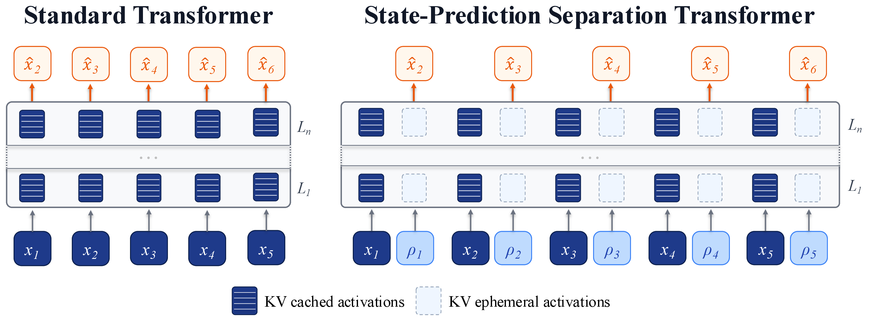

Figure 1: Standard versus State-Prediction Separation Transformer. Top: The standard Transformer uses the same hidden states for both memory and prediction. Our variant separates these roles: input token \(x_i\) time steps form a persistent state, while prediction token steps \(\rho_i\) produce next-token predictions. Bottom: At 1.6B parameters, State-Prediction Separation matches the validation loss of a standard Transformer trained on \(47\)B tokens while using \(2.6\times\) fewer tokens (pre-decay). At an \(18\)B-token pre-decay budget, it already achieves \(\Delta\mathrm{NLL}=-0.071\) versus standard..
1 Introduction↩︎
Attention-based architectures, including the Transformer [1] and earlier recurrent designs [2], have dual use for the activations computed at each time step: they are used to predict the output of that time step (i.e., token in language models) and are attended to by subsequent steps. The first role is focused on prediction; the second on capturing state information to be reused later on. Generally, these two functions are entangled in the same representation and computation stream (i.e., forward path). In this paper, we propose and study the following hypothesis in large language models (LLMs):
Hypothesis: State-Prediction Separation (SPS; informal)
The next-token prediction computation and state representation compete when forced through the same computation. Routing them through separate streams yields better language modeling.
Technically, we separate the state and prediction functionalities by inserting an additional computation time step before predicting the next token (1). Time steps then appear in pairs: first, the token previously generated is processed, but no new token is emitted. An additional time step follows, which emits the next token to generate. The key-value (KV) entries from the first of the two steps are added to the KV cache, while the entries of the latter of the two are discarded.1 This design distinguishes between two streams: a state stream and a prediction stream.
We conduct extensive experiments pretraining a set of LLMs at common research scales, from 53M to 1.678B parameters. The main result is that SPS significantly improves pretraining performance over standard Transformers in both token-equivalent and compute-equivalent settings. 1 illustrates one of the key results: non-separating baselines cannot match the training loss of an SPS Transformer even with double the number of training tokens. We also show that state-prediction separation outperforms several variants controlling for SPS’s compute and memory overheads, proving that separation is the key component in the improvements we report.
Our code is available at https://github.com/lil-lab/sps.
2 Prediction and State Preparation↩︎
We consider a standard autoregressive Transformer with vocabulary \(V\), depth \(L\), and parameters \(\theta\). 8 details the full architecture. The input is a sequence \(x = (x_1,\ldots,x_T)\). At sequence position \(i\) with input token \(x_i\), the model computes a per-layer hidden state \(h_i^{(l)} \in \mathbb{R}^d\), where \(l=1,\dots,L\), \(h_i^{(0)}\) is the token embedding, and \(h_i^{(L)}\) the final representation. Each position \(i\) also contributes entries to the key-value (KV) cache. Through causal attention, all the past keys and values (i.e., from positions \(k < i\)) contribute to the final representation \(h_i^{(L)}\), which is then used to compute the next-token distribution. Each hidden state \(h_i^{(l)}\) plays two roles: it is part of the computation of the immediate prediction for \(x_{i+1}\), and it produces KV entries read by every later position.
This double role is reflected in the optimization gradients, as they are computed through backpropagation. The language modeling training loss is \(\mathcal{L} = \frac{1}{T-1}\sum_{i=1}^{T-1} \ell_i\), with the per-position cross-entropy loss \(\ell_i = -\log p(x_{i+1}\mid x_{\le i})\). The parameters \(\theta\) are used repeatedly in each position \(i=1,\dots,T\) in the Transformer. We isolate the gradients for each position \(i\) by denoting \(\nabla_{\theta_i}\mathcal{L}\), and can similarly denote \(\nabla_{\theta_i}\ell_j\) to denote the gradients for position \(i\) from the loss at position \(j\).2 The gradients of the loss \(\mathcal{L}\) by \(\theta\) are the linear sum of all per-position gradients: \[\nabla_\theta\mathcal{L} \;=\; \sum_{i=1}^{T-1} \nabla_{\theta_i}\mathcal{L} \;=\; \frac{1}{T-1}\sum_{i=1}^{T-1}\sum_{j=1}^{T-1}\nabla_{\theta_i}\ell_j \;=\; \frac{1}{T-1}\sum_{i=1}^{T-1}\sum_{j=i}^{T-1}\nabla_{\theta_i}\ell_j \;\;.\label{eq:causal-grad}\tag{1}\] The last term follows pruning every non-causal \(\ell_j\), because of the causality in attention, each step’s parameters affect only the current and future losses. Separating the step’s own loss (\(j=i\)) from the losses back-propagated only through the KV cache (\(j>i\)) decomposes the gradient by source: \[\label{eq:aggregate-grad} \nabla_{\theta}\mathcal{L} \;=\; \sum_{i=1}^{T-1}\;[\; \underbrace{\vphantom{\sum_{i=j+1}^{T-1}}\tfrac{1}{T-1}\nabla_{\theta_i}\ell_i}_{\text{Prediction}} \;+\; \underbrace{\tfrac{1}{T-1}\sum_{j=i+1}^{T-1} \nabla_{\theta_i}\ell_j }_{\text{State}}\;]\;\;.\tag{2}\]
Time step \(i\) contributes gradients for the prediction of \(x_{i+1}\) — the prediction task — and for the preparation of keys and values that help all later positions \(j>i\) make better predictions — the state representation task. Both components flow (i.e., back-propagate) through the same hidden state \(h_i^{(l)}\), which is therefore optimized to conflate the two roles in a single set of activations.
3 The State-Prediction Separation Transformer↩︎
We separate the two roles by augmenting the standard Transformer with an additional learned token, <predict>, inserted after every input token. Given an input sequence \(x=(x_1,\ldots,x_T)\), we form
an augmented sequence by interleaving dummy tokens \(\rho_i\), all set to a new <predict> token: \[\label{eq:interleaved} x
\rightarrow (x_1,\rho_1,\; x_2,\rho_2,\; \ldots,\; x_T,\rho_T)\;\;.\tag{3}\] The two tokens \(x_i\) and \(\rho_i\) at index \(i\) share the
same position encoding. The model now maintains two interleaved streams of representations: an input stream \(\{x_i\}_{i=1}^T\) that we use to carry the state forward, and a prediction stream \(\{\rho_i\}_{i=1}^T\) that we use to emit next-token predictions. Beyond a sliding window of size \(w\), only key-value elements from the input stream positions are available in the KV cache, to
be attended by later positions. The sliding window allows to attend to the specific token-choice representations for a short horizon (i.e., for local coherence). The prediction \(x_{i+1}\) is done at the position of \(\rho_i\), so the loss is applied only at \(\rho_i\) positions: \[\label{eq:sps-loss} \mathcal{L} =
\frac{1}{T-1}\sum_{i=1}^{T-1} -\log p\bigl(x_{i+1} \mid x_1,\rho_1,\ldots,x_i,\rho_i\bigr)\;\;.\tag{4}\]
In a standard Transformer, the two streams are tied together: \(\rho_i\) does not exist, and the same representations \(h_i^{(l)}\) at each position must simultaneously pack the information to emit the prediction for \(x_{i+1}\) and produce the keys and values read by every later position. The two gradient components of 2 (the prediction term \(\nabla_{\theta_i}\ell_i\) and the state-preparation term \(\sum_{j>i}\nabla_{\theta_i}\ell_j\)) are routed through one and the same \(h_i^{(\ell)}\), with no architectural separation. 1 illustrates the State-Prediction Separation Transformer (SPS), and compares it to the standard architecture.
We can now make the informal hypothesis from 1 precise in this two-stream notation:
Hypothesis: State-Prediction Separation (formal)
The prediction gradients \(\nabla_{\theta_{\rho_i}}\ell_i\) and the state-preparation gradients \(\sum_{j>i}\nabla_{\theta_{x_i}}\ell_j\) are both used to optimize the computation of the same representations \(h_i\), thereby competing with each other in the standard Transformer. Separating the hidden representations to \(h_{\rho_i}\) and \(h_{x_i}\) and routing the gradients appropriately separates the two functions, and yields lower next-token loss at matched parameter count.
At training time, we realize this separation through an attention mask. In SPS, input entries are persistent, while <predict> entries are evicted once they leave a sliding window of size \(w\). A query \(q\) at step \(i\) (i.e., either \(x_i\) or \(\rho_i\)) attends to all causal
input entries and only recent <predict> entries. The only difference between input and prediction positions is that prediction positions attend to their corresponding input position: \[\label{eq:sps-mask} \mathcal{A}_{\mathrm{SPS}}(i,q) = \underbrace{\{x_k : k \leq i\}}_{\text{All causal inputs}} \;\cup\; \underbrace{ \begin{cases} \{\rho_k : i-w \leq k < i\} & \text{if } q=x_i\\ \{\rho_k : i-w \leq k \leq
i\} & \text{if } q=\rho_i \end{cases}}_{\text{Recent \texttt{<predict>} entries}}\;\;.\tag{5}\] The persistent KV cache of SPS contains only input entries; <predict> entries are read
by at most \(w\) later queries before being discarded. This routes the two gradient components of 2 to different streams. Input representations \(h_{x_i}^{(l)}\) are visible to every later query, so they accumulate the full state-preparation gradient \(\sum_{j>i}\nabla_{h_{x_i}^{(l)}}\ell_j\). <predict>
representations \(h_{\rho_i}^{(l)}\) are visible only within a window. Their gradient is dominated by the immediate prediction term \(\nabla_{\theta_{\rho_i}}\ell_i\), with a contribution
limited to at most \(w-1\) following state-preparation losses. 1 contrasts a standard Transformer with our SPS Transformer.
3.0.0.1 Training Efficiency
Our method increases compute in order to separate the state and prediction streams, which makes training more expensive due to the doubled context length. We efficiently simulate the sliding window through attention masking, and apply the same mechanism to prevent attention from crossing document boundaries.
3.0.0.2 Inference Efficiency
The additional cost is negligible at inference. Forwarding one or a few tokens simultaneously incurs essentially the same latency. This is a well-known property that motivates speculative decoding [3], [4]. Concretely, SPS’s persistent KV cache contains only input tokens, matching the size of a standard Transformer cache, with a bounded \(w\)-slot ring buffer
holding the most recent <predict> entries. Each generated token triggers a single decode step that forwards the pair \((x_i, \rho_i)\) jointly and reads next-token logits from the
<predict> hidden state.
4 Experimental Setup↩︎
4.0.0.1 Baselines
We compare SPSto a standard Transformer (Standard) and to two ablations. The first, 2x Memory, retains both input and <predict> entries in
the KV cache throughout the sequence. The model gains computational capacity from its doubled context length, but its persistent memory footprint also doubles, and <predict> entries still serve both prediction and state-preparation.
The second, Delayed State, inserts a <predict> token after every input, giving the model an extra computation step before each prediction, but commits the persistent state at the
<predict> slot, one step after the input. Compared to SPS, this variant delays state preparation as well, and performs both prediction and state preparation together at the
<predict> slot. A query \(q\) at step \(i\) attends to the \(w\) most recent input entries, using the same fixed-size ephemeral window as
SPSbut populated by input entries rather than <predict> entries, and to all causal <predict> entries.
Delayed Statekeeps the persistent KV cache size roughly equivalent to Standard’s. However, unlike SPS, no separation between roles is enforced. The
<predict> stream carries both prediction and state. Delayed Statetherefore differs from SPSonly in whether the two streams are separated.
| XS | S | M | L | XL | |
|---|---|---|---|---|---|
| Layers (\(L\)) | 8 | 12 | 24 | 36 | 48 |
| Hidden size (\(d\)) | 512 | 768 | 1024 | 1280 | 1600 |
| Heads (\(H\)) | 8 | 12 | 16 | 20 | 25 |
| FFN size | 1536 | 2304 | 3072 | 3840 | 4800 |
| Parameters | 53M | 131M | 379M | 831M | 1.678B |
r0.55 4pt
All variants share the same backbone, a pre-normalized Transformer blocks with RMSNorm [5], SwiGLU feed-forward networks [6] of intermediate size \(3d\), rotary positional embeddings [7], no biases on linear layers, a weight-tied unembedding, and a context length of \(4{,}096\) tokens. We evaluate five scales, summarized in 1. For S, M, L, and XL, we follow the GPT-2 [8] recipe, and we add XS as a smaller scale. SPS, 2x Memory, Delayed State, and Reverse SPSuse the same backbone, parameter count, and hyperparameters as Standardat every scale, differing only in attention pattern. Unless otherwise specified, all sliding-window variants use \(w{=}64\) at every scale.
4.0.0.2 Data
We pretrain on FineWeb-Edu [9], a high-quality educational subset of FineWeb, and tokenize with the GPT-2 tokenizer. Sequences are packed
across document boundaries, with an end-of-sequence token (<eos>) inserted between consecutive documents to delimit them. Attention is masked so that queries within a document cannot attend to keys from any other document, and we exclude
<eos> positions from the next-token loss so that the model is never trained to predict the start of an unrelated document. Each model is trained for \(20\)B tokens by default. This budget meets or exceeds
the Chinchilla compute-optimal ratio of \({\approx}20\) tokens per parameter [10] at every scale, except for
XL (which is under-trained due to its higher cost of training).3 To obtain a fair GPU-hours comparison, we additionally train Standard for
\(40\)B tokens (except for XL, that is trained for 47B tokens, until it matches SPS validation loss). All runs see the same data in the same order.
4.0.0.3 Training
We base our training code on nanoGPT [11], including its standard hyperparameters.4 The global batch size is \(96\) sequences of length \(4{,}096\), i.e.,\(\approx\!400{,}000\) tokens per gradient update.
All models are trained in bfloat16 mixed precision. We use a learning-rate schedule [12] consisting of a brief linear warmup, a constant
phase at the peak learning rate, and a linear decay covering the final \(10\%\) of training tokens. For faster training, we adapt the open-source Triton implementation of FlashAttention [13] to support the sliding-window and <predict>-token attention patterns of SPS, Delayed State, and 2x Memory, so that all variants train at comparable throughput; we found alternatives such as FlexAttention [14] to be either memory-inefficient or substantially slower in our setting. All XS/S/M/L runs use \(2\) NVIDIA H100 \(80\) GB GPUs, while all XL runs use \(2\) NVIDIA B200 GPUs, with data-parallel distributed training. All runs in the main results use a single
seed (i.e., the data ordering and weight-initialization seed are matched across methods).
4.0.0.4 Evaluation
We report three families of metrics. (a) Validation loss. Held-out NLL on FineWeb-Edu, our pretraining distribution. (b) Generalization. Corpus NLL averaged over four out-of-distribution corpora (WikiText [15], C4 [16], Pile-Books3 [17], GovReport [18]), and zero-shot accuracy averaged over five standard benchmarks (ARC-Easy [19], HellaSwag [20], PIQA [21], SciQ [22], LAMBADA [23]), evaluated as standard practice via the LM Evaluation Harness [24]. (c) Inference efficiency. End-to-end throughput (tokens/s) and peak GPU memory measured on a single NVIDIA H100 for a batch of \(16\) sequences with a prefill of \(1024\) tokens followed by \(3072\) decode steps, reported as ratios relative to Standard at the same scale. Every method runs through the same generation loop, KV-cache layout, and Triton attention path, with each method using the fused kernel matched to its own attention pattern.
5 Results↩︎

| Validation Loss | Generalization | Inference Efficiency | ||||||||||||||||||||||||||||||||||||||||||||||||||||||||||||||||||||||||||||||||||||||||||||||
|---|---|---|---|---|---|---|---|---|---|---|---|---|---|---|---|---|---|---|---|---|---|---|---|---|---|---|---|---|---|---|---|---|---|---|---|---|---|---|---|---|---|---|---|---|---|---|---|---|---|---|---|---|---|---|---|---|---|---|---|---|---|---|---|---|---|---|---|---|---|---|---|---|---|---|---|---|---|---|---|---|---|---|---|---|---|---|---|---|---|---|---|---|---|---|---|---|
| 3-3 (lr)4-5 (lr)6-7 Size | Method | FineWeb-Edu (\(\downarrow\)) | Corpus NLL (\(\downarrow\)) | Task Accuracy (%, \(\uparrow\)) | Throughput (\(\times\), \(\uparrow\)) | Peak Memory (\(\times\), \(\downarrow\)) | ||||||||||||||||||||||||||||||||||||||||||||||||||||||||||||||||||||||||||||||||||||||||||
| XS | 3.107 | 4.335 | 44.9 | 1.00 | 1.00 | |||||||||||||||||||||||||||||||||||||||||||||||||||||||||||||||||||||||||||||||||||||||||||
| 3.073 (\(-0.034\)) | 4.311 (\(-0.024\)) | 47.3 (\(+2.4\)) | 0.93 (\(-0.07\)) | 1.81 (\(+81\%\)) | ||||||||||||||||||||||||||||||||||||||||||||||||||||||||||||||||||||||||||||||||||||||||||||
| 3.086 (\(-0.021\)) | 4.312 (\(-0.023\)) | 46.9 (\(+2.0\)) | 0.94 (\(-0.06\)) | 1.01 (\(+1\%\)) | ||||||||||||||||||||||||||||||||||||||||||||||||||||||||||||||||||||||||||||||||||||||||||||
| 3.065 (\(-0.042\)) | 4.243 (\(-0.092\)) | 47.3 (\(+2.5\)) | 0.94 (\(-0.06\)) | 1.01 (\(+1\%\)) | ||||||||||||||||||||||||||||||||||||||||||||||||||||||||||||||||||||||||||||||||||||||||||||
| (l2ptr2pt)1-7 | 2.858 | 4.018 | 49.5 | 1.00 | 1.00 | |||||||||||||||||||||||||||||||||||||||||||||||||||||||||||||||||||||||||||||||||||||||||||
| 2.829 (\(-0.030\)) | 3.981 (\(-0.036\)) | 51.1 (\(+1.5\)) | 0.93 (\(-0.07\)) | 1.81 (\(+81\%\)) | ||||||||||||||||||||||||||||||||||||||||||||||||||||||||||||||||||||||||||||||||||||||||||||
| 2.829 (\(-0.029\)) | 3.992 (\(-0.026\)) | 51.8 (\(+2.2\)) | 0.94 (\(-0.06\)) | 1.01 (\(+1\%\)) | ||||||||||||||||||||||||||||||||||||||||||||||||||||||||||||||||||||||||||||||||||||||||||||
| 2.810 (\(-0.048\)) | 3.913 (\(-0.105\)) | 51.8 (\(+2.3\)) | 0.94 (\(-0.06\)) | 1.01 (\(+1\%\)) | ||||||||||||||||||||||||||||||||||||||||||||||||||||||||||||||||||||||||||||||||||||||||||||
| (l2ptr2pt)1-7 | 2.648 | 3.732 | 55.8 | 1.00 | 1.00 | |||||||||||||||||||||||||||||||||||||||||||||||||||||||||||||||||||||||||||||||||||||||||||
| 2.610 (\(-0.038\)) | 3.687 (\(-0.045\)) | 57.3 (\(+1.4\)) | 0.93 (\(-0.07\)) | 1.81 (\(+81\%\)) | ||||||||||||||||||||||||||||||||||||||||||||||||||||||||||||||||||||||||||||||||||||||||||||
| 2.611 (\(-0.037\)) | 3.701 (\(-0.031\)) | 57.5 (\(+1.7\)) | 0.95 (\(-0.05\)) | 1.01 (\(+1\%\)) | ||||||||||||||||||||||||||||||||||||||||||||||||||||||||||||||||||||||||||||||||||||||||||||
| 2.591 (\(-0.058\)) | 3.627 (\(-0.106\)) | 58.7 (\(+2.9\)) | 0.95 (\(-0.05\)) | 1.01 (\(+1\%\)) | ||||||||||||||||||||||||||||||||||||||||||||||||||||||||||||||||||||||||||||||||||||||||||||
| (l2ptr2pt)1-7 | 2.537 | 3.598 | 60.1 | 1.00 | 1.00 | |||||||||||||||||||||||||||||||||||||||||||||||||||||||||||||||||||||||||||||||||||||||||||
| 2.495 (\(-0.042\)) | 3.542 (\(-0.055\)) | 62.1 (\(+1.9\)) | 0.83 (\(-0.17\)) | 1.78 (\(+78\%\)) | ||||||||||||||||||||||||||||||||||||||||||||||||||||||||||||||||||||||||||||||||||||||||||||
| 2.491 (\(-0.045\)) | 3.532 (\(-0.066\)) | 61.3 (\(+1.2\)) | 0.90 (\(-0.10\)) | 1.01 (\(+1\%\)) | ||||||||||||||||||||||||||||||||||||||||||||||||||||||||||||||||||||||||||||||||||||||||||||
| 2.470 (\(-0.067\)) | 3.484 (\(-0.113\)) | 62.6 (\(+2.5\)) | 0.90 (\(-0.10\)) | 1.01 (\(+1\%\)) | ||||||||||||||||||||||||||||||||||||||||||||||||||||||||||||||||||||||||||||||||||||||||||||
| (l2ptr2pt)1-7 | 2.458 | 3.487 | 63.2 | 1.00 | 1.00 | |||||||||||||||||||||||||||||||||||||||||||||||||||||||||||||||||||||||||||||||||||||||||||
| 2.411 (\(-0.047\)) | 3.423 (\(-0.064\)) | 64.3 (\(+1.0\)) | 0.64 (\(-0.36\)) | 1.75 (\(+75\%\)) | ||||||||||||||||||||||||||||||||||||||||||||||||||||||||||||||||||||||||||||||||||||||||||||
| 2.410 (\(-0.048\)) | 3.433 (\(-0.055\)) | 64.8 (\(+1.6\)) | 0.94 (\(-0.06\)) | 1.01 (\(+1\%\)) | ||||||||||||||||||||||||||||||||||||||||||||||||||||||||||||||||||||||||||||||||||||||||||||
| 2.390 (\(-0.068\)) | 3.338 (\(-0.149\)) | 66.3 (\(+3.1\)) | 0.94 (\(-0.06\)) | 1.01 (\(+1\%\)) | ||||||||||||||||||||||||||||||||||||||||||||||||||||||||||||||||||||||||||||||||||||||||||||
6pt
5.0.0.1 Performance and Efficiency
2 summarizes performance and efficiency findings. SPSattains the lowest validation NLL on FineWeb-Edu at every scale, with the gap over Standardwidening from \(-0.042\) at XS to \(-0.068\) at XL. 2 shows that at matched training tokens SPSreaches lower validation NLL than Standardthroughout training (top), and that at matched GPU-hours SPSeventually overtakes Standardat every scale (bottom). Even doubling Standard’s pre-decay training budget from \(18\)B to \(36\)B tokens does not close the gap. SPSthus reaches Standard’s quality on roughly half the training data, with the data-efficiency ratio widening as scale grows. This is an important property as high-quality human-generated text approaches projected exhaustion [25]. The improvement carries over to held-out generalization. Corpus NLL on four out-of-distribution corpora drops by \(0.09\)–\(0.11\) across scales, and zero-shot accuracy on five standard benchmarks improves by \(2.3\)–\(3.1\%\). 3 shows this trend directly. Crucially, this quality gain comes at minimal increase in inference cost. SPS’s persistent KV cache is the same size as Standard’s (peak memory ratio \(1.01\)), and end-to-end throughput is within \(6\)–\(10\%\) of Standardat all scales. While each result above is from a single training run, we verify with a \(3\)-seed sweep at S, \(10\)B that SPS’s gap over Standard, Delayed State, and 2x Memoryis significant at \(p<0.005\) (one-sided Welch’s \(t\)-test; 10).
Takeaway :SPSoutperforms Standardin validation loss, generalization, and learning speed at every scale, matching Standard’s persistent memory footprint and inference throughput while reaching Standard’s quality on roughly half the training data.
5.0.0.2 State and Prediction Role Separation
2x Memorykeeps every <predict> entry persistent at the same per-step compute as SPS, which discards <predict> entries beyond the window. SPSis consistently better in validation NLL across XS–XL, even though it has half the persistent KV cache. This shows that the gain is not capacity-based. Keeping <predict> entries persistent forces each one to
serve both as a prediction site and as a state carrier for later queries, re-coupling the two streams that SPSseparates.
A second hypothesis is that SPSbenefits only from giving the model an additional Transformer step before the persistent state is committed. Delayed Statetests this directly. It has the same
per-step compute as SPSand the same persistent-cache size as Standardand SPS, but commits the persistent state at the <predict> slot, one step
after the input, and so does not separate the two roles. Delayed Statedoes improve over Standard, confirming that the extra computation step carries some benefit, but at every scale
SPSremains consistently better, by \(0.019\)–\(0.021\) in validation NLL and by \(0.06\)–\(0.07\) in corpus NLL (2).
Takeaway :The specific structure of state-prediction separation in SPS matters more than extra computations or even simply doubling the memory.
5.0.0.3 Which Stream Should Persist, and at What Window?
We additionally run a Reverse SPS variant that swaps the two roles. <predict> entries from the persistent state and input entries are windowed and used to emit the next-token prediction. This is the
mirror image of SPS, which predicts from <predict> and stores state from input. This isolates whether the specific role assignment matters. We jointly ablate the <predict>-window size
\(w\) and the choice of persistent stream at the S scale, where a sweep is cheap to run, and reuse the resulting \(w\) across all scales in the main experiments ([fig:window95ablation]). Both SPSand Delayed Stateshow nearly constant performance across all
\(w \in \{0, 16, 64, 256\}\), with \(w{=}64\) as the empirical best by a small margin; we therefore fix \(w{=}64\) at every scale. Reverse SPS matches SPSat moderate \(w\) but degrades sharply at small \(w\), where windowing the input stream cuts off recent input
visibility. SPS’s ordering is the more robust default: persisting inputs tolerate a wider range of \(w\) before quality drops.
Takeaway :SPSis robust to window size, while Reverse SPScollapses at small \(w\). Persisting the input stream is the more forgiving design.
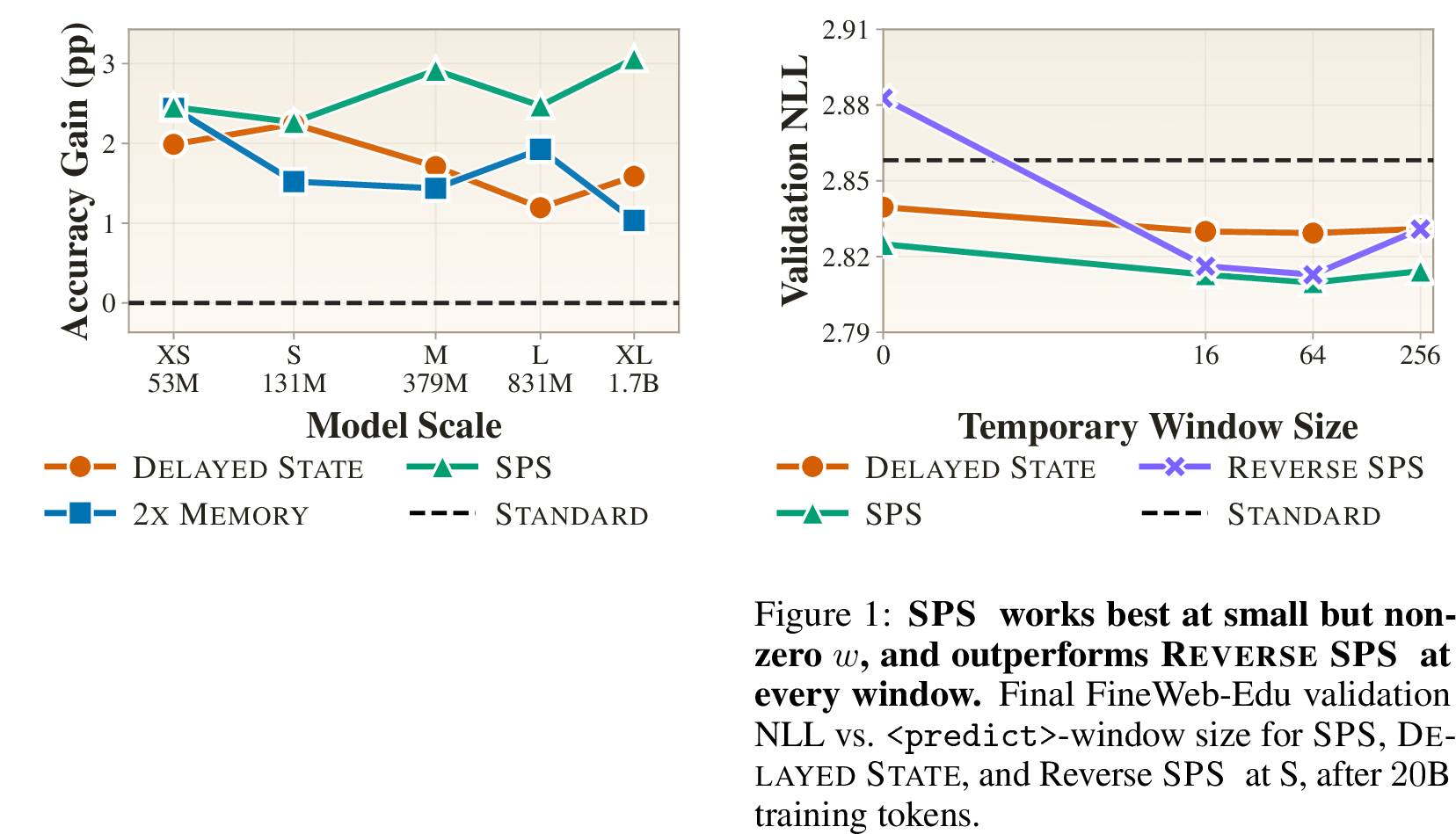


Figure 4: Analysis of SPS. (a) Where future-loss gradient lands during training. (b) How much the persistent state is actually used at inference.. a — Per-offset gradient ratio \(r(p,\,k)\) for Standard, SPS, and Delayed State. For SPS and Delayed State, solid curves are the input stream (\(p{=}x_i\)) and dotted curves the prediction stream (\(p{=}\rho_i\)). Bold curves are Savitzky–Golay–smothed [26] trends. The faint curves underneath are the raw per-offset means. SPS’s input stream consistently sustains more future-loss gradient; Delayed State’s prediction stream stays low, and its input stream collapses past the ephemeral window \(k{=}64\)., b — Per-position NLL degradation when each method’s persistent state is restricted to a window of size \(w{=}64\), plotted against the document-relative query position \(t\) at each scale. Bold curves are Savitzky–Golay–smoothed [26] trends. The faint curves underneath are the raw per query position means. SPS’s curve sits uniformly above Delayed State’s, with the late-position gap ranging from \(\sim\!2.0\times\) at XS to \(\sim\!1.3\times\) at XL. SPS’s persistent keys carry more future-relevant information and evicting them is more hurtful.
5.0.0.4 Analysis: Why Does Separation Help?
Following 2 , we probe how each architecture allocates gradients between the prediction role (the immediate loss \(\ell_i\)) and the state representation role (future losses \(\ell_j\), \(j > i\)) at training time, and what this implies at inference. Recall that we denote as \(\nabla_i \ell_j\) the gradients from the loss term \(\ell_j\) due to the use of the parameters in position \(i\).
In SPSand Delayed Stateeach step \(i\) occupies two positions in the interleaved sequence: an input slot \(x_i\) where the input token is read, and a predict slot \(\rho_i\) where the cross-entropy \(\ell_i\) is computed (the only position where a prediction happens). Both positions use the parameters \(\theta\). Therefore, we can separate the gradients to \(\nabla_{x_i}\ell_j\) and \(\nabla_{\rho_i}\ell_j\). Because \(x_i\)’s hidden states feed into \(\rho_i\), both slots receive non-zero gradient from \(\ell_i\) even though the loss is realized only at \(\rho_i\). This is in contrast to Standard, where each step occupies a single position with gradients \(\nabla_i \ell _j\).
For every source position \(p\) at step \(i\) (so \(p \in \{x_i, \rho_i\}\) in SPSand Delayed
State, \(p = x_i\) in Standard), we isolate \(\nabla_p \ell_{i+k}\), the gradients from the step-\(k\)-ahead loss, and
compute the ratio5 \[r(p,\,k) \;=\; \frac{\bigl\lVert \nabla_{\theta_p}\, \ell_{i+k} \bigr\rVert_2}{\bigl\lVert \nabla_{\theta_p}\, \ell_i
\bigr\rVert_2}\;\;,\] the magnitude of position-\(p\) gradients coming from the loss \(k\) steps ahead relative to the current time step gradients. We average \(r\) over \(8{,}000\) examples (\(1{,}000\) documents, \(8\) source positions each) for \(k \le
512\), separately on input positions (\(p{=}x_i\)) and prediction positions (\(p{=}\rho_i\)) for SPS and Delayed State.
4 (a) shows a clean dichotomy. SPS’s input stream carries more future-loss gradient than Standard at every offset, and its prediction stream carries
strictly less, meaning the two roles are routed to different tokens. Delayed State reduces this separation. Its prediction stream stays uniformly low, and its input stream falls below SPS past
the <predict> window \(k{=}64\), beyond which gradient can only flow indirectly. A single stream does not allow the model to effectively learn to predict and to represent state.
Carrying future-loss gradient is necessary but not sufficient, the persistent state must also be important at inference. We test this by restricting each variant’s persistent state to a sliding window of size \(\omega\) (distinct from the prediction window \(w\)) and measuring the resulting NLL degradation. For a trained model \(M \in \{\mathrm{\small SPS},\,\mathrm{\small Delayed State}\}\), we define \(M_\omega\) as \(M\) used with a forced sliding persistent-cache of size \(\omega\), \(\ell_i(M)\) as the loss of the vanilla model \(M\) at position \(i\), and \(\ell_i(M_\omega)\) is the loss of the altered \(M_\omega\) at the same position \(i\). We measure \[\Delta\ell_i(M_\omega) \;=\; \ell_i(M_\omega) - \ell_i(M),\] for document positions \(i \in \{1,\dots,2048\}\). We set a small \(\omega=64\) (as opposed to the vanilla \(4{,}096\)) and average each \(\Delta\ell_i\) across \(8{,}000\) documents. A larger \(\Delta\ell_i\) means more of \(M\)’s long-range prediction depends on persistent keys outside the \(\omega\)-window. 4 (b) shows that ablating SPS’s out-of-window persistent state hurts NLL \(1.4\)–\(2.2\times\) more than ablating Delayed State’s across scales, although with the full persistent cache SPS performs better than Delayed State. Therefore, the future-loss gradient SPS routes onto the input stream actually translates into a persistent state the model relies on at inference.
Takeaway :SPS better separates present-loss and future-loss gradients and produces a persistent state more important at inference compared to Delayed State.
6 Related Work↩︎
6.0.0.1 Tension Between Present and Future Predictions
Each hidden state in a Transformer is asked to do two jobs at once: encode the next-token prediction at its own position, and prepare the persistent state that later positions will read from. [27] study this tension precisely by contrasting two hypotheses: breadcrumbs (the keys and values useful for the current prediction also serve future ones) and pre-caching (some
computation in early positions is targeted at later predictions and would be wasted on the current one). They find pre-caching in pretrained Pythia, increasing with scale, consistent with mechanistic evidence that earlier-position representations already
encode upcoming-token information [28], [29]. The early two-stream
attention of XLNet [30] also distinguishes prediction from content, but in service of permutation language modeling rather
than to relieve pre-caching under standard left-to-right training. SPSis a direct architectural response to this tension. Rather than asking one stream to serve both jobs, it inserts a dedicated <predict>
slot at every position to carry the next-token prediction, freeing the input stream to specialize as persistent state. If the two-jobs view is right, separating the roles should help. Our experiments confirm this at every scale.
6.0.0.2 Adding Compute on the Input Side
One approach to relieve this tension is adding computation at input positions. [31] append <pause> tokens to the prompt
so the model gets extra forward passes before answering, motivated by the fact that Transformer expressivity is bounded by context length [32].
[33] use the same insertion as filler tokens during training. These methods share SPS’s mechanism of adding extra
tokens, but use it to add capacity rather than to separate the two roles. Our Delayed Stateand 2x Memorybaselines isolate this distinction. Both retain the inserted-token mechanism and the extra
compute, but do not enable the separation, and both underperform SPSat every scale.
6.0.0.3 Enriching the Future-Prediction Signal
A complementary line of work intervenes on the prediction target. [34] show that teacher-forced next-token prediction can
silently fail on planning tasks where one step is hard and the rest are easy, motivating training signals that reach beyond the immediate next token. Multi-token-prediction methods [35]–[40] and belief-state objectives [41], [42] address this by adding auxiliary losses at non-current positions to strengthen the future-prediction signal itself. SPSpursues a different goal. We do not
enrich what is predicted, but separate where prediction and state-preparation take place. By routing the next-token loss onto a dedicated <predict> slot, SPSrelieves the present-future tension structurally,
while remaining compatible with these approaches.
7 Discussion↩︎
We introduce the SPS hypothesis that posits that the two tasks each hidden state must perform, predicting the next token and preparing state for later predictions, interfere when forced through one representation, and that separating them structurally should help. We study the hypothesis with the SPS Transformer, which realizes this separation via two interleaved streams, using non-persistent states for prediction. The experiments are decisive: at every scale from XS to XL, SPSlowers FineWeb-Edu validation NLL, improves held-out-corpus NLL, and raises zero-shot accuracy, at the same persistent KV-cache footprint as the standard Transformer and within a few percent of its throughput. Our experiments show that separation is key to the observed improvement. Our gradient-flow and restricted-state analyses confirm the mechanism: SPSroutes future-loss gradient onto the input stream and produces a persistent state significantly more impactful for future states than alternatives. SPSshows dramatic data efficiency gains, which increase monotonically across XS–XL, suggesting it would only grow with more compute. This matters in a regime where high-quality data is finite and approaching projected exhaustion [25]. Learning more from each token directly extends the runway for pretraining.
Compute constrains the scope of our evidence in two ways. First, we pretrain on a single corpus (FineWeb-Edu); the consistent gains on out-of-distribution corpora and zero-shot benchmarks suggest the trends transfer beyond it, but we could not tested alternative pretraining mixtures. Second, our largest scale is \(1.678\)B parameters; the SPS-vs-StandardNLL gap monotonically widens across XS–XL, suggesting the trend should continue past 1.6B, but this requires further verification. Our argument that mixing prediction and state-preparation in one hidden state is suboptimal rests on controlled ablations and gradient/state analyses; a formal characterization of when and how much this conflation hurts, as a function of capacity, depth, or data, would tighten the case and is left for future work. SPS’s prediction stream adds a forward-pass slot per input position, roughly doubling per-step training compute over the standard Transformer; whether the same separation can be obtained at lower overhead, via shallower or narrower computation on the prediction stream, or a sparser persistent state, is an open and practically valuable question. The two streams currently also share all parameters. We leave for future work whether further separating them (e.g., via distinct attention/FFN parameters per stream) could yield further gains now that the roles are decoupled.
Acknowledgments↩︎
This research was partially supported by a gift to the LinkedIn–Cornell Bowers Strategic Partnership; AI-MI and NSF Award 2433348; the National Science Foundation NSF under award OAC-2311521; and NASA under award No. 20-OSTFL20-0053. NG is supported by an Empire AI Postdoctoral Fellowship. Any opinions, findings and conclusions or recommendations expressed in this material are those of the author(s) and do not necessarily reflect the views of the National Science Foundation or of NASA. We thank the members of the Cornell LIL Lab for helpful discussions. KB acknowledges this work has been made possible in part by a gift from the Chan Zuckerberg Initiative Foundation to establish the Kempner Institute for the Study of Natural and Artificial Intelligence.
8 Full Transformer Notation↩︎
Let \(V\) denote a finite vocabulary. An autoregressive Transformer defines a distribution \(p \colon V^{\leq T} \to \Delta(V)\) mapping a sequence of tokens to a distribution over the next token.
The model consists of \(L\) Transformer layers, with \(H\) attention heads each, with dimensions \(d_h = d/H\). For any given sequence position \(i\), each token \(x_i\) is mapped to an embedding \(h_i^{(0)} = E_{x_i} \in \mathbb{R}^d\), where \(E \in \mathbb{R}^{|V| \times d}\) is a learned embedding matrix (so \(E_{x_i}\) denotes its \(x_i\)-th row).
The embeddings are processed by \(L\) blocks combining causal multi-head self-attention (\(\mathrm{MHA}\)) with a position-wise feed-forward network (\(\mathrm{FFN}\)) and normalization layers (\(\mathrm{Norm}\)), producing the per-layer hidden states \(h_i^{(l)} \in \mathbb{R}^d\). For \(l = 1, \ldots, L\):\[\begin{align} \tilde{h}_i^{(l)} &= h_i^{(l-1)} + \mathrm{MHA}^{(l)}\!\bigl( \mathrm{Norm}^{(l)}_{\mathrm{MHA}}(h^{(l-1)})\bigr)_i,\\ h_i^{(l)} &= \tilde{h}_i^{(l)} + \mathrm{FFN}^{(l)}\!\bigl( \mathrm{Norm}^{(l)}_{\mathrm{FFN}}(\tilde{h}_i^{(l)})\bigr). \end{align}\] Let \(\bar{h}_i^{(l)} \mathrel{\vcenter{:}}= \mathrm{Norm}^{(l)}_{\mathrm{MHA}}(h_i^{(l-1)})\) denote the normalized input to layer \(l\). Each head \(\eta \in \{1, \ldots, H\}\) is parameterized by projection matrices \(W_Q^{(l,\eta)}, W_K^{(l,\eta)}, W_V^{(l,\eta)} \in \mathbb{R}^{d_h \times d}\) and computes \[\label{eq:qkv} q_i^{(l,\eta)} = W_Q^{(l,\eta)} \bar{h}_i^{(l)}, \qquad k_i^{(l,\eta)} = W_K^{(l,\eta)} \bar{h}_i^{(l)}, \qquad v_i^{(l,\eta)} = W_V^{(l,\eta)} \bar{h}_i^{(l)}.\tag{6}\] A rotary positional transform \(\mathcal{R}_i\) is applied to queries and keys, and the per-head output is obtained by causally masked attention, then concatenated across heads and mixed by an output projection \(W_O^{(l)} \in \mathbb{R}^{d \times d}\): \[\begin{align} o_i^{(l,\eta)} &= \sum_{j \leq i} \mathrm{softmax}_{j}\!\left( \frac{(\mathcal{R}_i q_i^{(l,\eta)})^{\!\top} (\mathcal{R}_j k_j^{(l,\eta)})}{\sqrt{d_h}} \right) v_j^{(l,\eta)}, \tag{7}\\ \mathrm{MHA}^{(l)}(\bar{h}^{(l)})_i &= W_O^{(l)} \bigl[\, o_i^{(l,1)};\, \ldots;\, o_i^{(l,H)} \,\bigr]. \tag{8} \end{align}\]
The next-token distribution is obtained by applying a final RMSNorm and a weight-tied unembedding to the final representation \(h_i^{(L)}\): \[\label{eq:unembed} p(\cdot \mid x_{\leq i}) = \mathrm{softmax}\!\bigl( E\, \mathrm{RMSNorm}_{\text{f}}(h_i^{(L)}) \bigr).\tag{9}\]
9 Full Main Results↩︎
3 expands 2 with the per-corpus NLLs (WikiText, C4, Pile-Books3, GovReport) and per-benchmark zero-shot accuracies (ARC-Easy, HellaSwag, PIQA, SciQ, LAMBADA) that are averaged into Corpus NLL and Task Accuracy in the main text, along with the prefill-throughput ratio.
| NLL Generalization (\(\downarrow\)) | Task Generalization (%, \(\uparrow\)) | |||||||||||||||||||||||||||||||||||||||||||||||||||||||||||||||||||||||||||||||||||||||||||||||||||||||||||||||||||||||||||||||||||||||||||||||||||||||||||||||||||||||||||
|---|---|---|---|---|---|---|---|---|---|---|---|---|---|---|---|---|---|---|---|---|---|---|---|---|---|---|---|---|---|---|---|---|---|---|---|---|---|---|---|---|---|---|---|---|---|---|---|---|---|---|---|---|---|---|---|---|---|---|---|---|---|---|---|---|---|---|---|---|---|---|---|---|---|---|---|---|---|---|---|---|---|---|---|---|---|---|---|---|---|---|---|---|---|---|---|---|---|---|---|---|---|---|---|---|---|---|---|---|---|---|---|---|---|---|---|---|---|---|---|---|---|---|---|---|---|---|---|---|---|---|---|---|---|---|---|---|---|---|---|---|---|---|---|---|---|---|---|---|---|---|---|---|---|---|---|---|---|---|---|---|---|---|---|---|---|---|---|---|---|---|---|---|
| 3-6 (lr)7-11 Size | Method | WT | C4 | Books3 | GR | ARC-E | HS | PIQA | SciQ | LAMB | ||||||||||||||||||||||||||||||||||||||||||||||||||||||||||||||||||||||||||||||||||||||||||||||||||||||||||||||||||||||||||||||||||||||||||||||||||||||||||||||||||
| S | 3.466 | 4.340 | 4.908 | 3.357 | 50.3 | 34.8 | 64.0 | 71.5 | 27.0 | |||||||||||||||||||||||||||||||||||||||||||||||||||||||||||||||||||||||||||||||||||||||||||||||||||||||||||||||||||||||||||||||||||||||||||||||||||||||||||||||||||
| 3.417 | 4.302 | 4.896 | 3.310 | 49.5 | 36.2 | 65.0 | 73.4 | 31.3 | ||||||||||||||||||||||||||||||||||||||||||||||||||||||||||||||||||||||||||||||||||||||||||||||||||||||||||||||||||||||||||||||||||||||||||||||||||||||||||||||||||||
| 3.423 | 4.304 | 4.928 | 3.312 | 51.1 | 36.5 | 64.3 | 76.1 | 30.9 | ||||||||||||||||||||||||||||||||||||||||||||||||||||||||||||||||||||||||||||||||||||||||||||||||||||||||||||||||||||||||||||||||||||||||||||||||||||||||||||||||||||
| 3.368 | 4.274 | 4.735 | 3.273 | 50.3 | 37.4 | 65.4 | 74.1 | 31.8 | ||||||||||||||||||||||||||||||||||||||||||||||||||||||||||||||||||||||||||||||||||||||||||||||||||||||||||||||||||||||||||||||||||||||||||||||||||||||||||||||||||||
| (l2ptr2pt)1-11 | 3.182 | 4.058 | 4.603 | 3.087 | 56.6 | 42.5 | 67.7 | 77.3 | 35.0 | |||||||||||||||||||||||||||||||||||||||||||||||||||||||||||||||||||||||||||||||||||||||||||||||||||||||||||||||||||||||||||||||||||||||||||||||||||||||||||||||||||
| 3.141 | 4.026 | 4.552 | 3.030 | 55.9 | 44.9 | 68.4 | 79.7 | 37.4 | ||||||||||||||||||||||||||||||||||||||||||||||||||||||||||||||||||||||||||||||||||||||||||||||||||||||||||||||||||||||||||||||||||||||||||||||||||||||||||||||||||||
| 3.150 | 4.006 | 4.618 | 3.032 | 57.0 | 44.7 | 68.7 | 79.9 | 37.4 | ||||||||||||||||||||||||||||||||||||||||||||||||||||||||||||||||||||||||||||||||||||||||||||||||||||||||||||||||||||||||||||||||||||||||||||||||||||||||||||||||||||
| 3.101 | 3.974 | 4.443 | 2.988 | 59.5 | 45.8 | 69.0 | 80.4 | 39.0 | ||||||||||||||||||||||||||||||||||||||||||||||||||||||||||||||||||||||||||||||||||||||||||||||||||||||||||||||||||||||||||||||||||||||||||||||||||||||||||||||||||||
| (l2ptr2pt)1-11 | 3.063 | 3.913 | 4.468 | 2.946 | 61.9 | 47.5 | 69.3 | 81.7 | 40.4 | |||||||||||||||||||||||||||||||||||||||||||||||||||||||||||||||||||||||||||||||||||||||||||||||||||||||||||||||||||||||||||||||||||||||||||||||||||||||||||||||||||
| 3.006 | 3.856 | 4.421 | 2.886 | 62.9 | 50.6 | 70.5 | 84.6 | 41.8 | ||||||||||||||||||||||||||||||||||||||||||||||||||||||||||||||||||||||||||||||||||||||||||||||||||||||||||||||||||||||||||||||||||||||||||||||||||||||||||||||||||||
| 2.996 | 3.853 | 4.396 | 2.881 | 61.0 | 50.8 | 71.4 | 81.9 | 41.6 | ||||||||||||||||||||||||||||||||||||||||||||||||||||||||||||||||||||||||||||||||||||||||||||||||||||||||||||||||||||||||||||||||||||||||||||||||||||||||||||||||||||
| 2.953 | 3.830 | 4.313 | 2.841 | 62.8 | 52.2 | 70.7 | 83.1 | 44.3 | ||||||||||||||||||||||||||||||||||||||||||||||||||||||||||||||||||||||||||||||||||||||||||||||||||||||||||||||||||||||||||||||||||||||||||||||||||||||||||||||||||||
| (l2ptr2pt)1-11 | 2.954 | 3.812 | 4.336 | 2.846 | 64.5 | 52.6 | 71.6 | 84.2 | 43.2 | |||||||||||||||||||||||||||||||||||||||||||||||||||||||||||||||||||||||||||||||||||||||||||||||||||||||||||||||||||||||||||||||||||||||||||||||||||||||||||||||||||
| 2.895 | 3.749 | 4.265 | 2.783 | 64.0 | 55.1 | 71.6 | 84.1 | 46.6 | ||||||||||||||||||||||||||||||||||||||||||||||||||||||||||||||||||||||||||||||||||||||||||||||||||||||||||||||||||||||||||||||||||||||||||||||||||||||||||||||||||||
| 2.893 | 3.752 | 4.303 | 2.783 | 64.7 | 55.4 | 72.0 | 85.9 | 46.1 | ||||||||||||||||||||||||||||||||||||||||||||||||||||||||||||||||||||||||||||||||||||||||||||||||||||||||||||||||||||||||||||||||||||||||||||||||||||||||||||||||||||
| 2.831 | 3.718 | 4.061 | 2.740 | 66.3 | 56.3 | 71.9 | 87.5 | 49.5 | ||||||||||||||||||||||||||||||||||||||||||||||||||||||||||||||||||||||||||||||||||||||||||||||||||||||||||||||||||||||||||||||||||||||||||||||||||||||||||||||||||||
6pt
10 Seed Variance and Statistical Tests↩︎
Re-training each variant at every scale across multiple seeds is computationally prohibitive at pretraining cost, so we run a focused seed-robustness check at the S, \(10\)B setting. Each of the four variants (Standard, Delayed State, 2x Memory, SPS) is re-trained with three seeds: the headline run plus seed \(0\) and seed \(1\). The seeds vary both the training-data ordering (the order in which packed sequences are streamed by the data loader) and the weight-initialization random seed; all other hyperparameters are held fixed at their main-table values. 5 shows the mean and \(95\%\) confidence interval of the final FineWeb-Edu validation NLL across the three seeds; the confidence interval is computed from the Student-\(t\) distribution with the multiplier \(t_{0.025,\,2}\approx 4.30\) for \(n=3\).

We test whether SPSimproves over each baseline by a one-sided Welch’s \(t\)-test against the alternative “SPShas lower validation NLL”. All three baselines reject the null at \(p<0.005\) even with the small-\(n\) Student-\(t\) penalty:
| Comparison | gap (NLL) | \(t\) | \(p\) |
|---|---|---|---|
| SPSvs.Standard | \(-0.0495\) | \(-26.6\) | \(4.4{\times}10^{-4}\) |
| SPSvs.Delayed State | \(-0.0153\) | \(-6.78\) | \(1.7{\times}10^{-3}\) |
| SPSvs.2x Memory | \(-0.0161\) | \(-7.88\) | \(2.2{\times}10^{-3}\) |
2 also suggests that Delayed Stateand 2x Memoryend up at indistinguishable validation NLL despite very different memory footprints. We confirm this with a two one-sided test (TOST) for equivalence within \(\pm 0.01\) NLL: TOST \(p=3.4{\times}10^{-3}\), so the two are statistically equivalent at this scale within a margin well below the gap to either SPS(\(0.0153\)) or Standard(\(0.034\)).
References↩︎
In practice, as we describe in 3, we retain prediction KV activations within a sliding window.↩︎
This follows how the forward pass creates a rolled-out computation graph with the parameters \(\theta\) used repeatedly.↩︎
Chinchilla-optimal \(\approx\) \(1.1\)B, \(2.6\)B, \(7.6\)B, \(16.6\)B, and \(33.6\)B tokens for XS, S, M, L, and XL.↩︎
AdamW with \(\beta_1{=}0.9\), \(\beta_2{=}0.95\), weight decay \(0.1\), gradient clipping at \(1.0\), and peak learning rate \(6\!\times\!10^{-4}\).↩︎
We exclude the language-model head from \(\theta_p\), since it carries only the present-loss prediction role we are trying to isolate.↩︎