Query Complexity of Hypergraph Connectivity and Learnability using CUT Oracles
July 01, 2026
Abstract
We investigate the power of CUT queries to reveal the structure of unknown hypergraphs. While simple graphs allow for optimal \(O(n)\)-query connectivity algorithms, hypergraphs face a fundamental identifiability barrier in that distinct hypergraphs can share identical cut-profiles, making exact edge learning impossible in general, a primitive crucial in the graph connectivity algorithms.
We first present a zero-error randomized algorithm that identifies the connected components of any weighted hypergraph using \(O(n)\) expected queries, matching the \(\Omega(n)\) lower bound. This approach bypasses the reconstruction barrier by introducing the notion of “independent families”—vertex subpartitions that do not share hyperedges—and iteratively coarsening them using auxiliary weighted graph connectivity techniques [Liao-Chakrabarty, 2024].
Second, we demonstrate that the impossibility of exact learning depends on hyperedge parity. For even-parity hypergraphs, we show that the structure is reconstructible using a Möbius transform on the CUT function to implement binary-search-style vertex identification. This yields deterministic algorithms for obtaining \(k\)-connectivity certificates for \(r\)-bounded even hypergraphs in \(\tilde{O}_r(kn)\) queries. Finally, we bypass parity and rank constraints for linear hypergraphs, achieving a subquadratic \(\tilde{O}(kn^{1.5})\) query complexity for \(k\)-connectivity. This significantly improves upon the general \(\tilde{O}(n^2)\) bound derived via symmetric submodular function minimization.
1 Introduction↩︎
Motivated by the complexity of symmetric submodular function minimization (SFM), Rubinstein, Schramm, and Weinberg [1] introduced the \(\mathsf{CUT}\)-query model to study the connectivity of an undirected graph \(G=(V,E)\) whose vertex set on \(n\) vertices is known but the edge set is unknown. For any subset \(S\subseteq V\), \(\mathsf{CUT}(S)\) returns the number/weight of edges crossing from \(S\) to \(V\setminus S\). A simple binary-search style idea allows one to sample a random edge incident on a vertex in \(O(\log n)\)-many queries. This simple but crucial primitive, along with many other ideas, has been key to many recent results [2]–[12]; for instance, this has culminated in the recent zero-error randomized algorithms [6], [8] that determine the connected components of a (possibly weighted) graph making \(O(n)\) queries in expectation, and this is tight [5].
In this paper, we initiate the systematic study of hypergraphs in the \(\mathsf{CUT}\)-query model: \(\mathsf{CUT}(S)\) now returns the number/weight of hyperedges \(e\in \mathcal{E}\) which intersect both \(S\) and \(V\setminus S\). While this function still remains a symmetric submodular function – implying an \(\widetilde{O}(n^2)\) query algorithm for finding the global minimum cut – the transition from graphs to hypergraphs creates a fundamental identifiability barrier. Unlike the case of graphs, distinct hypergraphs can have identical \(\mathsf{CUT}\) profiles. For example, the \(K_4\) graph and the hypergraph with all four 3-element subsets of a 4-element set yield the same cuts; this was explicitly noted in [13] as a bottleneck to obtain cut-sparsifiers in hypergraphs using \(\mathsf{CUT}\) queries alone. This inability to learn edges is a hindrance in obtaining low query algorithms in hypergraphs.
1.0.0.1 Connectivity Structure.
While the naive binary-search style \(O(n\log n)\)-query algorithm (see, e.g, Theorem 5.1 in [14]) to determine connected components works even for hypergraphs, removing the “\(\log n\)” term is a challenging problem due to the inability of recovering edges due to aforementioned identifiability barrier. Indeed, for graphs random sampling of edges is a key step in the recent \(O(n)\)-query randomized algorithms of [6], [8]. Whether one can get an \(O(n)\)-query algorithm was was explicitly posed by Chakrabarty and Liao [15] who gave an \(O(n)\)-query algorithm for the special case of learning partitions which are a very special class of hypergraphs (the hypergraph is a “hypermatching”). Our first result is an affirmative answer to this question.
Result 1. There is a polynomial-time zero-error randomized algorithm that finds the connected components of a weighted hypergraph using \(O(n)\) \(\mathsf{CUT}\)-queries in expectation.
To overcome the identifiability barrier, we introduce the key notion of independent families – a sub-partition of the vertex set which do not share hyperedges across. In particular, the collection of connected components is an independent family and is the object we desire. Our algorithm maintains a collection of these families, and iteratively merges them so that in \(O(\log n)\) rounds, one ends up with the single independent family we desire. This process is done by reducing this process to a spanning forest learning process in an auxiliary weighted bipartite (simple) graph, for which we can use the recently developed \(O(n)\)-query graph algorithm of [8]. This reduction allows us to bypass the direct learning of hyperedges while correctly maintaining connectivity information.
1.0.0.2 Exact Learnability and Edge Parity.
Our second set of results show that the identifiability barrier is not universal, but is dictated by the parity of the hyperedges. In particular, if a hypergraph \(H = (V,\mathcal{E})\) has all edges \(e\in \mathcal{E}\) satisfying \(|e|\) is an even number (as in graphs, for instance), then \(H\) can be learned using \(O(\sum_{e\in \mathcal{E}} 2^{|e|}\log n)\) many \(\mathsf{CUT}\) queries. This also holds if the hypergraph is weighted with non-negative weights; see 1. Our algorithm proceeds by learning edge-by-edge, and therefore one can port the ideas of Nagamochi-Ibaraki [16] to obtain sparse \(k\)-certificates – sub-hypergraphs which preserve cut-sizes up to \(k\).
Result 2. Let \(H=(V,\mathcal{E})\) be a hypergraph on \(n\) vertices and \(m\) hyperedges, all of bounded size \(|e|\leq r\) and even cardinality. Then, we can (i) reconstruct them in \(O_r(m\log n)\) many \(\mathsf{CUT}\) queries, (ii) construct a sparse \(k\)-certificate in \(O_r(kn\log n)\) many \(\mathsf{CUT}\)-queries. As a corollary, we can determine whether the global or \((s,t)\) minimum cut of a bounded, even hypergraph is at most a constant \(k\) or larger, in \(O(n\log n)\) queries.
We obtain our result by considering the Möbius transform of the \(\mathsf{CUT}\)-function and using that to perform a binary-search style algorithm to learn new vertices of every edge. Unfortunately, the idea breaks down with odd-cardinality edges; in particular, after learning all but one vertex of an odd-edge, our algorithm is ambiguous about whether the current subset is the edge or whether it has one other vertex. However, this odd-vs-even problem is inherent to any algorithm; in 4, we show that for any odd number \(k\), there exist distinct \(k\)-uniform hypergraphs which have the same \(\mathsf{CUT}\)-profile and therefore cannot be learned using \(\mathsf{CUT}\) queries alone. Nevertheless, if we augmented our query model with an an \(\mathsf{EDGE^?}\) oracle that it returns YES if a given vertex set \(X\) is a hyperedge and NO otherwise, then we can resolve the above ambiguity and reconstruct any bounded hypergraph with an extra \(O(mn)\)-many \(\mathsf{EDGE^?}\) queries.
We also consider the case of linear hypergraphs where every pair of vertices are together present in at most one hyperedge. This is a natural sub-class of hypergraphs which generalize the notion of a “simple undirected graph”, and have been studied extensively in extremal combinatorics (eg, see [17]–[19]).
Result 3. Let \(H = (V, \mathcal{E})\) be a linear hypergraph on \(n\) vertices. If all \(|e|\geq 4\), then \(H\) can be learned in \(O(\sum_{e\in \mathcal{E}} |e|\log n) = O(n^2\log n)\) many \(\mathsf{CUT}\)-queries. Irrespective of the size of \(|e|\), a sparse \(k\)-certificate can be constructed using \(O(\min(n^2, kn^{1.5})\log n)\) \(\mathsf{CUT}\)-queries. As a corollary, we can determine whether the global or \((s,t)\) minimum cut of a linear hypergraph is at most a constant \(k\) or larger, within \(O(n^{1.5}\log n)\) queries.
Linearity allows us to resolve the aforementioned ambiguities in hyperedge reconstruction. For instance, if both \(\{x,y,z\}\) and \(\{x,y,z'\}\) appear in cuts, linearity ensures that they are part of the same hyperedge. This observation helps us bypass the need for even cardinality or bounded rank. There is one caveat of \(3\)-hyperedges: there exist two distinct linear hypergraphs (see 4) with \(3\)-hyperdges which have the same \(\mathsf{CUT}\)-query profile. Fortunately, for the purpose of sparse \(k\)-certificates, we can replace 3-hyperedges with cut-equivalent sets of 2-edges, thus preserving correctness for our goal.
1.1 Related Works↩︎
Starting with the work of Rubinstein et al. [1], there has been significant interest in \(\mathsf{CUT}\)-query models for graphs. They described a randomized \(\widetilde{O}(n)\)-query algorithm for finding global minimum cuts and an \(\widetilde{O}(n^{5/3})\)-query algorithm for \(s,t\)-minimum cuts in unweighted graphs. Mukhopadhyay and Nanongkai [2] later generalized Karger’s near-linear time algorithm to provide a randomized \(\widetilde{O}(n)\)-query algorithm for global minimum cuts in weighted graphs. Apers et al. [6] subsequently removed the \(\log n\) factor for the unweighted case using random contraction ideas, though it remains open whether this factor can be removed for weighted graphs.
For \(s,t\)-minimum cuts, the complexity has been iteratively improved from [1] to a deterministic \(\widetilde{O}(n^{5/3})\) bound in unweighted graphs [9], and a randomized \(\widetilde{O}(n^{8/5})\) bound [20]. Concurrently, Kenneth-Mordoch and Krauthgamer [11] study the all-pairs \(s,t\)-minimum cut complexity giving a \(\widetilde{O}(n^{7/4})\)-query algorithm, which they recently improved [12] to \(\widetilde{O}(n^{3/2})\). However, these methods fail in weighted graphs, where solving the \(s,t\)-minimum cut problem in \(O(n^{2-c})\) queries for any \(c > 0\) remains an outstanding challenge.
A primary motivation for these problems is understanding the complexity of symmetric submodular function minimization (SFM). Queyranne [21] initially designed an \(O(n^3)\) combinatorial algorithm for finding non-trivial minimizers. Using the “isolating cuts" framework [22], Chekuri and Quanrud [23] later reduced symmetric SFM to standard SFM. Combined with Jiang’s \(O(n^2 \log n)\) SFM algorithm [24], this implies an \(\widetilde{O}(n^2)\) bound for the symmetric case. Regarding lower bounds, while deterministic SFM requires \(\Omega(n \log n)\) queries [25], no \(\omega(n)\) lower bound is currently known for symmetric SFM.
Recent literature has also focused on hypergraph sparsification [26]–[30]. While standard models assume a list of edges, Chen et al. [13] studied sparsification via \(\mathsf{CUT}\) queries and established impossibility results due to the identifiability barriers we address. Our findings regarding even-parity hypergraphs suggest these questions warrant revisiting. Another aspect of study [3], [10] has been the “rounds-of-adaptivity" in these algorithms—analogous to parallel depth of algorithms. While SFM requires \(\widetilde{\Omega}(n)\) rounds [25], our \(O(n)\)-query connectivity algorithm can be implemented in polylogarithmic rounds, though the specific rounds-versus-query trade-off for hypergraph cuts is not well understood.
Finally, hypergraphs have been studied via \(\mathsf{ADD}\) queries, which return the number of hyperedges within a subset. This model allows learning \(r\)-bounded hypergraphs in \(O(r \log n)\) queries per edge [31], a task where \(\mathsf{CUT}\) queries fail. While \(\mathsf{ADD}\) queries can simulate \(\mathsf{CUT}\) queries, the reverse is impossible; we suspect an exponential lower bound for such a simulation even allowing \(\mathsf{EDGE^?}\) queries.
2 Algorithm for Finding Connected Components↩︎
Given a hypergraph \(H = (V,\mathcal{E})\), we say two vertices \(u\) and \(v\) are connected if there is a sequence \((u = x_0, e_0, x_1, e_1, \cdots, e_t, x_t = v)\) such that each \(x_i\in V\) and each \(e_i \in \mathcal{E}\), \(x_0\in e_0\), and \(\{x_i, x_{i+1}\}\subseteq e_i\) for \(0\leq i< t\). We call such a sequence a (hyper-)walk. Connectivity is easily seen to be a symmetric and transitive relationship. The equivalence classes of \(V\) are the connected components of \(H\). In this section we describe a zero-error randomized algorithm which returns the connected components of an unknown hypergraph \(H = (V,\mathcal{E})\) making \(O(n)\)-many \(\mathsf{CUT}\) queries in expectation. Given the lower bound [5] of \(\Omega(n)\) for zero-error algorithms even for graphs, this resolves the complexity of this question up to constant factors.
We start with a few definitions. Given a subset \(A \subseteq V\) of vertices, we define \(H[A]\), the induced subhypergraph, as \((A, \mathcal{E}[A])\) where \(\mathcal{E}[A] := \{\emptyset \neq e\cap A~:~e\in \mathcal{E}\}\). If \(e\) has a weight \(w(e)\), then \(e\cap A\) inherits the same weight; \(H[A]\) may have parallel copies of the same edge. We call \(A\) a supervertex if every pair of vertices in \(A\) is connected in \(H[A]\).
We say a hyperedge \(e\) touches a supervertex \(A\) if \(e\cap A \neq \emptyset\). A family \(\mathcal{I}\) of supervertices is an independent family if no hyperedge \(e\in \mathcal{E}\) touches two or more \(A\in \mathcal{I}\). We let \(V(\mathcal{I}) := \bigcup_{A\in \mathcal{I}} A\) be the vertices of \(V\) involved in \(\mathcal{I}\). Observe that \(\mathcal{I}\) is precisely the connected components of \(H[V(\mathcal{I})]\). To see this, first note that any \(A\in \mathcal{I}\) is connected by definition. Secondly, if there is a walk from \(a\in A\) to \(b\in B\) in \(H[V(\mathcal{I})]\), then there must exist an edge \(e\in \mathcal{E}[V(\mathcal{I})]\) of this walk which intersects two different \(A'\) and \(B'\) in \(\mathcal{I}\), contradicting the definition of independence. Note, though, that \(a\) and \(b\) may be connected in \(H\), however, such a path would have to be via vertices in \(V\setminus V(\mathcal{I})\).
We can now describe our algorithm in a nutshell. We maintain a collection \(\mathfrak{I}:= (\mathcal{I}_1, \mathcal{I}_2, \ldots, \mathcal{I}_t)\) of independent families. Initially, \(t = n\), and each \(\mathcal{I}_j\) contains a single, trivial supervertex \(\{v_j\}\). Our algorithm proceeds in iterations. In each iteration, we pick two independent families \(\mathcal{I}_1\) and \(\mathcal{I}_2\) of roughly equal cardinality, and then merge them to obtain a new independent set \(\mathcal{I}_3\) with \(V(\mathcal{I}_3) = V(\mathcal{I}_1)\cup V(\mathcal{I}_2)\). We delete \(\mathcal{I}_1\) and \(\mathcal{I}_2\) from \(\mathfrak{I}\) and add \(\mathcal{I}_3\) to it. The merge step needs to find the connected components of \(H[V(\mathcal{I}_1) \cup V(\mathcal{I}_2)]\) and is the non-trivial portion of the algorithm which we discuss subsequently. The algorithm terminates when \(\mathfrak{I}\) has a single independent set \(\mathcal{I}\) with \(V(\mathcal{I}) = V\), and by design, this will be the connected components of \(H\).
2.1 Subroutines↩︎
We will need two subroutines from previous works, and we note these down precisely. The first is reconstructing an unknown non-negative real vector \(\mathbf{x}\in \mathbb{R}^n_{\ge 0}\) with \(\mathsf{SUM}\) query access. In this model, given any subset \(S\subseteq [n]\), we can get \(\mathbf{x}(S) := \sum_{i\in S} \mathbf{x}_i\).
Lemma 1 (zero-error and \(d\)-oblivious version of Theorem 2 of [32]). There is a randomized zero-error algorithm VectorRecoverywhich, given \(\mathsf{SUM}\)-query access to an unknown \(\mathbf{x}\in \mathbb{R}^n_{\ge 0}\) with at most \(d\) non-zero entries, reconstructs \(\mathbf{x}\) using \(O\left(\frac{d \log n}{\log d}\right)\) queries in expectation. This algorithm doesn’t need to know \(d\), and runs in polynomial time.
Choi’s paper [32] states a Monte-Carlo version with error probability \(1/d^c\) for a large constant \(c\), and this can be made into a zero-error algorithm by reverting to a \(O(d\log n)\) binary-search style algorithm if we overshoot the budget. The \(d\)-oblivious case follows using a guess-and-check in powers-of-\(2\) idea; an explicit reference is present in [7].
The next subroutine involves reconstructing spanning forests of weighted graphs (that is, hypergraphs with all \(|e|=2\)) using \(\mathsf{CUT}\) queries.
Lemma 2 (paraphrasing Theorem 1, [8]). There is an adaptive, polynomial time, randomized zero-error algorithm WtdSpForestGraph, which given \(\mathsf{CUT}\)-query access to an \(n\)-vertex, weighted graph \(G=(V,E)\), finds a spanning forest of \(G\) making \(O(n)\)-many \(\mathsf{CUT}\) queries in expectation.
2.2 Merging Independent Families via Graph Learning↩︎
We now describe the merge procedure which takes two independent families, \(\mathcal{I}= (I_1, \cdots, I_s)\) and \(\mathcal{J}= (J_1, \cdots, J_t)\), and returns \(\mathcal{K}= (K_1, \ldots, K_k)\), where \(\mathcal{K}\) are the connected components of \(H[\bigcup_{i=1}^s I_i \cup \bigcup_{j=1}^t J_j]\).
To this end, we define the cross graph induced by \(\mathcal{I}\) and \(\mathcal{J}\). The cross graph \(G := G[\mathcal{I}, \mathcal{J}]\) is a weighted bipartite graph. The vertex set is \(\{i_1, \ldots, i_s\} \cup \{j_1, \ldots, j_t\}\) corresponding to the supervertices in \(\mathcal{I}\) and \(\mathcal{J}\). Below we use \([s]\) to denote \(\{1,2,\ldots, s\}\) and \([t]\) to denote \(\{1,2,\ldots, t\}\). The edge set \(F\) is constructed as follows. We go over all hyperedges \(e\in E(H)\), and
if \(e\) touches \(I_a\) and \(J_b\) and \(e\subseteq I_a \cup J_b\), then add \((i_a,j_b)\) to \(F\) with weight \(w(e)\).
if \(e\) touches \(I_a\) and \(J_b\) and \(e\not\subseteq I_a \cup J_b\), then add \((i_a,j_b)\) to \(F\) with weight \(w(e)/2\).
Crucially note that an edge \(e\) cannot touch \(I_a\) and \(I_{a'}\) with \(a\neq a'\) since \(\mathcal{I}\) is an independent family. Similarly, \(e\) cannot touch \(J_b\) and \(J_{b'}\) with \(b\neq b'\). It could happen that \(e\) touches \(I_a\) but not \(J_b\); in that case we do not add any new edge to \(F\). Note that the constructed bipartite graph is weighted even if the hypergraph is unweighted.
For \(a\in [s]\), we let \(\deg_G(i_a)\) denote the weight of edges in \(F\) incident on \(i_a\). If \(\deg_G(i_a) > 0\), we call \(I_a\) a participating supervertex. Similarly for \(b\in [t]\). We let \(G_+ \subseteq G\) denote the graph induced by participating supervertices; note that \(G\) and \(G_+\) have the same edges \(F\).
The main reason to use the cross graph is that it captures the connectivity information of \(H[V(\mathcal{I}) \cup V(\mathcal{J})]\) as is encapsulated in the following lemma.
Lemma 3. Given \(\mathcal{I}\) and \(\mathcal{J}\) and the corresponding cross graph \(G\) defined above, let \(C_1, \cdots, C_k\) be the connected components of \(G\). Define \[\mathcal{K}:= \Big\{ ~\bigcup_{i_a \in C_\ell} I_a \cup \bigcup_{j_b\in C_\ell} J_b~~~:~\ell\in [k] ~\Big\}\] Then \(\mathcal{K}\) is independent and is precisely the connected components of \(H[V(\mathcal{I}) \cup V(\mathcal{J})]\).
Proof. For brevity let \(U := V(\mathcal{I}) \cup V(\mathcal{J})\). By design, \(\mathcal{K}\) is a partition of \(U\); let us call this \((K_1, \ldots, K_k)\). To see that \(\mathcal{K}\) is independent, fix any \(e\in \mathcal{E}(H)\) and suppose \(e\) touches \(K_p\) and \(K_q\). Since \(\mathcal{I}\) and \(\mathcal{J}\) are independent, \(e\) must touch some \(I_a\) and \(J_b\), where \(i_a\in C_p\) and \(j_b\in C_{q}\) with \(p \neq q\). But this contradicts \(C_p\) and \(C_{q}\) were different connected components in \(G\) (since the \((i_a,j_b)\) edge is present in \(G\)).
All that remains is to show a single \(K\in \mathcal{K}\) is connected. Fix two vertices \(x\) and \(y\) in \(K\), and let \(x\in I_a\) and \(y \in J_b\) (\(y\) could also be in some \(I_b\); the same argument would work). Since \(i_a\) and \(j_b\) are in the same \(C_\ell\) of \(G\), there is a path \((i_a = u_0, u_1, \cdots, u_r = j_b)\) in \(G\). Each \((u_p, u_{p+1})\) edge in \(G\) corresponds to an edge \(e\in E\) which intersects two supervertices, one in \(\mathcal{I}\) and another in \(\mathcal{J}\). Using these hyperedges, and the fact that vertices in a supervertex are connected, we can show that \(x\) and \(y\) are connected in \(H[V(\mathcal{I}) \cup V(\mathcal{J})]\). ◻
The above lemma reduces the problem of merging to find the connected components of a weighted bipartite graph. This problem has been studied by [8] and we will use that. However, we do need to ensure that we can simulate \(\mathsf{CUT}\)-queries “cross queries” on \(G\) using cut queries on the hypergraph \(H\). We do this next. To simplify matters, we first note that in a bipartite graph \(G\) with \(L\cup R\) being the bipartition, a \(\mathsf{CUT}(S)\)-query is equivalent (up to constant factors) to a “cross query” defined as follows: given \(A\subseteq L\) and \(B\subseteq R\), \(\mathsf{CROSS}(A,B)\) denotes the total weight of edges with one endpoint in \(A\) and the other in \(B\). Given access to \(\mathsf{CROSS}\) queries, we can evaluate cut queries since \(\mathsf{CUT}(S) = \mathsf{CROSS}(S\cap L, B) + \mathsf{CROSS}(A, S\cap R) - \mathsf{CROSS}(S\cap L, S\cap R)\). We now show how to simulate \(\mathsf{CROSS}\) queries in the weighted bipartite graph \(G\) using \(\mathsf{CUT}\) queries on the hypergraph \(H\).
Lemma 4. Let \(A\subseteq \{i_1, \ldots, i_s\}\) and \(B\subseteq \{j_1, \ldots, j_t\}\). Recall, \(\mathsf{CROSS}(A, B)\) denote the total weight of edges \((i_a, j_b)\in F\) with \(i_a\in A\) and \(j_b\in B\). Let \(P := \bigcup_{i_a\in A} I_a\) and \(Q := \bigcup_{j_b\in B} J_b\). Then, \[\mathsf{CROSS}(A,B) = \frac{1}{2}(\mathsf{CUT}_H(P) + \mathsf{CUT}_H(Q) - \mathsf{CUT}_H(P \cup Q))\]
Proof. Note \(\mathsf{CROSS}(A,B) = \sum_{(i_a,j_b)\in E(G):i_a\in A, j_b\in B} w(i_a,j_b)\) where note \(E(G)\) can have multiple parallel edges. By the way \(G\) was defined, we can map each \((i_a,j_b) \in E(G)\) to a unique \(e\in E(H)\). Indeed, this edge \(e\) must touch \(I_a\) and \(J_b\). This is unique because \(e\) cannot touch any \(I_{a'}\) or \(J_{b'}\) since \(\mathcal{I}\) and \(\mathcal{J}\) are independent. Furthermore, if \(e\subseteq I_a\cup J_b\), then \(w_G(i_a,j_b) = w_H(e)\), where we add the subscripts to clarify where the weights are measured. Let \(E_1\) be the hyperedges \(e\) touching some \(I_a\) and \(J_b\) but not a subset of \(I_a\cup J_b\), while \(E_2\) be the hyperedges \(e'\) touching some \(I_a\) and \(J_b\) and is a subset of \(I_a\cup J_b\). So we get, \[\mathsf{CROSS}(A,B) = \sum_{e\in E_1} \frac{w(e)}{2} + \sum_{e\in E_2} w(e)\] Now, we consider the quantity RHS \(:= \frac{1}{2}(\mathsf{CUT}_H(P) + \mathsf{CUT}_H(Q) - \mathsf{CUT}_H(P\cup Q))\). Let \(e\) be a hyperedge in \(E(H)\setminus (E_1 \cup E_2)\). There are a few cases: (a) \(e\) doesn’t touch \(P\) or \(Q\), (b) \(e\) touches \(P\), or (c) \(e\) touches \(Q\). Note, \(e\) cannot touch both \(P\) and \(Q\); if it does, then it touches some \(I_a\) and \(J_b\) and would thus belong to \(E_1 \cup E_2\). Check that \(e\)’s contribution to RHS is \(0\) in all three cases; in case (a) it contributes to \(0\) to all three terms, and (b), (c) it contributes \(w(e)\) to exactly one of \(\mathsf{CUT}_H(P)\) or \(\mathsf{CUT}_H(Q)\), and also to \(\mathsf{CUT}_H(P\cup Q)\).
Next we consider the contributions of \(e\in E_1\cup E_2\). First consider an edge \(e\in E_2\). Since \(e\subseteq I_a \cup J_b \subseteq P\cup Q\), \(e\) contributes \(w(e)\) to \(\mathsf{CUT}_H(P)\) and \(\mathsf{CUT}_H(Q)\) but not to \(\mathsf{CUT}_H(P\cup Q)\). Thus, its contribution to RHS is \(w(e)\). Next consider an edge \(e\in E_1\). \(e\) intersects \(I_a\) and \(J_b\) but no other set in \(\mathcal{I}\cup \mathcal{J}\), and yet it is not a subset of \(I_a\cup J_b\). This implies that \(e\) contains a vertex \(v \in V\setminus (V(\mathcal{I}) \cup V(\mathcal{J}))\). This means \(e\) contributes \(w(e)\) to all three: \(\mathsf{CUT}_H(P)\), \(\mathsf{CUT}_H(Q)\) and \(\mathsf{CUT}_H(P\cup Q)\). So its contribution to RHS is \(w(e)/2\). This shows that the RHS, summed over all edges \(e\in E(H)\), gives \(\mathsf{CROSS}(A,B)\). ◻
At this point, we could apply the algorithm from [8], however, there is one issue. That algorithm makes queries whose number is linear (in expectation) of the number of vertices of \(G\) which is \(s+t\). However, to argue about the query complexity, it is crucial that we run the process on \(G_+\) rather than \(G\); recall \(G_+\) was the restriction of \(G\) to the participating supervertices. In short, we don’t want to “waste queries” on \(i_a\) or \(j_b\) which have \(\deg_G(\cdot) = 0\). Recognizing the degree-0 vertices can be done using coin-weighing algorithms as follows.
Lemma 5. Fix \(\mathcal{I}\) and \(\mathcal{J}\) and the graph cross-graph \(G\) as above. Define vector \(\mathbf{x}\in \mathbb{R}^s_+\) where \(\mathbf{x}[a] = \deg_G(i_a)\); similarly define \(\mathbf{y}\in \mathbb{R}^t_+\) with \(\mathbf{y}[b] = \deg_G(j_b)\). One can simulate a \(\mathsf{SUM}\) query on \(\mathbf{x}\) and \(\mathbf{y}\) using \(O(1)\) many \(\mathsf{CUT}_H\) queries on the hypergraph.
Proof. For a subset \(A\subseteq \{i_1, \ldots, i_s\}\), the \(\mathsf{SUM}(\mathbf{x}(A))\) is precisely \(\mathsf{CROSS}(A,\{j_1, \ldots, j_t\})\). The other direction is symmetric. ◻
Let \(d_\mathbf{x}\) and \(d_\mathbf{y}\) be the support of \(\mathbf{x}\) and \(\mathbf{y}\); in other words, it is the number of participating supervertices in \(\mathcal{I}\) and \(\mathcal{J}\) respectively. The following is another simple observation.
Lemma 6. Let \(\mathcal{K}\) be as defined in 3 and let \(d := |\mathcal{I}| + |\mathcal{J}| - |\mathcal{K}|\). Then \(d\leq d_\mathbf{x}+ d_\mathbf{y}\leq 2d\).
Proof. If \((C_1, \ldots, C_k)\) are the connected components of \(G\), then the lemma follows from noting that \(d = (s + t - k) = \sum_{\ell=1}^k \left(|C_\ell| - 1\right)\) and \(d_\mathbf{x}+ d_\mathbf{y}= \sum_{\ell: |C_\ell| \geq 2} |C_\ell|\). Here \(|C_\ell|\) denotes the number of supervertices in the components and the participating supervertices are the ones which are in components of size \(\geq 2\) since they have an edge incident on them. ◻
Now we have all the ingredients to specify the Merge procedure.
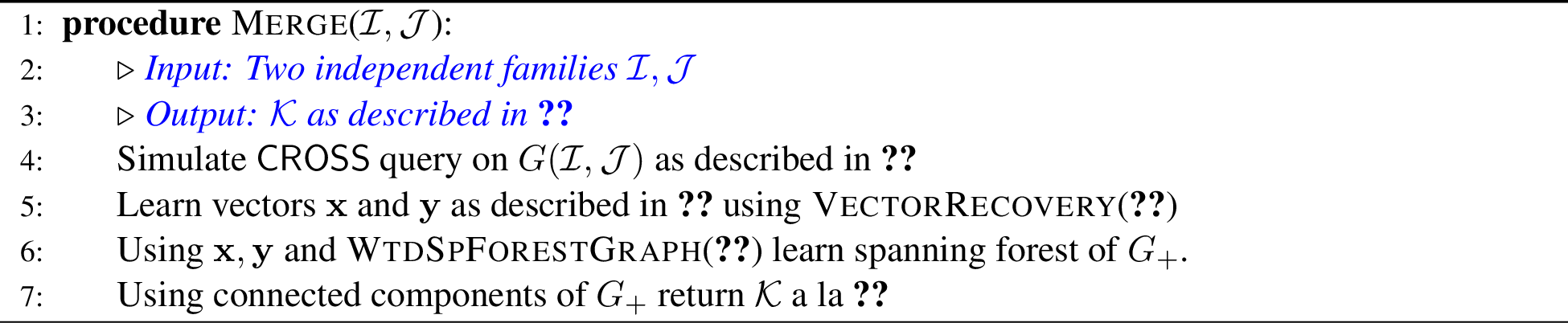
Lemma 7. Let \(\mathcal{I}\) and \(\mathcal{J}\) be two independent families, and let \(\mathcal{K}\) be the output of Merge(\(\mathcal{I}, \mathcal{J})\). Let \(d:= |\mathcal{I}| + |\mathcal{J}| - |\mathcal{K}|\). Merge, in expectation, makes \(O\left(\frac{d\log \max(|\mathcal{I}|, |\mathcal{J}|)}{\log d}\right)\) many \(\mathsf{CUT}\) queries.
Proof. The query complexity is dominated by VectorRecovery which makes (by 1)
\(O\left(\frac{d_\mathbf{x}\log s}{\log d_\mathbf{x}} + \frac{d_\mathbf{y}\log t}{\log d_\mathbf{y}}\right)\)-many queries (using 5). This is
in budget using 6. WtdSpForestGraph is randomized but the expected number of queries (2) is
\(O(d_\mathbf{x}+ d_\mathbf{y}) = O(d)\) by 6; since \(d \leq \max(s, t)\), this is also within budget. ◻
2.3 Connected Components in Hypergraphs↩︎
Given the Merge subroutine, we can complete the description of the full algorithm. As mentioned earlier, we always maintain a collection \(\mathfrak{I}:= (\mathcal{I}_1, \mathcal{I}_2, \ldots, \mathcal{I}_t)\) of independent families. We begin with \(t=n\) and initially \(\mathcal{I}_j\) contains a single, trivial supervertex \(\{v_j\}\). The algorithm proceeds in iterations, and in each iteration, we pick two independent families of nearly equal size and merge them. When we can’t do so any more, we have independent families of differing sizes, and so there can be only \(O(\log n)\) many families. In this case, we can just sequentially merge them again. The algorithm pseudocode is below.
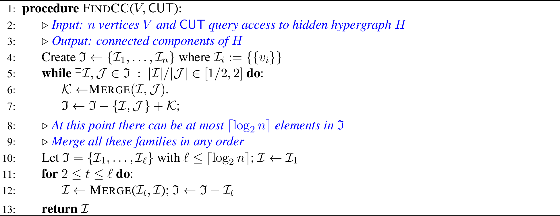
The correctness of the algorithm follows from the correctness of Merge. We now show that the total number of \(\mathsf{CUT}\) queries made is \(O(n)\) in expectation. Note that all queries are made in the Merge calls in Line [alg:q1] and Line [alg:q2]. We treat these separately.
Queries made in Line [alg:q1]. Recall that we use \(d:= |\mathcal{I}| + |\mathcal{J}| - |\mathcal{K}|\); without loss of generality, let us assume \(|\mathcal{I}| \geq |\mathcal{J}|\); note \(|\mathcal{I}| \le 2|\mathcal{J}|\). We call a \(\mathcal{K}\leftarrow\) Merge(\(\mathcal{I}, \mathcal{J})\) operation thick if \(d \geq \sqrt{|\mathcal{I}|}\). Otherwise, we call a Merge operation thin. By 7, the expected number of queries made by a thick Merge\((\mathcal{I}, \mathcal{J})\) is \(O\left(\frac{d\log |\mathcal{I}|}{\log d}\right)\) which is \(O(d)\) since the denominator cancels the logarithmic term in the numerator. Furthermore, consider the potential \(\Phi(\mathfrak{I}) := \sum_{\mathcal{I}\in \mathfrak{I}} |\mathcal{I}|\); a Merge drops \(\Phi(\mathfrak{I})\) by exactly \(d\). So all thick merges can be charged to, up to a multiplicative constant factor, to the total drop of \(\Phi(\mathfrak{I})\). In the beginning \(\Phi = n\), and so, the total query complexity, in expectation, of all thick merges is \(O(n)\). To address thin merges, we call an independent family \(\mathcal{I}\) to be in class \(t\) if \(|\mathcal{I}| \in [2^t, 2^{t+1})\), and classify a thin Merge(\(\mathcal{I}, \mathcal{J}\)) to be in class \(t\) if \(\min(|\mathcal{I}|, |\mathcal{J}|)\) is a class \(t\) family. Note that after such a thin merge, we replace \(\mathcal{I}\) and \(\mathcal{J}\) by \(\mathcal{K}\) with \(|\mathcal{K}| \geq 2^{t+1} - 2^{t/2}\). Thus \(\mathcal{K}\) is almost not in class \(t\). More precisely, let’s say a vertex \(v \in V\) participates in a class \(t\) merge if it is present in some supervertex of \(\mathcal{I}\) or \(\mathcal{J}\). What the above calculation shows is that the same vertex cannot participate in three class \(t\)-thin merges; the second class \(t\) merge would put \(v\) in an independent set which is in class \(t+1\) or higher. As a result, we can assert that the number of class \(t\)-thin merges is \(\leq \frac{2n}{2^t}\).
By 7, a class \(t\)-thin merge takes, in expectation, at most \(O\left(\frac{d\log (2^{t+1})}{\log d}\right)\) many \(\mathsf{CUT}\) queries. Since \(\frac{d}{\log d}\) is an increasing function of \(d\), and \(d = O(2^{t/2})\) since the merge is thin, the number of expected queries is at most \(O\left(\frac{2^{t/2}\log (2^{t+1})}{\log 2^{t/2}}\right) = O(2^{t/2})\). Combining with the upper bound on the number of class \(t\)-thin merges, we get that the total expected number of CUT queries made over thin merges is at most \(\sum_{t=0}^{{\left\lfloor{\log_2 n}\right\rfloor}} \frac{2n}{2^t} \cdot O(2^{t/2}) = O(n)\).
Queries made in Line [alg:q2]. We leverage the fact that the number of Merges is \(O(\log n)\). In particular, let \(d_t\) denote the drop \(|\mathcal{I}| + |\mathcal{I}_t| - |\mathcal{I}_{\mathrm{new}}|\) at the \(t\)th for-loop. Again by 7, the expected number of queries is at most \(O\left(\frac{d_t \log n}{\log d_t}\right)\), and so the total number of queries made in [alg:q2] is \(\sum_{t=1}^\ell \frac{d_t \log n}{\log d_t}\). Now, when \(\ell = O(\log n)\), one can show that \(\sum_{t=1}^\ell \frac{d_t}{\log d_t} \leq O(n/\log n)\). Indeed, if \(d_t \leq \frac{n}{\log^2 n}\), then we use the number of \(t\)’s is \(O(\log n)\) to bound their contribution to the sum by \(O(n/\log n)\). If \(d_t > \frac{n}{\log^2 n}\), then \(\frac{d_t}{\log d_t} = O(d_t/\log n)\) and so their contribution is at most \(O(\frac{\sum_t d_t}{\log n})\). Once again \(\sum_t d_t\) can be charged to \(\Phi(\mathfrak{I})\) initially which is \(n\). All in all, we get the following theorem which establishes 1.
Theorem 1. 2 returns the connected components of a hypergraph in an expected \(O(n)\) many \(\mathsf{CUT}\) queries.
3 Learning & Sparse Connectivity Certificates for Classes of Hypergraphs↩︎
As noted in the introduction, in general a hypergraph cannot be learned from \(\mathsf{CUT}\) queries since there are distinct hypergraphs with the same cut-profile. In this section, we show that this impossibility result is rather delicate and depends on the parity of the sizes of the hyperedges! In particular, if all the hyperedges are even, then we can learn the hypergraph using \(\mathsf{CUT}\) queries; there is no ambiguity.
Theorem 2. If \(H = (V, \mathcal{E})\) is a hypergraph with \(|e|\) an even* number for all \(e\in \mathcal{E}\), then we can efficiently learn \(H\) in \(O(\sum_{e\in \mathcal{E}} 2^{|e|}\cdot \log n)\) many \(\mathsf{CUT}\)-queries. If \(H\) was furthermore \(r\)-bounded, that is, \(|e|\leq r\) for all \(e\in \mathcal{E}\), then the query complexity is \(O(2^rm\log n)\) where \(m\) is the number of hyperedges.*
Indeed, we can say more underscoring the delicateness of the “reconstruction impossibility” even more. Suppose we also had access to a Boolean oracle \(\mathsf{EDGE^?}(S)\) which said True if \(S\in \mathcal{E}\) and False otherwise. This is similar to “pair” queries in a normal graph where given a pair one asks if it is an edge or not. Clearly, one can reconstruct an \(r\)-bounded hypergraph \(H\) using \(O(n^r)\) many \(\mathsf{EDGE^?}\)-queries. We can do much better when \(\mathsf{CUT}\) and \(\mathsf{EDGE^?}\) queries are given, and the hypergraph is sparse.
Theorem 3. Any hypergraph \(H = (V,\mathcal{E})\) with \(|V| = n\) and \(|\mathcal{E}| = m\) and \(|e|\leq r\) for all \(e\in \mathcal{E}\) can be reconstructed using \(O(2^r m\log n)\)-many \(\mathsf{CUT}\) queries and \(O(mn)\)-many \(\mathsf{EDGE^?}\)-queries.
The second class of hypergraphs which can be learned only using \(\mathsf{CUT}\) queries are linear hypergraphs. A hypergraph \(H = (V,\mathcal{E})\) is called linear if \(|e\cap f|\leq 1\) for any distinct \(e,f\in \mathcal{E}\). Note that this generalizes the notion of “simple” undirected graphs which states that between any two vertices, there can be at most one (hyper) edge. In general linear hypergraphs cannot be learned (see 4), but if \(|e|\geq 4\) for all \(e\in \mathcal{E}\), then we can learn it (even if it has edges with odd number of vertices).
Theorem 4. If \(H = (V, \mathcal{E})\) is a linear* hypergraph with \(|e| \geq 4\), then we can learn \(H\) in \(O(\sum_{e\in \mathcal{E}} |e|\log n) \leq O(n^2\log n)\) many \(\mathsf{CUT}\)-queries.*
3.0.0.1 Spanning Subhypergraphs and Sparse Certificates.
Given a hypergraph \(H = (V,\mathcal{E})\) with potentially parallel copies of a hyperedge, and a natural number \(k\), a sparse \(k\)-certificate (as in [16], [33], [34]) is a subhypergraph \(H' = (V, \mathcal{E}')\) with \(\mathcal{E}' \subseteq \mathcal{E}\) such that for any subset \(A\subseteq V\), we have \(|\partial_{H'}(A)| \geq \min(k, |\partial_{H}(A)|)\).
In particular, \(H'\) preserves all cuts up to size \(k\), and in particular, if the minimum cut of \(H\) is \(\leq k\), then so is the minimum cut in \(H'\). A \(1\)-sparse certificate is a spanning subhypergraph. The following result, essentially due to Nagamochi and Ibaraki [16] shows that if we have the ability to find spanning subhypergraphs, then we can construct \(k\)-sparse certificates by repeatedly finding and peeling.
Lemma 8 (Greedy Peeling a la Nagamochi-Ibaraki [16]). Given a hypergraph \(H = (V,\mathcal{E})\) on \(n\) vertices with potentially parallel copies of hyperedges, if we can find a spanning subhypergraph \(F \subseteq H\) in \(q(n)\) many \(\mathsf{CUT}\)-queries, then we can construct a \(k\)-sparse certificate in \(O(kq(n))\) many \(\mathsf{CUT}\)-queries.
Proof. This is a greedy peeling argument. If \(H_1, H_2, \ldots, H_k\) are subhypergraphs satisfying the property that \(H_i\) is a spanning hypergraph of \(H - \cup_{j=1}^{i-1} H_j\), then [16], [33], [34] show that \(\cup_{i=1}^k H_i\) is a \(k\)-sparse certificate. We refer the reader to these papers for this result. ◻
All our algorithms described above to learn hypergraphs proceed by learning “edge-by-edge”, and in particular, given a vertex \(x\) and a subset \(U\subseteq V\setminus x\), it can learn an edge incident to both \(x\) and \(U\). Using standard Prim-style algorithms, one can then learn a spanning subhypergraph. Using the above theorem, we can get sparse \(k\)-certificates. In particular, they give the following results.
Theorem 5. If \(H = (V, \mathcal{E})\) is a hypergraph with \(|e|\leq r\) an even* number for all \(e\in \mathcal{E}\), then we can efficiently construct a sparse \(k\)-certificate \(H\) in \(O(k2^rn\log n)\) many \(\mathsf{CUT}\)-queries.*
For linear hypergraphs, we can bypass the bounded hyperedge size condition when we construct sparse \(k\)-sparsifiers. This gives the following subquadratic guarantee for constant \(k\).
Theorem 6. If \(H=(V,\mathcal{E})\) is a linear* hypergraph, then we can find a cut-equivalent sparse \(k\)-certificate, not necessarily a subhypergraph of \(H\), in \(O(kn^{1.5}\log n)\) many \(\mathsf{CUT}\)-queries.*
3.1 Tools: Möbius Transform and Binary Search↩︎
Our algorithm to learn a hyperedge proceeds by learning it one vertex at a time. In particular, if \(e\) is an edge, and suppose we know a subset \(X\subseteq e\) of vertices of \(e\). To learn another vertex of \(e\), we would like a tool which answers a question of the following form: given a subset \(X\subseteq V\), does there exist a hyperedge \(e\) which contains all vertices of \(X\) and something outside? If we have such a tool, we can use a binary-search style technique to find the next vertex outside in \(O(\log n)\) calls. On the other hand, \(\mathsf{CUT}(X)\) counts the number of hyperedges which intersects some vertex of \(X\) and something outside. To get the former from \(\mathsf{CUT}\) queries, the idea is to look at the Möbius transform3 of the \(\mathsf{CUT}\)-function. Unfortunately, this tool doesn’t work all the time (as the impossibility results show), but when the parity is favorable, this idea goes through.
We begin with a few definitions.
Definition 1. Given a subset \(X\subseteq V\) and a non-empty \(A\subseteq V\setminus X\), define the functions
\(g(X; A) := \left\lvert \{e\in \mathcal{E}~:~ X\subseteq e, e\cap A \neq \emptyset, ~\textrm{and}~~e\cap V\setminus (X\cup A) \neq \emptyset\} \right\rvert\), and
\(h(X; A) := \left\lvert \{e\in \mathcal{E}~:~ X\subsetneq e, \textrm{and}~~e\subseteq A \cup X\} \right\rvert\).
In plain English, \(g(X;A)\) counts the number of hyperedges that contain all vertices of \(X\), intersects both \(A\) and \(V\setminus (A\cup X)\), while \(h(X;A)\) counts the hyperedges that contain all of \(X\), intersects \(A\), and is contained in \(A\cup X\) completely. So, \(g(X;A) + h(X;A)\) counts the number of hyperedges that contain all of \(X\) and touches some vertex of \(A\). Note that when \(A = V\setminus X\), this is precisely the tool described in the first paragraph. The next lemma shows that one can obtain some information depending on the parity of \(|X|\), and subsequently we show its utility.
Remark 1. Although we restrict our attention to unweighted hypergraphs, our reconstruction goes through for weighted hypergraphs with non-negative weights. For this, we need to modify the definition of \(g(X;A)\) and \(h(X;A)\) to be the total weight of the edges in the subset of their RHS instead of cardinality.
Lemma 9 (Möbius Transform). For a subset \(X\subseteq V\) and non-empty \(A\subseteq V\setminus X\), define \[\label{eq:qXA} Q(X; A) := \mathsf{CUT}(A) + \sum_{\emptyset \neq S\subseteq X} (-1)^{|S|+1}\left(\mathsf{CUT}(S) - \mathsf{CUT}(S\cup A)\right)\qquad{(1)}\] Then, we have \[Q(X;A) = \begin{cases} g(X; A) & \textrm{if |X| even} \\ g(X; A) + 2h(X;A) & \textrm{if |X| odd} \end{cases}\] Note that \(Q(X;A)\) can be computed in \(2^{|X|+1}\) many \(\mathsf{CUT}\)-queries.
We defer the proof of the above to 3.1.1 where we prove a generalization to subpartitions. We next show the utility of these queries.
Before that, we make a few observations.
Observation 1. Given disjoint subsets \(X\) and \(A\), if \(Q(X;A) > 0\), then this implies there exists an edge \(e\in \mathcal{E}\) such that \(X\subseteq e\) and \(e\cap A \neq \emptyset\) (irrespective of the parity of \(X\)). In particular, if \(A = \{a\}\), then \(X\cup \{a\}\subseteq e\). Furthermore, if \(|X|\) is odd, then it is an if-and-only-if statement. More precisely, if \(|X|\) is odd and \(Q(X;A) = 0\), then both \(g(X;A)\) and \(h(X;A)\) are \(0\) which means there is no edge \(e\) of the form \(X\subseteq e\) and \(e\cap A \neq \emptyset\).
Observation 2. Given disjoint subsets \(X\) and \(A\) and any partition \((A_1, A_2)\) of \(A\), we have \(Q(X;A) \leq Q(X;A_1) + Q(X;A_2)\)
Proof. One could obtain this via submodularity of \(\mathsf{CUT}\) in the definition ?? of \(Q(X;A)\), or one just uses 9 and the simpler-to-verify statements: \(g(X;A_1) + g(X;A_2) \geq g(X;A)\) and \(h(X;A_1) + h(X;A_2) \geq h(X;A)\). Indeed, any edge \(e\in \mathcal{E}\) counted in the RHS-es is either counted in the LHS or RHS, and any \(e\) intersecting both \(A_1\) and \(A_2\) are double counted in the LHS-es. ◻
Before we state our binary-search subroutine, we need one last standard fact.
Claim 1. Given any set \(A\) with \(|A| \geq 2\), there exists explicit partitions \((A^{(\ell)}_1, A^{(\ell)}_2)\) of \(A\) for \(1\leq \ell \leq {\left\lceil{\log_2 |A|}\right\rceil}\) with the property that for any distinct \(x,y \in A\), there is some \(\ell\) such that \(|A^{(\ell)}_1 \cap \{x,y\}| = |A^{(\ell)}_2 \cap \{x,y\}| = 1\). That is, \(x\) and \(y\) are split asunder in at least one of the partitions.
Proof. Index the elements of \(|A|\) as \({\left\lceil{\log_2|A|}\right\rceil}\)-dimensional bit-vectors, and define \(A^{(\ell)}_1 := \{x\in A: x_\ell = 1\}\) and \(A^{(\ell)}_2 = A\setminus A^{(\ell)}_1\). Any two \(x\) and \(y\) differ in at least one bit \(\ell\) and that suffices. ◻
Now we are ready to describe the binary search subroutine that uses the \(Q(X;A)\)’s.
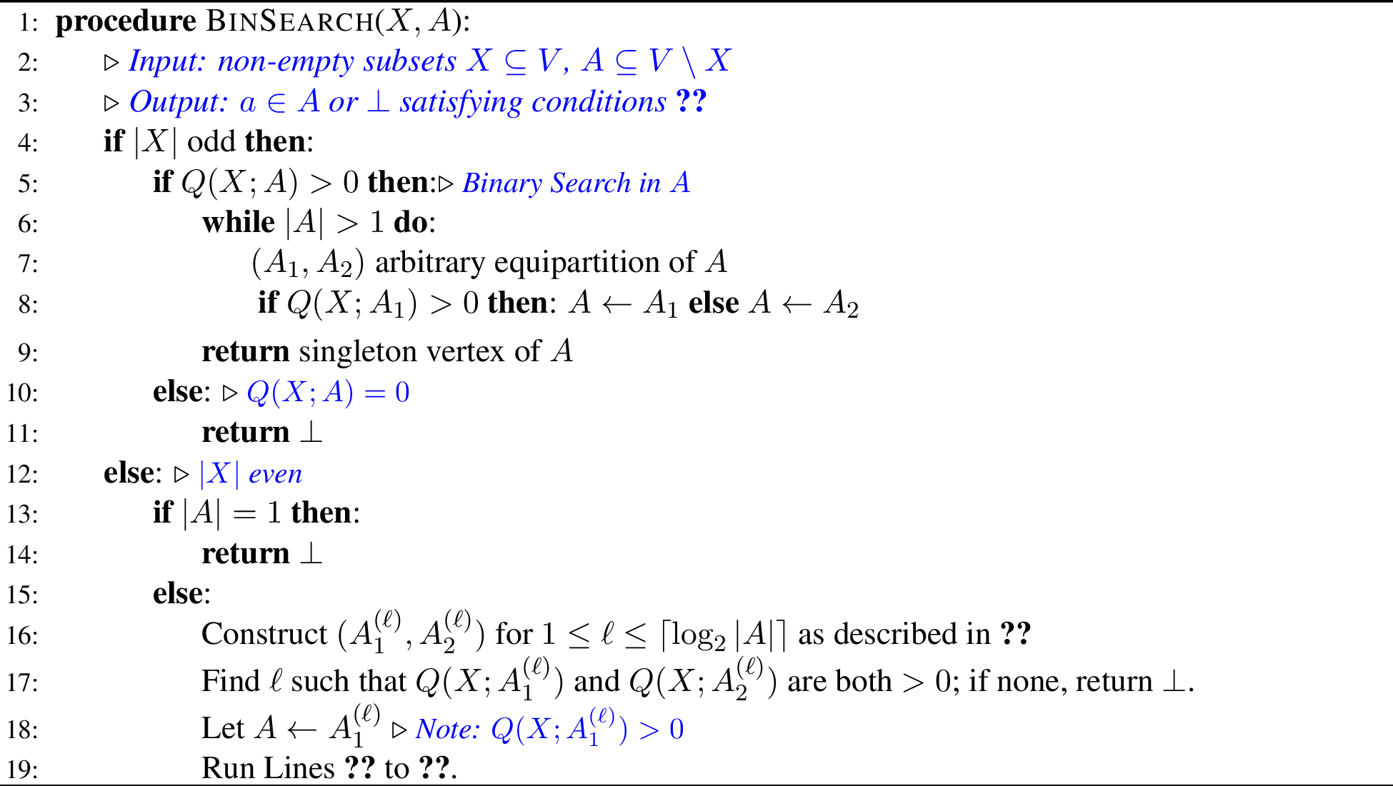
Lemma 10 (Spec of BinSearch(\(X,A\))). Let \(X\subseteq V\) and non-empty \(A\subseteq V\setminus X\) be two arbitrary subsets. Then,
when \(|X|\) is odd, BinSearch(\(X,A\)) either returns an \(a\in A\) such that there exists an edge \(e \in \mathcal{E}\) with \(X+a \subseteq e\), or it returns \(\bot\) and we can assert there is no* edge \(e\in \mathcal{E}\) such that \(X\subseteq e\) and \(|e\cap A| \geq 1\).*
when \(|X|\) is even, BinSearch(\(X,A\)) either returns an \(a\in A\) such that there exists an edge \(e \in \mathcal{E}\) with \(X+a \subseteq e\), or it returns \(\bot\) and we can assert there is no* edge \(e\in \mathcal{E}\) such that \(X\subseteq e\) and \(|e\cap A| \geq 2\).*
The algorithm makes \(O(\log n)\) many queries to \(Q(X;\cdot)\) and so can be simulated using \(O\left(2^{|X|+1}\log n\right)\) many \(\mathsf{CUT}\)-queries.
Proof. Let us consider the case when \(|X|\) is odd. We first query \(Q(X;A)\). If \(Q(X;A) = 0\), then by 1 we know there is no edge \(e\in \mathcal{E}\) with \(X\subseteq e\) and \(e\cap A \neq \emptyset\), and thus we return \(\bot\). Otherwise, we split \(A\) arbitrarily into \((A_1, A_2)\) such that each is of size \(\leq {\left\lceil{|A|/2}\right\rceil}\). By 2, we get \(Q(X;A) \leq Q(X;A_1) + Q(X;A_2)\), and so one of \(Q(X;A_1)\) or \(Q(X;A_2)\) is positive, and we recurse on that half. We continue so till we obtain a singleton vertex \(a \in A\) such that \(Q(X;\{a\}) > 0\). This means there is at least one edge \(e\in \mathcal{E}\) such that \(X\subseteq e\) and \(e\cap \{a\} \neq \emptyset\). In other words, \(X+a\subseteq e\).
Now let us consider the more interesting case when \(|X|\) is even. In this case \(Q(X;A) = 0\) doesn’t mean the non-existence of an edge “extending” \(X\). However, if there exists an edge \(e\in \mathcal{E}\) such that \(X\subseteq e\) and \(|e\cap A| \geq 2\). Then using 1, there is an \(1\leq \ell \leq {\left\lceil{\log_2|A|}\right\rceil}\) such that \(e\cap A^{(\ell)}_1 \neq \emptyset\) and \(e\cap A^{(\ell)}_2\neq \emptyset\). That is, \(g(X;A^{(\ell)}_i) > 0\) for \(i\in \{1,2\}\). Since \(|X|\) is even, we have \(Q(X;A^{(\ell)}_i) > 0\) for \(i\in \{1,2\}\). Contrapositively, if this isn’t true, then we can assert the non-existence of any edge \(e\in \mathcal{E}\) such that \(X\subseteq e\) and \(|e\cap A| \geq 2\). This is what we do in Line [line:bot2] by returning \(\bot\). Once we get our hand on such an \(\ell\), we then proceed as in the previous case to obtain an \(a\in A^{(\ell)}_1\) such that \(Q(X;\{a\})>0\), which, as in the previous case, implies the existence of the edge \(e\) with \(X+a\subseteq e\). ◻
The last preliminary observation is that once we find an edge \(e\in H\), we can simulate \(\mathsf{CUT}\)-queries on the hypergraph \(H' := H - e\). This is simply noting that \(\mathsf{CUT}_{H'}(S) = \mathsf{CUT}_H(S) - 1\) if \(e\cap S\) and \(e\cap V\setminus S\) are both non-empty, and equals to \(\mathsf{CUT}_H(S)\) otherwise. We can repeat this for any subset of edges.
Observation 3. If \(F\subseteq \mathcal{E}\) of a hypergraph \(H\), and if \(H' := H(V, \mathcal{E}\setminus F)\), then we can simulate \(\mathsf{CUT}_{H'}(\cdot)\) using \(\mathsf{CUT}_H(\cdot)\) and the knowledge of \(F\).
3.1.1 Proof of Lemma 9↩︎
We prove a generalization of 9. To that end, consider the following generalization of 1.
Definition 2. Let \(\mathcal{X}:= \{X_1, \ldots, X_t\}\) be a sub-partition of \(V\) and let \(Y := V \setminus \left(X_1\cup \cdots \cup X_t\right)\). Define \[g(\mathcal{X}) := \left\lvert \{e\in \mathcal{E}: e\cap X_i \neq \emptyset \forall i,~~e\cap Y\neq \emptyset\} \right\rvert~~\text{and}~~h(\mathcal{X}) := \left\lvert \{e\in \mathcal{E}: e\cap X_i \neq \emptyset \forall i,~~ e\cap Y = \emptyset\} \right\rvert\]
The above definition generalizes \(g(X;A)\) and \(h(X;A)\). Consider the partition \(\mathcal{X}_{X,A} := \{\{x\}~:~x\in X\} \cup \{A\}\). Then, first observe that \[g(X;A) = g(\mathcal{X}_{X,A})~~~\text{and}~~~h(X;A) = h(\mathcal{X}_{X,A})\] since \(e\cap \{x\} \neq \emptyset\) is the same as \(x\in e\). Secondly, observe that the RHS in ?? in the lemma below for \(\mathcal{X}= \mathcal{X}_{X,A}\) corresponds to the RHS in ?? . This can be seen by pairing the subfamily \(\mathcal{S}\) consisting only of singletons with \(\mathcal{S}\cup \{A\}\), which changes the parity leading to a term such as \(\mathsf{CUT}(S) - \mathsf{CUT}(S\cup A)\).
Lemma 11 (Generalized Möbius Transform). For any subpartition \(\mathcal{X}= (X_1, \ldots, X_t)\), define \[\label{eq:qXA-em} Q(\mathcal{X}) := \sum_{\emptyset \neq \mathcal{S}\subseteq \mathcal{X}} (-1)^{|\mathcal{S}|+1}~\cdot \underbrace{\mathsf{CUT}\left(\bigcup_{S\in \mathcal{S}} S\right)}_{\text{call this}~\mathsf{CUT}(\mathcal{S})~\text{for brevity}}\qquad{(2)}\] Then, we have \[Q(\mathcal{X}) = \begin{cases} g(\mathcal{X}) & \textrm{if |\mathcal{X}| odd} \\ g(\mathcal{X}) + 2h(\mathcal{X}) & \textrm{if |\mathcal{X}| even} \end{cases}\] Note that \(Q(\mathcal{X})\) can be computed in \(2^{|\mathcal{X}|+1}\) many \(\mathsf{CUT}\)-queries.
Proof. Given a subpartition \(\mathcal{P}\) of \(V\), we say \(e \cap \mathcal{P}= \emptyset\) if \(e\cap P=\emptyset\) for all \(P\in \mathcal{P}\).
Fix an edge \(e\in \mathcal{E}\). If \(e \cap \mathcal{X}= \emptyset\) it doesn’t participate in any of the terms in the RHS of the definition of \(Q(\mathcal{X})\). If \(e\cap \mathcal{X}\neq \emptyset\) but there is an \(X \in \mathcal{X}\) with \(e\cap X = \emptyset\), then for any \(\emptyset \neq \mathcal{S}\subseteq \mathcal{X}\) such that \(e\) contributes to \(\mathsf{CUT}(\mathcal{S})\), \(e\) also contributes with a different parity to \(\mathsf{CUT}(\mathcal{S}\cup \{X\})\), and thus cancels out. So the only \(e\)’s that survive are ones which intersect all \(X\in \mathcal{X}\); these are the \(e\)’s either counted in \(g(\mathcal{X})\) or \(h(\mathcal{X})\).
Now, let \(Y:= V\setminus \left(\bigcup_{X\in \mathcal{X}} X\right)\). If \(e\cap Y \neq \emptyset\), then it is counted in the RHS exactly \(\sum_{\emptyset \neq \mathcal{S}\subseteq \mathcal{X}} \left(-1\right)^{|\mathcal{S}|+1} = 1\) times; this is because of the cancellations of the binomial coefficients except the empty set. Thus, all edges contributing to \(g(\mathcal{X})\) are counted exactly once. If \(e\cap Y = \emptyset\), then the contribution of \(e\) to the RHS is precisely \(\sum_{\emptyset \neq \mathcal{S}\subseteq \mathcal{X}; \mathcal{S}\neq \mathcal{X}} \left(-1\right)^{|\mathcal{S}|+1}\) and this is \(0\) if \(|\mathcal{X}|\) is odd and \(2\) if \(|\mathcal{X}|\) is even. This implies a contribution of \(2h(\mathcal{X})\) when \(|\mathcal{X}|\) is even, completing the proof of the lemma. ◻
3.2 Even Hypergraphs↩︎
Armed with 10, we can prove the following lemma which, using 3, immediately proves 2.
Lemma 12. If \(H=(V,\mathcal{E})\) is a hypergraph with \(|e|\) even for all hyperedges, then given any \(x\in V\) and \(A\subseteq V\setminus x\), there is an algorithm which either decides there is no edge containing \(x\) which intersects \(A\), or returns an edge \(e\) with \(x\in e\) and \(e\cap A \neq \emptyset\). The number of \(\mathsf{CUT}\) queries made is \(O(2^{|e|}\log n)\).
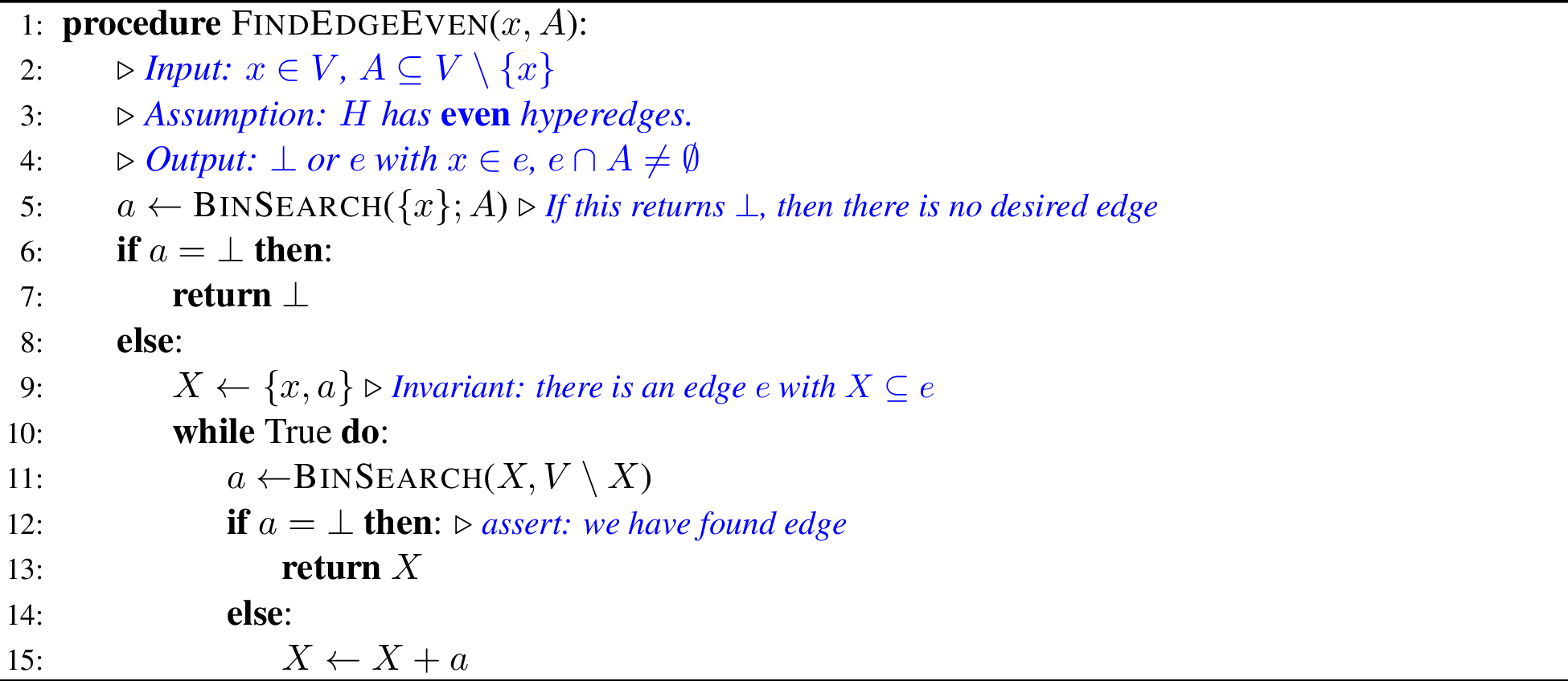
Proof. The algorithm is described in 4. We begin with BinSearch(\(\{x\};A\)); since \(|\{x\}|\) is odd, 10 implies that if this is \(\bot\), there is no edge containing \(x\) and intersecting \(A\), in which case we return \(\bot\). Otherwise, BinSearch returns an \(a\in A\) with the guarantee there is an edge \(e \supseteq \{x,a\}\). We now need to find the remaining vertices of one such edge. We let \(X = \{x,a\}\). Since we already found one \(a\in A\), we run our binary search BinSearch(\(X, V\setminus X)\). Since \(e\) has even sized, we know that either \(e = X\) or \(|e\cap (V\setminus X)| \geq 2\). This will in general be true; if \(|X|\) is even and there is an edge \(e\supseteq X\), then since \(|e|\) is even, either \(e = X\) or \(|e\cap (V\setminus X)| \geq 2\). This proves the correctness of Line [line:return]. When \(|X|\) is odd, then BinSearch\((X, V\setminus X)\) will not return \(\bot\). The total number of \(\mathsf{CUT}\) queries made is \(O\left(\sum_{i=1}^{|e|}2^i \cdot \log n\right)\) which evaluates to \(O(2^{|e|}\log n)\). ◻
If we also had the ability to make \(\mathsf{EDGE^?}\) queries, then before running Line [line:return], if \(|X|\) is even, we would actually check \(\mathsf{EDGE^?}(X\cup y)\) for all \(y\in V\setminus X\). If any of them return TRUE, then we return that edge. Otherwise, we return \(X\). This is correct because BinSearch(\(X,V\setminus X) = \bot\) implies there is no edge \(e\) with \(X\subseteq e\) and \(|e\cap (V\setminus X)| \geq 2\). However, the invariant is that there is an edge with \(X\subseteq e\). So either \(e = X\) or \(e = X + y\) for some \(y\in V\setminus X\). So the above algorithm works in any hypergraph but with \(n\) additional \(\mathsf{EDGE^?}\) queries. This immediately proves 3.
Armed with the above algorithm, we can easily find a spanning subhypergraph using a Prim-style approach described in 5.
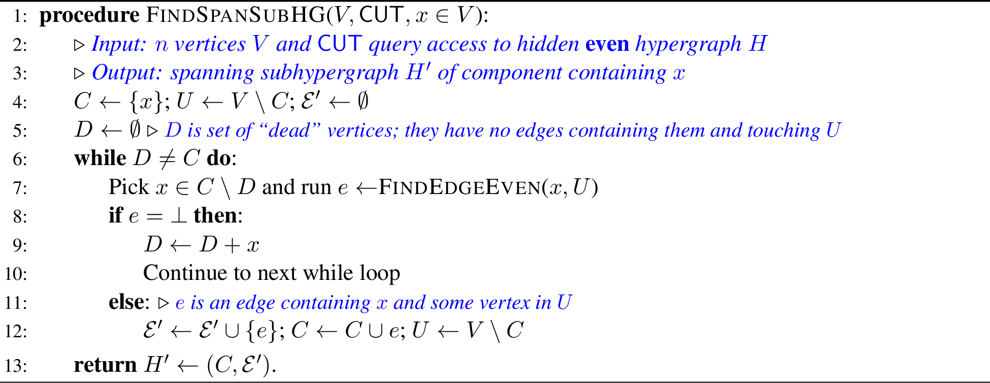
The time taken is \(O(\sum_{e\in \mathcal{E}'} 2^{|e|}\log n)\); if \(|e|\leq r\), then since \(|\mathcal{E}'| \leq n-1\), we obtain the spanning sub-hypergraph in \(O(2^r n\log n)\) many \(\mathsf{CUT}\) queries. Along with 8, this establishes 5.
3.3 Linear Hypergraphs↩︎
Recall, a hypergraph \(H = (V, \mathcal{E})\) is linear if for any two different \(e,f \in \mathcal{E}\), we have \(|e\cap f|\leq 1\). Furthermore, let us call a hypergraph large if \(|e| \geq 4\) for every \(e\in \mathcal{E}\). We first show that large, linear hypergraphs can be reconstructed easily. The main place where linearity is used is the following: if we know there exists an edge \(e\) such that \(\{x,y\} \subseteq e\), then there is exactly one such edge \(e^*\). So, if we find that there is an edge \(e\) containing \(\{x,y,z\}\), it must be the same edge \(e^*\); if we find there is an edge \(e\) containing \(\{x,y,z'\}\), it must be the same edge \(e^*\). The algorithm is now clear. Since \(|e^*|\geq 4\), we first use 10 with \(X=\{x,y\}\) and \(A=V\setminus X\) to find a vertex \(z\) with \(\{x,y,z\}\subseteq e^*\). We then fix the odd anchor \(X:=\{x,y,z\}\). Repeatedly applying 10 to \((X,A)\) finds all remaining vertices of the unique edge containing \(X\); uniqueness follows from linearity. When the search returns \(\bot\), there is no further vertex of that edge. The full description of the algorithm is in 6.
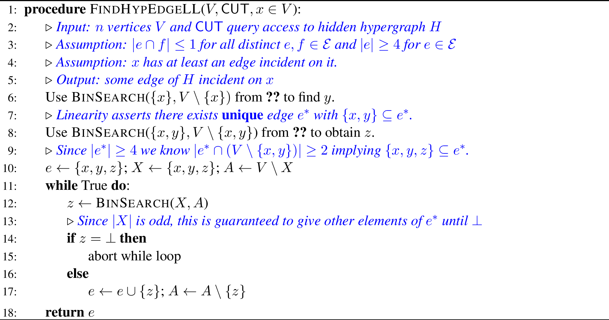
Remark 2. The above algorithm also works if \(|e|=2\) or \(|e| \geq 4\) for every \(e\in \mathcal{E}\). The only difference is that Line 8 of 6 may return \(\bot\) in which case \(\{x,y\}\) is the unique \(2\)-edge \(e^*\) containing both \(x\) and \(y\).
Since the size of \(|X|\) for which \(Q(X;A)\) is called is always \(\leq 3\), the above algorithm makes \(O(|e^*|\log n)\)-many \(\mathsf{CUT}\) queries. Armed with 3 (and noting that deleting an edge from a large, linear hypergraph maintains those properties), we obtain an algorithm which reconstructs all the edges in \(O(\sum_{e\in \mathcal{E}} |e| \cdot \log n)\) many \(\mathsf{CUT}\) queries, proving 4. To obtain a spanning subhypergraph, we use the same “Prim-style” ideas as employed in 5. The following claim relates the “size” \(p_H\) of linear hypergraphs.
Claim 2 (Size of Linear Hypergraphs). If \(H = (V, \mathcal{E})\) is a linear hypergraph with \(n = |V|\), \(m = |\mathcal{E}|\) and \(p = \sum_{e\in \mathcal{E}} |e|\), then (i) \(m \leq \binom{n}{2}\), and (ii) \(p = O(n\sqrt{m}) = O(n^2)\).
Proof. If we count the set \(\{(x,y,e): x\in V, y\in V, e\in \mathcal{E}, \{x,y\}\subseteq e\}\) and use linearity, we get that \(\sum_{e\in \mathcal{E}} \binom{|e|}{2} \leq \binom{n}{2}\). The LHS is at least \(|\mathcal{E}| = m\) proving (i). Cauchy-Schwarz proves (ii) since the aforementioned inequality implies \(\sum_{e\in \mathcal{E}} |e|^2 = O(n^2)\), and is at least \(p^2/m\). ◻
A spanning subhypergraph \(H'\) has at most \(n\) edges, and thus \(p_{H'} = O(n^{1.5})\) showing that we can find a spanning subhypergraph in a large, linear hypergraph in \(O(n^{1.5}\log n)\)-many \(\mathsf{CUT}\) queries. Next, we discuss how to remove the largeness assumption. Before moving on to do so, we state the obvious generalization which may be of interest: it weakens the linearity to \(t\)-linearity, but then requires all edges to be much bigger; one uses Hölder instead of Cauchy-Schwarz.
Theorem 7. For any \(t \in \mathbb{N}\), if a hypergraph \(H = (V,\mathcal{E})\) satisfies (i) \(|e|\geq t+3\) for all \(e\in \mathcal{E}\), and (ii) \(|e\cap f| \leq t\) for all distinct \(e,f\in E\), then a spanning subhypergraph can be learned in \(O(n^{2 - \frac{1}{(t+1)}}\log n)\)-many \(\mathsf{CUT}\)-queries.
3.3.0.1 Removing the largeness assumption.
From the above discussion, we can see that one could learn all large hyperedges, but one is stuck at edges \(e\) with \(|e| \leq 3\). And indeed, as noted in 1, one cannot exploit linearity to learn the hypergraph exactly. However, one other simple observation still allows us to construct “sparse certificates” — we put quotes because we won’t be able to find \(3\)-edges of \(H\) – but we don’t need to; a triangle is the same as three normal edges with “half” the weight.
Observation 4. Let \(H = (V,\mathcal{E})\) be any hypergraph. Construct \(\widetilde{H}= (V,\widetilde{\mathcal{E}})\) which is a hypergraph formed as follows: for each \(e\in \mathcal{E}\) with \(|e| = 2\) or \(|e|\geq 4\), we add two* copies of \(e\) to \(\widetilde{\mathcal{E}}\), and for \(e = \{a,b,c\}\) in \(\mathcal{E}\), we add \((a,b), (b,c)\) and \((c,a)\) to \(\widetilde{\mathcal{E}}\). Then, for any \(S\subseteq V\), \(\mathsf{CUT}_{\widetilde{H}}(S) = 2\mathsf{CUT}_H(S)\). That is, \(\widetilde{H}\) and \(2H\) are cut-equivalent. Furthermore, given any \(\widetilde{e} \in \widetilde{\mathcal{E}}\), one can simulate \(\mathsf{CUT}_{\widetilde{H}- \widetilde{e}}(S)\) as \(2\mathsf{CUT}_H(S) - 1\) if \(S\cap e \neq \emptyset\) and \((V\setminus S) \cap e \neq \emptyset\), and \(2\mathsf{CUT}_H(S)\) otherwise.*
Since \(\mathsf{CUT}()\) is additive over the hyperedges, it suffices to argue for a single edge \(e \in H\) with \(|e| = 3\). Now one can check this brute-force; the main reason is that any relevant cut looks the same: one vertex of \(e\) on one side and two on the other. This is, unfortunately, particular to \(|e| = 3\), and we are not able to generalize to \(|e| = 5\) or other odd hyperedges. More precisely, if we could replace all odd-sized hyperedges with even-sized hyperedges and be cut-equivalent, then we would be able to generalize 2 to all bounded hypergraphs.
Armed with the above observation, we can obtain 3 as follows. We assume we are working with \(\widetilde{H}\) and since there are no \(|e| = 3\), 6 (or rather its spanning subhypergraph version) will find a spanning subhypergraph \(H_1\) of \(H\) in \(O(n^{1.5}\log n)\) many \(\mathsf{CUT}\) queries. Therefore, we can apply 8 to find \(H_1, \ldots, H_{2k}\) such that their union is a \(2k\)-sparse certificate of \(\widetilde{H}\). Since \(\widetilde{H}\) and \(2H\) are cut-equivalent, this union is a \(k\)-sparse certificate (but not a subhypergraph) of \(H\). 3 is established fully by noting that in \(O(n^2\log n)\) many \(\mathsf{CUT}\)-queries, we can learn all of \(\widetilde{H}\).
4 Odd Hypergraphs with Same Cut Profile↩︎
In this section we show that odd parity of cardinality of edges is a key hindrance to learning hypergraphs. In particular, we prove the following theorem.
Theorem 8. Let \(k\geq 3\) be an odd number. There are two \(k\)-uniform hypergraphs \(H_0\) and \(H_1\) on the same labeled vertex set \(V\) whose cut-profiles are the same.
Proof. The vertex set \(V\) has \(2k\) vertices named \(v_1, \ldots, v_k\) and \(\overline{v}_1, \ldots, \overline{v}_k\). The set of edges \(e\in H_0\) (and in \(\in H_1\), respectively) are all subsets of \(V\) such that \(e\) contains exactly one vertex from \(\{v_i, \overline{v}_i\}\) for \(1\leq i\leq k\) and the number of \(\overline{v}_i\)’s is even (respectively, odd). Thus, every edge has exactly \(k\) vertices. The number of edges in \(H_0\) is \(\sum_{0\leq i\leq k: i~\text{even}} \binom{k}{i}\) and the number of edges in \(H_1\) is \(\sum_{0\leq i\leq k: i~\text{odd}} \binom{k}{i}\). Since \(k\) is odd, both expressions are the same and equal to \(2^{k-1}\).
Let \(\mathsf{CUT}_0\) and \(\mathsf{CUT}_1\) be cut-functions in \(H_0\) and \(H_1\), respectively. We want to argue that \(\mathsf{CUT}_0(S) = \mathsf{CUT}_1(S)\) for any \(S\subseteq V\). It will be convenient to count the number of edges not counted in \(\mathsf{CUT}_i(S)\) for \(i\in \{0,1\}\); in particular, define \(g_i(S)\) to be the number of edges \(e\in E_i\) such that \(e\subseteq S\) or \(e\subseteq V\setminus S\). So, \(\mathsf{CUT}_i(S) = 2^{k-1} - g_i(S)\), and so it suffices to show \(g_0(S) = g_1(S)\).
Call \(S\) consistent if \(|S\cap \{v_i, \overline{v}_i\}| = 1\) for all \(1\leq i\leq k\). Define a map \(\phi_S : E(H_0) \to E(H_1)\) by flipping the bits as follows: for \(e\in E(H_0)\), we define \(\phi(e)\) to contain \(v_i\) if \(\overline{v}_i \in e\) or vice-versa. Note that if the number of “barred” vertices in \(e\) is \(j\), then the number of “barred vertices” in \(\phi_S(e)\) is \(k-j\). Since \(k\) is odd, we get that \(\phi_S(e) \in E(H_1)\). It is easy to see this is a bijection. Furthermore, note that \(e \subseteq S \Leftrightarrow \phi_S(e) \subseteq V\setminus S\) and \(e\subseteq V\setminus S \Leftrightarrow \phi_S(e) \subseteq S\). And so there is a bijection between the set of uncut edges proving \(g_0(S) = g_1(S)\) for consistent subsets.
Let \(S\) be an inconsistent subset, and let \(i\) be the smallest index such that \(\{v_i, \overline{v}_i\} \subseteq S\) (the case of \(\subseteq V\setminus S\) would be analogous.). Now note that no edge \(e\), either in \(H_0\) or \(H_1\), can be a subset of \(V\setminus S\) (in the analogous case, subset of \(S\)). Now, for \(e\in E(H_0)\), define \(\phi_S(e)\) to be the edge where the parity of \(v_i\) is flipped; that is, if \(v_i\in e\) then \(\overline{v}_i \in e\) and everything else remains the same. It is easy to see this is a bijection. Furthermore, if \(e\subseteq S\) then \(\phi_S(e) \subseteq S\). And this shows that \(g_0(S) = g_1(S)\) for such an inconsistent subset as well. This completes the proof. ◻
When \(k=3\), the above two hypergraphs are indeed linear; in fact, every pair of hyperedges intersect in exactly one vertex.