No title
January 01, 1970
Abstract
Sample-based generative models are increasingly used for probabilistic forecasting in high-stakes decision settings, yet their training objectives are blind to the decision maker’s cost structure. These models are commonly trained with strictly proper scoring rules, such as the energy score, which allocate their training signal in proportion to data density, with no awareness of where forecast errors are most costly for downstream decisions. We therefore propose decision-aware training for sample-based generative models, augmenting the energy score objective with a differentiable decision loss that directly penalises the cost incurred by acting on the model’s forecast. This combined loss is theoretically grounded, as the decision loss is itself a proper scoring rule. We validate our method on one synthetic and two real-world tasks, showing targeted improvements in cost-sensitive regions while retaining full probabilistic forecasts.
1 Introduction↩︎
Probabilistic forecasting models are increasingly deployed in high-stakes decision-making, for example, a wind farm operator committing to a power contract based on a wind forecast, risking costly shortfall penalties if they over-commit, or a farmer deciding whether to apply frost protection based on a temperature forecast, balancing asset loss against the cost of intervention. In the weather domain, state-of-the-art forecasting systems [1], [2] are trained with strictly proper scoring rules such as the energy score [3], which are uniquely minimised by the true conditional distribution. In practice, however, limited model capacity and empirical risk minimisation yield only local optimality [4], inducing tradeoffs between model error in different regions of the input/output space [5]: proper scoring rules distribute the training gradient in proportion to data density, with no awareness of the decision maker’s cost structure. The model’s limited capacity is allocated globally, leaving decision-critical regions of the output space potentially underserved.
Given a forecast, a decision maker with cost function \(c(a, y)\), of action \(a\) and outcome \(y\), selects the action that minimises expected cost under the forecast distribution; a point forecast is insufficient to evaluate this expectation. A good forecast should yield low expected costs when acted upon and correctly anticipate those costs, the latter property being known as decision calibration [6]. Crucially, the observed cost of the optimal action is itself a proper scoring rule [7], [8], placing it in the same family as the energy score which licenses their combination as a theoretically well-founded training objective for decision-aware training.
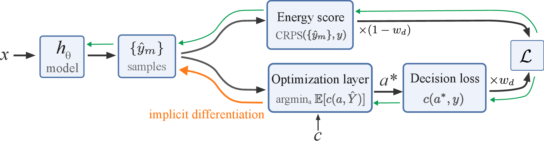
We augment the energy score with the optimal action cost as a differentiable decision loss. The decision loss alone is insufficient as a training objective: it only constrains the model in cost-sensitive regions, leaving the rest of the distribution unanchored and prone to degeneration. The energy score acts as that anchor, preventing the model from collapsing outside cost-sensitive regions. During training, samples drawn from the model are used to compute the optimal action \(a^*\) via a differentiable optimization layer; the decision loss then evaluates the cost incurred by \(a^*\) against the true outcome \(y\), and gradients flow back through \(a^*\) to the model parameters via implicit differentiation. Our method is theoretically grounded and leads to better downstream decisions while retaining full probabilistic forecasts, as validated on synthetic and real-world forecasting tasks.
Contributions.
An end-to-end decision-aware training framework for implicit generative models and distributional diffusion models, bridging decision-focused learning and probabilistic forecasting by retaining distributional accuracy via an energy score anchor.
A theoretically principled combination of decision loss and energy score, exploiting the equivalence between optimal action costs and proper scoring rules.
A gradient analysis showing which regions benefit from the decision loss and why, based on the cost function structure.
Empirical validation on synthetic and real-world forecasting tasks, evaluating both decision loss and decision calibration.
In the following, we start with summarising the necessary background in [sec:forecasting] [sec:decision] before introducing our method in 4 and validating it in 5.
2 Probabilistic Regression and Scoring Rules↩︎
We consider a probabilistic regression setting where input features \(X \in \mathcal{X}\) and target \(Y \in \mathcal{Y}\) are random variables distributed according to \(P_{X,Y}\). Given a realisation \(x\) of \(X\), the goal is to learn a model \(h_\theta\) that produces a predictive distribution \(\hat{F}_x = h_\theta(x)\) over \(Y\) which ideally recovers the true conditional \(Y \mid X = x\). We drop the subscript \(x\) throughout for brevity.
For this work, we consider two classes of sample-based generative models: implicit generative models, which map noise directly to samples, and distributional diffusion models, which generate samples via an iterative denoising process. Both represent \(\hat{F}_x\) implicitly via samples \(\{\hat{y}_m\}_{m=1}^M\). Implicit generative models [9] map a conditioning input \(x\) and a noise vector \(\varepsilon_m \sim \mathcal{N}(0, I)\) directly to a sample \(\hat{y}_m \sim \hat{F}_x\) via \(\hat{y}_m = f_\theta(x, \varepsilon_m)\); drawing \(M\) independent noise vectors in parallel yields \(M\) samples in a single forward pass. Diffusion models [10], [11] gradually add noise to the clean target \(y_0\) and learn a reverse denoising process conditioned on \(x\).1 At each reverse step, a denoiser estimates the clean target \(y_0\) from a noisy observation \(y_t\) and the conditioning input \(x\); in the standard formulation this prediction is a point estimate. Since \(y_0\) is genuinely uncertain given \((y_t, x)\), we consider the special class of distributional diffusion models [12], [13] whose denoiser models a full distribution over \(y_0\), from which samples can be drawn at each step. At inference, samples from \(\hat{F}\) are obtained by iterating the full reverse chain.
A scoring rule \(S(\hat{F}, y)\) assigns a scalar score to a predictive distribution \(\hat{F}\) given the realised outcome \(y\). It is proper if the true conditional \(F\) minimises the expected score, \(\mathbb{E}_{Y \sim F}[S(\hat{F}, Y)] \geq \mathbb{E}_{Y \sim F}[S(F, Y)]\) for all \(\hat{F}\), and strictly proper if \(F\) is the unique minimiser. The energy score (ES) [3] is a popular example of a strictly proper scoring rule that admits a sample-based estimator (see 8.1). For univariate targets the energy score reduces to the continuous ranked probability score (CRPS), widely used in meteorological forecast verification [14] and as a training objective for state-of-the-art ML weather prediction models [1], [2]. Both model classes introduced above are commonly trained by minimising strictly proper scoring rules, and in particular the energy score.
3 Decision-Making Under Uncertainty↩︎
Given a probabilistic forecast \(\hat{F}\) over \(\mathcal{Y}\), a decision maker selects an action \(a \in \mathcal{A}\) to minimise expected cost under the forecast. This is modelled via a cost function \(c : \mathcal{A} \times \mathcal{Y} \to \mathbb{R}\) that encodes the preferences of a particular decision maker; the Bayes-optimal action is \[\begin{align} a^*(\hat{F}) &\mathrel{\vcenter{:}}= \operatorname*{argmin}_{a \in \mathcal{A}} \, \mathbb{E}_{Y \sim \hat{F}}[c(a, Y)] \tag{1}\\ &\approx \operatorname*{argmin}_{a \in \mathcal{A}} \frac{1}{M}\sum_{m=1}^M c(a, \hat{y}_m)\eqqcolon a^*(\hat{F}_M) \tag{2}. \end{align}\] The expectation ensures that rare but sufficiently costly events still influence the optimal action. For sample-based models, the expectation is replaced by its Monte Carlo estimate over samples \(\{\hat{y}_m\}\), where \(\hat{F}_M\) denotes the empirical forecast distribution over \(\{\hat{y}_m\}\).
The realised cost when acting on forecast \(\hat{F}\) and observing the true outcome \(y\) is \(c(a^*(\hat{F}), y)\). A forecast is decision-calibrated [6] if its predicted expected cost matches the realised cost in expectation over inputs: \[\mathbb{E}_{X}\,\mathbb{E}_{Y \sim \hat{F}_X}\bigl[c(a^*(\hat{F}_X),\, Y)\bigr] = \mathbb{E}_{(X,Y)}\bigl[c(a^*(\hat{F}_X),\, Y)\bigr]. \label{eq:dec95calibration}\tag{3}\] Intuitively, that means a decision-calibrated model correctly anticipates the cost of its own optimal action. We measure decision miscalibration as the mean absolute difference between predicted cost and realised cost across test points \(\frac{1}{N} \sum_{i=1}^N \left| \mathbb{E}_{Y \sim \hat{F}_{x_i}}\bigl[c(a^*(\hat{F}_{x_i}), Y)\bigr] - c(a^*(\hat{F}_{x_i}), y_i) \right|\).
In principle, strictly proper scoring rules provide a path to optimal decisions: they guarantee convergence to \(F\) at the global optimum [3], and the true \(F\) yields optimal decisions by construction.2. In practice, however, limited data, model capacity, and stochastic optimisation yield only approximate local minima [4], with no awareness of where \(c\) is sensitive [5], so a model minimising the energy score may be decision-miscalibrated and incur high decision cost.
4 Decision-Aware Training↩︎
We address the gap between scoring-rule training and downstream decision quality by augmenting the scoring rule objective with a differentiable decision loss that directly penalises suboptimal decisions (1). We first establish the theoretical grounding and introduce the combined objective (4.1), then analyse the gradient chain through the optimal action (4.2), and describe the model architectures and training procedure (4.3).
4.1 Loss formulation and theoretical grounding↩︎
The decision problem of 3 suggests a natural training signal: directly penalise the cost incurred by the model’s optimal action at the realised outcome. We define the decision loss \[S_c(\hat{F}, y) = c\!\left(a^*(\hat{F}),\, y\right), \label{eq:dec95loss}\tag{4}\] where \(a^*(\hat{F})\) is the Bayes-optimal action in 1 . The key observation is that \(S_c\) is itself a proper scoring rule.
Proposition 1 (Hartline et al., 2025; Kleinberg et al., 2023). The decision loss \(S_c\) is a proper scoring rule: \(\mathbb{E}_{Y \sim F}[S_c(F, Y)] \leq \mathbb{E}_{Y \sim F}[S_c(\hat{F}, Y)]\) for all forecasts \(\hat{F}\). However, it is not strictly proper: there can be \(\hat{F} \neq F\) with \(a^*(\hat{F}) = a^*(F)\) that achieve the same minimum.
This means \(S_c\) is part of the same loss family as the energy score.3 However, since the minimum is not unique, optimising \(S_c\) alone admits degenerate solutions. The energy score provides the missing uniqueness: as a strictly proper scoring rule, it admits \(F\) as its unique minimiser, and a positive linear combination of a strictly proper and a proper scoring rule remains strictly proper (1, 8.2). This result directly applies to the training of sample-based generative models, offering a natural extension to the existing scoring rule training objective.
Combined loss. Hence, we define our loss as convex combination of energy score and decision loss \[\mathcal{L} = (1 - w_d)\,\mathrm{ES} + w_d\,S_c, \qquad w_d \in [0, 1), \label{eq:combined}\tag{5}\] with a unique minimum at \(\hat{F} = F\). The decision weight \(w_d\) controls the tradeoff between distributional accuracy and decision awareness. The energy score serves as a theoretical anchor, eliminating the degenerate solutions admitted by \(S_c\) alone, while \(S_c\) concentrates the gradient on the cost-relevant region. This combination yields a theoretically grounded objective that is both decision-aware and distribution preserving.
4.2 Optimizing the decision loss↩︎
Training with the decision loss \(S_c\) requires computing \(a^*\) from samples via 2 ; the backward pass must then differentiate \(a^*\) with respect to those samples. For general cost functions, \(a^*\) has no closed-form expression in the samples \(\{\hat{y}_m\}\), so we cannot differentiate it with respect to \(\{\hat{y}_m\}\) directly; instead we differentiate the optimality conditions that define \(a^*\) treating \(a^*\) as an implicit function of \(\{\hat{y}_m\}\) (implicit differentiation). We compute \(a^*\) within a differentiable optimization layer [5], [18], [19] over the feasible set \(\mathcal{A} = [a_\mathrm{min}, a_\mathrm{max}]\), treating model samples as fixed. This requires \(c\) to be differentiable in \(a\) and the expected cost in 1 to be strictly convex at \(a^*\), allowing implicit differentiation through \(a^*\).
The decision loss \(S_c = c(a^*, y_\mathrm{obs})\) depends on model parameters only through the samples \(\{\hat{y}_m\}\) and hence through \(a^*\). The gradient with respect to each sample is \[\frac{\partial S_c}{\partial \hat{y}_m} = \left.\frac{\partial c}{\partial a}\right|_{a^*} \cdot \frac{\partial a^*}{\partial \hat{y}_m}, \label{eq:grad95chain}\tag{6}\] where \(\partial a^* / \partial \hat{y}_m\) is obtained via implicit differentiation, whereas the remaining upstream gradient with respect to model parameters is computed via standard automatic differentiation.
Per-sample gradient. When \(a^* \in (a_\mathrm{min}, a_\mathrm{max})\), implicit differentiation gives \[\frac{\partial a^*}{\partial \hat{y}_m} = -\left[\frac{1}{M}\sum_{j=1}^M \frac{\partial^2 c}{\partial a^2}(a^*, \hat{y}_j)\right]^{-1} \frac{1}{M}\, \frac{\partial^2 c}{\partial a\, \partial \hat{y}_m}(a^*, \hat{y}_m). \label{eq:ift95member}\tag{7}\] The gradient signal is concentrated on samples \(\hat{y}_m\) where the cost has non-zero cross-curvature, \(\partial^2 c / \partial a \partial \hat{y}_m \neq 0\), i.e., where small perturbations of \(\hat{y}_m\) change how sensitive the cost is to \(a\); samples in flat or saturated cost regions contribute almost nothing (full derivation in 8.4). In parametric approaches (e.g.a Gaussian MLP), gradients update distribution parameters such as mean and variance, shifting the entire predictive distribution simultaneously. In our sample-based models, the noise input \(\varepsilon\) enables flexible distributional shapes and targeted corrections to specific parts of the predictive distribution even with shared weights. However, this flexibility can also lead to distributional degeneration at high \(w_d\) in practice.
Constraint boundary blocking. 7 applies when \(a^*\) is interior, where the first-order condition \(\nabla_a \mathbb{E}[c(a^*, \{\hat{y}_m\})] = 0\) holds. When \(a^*\) reaches a constraint boundary (\(a^* \in \{a_\mathrm{min}, a_\mathrm{max}\}\)), 7 does not apply. In this case the gradient is simply zero: geometrically, small perturbations of the samples do not move \(a^*\) off the boundary, so \(\partial a^*/\partial \hat{y}_m = 0\) (formal derivation via KKT conditions in 8.4), blocking the decision loss gradient chain in 6 entirely.4 The energy score is then the only active training signal.
4.3 Model architectures and training procedure↩︎
For this work, we consider two sample-based generative architectures representative of those used in operational forecasting systems. We extend both with a differentiable optimization layer that computes \(a^*\) from the model samples during training.
Implicit generative model. An MLP maps \(M\) independent noise draws to \(M\) samples in a single forward pass, from which \(a^*\) is computed. Architecture details are given in 9.
Distributional diffusion model. An MLP denoiser produces \(M\) samples of \(y_0\) at each denoising step, from which \(a*\) is computed. The decision loss acts at the denoiser level, while the predictive distribution \(\hat{F}_x\) at inference is shaped by iterating the full reverse chain, a second layer of sampling not present in the implicit generative model.
Training procedure. At each training step, the model is trained by optimising the combined loss (5 ). The model produces a set of samples \(\{\hat{y}_m\}_{m=1}^M\) for each input \(x\) in the batch. These samples enter both terms of the combined loss (1). First, the energy score (CRPS for univariate targets) is evaluated as usual (see Appendix 8.1), with gradients computed via standard autodiff. Second, \(a^*\) is computed by minimising the expected cost over the same samples (2 ) via the optimisation layer forward pass, treating the model samples as fixed. The decision loss \(S_c\) is then evaluated and its gradient flows back through \(a^*\) via implicit differentiation (4.2). In practice, both loss terms are estimated from finite \(M\) samples. Both losses are normalised to unit scale before training, so that \(w_d\) directly controls the relative weighting between the two terms independently of the cost function’s magnitude; further implementation details are given in 9.
5 Experiments↩︎
In the following we evaluate our method on one synthetic and two real-world decision tasks.
5.1 Synthetic Decision Task↩︎
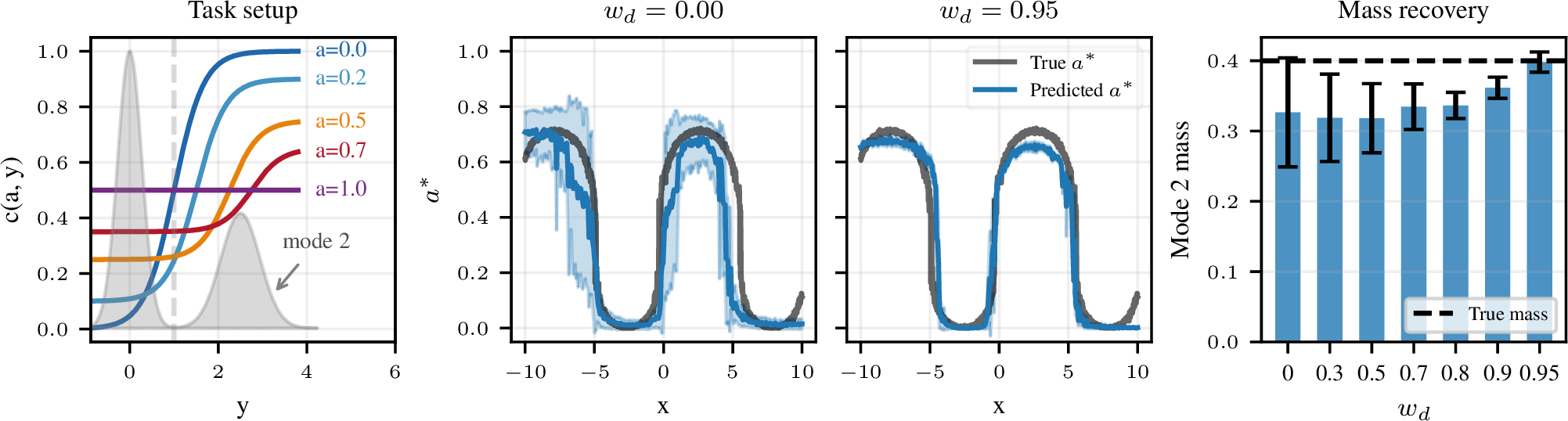
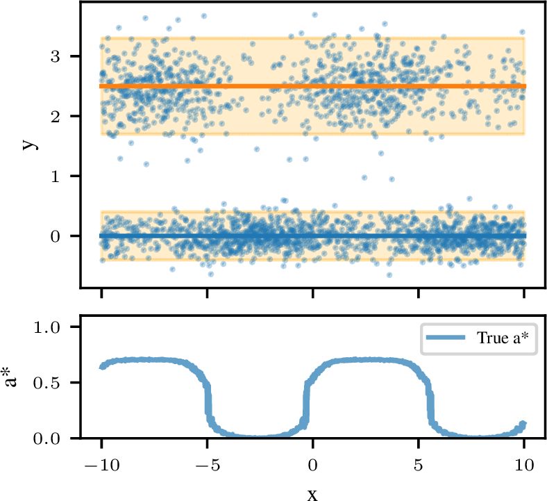
Setup. To study the mechanism underlying decision-aware training in a controlled setting where the ground-truth conditional distribution is known, we construct a synthetic dataset with the following structure. The target \(Y \mid X\) follows a bimodal Gaussian mixture distribution with fixed mode positions (\(\mu_1 = 0\), \(\mu_2 = 2.5\)), fixed standard deviations (\(\sigma_1 = 0.2\), \(\sigma_2 = 0.4\)), but a sinusoidally varying mixture weight \(w(x)\), with mode 2 (the right mode at \(y = 2.5\) in 2 left) having lower marginal weight \(0.4\). The decision maker must choose a protection level \(a \in [0, 1]\) against a hazard concentrated above a threshold at \(y = 1.0\) (between the two modes): higher \(a\) reduces exposure to the hazard but incurs a growing protection cost. The threshold is set so that the mixture weight \(w(x)\) is the key determinant of the optimal action and mode-weight tracking, thus the key diagnostic. We train a distributional diffusion model on this task across multiple data and training seeds; details are in 10.1.
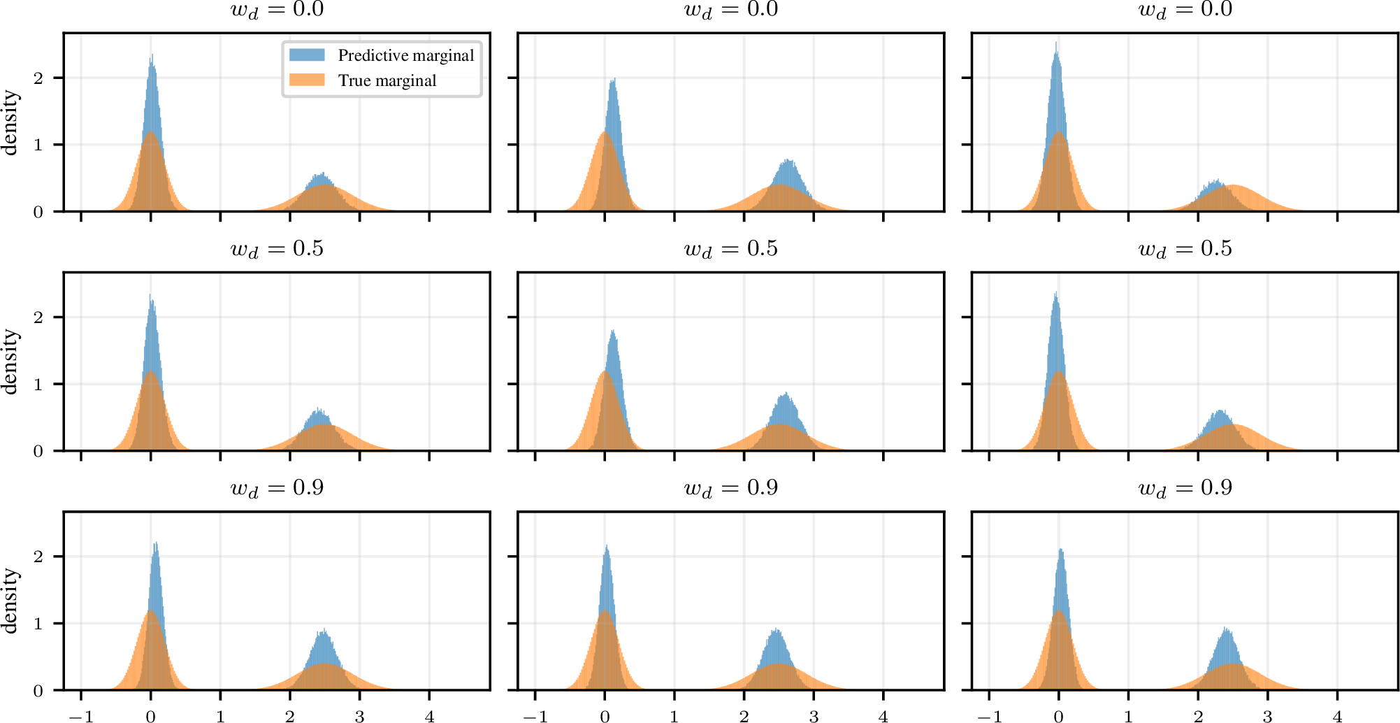
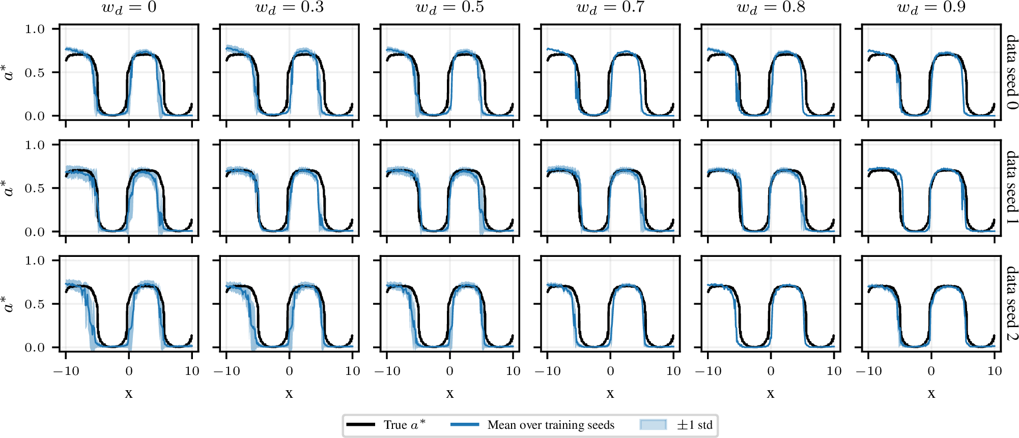
Results. With this setup in place, we first ask whether a standard proper scoring rule suffices. Under pure CRPS training (\(w_d=0)\), the diffusion model roughly captures the extreme values of \(a^*(x)\) but fails to reproduce the sinusoidal transitions of \(a^*\) between extremes, reflecting inaccurate mode weight tracking across \(x\) (2). Inspecting the mode weights of the marginal predictive distributions shows that the costly mode (mode 2 in 2) is systematically underweighted when trained with CRPS alone (\(w_d=0\)).
Adding the decision loss directly addresses this: as the decision weight \(w_d\) increases, the predicted \(a^*(x)\) tracks the ground truth more closely, with larger improvements at higher \(w_d\), consistently across data seeds (2). The marginal mode weights are progressively corrected as \(w_d\) increases, with probability mass shifting toward mode 2, improving decision skill. Results for all data seeds and aggregate metrics are provided in 10.1.
5.2 Wind Power Dispatch↩︎
Setup. Wind power output is inherently uncertain, thus wind power operators must commit to a power production level (the dispatch) hours before realised output is known; over-commitment incurs shortfall penalties while under-commitment forgoes revenue [20]–[22]. The power curve \(P\) maps wind speeds to power output and introduces a non-trivial complication: at high wind speeds, turbines are shut down for safety (cut-off event), so production drops from peak output to zero; this cut-off regime is the most consequential for the dispatch decision since a missed cut-off event incurs the largest shortfall penalty. Accurate probabilistic modelling of this regime is therefore crucial for optimal decision-making. We study wind power dispatch at an offshore wind farm (North Sea, Norway), where the decision maker must commit to a normalized power dispatch level \(a \in [0, 1]\) based on a forecast. We model this task via a cost function with quadratic shortfall penalty [20] \[c(a, y) = -a + \lambda \, \mathrm{relu}(a - P(y))^2,\] where \(-a\) reflects the revenue from committing to dispatch level \(a\) (higher commitment earns more), \(P(\cdot)\) is a differentiable power curve (10), and \(\lambda\) controls the shortfall penalty. The modeled power curve has three regions: a ramp region where output rises with wind speed (3–15 m/s at turbine hub height), a rated region of flat maximum output (15–22 m/s), and a cut-off region where output drops sharply to zero above \(\approx\)22 m/s (\(\approx\)5% of observations).
We forecast wind speed (at 10 m) 6 h ahead from ERA5 reanalysis data [23], using lagged wind speed observations as inputs. We deliberately limit the feature set to preserve meaningful forecast uncertainty. Forecast samples are extrapolated to turbine hub height, passed through \(P(\cdot)\), and \(a^*\) is solved via the optimisation layer; the observed cost is then computed using the true observed power (see 10.2.1 for details). We train an implicit generative model and a distributional diffusion model across \(w_d \in \{0.0, 0.1, 0.3, 0.5, 0.7, 0.9\}\) with three seeds (training details in 10.2.1). We sweep \(\lambda \in \{3, 5, 10\}\) and report \(\lambda = 5\) as the primary setting.
Results.
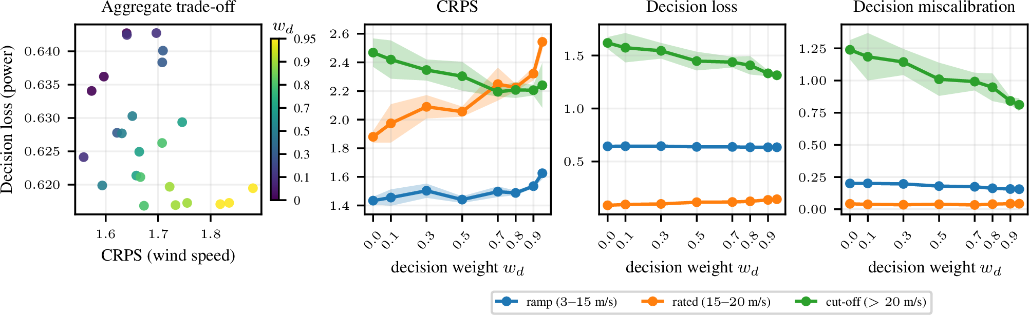
At the aggregate level (3, left), increasing \(w_d\) traces a consistent trade-off in the implicit generative model: decision loss improves while CRPS degrades, with \(w_d \approx 0.5\)–\(0.7\) offering the best balance. 3 disaggregates performance across all three power curve regions (for \(\lambda = 5\)). The effect of decision-aware training concentrates in the cut-off region (\(v > 20\) m/s 5), where forecast errors are most costly: at \(w_d = 0.9\), CRPS improves by 11%, decision cost by 18%, and decision calibration by 32% on average compared to \(w_d=0\). This improvement in the cut-off region comes at the cost of a slight degradation in CRPS and decision cost in the rated region (monotonically with \(w_d\)), and no effect in the ramp region. Consistent improvements are also observed for the diffusion model (10.2.3).
Cut-off improvements scale monotonically with \(\lambda\) in both models (12 17): higher penalty produces stronger corrections in the tail. However, at very high \(w_d\), CRPS degrades again, suggesting the decision loss overshoots the optimal distributional correction. The correction mechanism is further visible via a median shift \(\Delta Q_{0.5}(v)\) in the predictive distributions (13 18): corrections are negative in the ramp (more conservative dispatch) and positive beyond the cut-off threshold (more mass in the tail where power drops to zero). The decision calibration gap closes from both sides: observed cost decreases (trained objective) while the estimated expected cost increases, indicating more accurate cost estimation in both models; most visible in the cut-off region (14 19).
Mechanism. The regional pattern of improvements and degradations follows from how the decision-loss gradient propagates through the power curve. In the ramp region (\(\partial P/\partial y > 0\), \(a^*\) interior), gradients propagate and produce a shift to more conservative values in the predictive distribution, but aggregate metrics remain unaffected. In the rated region, \(\partial P/\partial y \approx 0\) suppressing the decision loss gradient, leaving CRPS at reduced weight \((1-w_d)\) and explaining the degradation. In the cut-off region, \(\partial P/\partial y \ll 0\) and \(a^*\) is interior; the gradient is strong, providing explicit supervision on the rare, high-cost tail events that CRPS under-weights due to their low frequency.
5.3 Frost Protection↩︎
Setup. Frost is among the most economically damaging meteorological hazards [24], [25], requiring decision makers to commit to protection resources before temperatures are observed. However, protection comes at a cost and should only be applied when required. We study this frost protection task in Berlin using ERA5 reanalysis data [23], forecasting temperature (at 2 m, T2m) 24 h ahead from lagged ERA5 temperature observations over a spatial patch, restricted to winter months. The decision maker chooses a frost protection level \(a \in [0, 1]\) before observing the realised temperature \(y\). The cost function has the same sigmoid threshold structure as in 5.1 (2, left), but mirrored: the hazard lies below rather than above the threshold. It penalises both unprotected frost (false negatives, FN) and unnecessary protection (false positives, FP), with \(\alpha\) controlling the FP/FN cost ratio such that lower \(\alpha\) penalises false negatives (unprotected frost) more heavily. Unlike the rare cut-off event in 5.2, frost occurs in approximately 25% of observations, making this a common event, where CRPS is less likely to under-weight the relevant area. We train an implicit generative model and a distributional diffusion model across \(w_d \in \{0.0, 0.1, \ldots, 0.9\}\) and \(\alpha \in \{0.2, 0.3, 0.5\}\) with three seeds (training details in 10.3.1); diffusion model results are in 10.3.3.
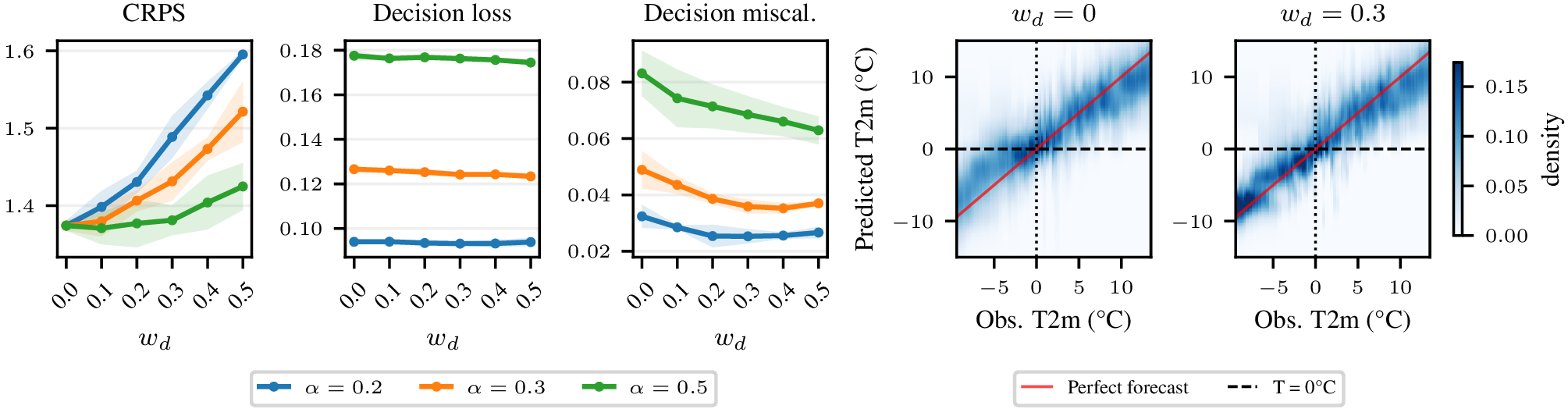
Results. At the aggregate level, CRPS degrades with \(w_d\), more steeply for lower \(\alpha\), while aggregate decision loss is mostly flat (4). For \(w_d > 0.5\), we observe spread collapse in many forecasts around the freezing point due to excessive decision loss correction. Decision miscalibration improves for all \(\alpha\), most visibly for \(\alpha=0.5\) by approximately 15% at \(w_d = 0.3\)–\(0.4\). Forecasts of sub-zero temperatures align more closely with observations when trained with decision loss (4, right). Unlike in wind power dispatch, where both decision cost and decision calibration improve, here decision calibration improves more visibly. We attribute this to the 25% base rate of frost: unlike the rare cut-off event, frost occurs frequently enough that CRPS already allocates substantial gradient signal to the threshold region, producing a near-optimal \(a^*\) even without the decision loss. The decision loss, therefore, has little room to shift \(a^*\) further, leaving aggregate cost unchanged. Decision calibration can nonetheless improve because even a near-optimal action leaves room to better estimate the expected cost \(\mathbb{E}[c(a^*, y)]\) from the model samples. A conditional breakdown (23) shows that the no-frost regime drives the improvement in decision calibration, while the frost regime degrades slightly.
Mechanism. Due to the sharp sigmoid cost function, the decision loss gradient is concentrated near the 0 °C threshold. Therefore, quantiles closer to the threshold (cost-sensitive region) shift more than those further away, as shown by the quantile shift plot in 24, aligning with the gradient analysis in 4.2. Unlike in the wind power cut-off region, many forecasts here straddle the threshold, making the decision loss gradient signal dense and its effects already visible at \(w_d = 0.1\)–\(0.2\), whereas wind power cut-off improvements require \(w_d \approx 0.5\)–\(0.7\) due to the rarity of cut-off events.
Together, the two real-world experiments show that our method adapts to the cost structure: in the wind power dispatch task, the gradient signal concentrates on rare high-cost tail events that CRPS underweights; in the frost protection task, it redistributes probability mass around a frequent threshold.
6 Related Work↩︎
The relevant prior work spans statistics, decision theory, and machine learning. These strands have not previously been connected; we combine them to enable decision-aware training of sample-based generative models.
Decision-focused learning. Decision-focused learning integrates the downstream decision task into the training objective, most commonly in predict-then-optimise pipelines where a point prediction is followed by a combinatorial or linear programme. [26] and [27] replace the prediction loss with a surrogate of the task loss. [5] embeds a differentiable optimisation layer and trains end-to-end. All target point predictions rather than distributions, and evaluate only task loss; we additionally measure decision calibration [6], which assesses whether the model correctly prices the cost of its own decisions. Our setting differs fundamentally: we work with probabilistic generative models that must produce forecast distributions, and the decision maker evaluates expected cost under the full distribution. To our knowledge, no existing decision-focused learning method operates in the sample-based generative model setting.
Weighted proper scoring rules. Weighted proper scoring rules [28], [29] emphasise specific regions of the outcome space, but require a fixed, pre-specified weight function. Additionally, they require a closed-form density or cumulative distribution function, making them incompatible with sample-based generative models. Our method requires no pre-specified weight: the decision loss gradient signal automatically concentrates on the cost-relevant region, which can change for different \(a^*\) and therefore adapts to the predicted distribution.
Differentiable optimisation. Differentiable optimisation layers [5], [18], [19] enable gradients to flow through the solution of an optimisation problem embedded in a neural network layer. We use this machinery to differentiate through the optimal action \(a^*\), connecting the decision loss to model parameters via implicit differentiation.
Generative weather models. State-of-the-art probabilistic ML weather prediction models increasingly use sample-based generative architectures, including diffusion-based [2], [30] and implicit generative [1], [31] approaches. We apply decision-aware training to representative architectures from these classes; the weather domain motivates this directly, as forecasts routinely inform high-stakes operational decisions where calibration in cost-relevant regions matters more than aggregate accuracy.
7 Conclusion↩︎
Decision-aware training for generative models is theoretically grounded and empirically effective, but its impact is selective. Whether a region of the output space receives a corrective signal depends on the optimal action: interior optima steer approximation errors toward less costly regions; boundary optima leave the original scoring-rule objective in full control. We demonstrated the mechanism on synthetic data, where decision-aware training corrects mode weight misattribution and improves downstream decisions; on wind power dispatch, where it concentrates improvements in the rare but costly cut-off region; and on frost protection, where it improves decision calibration.
A practical limitation is that the optimal decision weight \(w_d\) is task-dependent and requires tuning: at moderate \(w_d\), a sweet spot typically exists where decision loss improves with little degradation in distributional accuracy, but the right balance depends on the cost function and data regime. The method also requires a dedicated model per decision-maker, since the cost function is embedded into the training objective. The optimisation layer adds computational overhead at each training step; further details are provided in 9. For distributional diffusion models, our gradient analysis (4.2) characterises the decision loss training signal at the level of individual denoising steps, but does not account for inference-time reverse chain dynamics; a score-function formulation for the distributional denoiser could clarify when and why the effect carries through, and remains an open theoretical question.
Decision-aware training produces forecasts that are more actionable for specific downstream tasks, with direct applications in safety-critical domains such as weather hazard prediction, where better forecasts can directly reduce societal harm. A potential risk is that if the cost function encodes biased priorities, the model will optimise for them, potentially reinforcing skewed downstream decisions.
Extending decision-aware training to large-scale probabilistic weather prediction models [1], [31] is an interesting direction for future work. These systems share the same sample-based scoring rule training setup and are deployed in operational contexts where the gap between forecast skill and decision skill is operationally consequential.
8 Theory↩︎
This section provides a definition of the energy score, a proof of 1 and a detailed derivation of the decision loss gradient in 7 .
8.1 Energy Score↩︎
The energy score evaluates a predictive distribution \(\hat{F}\) against a realised outcome \(y\) via \[\mathrm{ES}(\hat{F}, y) = \mathbb{E}_{Y \sim \hat{F}}\|Y - y\| - \frac{1}{2}\mathbb{E}_{Y, Y' \sim \hat{F}}\|Y - Y'\|\] For sample-based models, both expectations are approximated by Monte Carlo estimates over \(M\) samples \(\{\hat{y}_m\}\) forming \(\hat{F}_M\): \[\mathrm{ES}(\hat{F}_M, y) = \frac{1}{M}\sum_{m=1}^M \|\hat{y}_m - y\| - \frac{1}{2M(M-1)}\sum_{m=1}^M\sum_{j=1}^M \|\hat{y}_m - \hat{y}_j\|. \label{eq:energy95score}\tag{8}\] For univariate targets the energy score reduces to the continuous ranked probability score (CRPS).
8.2 Proof of 1↩︎
Lemma 1. Let \(S_1\) be a strictly proper scoring rule and \(S_2\) be a proper scoring rule. Then \(S = (1-w_d)\,S_1 + w_d\,S_2\) is strictly proper for any \(w_d \in [0, 1)\).
Proof. The result follows immediately from the definitions. Let \(F\) be the true distribution and \(\hat{F} \neq F\) any forecast. Then \[\begin{align} \mathbb{E}_{Y \sim F}[S(\hat{F}, Y)] &= (1-w_d)\,\mathbb{E}[S_1(\hat{F}, Y)] + w_d\,\mathbb{E}[S_2(\hat{F}, Y)] \\ &> (1-w_d)\,\mathbb{E}[S_1(F, Y)] + w_d\,\mathbb{E}[S_2(F, Y)] \\ &= \mathbb{E}_{Y \sim F}[S(F, Y)], \end{align}\] where the strict inequality uses \(\mathbb{E}[S_1(\hat{F}, Y)] > \mathbb{E}[S_1(F, Y)]\) (strict properness of \(S_1\)) with weight \((1-w_d) > 0\), and \(\mathbb{E}[S_2(\hat{F}, Y)] \geq \mathbb{E}[S_2(F, Y)]\) (properness of \(S_2\)) with weight \(w_d \geq 0\). ◻
8.3 Finite-Sample Analysis of the Training Objective↩︎
8.4 Derivation of per-sample gradient (7 )↩︎
8.4.0.1 Problem setup.
Define \(f(a; \{\hat{y}_j\}_{j=1}^M) := \frac{1}{M}\sum_{j=1}^M c(a, \hat{y}_j)\); we write \(f(a)\) for brevity, making the sample dependence explicit only where the argument requires it. The optimal action solves \[\min_a\;f(a) \quad \text{s.t.} \quad a \geq a_\mathrm{min}, \quad a \leq a_\mathrm{max}. \label{eq:opt95problem}\tag{9}\] Since the feasible action set \([a_{\min}, a_{\max}]\) satisfies Slater’s condition, the KKT conditions are necessary at the optimal action \(a^*\). Rewriting the constraints in standard form \(g_1(a) = a_\mathrm{min} - a \leq 0\), \(g_2(a) = a - a_\mathrm{max} \leq 0\), the Lagrangian is \[\mathcal{L}(a, \mu_1, \mu_2) = f(a) + \mu_1(a_\mathrm{min} - a) + \mu_2(a - a_\mathrm{max}),\] with KKT conditions at \(a^*\): \[\begin{align} &\text{(stationarity)} & f'(a^*) - \mu_1 + \mu_2 &= 0, \label{eq:kkt95stat}\\ &\text{(dual feasibility)} & \mu_1,\, \mu_2 &\geq 0,\\ &\text{(complementary slackness)}& \mu_1(a^* - a_\mathrm{min}) &= 0, \quad \mu_2(a_\mathrm{max} - a^*) = 0, \end{align}\tag{10}\] where \(f'(a^*) := \partial f / \partial a\,(a^*)\).
8.4.0.2 Interior solution.
When \(a^*\) is interior, both constraints are inactive, so complementary slackness forces \(\mu_1 = \mu_2 = 0\) and all KKT conditions reduce to the first-order condition: \[f'(a^*) = \frac{1}{M}\sum_{j=1}^M \frac{\partial c}{\partial a}(a^*, \hat{y}_j) = 0. \label{eq:foc}\tag{11}\] To obtain \(\partial a^*/\partial \hat{y}_m\) we differentiate the optimality condition 11 implicitly with respect to \(\hat{y}_m\).
Implicit function theorem [19], [32] (IFT).
If \(F\colon \mathbb{R} \times \mathbb{R}^n \to \mathbb{R}\) is continuously differentiable with \(F(x_0, \theta_0) = 0\) and \(\partial F/\partial x \neq 0\) at \((x_0, \theta_0)\), then there exists a unique smooth function \(x^*(\theta)\) near \(\theta_0\) satisfying \(x^*(\theta_0) = x_0\) and \(F(x^*(\theta), \theta) = 0\).
Applying this with \(x = a\), \(\theta = \{\hat{y}_j\}_{j=1}^M\), and \(F(a; \{\hat{y}_j\}_{j=1}^M) := f'(a; \{\hat{y}_j\}_{j=1}^M)\), the IFT requires \(\partial F/\partial a \neq 0\) at \(a^*\): \[\frac{\partial F}{\partial a}\bigg|_{a^*} = \frac{1}{M}\sum_{j=1}^M \frac{\partial^2 c}{\partial a^2}(a^*, \hat{y}_j) =: H > 0,\] where \(H > 0\) follows from strict convexity of \(f\) at \(a^*\); the IFT therefore guarantees that \(a^*\) is locally a smooth function of \(\{\hat{y}_j\}_{j=1}^M\). In our setting, \(a^*\) is already defined as a function of \(\{\hat{y}_j\}\); the role of the IFT is therefore to establish smoothness of this function, licensing the implicit differentiation below — not to establish the functional dependence itself. Since \(F(a^*(\{\hat{y}_j\}); \{\hat{y}_j\}_{j=1}^M) = 0\) holds for all \(\{\hat{y}_j\}\), its total derivative with respect to any \(\hat{y}_m\) is zero; applying the chain rule gives \[\left.\frac{\partial F}{\partial a}\right|_{a^*} \cdot \frac{\partial a^*}{\partial \hat{y}_m} + \left.\frac{\partial F}{\partial \hat{y}_m}\right|_{a^*} = 0, \qquad \left.\frac{\partial F}{\partial \hat{y}_m}\right|_{a^*} = \frac{1}{M}\frac{\partial^2 c}{\partial a\,\partial \hat{y}_m}(a^*, \hat{y}_m),\] where only the \(j = m\) term in the sum contributes to \(\partial F / \partial \hat{y}_m\). Solving for \(\partial a^*/\partial \hat{y}_m\) gives Equation 7 in 4.2.
8.4.0.3 Boundary solution.
Consider \(a^* = a_\mathrm{max}\) (the case \(a^* = a_\mathrm{min}\) is symmetric). Since \(g_1\) is inactive, complementary slackness gives \(\mu_1 = 0\), and 10 becomes \[f'(a_\mathrm{max}; \{\hat{y}_j\}_{j=1}^M) = -\mu_2 \leq 0, \label{eq:boundary95grad}\tag{12}\] where the inequality follows from dual feasibility \(\mu_2 \geq 0\). Excluding the measure-zero case \(f'(a_\mathrm{max}) = 0\) (the unconstrained minimiser coincides exactly with \(a_\mathrm{max}\)), we have \(f'(a_\mathrm{max}) < 0\) strictly.
Since \(f\) depends on \(\hat{y}_m\) through the \(m\)-th summand, \(f'(a_\mathrm{max}; \{\hat{y}_j\}_{j=1}^M)\) is continuous in \(\hat{y}_m\) and therefore remains strictly negative under small perturbations \(\hat{y}_m \to \hat{y}_m + \delta\). Since \(f'(a_\mathrm{max})\) remains strictly negative (the objective still pushes beyond the boundary), the constraint \(g_2\) stays active and \(a^*\) stays at \(a_\mathrm{max}\); the multiplier \(\mu_2\) adjusts to maintain 10 without \(a^*\) moving. Consequently, \[\frac{\partial a^*}{\partial \hat{y}_m} = 0.\]
9 Implementation Details↩︎
Parts of our implementation build on code from [13], released under the MIT licence. Code for reproducing our experiments can be found at https://anonymous.4open.science/r/decision-aware-training-2114.
9.0.0.1 Training.
We use the Adam optimizer[33] with learning rate \(10^{-3}\) to train the models over \(2000\) epochs. Loss scales of CRPS and decision loss are estimated once before training and fixed throughout; optionally, a short CRPS pre-training phase precedes scale estimation to ensure realistic samples and cost values. We perform 200 epochs of CRPS pre-training for the wind power dispatch task, since we observe that untrained predictions yield outliers with non-realistic costs. We validate performance every 10 epochs on a validation set and apply early stopping with a patience of 600 epochs.
9.0.0.2 Distributional diffusion model.
The denoiser is an MLP with DDPM-style linear noise schedule over \(T=100\) steps, with 5 hidden layers of dimension 50 and ReLU activations. \(T=100\) is selected based on [12], [13], where improvements saturate for larger \(T\). We also ran pilot experiments with larger \(T\) but found no improvements. At each step the denoiser predicts a distribution over \(\epsilon\) (equivalently \(y_0\)) given noisy \(y_t\), drawing \(M\) samples per step. Conditional input \(x\) and a per-sample noise vector are injected via FiLM (Feature-wise Linear Modulation) conditioning at every hidden layer, giving each of the \(M\) samples a unique modulation.
9.0.0.3 Implicit generative model.
The implicit generative model is an MLP with 5 hidden layers of dimension 50 and ReLU activations. It maps the concatenation of conditioning input \(x\) and noise vector \(\varepsilon \sim \mathcal{N}(0, I)\) directly to a sample \(\hat{y}_m\); \(M\) independent noise draws in parallel yield \(M\) samples in a single forward pass.
9.0.0.4 Optimization layer.
The optimal action \(a^*\) is obtained via projected gradient descent on \(\frac{1}{M}\sum_m c(a, \hat{y}_m)\) over \(\mathcal{A}\), implemented within
the optimization layer forward pass. We use 50 optimization steps during training, which small pilot experiments confirmed to be sufficient for convergence; at inference we use 200 steps for higher precision. Second-order derivatives required for computing
the decision loss gradient (7 ) are computed via PyTorch autograd.
Decision-aware training adds computational overhead relative to standard energy score training through the optimisation layer, which is invoked at every forward pass. The overhead scales with the number of samples \(M\) (the optimisation objective is evaluated over all \(M\) samples per batch element) and the number of iterations required to solve 1 to convergence.
9.0.0.5 Computational resources
We use an internal compute cluster with NVIDIA A100 GPUs. Training of all models required approximately 50 GPU hours.
9.0.0.6 Data
The ERA5 dataset used in the real-world experiments s provided by the Copernicus Climate Change Service under a licence permitting research use [23].
10 Additional Results↩︎
This section presents additional experimental details and results for all three experiments in the main paper.
10.1 Synthetic Decision Task↩︎
We use a 1600/200/400 train/val/test split across 3 data seeds and 3 training seeds, training a distributional diffusion model. The denoiser uses \(M=10\) samples during training. At inference, we draw 200 samples from the learned predictive distributions via independent reverse chain runs. The cost function belongs to the same sigmoid threshold family as the frost hazard cost; strict convexity of the expected cost at interior solutions is verified in 10.3.1.
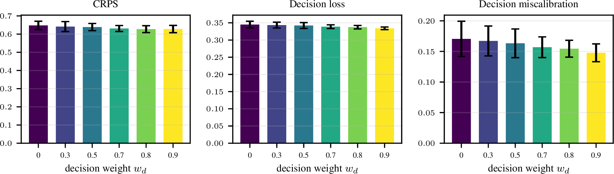
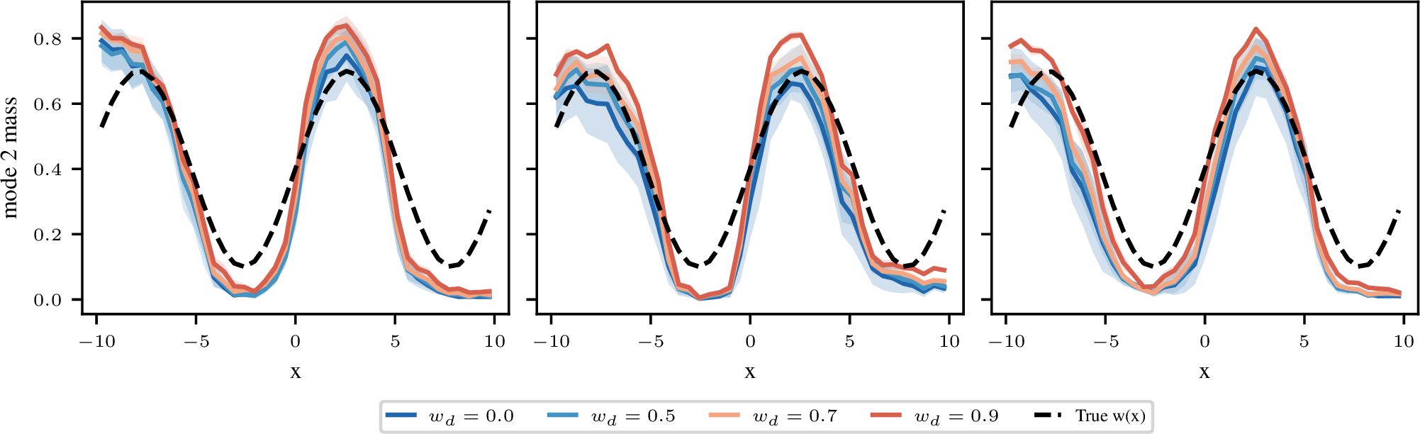
5 shows the data generating process (bimodal conditional GMM with input-dependent mode weights and ground-truth optimal action \(a^*(x)\)). 6 shows aggregate CRPS, decision loss, and decision calibration vs.\(w_d\), pooled across all seeds. 7 shows the predictive marginal distributions across seeds and \(w_d\) values: mode 1 is heavily overrepresented at \(w_d=0\) (CRPS failure), with mode 2 mass progressively recovering as \(w_d\) increases. 8 shows the predicted \(a^*(x)\) across data seeds and \(w_d\): tracking improves consistently, though some of the troughs (boundary \(a^*=0\), no gradient) remain a blind spot. 9 shows the conditional mode 2 mass as a function of input \(x\): dec loss partially recovers the true \(w(x)\) around the peaks but overshoots at high \(w_d\).
10.2 Wind Power Dispatch↩︎
In this section we report experimental details of the wind power dispatch experiment followed by additional results for the implicit generative model as well as results for the distributional diffusion model on this task.
10.2.1 Experimental setup↩︎
The power curve maps 10m wind speed to normalised power output via a differentiable sigmoid approximation [34]; hub-height wind speeds are recovered via a power-law profile [35]. The dispatch cost is \(c(a,y) = -a + \lambda\,\mathrm{relu}(a - P(y))^2\), where \(a \in [0,1]\) is the committed power fraction, \(P(y)\) is the normalised power output, and \(\lambda\) controls the shortfall penalty. We do not apply a penalty for power overproduction since this case can be avoided by windpower providers by dynamically reducing power output (curtailment) to match the promised amount [20]. In this case, only opportunity costs remain (\(c=-a\)), since a larger \(a\) could have been chosen to increase revenue.
ERA5 inputs are observed wind speed at \(t\), \(t{-}6\) h, and \(t{-}12\) h. We use 2005–2019 for training, 2020 for validation, and 2021 for testing. The test set contains 105 cut-off events (\(v > 20\) m/s at hub height), 230 rated, and 1074 ramp observations. The implicit generative model uses \(M=10\) samples during training and \(M=500\) at inference. The distributional diffusion model uses \(M=10\) samples for the probabilistic denoiser during training; at inference, 500 samples are drawn via independent reverse chain runs.
Strict convexity of \(f(a) = \frac{1}{M}\sum_j c(a,\hat{y}_j)\) (8.4) at interior solutions holds analytically: since \(\frac{\partial^2}{\partial a^2} c(a, \hat{y}_j) = 2\lambda\) when \(\hat{y}_j < a\) and \(0\) otherwise, we have \(H = (2\lambda/M)\,\#\{j : P(\hat{y}_j) < a^*\}\). At any interior \(a^*\), at least one sample must satisfy \(\hat{y}_j < a^*\) — otherwise \(f'(a^*) = -1 < 0\), contradicting optimality — so \(H > 0\).
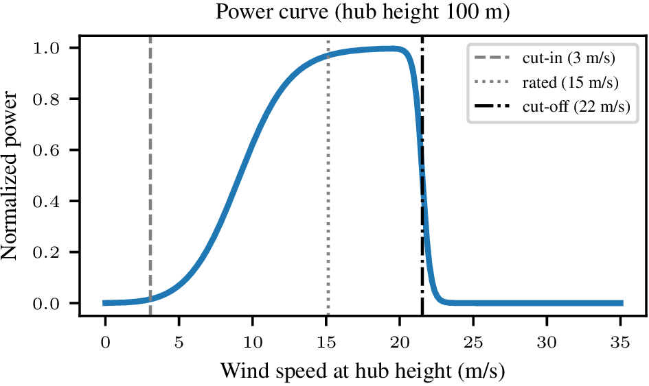
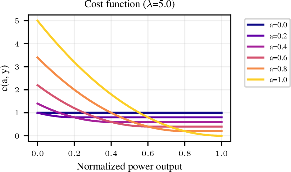
Figure 10: Left: differentiable power curve used for converting wind speed at turbine hub height to normalized power output. Right: dispatch cost \(c(a,y)\) for \(\lambda = 5\) as a function of committed power \(a\) and observed power output \(y\)..
10.2.2 Additional results: implicit generative model↩︎
11 shows the aggregate CRPS vs decision loss trade-off across seeds and \(w_d\) and the regional breakdown for \(\lambda=3\) and \(\lambda=10\) (the main text shows \(\lambda=5\)). 12 shows the cut-off region ablation across \(\lambda\): improvements scale monotonically with \(\lambda\). 13 shows the rolling-window median shift \(\Delta Q_{0.5}(v)\): the correction is negative in the ramp region, reverses beyond cut-off, and its magnitude (in ramp region) tracks the power curve slope. 14 shows the decision calibration decomposition for \(\lambda \in \{3, 10\}\).


Figure 11: Same plot as 3 in main text (\(\lambda = 5\)), for \(\lambda = 3\) (top row) and \(\lambda = 10\) (bottom row); implicit generative model. Left column: Aggregate CRPS vs decision loss trade-off across seeds and \(w_d\) for \(\lambda \in \{3, 10\}\). Right (three columns): Regional metrics (cut-off, ramp, rated) vs \(w_d\) for \(\lambda=3\) (top) and \(\lambda=10\) (bottom). Cut-off improvements are strongest for \(\lambda=10\), confirming that higher shortfall penalty amplifies the gradient signal in the cut-off region..


![Figure 14: Decision calibration decomposition for \lambda=3 (left) and \lambda=10 (right), implicit generative model. Each bar shows the test-set average of one side of 3 : average observed cost \frac{1}{N}\sum_n c(a^*_n, y_n) and average estimated expected cost \frac{1}{N}\sum_n \mathbb{E}_{\hat{y}}[c(a^*_n, \hat{y})]. The observed cost decreases (training objective) while the estimated expected cost increases, indicating more accurate cost estimation; both bars move toward each other with increasing w_d. Note that the experiment results in the main text (decision miscalibration) use a stronger variant to compute this gap by averaging per-sample absolute differences. The gap between bars in this plot, therefore, provides a lower bound on decision miscalibration reported in the main paper.](/article/2607.01171/figures/final/appendix/windpower/mlp_regression/mlp_regression_sharp5_cal_decomp_icml.png "fig:")
10.2.3 Distributional diffusion model results↩︎
15 shows aggregate metrics vs \(w_d\): CRPS improves then overshoots at high \(w_d\); aggregate decision loss is flat; decision calibration improves consistently for all \(\lambda\). 16 shows the full regional breakdown for each \(\lambda\). 17 shows the cut-off region ablation across \(\lambda\). 18 shows the rolling-window median shift. 19 shows the decision calibration decomposition for \(\lambda \in \{3, 10\}\).


![Figure 19: Decision calibration decomposition for \lambda=3 (left) and \lambda=10 (right), distributional diffusion model. Each bar shows the test-set average of one side of 3 : average observed cost \frac{1}{N}\sum_n c(a^*_n, y_n) and average estimated expected cost \frac{1}{N}\sum_n \mathbb{E}_{\hat{y}}[c(a^*_n, \hat{y})]. The observed cost decreases (trained objective) while the estimated expected cost increases, indicating more accurate cost estimation; both bars move toward each other with increasing w_d. Note that the experiment results in the main text (decision miscalibration) use a stronger variant to compute this gap by averaging per-sample absolute differences. The gap between bars in this plot, therefore, provides a lower bound on decision miscalibration reported in the main paper.](/article/2607.01171/figures/final/appendix/windpower/mlp_diffusion/mlp_diffusion_sharp5_cal_decomp_icml.png "fig:")
10.3 Frost Protection↩︎
In this section we report experimental details of the frost protection experiment followed by additional results for the implicit generative model as well as results for the distributional diffusion model on this task.
10.3.1 Experimental setup↩︎
ERA5 inputs are 2 m temperature from a \(3{\times}3\) spatial patch (centered around the target grid point) at three time steps (27 features), restricted to November–March. The implicit generative model uses \(M=10\) samples during training and \(M=500\) at inference. The distributional diffusion model uses \(M=10\) samples from the probabilistic denoiser during training; at inference, 500 samples are drawn via independent reverse chain runs. The cost function is a sigmoid threshold at \(0\) °C; \(\alpha = \frac{FP}{FN}\) controls the asymmetry between false positive and false negative costs (20). The gradient derivation requires strict convexity of \(f(a) = \frac{1}{M}\sum_j c(a, \hat{y}_j)\) (8.4) at interior solutions; this was verified empirically across 100,000 randomly drawn sample sets of size \(M=50\) from the marginal training distribution, with \(H > 0\) (strict convexity) in all cases.

10.3.2 Additional results: implicit generative model↩︎
The main text shows aggregate metrics for all \(\alpha\) values and the conditional KDE for \(\alpha=0.3\). 21 shows the conditional KDE for all three \(\alpha\) values at \(w_d=0.3\), alongside the shared \(w_d=0\) baseline. 22 shows the marginal 2m temperature (T2m) distributions for \(\alpha=0.5\): a cold mode missed by pure CRPS (\(w_d=0.0\)) progressively aligns with the observed distribution at the sweet spot \(w_d=0.3-0.5\), before shifting slightly beyond it at \(w_d=0.9\). 23 shows the conditional breakdown by frost and no-frost observations for \(\alpha \in \{0.2,0.3,0.5\}\), the no-frost regime improves in terms of decision calibration while the frost regime degrades slightly or stays constant across \(w_d\). 24 shows the quantile shift in the predictive distributions introduced through decision loss training: quantiles closer to the cost-sensitive threshold region get shifted more strongly, supporting the claim of probability mass being redistributed around the decision threshold.


10.3.3 Distributional diffusion model results↩︎
For the distributional diffusion model, the decision loss does not improve the forecast distributions as expected. The baseline (\(w_d=0\)) already exhibits a cold bias: for sub-zero observations, the conditional forecast distribution is shifted toward colder temperatures relative to the observed values, as visible in the KDE plots (25). Decision loss training (\(w_d > 0\)) does not correct this artifact. CRPS degrades monotonically for larger \(w_d\) in all \(\alpha\) settings, yet, decision miscalibration improves for \(\alpha < 0.5\). Notably, the same sigmoid cost function with a distributional diffusion model yields clear improvements on the synthetic decision task (5), so the failure is not inherent to the cost structure or model class. We do not have a complete explanation for this failure mode, one hypothesis is that samples from the baseline model (\(w_d=0\)) are already outside of the strong gradient region of the cost function (too cold), thus the decision loss has no handle to correct them. We also note that the reverse chain dynamics at inference time are not captured by the per-step training objective (7), potentially introducing compounding errors at inference.

References↩︎
We use \(y_0, y_t\) for the clean and noisy target following our regression notation; the standard diffusion literature uses \(x_0, x_t\).↩︎
In fact, distribution calibration [15] would suffice for optimal decisions, but even this weaker condition is not attainable nor verifiable in practice, motivating a focus on decision calibration directly [16], [17]↩︎
The result is even stronger: the space of decision losses induced by arbitrary bounded cost functions is equivalent to the space of proper scoring rules [7], [8] — every proper scoring rule arises as the optimal action cost of some cost function.↩︎
The measure-zero case where the unconstrained minimiser coincides exactly with the boundary is excluded.↩︎
We use 20 m/s as the analysis threshold rather than the physical cut-off speed of 22 m/s to include events near the cut-off where power is already falling sharply.↩︎